Aggregation and the law of large numbers in large economies

b

chastictize’ thehas aargethings,in the

piricalhanism

ber ofture are

Games and Economic Behavior 47 (2004) 1–35www.elsevier.com/locate/ge

Aggregation and the law of large numbersin large economies

Nabil I. Al-Najjar

Department of Managerial Economics and Decision Sciences, Kellogg School of Management,Northwestern University, Evanston, IL 60208, USA

Received 26 August 2002

Abstract

This paper introduces a new model of environments with a large number of agents and stocharacteristics. We consider sequences of finite but increasingly large economies that ‘discrecontinuum. In the limit we obtain a model that is continuum-like in important respects, yet itcountable set of agents with a finitely additive, ‘uniform’ distribution. In this model, the law of lnumbers is meaningful and holds on all subintervals. This framework provides, among othera new interpretation of the measurability problem and the failure of the law of large numberscontinuum. It is also shown that the Pettis integral in the continuum coincides with the emfrequencies in the discrete model almost surely. Finally, the model is used to study a mecdesign problem in a large economy with private information. 2003 Elsevier Inc. All rights reserved.

JEL classification: C7; C6; H41

1. Introduction

This paper introduces a new approach to model environments with a large numagents and stochastic characteristics. The two standard approaches in the literabased on either

(1) a sequence of finite but increasingly large sets of agents, or(2) a continuum of agents.

E-mail address: [email protected].

0899-8256/$ – see front matter 2003 Elsevier Inc. All rights reserved.doi:10.1016/S0899-8256(03)00175-1

2 N.I. Al-Najjar / Games and Economic Behavior 47 (2004) 1–35

d with

helds, in

ys:ion off agentiscretecationseable

ndomementation’hisroof isriables.ouslyelated

rature.ies as aosedensityldmanBewleyinuum.detailed

ty torovidet witheffectandber ofiduallynomyxtendcy is6).

The paper proposes a ‘hybrid’ model that eliminates many of the problems associate(and provides a new interpretation of) these two common modeling approaches.

We consider a sequenceTN ∞N=1 of finite but increasingly large economies. Tsequence is chosen so it ‘discretizes’ the continuum in a natural sense and yiethe limit, a model with afinitely additive distribution on a countable set of agents.Although discrete, the limiting model we construct is ‘continuum-like’ in important wait preserves the interval and metric structures of the continuum, and the distributagents is ‘uniform’ and atomless. A rich class of independent stochastic processes ocharacteristics can be ‘translated’ back and forth between the continuum and our dmodel in an essentially unique manner. This class encompasses virtually all specifiused in applications, including all i.i.d., conditionally independent, and exchangdistributions.

The law of large numbers states that the empirical frequency of independent ravariables is almost surely equal to the population mean. It is well known that this statis problematic in the continuum because the ‘empirical frequency of a sample realizcannot be meaningfully defined.1 By contrast, in the discrete model introduced in tpaper, the law of large numbers has a straightforward formal statement and its pa natural extension of the usual proof for a sequence of independent random vaIt is also straightforward to show that the law of large numbers holds simultaneon all subintervals, and can be extended to non-identically distributed and/or corrdistributions.

Although new, the approach advocated here builds on two ideas already in the liteFirst, Bewley (1986) and Guesnerie (1981, 1995) proposed modeling large economsample of agentst1, . . . randomly drawn from the continuum. The second idea, propby Feldman and Gilles (1985), is to use an infinite sequence of agents with a dcharge.2 This paper combines the strengths of the above authors’ insights. Like Feand Gilles (1985), this paper uses density charges on a countable index set, and like(1986) and Guesnerie (1981), our model maintains a close connection to the contThe differences with these two approaches are substantial, however, and they arein Section 5.

The usefulness of a formal model of large economies is judged by its abiliaddress economic questions. In Section 6, I use the framework of this paper to pa large-economy formulation of a mechanism design problem in an environmenprivate information. Rob (1989) and Mailath and Postlewaite (1990) examined theof private information on efficiency in finite-agent economies with externalitiespublic goods. They showed that in a sequence of finite but increasingly large numagents and independent types, the outcome of any incentive compatible and indivrational mechanism is asymptotically inefficient. In Section 6, I provide a large-ecoformulation of this model and explain how the concepts of mechanism design theory eto such environments. In this limiting model, exact (rather than asymptotic) inefficieneasily established using the concept of influence in Al-Najjar and Smorodinsky (199

1 Judd (1985) and Feldman and Gilles (1985). See Section 4 for a detailed discussion.2 That is, a uniform, finitely additive distribution on the integers.

N.I. Al-Najjar / Games and Economic Behavior 47 (2004) 1–35 3

oints.ymous

result,ewedminateseserves

econd,anisms are

ithout a

k inlevel,

it hasovidesrem 6)iscretea way). The

enciesPettis

hemat-3). Al-for in-

ction 2,agentseworkhe ap-

modelblishesitiveof the

finitelyuires

doversists ofthatitely

asuresatsui

ount of

The mechanism design example of Section 6 illustrates a number of important pIn the setting of that example, it would be unreasonable to restrict attention to anonmechanisms (ones where two agents of the same type are treated identically). As aa distributional model of a large economy—i.e., where the large economy is vias a measure on a space of characteristic—may be inappropriate because it eliagents’ labels and thus forces mechanisms to be anonymous. Our framework pragents’ labels and thus has no problem handling non-anonymous mechanisms. Sthe example illustrates the need for a strong law of large numbers in studying mechdesign problems in large economies with private information. In the example, typeindependent, so many natural classes of mechanisms are not even well-defined wstrong law of large numbers (e.g., to compute aggregate transfers).

The well known technical problems associated with introducing idiosyncratic risthe continuum did not slow down its wide-spread use in applications. At an intuitivethe continuum does appear to ‘make sense’ as a model of large economies andindeed proved valuable in generating important economic insights. This paper prsome support for such practice. Specifically, I prove a simple characterization (Theostating that the Pettis integral in the continuum and the empirical frequencies in the dmodel coincide almost surely. The Pettis integral was suggested by Uhlig (1996) asto formulate a weak law of large numbers for the continuum (see Sections 3.5 and 5problem is that the Pettis integral has no obvious meaning in terms of empirical frequof sample realizations. The above mentioned result provides a way to interpret theintegral in a way suggestive of a strong law of large numbers for the continuum.

Finitely additive measures (and, in particular, density charges) are standard matical tools—see, for example, Dunford and Schwartz (1958) and Rao and Rao (198though used extensively in certain research fields (such as Decision Theory; see,stance, Fishburn, 1970), they are uncommon as models of large economies. In SeI discuss two problems that might have led to the limited use of countable models ofand a finitely additive measure, and explain how they can be remedied using the framintroduced here. The application to mechanism design in Section 6 further illustrate tplicability of our model to concrete economic settings.

Some of the earliest published work using finitely additive measure spaces tolarge economies are Weiss (1981), Armstrong and Richter (1984, 1986). Weiss estathe equivalence of core and competitive allocations in a model with a finitely addspace of agents. Armstrong and Richter (1984) provide a more general treatmentsame problem covering, among other things, countable spaces of agents withadditive measures. They point out that formulating coalitions in the continuum reqthe unconvincing assumption that the set of coalitions be aσ -algebra. Armstrong anRichter (1986) prove a general result on the existence of competitive equilibria that cthe environments of their earlier paper. The argument they use in the proof consmapping the finitely additive model into a countably additive one. They then showthe existence proof in the countably additive model carries back to the original finadditive environment they started with. Other subsequent uses of finitely additive mein Economics and Game Theory include Feldman and Gilles (1985), Gilboa and M(1992), Werner (1997), Marinacci (1997). See these papers for more exhaustive accthe literature.


e one

95).

recentbased

internaler-reald hereks and

gents,

ite

ssion

nd

Three approaches to modeling large economies are directly comparable to thpresented in this paper. These are:

(1) the sampling approach of Bewley (1986) and Guesnerie (1981, 1995);(2) density charges on a countable set of agents (Feldman and Gilles, 1985); and(3) linear methods relying on variants of the Pettis integral (Uhlig, 1996; Al-Najjar, 19

I provide a detailed comparison with these approaches in Section 5. A moreinteresting approach is that introduced by Sun (1998) and Khan and Sun (1999)on hyperfinite Loeb spaces. In these papers, the space of agents is a hyperfiniteprobability space that includes non-standard entities (e.g., infinitesimals and hypnumbers). This approach appears to be sufficiently different from the one introducethat a detailed comparison is difficult. The interested reader may refer to these worto the references therein for further details.

2. Three models of large economies

2.1. The continuum and its discretization

Our starting point is the standard model of a large economy as a continuum of aT = [0,1], with the uniform distributionλ.3

We would like to think of the continuumT as an idealization of a sequence of finmodels,TN ∞N=1, where theN th model has the form

TN = t1, . . . , t#TN ⊂ T , N = 1,2, . . . .

The uniform distribution onTN , denotedλN , assigns to each subsetA ⊂ TN a measureequal to its relative frequency:

λN(A)≡ #A

#TN.

Notational conventions. It is convenient to think ofλN as a distribution onT with supportTN so λN and λ are defined on the same space. With this convention, the expreλN([a, b]) has an unambiguous meaning asλN (TN ∩ [a, b]). We may thus useλN andTN interchangeably to talk about theN th model, sinceTN is just the support ofλN .

We assume that the sequenceTN ∞N=1 asymptotically has the same interval ameasure structures as the continuumT :

Definition 1. A discretizing sequence TN ∞N=1 is one satisfying:

(1) TN ⊂ TN+1 for everyN ; and(2) The sequence of finite distributionsλN converges weakly toλ.

3 The continuum [0,1] is endowed with theσ -algebraT of the Borel sets.


e

plies

lders toite,

kingulties

led

neverof

n

that the

ls

can be

m

Using a standard characterization of weak convergence,4 condition 2 is equivalent to threquirement: for every non-degenerate interval of agents[a, b] ⊂ [0,1],5

limN→∞λN

([a, b])= λ([a, b]). (1)

That is, the mass of agents inTN who fall within a given interval[a, b] asymptoticallycoincides with the corresponding mass of agents in the continuum. Note that this imthat

⋃∞N=1TN must be dense inT .6

2.2. The large discrete model

Fix a discretizing sequenceTN ∞N=1. Intuitively, asN becomes large, one wouexpect individual agents to have vanishing weight and for the law of large numbapproximately hold asN goes to infinity. In the limit, when the number of agents is infinone would expect these properties to holdexactly.

What is the ‘right limit’ for a sequence of increasingly large, finite economies? Tathe continuumT to be that limit, each agent indeed has zero weight, but serious difficarise in stating the law of large numbers. Here I introduce a new model,T , as a limit of thesequenceTN ∞N=1. The setT satisfiesTN ⊂ T ⊂ T and has the special structure detaibelow:7

Theorem 1. Fix any discretizing sequence TN ∞N=1 and define T =⋃∞N=1 TN . Then there

is a finitely additive probability measure λ on 2T such that

λ(A)= limN→∞λN (A) (2)

for every A⊂ T for which the limit exists.

A measureλ with the properties asserted in Theorem 1 is known as adensity chargeonT . Such measure assigns to every set its limiting frequency (the RHS of (2)) whethis frequency is well defined. The theorem says thatλ can be extended to every subsetagents in an additive fashion.

Definition 2. A discretization of T is a pair (TN ∞N=1, λ) satisfying the properties iTheorem 1.8

4 See, for instance, Shiryayev (1984, Theorem 1, p. 309). To apply that theorem, it suffices to noteboundary of the interval[a,b] hasλ-measure 0.

5 Throughout the paper, an ‘interval’ will refer to a set[a,b] with a < b. This rules out degenerate intervaof the form[a,a].

6 Constructing a discretizing sequence is straightforward. For instance, one can chooseTN by induction asTN+1 = k/(N + 1)N+1

k=0 ∪ TN .7 All proofs are in Appendix A. Except for a minor change, Theorem 1 is just the standard result that

found, say, in Rao and Rao (1983, p. 41) or Feldman and Gilles (1985).8 When TN and/orλ is clear from the context, we may refer to(T ,λ) or just T as a discretization. Any

sequenceTN ∞N=1 gives rise to a uniqueT ; conversely, a givenT has meaning in this paper only if it arises fro

a sequence of finite modelsTN satisfying Eq. (2).


yn thecy.

nts,ons to

ows

. Note

0) showticular

roduce

This construction has several implications: First, any such measure must beatomless9

so, as with the continuum,λ assigns zero mass to any individual agent. Second,λ cannot becountably additive sinceT is countable,λ(t) = 0 for everyt ∈ T , butλ(T )= 1.10 Third,the value ofλ is completely pinned down for setsA ⊂ T whose asymptotic frequencis unambiguously defined and these include, by Eq. (1), the set of all intervals. Oother hand,λ is not uniquely defined for sets without a well-defined limiting frequenLater we introduce additional structure that makes the indeterminacy ofλ irrelevant (seeTheorem 2).

2.3. Integration

Functions of the formf :T → R will be used to represent agents’ endowmetransfers, types, etc. We are interested in integrating (averaging out) such functiobtain average endowment, transfers and so on. The integral

∫T f dλ with respect to a

density chargeλ is well defined and extensively studied; its development closely follthat of the usual integral.11 For a simple function f , i.e., a function with finite rangex1, . . . , xK, define

∫T

f dλ≡K∑k=1

xkλ(t : f (t)= xk

). (3)

That is, the integral is just the average of its values weighted by their frequenciesthat this is well defined forany simple function, since every subset ofT is measurable.

For more general functions, we have:

Definition 3. The integral of a bounded functionf :T → R is∫T

f dλ= limn→∞

∫T

fn(t)dλ,

wherefn :T → R, n ∈ N, is any sequence of simple functions such thatfn converges tofuniformly.

Standard results (e.g., Rao and Rao, 1983, Chapter 4, or Fishburn, 1970, Chapter 1that this integral is well defined for all bounded functions, does not depend on the parapproximating sequencefn, and satisfies the basic properties of integrals.

9 The limiting frequency of any finite sett1, . . . , tm is zero, henceλ assigns weight zero to such sets.10 In fact,λ is purely finitely additive: Ifη is anycountably additive measure on(T ,2T ) such thatη(A) λ(A)

for everyA⊂ T , thenη(A)= 0 for everyA⊂ T . See Rao and Rao (1983, p. 240). The fact thatλ is purely finitelyadditive follows from Theorem 10.3.2 in Rao and Rao.

11 Dunford and Schwartz (1958) develop the theory integration for finitely additive measures, then intcountable additivity as a special case. Rao and Rao (1983) is a more specialized reference.


e

toesprice.

an beeorem

larges,with

it (see

n

eful tothat

It is convenient to define integration with respect toλN , which reduces to taking thsimple average of a function overTN :12∫

T

f dλN ≡ 1

#TN

∑t∈TN

f (t).

Notational convention. Using our convention to viewλN as a measure onT withsupportTN , givenf :A→ R it is legitimate to write:∫

TN

f dλN =∫B

f dλN, wheneverTN ⊂A⊂ B ⊂ T .

For example,∫ baf dλN is meaningful forf :T → R (hereB = [a, b] andA= T ∩B).

2.4. Functions with well-behaved frequencies

From Section 2.3 we know thatany bounded function is integrable with respectthe finitely additive probabilityλ. Despite this, models with finitely additive probabilitiattracted little interest in the literature because the freedom they offer comes at aProblems include that finitely additive probabilities allow ‘mass to disappear’; they chard to interpret as limits of large finite models; and basic results such as Fubini’s thmight fail.

In Section 6, I illustrate these problems in the context of mechanism design ineconomies. Here, I simply introduce a class of extremely well-behaved functionF ,and show that they do not suffer from many of the problems common in modelsfinitely additive probabilities. Another, independent reason for consideringF is thatevery typical realization of an independent stochastic process must belong toTheorem 4).

2.4.1. Functions with well-defined distributionsFor a function on the continuumf :T → R, andr ∈ R, we have the standard definitio

of a cumulative distribution function (cdf):

F(r, [a, b])≡ 1

|a − b| λ(t ∈ [a, b]: f (t) r

),

which must be non-decreasing and right-continuous inr. These properties of cdf’s aressential in applications and follow as a by-product of countable additivity. It is usenote that right-continuity in the continuum follows from a more basic property, namelyfor everyr ∈ R and interval[a, b]:

λ(t ∈ [a, b]: f (t)= r

)= infr ′>r

F(r ′, [a, b])− sup

r ′<rF(r ′, [a, b]). (∗)

12 The integralf on a subsetA is covered by this notation, since∫A f dλ ≡ ∫

T χAf dλ, whereχA is theindicator function ofA.


d that

der

. In they.

do

Things are quite different in the discrete model where it is no longer guaranteemass behaves continuously under limits. Let

F(r, [a, b])≡ 1

|a − b|λ(t ∈ [a, b]: f (t) r

).

Definition 4. A function f :T → R haswell-behaved distribution function if for everyinterval[a, b] andr ∈ R,

λ(t ∈ [a, b]: f (t)= r

)= infr ′>r

F(r ′, [a, b])− sup

r ′<rF(r ′, [a, b]). (4)

Without this restriction,F(·, [a, b]) may fail to be right-continuous. To see this, consithe following example:

Example 1. Definef :T → R by:f (t)= 1 for t ∈ T1, andf (t)= 1/N for t ∈ TN −TN−1,N > 2. Then for everyr > 0, λf (t) r = 1, yet λf (t) 0 = 0. In particular,∫T f dλ= 0.13

In this example,F(r, [0,1]) = 1 for every r > 0, but 1= limr↓0F(r, [0,1]) =F(0, [0,1])= 0, soF is not a distribution function. The problem is that points at whichfis less thanr has mass 1 for everyr > 0, but this mass disappears in the limit whenr = 0.

Mass may also escape “from below,” as seen by examining the function−f , whichhas a well defined distribution function, but mass disappears, this timeupward to zero.In both cases, mass accumulates at a point, but the mass of the point itself is zerocontinuum, discontinuity at the limit isindirectly ruled out through countable additivitWith finitely additive probabilities, this discontinuity must be ruled out explicitly, as wein Definition 4.

2.4.2. Functions with asymptotic frequenciesAnother issue is the relationship between the limiting modelT and large finite

models,TN . Define the cdf relative toTN as

FN(r, [a, b])≡ 1

|a − b|λN(t ∈ [a, b]: f (t) r

).

The following example shows thatFN andF need not be related.

Example 2. Fix 0< ε < 12 and an increasing sequence of integersNk such thatNk+1 >

Nk/ε. Fork 2, letf (t)= 0 if t ∈ TNk+1 − TNk for oddk andf (t)= 1 for evenk. Then

lim infN→∞

∫T

f (t)dλN < ε < 1− ε < lim supN→∞

∫T

f (t)dλN .

13 To prove these claims,λf (t) 0 = 0 is obvious sincef is strictly positive;λf (t) r = 1 follows fromthe facts thatf (t) < r for t ∈ T − TN for N large enough so the setf (t) > r is finite and hence hasλ-measurezero. Finally,

∫T f dλ= 0 follows from similar reasoning.


c

nd

Although the integral∫T f (t)dλ in this example is a well-defined number in[0,1], it bears

no connection to the integrals in large finite models,∫Tf (t)dλN , which fluctuate wildly

asN changes. In the example, the problem is that the limitf reflects poorly the asymptotibehavior of the distributions in finite models.

To address the issue raised by this example, we introduce the restriction:

Definition 5. A functionf :T → R hasasymptotic frequencies if for every interval[a, b],

FN(·, [a, b])→ F

(·, [a, b]) weakly.

Note that limN→∞ λN (A) exists if and only if the indicator functionχA :T → R hasasymptotic frequencies on[0,1].

2.5. Integration revisited

We combine the last two definitions to obtain

Definition 6. F is the set of all functions with well-defined distribution functions aasymptotic frequencies.

2.5.1. Integration of functions in F is extremely well behavedTheorem 2. For any f ∈F and interval [a, b],

(1) F(·, [a, b]) is a distribution function.(2) Change of variables:

1

|a − b|b∫a

f dλ=∫R

r dF(r, [a, b]). (5)

(3) The integral in the limit is the limit of integrals in finite models:

b∫a

f dλ= limN→∞

b∫a

f dλN. (6)

In particular, the integral∫ ba f dλ of a function f ∈ F does not depend on the particular

extension λ chosen in Theorem 1.


e

s allyn as at

pe,f

hee case

in

n

2.5.2. Piecewise uniformly continuous functionsAn important class of functions we shall use is

Definition 7. The set ofpiecewise uniformly continuous functions, denotedC, is the setof all functionsf :T → R such that for some real numbers 0= a1 < · · ·< aM = 1, f isuniformly continuous on every ‘interval’(am−1, am)∩ T .14

We defineC similarly for functionsf :T → R.15

In Section 4.2 we show that there exists betweenC andC a natural (essentially) one-onand onto mapping that preserves integration. For the moment we simply note:

Theorem 3. C ⊂F .

In summary,F is a rich and extremely well-behaved class of functions: It includepiecewise uniformly continuous functions; the integral of anyf ∈ F can be computed bintegrating the corresponding cdf; and any such function has a natural interpretatiolimit of a sequence of functions in the finite models. Our interest inF stems from the facthat a typical realization of an independent random process must belong toF (Theorem 4),yet such realizations cannot even be approximated by functions inC (Section 4).

3. The law of large numbers

We will consider models where each agentt has a random characteristic (e.g., his tyendowment, and so on), modeled as a random variables(t) taking values in some set ocharacteristicsS.

We first consider the special caseS = 0,1 to illustrate the paper’s main ideas in tsimplest possible setting. In Section 3.8, we show how to extend the analysis to thwhereS is an arbitrary finite set.

3.1. The law of large numbers in the discrete model

3.1.1. States, events, and probabilitiesIt is convenient to have a single state spaceΩ rich enough to represent randomness

the continuum and discrete models simultaneously.Formally, letΩ = ST , i.e., the set of all functionsω : [0,1] → 0,1. We find it

convenient to define agents’ characteristics as a functions :T ×Ω → 0,1, with s(t,ω)

14 That is, for everyε > 0 there isδ > 0 such that for everyt, t ′ ∈ (am−1, am), |t − t ′| < δ implies|f (t)− f (t ′)|< ε.

15 While every continuous function onT = [0,1] is uniformly continuous, this is not true inT since it is notcompact. For example, choose 0< t < 1 such thatt /∈ T and consider the functionf :T → R given byf (t)= 0for t < t andf (t)= 1 for t > t . Thenf is continuous relative toT , but not uniformly so. Note that any extensioof f to the continuumT would necessarily be discontinuous att . Roughly, the problem is thatf ’s “discontinuitypoint” t falls outside its domainT .


it

e,ble

ion on

at

t

e

ions in

eristics.

representing the realization of agentt at stateω (with this notation,s(t,ω) ≡ ω(t)). Wecall the functions(·,ω) :T → 0,1, or t → s(t,ω) for short, thesample realization at astateω.

Notational conventions. We use a ‘ ’ in referring to a random variable when explicreference to the state is omitted. Thus, we shall writes(t,ω), without ‘˜ ’, but write s(t) toemphasize that the latter refers to a random outcome.

LetΣ be theσ -algebra onΩ generated by the random variabless(t): t ∈ T . ThenΣis the smallestσ -algebra of events with respect to which eachs(t), t ∈ T , is measurable.16

This formulation enables us to model randomness when the space of agents isT usingthe large state spaceΩ sinceΣ treats as identical two states that agree onT . Similarly,to model randomness when the space of agents isTN yet maintainΩ as the state spacwe introduceΣN ⊂Σ , the sub-σ -algebra generated by the collection of random varias s(t): t ∈ TN .

Randomness in characteristics can now be introduced as a probability distributthe relevant sets of events. In the discrete space of agentsT , this is a distributionP on(Ω,Σ). SinceΣN ⊂Σ , such distribution also defines a probability distribution onTN byrestriction.

For a probability distributionP , letµ :T → [0,1] denote its expectation function (this,µ(t)≡EP s(t)).

3.1.2. Main resultDefinition 8. A distribution P on (Ω,Σ) is independent if for every finite subset1, . . . , tK ⊂ T the random variable ss(t1), . . . , s(tK) are independent.

Theorem 4 (Strong law of large numbers).Suppose that P is independent and µ ∈ C . Thenfor P -almost every ω, the sample realization t → s(t,ω) belongs to F , and

b∫a

s(t,ω)dλ=b∫a

µ(t)dλ, for every [a, b]. (7)

That is, the integral of the sample realization,∫ ba s(t,ω)dλ, equals the integral of th

expectations on every subinterval almost surely. The fact thatt → s(t,ω) belongs toFassures that this integral corresponds to the limit of averages of sample realizatlarge but finite modelsTN :

b∫a

s(t,ω)dλ= limN→∞

b∫a

s(t,ω)dλN ≡ limN→∞

1

#TN ∩ [a, b]∑

TN∩[a,b]s(t,ω).

3.2. Simple examples

The following examples illustrate the theorem.

16 This is a minimal requirement that must be satisfied in order to assign probabilities to agents’ charact


t, withlation

l

angesof the

next.

ers tonsd by

at this

paper.ore

rs

snerate

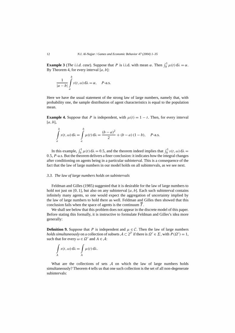
Example 3 (The i.i.d. case). Suppose thatP is i.i.d. with meanα. Then∫ 1

0 µ(t)dλ = α.By Theorem 4, for every interval[a, b]:

1

|a − b|b∫a

s(t,ω)dλ= α, P -a.s.

Here we have the usual statement of the strong law of large numbers, namely thaprobability one, the sample distribution of agent characteristics is equal to the popumean.

Example 4. Suppose thatP is independent, withµ(t) = 1 − t . Then, for every interva[a, b],

b∫a

s(t,ω)dλ=b∫a

µ(t)dλ= (b− a)2

2+ (b− a) (1− b), P -a.s.

In this example,∫ 1

0 µ(t)dλ= 0.5, and the theorem indeed implies that∫ 1

0 s(t,ω)dλ=0.5,P -a.s. But the theorem delivers a finer conclusion: it indicates how the integral chafter conditioning on agents being in a particular subinterval. This is a consequencefact that the law of large numbers in our model holds on all subintervals, as we see

3.3. The law of large numbers holds on subintervals

Feldman and Gilles (1985) suggested that it is desirable for the law of large numbhold not just on[0,1], but also on any subinterval[a, b]. Each such subinterval contaiinfinitely many agents, so one would expect the aggregation of uncertainty impliethe law of large numbers to hold there as well. Feldman and Gilles then showed thconclusion fails when the space of agents is the continuumT .

We shall see below that this problem does not appear in the discrete model of thisBefore stating this formally, it is instructive to formulate Feldman and Gilles’s idea mgenerally:

Definition 9. Suppose thatP is independent andµ ∈ C. Then the law of large numbeholds simultaneously on a collection of subsetsA ⊂ 2T if there isΩ ′ ∈Σ , withP(Ω ′)= 1,such that for everyω ∈Ω ′ andA ∈A:∫

A

s(t,ω)dλ=∫A

µ(t)dλ.

What are the collections of setsA on which the law of large numbers holdsimultaneously? Theorem 4 tells us that one such collection is the set of all non-degesubintervals:


ture

surable,e s

t

resulttationshe law

of the

efinedegral

ers

Corollary 1. Suppose that P is independent with µ ∈ C , then the law of large numbersholds simultaneously on all subintervals.

It is easy to see that the law of large numbers does not hold simultaneously onall infinitesubsets, 2T .17 Theorem 4 and Corollary 1 thus illustrate the role of the interval structhatT inherits from the continuum.

3.4. The law of large numbers in the continuum

3.4.1. States, events, and probabilitiesWhen the space of agents is the continuumT = [0,1], we continue to useΩ = ST

as state space. However, to ensure that agents’ random characteristics are meawe enrich the set of events toΣ , the σ -algebra generated by the random variabls(t): t ∈ T . ThenΣ is the smallestσ -algebra of events with respect to which eachs(t),t ∈ T , is measurable.

A stochastic structure is a probability distributionP onΣ . SinceΣN ⊂ Σ ⊂ Σ , anysuchP defines, by restriction, probability distributions on the discrete modelsT andTN .As before, defineµ :T → [0,1] by µ(t)≡EP s(t).

Definition 10. A distribution P on (Ω,Σ) is independent if for every finite subset1, . . . , tK ⊂ T the random variable ss(t1), . . . , s(tK) are independent.

3.4.2. How should the law of large numbers be defined in the continuum?One would like to have an analogue of Theorem 4 for the continuum, namely a

asserting that the ‘average’ of a sample realization equals the integral of the expecalmost surely. How should such claim be stated? Recall the usual statement of tof large numbers in the standard case of an i.i.d. sequence of random variablesx1, . . .,namely that with probability 1;

limN→∞

1

N

N∑n=1

xn =Ex.

In the continuum, it is natural to replace averages by integrals, yielding a statementform

b∫a

s(t,ω)dλ=b∫a

µ(t)dλ, for every[a, b], P -a.s. (8)

The integral on the RHS represents the population mean and is always well-dwheneverµ ∈ C (an assumption we shall maintain throughout). The problem is the int

17 Example: letP be an i.i.d. process with mean 0.5, andΩ ′ a set ofP -probability 1 for which theconclusion of Theorem 4 holds. Obviously,(1/λ(A))

∫Aµ(t)dλ = 0.5 for everyA ⊂ T . For ω ∈ Ω define

Aω = t ∈ T : s(t,ω) = 0. Then, for everyω ∈ Ω ′ , (1/λ(Aω))∫Aω

s(t,ω)dλ = 0. Thus, for everyω ∈ Ω ′,the law of large numbers fails on some subsetAω of T . The example in fact proves that the law of large numbfails to hold simultaneously even on the collection of sets with well-defined frequencies.


gueowintegralis an

ace oftsw

in theodel is

n, anyisample

of the sample realizations, “∫ ba s(t,ω)dλ”. One is tempted to define this as the Lebes

integral of the sample realizationt → s(t,ω). From the literature (see Section 4), we knthis to be problematic because a typical sample realization is not measurable so thisis not meaningfully defined. In Section 4, I argue that this lack of measurabilityinevitable feature of the continuum, one with important substantive implications.

One solution suggested by the framework of this paper is to replaceλ with λ in the LHSof Eq. (8), obtaining:

b∫a

s(t,ω)dλ=b∫a

µ(t)dλ P -a.s.

That is, we look at the integral of the sample realization on a discretization of the spagents. Note that, althoughs(·,ω) is defined on all ofT , it is averaged out only over poinin the discretizationT , and the a.s. statement is made with respect to the probability laP

on the continuum.18

3.4.3. Main resultTheorem 5. For every independent P with µ ∈ C, any discretization T , and any interval[a, b]:

b∫a

s(t,ω)dλ=b∫a

µ(t)dλ, P -a.s. (9)

In particular,

b∫a

µ(t)dλ= limN→∞

b∫a

s(t,ω)dλN, P -a.s. (10)

That is, although a typical sample realization does not have a well-defined integralcontinuum, it has, nonetheless, considerable structure: its integral in the discrete mwell-behaved and satisfies the law of large numbers .

Note that the theorem asserts that this procedure works for any discretizatiointerval, and any independent probability law withµ ∈ C. Finally, Eq. (10) states that this the ‘right’ integral in the sense that this is what we get by looking at averages of srealizations in finite but increasingly large discrete models.

3.5. The Pettis integral and the law of large numbers

For two random variablef,f ′ on (Ω,Σ), define their inner product as(f | f ′) =∫Ω f · f ′ dP = cov(f,f ′) + EfEf ′. Also, f andf ′ are equivalent if they agree with

probability 1. The following definition is standard.19

18 This makes sense since any such law induces a law in the model where the set of agents isT .19 Diestel and Uhl (1977) is a basic reference.


on 5).tationt cleare

al that

tinuum

r thehisbelow

s is not

ents

to

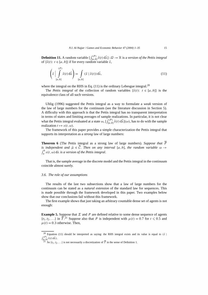
Definition 11. A random variable[∫ (P )[a,b] s(t)dλ] :Ω → R is aversion of the Pettis integralof s(t): t ∈ [a, b] if for every random variablex,

(x

∣∣∣(P )∫

[a,b]s(t)dλ

)=∫

[a,b](x | s(t))dλ, (11)

where the integral on the RHS in Eq. (11) is the ordinary Lebesgue integral.20

The Pettis integral of the collection of random variabless(t): t ∈ [a, b] is theequivalence class of all such versions.

Uhlig (1996) suggested the Pettis integral as a way to formulate aweak version ofthe law of large numbers for the continuum (see the literature discussion in SectiA difficulty with this approach is that the Pettis integral has no transparent interprein terms of states and limiting averages of sample realizations. In particular, it is nowhat the Pettis integral evaluated at a stateω, [∫ (P )[a,b] s(t)dλ](ω), has to do with the samplrealizationt → s(t,ω).

The framework of this paper provides a simple characterization the Pettis integrsupports its interpretation as astrong law of large numbers:

Theorem 6 (The Pettis integral as a strong law of large numbers).Suppose that Pis independent and µ ∈ C. Then on any interval [a, b], the random variable ω →∫ ba s(t,ω)dλ is a version of the Pettis integral.

That is, the sample average in the discrete model and the Pettis integral in the concoincide almost surely.

3.6. The role of our assumptions

The results of the last two subsections show that a law of large numbers focontinuum can be stated as anatural extension of the standard law for sequences. Tis made possible through the framework developed in this paper. Two examplesshow that our conclusions fail without this framework.

The first example shows that just taking an arbitrary countable dense set of agentenough:

Example 5. Suppose thatΣ andP are defined relative to some dense sequence of agt1, t2, . . . in T .21 Suppose also thatP is independent withµ(t) = 0.7 for t 0.5 andµ(t)= 0.3 otherwise. Then,

20 Equation (11) should be interpreted as saying: the RHS integral exists and its value is equal(x |∫ (P )[a,b] s(t)dλ).21 Sot1, t2, . . . is not necessarily a discretization ofT in the sense of Definition 1.


f largeges butt even

ace of

s)

ils. In

emitingThiss

in theditionalin

ven

her

(1) The dense sequence of agentst1, t2, . . . may be chosen so that, for almost everyω,limN→∞ 1

N

∑Nn=1 s(tn,ω) exists but is different from 0.5;

(2) The dense sequence of agentst1, t2, . . . may be chosen so that, for almost everyω,limN→∞ 1

N

∑Nn=1 s(tn,ω) does not exist.

The example illustrates that the way we build the discretizing sequenceTN in Definition 1is critical: a dense sequence of agents can be found so the conclusion of the law onumbers can fail either because sample realizations have well-defined limit of averathis limit violates the law of large numbers, or because the limit of averages does noexist.

The second example shows that the use of finitely additive probabilities on the spagents is critical.

Example 6. Suppose thatQ is a dense subset ofT (for instance, the set of rationaland thatP is i.i.d. with mean 0.5. Letλ′ be anycountably additive probability measureonQ. Define the limiting averages underλ′ as: limN→∞

∑Nn=1λ

′(tn)s(tn,ω). Note that∫ 10 µ(t)dλ′ = 0.5.

Then there is a set of states,S ⊂Ω , with P(S) > 0, such that

1∫0

s(t,ω)dλ′ =1∫

0

µ(t)dλ′, for everyω ∈ S.

That is, the conclusion of the law of large numbers for the discrete model, Eq. (7), fafact, the RHS of the above equation is a constant 0.5 while the LHS is random.22

In this example, countable additivity forcesλ′ to put most of its weight on a large finitset of points. Since the average outcome on any finite set of points is random, the liaverage underλ′ will also be random and the law of large numbers cannot hold.problem does not arise in our construction because the density chargeλ assigns zero masto any finite set of points.

3.7. Correlation

Our analysis extends to cover the type of correlated processes frequently usedliterature, namely processes where individual characteristics are independent conon a common aggregate parameter. To make this formal, let(Ω,Σ) be the state spaceSection 3 and letΘ = θ1, . . . , θK be a finite set of aggregate parameters. For everyθ ∈Θlet Pθ be a probability distribution onΩ . We shall writeµθ ≡EPθ s(t).

22 To see this, arrange the elements ofQ in any weakly decreasing order relative to the weights giby λ′ . Fix 0< ε < 0.5; countable additivity implies that we can findN large enough thatλ′(t1, . . . , tN ) 1 − ε. Consider the positive probability eventΩ ′ that s(tn,ω) = 1 for 1 n N . For any ω ∈ Ω ′,lim infN→∞

∑Nn=1λ

′(tn)s(tn,ω) 1 − ε. Thus, on a positive probability event, the limiting average is eitundefined, or different from the population mean.


t

hgiven

e

equal

of thelue may

tic isrs.

n the

flierstatedd.

undrge

Definition 12. P is conditionally independent if there is a probability distributionν onΘsuch that for everyS ∈Σ , P(S)=∑

θ Pθ (S)ν(θ) and for everyθ ∈Θ, Pθ is independen

with µθ ∈ C.

An example of how correlation may arise is the case whereP is“exchangeable:” eacPθ is i.i.d. with meanαθ , and these means are distinct. Realizations are independentknowledge of the value ofθ . Without this knowledge, however, learning the outcomes(t)

is informative about the underlying aggregate parameterθ and hence informative about thrandom outcomes(t ′) of some other agentt ′.

Theorem 7 (Strong law of large numbers in the correlated case).Suppose that P isconditionally independent. Then for P × ν-almost every (ω, θ):

b∫a

s(t,ω)dλ=b∫a

µθ (t)dλ, for every [a, b]. (12)

As in the independent case, the integral of the sample realization is almost surelyto the population mean. The difference is that now the population mean

∫ baµθ (t)dλ is itself

random, and so unknown ex ante. All we can say is that, almost surely, the integralsample realizations takes the same value as the population mean, whatever that vabe.

3.8. Finite outcomes

Let S be an arbitrary finite set of characteristics. Then an agent’s characterisa random vectors(t) :Ω → S taking values inS. The results on the law of large numbeof Section 3 directly generalize. Here we only briefly sketch the changes to be made

The state space again isΩ = ST , i.e., the set of all functionsω : [0,1] → S, andΣis theσ -algebra onΩ generated by the random variabless(t) : t ∈ T . Randomness incharacteristics is represented by a probability distributionP on (Ω,Σ).

Let∆ denote the unit simplex representing the set of all probability distributions ofinite setS. It is convenient to identifyS with the vertices of∆, sos(t) :Ω →∆. With thisnotation,µ(t)≡EP s(t) is a point in∆, representing the probability of each element oS.

The definition of C is the natural multi-dimensional generalization of our eardefinition. Then an analogue of Theorem 4 for the multi-dimensional case can beand proved exactly as before component by component. The obvious proof is omitte

4. Understanding the measurability problem

The difficulties in formulating a law of large numbers for the continuum revolve arowhether sample realizationst → s(t,ω) are measurable, and whether the law of la


85).stantivearacter

gents

teristicsity.

showscreteontoionsrsely.

ecall

of the

al iftion

ditional

numbers holds on all subintervals. See Judd (1985) and Feldman and Gilles (1923

This section addresses two questions: Does the measurability problem have a subcontent? And, why does not the discrete model, despite preserving much of the chof the continuum, suffer from the same problem?

4.1. Ex ante similarity vs. ex post variability

Economic models appealing to the law of large numbers typically assume that ahaveex ante similar characteristics, but that theirrealized characteristics display a degreeof stochastic independence. A good example is the common assumption that characare independent and identically distributed, which is a strong form of ex ante similar24

One way to formalize ex ante similarity is to require that thedistribution ofcharacteristics be piecewise uniformly continuous. Theorem 9 in Section 4.2 belowthat, under this interpretation of similarity of characteristics, the continuum and dismodels haveidentical similarity structures: there is a natural, essentially one-one andcorrespondence betweenC andC. This means that any of the commonly used specificatof distributions in the continuum can be translated to the discrete model, and conve

The problem is that independence requiresex ante similar agents to be wildlydissimilarex post. It is here where the discrete and continuum models are strikingly different. Rthe formulation of the law of large numbers in the continuum Eq. (8) as:

b∫a

s(t,ω)dλ=b∫a


As discussed earlier, this is not meaningful because∫ bas(t,ω)dλ is not well-defined. In

the discrete model, by contrast, Theorem 4 provides a straightforward formulationlaw of large numbers:

b∫a

s(t,ω)dλ=b∫a


Why does Eq. (14) make sense, while Eq. (13) does not?

23 Here is a brief formal statement of the problem. Consider an i.i.d. process with meanα, and letP denotethe joint distribution on the state spaceΩ . Judd pointed out that the set of sample realizationst → s(t,ω) isnon-measurable with respect toΣ . Say thatt → s(t,ω) satisfies the law of large numbers on every subinterv1/(a − b)

∫ ba s(t,ω)dλ = α on every subinterval[a,b]. Feldman and Gilles showed that any sample realiza

must be either non-measurable or does not satisfy the law of large numbers on every subinterval.24 Correlation does not remove the problem in the continuum, provided that some degree of con

independence remains (as in Section 3.7, for instance).


. (13)ly

e and

hown

n thatns and

risticssufferi.i.d.t raisections,nsible, but

ed bygrate

abilitymon as-eristicstypes,

In mod-anisme is noagents.ies re-divid-

llowing

, 1968).

We first note that, for a fixedω, a sample realizationt → s(t,ω) in the continuum isintegrable if and only if it is approximately continuous, in the sense that:25

inff∈C

∫T

∣∣s(t,ω)− f (t)∣∣dλ= 0. (15)

This means that any statement of the law of large numbers along the lines of Eqmakes the implicit requirement that agents’realized characteristics must be approximatecontinuous. This, in essence, is the point made by Feldman and Gilles (1985).

But there is a fundamental incompatibility between stochastic independencrequiring nearby agents to have similar characteristicsex post. This incompatibility is notan artifact of the continuum; in fact, it appears in full force in our discrete model, as sin the following result:

Theorem 8. Suppose that P is i.i.d. with mean α = 0.5. Then

inff∈C

∫T

∣∣s(t,ω)− f (t)∣∣dλ 0.5> 0 P -a.s.

The theorem says that the discrete model is no different from the continuum iindependence also requires an irreducible discrepancy between sample realizatiotheir best continuous approximations.

If the conflict between stochastic independence and continuity of realized characteis the same in the discrete model as in the continuum, why does not the formerfrom the measurability problem? Theorem 8 shows that a typical realization of anprocess cannot be approximated by a continuous function. This, however, does nothe same problems in the discrete model because we identified a broad class of funF ⊃ C, that are not approximately continuous, but nevertheless have a perfectly seintegral. Roughly, the discrete model inherits the similarity structure of the continuumnot its inability to integrate complicated functions (ones that cannot be approximatcontinuous functions). In the continuum, by contrast, the only functions we can inteare those that are approximately continuous.

The other question raised at the beginning of this section is: Does the measurproblem have a substantive content? Needless to say, independence is a very comsumption in economic models; models with ex ante identical agents whose charactare determined by independent random draws (representing wealth, information,etc.) abound. Independence in these models often plays a crucial, substantive role.els with a finite number of agents, including auctions, public goods and other mechdesign problems, dropping independence may drastically alter the analysis. Therreason to expect independence to be less critical in models with a large number ofIn summary, extending the models of Information Economics to study large economquires that one reconciles two conflicting goals: to be able to aggregate (integrate) inual choices and outcomes into economy-wide aggregates while, at the same time, a

25 In fact, approximation can be obtained using only continuous functions (see, for instance, RoydenWe use the classC for expository convenience.


stantiveof the

backunique

d

etweenl. The

s thatals. In

onlyted. As

for stochastic independence of characteristics. The measurability problem has subrather than purely technical content in so far as it is the mathematical consequenceimpossibility of reconciling aggregation and independence in the continuum.

4.2. Piecewise uniformly continuous functions on T and T coincide

Here we show that piecewise uniformly continuous functions can be ‘transferred’and forth between the continuum and the discrete model. This transfer is essentiallyand preserves integration.

4.2.1. Transfers between C and CThediscretization of f ∈ C is the functionf :T → R given byf (t)= f (t), ∀t ∈ T . In

this case, we also refer tof as anextension of f . Starting withf ∈ C, its discretizationfmust be inC. Conversely, givenf ∈ C and a component interval(am−1, am) ∩ T , f hasa unique continuous extension to the interval[am−1, am] in the continuum.26 This definesa unique piecewise uniformly continuous extensionf :T → R, except possibly at the enpointsam, m= 1, . . . ,M, where we setf arbitrarily. The resultingf is uniquely definedup to a finite set of points (which has measure zero under bothλ andλ). We thus have:

Theorem 9. For any f ∈ C, its discretization f belongs to C . Conversely, any f ∈ C hasan essentially unique extension f ∈ C: if f1, f2 are two such extensions, then f1(t)= f2(t)

for t ∈ T except for at most finitely many points.

4.2.2. Transfer preserves integrationTheorem 9 establishes a natural and essentially one-to-one correspondence b

piecewise uniformly continuous functions in the continuum and the discrete modenext result shows that this correspondence preserves integration:

Theorem 10. For any f ∈ C,

b∫a

f dλ=b∫a

f dλ on any interval [a, b].

4.2.3. How rich is C?The class of piecewise uniformly continuous functions is clearly an important clas

includes all continuous functions and all step functions that are constant on interva sense,C is as rich a class of functions on the continuum as one can hope for. The(bounded) functions tractable enough in the continuum are those that can be integrawe pointed out earlier, the integrability of (a bounded function)g :T → R implies

inff∈C

∫T

∣∣g(t)− f (t)∣∣dλ= 0. (16)

26 See, for instance, Royden, 1968, Proposition 11, p. 136.


at aremaying we

l as the

ampleiffers

osedh timeso the

finiteithof the

iformly

y ofonomicd forthor the

f largetegralsurely.

g step)

Thus, in the continuum the only function that can be used in practice are those thapproximately piecewise uniformly continuous in the sense of Eq. (16). Theorem 9be loosely interpreted to mean that, up to closure, the discrete model captures anythcan deal with in the continuum.

5. Related literature

I briefly discuss the differences with three closely related approaches.

5.1. The sampling approach

Bewley (1986) and Guesnerie (1981, 1995) proposed that one defines the integralimiting average over a randomly drawn infinite sample of agentst1, . . ..

One way to think of our discretizing sequence is that it represents a typical sof agents drawn from the continuum. The approach proposed in this paper dfundamentally from the sampling approach, however: We choose afixed set of agentsT as our primitive. We want the same set to worksimultaneously for all functions andprobability distributions we build on it subsequently. In the sampling approach propby Bewley and Guesnerie, one draws a random sample from the continuum eacan integral is to be evaluated. The underlying model then is the continuum, anddifficulties this model raises are not circumvented.

5.2. Countable models

Another approach, pioneered by Feldman and Gilles (1985), is to take an insequence of agentst1, . . . and define a density charge on it. The major difference wthe discrete model developed in this paper is that the latter preserves key featurescontinuum. The metric and interval structures are preserved, as well as piecewise uncontinuous functions and their integrals.27

The fact that our discrete model is continuum-like means that it enjoys manthe features that make continuum models tractable and convenient to use in ecapplications. It also means that intuitions and insights can be translated back anbetween continuum and discrete models, using whichever is more convenient fspecific application at hand.

5.3. Linear methods

Uhlig (1996) proposed the use of the Pettis integral as a way to formulate the law onumbers in the continuum. Using this approach, Uhlig (1996) shows that the Pettis inof an i.i.d. process is a random variable that equals the population mean almost

27 Theorems 9 and 10 provide a one-to-one mapping between piecewise uniformly continuous (includinfunctions in the continuum and the discrete model that preserves integration.


posedtypicalmon to

Indeed,mplems toained

s in thetegral of

a law, state-e

ructureen the

to1989)public

r ouroblemproveand

ublic

Al-Najjar (1995) showed that stochastic processes on the continuum can be decominto aggregate and idiosyncratic components, and that the limiting average on asample converges to the aggregate component of the process. The approach comboth papers is to convert the original stochastic process to anL2-valued mapping onT (byviewing each random variable as a vector inL2). See Section 3.5 for details.

A difficulty with this formulation is that once a stochastic process is converted to aL2-valued mapping, the underlying state space no longer plays any role in the analysis.the definition of the Pettis integral has no immediate interpretation in terms of sarealizations, limiting averages, and so forth. Thus, although the Pettis integral seeprovide the intuitively correct answer, its interpretation as a law of large numbers remproblematic. By contrast, the present paper produces a strong law of large numbertraditional sense: we consider the sample path at each state and assert that the inthis path equals the population mean almost surely.

The discretization approach provides a new interpretation of the Pettis integral asof large numbers. Theorem 6 shows that the Pettis integral coincides almost surelyby-state, with the empirical frequencies ofany discretization of the continuum. As thexamples in Section 3.6 show, this interpretation is possible only because of the stintroduced in this paper (e.g., finitely additive density charges, the transfer betwediscrete and continuum models, etc.).

6. Application: mechanism design and public goods in large economies

In this final section, I illustrate the framework of this paper by applying ita mechanism design problem in a large economy with private information. Rob (and Mailath and Postlewaite (1990) considered the problem of externalities andgoods in a sequence of finite, but increasingly large models of agents.

The goal of this section is to use this familiar economic context to “test” whetheframework makes sense. In particular, I show that that this mechanism design prhas a straightforward formulation in a large, atomless public good economy. I thena sharp inefficiency result using the concept of ‘influence’ introduced in Al-NajjarSmorodinsky (1996).

6.1. The primitives

The space of agents isT . Each agent has a type represented by a valuation for the pgood in a finite setS = 0< s1 < · · ·< sM . We use as state space the setΩ = ST . Agents’random types are represented by a functions :T ×Ω → S. A ‘ ˜ ’ will denote a randomvariable when explicit reference toω is suppressed. As before, theσ -algebraΣ used is theone generated by all sets of the forms(t)= s, s ∈ S, t ∈ T .


wherelater).

ge

h lesssed in

the

never

modelsy littlepaper,

vision

Provision of the public good is modeled as a functionδ :Ω → 0,1, where the publicgood is provided iffδ = 1.28 Given a transferc ∈ R and a provision outcomeδ, the payoffof an agent of types is sδ− c.

We assume that types are independent; that there isα such thatP s(t)= 0> α > 0 foreveryt ; and thatt → P s(t)= s belongs toC for everys ∈ S.

6.2. Defining mechanisms

Appealing to the Revelation Principle, we focus on direct revelation mechanismseach agent reports his type (incentive compatibility constraints are introducedA mechanism in this context has two components. First, a mechanism includes aprovisionfunction δ :Ω → [0,1]. We make the obvious assumption that

δ is a random variable,29 (17)

a requirement also needed in finite models. Second, the mechanism includes atransferfunction:

c :T ×Ω → R,

so c(t,ω) is the transfer paid by agentt in stateω. At a minimum, we need the averaexpected transfer,

∫Ec(t,ω)dλ, to be well-defined. We thus require that:

for every agentt, c(t) is a random variable, (18)

so the expectationEc(t) is meaningful. We also require that:

the functiont →Ec(t) belongs toF , (19)

ensuring that∫Ec(t)dλ is well-behaved.

Conditions (18) and (19) are rather weak, and they are obviously needed. Mucobvious are the implications of the phenomenon of ‘disappearing mass’ discusSection 2.4.1. There we displayed a simple example of a functionf that is strictly positive,yet

∫f (t)dλ = 0 (Example 1). To appreciate the implications of this example on

problem of defining efficient mechanisms, letc′(t,ω)≡ c(t,ω)− f (t). Sincef is strictlypositive, every agent is strictly better off underc′ relative toc. But since

∫f (t)dλ= 0, the

aggregate payment collected underc′ is the same as underc.This example points out that without additional restrictions, optimal mechanisms

exist, since any mechanism can be improved by using a function likef to generate a‘money pump’ that increases every agent’s payoff. This, perhaps, is one reason whywith a countable number of agents and finitely additive measures received relativelinterest in the literature on large economies. Using the structure developed in thishowever, this problem is easily remedied by requiring:

the functiont → c(t,ω) belongs toF , P -a.s. (20)

We can now state our formal definition of a mechanism:

28 The choice ofST as state space here is not without loss of generality as it requires that public good proand transfers to agents depend deterministically on the vector of agents’ reports.

29 That is,δ :Ω → [0,1] isΣ -measurable.


il forma

ments

besign

ta costpost:

taking

Definition 13. A mechanism is a pair (δ, c), where δ is a provision function andc isa transfer function such that conditions (17)–(20) hold.

An obvious requirement is that the expected value of aggregate transfer,∫ ba c(t,ω)dλ,

is equal to the integral of the expected transfers:

E

b∫a

c(t,ω)dλ=b∫a

Ec(t,ω)dλ, for every[a, b]. (21)

This amounts to a version of Fubini’s theorem. In general, Fubini’s Theorem may fafinitely additive probabilities (see, for instance, Marinacci, 1997). The following lemshows that Fubini’s Theorem holds for mechanisms satisfying the rather mild requirein Definition 13.

Lemma 1. Let c :T ×Ω → R be any bounded function satisfying conditions (18)–(20).Then Eq. (21) holds on every interval [a, b].

6.3. Individual rationality and incentive compatibility

The conditions of (interim) individual rationality and incentive compatibility canformulated here in a way that is virtually identical to finite-agent mechanism deproblems:

Definition 14. The mechanism(δ, c) is individually rational (IR) if

sE(δ∣∣ s(t)= s

)−E(c(t)

∣∣ s(t)= s) 0 for all t ∈ T ands ∈ S. (22)

Definition 15. The mechanism(δ, c) is incentive compatible (IC) if for every t ∈ T ands, s′ ∈ S,

sE(δ∣∣ s(t)= s

)−E(c(t)

∣∣ s(t)= s) sE

(δ∣∣ s(t)= s′

)−E(c(t)

∣∣ s(t)= s′). (23)

6.4. Inefficiency in large public good economies with private information

We now consider the problem where producing the public good entails a per capiof β > 0. One way to formulate feasibility is to require that budget balance holds ex

1∫0

c(t,ω)dλ βδ(ω), P -a.s. (24)

A weaker requirement is that budget balance holds on average, which we obtain byexpectations of both sides of Eq. (24):

E

1∫c(t,ω)dλ βEδ. (25)

0


) and

esultsnomyajjar

ehe

ence,

o the

t

We refer to this condition as ex ante feasibility (see Mailath and Postlewaite, 1990interpret it as reflecting the availability of a risk-neutral lender.

We can now state our main inefficiency result:

Theorem 11. For any per capita cost β > 0, the probability of provision of the public goodis zero:

Pω: δ(ω)= 1

= 0,

under any mechanism (δ, c) satisfying incentive compatibility, individual rationality, andex ante feasibility.

The result is an atomless, large-economy version of the asymptotic inefficiency rin Rob (1989) and Mailath and Postlewaite (1990). Its proof appeals to a large-ecogeneralizations of the concepts of “influence” and “pivotalness” introduced by Al-Nand Smorodinsky (1996) and which are of independent interest.

6.5. Influence and non-pivotalness theorem in large economies

Rearrange the IC constraint, Eq. (23), to obtain:

E(c(t)

∣∣ s(t)= s)−E

(c(t)

∣∣ s(t)= s′) s

[E(δ∣∣ s(t)= s

)−E(δ∣∣ s(t)= s′

)]︸︷︷︸V

.

(26)

The termV above represents agentt ’s influence on the probability of provision as hchanges his report froms to s′. Following Al-Najjar and Smorodinsky (1996), define tinfluence of agentt relative toδ as:

V (t, δ)= maxs,s ′∈S

∣∣E(δ ∣∣ s(t)= s)−E

(δ∣∣ s(t)= s′

)∣∣.Equation (26) tells us that an agent’s expected contribution is bounded by his influV (t, δ). Note that one can always findδ under whichV (t, δ) is high for a particular agentt .For example, a ‘dictatorial’δ that ignores the reports of all but a particular agentt is anexample where one agent has large influence. The key point is thataverage influence mustbe zero for any choice ofδ.

Theorem 12. For any δ :Ω → [0,1],1∫

0

V (t, δ)dλ= 0.

The proof, found in Appendix A, adapts the argument in Al-Najjar and Smorodinsky tdiscrete modelT .30

30 Since every bounded function is integrable, the integral∫ 10 V (t, δ)dλ is always well defined. We are no

asserting, however, that the functiont → V (t, δ) belongs toF .


nt times

,

s likeether

thatn

ntegralbeing

n agente, theof an

the

ns inrestrict

these,ll as in0), onhave to

Proof of Theorem 11. Condition IR, Eq. (22), evaluated ats = 0 implies thatE(c(t) |s(t)= 0)= 0. Averaging over the types of agentt , Eq. (26) implies

Ec(t) sMV(t, δ). (27)

This says that the expected contribution of any agent is bounded above by a constathe maximum influence of that agent underδ. Integrating overT , we obtain

1∫0

Ec(t)dλ sM

1∫0

V(t, δ)dλ. (28)

From Eq. (28) and Theorem 12, we have∫ 1

0 Ec(t)dλ = 0. From ex ante feasibilityEq. (25),

Pω: δ(ω)= 1

≡Eδ 1

β

1∫0

Ec(t)dλ= 0.

6.6. Mechanism design and the law of large numbers

The law of large numbers is central to formulating mechanism design problemthe one described above. As an illustration consider the problem of verifying whfeasibility is satisfied. Such verification requires computing the integral:∫

T

c(t,ω)dλ. (29)

Our framework ensures that the value of this integral is well-behaved providedcondition (20) is satisfied. This condition requires thatc has well-behaved distributioand that

∫T c(t,ω)dλ is the limit of integrals in large finite models.

The contrast with the continuum should be emphasized: there, whether or not an ilike that in expression (29) is meaningful depends crucially on the mechanismconsidered. An important class of mechanisms for which the integral in (29)cannot bedefined is that of anonymous mechanisms. In such mechanisms, the transfer of adepends only on his type, not his label. With an i.i.d. distribution of types, for instancproblem of defining the integral in (29) reduces to that of integrating a typical drawi.i.d. process, which is not meaningful in the continuum.

This is not to say thatno mechanism is well defined in the continuum. Rather,question is:How severe a restriction do we need to impose on the class of allowablemechanisms? The example of anonymous mechanisms indicates that the restrictiothe continuum have to be very severe indeed. In the discrete model we also need tothe class of allowable mechanisms, namely by requiring conditions (17)–(20). Ofconditions (17) and (18) are innocuous, and are needed in the continuum as wemechanism design problems with a finite number of agents. Conditions (19) and (2the other hand, considerably weaken the measurability requirement that one wouldimpose in the continuum.


ngl). Butte. Theh to thefinite

ing

I alsoheir

mumao,

)

It may be possible to find anindirect way to use the continuum to model interestimechanism design problems in large economies (e.g., using the Pettis integraany such approach will have to forego references to what happens at each stadiscretization approach presented here has the advantage of being similar enougcontinuum, yet consistent with a straightforward large-economy formulation ofmechanism design problems.

Acknowledgments

This paper is dedicated to Marcel K. Richter. It will be reprinted in the forthcomvolumeFoundations of Economic Theory, Essays in Honor of Marcel K. Richter, Springer-Verlag.

I am grateful to an Associate Editor and a referee for their valuable feedback.thank Larry Blume, Jeff Ely, Massimo Marinacci, Rafi Rob, and Asher Wolinsky for tvaluable comments, and Lineu Vargas for proofreading earlier versions.

Appendix A

Proof of Theorem 1. Let l∞ denote the set of all bounded sequences with the suprenorm. That is, forx = (x1, . . .) ∈ l∞, ‖x‖ = supn xn. We use the fact (see Rao and R1983, p. 39–41) that there exists a functionT : l∞ → R that is:

(1) linear: T (cx + dy)= cT (x)+ dT (y);(2) non-negative: T (x) 0 if infn xn 0;(3) preserves identity: T (1,1,1, . . .)= 1;(4) translation invariant: T (x1, x2, . . .)= T (x2, x3, . . .).

Any such function is known as a Banach limit. The above reference shows that

lim infn

xn T (x) lim supn

xn;in particular,T (x)= limn→∞ xn whenever the limit exists. Thus, one may think ofT as ageneralized limit.

Fix one such functionT . For an arbitrary setA⊂X, define

λ(A)= T(λ1(A),λ2(A), . . .

).

It is clear thatλ thus defined is a finitely additive probability onX. Furthermore, Eq. (2must hold sinceT assigns to every convergent sequence its limit.Proof of Theorem 2. We drop reference the interval[a, b] in what follows to simplifynotation.

1. ThatF is non-decreasing follows from the additivity ofλ, so it only remains toshow thatF is right-continuous. Suppose thatr is a point at whichF is not right-continuous. Using the fact thatF is non-decreasing, there is a sequencern ↓ r such thatF(rn) ↓ F+ >F(r) supr ′<r F (r

′)≡ F−.


ed

n

t

pty)y.

iryayev

By the additivity of λ and Eq. (4), in Definition 4, we haveF(r) ≡ λf (t) r λf (t) = r + λf (t) r ′ ≡ (F+ − F−) + F(r ′) for any r ′ < r. For anyε > 0, thereis r ′ < r such thatF− − F(r ′) < ε. Thus, given anyε > 0 and choosingr ′ as in the lastsentence, we haveF(r) (F+ − F−) + F− − ε = F+ − ε, so F(r) = F+, which isa contradiction.

2. Change of variables. Sincef is bounded, we may restrict attention to some fixinterval[rmin, rmax], soF(rmin)= 0 andF(rmax)= 1. Chooser1, . . . , rM to be equallyspaced points such thatrmin = r0 < · · · < rM = rmax and consider the step functiogM : [rmin, rmax] → [rmin, rmax] that takes the constant valuerm on the interval(rm, rm+1].

Clearly, the sequence of simple functionsgM(f (·)) converges uniformly tof , soby the definition of the integral (Definition 3), we have limM→∞

∫ bagM(f (·))dλ =∫ b

a f (·)dλ.For any interval(rm, rm+1],m= 1, . . . ,M, we have:

1

|a − b|b∫a

χ(rm,rm+1](f (t)

)dλ(t)=

∫R

χ(rm,rm+1](r)dF(r).

By linearity of the integral, this extends to all step functionsgM constructed in the lasparagraph:

1

|a − b|b∫a

gM(f (t)

)dλ=

∫R

gM dF(r).

Taking limits of both sides asM goes to infinity establishes the claim.3. The integral is the limit of integrals in finite models. If f ∈ F then, by Definition 5,

FN(·)→ F(·) weakly. Clearly,∫ ba f dλN = ∫

Rr dFN(r), and by part (2) above,

∫ ba f dλ=∫

Rr dF(r). Weak convergence then implies that limN→∞

∫Rr dFN(r)=

∫Rr dF(r).

Proof of Theorem 3. It is enough to prove the claim for the case in whichf is uniformlycontinuous. We prove thatf has asymptotic frequencies; this then implies thatf doestoo. Sincef is continuous, we can find a countable set of disjoint (possibly emopen intervalsIk∞k=1 such thatI = t : f (t) > r = ⋃∞

k=1 Ik . Clearly, the boundarof I , denoted∂I , consists of the end points of the intervalsIk , and is thus countableIn particular,λ(∂I)= 0.

By definition,

1− FN(r)≡ λN (I) and 1− F(r)≡ λ(I ).

Using a standard characterization of weak convergence (see, for instance, Sh(1984), Theorem 1, p. 309), the sequence of measuresλN converges weakly toλ if andonly if for every measurable setA with λ(∂A) = 0, λN (A) → λ(A). In our case weakconvergence implies thatλN(I) → λ(I ). This impliesFN(r) → F(r) = F(r) for everyr ∈ R, and the result follows.31

31 This proves more than just weak convergence, which requires only convergence forr ’s that are continuitypoints ofF .


in

edakewhich

onhat

.hat

m 2,

Proof of Theorem 10. The result follows from the change of variables formulaTheorem 2.

To prove Theorem 4 we note that the assumptionµ ∈ C is unnecessary; the result (statbelow as Theorem 4*) holds forµ ∈F . We chose the more restrictive assumption to mit easier to compare this result with those for the continuum (Theorems 5 and 6 forfunctions inF\C do not make sense).

An example of a process withµ ∈ F\C is the following: Consider an i.i.d. processT that takes the values 1/3 and 2/3 with equal probability. Theorem 4 guarantees talmost every realization has the property that its integral is 0.5 on every subinterval[a, b].Let µ be one such realization, and note thatµ ∈ F\C (this follows from Theorem 8)The independent process with meanµ is the desired example. It is interesting to note tintegrals of sample realization on intervals cannot separate the process with meanµ fromthe 50-50 i.i.d. process.

Theorem 4*. Suppose that P is independent and µ ∈ F . Then for P -almost everyrealization ω, on every interval [a, b], the integral of the sample realization equals theintegral of the expectations.

Proof. Fix an interval[a, b]. Sinceµ ∈F , by Theorem 2,

b∫a

µ(t)dλ= limN→∞

1

#TN ∩ [a, b]∑

TN∩[a,b]µ(t).

Using the version of the strong law of large numbers in Shiryayev (1984, Theorep. 364), there is a setΩ [a,b] ⊂Ω with P(Ω[a,b])= 1 such that for everyω ∈Ω[a,b]

limN→∞

1

#TN ∩ [a, b]∑

TN∩[a,b]s(t,ω)= lim

N→∞1

#TN ∩ [a, b]∑

TN∩[a,b]µ(t)

which proves the claim for a single interval[a, b].DefineΩ ′ = ∩Ω[a,b], where the intersection is taken over all intervals[a, b] with

rational endpoints. Since there are countably many such intervals, we haveP(Ω ′) = 1,and the law of large numbers is satisfied simultaneously on every such interval inT .

To prove the general claim, let[a, b] ⊂ [0,1] be an arbitrary interval wherea, b areirrational. Consider any sequences of rational numbersan ↑ a andbn ↓ b and fix anystateω ∈Ω ′. Belonging toΩ ′ implies that

bn∫an

s(t,ω)dλ=bn∫an

µ(t)dλ

for everyn. To simplify notation, writeAn = [an, bn] − [a, b]. Then,

bn∫a

s(t,ω)dλ=b∫a

s(t,ω)dλ+∫s(t,ω)dλ and

n An


s

nt

dom

bn∫an

µ(t)dλ=b∫a

µ(t)dλ+∫An

µ(t)dλ;

substituting, we obtain:

b∫a

s(t,ω)dλ=bn∫an

µ(t)dλ−∫An

s(t,ω)dλ=b∫a

µ(t)dλ+∫An

µ(t)dλ−∫An

s(t,ω)dλ.

The claim now follows by noting that the term∫Anµ(t)dλ− ∫

Ans(t,ω)dλ goes to zero a

λ(An)= an − a + b− bn → 0. Proof of Theorem 5. By Theorem 10, we may replace

∫ ba µ(t)dλ in Eq. (9) by

∫ ba µ(t)dλ,

so this equation is equivalent to:

b∫a

s(t,ω)dλ=b∫a

µ(t)dλ P -a.s. (A.1)

Sinceλ puts unit mass onT , any pair of statesω,ω′ that agree onT must also satisfy∫ bas(t,ω)dλ = ∫ b

as(t,ω′)dλ. This means that the random variableω → ∫ b

as(t,ω) on

(Ω,Σ) is in factΣ-measurable. Thus, Eq. (A.1) also holdsP -a.s., and it is thus equivaleto:

b∫a

s(t,ω)dλ=b∫a

µ(t)dλ P -a.s.

This, of course, is true by Theorem 4.Proof of Theorem 6. Let x be any random variable. Then

(x

∣∣∣ b∫a

s(t)dλ

)=(

[x −Ex] +Ex

∣∣∣ b∫a

s(t)dλ

)

=(x −Ex

∣∣∣b∫a

s(t)dλ

)+(Ex

∣∣∣b∫a

s(t)dλ

)

By Theorem 4,∫ bas(t)dλ is constant almost surely, so its covariance with any ran

variable is zero. This andE[x −Ex] = 0 imply:(x −Ex

∣∣∣b∫s(t)dλ

)= cov

(x −Ex,

b∫s(t)dλ

)+E[x −Ex]E

b∫s(t)dλ= 0.

a a a


m 4,

ns

h

ion

On the other hand, from the definition of the Pettis integral, and again using Theore(Ex

∣∣∣b∫a

s(t)dλ

)=ExE

b∫a

s(t)dλ=Ex

b∫a

µ(t)dλ.

In summary, we have(x

∣∣∣b∫a

s(t)dλ

)=Ex

b∫a

µ(t)dλ. (∗)

Next we compute∫ ba(x | s(t))dλ. It is convenient to write

b∫a

(x | s(t))dλ=

b∫a

(x | [s(t)−Es(t)] +Es(t)

)dλ.

Since thes(t)’s are independent, the[s(t) − Es(t)]’s are orthogonal with boundedL2-norm. Then, for any enumeration oft1, . . . we must have

∑∞n (x | [s(tn)−Es(tn)])2<∞

(see Dunford and Schwartz, 1958, IV.4.10, p. 251). In particular, for everyε > 0,(x | s(t)−Es(t)) < ε for all but finitely many values oft . Then the sequence of functiofN , wherefN = (x | s(t) − Es(t)) if this value exceeds 1/N andfN = 0 otherwise,converges to the functiont → (x | s(t) − Es(t)) uniformly. Furthermore,

∫ ba fN dλ = 0.

By the definition of the integral (Definition 3), we have:

b∫a

(x | s(t)−Es(t)

)dλ= 0.

On the other hand,(x |Es(t))=Ex Es(t). Combining these facts, we have

b∫a

(x | s(t))dλ=Ex

b∫a

Es(t)dλ. (∗∗)

Combining (∗) and (∗∗), we obtain(x

∣∣∣ b∫a

s(t)dλ

)=

b∫a

(x | s(t))dλ

which is the desired conclusion, Eq. (11).Proof of Theorem 7. The result follows since, by Theorem 4, Eq. (12) holds for eacθthat has positive probability.Proof of Theorem 9. Clearly, the restriction of a piecewise uniformly continuous functf :T → R is a function that is piecewise uniformly continuous onT .


t

valsn of

p

m

d to

l

e

In the other direction, fix a functionf that is piecewise uniformly continuous onT .Consider any interval(am, am+1) ∩ T on whichf is uniformly continuous. Thenf hasa unique continuous extension to the closure of this interval inT , namely[am,am+1].Repeating this process for allm, we obtain a uniquely defined functionf on theset T − a1, . . . , aM. The result follows by definingf arbitrarily on the finite sea1, . . . , aM. Proof of Theorem 8. Let g be a step function (i.e., constant on the component inter(am, am+1). Let s(t,ω) be a typical sample realization (i.e., satisfies the conclusioTheorem 4). On each componentAm that has positive mass and whereg assumes thevaluegm, we have

1

λ(Am)

∫Am

∣∣s(t,ω)− g(t)∣∣dλ= 0.5∗ [|1− gm| + |gm|] 0.5.

Clearly,∫T |s(t,ω)− g(t)|dλ 0.5.

Next, consider now any functionf ∈ C. Clearly, for everyε > 0, we can find a stefunctiong that is uniformlyε-close tof . Then

0.5∫T

∣∣s(t,ω)− g(t)∣∣dλ

∫T

[∣∣s(t,ω)− f (t)∣∣+ ∣∣f (t)− g(t)

∣∣]dλ

=∫T

∣∣s(t,ω)− f (t)∣∣dλ+

∫T

∣∣f (t)− g(t)∣∣dλ

∫T

∣∣s(t,ω)− f (t)∣∣dλ+ ε.

That is,∫T

|s(t,ω) − f (t)|dλ 0.5 − ε, for everyε > 0, and the claim of the theorefollows. Lemma A.1. Suppose that f :T → R is any function in F such that λt : f (t) < 0 = 0and λt : f (t) > 0> 0. Then

∫[0,1] f dλ > 0.

Proof. In what follows, references to[a, b] are suppressed and the interval is assumebe[0,1]. Condition (4) states that for everyr,

λ(f−1(r)

)= infr ′>r

F (r ′)− supr ′<r

F (r ′).

The assumptionλt : f (t) < 0 = 0 implies supr ′<0F(r′)= 0. Further,λt : f (t) > 0> 0

implies thatλ(f−1(0)) < 1. Thus, for somer ′ > 0, F (r ′) < 1. The result now follows bythe change-of-variables part of Theorem 2.Lemma A.2. For any allocation x , the function ω → ∫ b

ac(t,ω)dλ isΣ-measurable (hence

a random variable on (Ω,Σ)).

Proof. Note that∫ ba c(t,ω)dλN is a finite sum for any stateω, anyN and any subinterva

[a, b]. This means that the functionω → ∫ bc(t,ω)dλN is Σ-measurable. By th

a


re

ctionssenated

urndifyppeal

assumption that forP -almost every stateω, the functionω → c(t,ω) belongs toF ,Theorem 2 implies that for almost every state,

limN→∞

b∫a

c(t,ω)dλN =b∫a

c(t,ω)dλ.

Thus, the sequence of measurable functions∫ ba c(t,ω)dλN converges almost everywhe

to the function∫ bac(t,ω)dλ, implying that this is aΣ-measurable function as required.

Proof of Lemma 1. Note that∫ bac(t,ω)dλN is a finite sum for any stateω, anyN and

any subinterval[a, b]. Thus,

E

b∫a

c(t,ω)dλN =b∫a

Ec(t,ω)dλN.

By our assumption thatt →Ec(t,ω) belongs toF , we have limN→∞∫ ba Ec(t,ω)dλN =∫ b

aEc(t,ω)dλ. Taking limits, we obtain:

limN→∞E

b∫a

c(t,ω)dλN =b∫a

Ec(t,ω)dλ.

So it only remains to show that

limN→∞E

b∫a

c(t,ω)dλN =E

b∫a

c(t,ω)dλ.

From the proof of Lemma A.2, we know that the sequence of measurable fun∫ ba c(t,ω)dλN converges almost everywhere to

∫ ba c(t,ω)dλ (both viewed as function

of ω, of course). Furthermore, this sequence is dominated by a constant sincc isbounded by assumption. The claim of the Lemma now follows by applying the DomiConvergence Theorem.

The proof of Theorem 12 follows easily from the following lemma, which in tfollows from Theorem 1 in Al-Najjar and Smorodinsky (1996). Essentially, we mothe problem to an equivalent problem with a finite number of agents where we can ato the results Al-Najjar and Smorodinsky established for finite agent environments.

Lemma A.3. For every α > 0, there is a number K∗α such that for any δ :Ω → [0,1], no

more than K∗α agents have influence exceeding α.

Proof. For a fixed, finite set ofK agents,T ′, define

δ′ :∏

′S → [0,1]

t∈T


thiginal

er

ve

ory 92,

bles.

7–159.mers.

erard

Econ.

le des

ry 35,

2.Econ.

as follows: for a vector of types of agents inT ′, s(t): t ∈ T ′,δ′(s(t)= s(t): t ∈ T ′)=E

(δ∣∣ s(t)= s(t): t ∈ T ′).

Note that fort ∈ T ′, V (t, δ) = V (t, δ′). Thus,δ′ is a mechanism in an environment wia finite set of agentsT ′, and where each agent has the same influence as in the orproblem.

Suppose the claim of the lemma were false. Then there isα > 0 such that forevery K > 0 there is a finite setT ′ of K agents such thatV (t, δ) > α for everyt ∈ T ′. From the observation made in the last paragraph, we have a mechanismδ′ ina finite environmentT ′ such thatV (t, δ′) > α for agents inT ′. In particular, averaginfluence, 1/K

∑t∈T ′ V (t, δ′) > α. This is a contradiction with Theorem 1 in Al-Najja

and Smorodinsky (1996) which states that average influence goes to 0 asK goes to infinity,uniformly over all mechanisms and all distribution of signals whereP s(t) = s > ε foreveryt ands. Proof of Theorem 12. Define the functionfN :T → R by fN(t) = V (t, δ) for t ∈ TN ,andfN (t)= 0 otherwise. From the lemma, it follows that givenα > 0 there isN such thatV (t, δ) < α for everyt /∈ TN . This implies that the sequence of functionsfN convergesto t → V (t, δ) uniformly. From the definition of the integral (Definition 3), we ha∫ 1

0 fN (t)dλ→ ∫ 10 V (t, δ)dλ asN → ∞. On the other hand,

∫ 10 fN(t)dλ= 0 for everyN ,

and the result follows.

References

Al-Najjar, N., Smorodinsky, R., 1996. Pivotal players and the characterization of influence. J. Econ. The318–342.

Al-Najjar, N.I., 1995. Decomposition and characterization of risk with a continuum of random variaEconometrica 63, 1195–1224. Corrigendum: Econometrica 67 (1999), 919–920.

Armstrong, T., Richter, M., 1984. The core–Walras equivalence. J. Econ. Theory 33, 116–151.Armstrong, T., Richter, M., 1986. Existence of nonatomic core–Walras allocations. J. Econ. Theory 38, 13Bewley, T., 1986. Stationary monetary equilibrium with a continuum of independently fluctuating consu

In: Hildenbrand, W., Mas-Colell, A. (Eds.), Contributions to Mathematical Economics: In honor of GDebreu. North-Holland, New York.

Diestel, J., Uhl, J., 1977. Vector Measures. In: Math. Surv., vol. 15. AMS, Providence, RI.Dunford, N., Schwartz, J., 1958. Linear Operators, Part I. Interscience, New York.Feldman, M., Gilles, C., 1985. An expository note on individual risk without aggregate uncertainty. J.

Theory 35, 26–32.Fishburn, P., 1970. Utility Theory for Decision Making. Wiley, New York.Gilboa, I., Matsui, A., 1992. A model of random matching. J. Math. Econ. 21, 185–197.Guesnerie, R., 1981. On taxation and incentives: further reflections on the limits of redistribution. Éco

hautes études en sciences sociales.Guesnerie, R., 1995. A Contribution to the Pure Theory of Taxation. Cambridge Univ. Press, Cambridge.Judd, K.L., 1985. The law of large numbers with a continuum of i.i.d. random variables. J. Econ. Theo

19–25.Khan, M., Sun, Y., 1999. Non-cooperative games on hyperfinite Loeb spaces. J. Math. Econ. 31, 455–49Mailath, G., Postlewaite, A., 1990. Asymmetric information bargaining problems with many agents. Rev.

Stud. 57, 351–367.Marinacci, M., 1997. Finitely additive and epsilon Nash equilibria. Int. J. Game Theory 26, 315–333.


t LLN.

Rao, K., Rao, M., 1983. Theory of Charges. Academic Press, New York.Rob, R., 1989. Pollution claim settlements under private information. J. Econ. Theory 47, 307–333.Royden, H.L., 1968. Real Analysis, 2nd Edition. MacMillan, New York.Shiryayev, A.N., 1984. Probability. Springer-Verlag, New York.Sun, Y., 1998. A theory of hyperfinite processes: The complete removal of individual uncertainty via exac

J. Math. Econ. 29, 419–503.Uhlig, H., 1996. A law of large numbers for large economies. Econ. Theory 8, 41–50.Weiss, E.A., 1981. Finitely additive exchange economies. J. Math. Econ. 8, 221–240.Werner, J., 1997. Diversification and equilibrium in securities markets. J. Econ. Theory 75, 89–103.

Documents

Aggregation and the law of large numbers in large economies