Working Paper

BANK OF GREECE

AGGREGATE SUPPLY AND DEMAND, THE REAL EXCHANGE RATE AND

OIL PRICE DENOMINATION

Yiannis Stournaras

No. 26 July 2005

AGGREGATE SUPPLY AND DEMAND, THE REAL

EXCHANGE RATE AND OIL PRICE DENOMINATION

Yiannis Stournaras

Bank of Greece and University of Athens

ABSTRACT

In an aggregate supply, aggregate demand model of an open economy with imperfect

competition in labour and product markets, the effectiveness of monetary and fiscal policies

depends on the degree of wage indexation, the exchange rate regime and the currency

denomination of the international prices of raw materials, such as oil. In a two country world

with a floating exchange rate, real consumer wage rigidity and the prices of imported raw

materials fixed in the currency of Country 2, monetary policy is effective only in Country 2,

but fiscal policy is relatively more effective in Country 1. These results may explain certain

characteristics and have certain implications for economic policy in the US and the Eurozone.

Keywords: Open economy macroeconomics, real exchange rate, oil price denomination

JEL classification: F41,Q43

Acknowledgements: I wish to thank participants in research seminars in the Economic Research Department,

Bank of Greece and in the Department of Economics, University of Athens for their useful comments.

Particularly I wish to thank Vassilis Droucopoulos and George Krimpas for insightful suggestions and a useful

discussion on the subject.

Address for Correspondence:

Yiannis Stournaras,

Economic Research Department,

Bank of Greece, 21 E. Venizelos Ave.,

102 50 Athens, Greece,

Tel.: + 30 210-320 3604

E-mail: stournaras@grmail.com

5

1. Introduction

The effectiveness of fiscal and monetary policies in open economies continues to be a

central issue in macroeconomics. The analytical framework is provided mainly by the

Mundell-Fleming-Dornbusch model (see, among others, Mundell, 1968; Dornbusch, 1980;

McCallum, 1996; Heijdra and Van der Ploeg, 2002). In recent years, many authors use the

new open economy macroeconomics model to tackle the same questions (Obstfeld and

Rogoff, 1996, chapter 10; Obstfeld, 2001; Lane, 2001).

The formation of EMU and the prospective participation of the enlargement countries

has revived interest in the economics of optimum currency areas, the choice of exchange rate

regime and the coordination of economic policies (see, among others, de Grauwe, 2001; Buti,

2003). One of the main conclusions of the theory of optimum currency areas is that the

choice of exchange rate regime and the effectiveness of monetary policy depends critically on

the nature of wage formation (Ishiyama, 1975; Edwards, 1989; Masson and Taylor, 1992;

Buiter, 1999). Those who argue in favour of flexible exchange rates, including Friedman

(1953), want to retain exchange rate flexibility as an instrument of adjustment in a world of

sticky nominal prices and wages. However, the presence of real rigidities implies that

nominal variables, such as the nominal exchange rate, play no role in the adjustment of

output and the real exchange rate.

In the present paper we develop a model to deal with certain of the above issues. In

Moschos and Stournaras (1998) an aggregate supply relationship was derived in a model of

an open economy with imperfect competition in its labour and product markets. This

relationship was used for an empirical investigation of real wage rigidity in Greece in order to

examine whether the loss of the exchange rate instrument (following Greece’s participation in

EMU) would imply a real cost or not. In the present paper, this aggregate supply relationship

is developed further and is combined with an aggregate demand one, derived from traditional

IS – LM equations under perfect capital mobility. Within this framework we investigate the

effectiveness of (ad hoc) monetary and fiscal policies under fixed and flexible exchange rates

and under complete consumer wage indexation (real consumer wage rigidity) and incomplete

wage indexation (nominal wage rigidity). We also investigate the effects of an adverse

supply-side shock (such as an increase in the international oil price) as well as the effects of

benign changes in market structure (the wage pressure parameter and/or the mark-up

coefficient), technology or the labour force. An interesting implication of the analysis is that

fixing the international raw material prices in the home currency introduces an element of

6

nominal inertia even under real consumer wage rigidity. In effect, the supply relationship

under nominal wage rigidity is qualitatively similar to the supply relationship under real wage

rigidity but with the international raw material prices fixed in the home currency.

We extend the analysis to a two-country world, under a floating exchange rate, real

consumer wage rigidity in both Country 1 and Country 2, and the price of imported raw

materials fixed in the currency of Country 2. In effect, Country 1 is characterized by real

rigidity, while Country 2 by nominal rigidity.

Within such a framework, an expansionary monetary policy in Country 1 has no

effect on output. An expansionary monetary policy in Country 2 has a positive effect on both

countries’ output through a reduction in the “world” interest rate. An expansionary fiscal

policy in Country 1 is more effective than an expansionary fiscal policy in Country 2: the

appreciation of Country 2’s exchange rate as a result of an increase in its government

expenditure, combined with nominal rigidity due to the fixing of raw material prices in its

currency, mitigates the initial effect of increased government expenditure on output since it

shifts its aggregate supply curve to the left.

If it is true that the Eurozone is characterized by real rigidities and the US by nominal

rigidities (the international pricing of raw materials in US dollars is one reason, the nature of

wage adjustment might be another – see Branson and Rotemberg, 1980; Nickell, 1997), our

analysis suggests that the Fed is in a position to affect “world” output but the ECB is not and

that Eurozone government expenditure is more effective as an instrument to affect output

compared to US government expenditure. The present two-country model and its results

extend in many ways those of Branson and Rotemberg (op. cit.), as well as Heijdra and Van

der Ploeg (op. cit. chapter 11), who examine the impact of monetary and fiscal policy under

different assumptions about wage formation in the two countries.

We do not attempt to justify the choice of this well-known aggregate supply, Mundell

– Fleming, IS - LM model as a framework of analysis (see, among others, Carlin and Soskice

(1990), who also use an imperfect competition framework, similar in spirit to the present

one). We do not attempt either to stress its differences and similarities with the new open

economy macroeconomics (Obstfeld, op. cit. and Walsh, 2003, chapter 6 might be useful

references for comparisons).

At the methodological level, we do not examine monetary and fiscal policies within

an explicitly utilitarian, intertemporal framework: our emphasis is on how supply-side

7

characteristics affect the relative efficiency of instruments. In particular we examine the

impact of small (“unit”) increases of government expenditure and money on output, the

nominal and the real exchange rate as well as on prices.

We have retained the LM equation, despite its demise from the recent economic

policy literature and its substitution with an interest rate reaction function (“Taylor rule”).

Apart from the arguments invoked by Friedman (2003) in supporting the presence of an LM

equation, we think that its absence is inconceivable in models aimed at explaining the factors

determining exchange rates.

Krugman (2000) provides support for an aggregate supply/IS - LM approach to “real

world” macroeconomics and open-economy macroeconomics. Vanhoose (2004) provides a

detailed, critical assessment of the new open economy macroeconomics and asks a number of

questions related to the relative ability of “old” and “new” open economy macroeconomics to

explain the real world. Vines (2003), in his review article on Keynes, provides a useful

discussion on whether the constituent parts of open-economy macroeconomic models should

be chosen for reasons of “realism”, rather than for reasons of “coherence”.

Finally, Gali (1992) has found that an aggregate supply/IS - LM framework explains

postwar US data quite well.

2. One country: A small open economy

2.1 Aggregate supply

The domestic economy specializes in the production of its own final good, y , which

is an imperfect substitute for a final good, *y , produced abroad. Both goods are consumed in

the home country. Inputs to the production of y are labour and an imported composite

commodity, which, for simplicity, we will call oil. The price of the domestic, final good is set

as a constant mark-up over its marginal cost as a result of profit maximizing behaviour of a

domestic representative producer and a constant own price elasticity of demand for y . The

foreign price of the foreign final good, the foreign price of oil as well as foreign output will

be exogenous.

The nominal wage rate is set according to a wage equation. This can be conceived as

the outcome of a wage bargain between the profit maximizing representative union and firm,

while employment is set by the firm given the nominal wage and the other variables (see,

8

inter alia, Nickell and Andrews, 1983; Blanchflower and Oswald, 1994; Blanchard and Katz,

1999). Other interpretations of the wage equation are also possible.

The supply side of the economy is described by equations (1) - (4):

lwqytc +−++++−= )1()1( λλσσ (1)

lwqytp +−++++−= )1()1( λλσσφ (2)

)()(])1([ hyvhhnfddpw −+−+−++= εζ (3)

ktwqyh ++−−++= )1()()1( σλσ (4)

Equation (1) is the (natural) logarithm of a marginal cost function, c , based on a Cobb-

Douglas production function. It is homogeneous of degree one in factor prices, w (the log of

the wage rate) and q (the log of the oil price); y is the log of domestic output, σ is a

nonnegative parameter ( 0=σ if there are constant returns to scale), λ is the partial elasticity

of marginal cost with respect to the oil price, ( λ−1 ) is the partial elasticity with respect to

the wage rate ( 10 << λ ), t is the efficiency (technology) factor in the production function

and l is a constant parameter, which, from now on will be normalised to zero. The underlying

cost function, C , is defined as the minimum cost of producing a target output, Y , given the

prices W and Q of the two factors of production and the Cobb-Douglas production function.

The marginal cost function, c , in equation (1) is the (log of the) partial derivative of the cost

function, C , with respect to output. (For the properties of cost functions, see Dixit, 1990 and

MasColell, Whinston and Green, 1995.)

Equation (2) sets the (log of the) price of domestic output, p , as a constant mark-up,

φ (in logs), over marginal cost, c.

Equation (3) is the wage equation. ζ is a measure of wage pressure encompassing all

exogenous factors which affect union power, other than unemployment and labour

productivity, such as the size and duration of unemployment benefits, the regulatory

framework etc. [ fddp )1( −+ ] is the log of the Consumer Price Index (CPI), d is the share

of domestic output in consumption, ( d−1 ) is the share of foreign output in consumption and

f is the log of the price of foreign output in domestic currency; ε is the wage indexation

parameter. If 1=ε ( 10 <≤ ε ) there is complete (incomplete) wage indexation to the CPI; h

is the log of the (exogenous) labour supply; hh − is the log of the labour demand to labour

9

supply ratio which captures the pressure of unemployment on the wage rate as measured by

the partial elasticity 10 ≤≤η ; hy − is the log of labour productivity which captures the

pressure of average labour productivity on the wage rate as measured by the partial elasticity

10 ≤≤ν . Blanchard and Katz (op. cit.) examine the properties of a wage curve such as (3)

above and its relationship with a Phillips curve equation.

Equation (4) gives (the log of) labour demand, h . This is the partial derivative of the

underlying cost function with respect to the wage rate and is a function of output, y , the (log

of the) ratio of the oil price to the wage rate, the efficiency factor t and a constant parameter,

k , which from now on will be normalized to zero. It will be assumed that w in equation (3)

exceeds the wage rate which clears the labour market, so that unemployment prevails

( hh < ).

Combining equations (2), (3) and (4), we derive the (inverse of the) supply function:

fqyp 3210 µµµµ +++= (5)

where ,0µ ,1µ ,2µ and 3µ are specified in Appendix A. It can be shown 01 ≥µ ,

10 2 <≤ µ , 10 3 ≤< µ (see also Moschos and Stournaras, 1998).

Denoting with *q and *f the (logs of the) international prices of imported oil and the

foreign final good, and e the log of the nominal exchange rate (units of domestic currency

per unit of foreign currency), we can subtract f from both sides of (5) and write it as:

*

3

*

23210 )1()1( fqeyrer −++−+++= µµµµµµ (6)

where effeqqfprer +=+=−= ** ,, .

In equation (6), rer is the (log of the) real exchange rate, fp − , that is, the inverse

of (the log of) competitiveness, pf − . It is straightforward to prove the following two

propositions (see Moschos and Stournaras, 1998).

Proposition 1: 132 =+ µµ ( 10 32 <+< µµ ) if and only if 1=ε ( 10 <≤ ε ).

This says that changes in the nominal exchange rate cause equiproportional (less than

equiproportional) changes in the price of domestic output iff there is complete (incomplete)

wage indexation on the CPI. (In other words, the nominal exchange rate, e , does not affect

the real exchange rate if there is complete wage indexation).

10

Proposition 2: Ceteris paribus, a reduction in the mark-up coefficient, φ , an increase in the

efficiency factor, t , an increase in labour supply, h , a reduction in the wage pressure

variable, ζ , a reduction in the international oil price, *q , and an increase in the international

price of foreign output, *f , reduce the real exchange rate (or, increase the competitiveness of

domestic output).

2.2 Aggregate demand

The demand side is given by reduced form IS – LM type of equations in log-linear

form:

** yrerRagy θγβ +−−= (7)

*Rypm δη −=− (8)

efprer −−= * (9)

In equation (7), the (log of) output demanded, y , depends positively on (the log of) real

government expenditure, g (which, for simplicity, consists entirely of domestic output),

negatively on the world interest rate, *R (there is perfect capital mobility, while a higher

interest rate leads to lower consumption and therefore, lower demand for domestic output; it

should be noticed that there is no investment demand in the model), negatively on the (log of

the) real exchange rate, rer , (because an appreciation of the real exchange rate makes

domestic output more expensive than foreign output) and positively on (the log of) foreign

output, *y (because higher foreign output implies higher foreign consumption and therefore

higher demand for domestic output). The constant parameter which appears due to log-

linearisation has been normalised to zero. The real and nominal interest rates coincide, since

we are concerned only with the stationary state under perfect foresight and not with the

formation of expectations and the dynamics of the system (McCallum, 1996, chapter 6). This

simplifying assumption allows us to concentrate on the issues at hand. The model can be

extended and become dynamic, but this is outside the scope of the paper.

Output demanded and supplied are both denoted by y since we will assume that the

product market clears, that is the representative domestic producer chooses p to clear the

market.

11

In equation (8), the (log of the) real quantity of domestic money, pm − , depends

positively on (the log of the) domestic output, y , and negatively on the interest rate, *R . For

simplicity, the relevant deflator here is taken to be p and not the (log of the) CPI. All

parameters in (7) and (8) are positive:

0,,,,, ≥θηδγβα

No attempt has been made to derive equations (7) and (8) from an explicit utilitarian model.

Rankin (1986, 1987) provides a consistent micro-foundation to IS-LM, while Heijdra and

Van der Ploeg (op. cit.) use the Armington (1969) two-stage approach to allocate

consumption into the domestic final good and the foreign final good, deriving an equation

similar to (7).

The domestic economy can be described by the above system of four equations: the

aggregate supply equation (6), which, incidentally, implies that an appreciation of the real

exchange rate increases output supply because it reduces the real product wage, the (IS)

equation (7), the (LM) equation (8) and the definition of the real exchange rate (9).

The four unknowns (endogenous variables) are (in logs): output, y , the real exchange

rate, rer , the price of domestic output, p , and either the nominal exchange, e , (if there is a

floating exchange rate regime) or the quantity of money, m , (if there is a fixed exchange rate

regime).

The exogenous variables are: g (a policy variable), *R , *y , *q , *f (determined

internationally) 0µ (which incorporates all exogenous supply side parameters – see Appendix

A) and either m (if there is a floating exchange rate regime) or e (if there is a fixed

exchange rate regime).

In this imperfect competition model, output supply is equal to output demand. This is

achieved through a flexible domestic price p which clears the product market. There is

unemployment ( hh < ) since it has been assumed that the wage rate determined by wage

bargaining in equation (3) exceeds the wage rate that clears the labour market ( hh = ).

Unemployment is “Classical” rather than “Keynesian” since the output market clears. The

solution of the model describes a stationary equilibrium with perfect foresight.

12

2.3 Results

(i) Complete wage indexation (real consumer wage rigidity)

Under 1=ε , that is, under complete wage indexation (in which case 132 =+ µµ in

equation (6) due to Proposition 1) there is a dichotomy, in the sense that output, y , and the

real exchange rate, rer , are determined by the real side of the model, i.e. equations (6) and

(7), and are independent from the domestic monetary factors, m and e, and from the exchange

rate regime. Indeed, solving (6) and (7) for y and rer we obtain:

][1

1 **

2

*

20

*

1

0 yfqRgy θγµγµγµβαγµ

++−−−+

= (10)

0 * * * *

0 2 2 1 1 1

1

1

1rer q f g R yµ µ µ µα µ β µθ

γµ = + − + − + +

(11)

Following the determination of y and rer from equations (6) and (7) we can now determine

the monetary variables using equations (8) and (9).

(A) Under a floating exchange rate, equation (8) determines the price of domestic

output, given money supplym , output 0yy = and the world interest rate *R :

*00 Rymp δη +−= (12)

while the exchange rate e is given by equation (9), given 0rerrer = from equation (11),

0pp = from equation (12) and the internationally determined *f :

0*00 rerfpe −−= (13)

or, using equation (12):

0**00 rerfRnyme −−+−= δ (14)

(B) Under a fixed exchange rate ( ee = ), the price of domestic output is determined

by equation (9), given 0rer , e and *f :

0*0 rerfep ++= (15)

while the (now endogenous) quantity of money is given by equation (8), given 0y , *R and

0p :

*000 Rypm δη −+= (16)

13

Equations (12) and (15) imply the well-known result that, for given output and the real

exchange rate (as they are determined by the real side of the economy) and given the world

interest rate, *R , the domestic price, p , is determined by domestic money supply, m , in the

case of a floating exchange rate, and by the foreign price *f in the case of a fixed exchange

rate.

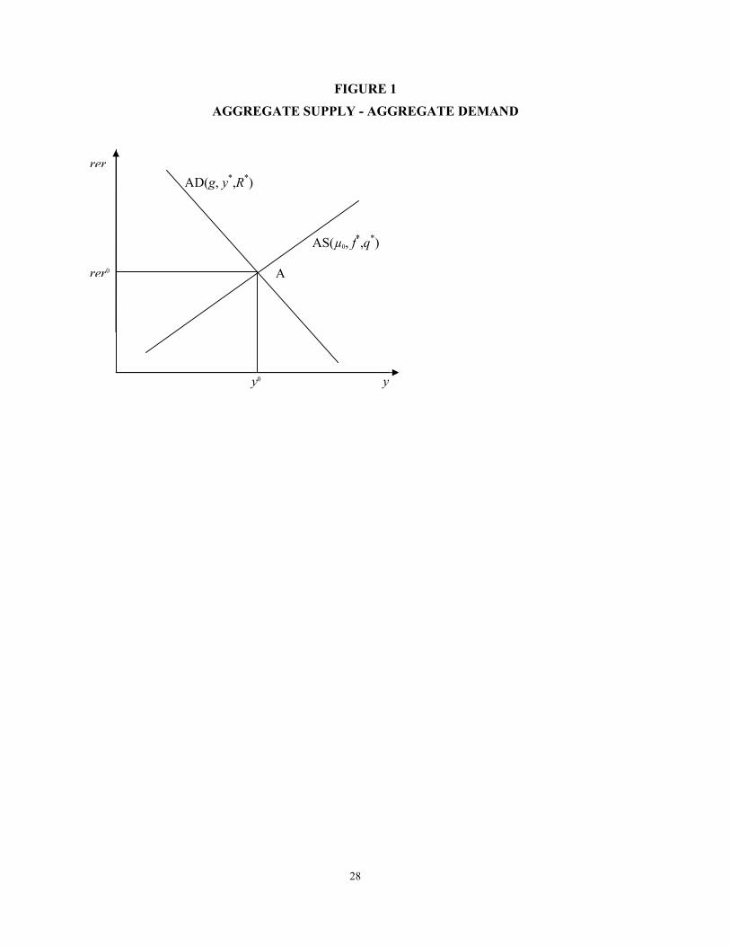
A diagrammatic representation of the solution (10) and (11) is useful. Equations (6)

and (7) are depicted in Figure 1, as aggregate supply (AS) and aggregate demand (AD)

respectively. The solution is at point A, with 0yy = , 0rerrer = .

Due to labour and product market non-competitive behaviour, output in A is less than

it would be under perfect competition, obtained when 0=φ in equation (2), and hh =

(instead of equation (3)).

The position of AD depends on g , ∗y , and *R , while the position of AS depends on

*

0 , fµ and *q . It is straightforward to show that equilibrium output increases with an

increase in government expenditure g , foreign output ∗y , and the international price of the

foreign final good, *f . Also, equilibrium output increases with a reduction in the

international oil price, *q , and the world interest rate, *R . Finally, it increases with a

reduction in 0µ : that is, with a reduction of the mark-up coefficient, φ , a reduction in the

wage pressure parameter, ζ , an increase in the efficiency factor, t , and an increase in the

exogenous labour supply, h . Shifts in aggregate demand parameters move equilibrium output

and the real exchange rate in the same direction, while shifts in aggregate supply parameters

move equilibrium output and the real exchange rate in opposite directions. The government

expenditure multiplier is positive while benign supply side changes (such as a reduction in

the wage pressure parameter and a reduction in the mark-up coefficient) have a positive effect

on output.

Domestic monetary factors play no role in the determination of domestic output and

the real exchange rate. In the classical Mundell – Fleming model with perfect capital

mobility, monetary policy is effective under floating exchange rates because of domestic

nominal price and wage stickiness, which implies that a depreciation of the nominal exchange

rate (as a result of monetary expansion) increases competitiveness and, thus, aggregate

demand and output. In the present model the price of domestic output is not sticky but

14

flexible (although the product market is not fully competitive, that is, 0>φ ). Also, there is

complete wage indexation to the consumer price index. For simplicity, we have called this

‘real consumer wage rigidity’ although this does not mean a fixed real consumer wage: even

under complete wage indexation ( 1=ε ), the real consumer wage (that is, the nominal wage

rate deflated by the CPI) is not fixed, since it depends on labour market conditions ( hh − )

and labour productivity )( hy − – see equation (3). Only under the additional (to 1=ε )

assumption ,0== vn the real consumer wage is fixed and equal to ζ (see Appendix A for an

analysis of this, as well as the “wage militancy” case, defined as 1=ε , ,0=n 1=v ).

Furthermore, the real producer wage (that is, the wage rate deflated by the price of domestic

output, )p is not fixed, which allows for a supply curve which is a positive function of the

real exchange rate. This, combined with non-competitive behaviour in labour and product

markets, makes fiscal policy effective under both exchange rate regimes. In the classical

Mundell – Fleming model, fiscal policy is not effective under a floating exchange rate

because output is fully determined by the LM equation, due to domestic nominal price

stickiness: if pm, and *R are given exogenously, y is fully determined by equation (8).

Buiter (op. cit.) criticizes the traditional literature on optimal currency areas for failing to

distinguish between nominal and real wage rigidity.

The model is capable of handling other exchange rate regimes as well. For instance, if

monetary authorities choose the nominal exchange rate in such a way as to satisfy a target

real exchange rate ( )rerrer = , it can be shown that in general, equilibrium in the model will

be achieved through quantity rationing, since output supply will differ from output demand

for all real exchange rate targets other than 0rer in Figure 1. Under the assumption of a real

exchange rate target, the relevant demand and supply curves in Figure 1 will be the segments

to the left of point A in the diagram.

(ii) Incomplete consumer wage indexation (nominal wage rigidity)

Many models in the literature usually assume an extreme form of nominal wage

rigidity equivalent to 0=ε in our equation (3). Here, we will identify nominal wage rigidity

with incomplete consumer wage indexation, which may be due to incomes policy, the tax

system or the nature of wage contracts.

Under incomplete consumer wage indexation (that is, 10 <≤ ε in equation (3)), we have

10 32 <+< µµ in equation (6); see Proposition 1. Defining ξµµ =−+ 132

15

( 01 <<− ξ ) we can write the supply equation (6) as

*

2

*

210 )( fqeyrer µξµξµµ −++++= (17)

Now, the real exchange rate depends, inter alia, on the nominal exchange rate, and the model

does not exhibit a dichotomy between the real and the monetary sides as before.

Diagrammatically, the position of the aggregate supply curve in Figure 1 now

depends on ,0µ *q , *f

and e and shifts to the right with a nominal depreciation (an increase

in e ), resulting in higher equilibrium output and a lower equilibrium real exchange rate.

The economy can now be described by the system of equations (17), (7), (8), and (9).

(A) Under a floating exchange rate, the endogenous variables are y, rer , e , and p ,

while money, m is exogenous: mm = . Solving the system with respect to output we obtain:

])1()()1([1

1 **2

*20

*

1

0 ymfqRgay ξθγξγµγµγµγξδβξβξηξγξγµ

++−+−−++−+−++

= (18)

An increase in money supply, m , has a positive effect on output, y , since 0<ξ in (18). The

transmission mechanism is the following: An increase in m causes a depreciation of the

nominal exchange rate (see equations (12) and (13) or equation (14)), which, in turn, reduces

the real exchange rate (see (17)) and increases output (see (7)).

An interesting result is that the government expenditure multiplier (dg

dy) is higher

under real consumer wage rigidity than under incomplete wage indexation. Indeed, from (10)

and (18) we can take the difference, ∆ , between the two fiscal multipliers:

)1)(1(1

)1(

1 11

1

11 ηξγγµξγµξγαµαηξγ

ηξγγµξξα

γµ −+++

−−=

−+++

−+

=∆a

>0 (19)

The explanation of this result is the following: An increase in government expenditure, g ,

causes an appreciation of the nominal exchange rate since it increases output and thus, money

demand; see equation (14). Under complete wage indexation, we have seen that a nominal

appreciation of the exchange rate does not affect the real exchange rate. However, under

incomplete wage indexation, it does; see equation (17); In terms of Figure 1, it shifts the AS

curve up, since its position now depends on e as well, resulting in lower output and a higher

real exchange rate.

16

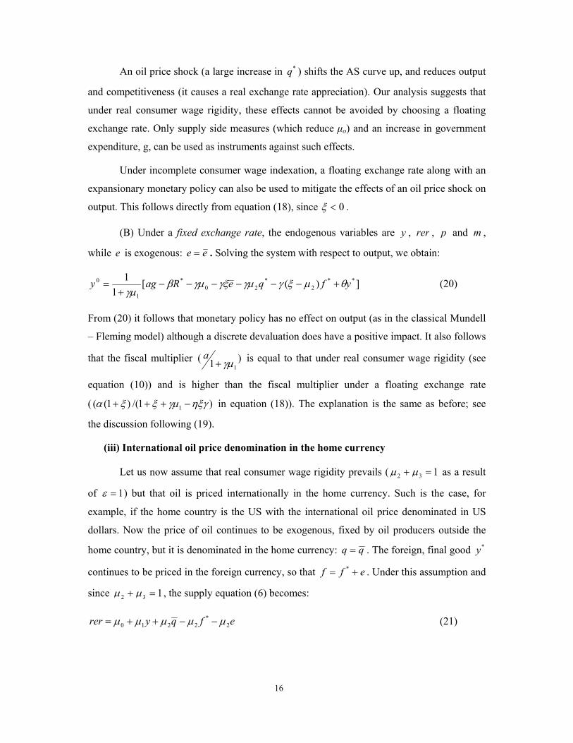
An oil price shock (a large increase in *q ) shifts the AS curve up, and reduces output

and competitiveness (it causes a real exchange rate appreciation). Our analysis suggests that

under real consumer wage rigidity, these effects cannot be avoided by choosing a floating

exchange rate. Only supply side measures (which reduce µο) and an increase in government

expenditure, g, can be used as instruments against such effects.

Under incomplete consumer wage indexation, a floating exchange rate along with an

expansionary monetary policy can also be used to mitigate the effects of an oil price shock on

output. This follows directly from equation (18), since 0<ξ .

(B) Under a fixed exchange rate, the endogenous variables are y , rer , p and m ,

while e is exogenous: ee = . Solving the system with respect to output, we obtain:

])([1

1 **

2

*

20

*

1

0 yfqeRagy θµξγγµγξγµβγµ

+−−−−−−+

= (20)

From (20) it follows that monetary policy has no effect on output (as in the classical Mundell

– Fleming model) although a discrete devaluation does have a positive impact. It also follows

that the fiscal multiplier )1

(1γµ+

a is equal to that under real consumer wage rigidity (see

equation (10)) and is higher than the fiscal multiplier under a floating exchange rate

( )1/()1(( 1 ηξγγµξξα −+++ in equation (18)). The explanation is the same as before; see

the discussion following (19).

(iii) International oil price denomination in the home currency

Let us now assume that real consumer wage rigidity prevails ( 132 =+ µµ as a result

of 1=ε ) but that oil is priced internationally in the home currency. Such is the case, for

example, if the home country is the US with the international oil price denominated in US

dollars. Now the price of oil continues to be exogenous, fixed by oil producers outside the

home country, but it is denominated in the home currency: qq = . The foreign, final good *y

continues to be priced in the foreign currency, so that eff += * . Under this assumption and

since 132 =+ µµ , the supply equation (6) becomes:

efqyrer 2

*

2210 µµµµµ −−++= (21)

17

Equation (21) is qualitatively similar to (17), despite the fact that real consumer wage rigidity

prevails. The real exchange rate depends, inter alia, on the nominal exchange rate as before.

The economy can be described by equations (21), (7), (8) and (9).

(A) Under a floating exchange rate, the money supply is exogenous ( mm = ) and the

endogenous variables are y, rer , p and e. Solving the system with respect to output we

obtain:

yo=

2121

1

ηγµγµµ ++−[αgµ3 – R

*(βµ3 + δγµ2) – γµο - γµ2 q + γµ2f

* + γµ2m + θµ3y

*] (22)

which is qualitatively similar to equation (18). An expansionary monetary policy has a

positive effect on output through a depreciation of the nominal exchange rate. In this case, the

negative effects of a higher oil price on output can be mitigated by supply side measures

(which reduce 0µ ), higher government expenditure, g , and by an expansionary monetary

policy.

(B) Under a fixed exchange rate ( ee = ), money is endogenous, and the solution of

the system of equations (21), (7), (8) and (9) with respect to output gives:

][1

12

**

220

*

1

0 eyfqRagy γµθγµγµγµβγµ

+++−−−+

= (23)

Comparing the fiscal multipliers under fixed and floating exchange rates (from equations (23)

and (22)) we can easily show that fiscal policy is stronger under a fixed rather than a floating

exchange rate. The explanation is the same as before.

Before we proceed to an analysis with two countries, we should stress the basic result

of this section. That is, fixing the international price of imported raw materials in the home

currency introduces an element of nominal rigidity that makes monetary policy effective even

if real consumer wage rigidity prevails. This is not surprising: With nominal wage rigidity, a

nominal depreciation of the home currency shifts the aggregate supply curve to the right,

reducing the real exchange rate and increasing output. In simpler models where the “law of

one price” holds, a nominal depreciation simply reduces the real product wage and increases

output. Similarly, if raw material prices are fixed in the home currency, a depreciation of the

home currency shifts the aggregate supply curve to the right by reducing the real cost of

imported raw materials (see equation (21), the term )(2 eq −µ ) and increases output. An

interesting question, which, however, is outside the scope of the present paper, has to do with

18

the factors which determine the choice of invoice currency for raw materials, as well as the

pricing policies of their producers. A price equation for raw materials, such as oil, can, in

principle, be introduced in the present model, in tandem with the wage equation (3), with

parameters encompassing market structure, exhaustibility considerations, indexation etc.

However it should be kept in mind that the behaviour of the oil price is different from the

behaviour of other raw material prices, mainly due to different market structures. An

empirical issue is the behaviour of real, raw material and commodity prices over a number of

years and their contribution to the behaviour of output and prices in the US and the other

OECD countries. Recent developments in the oil market have revived an interest in

explaining such factors.

3. Two countries: Two large open economies

In the previous section the economy under consideration was small, facing a given

world interest rate, *R , a given price of the foreign, final good, *f , a given foreign output,

*y etc. Now, we will assume that there are two large countries, Country 1 and Country 2

specializing in the production of two final goods 1y and 2y respectively, which are imperfect

substitutes and consumed in both countries. The two goods, 1y and 2y are produced by two

specializing representative producers, one in Country 1 and the other in Country 2. There will

be no strategic interaction between the representative producers of 1y and 2y . They both set

the price of their products in their own markets, treating the other’s output and price as

exogenous. Production inputs are labour and oil. Labour is not mobile between the two

countries and oil is imported in both countries from an outside oil producing zone. The oil

price continues to be exogenous in both countries, but now it is assumed that it is fixed by oil

exporters in the currency of Country 2. This is the only asymmetry characterizing the two

economies. (It might be helpful in this respect to think of Country 2 as the US and Country 1

as the Eurozone). The two countries are characterized by real, consumer wage rigidity, they

are exactly similar in the structure of their product, labour and money markets, and operate

under a floating exchange rate.

The model treats the economy of the “third” country, that is the oil producing “zone”

as exogenous. This prevents the examination of the interaction between oil revenue, the

world interest rate and the exchange rate.

19

Due to perfect symmetry, the product, labour and money markets are characterized by

exactly the same parameters. The same parameters also characterize the output demand

equations (IS equations) in both countries. The assumption of similar parameters in the two

countries is not necessary for the analysis. It is imposed in order to simplify calculations and

is justified since our purpose is to show the effects of oil price denomination in the currency

of one of the two countries.

The two economies are now characterized by the following seven equations:

*

2

*

2110 fqyrer µµµµ −++= (24)

)(2*

2210 epqyrer −−++=− µµµµ (25)

2

*

11 yrerRagy θγβ +−−= (26)

1

*

22 yrerRagy θγβ ++−= (27)

*

11 Rypm δη −=− (28)

*

2

*

2 Ryfm δη −=− (29)

efprer −−= * (30)

The seven endogenous variables are rer , 1y , 2y , e , p , *f , *R . The exogenous variables are

,0µ ,1g ,2g ,1m ,2m q*, with a star denoting prices in Country 2 currency. The exchange rate

e is defined as units of Country 1 currency per unit of Country 2 currency. All variables are

in logs except the interest rate, *R .

Equation (24) is exactly the same as equation (6), that is the real exchange rate

equation of Country 1, with 132 =+ µµ , i.e. with real, consumer wage rigidity. Recall that

equation (6) is derived directly from the inverse supply function (5). Also,

effeqq +=+= ** , .

Equation (25) is the same as (24) for Country 2. It is derived from a similar, inverse

supply function as (5):

*

3

*

2210

* pqyf µµµµ +++= (31)

where epp −=* ; *p is the price of the final good which is produced in Country 1,

expressed in Country 2 currency. It might be useful to think of 1y as production of a “made

20

in the Eurozone” car and 2y as production of a “made in the US” car; p is the euro price of y1

and p* is the dollar price of 1y ; similarly, *f is the dollar price of 2y and f is the euro price

of 2y . The law of one price holds for the same cars, but the prices of the two cars generally

differ because they are imperfect substitutes: eppeff +=+= ** , , but pf ≠ .

Assuming now real, consumer wage rigidity for Country 2 as well ( 132 =+ µµ ) and

subtracting *p from both sides of equation (31), we derive equation (25), that is the real

exchange rate equation for Country 2. Obviously, the (log of the) real exchange rate of

Country 1 is exactly the opposite of (the log of) the real exchange rate of Country 2: when

Country 1’s competitiveness improves, Country 2’s competitiveness worsens by the same

amount.

The meaning of equations (26) – (30) is obvious from the previous section and we do

not need to elaborate on them further. The parameters of the IS - LM equations are the same

in both countries due to the assumed symmetry. In equations (26) and (27) it has been

assumed for simplicity that government expenditure in Country 1 consists only of Country 1

output; likewise for Country 2. Imposing the (reasonable) stability constraints ,1<θ

]2/)2)(1[(1 21 γµθµ −++< , and solving the above system of equations we obtain:

Mggmme )()( 2121 −−−= (32)

rer =γµθ

αµ2)2)(1(

)(

2

211

+−+

− gg (33)

Ν

ΜAg

ΜAg

mq

R

)(2

)(22

1

2

1

0

1

2

1

22

1

21

*µµ

µµ

µ

µ

µ

µ

µ

µ++−+−+

=

∗

(34)

*211

1]

11

1[

2]

1

1

1[

2R

ggy

θβ

θθα

θθα

−−

+Θ

−−

+−

++Θ

= (35)

*122

1]

11

1[

2]

11

1[

2R

ggy

θβ

θθα

θθα

−−

+Θ

−−

+−Θ

+−

= (36)

)1(2

)(

)1(2

)()

1( 2121*

1 θαη

θαη

θηβ

δ+

Θ−−

−

+−

−++=

ggggRmp (37)

21

−−

++= )1

(*2

*

θηβ

δRmf )1(2

)(

)1(2

)( 2121

θαη

θαη

+

Θ−+

−

+ gggg , (38)

where:

0)1

(1 1

2 >−

++−

=θ

ηβδ

µµ

θβ

Ν (39)

02)2)(1(

)2(

2

21 >+−+

−+=

γµθµηµ

M (40)

12)2)(1(

)1(2)2)(1(0

2

12 <+−+

−+−+=Θ<

γµθµγµθ

(41)

0)1(

1 1

2 >−

+−

=Αθ

αηµµ

θα

(42)

Also, from equations (35) and (36) we obtain:

θ+Θ−

=−1

)( 2121

ggayy (43)

θβ

θ −−

−

+=+

1

2

1

)( *

2121

Rggayy , (44)

where equation (43) is the log of the ratio of Country 1 output to Country 2 output. Equation

(44) does not have a direct economic meaning. (It is not the log of world output – see

Appendix B). However it will be used later to calculate the impact on world output of an

equi-proportional increase in government expenditure in both countries (d =1g d =2g d g ).

From equations (32) – (44) we can derive a number of results:

From (32), an increase in the money supply in Country 1 relative to Country 2 leads

to a nominal depreciation (appreciation) of Country 1’s (2’s) currency. An increase in

government expenditure in Country 1 relative to Country 2 leads to a nominal appreciation

(depreciation) of Country 1’s (2’s) currency. If d =1m d 2m and d =1g d 2g there is no change

in the exchange rate.

From (33) and (43) an increase in government expenditure in Country 1 relative to

Country 2 leads to higher output of y1 relative to y2 and a higher real exchange rate for

Country 1. If d =1g d 2g , there is no change in relative output and the real exchange rate. The

22

result that relative output and the real exchange rate depend only on relative government

expenditure is due to the assumption of similar structures in the two economies.

From (34), adverse supply-side changes (such as an increase in the oil price q*), or in

the labour and product market parameters which increase 0µ (see Proposition 2 in section 1),

lead to a higher interest rate, *R , and lower output (see (35) and (36)). A monetary expansion

in Country 2 is a “locomotive” policy: it reduces *R (∂ /*R ∂ 2m = - /2µ 1µN ) and increases

both 1y and 2y (∂ /1y ∂ 2m = ∂ /2y ∂ 2m = )/))(1/(( 12 µµθβ Ν− . Not surprisingly, a

monetary expansion in Country 1, which is characterized by real rigidity, has no effect on the

interest rate or in output (∂ *R /∂ 1m = ∂ /1y ∂ 1m = ∂ /2y ∂ 1m = 0).

From (34), (35), and (36), the effect of higher government expenditure on output is

mitigated by a higher interest rate, due to higher money demand. From (44), assuming

d =1g d 2g = d g and taking into account (34), it is straightforward to show:

0])1()(

)1([

1

1][

1

1)(

2

1

221

221 >−++

−−

=ΝΑ

−−

=+

δθµηµµβδθαµ

θβα

θdg

yyd (45)

It can be shown (see Appendix B) that the left-hand-side of equation (45) is the impact on

world output of an equiproportional increase in government expenditure in both countries

(d =1g d 2g = dg) under the assumption that, initially, the share of each country in world

output is equal to one half. Hence we can interpret equation (45) as saying that the “direct”

effect of an increase in “world government expenditure” on “world output” )1/( θα − ) is

larger than the (negative) interest rate effect ))1/(( Ν−Α θβ , so that the global fiscal

multiplier is positive.

From equations (35) and (36) we obtain:

)()1(2)1(2)1(2 1

2

1

1

ΝΜ

−−

−−

++Θ

=∂

∂

µµ

θβ

θθ N

Aaa

g

y (46)

)()1(2)1(2)1(2 1

2

2

2

ΝΜ

+−

−−

++Θ

=∂

∂

µµ

θβ

θθ N

Aaa

g

y (47)

)()1(2)1(2)1(2 1

2

2

1

ΝΜ

+−

−+Θ

−−

=∂

∂

µµ

θβ

θθ N

Aaa

g

y (48)

23

)()1(2)1(2)1(2 1

2

1

2

ΝΜ

−−

−+Θ

−−

=∂∂

µµ

θβ

θθ N

Aaa

g

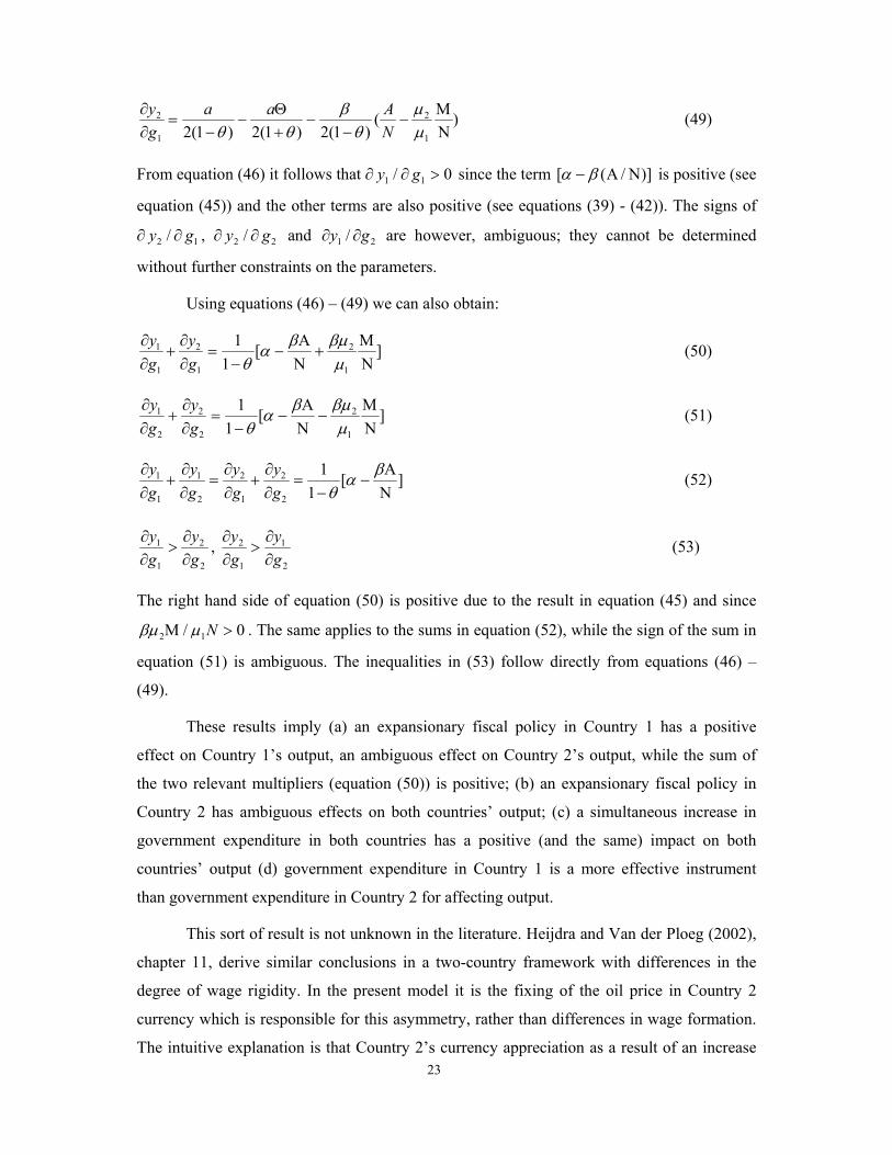
y (49)

From equation (46) it follows that ∂ /1y ∂ 01 >g since the term )]/([ ΝΑ− βα is positive (see

equation (45)) and the other terms are also positive (see equations (39) - (42)). The signs of

∂ /2y ∂ 1g , ∂ /2y ∂ 2g and 21 / gy ∂∂ are however, ambiguous; they cannot be determined

without further constraints on the parameters.

Using equations (46) – (49) we can also obtain:

][1

1

1

2

1

2

1

1

Ν

Μ+

Ν

Α−

−=

∂

∂+

∂

∂

µβµβ

αθg

y

g

y (50)

][1

1

1

2

2

2

2

1

Ν

Μ−

Ν

Α−

−=

∂

∂+

∂

∂

µβµβ

αθg

y

g

y (51)

][1

1

2

2

1

2

2

1

1

1

Ν

Α−

−=

∂

∂+

∂

∂=

∂

∂+

∂

∂ βα

θg

y

g

y

g

y

g

y (52)

2

2

1

1

g

y

g

y

∂∂

>∂∂

, 2

1

1

2

g

y

g

y

∂∂

>∂∂

(53)

The right hand side of equation (50) is positive due to the result in equation (45) and since

0/ 12 >Μ Nµβµ . The same applies to the sums in equation (52), while the sign of the sum in

equation (51) is ambiguous. The inequalities in (53) follow directly from equations (46) –

(49).

These results imply (a) an expansionary fiscal policy in Country 1 has a positive

effect on Country 1’s output, an ambiguous effect on Country 2’s output, while the sum of

the two relevant multipliers (equation (50)) is positive; (b) an expansionary fiscal policy in

Country 2 has ambiguous effects on both countries’ output; (c) a simultaneous increase in

government expenditure in both countries has a positive (and the same) impact on both

countries’ output (d) government expenditure in Country 1 is a more effective instrument

than government expenditure in Country 2 for affecting output.

This sort of result is not unknown in the literature. Heijdra and Van der Ploeg (2002),

chapter 11, derive similar conclusions in a two-country framework with differences in the

degree of wage rigidity. In the present model it is the fixing of the oil price in Country 2

currency which is responsible for this asymmetry, rather than differences in wage formation.

The intuitive explanation is that Country 2’s currency appreciation as a result of an increase

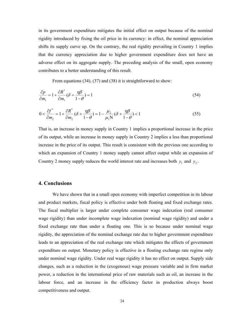
24

in its government expenditure mitigates the initial effect on output because of the nominal

rigidity introduced by fixing the oil price in its currency: in effect, the nominal appreciation

shifts its supply curve up. On the contrary, the real rigidity prevailing in Country 1 implies

that the currency appreciation due to higher government expenditure does not have an

adverse effect on its aggregate supply. The preceding analysis of the small, open economy

contributes to a better understanding of this result.

From equations (34), (37) and (38) it is straightforward to show:

1)1

(11

*

1

=−

+∂∂

+=∂∂

θηβ

δm

R

m

p (54)

1)1

(1)1

(101

2

2

*

2

*

<−

+Ν

−=−

+∂∂

+=∂∂

<θ

ηβδ

µµ

θηβ

δm

R

m

f (55)

That is, an increase in money supply in Country 1 implies a proportional increase in the price

of its output, while an increase in money supply in Country 2 implies a less than proportional

increase in the price of its output. This result is consistent with the previous one according to

which an expansion of Country 1 money supply cannot affect output while an expansion of

Country 2 money supply reduces the world interest rate and increases both 1y and 2y .

4. Conclusions

We have shown that in a small open economy with imperfect competition in its labour

and product markets, fiscal policy is effective under both floating and fixed exchange rates.

The fiscal multiplier is larger under complete consumer wage indexation (real consumer

wage rigidity) than under incomplete wage indexation (nominal wage rigidity) and under a

fixed exchange rate than under a floating one. This is so because under nominal wage

rigidity, the appreciation of the nominal exchange rate due to higher government expenditure

leads to an appreciation of the real exchange rate which mitigates the effects of government

expenditure on output. Monetary policy is effective in a floating exchange rate regime only

under nominal wage rigidity. Under real wage rigidity it has no effect on output. Supply side

changes, such as a reduction in the (exogenous) wage pressure variable and in firm market

power, a reduction in the international price of raw materials such as oil, an increase in the

labour force, and an increase in the efficiency factor in production always boost

competitiveness and output.

25

An interesting result is that fixing the international price of raw materials in the home

currency introduces nominal inertia even under real wage rigidity and makes monetary policy

effective under a floating exchange rate: an increase in money supply entails a currency

depreciation, which reduces the real cost of imported raw materials and boosts output.

In a two, similar country world under a floating exchange rate, real consumer wage

rigidity in both countries, and the price of raw materials fixed in the currency of Country 2,

an expansionary monetary policy in Country 2 is a “locomotive” policy, that is it increases

output in both countries through a reduction in the world interest rate. An increase in money

supply in Country 1 has no effect on output.

An increase in government expenditure in Country 1 has a positive effect on output in

Country 1, an ambiguous effect on output in Country 2, while an increase in government

expenditure in Country 2 produces ambiguous effects on both countries’ output. This is so

because the appreciation of Country 1 currency as a result of higher government expenditure

has no effect on its output due to real wage rigidity (that is, the supply curve does not shift).

In addition, the corresponding depreciation of Country 2’s currency boosts its output due to

nominal inertia (that is, its supply curve shifts to the right). On the contrary, a rise in

government expenditure in Country 2 causes an appreciation of its currency, which due to

nominal rigidity, mitigates the initial positive effect on its output. In addition, the

depreciation of Country 1 currency has no effect on its output due to real rigidity. However, a

simultaneous increase in government expenditure in both countries has a positive impact on

both countries’ output, while the real exchange rate remains unaffected.

One might be tempted to infer that if the Eurozone is characterized by real rigidities

and the US by nominal rigidities (the fixing of international prices of raw materials in US

dollars is one reason, the labour market might be another), the Fed is in a position to affect

domestic and world output but the ECB is not, while Eurozone government expenditure is

more effective as an instrument to affect output than US government expenditure.

26

References

Armington, P. S. (1969), “A theory of demand for products distinguished by place of

production”, IMF Staff Papers, 16, 159-178.

Blanchard, O. and L. Katz (1999), “Wage dynamics: reconciling theory and evidence”,

American Economic Review, 89 (2), 69-74.

Blanchflower, D. and A. Oswald (1994), The wage curve, MIT Press.

Branson, W. and J. Rotemberg (1980), “International adjustment with wage rigidity”,

European Economic Review, 13, 309-332.

Buiter, W. (2000), “Optimal currency areas”, Scottish Journal of Political Economy, 47 (2),

213-250.

Buti, M. (2003, editor), Monetary and fiscal policies in EMU, Cambridge University Press.

Carlin, W. and D. Soskice (1990), Macroeconomics and the wage bargain, Oxford

University Press.

De Grauwe, P. (2001), Economics of monetary union, Oxford University Press.

Dixit, A. (1990), Optimization in economic theory, Oxford University Press.

Dornbusch, R. (1980), Open economy macroeconomics, Basic Books, New York.

Edwards, S. (1989), Real exchange rates, devaluation and adjustment, MIT Press.

Friedman, M. (1953), “The case for flexible exchange rates” in Essays in Positive Economics,

University of Chicago Press.

Friedman, B. (2003), “The LM curve: a not-so-fond farewell”, Working Paper 10123,

National Bureau of Economic Research.

Gali, J. (1992), “How well does the IS - LM model fit postwar US data?”, The Quarterly

Journal of Economics, 107 (2), 709-738.

Heijdra, B. and F. Van der Ploeg (2002), Foundations of modern macroeconomics, Oxford

University Press.

Ishiyama, Y. (1975), “The theory of optimum currency areas: A survey”, IMF Staff Papers,

22, 344-383.

Krugman, P. (2000), “How complicated does the model have to be?”, Oxford Review of

Economic Policy, 16 (4), 33-42.

Lane, P. (2001), “The new open economy macroeconomics: a survey”, Journal of

International Economics, 54, 235-266.

MasColell, A., M. Whinston, and J. Green (1995), Microeconomic theory, Oxford University

Press.

Masson, P. and M. P. Taylor (1992), “Common currency areas and currency unions”,

Discussion Paper No. 617, CEPR.

McCallum, B. (1996), International monetary economics, Oxford University Press.

Moschos, D. and Y. Stournaras (1998), “Domestic and foreign price links in an aggregate

supply framework: the case of Greece”, Journal of Development Economics, 56, 141-

157.

Mundell, R. A. (1968), International Economics, Macmillan, New York.

27

Nickell, S. and M. Andrews (1983), “Unions, real wages and employment in Britain 1951-

79”, Oxford Economic Papers, 35, 507-530.

Nickell, S. (1997), “Unemployment and labour market rigidities: Europe versus North

America”, The Journal of Economic Perspectives, 11 (3), 55-74.

Obstfeld, M. and K. Rogoff (1996), Foundations of International Macroeconomics, MIT

Press.

Obstfeld, M. (2001), “International Macroeconomics: Beyond the Mundell-Fleming model”,

Working Paper 8369, National Bureau of Economic Research.

Rankin, N. (1986), “Debt policy under fixed and flexible prices”, Oxford Economic Papers,

38, 481-500.

Rankin, N. (1987), “Disequilibrium and the welfare maximising levels of government

spending, taxation and debt”, The Economic Journal, 97, 65-85.

Vanhoose, D. (2004), “The new open economy macroeconomics: A critical appraisal”, Open

Economies Review, 15, 193-215.

Vines, D. (2003), “John Maynard Keynes 1937-1946: The creation of international

macroeconomics”, The Economic Journal, 113, F338-F361.

Walsh, C. (2003), Monetary theory and policy, MIT Press.

28

FIGURE 1

AGGREGATE SUPPLY - AGGREGATE DEMAND

AD(g, y*,R

*)

A

AS(µ0, f*,q

*)

rer0

y0 y

rer

29

APPENDIX A

We specify the coefficients ,0µ ,1µ ,2µ 3µ of the (inverse) supply function in equation (5)

in the main text.

Substituting equations (3) and (4) in equation (2), we derive equation (5) (all in the

main text) where:

dvn

vnvn

ελλνσλλσ

µ)1()(1

])1)()[(1(])(1[1 −−−+

++−−+−+= (A1)

dn

vnn

ελλνλλλνλ

µ)1()(1

))(1(])(1[2 −−−+

−−+−+= (A2)

dn

d

ελλνλε

µ)1()(1

)1)(1(3 −−−+

−−= (Α3)

dn

vnvnthnvn

ελλνλλσλζλλφ

µ)1()(1

)])(1()(1[)1()1()1(])(1[0 −−−+

−−+−++−−−−+−+= (Α4)

Using the above equations and the assumptions used in the text, it is straightforward to show:

10 2 <≤ µ , ,10 3 ≤< µ 10 µ≤ . (A5)

Two special cases deserve further attention.

(Α) Τhe “wage militancy” case, defined as: complete wage indexation )1( =ε , no

response of the wage rate to labour market conditions ( 0=n ) and unit elasticity of the wage

rate with respect to labour productivity ( 1=v ). In this case, the coefficients of the inverse

supply function become:

,01 =µ ,02 =µ ,13 =µ ),1/()(0 d−+= ζφµ (A6)

and equations (5) and (6) in the text become:

fdp +−+= )1/()( ζφ (A7)

)1/()( drer −+= ζφ (A8)

which imply that the inverse supply curve is “flat”, or that the real exchange is independent

of output, foreign prices, labour supply h , and the efficiency factor t ; it is exclusively

determined by the mark-up coefficient, φ , and the wage pressure parameter ζ . In terms of

30

Figure 1 in the main text, the AS curve is horizontal (parallel to the y axis) cutting the rer

axis at )1/()( d−+ζφ .

(Β) Τhe “fixed real consumer wage” case, defined as ,1=ε 0== vn . In this case,

the coefficients of the inverse supply function are described by (A9) and (A10):

10 2 << µ , 10 3 << µ , 10 µ< (Α9)

d

t

)1(1

)1()1(0 λ

σζλφµ

−−+−−+

= (Α10)

31

APPENDIX B

We show that the left hand side of equation (45), that is dg

yyd )(

2

1 21 + , is the impact on world

output of an equiproportional increase in government expenditure in both countries

d =1g d 2g = d g under the assumption that, initially, the share of each country in world

output is equal to 1/2.

We define world output (in real terms) as:

21)/( YYFPY += (B1)

where capital letters denote initial variables (not their logs). The term in parentheses is the

real exchange rate, RER, of Country 1, 1Y is Country 1’s production, 2Y is Country 2’s

production, P is the price of 1Y and F the price of 2Y , both expressed in Country 1 currency.

In equation (B1), real world output has been expressed in terms of Country 2 production.

Denoting ln =Y y and taking the differential in (B1), we obtain:

21

21

)(

])[(

YYRER

YYRERd

Y

dYdy

++

== (B2)

Assuming 2

1])/[(])/[()( 212211 =+=+ YYRERYYYRERYRER (which is consistent with our

assumption that the two countries are similar), working out the differential in (B2), dividing

all sides in (B2) by d g (= d =1g d 2g ) and using small letters to denote the logs of the

variables as in the main text, we obtain:

dg

yyd

dg

rerdyyd

dg

dy )(

2

1)()(

2

1 2121 +=

++= , (B3)

since 0)(=

dg

rerd following equation (33) in the main text.

32

33

BANK OF GREECE WORKING PAPERS

1. Brissimis, S. N., G. Hondroyiannis, P.A.V.B. Swamy and G. S. Tavlas, “Empirical

Modelling of Money Demand in Periods of Structural Change: The Case of Greece”,

February 2003.

2. Lazaretou, S., “Greek Monetary Economics in Retrospect: The Adventures of the

Drachma”, April 2003.

3. Papazoglou, C. and E. J. Pentecost, “The Dynamic Adjustment of a Transition Economy

in the Early Stages of Transformation”, May 2003.

4. Hall, S. G. and N. G. Zonzilos, “An Indicator Measuring Underlying Economic Activity

in Greece”, August 2003.

5. Brissimis, S. N. and N. S. Magginas, “Changes in Financial Structure and Asset Price

Substitutability: A Test of the Bank Lending Channel”, September 2003.

6. Gibson, H. D. and E. Tsakalotos, “Capital Flows and Speculative Attacks in Prospective

EU Member States”, October 2003.

7. Milionis, A. E., “Modelling Economic Time Series in the Presence of Variance Non-

Stationarity: A Practical Approach”, November 2003.

8. Christodoulopoulos, T. N. and I. Grigoratou, “The Effect of Dynamic Hedging of Options

Positions on Intermediate-Maturity Interest Rates”, December 2003.

9. Kamberoglou, N. C., E. Liapis, G. T. Simigiannis and P. Tzamourani, “Cost Efficiency in

Greek Banking”, January 2004.

10. Brissimis, S. N. and N. S. Magginas, “Forward-Looking Information in VAR Models and

the Price Puzzle”, February 2004.

11. Papaspyrou, T., “EMU Strategies: Lessons From Past Experience in View of EU

Enlargement”, March 2004.

12. Dellas, H. and G. S. Tavlas, "Wage Rigidity and Monetary Union", April 2004.

13. Hondroyiannis, G. and S. Lazaretou, "Inflation Persistence During Periods of Structural

Change: An Assessment Using Greek Data", June 2004.

14. Zonzilos, N., "Econometric Modelling at the Bank of Greece", June 2004.

15. Brissimis, S. N., D. A. Sideris and F. K. Voumvaki, "Testing Long-Run Purchasing

Power Parity under Exchange Rate Targeting", July 2004.

16. Lazaretou, S., "The Drachma, Foreign Creditors and the International Monetary System:

Tales of a Currency During the 19th and the Early 20

th Century", August 2004.

34

17. Hondroyiannis G., S. Lolos and E. Papapetrou, " Financial Markets and Economic

Growth in Greece, 1986-1999", September 2004.

18. Dellas, H. and G. S. Tavlas, "The Global Implications of Regional Exchange Rate

Regimes", October 2004.

19. Sideris, D., "Testing for Long-run PPP in a System Context: Evidence for the US,

Germany and Japan", November 2004.

20. Sideris, D. and N. Zonzilos, "The Greek Model of the European System of Central Banks

Multi-Country Model", February 2005.

21. Kapopoulos, P. and S. Lazaretou, "Does Corporate Ownership Structure Matter for

Economic Growth? A Cross - Country Analysis", March 2005.

22. Brissimis, S. N. and T. S. Kosma, "Market Power Innovative Activity and Exchange

Rate Pass-Through", April 2005.

23. Christodoulopoulos, T. N. and I. Grigoratou, "Measuring Liquidity in the Greek

Government Securities Market", May 2005.

24. Stoubos, G. and I. Tsikripis, "Regional Integration Challenges in South East Europe:

Banking Sector Trends", June 2005.

25. Athanasoglou, P. P., S. N. Brissimis and M. D. Delis, “Bank-Specific, Industry-Specific

and Macroeconomic Determinants of Bank Profitability”, June 2005.