Aggregate Dynamics in an Economy with Optimal

Long-term Financing

Indrajit Mitra∗

October 28, 2014

Abstract

I introduce optimal dynamic contracting between risk-averse investors and firm

insiders into a dynamic general-equilibrium model with heterogeneous firms. The model

features a time-varying cross-sectional distribution of firms in equilibrium, and I propose

a new numerical solution technique to handle the resulting curse of dimensionality.

I show that even with moderate levels of insider ownership, agency frictions have

significant effects on the dynamics of macro-economic quantities and asset prices. First,

the response of risk-premia and key macro-economic quantities depends in a nonlinear

manner on the history of aggregate shocks. Accumulation of small shocks results in

a disproportionately large decline in aggregate quantities and a rise in risk-premia.

Second, inefficiencies resulting from second-best contractual arrangements help amplify

the effect of primitive shocks and make the economy more sensitive to negative than to

positive shocks. Third, exit rates of firms rise during recessions. Fourth, controlling for

current aggregate productivity, firm exit rates contain incremental information about

future output growth.

∗I thank my committee Leonid Kogan, Andrey Malenko, and Jonathan Parker for comments and useful

discussions. I also thank participants at the MIT Finance Lunch Seminar series, especially Hui Chen, Erik

Loualiche, and Amir Yaron.

1 Introduction

What are the aggregate implications of a misalignment of interest between outside investors

and the decision makers within a firm? Does imperfect corporate control have sizeable effects

on asset prices, such as the market price of risk, and on macro-economic quantities such

as aggregate consumption, output, and investment? This paper answers these questions

in a production economy setting with heterogenous firms exposed to both aggregate and

firm-specific risk.

Frictionless models assume decision makers within a firm maximize the present value

of the firm. All positive net present value projects are funded. The choice of financing is

irrelevant in this frictionless setting, and investment decisions are completely determined by

investment opportunities. There is no need for the firm to maintain financial slack. In reality,

financing decisions matter and interact with investment decisions because of the presence of

various frictions. In certain circumstances, such frictions have very large economic effects, as

illustrated by the recent financial crisis.

To study the effect of financial frictions on a firm’s investment decision, one approach is

to fix the financial arrangement (typically single-period debt) between the firm and outside

investors. I do not take this path for two reasons. First, I view financing choice as an

equilibrium outcome of the interaction between investors and firms. The two parties choose

the best possible arrangement to achieve their objectives subject to constraints arising from

an agency problem. This approach helps us learn about how financing frictions impact the

choices of financial contracts between firms and investors, the joint dynamics of aggregate

macro-economic quantities, such as consumption, output and investment, and asset prices

– all of which are jointly determined in equilibrium. The second reason for adopting this

approach is that in reality, firms use various state-contingent forms of financing. Examples

include lines of credit, debt of multiple maturity, convertible debt, and interest rate derivatives.

1

The dynamics that result from firms using state-contingent financing is expected to be very

different from models in which firms solely use debt-financing.

I integrate a dynamic principal agent model within a stochastic growth model with

investment to determine the joint dynamics of investment, output, and consumption together

with financing policies. The dynamics that is generated from the interaction of this friction

with investment opportunities is quite rich. First, the response of risk-premia and key

macro-economic quantities depends non-linearly on the history of aggregate shocks. In my

model, large drops in aggregate quantities and sharp increases in risk premia are the result of

the accumulation of small shocks. This view of rare disasters is potentially useful because it

gives us a better handle on the probability of deep recessions. Second, the amplification of

primitive shocks is asymmetric – the economy displays a higher sensitivity to negative shocks.

Third, both the level and volatility of firm exit rates increase during recessions. Fourth,

firm exit rates provide additional information about future output growth beyond current

aggregate productivity.

A description of the key elements of my model. Individual firms are operated by insiders

who own a fraction of the firm. I view insiders as composed of at least the CEO and top

level management. The firm needs the insider’s expertise to operate the technology. Insiders

need funding from outside investors. Financing covers operational expenses and also provides

compensation to insiders. The insider’s effort increases expected output, but is costly to

provide. As a result, investors have to provide the right incentives to induce effort. The

financial contract provides incentives to insiders in the form of current and future payments,

together with the threat of possible termination to induce high effort. I assume termination

to be inefficient – insiders receive their outside option which I assume to be a constant

normalized to zero, and outside investors recover only a fraction of the installed capital.

Thus, absent incentive issues, both parties would profit from keeping the match alive. The

financing side is standard in the dynamic contracting literature. In partial equilibrium, the

2

financial contracts in my model are related to the models of DeMarzo and Fishman (2007a),

DeMarzo and Fishman (2007b), and Biais, Mariotti, Plantin, and Rochet (2007) with one key

difference. Unlike these papers which consider the investor to be risk-neutral and therefore

set the discount rate used to value cash-flows to a constant, in my setting the discount rate

is stochastic, and determined endogenously in general equilibrium. The production side of

my model is also standard. The particular version I use is from Gomes, Kogan, and Zhang

(2003). It is a stochastic growth model with aggregate investment and adjustment cost of

capital. This latter feature makes prices more volatile than quantities, a feature of the data.

Some intuition for the main results. History-dependence and non-linear aggregate dynamics

arises from the dead-weight loss due to inefficient liquidations and also because a change in

the aggregate state involves a non-linear adjustment of contract policies. The result is that

the cross-sectional distribution of firms changes shape over time, and the shape is informative

about future dynamics of aggregate quantities and risk premia. A sequence of negative

shocks is manifested by a larger mass of firms in the left tail, and this is why exit rates are

informative about the past history of aggregate shocks. All of the history dependence is

endogenously generated by the friction arising from the agency problem.

The reason for amplification of primitive shocks and the behavior of exit rates are related.

During booms productivity is high and expected to persist making it optimal for investors to

lower the probability of termination during booms. However, to keep the threat of termination

alive for incentive purposes, poor past performance leads to contract termination during

recessions. In general equilibrium, there is a feedback effect. A higher exit rate during

recessions makes these contract poor hedges for the investor, depressing the value of new

contracts even more. This lowers investment in recessions increasing consumption risk, which

in turn lowers the value of investing even more. Lower current investment leads to lower

output in future periods, thus propagating the effect of the bad shock. Recessions are

characterized by an increase in consumption volatility, which translates into a higher risk

3

premium for risky assets.

With exits playing an important role, it is important to accurately track the cross-sectional

distribution, especially the left-tail. This poses a challenge. I present a new approach to solve

for the equilibrium of this economy. I reduce the infinite dimensional distribution to five

parameters by projecting it into a mixture of normal distributions. This turns out to produce

sufficiently high level of convergence of the fixed point problem. The current techniques

in the literature rely on either approximating the distribution by the mean (Krusell and

Smith (1998), or by approximating the entire past history by the last few shocks (Chien and

Lustig (2010)). In a model with exits, the mean is not very informative about the shape and

dynamics of the distribution near the default boundary. The second approach is also not

very convenient in my setting because the dynamics is highly persistent, and would require

tracking a prohibitively long sequence of shocks. My solution approach is of independent use

in any model with defaults or exits.

Any model with financial frictions is expected to generically produce amplification and

persistence of primitive shocks. Prior research on the real effects of financial frictions (for

instance the literature following the seminal works of Kiyotaki and Moore (1997) and Bernanke,

Gertler, and Gilchrist (1999)) confirms this intuition. What do we gain by allowing firms and

investors to choose the form of financing? First, firms do use financing which is intrinsically

state-contingent in nature. Lines of credit, debt of multiple maturity, interest rate derivatives

are just a few of the many securities that firms use1. The second benefit of this exercise, is

that we learn if the effects obtained by fixing the form of financing are robust to allowing

firms and investors a much wider financing choice. For instance, with debt financing, insider

equity holders are unable to hedge their exposure to aggregate shocks and forced to absorb all

risk. Allowing firms to hedge aggregate risk with state-contingent contracts could potentially

1Sufi (2009) reports that 85% of firms in his sample obtained a line of credit. This included fully equityfinanced firms which held no debt.

4

soften the impact of the financial frictions.2 Finally, manager-owned, debt-financed firms is

probably a more appropriate description of small, entrepreneurial firms rather than medium

or large public firms which have a large pool of outside investors.

A convenient feature of the financial contract in my model is that the fraction of the firm

equity owned by insiders is a parameter can be set to a value lower than one. In my numerical

analysis, insiders own only 15% of the firm. Finally, a word about manager preferences.

Although I report results for a risk-neutral manager in my benchmark setting, I solved the

model assuming a risk-averse manager with power utility and risk aversion of 0.5 for low

and moderate levels of consumption, and linear utility for high consumption. The financial

contract in that setting, additionally provides insurance to the manager. At such low levels

of risk-aversion, there is not much quantitative difference in the results. I do not report the

results in this paper.3

Literature review

There is a growing literature which attempts to assess the impact of corporate finance frictions

on asset prices. Dow, Gorton, and Krishnamurthy (2005) look at investment and effects on

state prices where the friction is free cash flow problem by manager. Investors force repayment

by employing a costly auditing technology. Apart from the fact that the financial friction is

different, there are three key differences with the economy modeled in this paper. First, in

their setting, equilibrium policies and prices deviate from the frictionless setting only in good

states of the economy. As a consequence, the market price of risk in their setting decreases

with the strength of the friction. In my setting it increases. Second, the assumption of myopic

investors in their model implies that the free cash flow problem lasts for a single period. In

2In a different setting Krishnamurthy (2003) and Tella (2013) show firms are able to perfectly hedgeaggregate shocks using optimal contracts, and the effects of financial frictions such as amplification andpropagation of primitive shocks completely disappear. My setting differs from these two studies because theoptimal contract is unable to perfectly hedge the aggregate shock resulting in possible inefficient termination.

3Results of this exercise are available on request.

5

my model, the impact of the financial friction extends over multiple periods. Third, they

consider a representative firm, whereas in my model, key features of dynamics just as history-

dependence and non-linearity arises from the heterogenous cross-section. Albuquerue and

Wang (2008) also considers an agency problem similar to the setting here. The key difference

is that they consider investment specific shocks rather than productivity shocks considered

here. Moreover, there are no firm exits in their setting. The aggregate effects of imperfect

enforcement has been studied in Cooley, Marimon, and Quadrini (2004). Again, the friction

is different, and unlike my setting, there are no exits in equilibrium. The sharply contrasting

effects of debt financing versus optimal contracts has been shown by Krishnamurthy (2003),

and more recently in Tella (2013). The key difference between these papers and the setting

here is the presence of inefficient termination in equilibrium. This feature leads to policies

which are non-linear in aggregate shocks. This loss of linearity prevents perfect hedging and

gives rise to the non-linear and history dependent dynamics.

The literature which considers the impact of debt contracts as borrowing constraints

is fairly extensive. Starting with the influential work of Bernanke and Gertler (1989) and

Kiyotaki and Moore (1997) (see also Bernanke et al. (1999)) and more recent results by

Brunnermeier and Sannikov (2014) demonstrate how productivity shocks are amplified and

propagated beyond one period. The bulk of this literature considers single period debt

financing. As a result, the default probability is entirely determined by the distribution of

firm-specific shocks which are an exogenous input to these models. A second difference is that

the cross-sectional distribution of firm characteristics (such as leverage) can be aggregated

because policies are linear. This means that cross-sectional heterogeneity plays no role in

these models, and they are effectively results for a representative firm borrowing from a

representative household. An important recent example of a heterogenous firm model with

borrowing constraints is Khan and Thomas (2013). There are no firm liquidations or exits in

this model. Gomes and Schmid (2009) is a recent paper which considers the effect of firms

6

using long-term debt to finance investment. Equity holders issue infinite maturity debt for

its tax advantage and default when equity value is zero. Coupon size is determined when

the firm enters the economy and held fixed. Gomes, Yaron, and Zhang (2006) consider the

impact of a reduced form specification of financing constraints on asset prices.

Financial contracts similar to the one considered here been discussed in a partial equi-

librium framework. The financial friction in my model is a dynamic version of the hidden

effort model of Holmstrom and Tirole (1997). The financial contract is similar to the discrete-

time models of DeMarzo and Fishman (2007a), DeMarzo and Fishman (2007b), and Biais

et al. (2007) (see also DeMarzo and Sannikov (2006), who provides a characterization of the

contract in a continuous time setting.) Clementi and Hopenhayn (2006) considers the effect

of this friction on firm level investment. The friction in these models is that cash flows are

privately observed by the manager (see also the two period model by Gertler (1992)). De-

Marzo, Fishman, He, and Wang (2012) consider the effects of persistent, publicly observable,

productivity shocks on investment in a traditional q-theory model with agency problems.

Hoffmann and Pfeil (2010) consider optimal managerial compensation policies in a setting

where firms experience persistent productivity shocks. In a different setting, Piskorski and

Tchistyi (2010) consider exogenously specified stochastic interest rates to derive the optimal

mortgage contract. The key difference of this paper with these studies is that the discount

rate used to value cash flows from the contract are stochastic and arise as endogenously from

consumption smoothing motives of the risk-averse representative investor. This difference

drives most of our results. Costly termination implies investment is partially irreversible. In

general equilibrium, this feature adds to the variation in consumption growth and thus to the

market price of risk making downturns more severe than booms. I show that the magnitude

of the asymmetry depending strongly on the investor’s risk-aversion.4 In line with the data,

4A general equilibrium analysis as the one presented in this paper differs from the asset-pricing literate oncredit risk which usually assumes an exogenous stochastic discount rate process to price bonds. In contrast,the covariance between defaults and discount rates is endogenously determined in this economy.

7

risk-premium in this economy is counter-cyclical. A second, less important difference, is that

managers in this economy are risk-averse, in contrast to DeMarzo and Fishman (2007a) and

DeMarzo and Fishman (2007b), where they are risk-neutral. The interaction of incentive and

insurance motives has a long literature – Rogerson (1985), Green (1987), and more recently

by Sannikov (2008). Finally, Gromb (1999) and Quadrini (2004) investigate the effect of

renegotiation to avoid inefficient project termination.

This paper relates to two strands of existing literatures. One studies the effect of financial

frictions on real economic dynamics and asset prices. The second studies optimal dynamic

contracting. I contribute to the first literature by making two changes to the standard

assumptions. First, financial contracts arise as an optimal response to a more primitive

friction thereby avoiding the need to assume particular forms of borrowing constraints.

Second, I relax the assumption of full insider ownership and allow the insider to own only

a small fraction of the firm. I contribute to the dynamic contracting literature by relaxing

the assumption of constant discount rate of the investors. I show that even at the partial

equilibrium level, the difference in discount rates of the investor across aggregate states has

interesting implications for the financial contract. Terminations are not necessarily monotonic

in expected output and depend on the volatility of the discount rate across the states. This

generates novel dynamics of risk-premia and aggregate macro-economic quantities, such as

consumption, output, investment, and asset prices. In general equilibrium, the discount rate is

determined endogenously by the representative household’s consumption and savings decision.

This helps us learn about how financing frictions impact the choices of financial contracts

between firms and investors, the joint dynamics of aggregate macro-economic quantities (such

as consumption, output and investment) and asset prices – all of which are jointly determined

in equilibrium.

The rest of this paper is organized as follows. In Section 2, I describe the model. In

Section 3, I describe properties of the solution. Section 4 reports results of a numerical

8

experiment. Section 5 concludes.

2 The Model

In this section I describe a general equilibrium with a continuum of firms who finance

production by entering into long-term contracts with lenders. I begin by describing the

production sector with technology and investment, and then describe firm entry and details

of the financial contract. Finally, I close the model with a description of the household sector.

2.1 The Environment

Production Sector

There is a continuum of ex-ante identical firms operated by a manager who relies on external

financing to operate his technology. The production technology is linear. It produces the

same homogenous good, which can be used both for consumption and investment

y(x, z, k) = (x+ z)k . (1)

The variable k is the firm’s capital/capacity which is installed when the firm begins to operate

and is held fixed for the life of the firm. Each period, the capital requires a maintenance

cost δk. For simplicity, the parameter δ is assumed to be constant across firms. x is an

aggregate shock common to all firms and z is a firm-specific shock. The variable k is the

firm’s capital/capacity which is installed when the firm begins to operate and is held fixed

for the life of the firm. x is a discrete Markov process with transition matrix Γ

Pr(xt+1|xt) = Γ . (2)

In the baseline model, for simplicity, I assume only two aggregate states. The aggregate shock

x takes on two values x = {xG, xB}. The firm-specific shock also takes on two values z+ > z−,

9

and is independently distributed across time and in the cross-section. The probability of a

higher realization depends on the effort exerted by the firm manager

Pr(z+) =

p, if effort = 1

p−∆p, if effort = 0(3)

Conditional on high effort by the manager, z is normalized to have zero mean5. Providing

high effort is costly – shirking (effort= 0) provides the manager with constant private benefit

Bk. Although realizations of both shocks x and z are publicly observable, investors do not

observe the manager’s effort choice and use observations of firm output to give the manager

incentives to provide high effort.

Prospective managers have no initial wealth. Starting a firm6 requires an initial installation

cost ek where e is randomly drawn from a uniform measure H, and is revealed to the manager

at the beginning of the period. I describe the support of H and its justification in more

detail below. The prospective manager is offered a contract by investors which specifies: (a)

payments that he will receive, and (ii) the probability of termination of the contract ζ. Both

of these policies are functions of the history of the individual manager’s output together with

the history of output of all the managers in the economy. I assume that the law of large

numbers holds, so that the total output in any period is determined by the aggregate shock xt.

Contract policies depend on the discount rate that the investor uses to value future cash flows.

In my setting, the representative household’s equilibrium consumption process determines

the discount rate. The possibility of exits makes the household’s future consumption depend

on the entire cross-sectional distribution of firms (not just the mean). The aggregate state,

which I denote by s, is captured by the the aggregate shock x and its entire past history.

The contract assumes two-sided commitment in which both the manager and the investor

agree to abide by the terms of the contract in all possible contingencies, with no possibility

5The mean is absorbed by x.

6I use the terms project and firm interchangeably.

10

of renegotiation. While this is a restrictive assumption, it provides a useful benchmark and

can be thought of as a limiting case where renegotiation is extremely costly. Such may be

the case if the investors consist of a large dispersed pool of individuals.

For simplicity, four additional assumptions are made about the manager: (a) he has

limited liability, (b) he cannot save privately, (c) he has a time-invariant outside option

normalized to zero7, and (d) he values a consumption stream {ct} as∑

t βtect with time

preference parameter much smaller than that of the outside investor βe << βl. As the

following proposition shows, provided the gain in expected output from the manager exerting

high effort is sufficiently large compared to the private benefit B, the optimal contract elicits

high effort.

Proposition 1 If firm specific shocks satisfy ∆p(z+−z−

)>> B, then there exists an optimal

contract in which it is optimal for the manager to exert high effort.

Proof. Same as in Appendix 1, Proposition 13 of Biais, Mariotti, Plantin, and Rochet (2004).

The Investor’s problem and timing

The financial contract between the outside investor and the firm manager serves three

purposes: it provides for initial installation costs, covers maintenance costs (in the event

of low realizations of z), and also provides insurance to the risk-averse manager. Following

Spear and Srivastava (1987) and Green (1987), I use the dynamic programming approach to

solve for the optimal contract. In this recursive formulation, the present discounted value

of the future payments to the manager, which I denote by V , is a sufficient statistic for the

entire past history of firm-specific realizations of z. In the presence of aggregate risk, i.e. time

varying x, the distribution of continuation values promised to existing managers varies over

7This assumption could be relaxed in a richer model where the manager has an outside option of becominga worker. The lower bound of V is then determined by the rental rate of labor. I leave this extension for thefuture.

11

time, and depends on the realized sequence of aggregate shocks. Therefore, in addition to the

current aggregate shock x, the aggregate state of this economy includes the cross-sectional

measure of continuation values of all managers in the economy, which I denote by µ. The

aggregate state s = {x, µ} therefore includes both the current aggregate shock x and the

cross-sectional distribution µ. In addition to depending on V , contracts are conditioned on

the entire aggregate state s – in particular, each contract implicitly depends on the entire

history of aggregate shocks, and also on the history of output of all existing firms through µ.

The assumption of linear technology allows firm capital k to be scaled out. The investor’s

problem is to offer a contract to the manager that maximizes the present discounted value of

future cash flows (scaled by k)

πt(s)Ft(V ; s) = maxζ(s′),d±(s′),V±(s′)

EΓ

[πt+1(s′)

(ζ(s′)

[(1− χ)(1− δ)

]+

(1− ζ(s)

)Ep(− δ + x′ + z± − d±(s′) + Ft+1(V±(s′); s′)

))]V = EΓ

[(1− ζ(s′)

)Ep(d±(s′) + βeV

′

±(s′))], ∀s′

B/∆p ≤(d+(s′) + βeV

′

+(s′))−(d−(s′) + βeV

′

−(s′))] , ∀s′ ,

s′ = {x′, µ′} , x′ = Γx , µ′ = H(x′, µ) ,{ζ, d±(s′), V±(s′)

}∈ [0, 1]× R4

+ . (4)

The choice variables are the termination probability of the manager ζ, the manager’s payments

d±(V, s) and continuation value V±(V, s). Each of these depend on the aggregate state s,

the current continuation value of the manager, and whether z± is realized. The expectation

EΓ[·] is computed assuming the transition probability matrix Γ for aggregate shocks x, while

the expectation Ep[·] is computed assuming that the agent exerts high effort. This means

that z+ is realized with probability p. The assumption of manager’s limited liability implies

V′±(s) ≥ 0. An interpretation of the lower bound of the manager’s continuation value is

that his outside option is normalized to zero. The law of motion of the aggregate state s

12

includes the law of motion of the cross-sectional distribution of manager continuation values

µ. This law of motion, H(x′, µ), depends both on Γ and on contract policies V ′±. In solving

the contracting problem, agents take this law of motion as given. In a rational expectations

equilibrium, the law of motion used by agents is the realized in the aggregate. Likewise,

investors and the manager take the discount rate π(s′) as given. In general equilibrium,

however, the latter is determined by the representative household’s consumption and savings

decisions, and is determined by the household’s marginal utility evaluated at the equilibrium

aggregate consumption level π(s′)/π(s) = βl(C?t+1(s′)/C?

t (s))−γl

, where C? is the equilibrium

aggregate consumption of the household.

Several comments are in order. First, each period, investors receive a (potentially negative)

payment which is firm output net of maintenance expenditure and the manager’s payment d

till the contract is terminated. When the contract is terminated, the investor takes over the

firm and recovers (1−χ)(1− δ)k of the capital installed (0 < χ < 1). Termination is therefore

costly. Second, in valuing contracts and determining optimal policies, the only stochastic

component of cash flows priced by investors are those associated with systematic market-wide

risk factors. We can either view the representative household as holding a well-diversified

portfolio consisting of all the contracts and a risky-free asset in zero net supply, or picture

identical, individual investors each entering into a long-term contract with a single manager.

In the latter case, individual investors act as pass-throughs – they collect payments and

pass them on to the representative household. Since they belong to the same risk-sharing

household, all investors use the same discount rate to value cash flows. Both these pictures

have identical pricing implications: the idiosyncratic component of cash flows of individual

contracts can be completely diversified away, and are therefore not priced. The household’s

aggregate consumption process is the only systematic risk factor used in pricing risky cash

flows.

Timing in this economy is shown in Fig 16. At the beginning of each period, the aggregate

13

shock x is observed. In accordance with the contractual agreement, manager continuation

values (discounted utility of future payments) are adjusted depending on the realized aggregate

state. As will be shown below, the aggregate state depends not only on the realized value of

the aggregate shock x, but also on the cross-sectional distribution of the continuation values

of all managers in the economy. A public lottery for termination of the project is held in

which firms with low continuation values might exit. Maintenance is paid for continuing firms.

Production takes place next, i.e. firms realize z and produce output. Finally, managers are

paid, new contracts are initiated, and the representative household consumes.

The expectation EΓ[·] is computed assuming the transition probability matrix Γ for

aggregate shocks x, while the expectation Ep[·] is computed assuming that the agent exerts

effort e = 1. This means that z+ is realized with probability p. The assumption of manager’s

limited liability d±(s) ≥ 0, together with the form of the manager’s utility function assumed

implies V′±(s) ≥ 0. An interpretation of the lower bound of the manager’s continuation value

is that his outside option is normalized to zero. The law of motion of the aggregate state

s includes the law of motion of the measure over cross-sectional continuation values µ. In

a rational expectations equilibrium, all agents correctly forecast this law of motion H. In

determining optimal policies, investors and the manager take the discount rate π(s′) as given.

In equilibrium, π(s′)/π(s) = βl(Ct+1(s′)/Ct(s)

)−γl.

To summarize, at the beginning of each period, after observing x, the lottery for ter-

mination is held. Conditional on survival, production takes place. The lender chooses the

manager’s payments d±(V, s) and future promised continuation values V′±(V, s), based on

high/low output, and conditioned on the aggregate state s = {x, µ}. Managers who have

their contracts terminated, have future consumption set to zero. They could be thought of as

having exited the economy. Optimal policies of the financial contract, such as the manager’s

compensation and payments made to the lender, depend on the path of realized cash flows.

This means that even though firms are ex-ante identical, there is ex-post cross-sectional

14

heterogeneity.

Firm entry and investment

Aggregate investment takes place through entry of new firms8. Each period, there is a mass

of potential managers with projects ready to enter the economy. To begin production, a

one-time fixed cost ek has to be paid. This random cost is drawn from a uniform measure H,

and is revealed to potential managers at the beginning of each period. To ensure balanced

growth, I assume the mass of potential entrants is proportional to the measure of existing

firms: H = hNt, where Nt =∫dµt is the total number of firms in existence at the beginning

of period t before any entry and exit in that period. The constant of proportionality h is a

measure of the investment opportunity set. At the aggregate level, this entry cost mimics

adjustment costs and has the effect of making asset prices more volatile.

A new firm is born if the manager is able to secure financing for the project by entering

into a long-term financial contract with an outside investor. I assume perfectly competitive

lending markets so that investors break even. Managers have all the bargaining power and

choose the highest possible payoff subject to the investor’s participation constraint

V0 = sup{V : F (V ) ≥ ek} . (5)

Panel A of Figure 2 shows an example. The contract pays for the initial installation cost,

and in subsequent periods, conditional on continuation, the investor commits to paying

the maintenance cost δk, and compensates the manager according to his past and present

performance. Production begins from the period subsequent to entry. Projects with high

entry costs are unable to secure funding and expire worthless. Panel B of Figure 2 shows

this graphically.

8I borrow this modeling technique from Gomes et al. (2003)

15

Households

I assume that the economy is populated by a single representative household. Individual

investors are assumed to be members of this single risk-sharing household and therefore, they

all share the same stochastic discount factor. This household derives utility from consumption

of the single good Ct and has standard time-separable power utility

E0

∞∑t=0

βtlC1−γlt

1− γl, (6)

where γl is the household’s risk-aversion, and βl is the time preference parameter. The

household derives income from accumulated wealth, and makes consumption and investment

decisions to maximize expected lifetime utility subject to the budget constraint. By assump-

tion, the household is assumed to be more patient than managers (βe < βl). In addition

to investing in firms through the financial contracts, the household also invests in a single

risk-free asset which is in zero net supply. The household takes the risk-free rate r and the

market price of each of the financial contracts F i as given, and chooses consumption Ct and

the portfolio of risk-free asset and financial contracts to maximize utility Ut subject to the

budget constraint.

2.2 General Equilibrium and Aggregation

The equilibrium concept is a Markov perfect competitive equilibrium. The state space of this

problem includes the cross-sectional distribution of manager continuation values, which is

infinite dimensional. The formal definition of the equilibrium is given below:

Definition 1 Recursive equilibrium – A recursive competitive equilibrium is defined as a set

of functions for (i) contract policies Φ(V, x, µ) = {V±(k, V, x, µ), d±(k, V, x, µ), ζ(k, V, x, µ)},

(ii) initial contract state V0(x, µ), (iii) consumption policies of the representative household

C(x, µ), and (iv) law of motion of states s′ ∼ {x′, µ′}, such that (i) individual contracts are

16

optimal, (ii) the initial state is such that the lender breaks even (Eq. 5), (iii) the representative

household’s policies are optimal (Eq. 4)

(iv) the goods market clears

C?(s) =

∫ [xzk − d(s)

]dµ− I(s)− L(s) . (7)

where aggregate investment I and loss from default L are given by

I(s) =

∫ e(s)

0

ekdH +

∫δkdµ−D(s)k =

[h

2e2(s) + δ −D(s)

]k

∫dµ , (8)

L(s) = χ(1− δ)kD(s)

∫dµ . (9)

D(s) is the rate of termination of contracts,

(v) the market for contracts clears

W ?ct =

∫Ft(V )dµt (10)

where W ?ct is the household’s wealth invested in financial contracts, (vi) the bond market clears

W ?bt = 0 (11)

where W ?bt is the household’s wealth invested in the risk-free asset, and (vi) the law of motion

of the cross-sectional distribution of continuation values, H(x′, µ) is consistent with individual

contract policies and the stochastic process for z.

The following proposition summarizes properties of asset returns and the risk-free rate in

the economy.

Proposition 2 The equilibrium stochastic discount factor in this economy is defined by

π′t+1/πt = βl

(C?

t+1

C?t

)−γl, where C?

t is the equilibrium consumption of the representative house-

hold. All gross returns Ri in this economy, satisfy the no-arbitrage relation Et

[πt+1

πtRit+1

]= 1.

17

The risk-free rate, in particular is given by 1 + rt = 1/Et

[πt+1

πt

].

Proof. See Appendix.9

3 Model Solution

I first describe the competitive equilibrium with no moral hazard. In the presence of

moral hazard, aggregate consumption growth depends on the cross-sectional distribution

of continuation values of all managers in the economy. Manager payment policies change

non-linearly when the aggregate state changes, and as a consequence, the cross-sectional

distribution moves over time. The situation is similar to models with aggregate risk, where

non-linearity of policies makes it impossible for the heterogenous cross-section to be aggregated

in a tractable manner (for example Krusell and Smith (1998)). Since the cross-sectional

distribution is infinite dimensional, it is infeasible to solve for prices and policies exactly,

and an approximation approach is necessary to proxy the cross-sectional distribution. The

presence of exits complicates matters, since the mass of managers with low values of V and

close to the default boundary have to be tracked accurately to be able to reliably compute exit

rates. I approximate the cross-sectional distribution by a mixture of two normal distributions

(see Appendix for the computational algorithm). The aggregate state s is approximated by

four numbers: (x, η, µ1, µ2), where the last three parameters are defined on a discrete grid.10

This approach is of independent use in any model of default where it is crucial to track the

shape of the distribution near the left-tail.

9For the contract i, the return Ri =(τ it+1 + F i

t+1

)/F i

t , where F i is the value of the contract aftermaintenance cost and manager payments have been made, i.e. the ex-dividend price.

10As a robustness check I included the variances of the normal distributions as state variables, but theadded computation cost did not produce significant improvements in convergence of the fixed point problem.

18

3.1 No agency problem

When the manager receives no benefit from shirking (B = 0), the agency problem disappears.

All positive NPV projects are funded. By assumption, the manager is sufficiently impatient

so that he values the firm less than outside investors. Managers with positive NPV projects

immediately sell all of firm equity to outside investors. Investors pay for the initial set-up

cost ek and, thereafter, pay per-period maintenance cost δk and receive all cash future flows.

Proposition 3 (Equilibrium allocations) The competitive equilibrium is characterized by

aggregate consumption Ct(x) = ct(xt)∫dµt where

∫dµt is the total number of firms in the

economy. Aggregate output Yt(x) = xt∫dµt, and investment It(xt) =

[h2e2(xt) + δ

]k∫dµt

where

e(xt) = c(xt)γlf(xt) , c(xt) = xt − he2(xt)− δ , (12)

and where f(xi) is

f(xi) = E0

[ ∞∑s=1

βs(c(xs)

s∏j=1

(1 + he(xj)

))−γlxs|x0

].

The manager is assumed to be sufficiently impatient so that βe satisfies both of the following

conditions

e1 ≥ E0

[ ∞∑t

βtext|x0

]=

βex2ζ1 + x1

(1− βe(1− ζ2)

)(1− βe)

(1− βe(1− ζ1 − ζ2)

)e2 ≥ E0

[ ∞∑t

βtext|x0

]=

βex1ζ2 + x2

(1− βe(1− ζ1)

)(1− βe)

(1− βe(1− ζ1 − ζ2)

) .Proof. See Appendix.

With no moral hazard, there are no exits and as seen from Proposition 3, the current

aggregate state x and the total number of firms are sufficient statistics for aggregate output,

investment, consumption, and asset prices. Details of the cross-sectional distribution do not

matter for quantities and prices. Primitive shocks do not propagate and there is no history

19

dependence.11

3.2 With moral hazard

With positive private benefit to the manager from shirking, investors need to induce high

effort by providing incentives using the contract described in Section 2.1. Without aggregate

uncertainty xG = xB, the investor’s consumption growth rate is a constant in the steady-state,

and therefore, the investor’s discount rate βl(Ct+1/Ct)−γl is constant. This is the setting

considered in DeMarzo and Fishman (2007a), DeMarzo and Fishman (2007b), and also in

Biais et al. (2007). I quickly review the features of the optimal contract in this simple case.

The reader is referred to these papers for more details.

The form in which incentives are provided depend on the manager’s continuation utility.

Figure 3 shows the investor’s value of future cash flows from the contract as a function of

the manager’s continuation value. It is weakly concave. At very low values, increasing the

manager’s continuation value lowers the probability of inefficient termination of the firm.

This leads to an initial increase in the value (to the investor). At very high continuation value,

increasing the manager’s continuation value leads to a decrease in value to the investor because

it constitutes a wealth transfer from the investor to the manager. Figure 4 shows optimal

policies. The panel on the left shows the manager’s continuation value after realization of firm

output. His continuation value changes from V to V+ for high output (solid, blue curve), and

to V− (dashed, red curve) for low output. The spread provides incentives for him to provide

high effort. At very low levels of manager’s continuation value, this spread cannot be provided,

and incentives are provided by threatening termination. The panel on the right, shows cash

policies of this contract. From the figure, we see that cash is paid only after a sufficiently

high continuation value is achieved by the manager. The solid, blue curve shows payments

11Note that although there is no additional propagation of primitive aggregate shocks, consumption growthis persistent because the aggregate productivity shocks are persistent.

20

received by the manager after a high cash flow realization, while the dashed, red curve shows

his cash compensation for low output. To sum up, for very high continuation values, the

manager is compensated by cash payments. At intermediate values, he is compensated by

future promises. At very low continuation values, incentives are provided through the threat

of terminating the contract. Figure 5 shows the the fractional loss in firm value due to the

borrowing constraints arising from the moral hazard problem. The solid, black curve shows

firm value defined as the sum of the investor’s value and the manager’s continuation utility.

Firm value is lower than the first-best value because of the cost of providing incentives to the

manager and because of the possibility of an inefficient termination lowers the value of the

firm. The dotted, blue curve plots the stationary distribution of manager continuation values.

In this example, about half of the firms suffer a loss greater than 10%.

Are there more inefficient terminations if the manager’s private benefit is higher? From

Eq. 4, incentive compatibility requires an increase in the spread of manager’s continuation

value for higher B. This is intuitive, and means that a stronger moral hazard problem

necessitates a higher level of insider ownership. A higher volatility of continuation values

increases the risk of termination. However, in this case, it is optimal for the investor to

postpone payments even longer and instead increase the manager’s continuation value at a

higher rate away from the termination boundary. To compare the termination rates in the

steady-state, in Figure 6, I plot the stationary distributions corresponding to a high and low

value of B/∆p(z+−z−). The dotted black curve is for a lower value of B/∆p(z+−z−) = 0.20,

while the solid blue curve is for higher B/∆p(z+ − z−) = 0.40. A higher value of B is

characterized by a distribution which is wider (because of higher volatility), but the core of

the distribution is also pushed to higher values of V reflecting the contract’s precautionary

motive to reduce the risk of termination from a more volatile V . The net result of these

opposing forces is that the increase in exit rate is very gradual. 12

12I find the increase to be non-monotonic in B/∆p(z+ − z−), but this could be a numerical artifact.

21

Implementation of the optimal contract is not unique. DeMarzo and Fishman (2007b)

show how to implement this contract using a combination of inside and outside equity, long-

term debt, and a line of credit. In this implementation, the manager keeps B/∆p(z+ − z−)

of firm equity, while outsiders hold the remaining fraction of equity, together with long term

debt with fixed coupon payments, and a line of credit. None of the results presented in this

paper depend on the particular form of implementation. Therefore, I do not discuss this

further, and refer the interested reader instead to DeMarzo and Fishman (2007b) and Biais

et al. (2007).

The discussion above focussed on the contract under no aggregate uncertainty. Next I

discuss dynamics under aggregate uncertainty.

Aggregate Uncertainty

With aggregate shocks, the distribution of continuation values (and therefore manager

payments), changes over time. There is no steady-state distribution to which the economy

settles into, and this gives rise to rich dynamics which depends on the cross-sectional

distribution. For this reason, proving the existence of an equilibrium is difficult. This is not

unique to the set-up here and occurs in problems with incomplete markets which feature

aggregate uncertainty.

As Proposition 4 shows, the introduction of public lotteries makes the investor’s value

function concave in the manager’s continuation utility. The marginal cost of providing

incentives, −F ′(V ) is bounded from above by 1.

Proposition 4 The investor’s value function F is a concave function of the manager’s

promised utility V . The slope is bounded by F ′(V ) ≥ −1.

Proof. See Appendix.

How does the dynamics of risk premia and macro-quantities compare between the fric-

tionless economy and the one with an agency problem? The frictionless economy does not

22

feature exits. Risk premia and growth rates of consumption, output, and investment are

given by the aggregate productivity shock. In the economy with the friction turned on, the

dynamics is a lot more interesting.

In the presence of aggregate productivity shocks, contract policies such as termination,

depend on two forces. I call them the profitability effect and the discount rate effect. These

forces act in opposite directions which is best illustrated by an example. Suppose the aggregate

state changes from xB to xG. By assumption, aggregate shocks are persistent. This means,

that the present value of future cash flows to the investor is now higher than it was before.

Investors will now want to reduce the probability of termination and capture higher profits.

They achieve this by increasing the continuation values of managers, thereby lowering their

risk of termination, should they draw a low firm-specific shock z. However, to keep the threat

of termination real, managers will have their continuation values lowered when the aggregate

state changes from xB to xG. Figure 7 shows this behavior for low V . In fact, managers

with V below a threshold, have their continuation values set to zero, and are immediately

terminated. However, there is another force at play which has to do with the change in the

investor’s discount rate. In the low productivity state, the discount rate of the investor is

higher than in the state xG. In other words, relatively speaking, the manager is more patient.

This makes it cheaper to delay paying the manager in this state, in exchange for higher

payments in the future. This behavior is seen in Figure 7 for high values of V .

In general, whether the profitability effect, or the discount rate effect dominates, depends

on the volatility of the stochastic discount rate of the investor, the aggregate volatility of cash

flows, and the dead-weight loss from terminations. In aggregate states with high volatility

of the stochastic discount rate, the discount rate of the investor is much higher in the bad

state compared to the good state. In this situation, investors will optimally terminate poorly

performing managers in the good aggregate state. This feature of the contract makes it

distinctly different from pure long-term debt where the default rate is always counter-cyclical.

23

Having said that, in the numerical analysis presented in the next section, I choose parameters

which result in counter-cyclical exits.

With this choice of parameters, the dynamics of risk premia is counter-cyclical and

highly non-linear. To fix ideas, suppose the economy starts from the stochastic steady-state.

Realization of a low aggregate shock xB results in manager’s continuation values being

adjusted as shown in Figure 7. Managers with low continuation values are either immediately

terminated, or, have their continuation values adjusted downward. This leads to an increase

in the mass of firms near the default boundary, as shown in Figure 8. The dotted, blue curve

is the stochastic steady-state distribution, and the solid, red curve is the resulting distribution

after realization of xB. If a low aggregate shock is realized in the following period, the exit

rate will increase because there is a higher number of managers close to the termination

boundary. Figure 9 shows the increase in exit rates after two successive realizations of xB.

Risk premium follows a similar pattern. Higher exits in states with high marginal utility of

the representative household lowers the value of investment. As a result, fewer firms enter

the economy. Lower investment raises the consumption risk. This causes the market price of

risk to go up, as shown in Figure 10.

The result of several bad shocks is more severe. With each successive realization of xB,

more firms are pulled closer towards the termination boundary. This causes the exit rate

to increase sharply as shown in Figure 11. A much higher rate of terminations when the

household’s marginal utility is high causes a sharp drop in the value of potential entrants

leading to a big drop in investment. In general equilibrium, this causes consumption to be

very volatile leading to the sharp increase in the market price of risk shown in Figure 12.

The upshot of this is that risk-premia is not only counter-cyclical, but also depend on

the history of realized aggregate shocks. It is important to point out that the behavior is

also not guaranteed to be monotonic in aggregate shocks. With very high discount rate of

24

the household, termination behavior could switch.13 In general, the dynamics of investment,

output, consumption, and asset prices in this economy is a highly non-linear, path-dependent

function of aggregate shocks.

4 Quantitative Results

I summarize results comparing the frictionless model (B = 0) with moderate and high values

of B. The first set of results are for unconditional moments of the aggregate macroeconomic

quantities and asset prices. The purpose is mainly to make sure that the values of parameters

chosen are reasonable and that results are not due to unreasonable parameter choices. Next I

report how aggregate consumption, investment, and output vary over the business cycle. The

model is solved using the approach outlined in the Appendix.

4.1 Parameters

There are 12 parameters in the model. Although the model is calibrated and computed at

quarterly frequency, I annualize all parameters for easy interpretation. The two preference

parameters of the representative investor are βl = 0.998, risk-aversion of γl = 10. The

manager’s time-preference parameter is set to be 0.92. The technology parameters consist of

the transition matrix Γ, with the (annual) transition intensity out of the state x = xG set at

ζG = 0.33, and the transition intensity out of state x = xB is set to ζB = 0.70. Aggregate

shocks x are thus assumed to be persistent. The ratio xG/xB = 1.091 and is chosen to match

the unconditional volatility of output growth. With this choice of xB,G and the transition

matrix, both aggregate states have the same amount of consumption risk and therefore any

time variation in conditional volatility arising from constraints is purely the result of the

friction arising from the agency problem. It might appear though, that with this choice of

transition matrix, recessions and booms are much shorter lived than in the data. However,

13In the current calibration, this probably requires many more realizations of xB .

25

because the drop in aggregate output from xG to xB is relatively small, the model counterpart

of recessions in the data are two or more successive realizations of xB. The firm-specific

shocks z± are chosen to occur with equal probability (p = 0.5), and the size of |z±| is chosen

to correspond to an annual volatility of 40%. The depreciation rate of capital is set to 5%

per year, which corresponds to δ = 0.0125. Finally, the loss from termination of contracts χ

is assumed to be such that the value of the firm after default is 0.6 times the first-best value

of the firm. This amounts to setting χ = 0.35. The entry rate h is chosen so that the annual

growth rate of consumption in the model with financing friction is 1.5%.

The strength of the moral hazard problem depends on B/∆p(z+ − z−) = 0.15. In this

numerical exercies, I set B/∆p(z+ − z−) = 0.15, which corresponds to insiders holding 15%

of the equity of the firm in the steady-state (with no aggregate uncertainty). Jenter and

Lewellen (2013) reports average CEO ownership in public firms is 5.5%. I choose a higher

value because insiders in the model is anyone who has significant influence over decisions

made within a firm. For the frictionless model B = 0. I simulate 1000 independent panels of

N = 105 firms over a time period of 300 quarters. All reported values are averages over these

1000 independent simulations.

4.2 Aggregate Macro and Asset Prices

Unconditional averages

Table 2 show unconditional moments of aggregate macroeconomic quantities and asset

prices. The top panel shows investment, output, consumption, and exits (in this stylized

simple model, termination of contracts correspond to exits). The model produces aggregate

investment levels of 20% of output, which is close to that observed in the data. This is not

a prediction, rather parameters were chosen to hit this target. With the same parameters,

the frictionless model predicts a much higher investment rate, because, without costly exits,

the value of entering is much higher for both realizations of the aggregate shock. The first

26

two moments of the household’s consumption growth process is also close to the empirical

counterparts. The frictionless model features much less consumption risk. The risk of costly

termination during recessions magnifies consumption volatility considerably. Although the

model is able to match the empirical volatility of consumption and output growth, it is

unable to generate sufficient investment volatility. This could be remedied by including

investment specific shocks which increase the availability of good projects during good times

( hG > hB). The frictionless model has an even lower investment volatility. The amplification

in investment volatility with agency frictions arises due to a higher exit rate during recessions

when the household’s marginal utility is high. This lowers the value of entering even more in

the low state (x = xB).

Exits in my model are counter-cyclical. The model is quite stylized and firm exits

correspond to insiders being fired. In the data, these two interpretations are quite different.

The level of CEO terminations reported by Kaplan and Minton (2012) is 15.8% (a previous

version of their paper which used data till 2004 reported a lower value of 12.8%). The model

presented here produces a much lower average termination rate of 2.9%. This is expected,

for CEO’s are also terminated for factors different from agency problems, such as investors

learning about CEO’s skill. The model presented here does not consider such factors for

simplicity. Firm exit rates are also in the same range, although most of the exits are for small

firms which typically have much higher insider-ownership than the value used in my numerical

analysis (15%). In the data, the volatility of the de-trended rate of CEO termination is

about 3.4% which is close to the model prediction of 2.9%. The termination of exits is highly

correlated with output growth: the model prediction is 0.88, while Eisfeldt and Rampini

(2008) report a value of 0.9. Note, that there are no exits in the frictionless model.

The lower panel of Table 2 shows that asset pricing moments are also close to the

empirical counterparts. The equity premium, defined as the expected excess return over the

risk-free rate to a claim on aggregate output is lower than in the data. This is because in my

27

model, I define equity-premium to be the excess return to a claim on aggregate consumption.

In the data, however, the stream of payments priced are dividends, which are much more

volatile than consumption. The high expected return on aggregate consumption is because

of three reasons. First, persistent variations of consumption growth increases the investor’s

precautionary savings motive by lowering both the level and the volatility of the risk-free rate.

Part of this predictability is inherited from the predictability of productivity shocks. However,

successive low realizations of x depletes the number of firms which takes time to rebuild.

With exits, the time to rebuild is even longer, which further depresses the risk-free rate and

increases the equity premium. The second reason is because exits in the bad aggregate state

amplify the volatility of consumption. Finally, a high choice of risk-aversion (γl = 10) also

increases the expected return on risky consumption. Costly termination in states in which

the investor’s marginal utility is high, raises the expected return producing a higher equity

premium and a higher Sharpe ratio.

4.3 Business cycle properties

The presence of financial frictions introduces changes both for aggregate quantities and prices,

and improves the model’s ability to match the data. There are three important and noticeable

changes. First, the asymmetric response of growth rates of output and investment is much

more pronounced (by a factor of 1.35 for the numerical example). Second, the market price of

risk (Sharpe ratio) is time-varying in the economy with borrowing constraints. Third, there

is additional propagation of primitive productivity shocks. I describe each of these in turn,

and provide intuition behind the results.

Asymmetric business cycles

Aggregate investment is pro-cyclical because of increased exits during recessions and lower

levels of entry. Figure 13 shows the asymmetric response of investment to positive and

28

negative shocks. As the solid, blue curve shows, a one-standard deviation positive shock in

the aggregate shock x, produces a 4.1% rise in investment. The lower dotted, red curve shows

that a negative shock of the same magnitude produces a 5.5% drop. Output growth exhibits

a similar asymmetry as seen from Figure 14.

The asymmetric response is due to defaults occurring in states in which the investors’s

marginal utility is very high. With a risk-averse lender, a negative realization of the aggregate

shock, x, has two effects. It lowers current output (by lowering productivity), and secondly,

because the exit rate goes up precisely when marginal utility is high, the value of entering

goes down. This leads to even lower investment. Non-zero risk premia causes investment

(and also output) to respond asymmetrically to positive and negative shocks. This intuition

is confirmed by Figure 15. The figure plots the amount of asymmetry as measured by the

ratio of the magnitude of the drop in investment in response to a negative productivity shock,

to the increase when a positive shock of the same magnitude is realized. As expected, the

asymmetry is larger if the investor is more risk-averse.

Time varying risk premia and predictability

The market price of risk depends on the volatility of aggregate consumption growth. In the

frictionless economy, consumption is completely determined by the current aggregate shock x

and the total number of existing firms. Consumption growth inherits the Markov nature of

the primitive productive shocks. There is no further dependence on past history. The baseline

model is calibrated so that the conditional volatility of consumption growth, and hence the

market price of risk, in the frictionless setting is the same across the two aggregate states

xG,B. For the economy with borrowing constraints, however, the exit rate depends both on

the aggregate shock, and on the shape of the left-tail of the distribution. For instance, the

exit rate is higher when the aggregate state changes from xG to xB if the cross-sectional

distribution of manager continuation values is skewed more to the left. This introduces two

29

changes to the conditional volatility of consumption growth with accompanying pricing effects.

First, consumption growth is more volatile during recessions than in booms because of an

increase in the exit rate during recessions. The second difference from the frictionless setting,

is that consumption volatility depends on the sequence of realized aggregate shocks. When

a low aggregate shock is realized, it is optimal for the contract to reduce the continuation

value of managers with low continuation values. This increases the mass of managers near

the default boundary to increase. Consequently, a second low realization of x will lead to an

even higher number of exits compared to the previous period. This accelerated exit behavior

is shown in Figure 11 together with a similar behavior for the volatility of the stochastic

discount rate in 12.

A prediction of the model therefore, is that controlling for current realized aggregate

productivity, the past history of aggregate shocks is informative about future growth rates of

investment, output, and consumption. Since I approximate the cross-sectional distribution by

a mixture of normals, the relative weight of the normal with lower mean acts an approximate

store of the past history of shocks. For instance, successive realizations of xB lead to an

increase in the relative weight of the normal distribution with lower mean. Table 3 shows that

regression results for output and investment growth after controlling for current aggregate

shock. In line with our intuition, the slope is negative and is significant.

5 Conclusion

In this paper, I provide a simple, unified framework to illustrate the interaction of financing

frictions on key aggregate quantities and risk premia. The presence of financing frictions lead

to rich aggregate dynamics of macro-economic quantities and asset prices, and improves the

predictions of neo-classical frictionless models along several dimensions. A key finding of this

paper is that in the presence of financing friction, the response of the economy to aggregate

shocks is both non-linear and history-dependent. The marginal effect of an aggregate shock

30

depends on the sequence of shocks that preceded it. This findings of this paper also provides

an alternate view of deep recessions. Rather than being the result of a single large shock,

they are the consequence of a series of small negative shocks. This is useful because while

it is much harder to estimate the probability of a single large rare event, the probability of

realization of a long sequence of small shocks which individually occur frequently can be

better estimated.

The essential elements of the dynamics induced by firm heterogeneity in this model

might carry over to other settings. It would be interesting to see if higher moments of the

cross-sectional distribution of firm performance are able to better capture the state of the

economy at a given moment, and hence better predict for aggregate dynamics.

31

References

Albuquerue, R. and N. Wang (2008). Agency conflicts, investment, and asset pricing. Journal

of Finance 63 (1), 1 – 40.

Bernanke, B. and M. Gertler (1989). Agency costs, net worth, and business fluctuations. The

American Economic Review 79 (1), 14 – 31.

Bernanke, B., M. Gertler, and S. Gilchrist (1999). The financial accelerator in a quantitative

business cycle framework. Handbook of Macroeconomics 1 (C), 1341 – 1393.

Biais, B., T. Mariotti, G. Plantin, and J.-C. Rochet (2004). Dynamic security design. Working

paper, CEPR.

Biais, B., T. Mariotti, G. Plantin, and J.-C. Rochet (2007). Dynamic security design:

Convergence to continous time and asset pricing implications. The Review of Economic

Studies 74 (2), 345 – 390.

Brunnermeier, M. and Y. Sannikov (2014). A macroeconomic model with a financial sector.

The American Economic Review 104 (2), 379 – 421.

Campbell, J. (1998). Entry, exit, embodied technology, and business cycles. Review of

Economic Dynamics 1, 371 – 408.

Chien, Y. and H. Lustig (2010). The market price of aggregate risk and the wealth distribution.

Review of Financial Studies 23 (4), 1596 – 1650.

Clementi, G. L. and H. A. Hopenhayn (2006). A theory of financing constraints and firm

dynamics. The Quarterly Journal of Economics 121 (1), 229 – 265.

Cooley, T., R. Marimon, and V. Quadrini (2004). Aggregate consequences of limited contract

enforceability. The Journal of Political Economy 112 (4), 817 – 847.

DeMarzo, P. and M. Fishman (2007a). Agency and optimal investment dynamics. Review of

Financial Studies 20 (1), 151 – 188.

DeMarzo, P. and M. Fishman (2007b). Optimal long-term financial contracting. Review of

Financial Studies 20 (1), 2079 – 2128.

DeMarzo, P. M., M. J. Fishman, Z. He, and N. Wang (2012). Dynamic agency and the q

theory of investment. The Journal of Finance 67 (6), 2295 – 2340.

DeMarzo, P. M. and Y. Sannikov (2006). Optimal security design and dynamic capital

structure in a continuous-time agency model. The Journal of Finance 61 (6), 2681 – 2724.

32

Dow, J., G. Gorton, and A. Krishnamurthy (2005). Equilibrium investment and asset prices

under imperfect corporate control. The American Economic Review 95 (3), 659–681.

Eisfeldt, A. L. and A. A. Rampini (2008). Managerial incentives, capital reallocation, and

the business cycle. The Journal of Financial Economics 87 (1), 177 – 199.

Gertler, M. (1992). Financial capacity and output fluctuations in an economy with multi-

period financial relationships. Review of Economic Studies 59 (3), 455 – 472.

Gomes, J., L. Kogan, and L. Zhang (2003). Equilibrium cross section of returns. Journal of

Political Economy 111 (4), 693 – 732.

Gomes, J., A. Yaron, and L. Zhang (2006). Asset pricing implications of firms financing

constraints. Review of Financial Studies 19 (4), 1321 – 1356.

Gomes, J. F. and L. Schmid (2009). Equilibrium credit spreads and the macroeconomy.

Working paper, Duke and Wharton University.

Green, E. (1987). Lending and the smoothing of uninsurable income. Technical report, E.

Prescott and N. Wallace (eds).

Gromb, D. (1999). Renegotiation in debt contracts. Working paper, M.I.T.

Hoffmann, F. and S. Pfeil (2010). Reward for luck in a dynamic agency model. Review of

Financial Studies 23 (9), 3329 – 3345.

Holmstrom, B. and J. Tirole (1997). Financial intermediation, loanable funds, and the real

sector. Quarterly Journal of Economics 112 (3), 663 – 691.

Jenter, D. and K. Lewellen (2013). Ceo preferences and acquisitions. Working paper.

Kaplan, S. N. and B. A. Minton (2012). Has ceo turnover changed? Working paper.

Khan, A. and J. Thomas (2013). Credit shocks and aggregate fluctuations in an economy

with production heterogeneity. The Journal of Political Economy .

Kiyotaki, N. and J. Moore (1997). Credit cycles. Journal of Political Economy 105 (2), 211 –

248.

Krishnamurthy, A. (2003). Collateral constraints and the amplification mechanism. Journal

of Economic Theory 111 (2), 277 – 292.

Krusell, P. and A. A. Smith (1998). Income and wealth heterogeneity in the macroeconomy.

Journal of Political Economy 106 (5), 867 – 896.

33

Piskorski, T. and A. Tchistyi (2010). Optimal mortgage design. Review of Financial Studies 23,

3098 – 3140.

Quadrini, V. (2004). Investment and liquidation in renegotiation-proof contracts with moral

hazard. Journal of Monetary Economics 51 (4), 713 – 751.

Rogerson, W. P. (1985). Repeated moral hazard. Econometrica 53 (1), 69 – 76.

Sannikov, Y. (2008). A continuous-time version of the principal-agent problem. The Review

of Economic Studies 75 (3), 957 – 984.

Spear, S. and S. Srivastava (1987). On repeated moral hazard with discounting. Review of

Economic Studies 54 (4), 599 – 617.

Sufi, A. (2009). Bank lines of credit in corporate finance: An empirical analysis. The Review

of Financial Studies 22 (2), 1057 – 1088.

Tella, S. D. (2013). Uncertainty shocks and balance sheet recessions. Working paper, M.I.T.

34

Appendix

A Proofs of Propositions

Proof of Proposition 2

The household takes the risk-free rate, rt, and the ex-dividend contract prices F it as given.

The household’s Bellman equation is

Ut(g,~b, s) = maxC≥0,g′,~b′

[u(Ct) + E

[βlUt+1(g′,~b′, s′)

]], s = {x, µ} , (13)

subject to the budget constraint

gt +∑

i∈Continue

bit(F it + yit − dit − δ

)k +

∑i∈Default

(1− χ)(1− δ)k

−∑

i∈Entry

eik =gt+1

1 + rt+

∑i∈Continue

bit+1Fit + Ct (14)

where g and ~b are the household’s holding of risk-free asset and the long-term contracts, and

dit is the payment received by the manager from contract i in period t. The aggregate state s

explicitly depends on aggregate shock x and also on the distribution of continuation values of

surviving managers. The expectation is over realizations of x′ given that the current shock is

x, with exogenously specified transition probability matrix Γ. By “continue” I mean only

those firms which are still in existence. This excludes new entrants. Finally, 1 − χ is the

recovery rate given default has occurred. The law of large numbers is assumed to hold, so

that Ct does not depend on individual realizations of firm-specific shock z.

Market clearing: In equilibrium, the bond market and the market for financial contracts

clear

gt = gt+1 = 0 , bit = bit+1 = 1 , (15)

for continuing firms i. Substituting the market clearing conditions into the budget constraint

Eq.14, prices (rt and F it ) drop out, and the goods market clearing condition becomes

Ct +∑

i∈Continue

dit = Yt − It − Lt ,

35

where

It =∑i∈All

δk +∑

i∈Entrants

eik −∑

i∈Default

k ,

Lt = χ(1− δ)∑

i∈Default

k ,

where the fractional loss 0 ≥ χ ≥ 1. This coincides with the relation in the main text Eq. 7

with aggregate investment I and loss from default Lt. I assume that entering firms start

production in the period subsequent to their entry.

Optimality conditions: Prices F i and rt get determined by the household’s first-order

conditions

u′(Ct)Fit = βlE

[u′(Ct+1)

(τ it+1 + F i

t+1

)], 1 = E

[βlu′(Ct+1)

u′(Ct)(1 + rt)

],

where τ it = −δ + yit+1 − dit+1 is the investor’s cash flow (scaled by k) after paying for

maintenance and paying the manager. The stochastic discount factor used to discount cash

flows is, therefore, πt+j/πt = βjl u′(Ct+1)/u′(Ct).

Proof of Proposition 3

Proof. In equilibrium, the firm which just breaks even (zero net present value) has present

value of cash flows equal to cost. For this firm, scaling out k,

et(xt) = Et

[ ∞∑s=1

βs(Ct+sCt

)−γlxt+s|xt

].

Conjecture that aggregate household consumption Ct = c(xt)Nt where the total number of

firms in the economy Nt =∫dµt, and grows at the rate he(xt).

et(xt) = Et

[ ∞∑s=1

βs(c(xt+s)Nt+s

c(xt)Nt

)−γlxt+s|xt

],

= c(xt)γlEt

[ ∞∑s=1

βs(c(xt+s)

s∏j=1

(1 + he(xj)

))−γlxt+s|xt

],

which is of the form conjectured in the first of Eq. 12 with

f(xi) = E0

[ ∞∑s=1

βs(c(xs)

s∏j=1

(1 + he(xj)

))−γlxs|x0

]. (16)

36

The second equation in Eq. 12 follows from the goods market clearing condition

Ct(xt) = c(xt)

∫dµt =

(xt − δ

)k

∫dµt − he2

∫dµt .

where the last term is the consumption of managers who have positive net present value

projects and have just entered the economy. Each manager is paid ek and a total of he∫dµt

of them enter in period t. He consumes (e− e)k immediately.

Proof of Proposition 4

Proof. The bound on F ′(V ) follows from the optimality of increasing the manager’s current

consumption by ε accompanied by a decrease in continuation utility satisfying the promise-

keeping constraint. For F (V ) to be optimal, F (V ; s) ≥ F (V − ε) + ε. This implies that

F ′(V ) ≥ −1.

To prove concavity of F , decompose into 3 sub-problems. Starting from the end of

each period, first, consider the subproblem of maximizing the lender’s value conditional on

continuing (not exiting):

Firm-specific shock:

F 2t (V 2

t , s) = maxd±≥0,V 3

±≥0

[− δk + p

(xz+ − d+ + F 3

t (V 3+, s)

)+ (1− p)

(xz− − d− + F 3

t (V 3−, s)

)],

V = Ep

[d±(s) + V

′

±(s)

], ∀s

B ≤ ∆p

[(d+(s) + V

′

+(s)

)−(d−(s) + V

′

−(s)

)], ∀s ,

Let T be the Bellman operator (i.e. right side of first line). The set of bounded, continuous,

weakly concave functions that vanish at (1−χ)(1− δ)k, which we denote by C ′(R+) ⊂ C(R+)

of the complete metric space C(R+). It is sufficient to show that T[C ′(R+)

]maps this set

into itself. To verify this, let F 3 ∈ C ′(R+), and let

V 0 6= V 1 , θ ∈ (0, 1) , and V θ = θV 0 + (1− θ)V 1 .

Let (V i±) attain (TF 3)(V i) for i = 0, 1. Next, I show that for V θ, the controls (d?±, V

?±) are

feasible, where they are chosen to be V ?± = θV 0

±+(1−θ)V 1± and manager payments d?± defined

so that u(d?±) = θu(d0±) + (1− θ)u(d1

±) is a feasible choice. The promise-keeping constraint is

satisfied for V θ (the manager gets the weighted average of the two utilities). The IC constraint

is satisfied for policies (d?±, V?±) because C? ≡ u(d?+) + βeV

?+ −

(u(d?−) + βeV

?− + B/∆p

)=

θC0 + (1− θ)C1 ≥ 0 because the constraints C0 and C1 are satisfied. Since F 3 is concave, it

follows that TF 3(V θ) ≥ θTF 3(V 0) + (1− θ)TF 3(V 1), and thus TF 3 is concave.

37

Public randomization:

F 1t (V 1

t , s) = maxζ∈(0,1),V 2

t ≥0

[(1− ζ)F 2

t (V 2t , s) + ζ(1− χ)(1− δ)k

],

V 1t = (1− ζ)V 2

t .

Concavity of F 1t follows from the fact that F 2

t is concave, and the constraint is linear.

Aggregate shock/state change:

πt(s)F3t (V 3

t , s) = maxV 1G≥0,V 1

B≥0EΓt

[πt+1(s′)F 1

t+1(V 1t+1, s

′)

],

V 3t = βeE

Γt

[V 1t+1

].

Once again, the constraint is linear, and concavity of F 3 follows from concavity of F 1.

38

B Computational Algorithm

Frictionless economy

The unknowns are c(xi), f(xi), and e(xi). First, eliminate c(xi) using c(xi) = xi− h2e2(xi)− δ

and e(xi) = c(xi)γlf(xi) and from the definition of f(xi) we have the system

f(xi) = e(xi)

[xi −

h

2e2(xi)− δ

]−γl, (17)

f(xi) = E0

[ ∞∑s=1

βs(c(xs)

s∏j=1

(1 + he(xj)

))−γlxs|x0

]. (18)

The baseline model has two aggregate states x = {x1, x2} on a Markov chain with transition

probability Γ. Start with a guess for f1 and f2. The initial guess is obtained by solving the

system with no aggregate risk x1 = x2 = x. Computing the sum explicitly and cancelling

c(x) solve

e =xβl(1 + he)−γl

1− βl(1 + he)−γl.

Compute f1 = f2 using the computed value of e and Eq.refappendixprice. The following

scheme is used iteratively

1. Given f(n)i , solve for e

(n)1,2 using Eq.17.

2. Compute the conditional expectations to update f1,2.

f(n+1)i = E0

[ ∞∑s=1

βs(c(xs)

s∏j=1

(1 + he(xj)

))−γlxs|xi

], c(xs) = xs −

h

2e2(xs)− δ .

3. Go to step 1.

With moral hazard

The distribution of continuation values across firms in the economy is a state variable. With

aggregate uncertainty, the distribution is time-varying. I approximate it by a 3 parameter

family of a mixture of normal distributions: (η, µ1, µ2), where 0 < η < 1 is the fraction

of the normal distribution with lower mean µ1. The aggregate state s is approximated by

(x, η, µ1, µ2), where the last three parameters are defined on a discrete grid.

The equilibrium is computed iteratively:

1. Start with a guess for the pricing kernel and the law of motion of the three parameters

approximating the distribution.

39

0.1 0.2 0.3 0.40

5

10

15

V

µ(V

)

2. Solve for the optimal contract policies.

3. Use obtained policies for continuation values, together with entry and exit to compute

the next-period distribution starting from a particular point on the grid for (η, µ1, µ2).

4. Compute the stochastic discount rates for each aggregate state using the goods market

clearing condition.

5. Update rules for the law of motion of the distribution and the guess for the pricing

kernel.

These steps are iterated till both the pricing kernel and the law of motion of (η, µ1, µ2)

converge.

40

Table 1: Parameter values

Values of all parameters used in simulations. The model is calibrated at quarterly frequency.The manager’s time preference parameter is βe, private benefit from low effort is B, and∆p is the amount by which the probability of drawing the high firm-specific shock z+ isreduced when the manager shirks. The investor’s time preference parameter is βl and haspower utility with risk-aversion γl. The technology parameters are: firm-specific productivityz±, with p the probability of drawing z+, and |z+| = |z−|; aggregate productivity xG,B withMarkov transition intensities ζG,B. δ is the maintenance cost of capital each quarter. χ is thefraction of capital that is lost on firm termination.

βe B/∆p βl γl |z±| p xG xB ζG ζB δ χ

0.92 0.03 0.998 10 0.20 0.5 0.036 0.033 0.33 0.70 0.0125 0.35

41

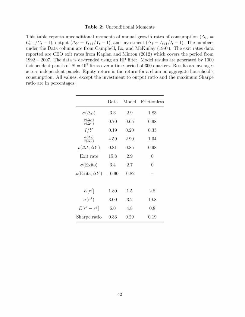
Table 2: Unconditional Moments

This table reports unconditional moments of annual growth rates of consumption (∆C =Ct+1/Ct − 1), output (∆Y = Yt+1/Yt − 1), and investment (∆I = It+1/It − 1). The numbersunder the Data column are from Campbell, Lo, and McKinlay (1997). The exit rates datareported are CEO exit rates from Kaplan and Minton (2012) which covers the period from1992− 2007. The data is de-trended using an HP filter. Model results are generated by 1000independent panels of N = 105 firms over a time period of 300 quarters. Results are averagesacross independent panels. Equity return is the return for a claim on aggregate household’sconsumption. All values, except the investment to output ratio and the maximum Sharperatio are in percentages.

Data Model Frictionless

σ(∆C) 3.3 2.9 1.83

σ(∆C)σ(∆Y )

0.70 0.65 0.98

I/Y 0.19 0.20 0.33

σ(∆I)σ(∆Y )

4.59 2.90 1.04

ρ(∆I,∆Y ) 0.81 0.85 0.98

Exit rate 15.8 2.9 0

σ(Exits) 3.4 2.7 0

ρ(Exits,∆Y ) - 0.90 -0.82 –

E[rf ] 1.80 1.5 2.8

σ(rf ) 3.00 3.2 10.8

E[re − rf ] 6.0 4.8 0.8

Sharpe ratio 0.33 0.29 0.19

42

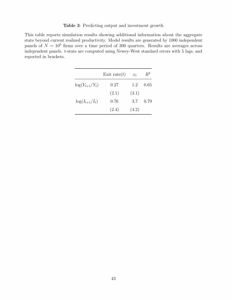
Table 3: Predicting output and investment growth

This table reports simulation results showing additional information about the aggregatestate beyond current realized productivity. Model results are generated by 1000 independentpanels of N = 105 firms over a time period of 300 quarters. Results are averages acrossindependent panels. t-stats are computed using Newey-West standard errors with 5 lags, andreported in brackets.

Exit rate(t) xt R2

log(Yt+1/Yt) 0.27 1.2 0.65

(2.1) (3.1)

log(It+1/It) 0.76 3.7 0.79

(2.4) (4.2)

43

Nature draws 𝑥𝑡1 − 𝛿 1 − 𝜒 𝑘

Investor Manager

Exit

𝛿𝑘

Nature draws 𝑧𝑡

𝑦𝑡 = 𝑥𝑡 + 𝑧𝑡 𝑘

𝑦𝑡 − 𝑑𝑡 𝑑𝑡(ℎ𝑡−1, 𝑠𝑡 , 𝑧𝑡)

Figure 1: Intra-period time-line of the model. The aggregate shock x is revealed at thebeginning of the period, after which the lottery for termination is held. A manager whosecontract is terminated receives nothing, while the investor recovers a fraction, (1 − χ), ofthe physical assets of the firm. If the manager continues, he receives maintenance cost δk.Production takes place when the firm-specific shock z is realized. The output y is dividedbetween the manager and investors. The period ends.

44

0 0.5 1 1.50

0.5

1

(V0, e)

V

F

0 0.5 1 1.50

0.5

1

1.5

2

2.5

F(V)

Rationed

Enter

H = hNt

V

eFigure 2: Entry condition of new managers into the economy. Panel A shows an example.The solid curve shows the investor’s value of a new contract as a function of promised utilityto the manager. The initial installation cost for this project is e0k. The contract is initiatedwith the manager getting a promised utility of V0. Panel B shows the same for all potentialentrants in the economy. A new firm requires a fixed installation cost ek to be paid. Thisrandom cost is drawn from a uniform distribution. Managers who draw a project cost lessthan the maximum contract value to the investor begin operations, while those with moreexpensive projects are rationed.

0 0.2 0.4 0.6 0.8 10

0.5

1 F(V)F(V)

V

F(V

)

Figure 3: Investor’s valuation of contract. The solid curve shows the investor’s value of futurecash flows from the contract as a function of the manager’s continuation value. For lowcontinuation value, the curve is increasing because increasing the manager’s continuation valuelowers the probability of termination. At high continuation value, increasing the manager’scontinuation value is a wealth transfer to the manager. This lowers the investor’s value.

45

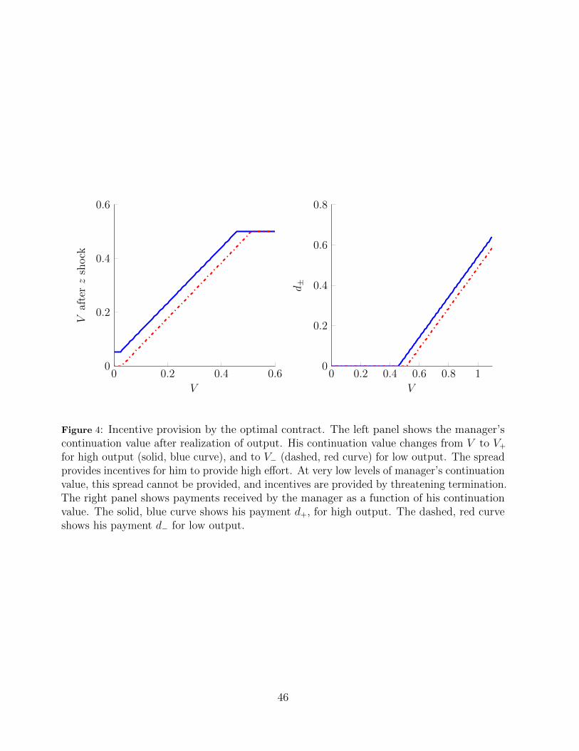
0 0.2 0.4 0.60

0.2

0.4

0.6

V

Vaf

terz

shock

0 0.2 0.4 0.6 0.8 10

0.2

0.4

0.6

0.8

V

d±

Figure 4: Incentive provision by the optimal contract. The left panel shows the manager’scontinuation value after realization of output. His continuation value changes from V to V+

for high output (solid, blue curve), and to V− (dashed, red curve) for low output. The spreadprovides incentives for him to provide high effort. At very low levels of manager’s continuationvalue, this spread cannot be provided, and incentives are provided by threatening termination.The right panel shows payments received by the manager as a function of his continuationvalue. The solid, blue curve shows his payment d+, for high output. The dashed, red curveshows his payment d− for low output.

46

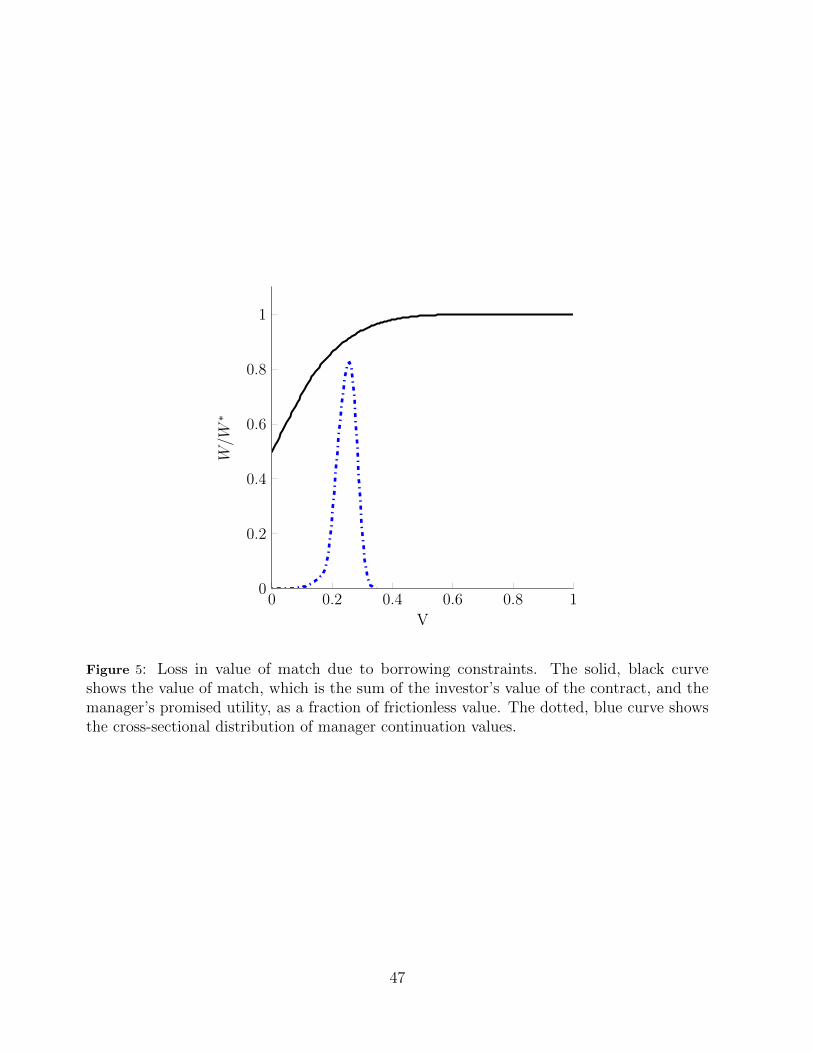
0 0.2 0.4 0.6 0.8 10

0.2

0.4

0.6

0.8

1

V

W/W

∗

Figure 5: Loss in value of match due to borrowing constraints. The solid, black curveshows the value of match, which is the sum of the investor’s value of the contract, and themanager’s promised utility, as a fraction of frictionless value. The dotted, blue curve showsthe cross-sectional distribution of manager continuation values.

47

0 0.2 0.4 0.6 0.80

1

2

3

4

5

6

V

µ

Figure 6: The steady-state distribution for two values of insider ownership measured byB/∆p(z+ − z−). The dotted black curve is for a lower value of B/∆p(z+ − z−) = 0.25, whilethe solid blue curve is for higher B/∆p(z+ − z−) = 0.40.

0 0.2 0.4 0.60

0.2

0.4

0.6

Initial V

Vaf

ter

stat

ech

ange

Figure 7: The change in continuation value when the state changes from boom to recession.

48

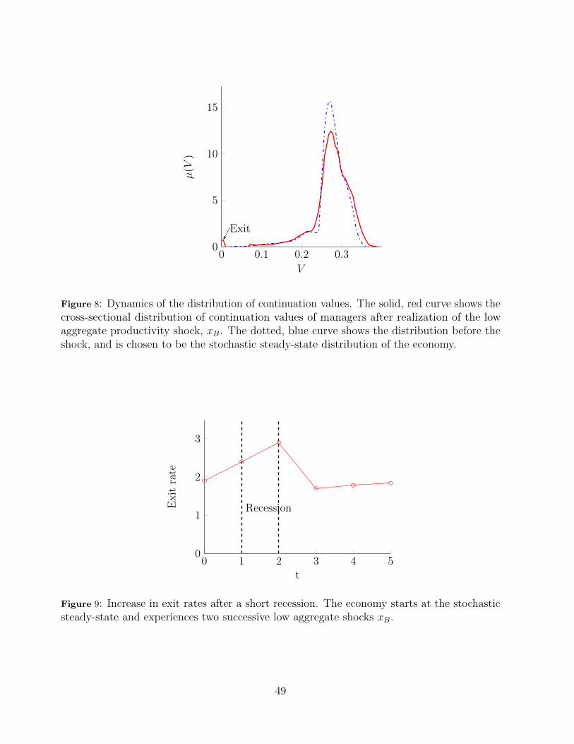
0 0.1 0.2 0.30

5

10

15

Exit

V

µ(V

)

Figure 8: Dynamics of the distribution of continuation values. The solid, red curve shows thecross-sectional distribution of continuation values of managers after realization of the lowaggregate productivity shock, xB. The dotted, blue curve shows the distribution before theshock, and is chosen to be the stochastic steady-state distribution of the economy.

0 1 2 3 4 50

1

2

3

Recession

t

Exit

rate

Figure 9: Increase in exit rates after a short recession. The economy starts at the stochasticsteady-state and experiences two successive low aggregate shocks xB.

49

0 1 2 3 4 50

0.1

0.2

0.3

Recession

t

Max

.Shar

pe

rati

o

Figure 10: Increase in the maximum Sharpe ratio after a short recession. The maximumSharpe ratio is the ratio of the volatility of the stochastic discount rate to its mean σ(π′)/E[π′].The economy starts at the stochastic steady-state and experiences two successive low aggregateshocks xB.

0 2 4 6 80

2

4

6

Recession

t

Exit

rate

Figure 11: Increase in exit rates after a long recession. The economy starts at the stochasticsteady-state and experiences five successive low aggregate shocks xB.

50

0 2 4 6 80

0.2

0.4

0.6

Recession

t

Max

.Shar

pe

rati

o

Figure 12: Increase in the maximum Sharpe ratio after a long recession. The maximum Sharperatio is the ratio of the volatility of the stochastic discount rate to its mean σ(π′)/E[π′]. Theeconomy starts at the stochastic steady-state and experiences five successive low aggregateshocks xB.

0 2 4 6 8 10 12 14 16 18 20−6

−4

−2

0

2

4

6·10−2

t

I

Figure 13: Response of aggregate investment to a one standard deviation shock in aggregateproductivity x. The dashed red curve shows the response to a negative shock, while the solidblue curve is the response to a positive shock. Notice the asymmetric response.

51

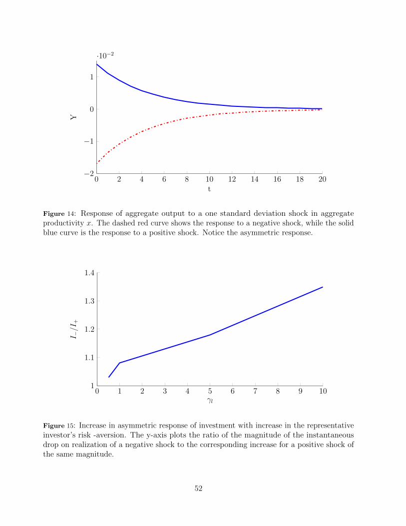
0 2 4 6 8 10 12 14 16 18 20−2

−1

0

1

·10−2

t

Y

Figure 14: Response of aggregate output to a one standard deviation shock in aggregateproductivity x. The dashed red curve shows the response to a negative shock, while the solidblue curve is the response to a positive shock. Notice the asymmetric response.

0 1 2 3 4 5 6 7 8 9 101

1.1

1.2

1.3

1.4

γl

I −/I

+

Figure 15: Increase in asymmetric response of investment with increase in the representativeinvestor’s risk -aversion. The y-axis plots the ratio of the magnitude of the instantaneousdrop on realization of a negative shock to the corresponding increase for a positive shock ofthe same magnitude.

52

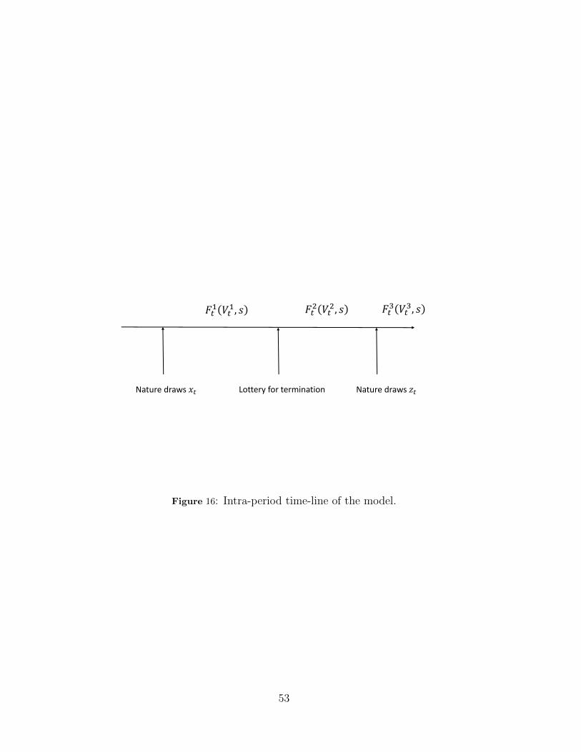
Nature draws 𝑥𝑡

𝐹𝑡1 𝑉𝑡

1, 𝑠 𝐹𝑡2 𝑉𝑡

2, 𝑠 𝐹𝑡3 𝑉𝑡

3, 𝑠

Lottery for termination Nature draws 𝑧𝑡

Figure 16: Intra-period time-line of the model.

53