1

Agglomeration, Spatial Interaction and Convergence in the EU Michael Bräuninger, Annekatrin Niebuhr

Abstract We investigate the convergence process among EU regions between 1980-2002 taking into

account the effects of spatial heterogeneity and spatial spillover effects. The spatial regimes

model allows for different steady-state growth paths. In contrast to previous analyses, the

regimes in this paper refer to spatial categories, i.e. we assume that agglomerations, urbanised

and rural regions are characterised by group-specific steady-states. Moreover, the regression

analysis considers the effects of interaction among neighbouring regions, possibly leading to a

spatial dependence of regional growth rates. We check whether spatial dependence is caused

by spatial spillovers or based on country effects.

JEL classification: C21, O52, R11

Keywords: Convergence, agglomeration, European Union, spatial econometrics,

quantile regression

Annekatrin Niebuhr IAB Nord: Regional Research Network of the Institute for Employment Research Projensdorfer Straße 82 D-24106 Kiel Germany e-mail: annekatrin.niebuhr@iab.de

Michael Bräuninger HWWA-Hamburg Institute of International Economics Neuer Jungfernstieg 21 20347 Hamburg Germany e-mail: michael.braeuninger@hwwa.de

Acknowledgements: We would like to thank Carsten Schürmann for the provision the travel time data and Cambridge Econometrics for the access to their regional databank. We are grateful to participants of the Spatial Econometrics Workshop 2005 at the Kiel Institute for World Economics for helpful comments on an earlier version of this paper.

2

1. Introduction

Regional growth and convergence are issues of intense research since the early 1990s initiated

at least partly by the development of New Growth Theory and New Economic Geography

(NEG). Both theories have important implications regarding the determinants of regional

growth and the evolution of regional disparities. Although considerable progress has been

made with respect to the knowledge on these issues still new aspects emerge. Recent

developments refer to theoretical as well as empirical research. Firstly, as regards advances in

theoretical research there are new approaches that incorporate endogenous growth in an NEG

framework. Corresponding analyses allow for interesting insights on the relationship between

agglomeration and growth. Studies by Martin and Ottaviano (2001) as well as Baldwin and

Forslid (2000) establish links between agglomeration, the evolution of regional income

differences and the level of overall growth.

Secondly, current empirical work emphasises the spatial dimension of growth and

convergence. The new theories stress the significance of spillover effects and there is growing

awareness that space matters for growth. Spatial effects are increasingly recognised as an

important feature of regional growth processes with a basis in economic theory. Spatial

econometric methods enable us to analyse the implication of new theoretical approaches in

this respect. Studies by Anselin et al. (1997), Bottazzi and Peri (2003), and Funke and

Niebuhr (2005) among others aim at investigating the impact of spatial spillover effects on

innovation, growth and regional disparities. Fingleton (2003) argues that spillovers might give

rise to spatial dependence of regional growth which has to be dealt with by spatial regression

models. Another strand of literature considers spatial heterogeneity in connection with

regional convergence. Quah (1996) investigates whether income growth of EU regions is

characterised by the formation of convergence clubs. Moreover, analyses by Baumont et al.

(2003) and Fischer and Stirböck (2004) indicate that convergence clubs exhibit specific

spatial patterns. They detect different spatial regimes in Europe that are characterised

generally speaking by a divide between Northwest and Southeast. Finally, Crozet and Koenig

(2004) investigate whether regional growth in the EU is marked by a tradeoff between growth

and cohesion. An implication of recent models that integrate endogenous growth and NEG is

that agglomeration, i.e. increasing regional disparities, can be a source of higher growth at the

national level.

However, empirical evidence on the various linkages between agglomeration, spillovers and

growth is still scarce. This paper aims at providing additional empirical findings on the

3

relevance of these interrelated phenomena. The analysis considers some of the above

mentioned issues. We analyse convergence among European regions between 1980 and 2002.

More precisely, the paper deals with the question whether convergence clubs, i.e. different

spatial regimes mark the development regional income disparities in Europe. In contrast to the

above mentioned studies, we define spatial regimes starting from a classification of spatial

categories. As a basic idea agglomerations and rural peripheral regions are marked by

different steady state equilibria and therefore constitute convergence clubs. We depart from

new theoretical models which focus on the link between agglomeration, growth and

convergence. This theoretical framework suggests considering both convergence clubs and

spatial dependence as potential features of regional growth in Europe.

Moreover, we focus on two statistical issues. As Temple (1999) notes many cross-section

growth regressions suffer from serious outliers. Outlying regions can have a marked effect on

OLS regression results and therefore more robust regressions might be appropriate. In

addition, Durlauf (2001) suggest that modelling parameter heterogeneity is one of the crucial

topics on the agenda for empirical growth modelling. To address the issues we apply quantile

regressions as introduced by Koenker and Basset (1978). Parameter heterogeneity across the

conditional distribution has been analysed by Barreto and Hughes (2004) at the country level.

To our knowledge, quantile regressions have so far not been used for European regional data.

The rest of the paper is organised as follows. In section 2, we briefly outline the theoretical

background of our empirical investigation. The main features and implications of recent

theoretical models which exhibit multiple equilibria and integrate NEG and endogenous

growth are summarised. The empirical methodology is introduced in section 3. Data and cross

section are described in section 4. In section 5, the regression results are presented. We

conclude with a summary of the main results in section 6.

2. Theory

Martin and Ottaviano (2001) note the relationship between growth and agglomeration is

already apparent in the changes that mark the industrial revolution in Europe. The sharp

increase in economic growth at that time was accompanied by urbanisation, the formation of

industrial clusters and increasing regional disparities. According to this observation

geography might matter for growth. Fujita and Thisse (2002) argue that agglomeration can be

considered as the territorial counterpart of growth. Moreover, the role of cities in economic

4

growth is emphasised. Cities might act as locations where technological and social

innovations are developed and, therefore, could be considered as engines of growth. Recently

theoretical models have been developed that allow analysing how growth and location impact

on each other.

In theoretical approaches that include endogenous growth in an NEG framework, growth and

agglomeration of economic activities are mutually self-reinforcing processes: growth brings

about agglomeration and agglomeration fosters growth (see Martin and Ottaviano 2001).

Models by Fujita and Thisse (2002) as well as Baldwin and Forslid (2000) combine the

Krugman core-periphery model with Romer-type endogenous growth. As a main result of

corresponding approaches, growth is affected by the spatial distribution of mobile skilled

workers who develop new goods in an R&D sector. More precisely, the overall growth rate of

the economy depends on the distribution of R&D activity across space. Knowledge capital

affecting the productivity of researchers positively is assumed to increase in each region with

the interaction of all skilled workers. The interaction among researchers in turn is influenced

by the spatial distribution of researchers. Proximity due to agglomeration fosters interaction

and innovation.

In general, the analyses differentiate between global and local knowledge spillovers. In case

of global spillover effects, i.e. patents for new goods and technological knowledge are

transferred costlessly among all regions, the R&D sector is located in a single region since

agglomeration forces are strong. Moreover, the industrial sector might be partly or fully

agglomerated in the same region. In the model by Ottaviano and Martin (1999), geography

will not affect growth, if spillovers are global. Determinants of growth such as the R&D cost

impact on regional income differentials and therefore on the location of firms. In this

framework, high growth is associated with convergence since factors that increase the growth

rate also decrease income differences.

If localised knowledge spillovers are assumed, e.g. because of important tacit knowledge,

R&D and industry tend to be entirely agglomerated in one region. R&D activities will move

to agglomerated regions, because with local spillovers R&D costs are lowest in

agglomerations where firms that produce differentiated products concentrate. Altogether, the

R&D sector represents a strong centripetal force that amplifies the cumulative causation.

Under specific assumptions the models imply that agglomeration fosters innovation and

growth. Agglomeration of skilled workers enables them to generate higher growth and a rate

of innovation. As in NEG models, agglomeration is associated with increasing disparities in

5

regional per capita income. Growth increases with the degree of industrial agglomeration and

hence diverging regional per capita income. Inequality can be a source of more growth, when

technological externalities are localised, as Crozet and Koenig (2004) put it. Thus the results

suggest a trade off between equity and growth. Both core and periphery enjoy higher growth,

but the income gap between centre and periphery increases.1 To a large extent, regional

income disparities reflect the geographical distribution of skills and differences between

agglomerations and rural peripheral regions.

However, there is another class of models which predict the existence of convergence clubs.

Club convergence can also be derived from growth models, such as in Azariadis and Drazen

(1990), which exhibit multiple steady state equilibria. In these kinds of models, the steady

state equilibrium of a region is determined by its initial conditions, and regions will converge

to the same steady state, if they are characterised by similar conditions. Several approaches

refer to human capital formation as a cause of club convergence.2 Due to social increasing

returns to scale from human capital accumulation, countries or regions differing with respect

to their initial level of human capital might converge to different steady state equilibria.

According to Canova (2004), several factors such as the endowment of important factors of

production (human capital, public infrastructure, R&D activity), preferences or government

policies may induce convergence clubs. As there are systematic differences between

agglomerations and rural peripheral regions with respect to human capital endowment,

infrastructure and R&D activity, these models reinforce theoretical arguments regarding

convergence clubs which correspond with spatial categories. However, the models also

provide arguments for an influence of national factors as national policies or legislation.

With respect to an empirical analysis of regional growth the implications of the models stress

primarily two aspects. Firstly, the theoretical models suggest that centre and periphery might

not converge to the same steady state, and we should therefore check the existence of

convergence clubs. Secondly, the theoretical approaches point at the significance of spillover

effects and the relevance of their geographical range as regards the development of regional

disparities. Geographic spillover effects might be considered explicitly by spatial regression

models.

1 However, from a welfare point of view the periphery might still be better off in the agglomeration case,

even without transfers, provided the growth effect of agglomeration is strong enough. 2 See Galor (1996) for a survey of different models that generate club convergence.

6

3. Methodological aspects

Our methodology assumes that the core-periphery pattern considered by Fujita and Thisse

(2002) as well as Ottaviano and Martin (1999) does not refers to the European scale as e.g. a

corresponding scheme proposed by the EU Commission (2001).3 In our opinion the approach

is more appropriate to explain differences between highly agglomerated urban regions and

rural peripheral areas. Therefore the empirical analysis investigates convergence among

different spatial categories: agglomerated regions, urbanised regions and rural regions. This is

in contrast to recent analyses of convergence among European regions by Fischer and

Stirböck (2004) as well as Baumont et al (2003). These authors also apply a spatial regimes

approach, but define categories similar to the European core-periphery pattern suggested by

the Commission. Moreover, there is a second difference between our approach and the above

mentioned convergence studies. Whereas they estimate both regime-specific intercepts and

convergence rates, we only consider different intercepts by including corresponding dummy

variables.

In their cross-country growth analysis Durlauf and Johnston (1995) argue that economic

theory provides no information on the number of regimes or the way in which variables

determine the different convergence clubs. Therefore they apply a data-sorting method in

order to select the regimes endogenously. As Baumont et al. (2003) note, a corresponding

methodology that takes into account spatial effects is not available yet. Moreover, the

theoretical models outlined in section 2 supply some hints as regards the determination of

convergence clubs. They imply the non convergence of per capita income of the centre and

the periphery. The concept of convergence clubs is in line with such persistent disparities.

Transferred to the European economic landscape, the theoretical framework suggests

differentiating between highly agglomerated regions, being the origin of innovation and

growth, on the one hand side and rural peripheral regions where no or only little R&D takes

place on the other hand. The latter regions might benefit from growth and innovation initiated

in the agglomeration, but they will not be able to catch up to the income level of

agglomerations if spillovers are not global.

A common approach to investigate regional convergence is the traditional cross-sectional

regression with income growth )/ln( tTt yy + as dependent variable and the initial level of

income )ln( ty as explanatory variable. We also include a number of dummy variables in

3 EU Commission (2001), map A.4.

7

order to account for national factors and effects specific to different region types. Using

matrix notation, the corresponding conditional convergence model is given by:

0 11 t T

tt

yln ln( y ) ST y

α ι α γ ε+� �= + + +� �

� �

Here S represents the matrix of country and region type dummies and γ is a vector of

coefficients. There is conditional convergence if 1 0α < . The rate of convergence β can be

obtained using the relation 11ln( T ) / Tβ α= − − . If ε ∼ ),0( 2INV σ , OLS will be blue. Given

that our data is a cross section of regions we might have three types of departures from this

assumption: Firstly, there might be heteroskedasticity; secondly, there might be spatial

autocorrelation, and thirdly, there might be outliers and parameter heterogeneity. While the

first deviation leads inefficiency of OLS, the last two might seriously bias the estimates.

To deal with all three issues we proceed in three steps: first we estimate OLS. Using the

RESET and the White-test we check for misspecification and heteroskedasticity. To measure

spatial autocorrelation in regression residuals, we use a number of different tests: a Moran test

and Lagrange Multiplier tests (LMLAG, LMERR and robust versions of tests). The Moran test

provides results for alternative forms of ignored spatial dependence, whereas the LM tests

supply precise information about the kind of spatial dependence (see Anselin/Rey 1991,

Anselin/Bera 1998, Anselin/Florax 1995). According to the results of these tests, different

spatial models can be estimated if necessary, i.e. in case of a misspecification.4

Spatial effects are not accounted for explicitly in the regression model that we applied to

investigate conditional convergence and convergence clubs. However, ignoring spatial

dependence might result in serious econometric problems. A corresponding misspecification

will be reflected by spatially autocorrelated residuals. Anselin/Rey (1991) differentiate

between substantive spatial dependence and nuisance dependence. The latter refers to spatial

autocorrelation that pertains to the error term and can be caused by measurement problems,

such as a poor match between the spatial pattern of the analysed economic phenomenon and

the units of observation. The substantive form of dependence can be induced by the various

economic linkages that exist among neighbouring regions.

4 See Anselin (1988) for a detailed description of test statistics and spatial regression models.

8

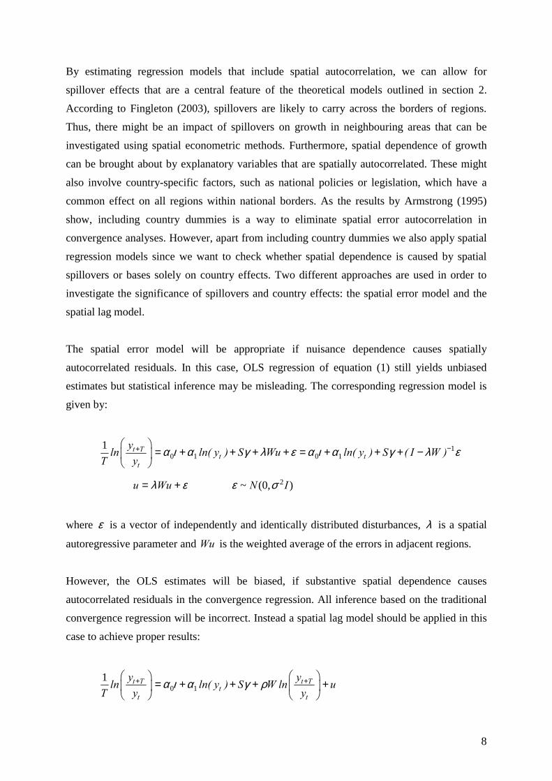
By estimating regression models that include spatial autocorrelation, we can allow for

spillover effects that are a central feature of the theoretical models outlined in section 2.

According to Fingleton (2003), spillovers are likely to carry across the borders of regions.

Thus, there might be an impact of spillovers on growth in neighbouring areas that can be

investigated using spatial econometric methods. Furthermore, spatial dependence of growth

can be brought about by explanatory variables that are spatially autocorrelated. These might

also involve country-specific factors, such as national policies or legislation, which have a

common effect on all regions within national borders. As the results by Armstrong (1995)

show, including country dummies is a way to eliminate spatial error autocorrelation in

convergence analyses. However, apart from including country dummies we also apply spatial

regression models since we want to check whether spatial dependence is caused by spatial

spillovers or bases solely on country effects. Two different approaches are used in order to

investigate the significance of spillovers and country effects: the spatial error model and the

spatial lag model.

The spatial error model will be appropriate if nuisance dependence causes spatially

autocorrelated residuals. In this case, OLS regression of equation (1) still yields unbiased

estimates but statistical inference may be misleading. The corresponding regression model is

given by:

10 1 0 1

1 t Tt t

t

yln ln( y ) S Wu ln( y ) S ( I W )T y

α ι α γ λ ε α ι α γ λ ε−+� �= + + + + = + + + −� �

� �

ελ += Wuu ),0(~ 2IN σε

where ε is a vector of independently and identically distributed disturbances, λ is a spatial

autoregressive parameter and Wu is the weighted average of the errors in adjacent regions.

However, the OLS estimates will be biased, if substantive spatial dependence causes

autocorrelated residuals in the convergence regression. All inference based on the traditional

convergence regression will be incorrect. Instead a spatial lag model should be applied in this

case to achieve proper results:

0 11 t T t T

tt t

y yln ln( y ) S W ln uT y y

α ι α γ ρ+ +� � � �= + + + +� � � �

� � � �

9

1 10 1 t( I W ) ( ln( y ) S ) ( I W ) uρ α ι α γ ρ− −= − + + + −

where ρ is the spatial autoregressive parameter of the spatially lagged dependent variable.

Finally, we have to consider that OLS and spatial regressions can be seriously biased by

outliers. Given that measurement at the regional level is conceptually and practically difficult,

mismeasurements seems to be likely. Therefore, the robustness to outliers is rather important

in the regional context. Another problem arises if the influence of explanatory variables

changes in the growth process. To deal with outliers and parameter heterogeneity we use

quantile regressions as introduced by Koenker and Basset (1978) and surveyed by Koenker

and Hallok (2001). The 0.5-quantile regression, i.e. the median regression, corresponds to

least absolute deviation estimator and is, therefore, a robust alternative to OLS. Minimizing

the distance to other quantiles than the median, gives an estimate for the marginal effects of a

change in the independent variables at the particular point of the conditional distribution (see

Buchinsky 1998). Typically, quantile regressions have been applied to micro data. As an

exception, Barreto and Hughes (2004) analyse convergence at the country level and find

considerable parameter heterogeneity across the conditional distribution.

Quantile regressions minimize an objective function which is a weighted sum of absolute

deviations:

{ }( )

{ }1

i i i i

k i i i ii i:y x i i:y x

min g x g xβγ γ

τ γ τ γ∈∈ ≥ ∈ <

� �� �− + − −� �� �

� �

Here gi= (log(yt+T) � log(yt))/T is the average annual growth rate and xi is the vector of

explanatory variables which is multiplied by the coefficients γ. Here explanatory variables

include country dummies, region types and initial income. The objective function can be

interpreted as an asymmetric linear penalty function of deviations from predicted to actual

growth rates. An important special case is the median regression (τ = 0.5) which gives the

least absolute deviations estimator. Since this regression puts less weight on outliers than

OLS, it is a robust alternative. Further, complete quantile regression yields a family of

coefficients; one for each sample quantile. Recent inferential procedures developed by

Koenker and Xiao (2001) allow to test hypotheses on the entire conditional distribution of

GDP per capita growth rates. This means that we are abele to test, whether the marginal

10

effects of a change in the independent variable are different at different quantiles of the

distribution.

4. Data

The paper aims to investigate the significance of national factors, region types and spatial

effects for growth and convergence in the EU. Starting from our theoretical considerations,

we have to deal primarily with three types of effects:

• Country specific effects: Economic policies, legislation and institutions tend to be the

same for all regions within a specific country. However, they usually differ across

countries. If policy and institutions in country A promote growth better than those in

country B, country A should grow at a higher rate.

• Region type effects: Agglomerations, urbanised and rural regions differ not only with

respect to their population density. Among other things, they are also marked by

different human capital endowments and R&D activity. Since these are important

determinants of growth, the disparities may affect long-run growth and convergence.

Hence, there might be systematic differences between growth rates of region types.

• Spatial effects: Recent research emphasises the significance of spillover effects for

economic growth. As the impact of spillovers might exceed regional boundaries,

growth of neighbouring areas is possibly marked by spatial dependence.

The following data description is structured by the three different kinds of regional specific

effects. We analyse of growth in 192 European regions over the period 1980 – 2002. The

regional per capita GDP series are drown from Cambridge Regional Economics data. The 192

NUTS 2 regions are form 15 EU countries: Austria AU (9), Belgium BE (11), Germany DE

(30), Denmark DK (3), Spain ES (16), Finland FI (5), France FR (22), Greece GR (13),

Ireland IE (2), Italy IT (20), Luxemburg LU (1), Netherlands NE (10), Portugal PT (5),

Sweden SE (8), Spain ES (16), United Kingdom UK (37).

Differences in the growth experience of EU countries are well documented in the literature.

Average annual growth rates between 1980 and 2002 are in the rage of 1.3% in Greece and

4.8% in Ireland. The box and whisker plot in Figure 1 shows the distribution of average

annual growth rates across and within countries. For each country the box represents the

middle half of the distribution of growth rates. The horizontal line represents the median

11

growth rate. The whiskers display the lower and the upper quartile of the distribution. In cases

where regions require whiskers exceeding 1.5 they are truncated and the remaining regions

are displayed as outliers. Three things become apparent from Figure 1. Firstly, Ireland and

Luxemburg are exceptions and systematically different from the other thirteen countries.

Secondly, the variation of regional growth rates within most countries is far higher than the

variation of median growth rates among the majority of countries. Thirdly, the plot reveals

seven regions with growth rates that are compared to their country distribution unusually high

or low.

<Box plot>

In order to analyse whether agglomerations and rural regions converge to different steady

states, we use a partition of EU regions into spatial categories. This classification is based on

a typology of settlement structure established by the Study Program on European Spatial

Planning.5 Based on the criteria population density and size of regional centres three groups of

regions (agglomerated, urbanised and rural regions) and six spatial categories have been

defined (see Table 1). The highly agglomerated areas with a large centre (agglomerated

regions, type 1) mainly comprise the capital regions of the EU member states. Moreover, this

group includes regions with large economic centres as e.g. the Ruhr area, parts of northern

Italy and southern Germany. Compared to type 1 the agglomerated regions of type 2 have a

lower population density (between 150 and 300 inhabitants per km2). They also contain some

European capitals (Lisbon and the Stockholm region). Urbanised and agglomerated areas are

first of all located in the core region of the EU, extending from the Southwest of the UK to

Belgium, the Netherlands and West Germany. In contrast, rural areas concentrate in the

periphery of the EU, i.e. especially the northern part of Sweden and Finland, Spain, Portugal

and Greece.

<Table 1>

Figure 2 displays a box and whisker plot for the distribution of growth rates across different

region types. According to the box plots there seems to be no systematic difference between

growth rates of different region types. The median growth rates are at about the same level

and they vary unsystematically between region types. In particular there is no tendency of

rural or urbanised regions to grow faster than agglomerations. This indicates that the different

5 See SPESP indicator set: http://www.bbr.bund.de/raumordnung/europa/espon.htm

12

region types might converge to different income levels. Within the unconditional framework,

the box and whisker plots reveal 5 regions with unusually high or low growth rates.

<Box plot>

Finally, we consider the spatial dimension of regional growth and investigate the spatial

autocorrelation of growth rates. Spatial autocorrelation describes the relation between the

similarity of a considered indicator and spatial proximity. Anselin (1988) notes that it is

generally taken to mean the lack of independence among observations in cross-sectional data

sets. Thus, positive spatial autocorrelation implies a clustering in space. Similar growth rates,

either high or low, are more spatially clustered than could be caused by chance.

Measures of spatial autocorrelation take into account the various directions of dependence by

a spatial weights matrix W. For a set of R observations, the matrix W is a R × R matrix whose

diagonal elements are set to zero. The matrix specifies the structure and intensity of spatial

effects. Hence, the element wij represents the intensity of effects between two regions i and j

(see Anselin/Bera 1998). A frequently applied weight specification is a binary spatial weight

matrix such that wij = 1 if the regions i and j share a border and wij = 0 otherwise. We apply

two additional concepts for spatial distance: In the first, we use the inverse of travel time

between region’s capitals for wij. In the second, we use the inverse of travel time for regions

within the same country and set wij = 0 for regions located in different countries. Table 2

presents the tests for spatial autocorrelation for regional growth, the log of initial income and

for the region types. The results indicate considerable spatial autocorrelation in European

regional growth and its potential determinants.

<<Table 2>>

5. Regression results We start with a general specification of the convergence regression including dummies for all

countries as well as for region and sub region types. The dependent variable is average annual

GDP per capita growth in percent. Table 3 gives the results for the OLS regression over the

sample period 1980 to 2002. The lower part of the table gives some regression diagnostics.

Since these indicate heteroskedastisity, we compute robust standard errors. The coefficient of

13

initial income is significantly negative. The dummies for urbanised and rural regions (R2 and

R3) are both significant and imply a lower steady state income level compared to

agglomerations. However, the dummies for the sub-regions (i.e. R1.2, R.2.2., R3.2) are

insignificant. Considering the country effects the OLS regression shows 5 countries (AT, BE,

DK, IE, LU) with significant positive coefficients, which implies a higher steady state income

level than in the reference country Germany. For Greece (GR) we obtain a negative

coefficient. In the lower part of the table the regression diagnostics are given. Here the

RESET and the White test indicate omitted variables or misspecification. The Lagrange

Multiplier tests (LM) and Robust Lagrange Multiplier tests (RLM) indicate that there are no

spatially autocorrelated residuals. Only Moran's I points to spatial autocorrelation. However,

results by Anselin and Rey (1991) suggest that the Moran statistic picks up a range of

misspecification errors, such as non-normality and heteroskedasticity and might therefore

provide unreliable inference. To assure that the non correlation of errors does not depend on

the specific form of the spatial weights matrix chosen, we use two alternative measures for

distance and binary weights. The tests of spatial correlation are recalculated with the binary

weights matrix and with the distance matrix cut off at the boarders. In both cases we cannot

find significant spatial autocorrelation in the error terms.

<<Table 3>>

Before we further investigate the question of spatial autocorrelation we eliminate insignificant

variables to reach a more parsimonious specification. The OLS estimation results for the

parsimonious specification are given in column 2 of Table 4. The regressions diagnostics in

the lower part of the table again indicate some misspecification. The Lagrange Multiplier tests

for spatial autocorrelation indicate no correlation of residuals. Still we estimate the spatial lag

and the spatial error model to check for the robustness of our results. The estimates are given

in columns 3 and 4 of Table 4. The coefficient of the initial income level is always

significantly negative and, therefore, evidence of conditional convergence is fairly robust. The

estimated speed of convergence is just below 1%. Furthermore, the findings imply

convergence to lower steady state levels for urbanised and rural areas and significant country

effects. In contrast, evidence of spatial effects is rather weak. In the spatial lag specification,

the coefficient ρ of the spatially lagged dependent variable is not significant. The coefficient λ

of the spatial error specification is not significant at the 5% level as well. According to

unreported regression results country-specific effects capture the spatial dependence that

marks regional growth of GDP per capita. Whereas the omission of county dummies leads to

14

considerable spatial autocorrelation, removal of the region type effects does not induce a

misspecification due to ignored spatial effects.6

Finally, even though the results of most coefficients estimates are remarkably stable over the

different specifications there remains some doubt: in all specification tests regression

diagnostics indicate heteroskedasticity or misspecification. The examination of standardised

residuals reveals several outliers. These might be the reason for the misspecification indicated

by the regression diagnostics. Since outliers can seriously bias OLS estimates, a more robust

regression technique is warranted.

In order to deal with the effects of outlying observations, we apply quantile regressions. We

start with the median regression, i.e. with the regression that gives the least absolute

deviations estimator and, therefore, the robust alternative to OLS.7 Again, we first estimate the

general model including all country dummies and sub region types as explanatory variables.

Then we eliminate all insignificant variables. We turn up with the same set of country

dummies as with OLS, and the sub region dummies are not significant. The results are given

in Table 5. In addition the table displays the results for regressions minimising the weighted

sum of deviations to the 10th, 25th, 75th and 90th quantile.

According to the median regression given in column 4 of Table 5, the same explanatory

variables as with OLS are significant. Furthermore, the marginal effects of these variables on

the regional growth rates are in the same order of magnitude. The initial income level is

significantly negative and so there is conditional convergence. The region type effects are

significant, implying that urbanised and rural regions converge to lower steady state levels

than agglomerations. Overall the median quantile estimator is rather similar to the OLS. This

result is quite reassuring since it means that the regression minimizing the distance to the

conditional mean leads to similar results as the regression minimizing the distance to median.

Since the median regression is robust to outliers, we can note that there is no serious bias

caused by outliers.

Now consider the estimates at other parts of the conditional distribution. As the comparison of

the results for different quantiles reveals that not all of the explanatory variables are

significant over all quantiles. However, the coefficient for the initial income is significantly

negative in all quantile regressions. Accordingly, even for regions where the model

6 Corresponding results are available from the authors upon request. 7 For an overview on quantile regressions see Buchinsky (1998).

15

underestimates the growth rate and for those regions where the model overestimates the

growth rate, there is convergence. The influence of region types differs across the different

quantiles. At the 10th quantile urbanised and rural areas are not significantly different to

agglomerations. Hence poor growth performance - relative to our model - appears

independent of the settlement structure.

<<Table 5 >>

Conclusions

Our results confirm the empirical evidence provided by a number of convergence studies:

income growth of European regions is characterised by convergence. Moreover, the findings

are in line with recent theoretical literature that combines endogenous growth with an NEG

framework. According to these models we might observe convergence clubs. More precisely,

agglomerations and rural peripheral regions possibly converge towards different steady state

equilibria. The findings of the present study suggest a lower steady state income level for

urbanised and rural areas of the EU than for highly agglomerated regions. At first sight this

evidence seems to conflict with recent empirical evidence provided by Baumont et al. (2003)

as well as Fischer and Stirböck (2004). These authors identify convergence clubs that refer to

centre and periphery at the European scale. In contrast, our differentiation applies to a lower

spatial scale and distinguishes agglomerations, urbanised and rural regions. However, there

are some similarities among both concepts. The incidence of spatial categories is linked to the

location in the centre and periphery at the European scale. Whereas rural areas are mainly

located in the periphery of the EU, urbanised regions and agglomerations concentrate in the

core region of Europe.

With respect to the significance of spatial dependence of regional growth caused by spillover

effects that affect income growth in neighbouring regions, the evidence in our study is rather

weak. Spatial autocorrelation seems to be mainly due to country-specific effects. Therefore,

regarding the importance of national factors as opposed to spatial-spillover factors we do not

agree with the assessment by Quah (1996), who concludes that spatial spillover factors matter

more than national factors. Spatial effects have undoubtedly significant growth effects. But

much of the spatial dependence that marks regional growth in Europe seems to base on

differences in national policies, legislation and institutions. However, there might be

important short-distance spillovers and growth dependencies among neighbouring regions

that we can not observe at our level of spatial aggregation.

16

References Anselin L (1988) Spatial Econometrics: Methods and Models. Dordrecht Anselin L, Bera A K (1998) Spatial Dependence in Linear Regression Models with an Introduction to Spatial Econometrics. In: Giles D, Ullah A (Eds.) Handbook of Applied Economic Statistics, Marcel Dekker, New York, 237-289 Anselin L, Florax J G M (1995) New Directions in Spatial Econometrics: Introduction. In: Anselin L, Florax J G M (Eds.) New Directions in Spatial Econometrics. Springer, Berlin, Heidelberg, New York, 21-74 Anselin L, Rey S (1991) Properties of Tests for Spatial Dependence in Linear Regression Models. Geographical Analysis 23, 112-131. Anselin L, Varga A, Acs Z (1997) Local Geographical Spillovers between University Research and High Technology Innovations. Journal of Urban Economics 42.3, 422-448. Armstrong HW (1995) Convergence among Regions of the European Union: 1950 - 1990. Papers in Regional Science 74, 143-152. Azariadis C, Drazen A (1990) Threshold externalities in economic development. Quarterly Journal of Economics 105, 501-526. Baldwin RE, Forslid R (2000) The Core-periphery Model and Endogenous Growth: Stabilizing and Destabilizing Integration. Economica 67, 307-324. Barreto, RA., Hughes, AW (2004) Under Performers and Over Achievers: A Quantile Regression Analysis of Growth. Economic Record 80, 17-35. Baumont C, Ertur C, Le Gallo J. (2003) Spatial Convergence Clubs and the European Regional Growth Process, 1980-1995. In: Fingleton B (Ed.), European Regional Growth, Springer, Berlin, Heidelberg, New York, pp. 131-158. Bottazzi L, Peri G (2003) Innovation and Spillovers in Regions: Evidence from European Patent Data. European Economic Review 47, 687-710. Buchinsky, M. (1994) Recent Advances in Quantile Regression Models. A Practical Guideline for Empirical Research. Journal of Human Ressources 33, 88 – 126. Canova F (2004) Testing for Convergence Clubs in Income per Capita: a Predictive Density Approach. International Economic Review 45, 49-78. Canova F (2001) Are EU Policies Fostering Growth and Reducing Regional Inequalities? Opuscle del CREI No. 8, 2001, Universitat Pompeu Fabra. Commission of the European Communities (2001): Unity, Solidarity, Diversity for Europe, its People and its Territory. Second Report on Economic and Social Cohesion, Luxembourg. Crozet M, Koenig P (2004) The Cohesion versus Growth tradeoff: Evidence from EU Regions (1980-2000), (http://team.univ-paris1.fr/teamperso/crozet/trade_off.pdf). Durlauf, S. (2001) Manifesto for a Gowth Eonometrics. Journal of Econometrics 100, 65-69.

17

Durlauf SN, Johnston PA (1995) Mutiple Regimes and Cross-country Growth Behaviour. Journal of Applied Econometrics 10, 365-384. Fingleton, B (2003) Models and Simulations of GDP per Inhabitant across Europe�s Regions: A Preliminary View. In: Fingleton B (Ed.), European regional growth, Springer, Berlin, Heidelberg, New York, pp. 11-53. Fischer M, Stirböck C (2004) Regional Income Convergence in the Enlarged Europe, 1995-2000: A Spatial Econometric Perspective, Centre for European Economic Research, Discussion Paper No. 04-42. Fujita M, Thisse J-F (2002) Economics of Agglomeration. Cities, Industrial Location, and Regional Growth. Cambridge University Press, Cambridge. Funke M, Niebuhr A (2005) Regional Geographic R&D Spillovers and Economic Growth: Evidence from West Germany. Regional Studies 39.1, 143-153. Galor O (1996) Convergence? Inferences from Theoretical Models. Economic Journal 106, 1056-1069 Koenker, R, Bassett, G (1978) Regression Quantiles. Econometrica 46, 33 – 50. Koenker, R, Hallok, KF (2001) Quantile Regression. Journal of Economic Perspectives 15, Fall 143 – 156. Koenker, R, Xiao, Z. (2002) Inference on the Quantile Regression Process, Econometrica, 70, 1583-1612. Martin P, Ottaviano GIP (2001) Growth and Agglomeration. International Economic Review 42, 947-968. Martin P, Ottaviano GIP (1999) Growing Locations: Industry Location in a Model of Endogenous Growth. European Economic Review 43, 281-302. Quah, D (1996) Regional Convergence Clusters across Europe. European Economic Review 40, 951-958. Temple, J (1999) The New Growth Evidence, Journal of Economic Literature 37, 112-156.

18

-20

24

6gr

owth

rate

s

AT BE DE DK ES FI FR GR IE IT LU NL PT SE UKDistribution of growth rates within and across countries

Box Plot

-20

24

6gr

owth

rate

s

1.1 1.2 2.1 2.2 3.1 3.2Distribution of growth rates within and across region types

Box Plot

19

Table 1: Spatial categories according to settlement structure Type Spatial categories Size of the regional centre

(number of inhabitants) Population density (inhabitants per km²)

Agglomerated regions

1.1 Highly agglomerated with large centre

> 300.000 > 300

1.2 Agglomerated with large centre > 300.000 150 up to 300

Urbanised regions

2.1 Urbanised with large centre < 300.000 or > 300.000

> 150 (and a centre with < 300.000 inhabitants)

or

100 up to 150 (and a centre with > 300.000 inhabitants)

2.2 Urbanised without large centre < 300.000 100 up to 150

Rural regions

3.1 Low population density and centre > 125.000 < 100

3.3 Low population density without centre

< 125.000 < 100

Table 2: Spatial correlation

Travel Time Travel Time cut at border Binary

Variable Moran's I Geary's c Moran's I Geary's c Moran's I Geary's c (ln(yt+T) � ln(yt))/T 0.054 0.901 0.412 0.588 0.179 0.803

(8.993) (-3.276) (13.458) (-10.543) (3.473) (-2.842)ln(yt) 0.206 0.737 0.704 0.281 0.468 0.556

(31.432) (-16.71) (22.453) (-21.522) (8.78) (-7.686)Region type 0.098 0.882 0.334 0.679 0.294 0.699

(15.335) (-10.7) (10.7) (-9.966) (5.538) (-5.43)z-ratios in parentheses

20

Table 3: Results of the general specification*

ln(yt) R1.2 R2 R2.2 R3 R3.2 -0.833 -0.074 -0.277 -0.013 -0.396 -0.095 (2.37) (0.47) (1.91) (0.11) (1.96) (0.72)

AT BE DK ES FI FR 0.486 0.262 0.577 0.32 0.489 0.077 (3.79) (1.63) (4.2) (1.12) (1.25) (0.56)

GR IE IT LU NL PT -0.636 2.829 -0.182 2.884 0.063 0.118 (1.58) (5.19) (0.83) (38.55) (0.21) (0.25)

SE UK const 0.081 -0.021 9.777 (0.31) (0.08) (2.78)

t-ratios in parentheses Regression diagnostics: R2 = 0.52; RESET: F(3, 168) = 9.64; White chi2(73) = 131.41; BP: chi2(1) = 5.14 Spatial error: Moran's I = 7.92 (0); LM = 0.84 (0.36); LM = 0.057 (0.81) Spatial lag: LM = 0.79 (0.38); RLM = 0.002 (0.97) * The dependent variable is the average annual growth rate in percent.

21

Table 4: Regression results*

OLS

Spatial lag

Spatial error

ln(yt)

-0.872

-0.811

-0.879

(6.44) (6.64) (7.54) R2 -0.258 -0.240 -0.275 (2.66) (2.61) (2.81) R3 -0.322 -0.313 -0.346 (3.09) (3.34) (3.57) AT 0.392 0.390 0.353 (4.29) (2.25) (1.89) BE 0.214 0.209 0.206 (1.77) (1.35) (1.19) DK 0.488 0.496 0.489 (5.06) (1.70) (1.67) GR -0.818 -0.711 -0.756 (4.22) (3.66) (3.97) LU 2.851 2.870 2.879 (34.39) (5.80) (5.88) IE 2.681 2.670 2.701 (5.52) (7.53) (7.51) IT -0.280 -0.248 -0.303 (3.27) (1.99) (2.19) Const. 8.897 8.897 10.256 (7.46) (5.34) (9.15) rho/lambda 0.393 0.636 (0.95) (1.93) R2 0.502 0.503 0.505

t-ratios in parentheses Diagnostics of the OLS Regression

RESET: F(3, 179) = 7.89; White chi2(27) = 37.07; BP: chi2(1) = 2.96 Spatial error: Moran's I = 5.28 (0); LM = 1.91 (0.17) ; RLM = 1.70 (0.19) Spatial lag: LM = 0.61 (0.43); RLM = 0.39 (0.53)

p-values in parentheses * The dependent variable is the average annual growth rate in percent.

22

Table 5: Quantile regressions*

10th 25th 50th 75th 90th ln(yt) -1.051 -1.039 -0.826 -0.965 -0.579 (3.94) (5.67) (7.88) (5.78) (1.91) R2 0.002 -0.261 -0.297 -0.235 -0.305 (0.01) (1.7) (3.94) (1.55) (1.64) R3 -0.261 -0.278 -0.304 -0.336 -0.225 (1.05) (1.96) (3.81) (2.52) (0.75) AT 0.729 0.558 0.31 0.411 -0.053 (5.73) (4.99) (2.74) (2.9) (0.22) BE 0.165 0.058 0.334 0.255 -0.047 (0.7) (0.22) (1.7) (1.63) (0.27) IT -0.217 -0.148 -0.313 -0.371 -0.546 (1.0) (1.15) (5.26) (3.04) (3.01) DK 1.176 0.759 0.414 0.381 -0.304 (3.85) (3.66) (3.2) (2.61) (0.95) GR -0.852 -0.934 -0.886 -0.667 -0.662 (1.98) (3.64) (4.80) (2.07) (2.09) IE 2.552 2.15 2.006 3.064 2.875 (2.16) (1.96) (1.77) (2.82) (2.77) LU 3.354 3.184 2.848 2.647 2.158 (2.08) (2.14) (2.12) (2.13) (2.1) Const. 11.156 11.465 9.764 11.255 8.049 (4.43) (6.38) (9.72) (7.04) (2.79) R2 0.234 0.249 0.300 0.305 0.349 The t-ratios in parentheses are based on standard errors bootstrapped with 200 replications

* The dependent variable is the average annual growth rate in percent.