Embed Size (px)
Citation preview

Agent Based Computational Finance: Suggested Readings and
Early Research ∗
Blake LeBaron
Graduate School of International Economics and Finance
Brandeis University
415 South Street, Mailstop 021
Waltham, MA 02453 - 2728
781 736-2258
October 1998
Abstract
The use of computer simulated markets with individual adaptive agents in finance is a new, but
growing field. This paper explores some of the early work in the area concentrating on a set of some of
the earliest papers. Six papers are summarized in detail, along with references to many other pieces of
this wide ranging research area. It also covers many of the questions that new researchers will face when
getting into the field, and hopefully can serve as a kind of minitutorial for those interested in getting
started.
∗The author is grateful to the Alfred P. Sloan Foundation for support. Cars Hommes provided useful comments on an earlierdraft.

1 Introduction
Modeling economic markets from the bottom up with large numbers of interacting agents is beginning
to show promise as a research methodology that will greatly impact how we think about interactions in
economic models. There is already a growing literature attempting to model financial interactions starting
from the agent perspective, relying heavily on computational tools to push beyond the restrictions of analytic
methods. This survey provides some pointers and synthesis on this new area of research.
Financial markets are an important application for agent based modeling styles. As with many other
economic situations, there is a great appeal in starting from the bottom up with simple adaptive, learning
agents.1 Beyond this, financial markets may offer other features which make them even more appealing
to agent based modelers. First, issues of price and information aggregation tend to be sharper in financial
settings where agent objectives tend to be clearer. Second, financial data is readily available at many
different frequencies from annual to minute by minute. Finally, there are continuing developments in the
area of experimental financial markets which give carefully controlled environments which can be compared
with agent based experiments. Financial markets have also posed many empirical puzzles for standard
representative agent models which have been unsatisfactory in explaining them.2
Computational agent based models stress interactions, and learning dynamics in groups of traders learning
about the relations between prices and market information. The use of heterogeneous agents is certainly not
new to finance, and there is a long history to building heterogeneous agent rational expectations models.3
What is attempted in this current set of computational frameworks is to attack the problem of very complex
heterogeneity which leaves the boundary of what can be handled analytically. Traders are made up from a
very diverse set of types and behaviors. To make the situation more complex the population of agent types,
or the individual behaviors themselves, are allowed to change over time in response to past performance.
Instead of trying to survey the literature, this paper will emphasize the results in six early papers. These
are chosen both because they are some of the earliest papers, and span an important realm of work in
artificial financial markets. In short, they are some of the most important papers that new researchers
should be aware of when they are just starting in this field. The next section will go through these brief1The best place for information on this is the web site maintained by Leigh Tesfatsion at Iowa State,
http://www.econ.iastate.edu/tesfatsi/ace.htm.2This list of puzzles includes rejections of the standard representative agent model, and the equity premium puzzle (Hansen
& Singleton 1983, Mehra & Prescott 1985, Hansen & Jagannathan 1990), volatility persistence (Bollerslev, Chou, Jayaraman& Kroner 1990), and the use and performance of technical trading rules (Brock, Lakonishok & LeBaron 1992, Levich &Thomas 1993, LeBaron 1998, Sweeney 1986). Kocherlakota (1996) is a recent survey of the large body of research on the equitypremium.
3Some of the origins of this are contained in Grossman (1976) and Grossman & Stiglitz (1980).
1
paper summaries. Any good survey should also give some of the key pointers to other papers in the area, and
it should be emphasized that the limitation in discussing only six papers was a severe binding constraint.
Some discussion and references will be made to the many other papers in this field in section three. While
the purpose of this paper was to concentrate on computational models, there are analytic approaches that
are closely related. Leaving out discussion of these papers would make this summary incomplete. The third
section also discusses a few of these papers along with the interactions between computational and analytic
approaches. The fourth section expands on the general survey of the paper by covering some of the issues
that need to be considered by anyone setting up their own computational experiments. Since this area is
new, there are still a large number of questions about market and agent design that remain unanswered. A
few of these issues will be discussed along with some suggestions for the future. The final section provides a
short conclusion.
2 Paper summaries
2.1 Simple agent benchmarks
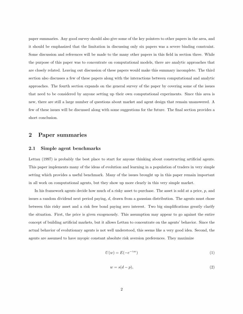
Lettau (1997) is probably the best place to start for anyone thinking about constructing artificial agents.
This paper implements many of the ideas of evolution and learning in a population of traders in very simple
setting which provides a useful benchmark. Many of the issues brought up in this paper remain important
in all work on computational agents, but they show up more clearly in this very simple market.
In his framework agents decide how much of a risky asset to purchase. The asset is sold at a price, p, and
issues a random dividend next period paying, d, drawn from a gaussian distribution. The agents must chose
between this risky asset and a risk free bond paying zero interest. Two big simplifications greatly clarify
the situation. First, the price is given exogenously. This assumption may appear to go against the entire
concept of building artificial markets, but it allows Lettau to concentrate on the agents’ behavior. Since the
actual behavior of evolutionary agents is not well understood, this seems like a very good idea. Second, the
agents are assumed to have myopic constant absolute risk aversion preferences. They maximize
U(w) = E(−e−γw) (1)
w = s(d − p), (2)
2

where s is the number of shares held of the risky asset, the agent’s only choice variable.
For a fixed distribution of d it is well known that the optimal solution for s will be a linear function of
the price, p, and the mean dividend d.
s∗ = α∗(d − p) (3)
Lettau is interested in how close evolutionary learning mechanisms get to this optimal solution.4
To do this he implements a genetic algorithm (GA) which is a common tool in many computational
learning models. The GA was developed by Holland (1975), and is a biologically inspired learning method.
A population of candidate solutions is evolved over time by keeping the best, removing the worst, and adding
new rules through mutation and crossover. Mutation takes old rules and modifies them slightly, and crossover
takes two good rules and combines them into a new rule.5 It is clear that a complete solution is described
by α, and a population of these can be maintained.
In the early era of GA’s researchers concentrated on implementations using bitstrings.6 Given that the
solutions here require real values, some kind of translation is needed. Lettau follows a common convention
of using the base two integer representation for a fraction between some max/min range,
α = MIN + (MAX − MIN)
∑Lj=1 µj2j−1
2L − 1, (4)
where µ is the bitstring for a strategy. Bitstrings are now mutated by flipping randomly chosen bits, and
crossover proceeds by choosing a splitting position in µ at random, and getting bits to the left of this position
from one parent, and right from the other.
This framework is not without some controversy. Learning and evolution takes place in a space that is
somewhat disconnected from the real one. For example, mutation is supposed to be concerned with a small
change in a behavioral rule. However, for this type of mapping one might flip a bit that could change holdings
by a large amount. Many papers in the GA area have moved to simply using real valued representations,
and appropriately defined operators rather than relying on mapping parameters. Lettau (and others) are
following the procedure of the early papers from computer science, and I believe most of the results would
not be sensitive to changing this, but it would be an interesting experiment.4In earlier working versions of this paper Lettau considered more complicated functional forms for s(d, p) in the learning
procedure.5The GA is at the heart of many of the models discussed here. It is really part of a family of evolutionary algorithms which
include evolutionary programming, evolutionary strategies, and genetic programming. As these various methods have beenmodified, the distinctions across techniques have become blurred. Fogel (1995) and Back (1996) give overviews of some of theseother evolutionary methods.
6See Goldberg (1989) for summaries.
3

A second critical parameter for Lettau is the choice of sample length to use for the determination of
fitness. A candidate rule, i, is evaluated by how well it performs over a set of S experiments,
Vi =S∑
j=1
Ui(wi,j), (5)
where wi,j is the wealth obtained by rule i in the jth experiment. Since fitness is a random variable, the
number of trials used to determine expected utility is critical. Extending S to infinity gives increasingly
more precise estimates of rule fitness.
In general, Lettau’s results show that the GA is able to learn the optimum portfolio weight. However,
there is an interesting bias. He finds that the optimal rules have a value for α which is greater than the
optimal α∗. This bias implies that they generally will be holding more of the stock than their preferences
would prescribe. This is because agents are choosing
α∗∗ = arg maxαi
S∑
j=1
Uαi(wj), (6)
and E(α∗∗) 6= α∗. Intuitively, the reason is quite simple. Over any finite sample, S, there will be a set of
rules that do well because they faced a favorable draw of dividends. Those that took risks and were lucky
will end up at the top of the fitness heap. Those that took risks and were unlucky will be at the bottom,
and the conservative rules will be in the middle. As the GA evolves, this continues to suggest a selection
pressure for lucky, but not necessarily skillful strategies. Pushing S to infinity exposes agents to more trials,
and the chances of performing well do to chance go to zero. Lettau shows that for very large S, the bias
does indeed get close to zero as expected.
This last feature of the GA in noisy environments carries over into many of the other papers considered
here. Deciding on fitness values to evolve over is a critical question, and almost all of the papers used here
are forced to make some decision about how far back their agents should look, and how much data they
should look at. This issue is probably not one that is specific to computerized agents, and is one that is not
considered enough for real life behavior in financial markets.7
7See Benink & Bossaerts (1996) for a version of this issue in an analytic framework.
4

2.2 Zero Intelligence traders
The next paper may not really be a move up the ladder of intelligence in terms of of agents, but it is another
crucial early benchmark paper with computational agents. After observing the behavior of many real trading
experiments in laboratories, Gode & Sunder (1993) were interested in just how much “intelligence” was
necessary to generate the results they were seeing. They ran a computer experiment with agents who not
only do not learn, but are almost completely random in their behavior.
The framework they are interested in is a double auction market similar to those used in many laboratory
experiments. Buyers can enter bids for an asset, or raise existing bids. Sellers can enter offers, or lower
existing offers. A match or cross of bids and offers implements a transaction. Value is induced as in Smith
(1976), where buyer i is given a redemption value of vi for the asset and therefore a profit of vi − pi from a
purchase at price pi. Sellers are given a cost to obtain the asset of ci, and therefore a profit of pi − ci. Note,
sellers and buyers do not overlap in these simple market settings. It is easy to evaluate efficiency of the
market by looking at the profits earned relative to the maximum possible. This is also the total consumer
and producer surplus in these markets.
The traders behavior is basically random, issuing random bids and offers distributed over a predefined
range. The authors implement one important restriction on their traders. They perform experiments where
the trader is simply restricted to his/her budget constraint. For example, a buyer would not bid more than
what the asset is worth in redemption value, and a seller will not offer below cost. Beyond this restriction
they continue to bid and offer randomly. Their results show that this budget constraint is critical.
Markets with human traders in the experiments are quite well behaved, often converging to the equilib-
rium price after only a few rounds. The random computer traders that are not subject to budget constraints
behave, as expected, completely randomly. There is no convergence, and transaction prices are very volatile.
The budget constrained traders behave quite differently, exhibiting a calmer price series which is close to
equilibrium. Market efficiency tests support these results by showing that the constrained traders allocate
the assets at over 97% efficiency in most cases which is very close to that for humans. The completely
random traders fall well back with efficiencies ranging from 50% to 100%.8
The message of this paper is critical to researchers building artificial markets. After a set of agents is
carefully constructed, it may be that subject to the constraints of the market they may be indistinguishable
from ZI traders. This means that researchers need to be very cautious about which features are do to learning8Recent work by Cliff & Bruten (1997) shows that the convergence to the equilibrium price may not occur in all market
situations. The relative slopes of the supply and demand curves are critical in determining how close the ZI agents get to theequilibrium price.
5

and adaptation, and which are coming from the structure of the market itself.
2.3 Foreign exchange markets and experiments
The following papers are more extensive than the first two in that they are attempting to simulate more
complicated market structures. Arifovic (1996) considers a general equilibrium foreign exchange market in
the spirit of Kareken & Wallace (1981). A crucial aspect of this model is that it contains infinitely many
equilibria because it is under specified in price space. Learning dynamics are often suggested as a means for
seeing if the economy will dynamically select one of these equilibrium prices (Sargent 1993).
The structure of the economy is based on a simple overlapping generations economy where two period
agents solve the following problem.
maxct,t,ct,t+1
log ct,t + log ct,t+1
st. ct,t ≤ w1 − m1,t
p1,t− m2,t
p2,t
ct,t+1 ≤ w2 +m1,t
p1,t+1+
m2,t
p2,t+1
The amounts m1,t and m2,t are holdings in the two currencies which are the only method for saving from
period 1 to 2, and can both be used to purchase the one consumption good. pi,t is the price level of currency
i in period t. Consumption, cm,n is for generation m at time n. The exchange rate at time t is given by,
et =p1,t
p2,t(7)
Finally, when there is no uncertainty the return on the two currencies must be equal,
Rt =p1,t
p1,t+1=
p2,t
p2,t+1. (8)
It is easy to show from the agent’s maximization problem that the savings demand of the young agents at t
is
st =m1,t
p1,t+
m2,t
p2,t=
12(w1 − w2
1Rt
) (9)
Given the returns on the currencies are equal, the agent is actually indifferent between which currency should
be used for savings. Aggregate currency amounts are assumed to be held constant for each country.
The basic indeterminacy in the model shown by Kareken & Wallace (1981) is that if there is a monetary
6
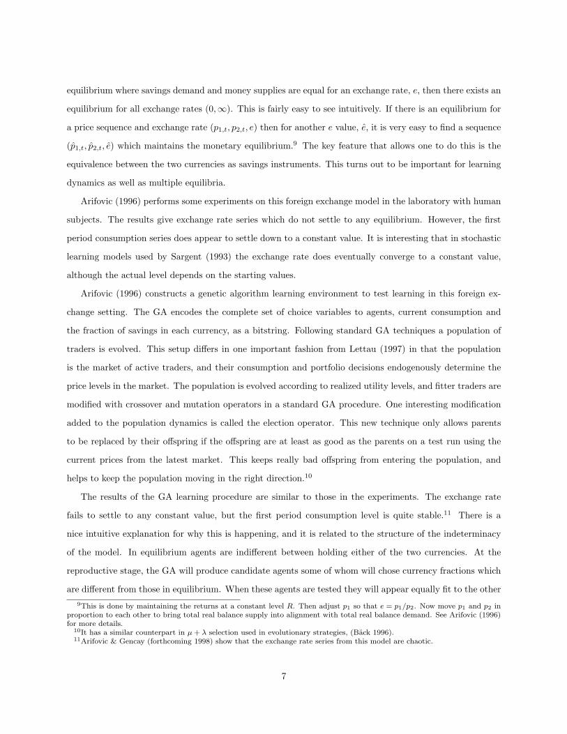
equilibrium where savings demand and money supplies are equal for an exchange rate, e, then there exists an
equilibrium for all exchange rates (0,∞). This is fairly easy to see intuitively. If there is an equilibrium for
a price sequence and exchange rate (p1,t, p2,t, e) then for another e value, e, it is very easy to find a sequence
(p1,t, p2,t, e) which maintains the monetary equilibrium.9 The key feature that allows one to do this is the
equivalence between the two currencies as savings instruments. This turns out to be important for learning
dynamics as well as multiple equilibria.
Arifovic (1996) performs some experiments on this foreign exchange model in the laboratory with human
subjects. The results give exchange rate series which do not settle to any equilibrium. However, the first
period consumption series does appear to settle down to a constant value. It is interesting that in stochastic
learning models used by Sargent (1993) the exchange rate does eventually converge to a constant value,
although the actual level depends on the starting values.
Arifovic (1996) constructs a genetic algorithm learning environment to test learning in this foreign ex-
change setting. The GA encodes the complete set of choice variables to agents, current consumption and
the fraction of savings in each currency, as a bitstring. Following standard GA techniques a population of
traders is evolved. This setup differs in one important fashion from Lettau (1997) in that the population
is the market of active traders, and their consumption and portfolio decisions endogenously determine the
price levels in the market. The population is evolved according to realized utility levels, and fitter traders are
modified with crossover and mutation operators in a standard GA procedure. One interesting modification
added to the population dynamics is called the election operator. This new technique only allows parents
to be replaced by their offspring if the offspring are at least as good as the parents on a test run using the
current prices from the latest market. This keeps really bad offspring from entering the population, and
helps to keep the population moving in the right direction.10
The results of the GA learning procedure are similar to those in the experiments. The exchange rate
fails to settle to any constant value, but the first period consumption level is quite stable.11 There is a
nice intuitive explanation for why this is happening, and it is related to the structure of the indeterminacy
of the model. In equilibrium agents are indifferent between holding either of the two currencies. At the
reproductive stage, the GA will produce candidate agents some of whom will chose currency fractions which
are different from those in equilibrium. When these agents are tested they will appear equally fit to the other9This is done by maintaining the returns at a constant level R. Then adjust p1 so that e = p1/p2. Now move p1 and p2 in
proportion to each other to bring total real balance supply into alignment with total real balance demand. See Arifovic (1996)for more details.
10It has a similar counterpart in µ + λ selection used in evolutionary strategies, (Back 1996).11Arifovic & Gencay (forthcoming 1998) show that the exchange rate series from this model are chaotic.
7

agents since in equilibrium the returns on the two currencies are the same. However, once these agents are
added to the population the prices will have to change to adjust to the new currency’s demands. The system
will then move away from the equilibrium, as this will probably move the two returns out of alignment. The
basic result is that because agents are indifferent between currency holdings, the equilibrium is subject to
invasion by nonequilibrium agents, and is therefore unstable under GA based learning.
This paper introduces several important issues for artificial markets. First, it is considering the equilib-
rium in a general equilibrium setting with endogenous price formation. Second, it compares the learning
dynamics to results from actual experimental markets as in Gode & Sunder (1993). Finally, it shows an inter-
esting feature of GA/agent based learning which appears to replicate certain features from the experiments
which can’t be replicated in other learning environments.
2.4 Costly information and learning
The next paper focuses on ideas of uncertainty and information in financial markets. Using the framework of
Grossman & Stiglitz (1980), Routledge (1994) implements a version of their model with GA based learning
agents. This paper takes us up another level of complexity in terms of model structure, and only a short
sketch of its details will be provided here.
The approach is based on a repeated one shot version of a portfolio decision problem with a costly
information signal that agents can decide to purchase. The dividend payout is given by
d = β0 + β1y + ε (10)
where y is the signal that can be purchased for a given cost, c. Agents are interested in maximizing expected
one period utility given by,
E(−e−γw1 |Ω) (11)
s.t. w1 = w0 − θc + x(d − p), (12)
with x being the number of shares of the risky asset. There is a risk free asset in zero net supply with
zero interest. θ is 1 for informed agents and 0 for uninformed. The expectation is conditioned on available
information. For the informed agents, it is price and the signal, y. For the uninformed, it is based on price
8

alone. With multivariate normality this leads to a demand for the risky asset of,
x =E(d|Ω) − p
γV (d|Ω). (13)
This demand is set equal to a noisy asset supply which represents noise trading, and keeps the underlying
signal from being fully revealed.
Learning takes place as the agents try to convert their information into forecasts of the dividend payout.
The informed build forecasts using the signal alone since the dividend payout is conditioned only on this,
En(d|y) = βi,n0 + βi,n
1 y. (14)
The uninformed base their predictions on their only piece of information, the price.
En(d|y) = βu,n0 + βu,n
1 p. (15)
In these two equations, I and U are the set of informed and uninformed traders, respectively. Finally, to
keep the model tractable, the conditional variances for each informed and uniformed agent are assumed to
be, vi,n and vu,n. Each instance of a trading agent carries with it a vector of parameters which describes its
learning state,
(θn, βi,n0 , βi,n
1 , vi,n, βu,n0 , βu,n
1 , vu,n). (16)
For a given configuration of agents with a fraction λ purchasing the signal the equilibrium price can be
determined. This is done by first setting aggregate demand for the risky asset equal to aggregate supply,
∑
n∈I
βi,n0 + βi,n
1 y − P
γvi,n+
∑
n∈U
βu,n0 + βu,n
1 P − P
γvu,n= Ne. (17)
Now define,
T I =1
λN
∑
n∈I
1γvi,n
(18)
and,
TU =1
(1 − λ)N
∑
n∈U
1γvu,n
. (19)
These are the average effective risk tolerances for informed and uniformed agents. Now use these to define
9

aggregate β’s for j = 0, 1.
βIj =
1T IλN
∑
n∈I
βi,nj
γvi,n(20)
βUj =
1TU (1 − λ)N
∑
n∈U
βu,nj
γvu,n(21)
Now equation 17 can be rewritten as,
λT I(βI0 + βI
1y − P ) + (1 − λ)TU (βU0 + βU
1 P − P ) = e (22)
which can be easily solved for P.
P = α0 + α1y + α2(e − e) (23)
α0 =λβI
0T I + (1 − λ)βU0 TU − e
λT I + (1 − λ)TU (1 − βU1 )
(24)
α1 =λβI
1T I
λT I + (1 − λ)TU (1 − βU1 )
(25)
α2 =−1
λT I + (1 − λ)TU (1 − βU1 )
(26)
A rational expectations equilibrium is a pricing function P (y), and learning parameters, such that that
the above forecast parameters are the correct ones for all traders, and the expected utilities of the two
types of traders are equal. It is well know that this exists, and how to find it (Grossman & Stiglitz 1980).
Routledge (1994) shows that it can be supported through a learning dynamic.
In his GA experiments the traders forecast parameters are coded as bit strings for the genetic algorithm
as in the previous papers. Also, the bit strings include a bit which represents whether to purchase a signal or
not. A population of traders plays 1000 rounds of the 1 period asset market, and each agent’s performance
is recorded based on expost utilities. The population is then evolved using the GA with standard crossover
and mutation operators.
The market is started at an equilibrium of the model with the intention of checking stability under
learning. For some parameters stability is maintained, and the market wobbles only slightly around the
equilibrium values. However, for some cases the equilibrium is not stable. In one situation the fraction of
informed traders goes from 50 percent, to about 100 percent. There is a very interesting story behind what
is going on in this case. At the start the system may wobble a little due to the stochastic learning algorithm.
This may add a few more informed agents to the population. Given that there are more informed agents,
10

the uniformed agents’ forecast parameters are now wrong, and this increases the relative advantage of being
informed. More agents buy the signal, and as this happens the pool of uninformed agents becomes very small.
Since they are only a finite population in the simulation their ability to learn is greatly diminished because
of their small numbers. This poor learning ability of the uninformed agents further weakens their position,
and more agents start purchasing the signal. This continues until almost all of the market is informed.
The key parameter driving this difference is the amount of noise on the supply of shares for the risky
asset. It is not clear how this single parameter causes these very different results. It probably is related to
the fact that when this noise is high, the precision of the forecast parameters is less crucial, so learning them
precisely is less important. However, when this noise is low, these forecasts become more critical, and the
system is very sensitive to how well the uninformed agents are learning their parameters.
This is a very interesting learning situation, and shows us just how subtle issues in learning can be. The
question of how many agents are needed for good learning to occur in a population is an interesting one,
and its relevance to real world situations may be important. This might be an issue which is only really
addressable with computational frameworks, since many analytic methods are forced to use a continuum of
agents, and the finite number problem goes away. The issue of parameter sensitivity will appear again in
the next model.
2.5 The Santa Fe artificial stock market
The Santa Fe Stock Market is one of the most adventuresome artificial market projects. It is outlined in
detail in Arthur, Holland, LeBaron, Palmer & Tayler (1997), and LeBaron, Arthur & Palmer (forthcoming
1998). This model tries to combine both a well defined economic structure in the market trading mechanisms,
along with inductive learning using a classifier based system. This section gives a brief outline of the market
structure along with a summary of some of the results.
The market setup is simple and again borrows much from existing work such as Bray (1982), and Gross-
man & Stiglitz (1980). In this framework, one period, myopic, constant absolute risk aversion utility, CARA,
agents must decide on their desired asset composition between a risk free bond, and a risky stock paying a
stochastic dividend. The bond is in infinite supply and pays a constant interest rate, r. The dividend follows
a well defined stochastic process
dt = d + ρ(dt−1 − d) + εt, (27)
where εt is gaussian, independent, and identically distributed, and ρ = 0.95 for all experiments. It is well
11

known that under CARA utility, and gaussian distributions for dividends and prices, the demand for holding
shares of the risky asset by agent i, is given by,
st,i =Et,i(pt+1 + dt+1) − pt(1 + r)
γσ2t,i,p+d
, (28)
where pt is the price of the risky asset at t, σ2t,i,p+d is the conditional variance of p + d at time t, for agent i,
γ is the coefficient of absolute risk aversion, and Et,i is the expectation for agent i at time t. 12 Assuming a
fixed number of agents, N , and a number of shares equal to the number of agents gives,
N =N∑
i=1
si (29)
which closes the model.
In this market there is a well defined linear homogeneous rational expectations equilibrium (REE) in
which all traders agree on the model for forecasting future dividends, and the relation between prices and
the dividend fundamental. An example of this would be
pt = b + adt. (30)
The parameters a and b can be easily derived from the underlying parameters of the model by simply
substituting the pricing function back into the demand function, and setting it equal to 1, which is an
identity and must hold for all dt.
At this point, this is still a very simple economic framework with nothing particularly new or interesting.
Where this breaks from tradition is in the formation of expectations. Agents’ individual expectations are
formed using a classifier system which tries to determine the relevant state of the economy, and this in turn
leads to a price and dividend forecast which will go into the demand function.
The classifier is a modification of Holland’s condition-action classifier, (Holland 1975, Holland, Holyoak,
Nisbett & Thagard 1986), which is called a condition-forecast classifier. It maps current state information
into a conditional forecast of future price and dividend. Current market information is summarized by a12Et,i is not the true expectation of agent i at time t. This would depend on bringing to bear all appropriate conditioning
information in the market which would include beliefs and holdings of all other agents. Here, it will refer to a simplified priceand dividend forecasting process used by the agents. This demand function is valid if the shocks around the above expectationsare gaussian. This is true in the rational expectations equilibrium, but it may not hold in many situations. We are assumingthat disturbances are not far enough from gaussian to alter this demand. If they are, it does not invalidate the analysis, but itdoes break the link between this demand function and 1 period CARA utility.
12

bitstring, and each agent possesses a set of classifier rules which are made up of strings of the symbols, 1, 0,
and #. 1 and 0 must match up with a corresponding 1 or 0 in the current state vector, and # represents
a wild card which matches anything. For example, the rule 00#11 would match either the string 00111, or
00011. An all # rule would match anything. In standard classifier systems there is a determination made
on which is the strongest rule depending on past performance, and the rule then recommends an action.
Here, each rule maps into a real vector of forecast parameters, ai,j , bi,j , σ2i,j which the agent uses to build a
conditional linear forecast as follows,
Et,i,j(pt+1 + dt+1) = ai,j(pt + dt) + bi,j . (31)
This expectation along with the variance estimate, σi,j allows the agent to generate a demand function for
shares using equation 28.
This is not the only way to build forecasts, and agents could be constructed using many other parametric
classes of rules and forecasts. However, it does offer some useful features. First, the REE is embedded in
the forecasts since the equilibrium forecast is linear in p + d. Second, if we force agents to decide on rules,
using all information except for pt in deciding which rule to use, the forecast gives a linear demand function
in pt above, which allows the market clearing price to be easily calculated.
The following is a list of the bits used to build conditional forecasts.
1-7 Price*interest/dividend > 1/2, 3/4, 7/8, 1, 9/8, 5/4, 3/2
8 Price > 5-period MA
9 Price > 10-period MA
10 Price > 100-period MA
11 Price > 500-period MA
12 always on
13 always off
These will be one when their conditions are true, and zero otherwise. Rules can be dependent on these
information states, or they can ignore them. There are two potential problems in this for endogenous
information usage. First, the agents are not able to use information outside of this restricted set. Second,
the set itself may act as a focal point, increasing the chances that agents might coordinate on certain bits.
In the critical rational expectations benchmark, all of these information bits should provide no additional
information above and beyond the current price and dividend.
13

All matched rules are evaluated according their accuracy in predicting price and dividends. Each rule
keeps a record of its squared forecast error according to,
σ2t,i,j = βσ2
t−1,i,j + (1 − β)((pt+1 + dt+1) − Et,i,j(pt+1 + dt+1))2 (32)
This estimate is used both for share demand, and to determine the strength of the forecast rules in evolution.
The GA strives to evolve rules with the lowest squared error. Obviously, the value of β is crucial in the above
formula. It effectively determines the time horizon that agents are looking at in evaluating their rules.13 If
β is relatively small then the agents believe they live in a quickly changing environment. However, when it
is large, they believe that the world they live in is relatively stable. In market simulations, β is set to an
intermediate value and not changed. It would be nice in the future to allow this crucial parameter change
over time.
The final important part involves the evolution of new rules. Agents are chosen at random on average
every K periods to update their current forecasting rule sets. The worst performing 15 percent of the rules
are dropped out of an agent’s rule set, and are replaced by new rules. New rules are generated using a genetic
algorithm with uniform crossover and mutation. For the bitstring part of the rules, crossover chooses two
fit rules as parents, and takes bits from each parent’s rule string at random.14 Mutation involves changing
the individual bits at random. Crossing over the real components of the rules is not a commonly performed
procedure, and it is done using three different methods chosen at random. First, both parameters, a and b,
are taken from one parent. Second, they are each chosen randomly to come from one of the parents. Third,
a weighted average is chosen based on strength.
The results are performed with varying values of K. It is set either to very short horizon, frequent
learning, at K = 250, or slower learning updates at K = 1000. In the case of slower learning, the resulting
market behavior appears very close to the rational expectations benchmark. The agents learn to ignore the
superfluous information bits, and the price time series is close to what it should be in the REE. In the actual
time series from the market the information bits provide no additional forecasting power. A very different
picture is revealed when the frequency of learning updates, K, is reduced to 250. At this point, the agents
begin to use technical trading bits, and bits connected to dividend/price ratios. Also, the price time series
support the fact that these pieces of information are indeed useful to agents. Finally, prices reveal volatility13There are strong similarities between this and the horizon lengths in Lettau (1997).14Selection is by tournament selection, which means that for every rule that is needed two are picked at random, and the
strongest is taken. This type of crossover is referred to as uniform crossover.
14

persistence and increased trading volume relative to the slow learning case. All of these are features which
have been observed in actual markets.
This is one of the most complex artificial markets in existence which brings both advantages and disad-
vantages. One thing this market does is to allow agents to explore a fairly wide range of possible forecasting
rules. They have flexibility in using and ignoring different pieces of information. The interactions that cause
trend following rules to persist are endogenous, they are not forced to be in the market. On the other hand,
the market is relatively difficult to track in terms of a computer study. It is sometimes difficult to pin down
causalities acting inside the market. This makes it harder to make strong theoretical conclusions about the
reflections of this market on real markets.
2.6 Neural network based agents
An interesting market structure is put forth in Beltratti & Margarita (1992) and Beltratti, Margarita &
Terna (1996). The setup is different from the earlier markets in that trade takes place in a random matching
environment, and agents forecast future prices using an artificial neural network, ANN.15
Agents build a price forecast at time t, Etpt+1,j using a network trained with several inputs including
several lagged prices, and trade prices averaged over all agents from earlier periods. Agents are randomly
matched and trade occurs when agent pairs have different expected future prices. They then split the
difference, and trade at the price in between their two expected values. This relatively simple framework
differs from some of the previous methods in that trade is decentralized. The impact this has on price
dynamics and learning alone is an interesting question.
A further important distinction of this work is the addition of neural networks for modeling the agent
forecasts. These are essentially nonlinear models capable of fitting a wide range of forecast structures.16
None of the previously mentioned papers have employed these tools, and it interesting to see what they add
to the learning dynamics.
Their most important results are concerned with looking at populations of different types of traders in
which they allow the complexity, or intelligence, of traders to vary by changing the number of hidden units
in the networks. This is essentially making the functions that the traders use for forecasting more or less
complicated. Traders are allowed to buy a more complicated neural network at a given cost.17 Actually,15Another computational study looking at trade in a dispersed framework is Epstein & Axtell (1997).16A useful neural network summary directed at economists is Kuan & White (1994).17This is close in spirit to the heterogeneous information models such as Grossman & Stiglitz (1980), but now agents are
purchasing forecasting complexity rather than actual information signals about a stock.
15

the neural nets are split into “smart” and “naive” with the smart having more hidden units and being more
costly to use. They analyze stock price dynamics and the fraction of agents for each type. They find what
appear to be cost levels at which both types can coexist, and other cost levels for which “smart” and “naive”
dominate the market. Also, it appears that in the early stages of the market when prices are very volatile it
pays to be “smart”. Often after these initial periods have gone by the value added of extra forecasting power
is reduced below its costs, and the “smart” agents disappear. This is an interesting result coming from this
computational framework.
3 Other related studies
Unfortunately, covering all of the recent computational market models in great detail would be impossible.
However, many other versions of artificial markets exist and these should be mentioned. For example, Rieck
(1994) uses actual trading rules as in an evolutionary setting finding that they can have very interesting
dynamics as the market evolves. Several other markets which appear to generate relatively realistic price
dynamics include de la Maza & Yuret (1995), Marengo & Tordjman (1995), and Steiglitz, Honig & Cohen
(1996). The intellectual history of many of these papers comes out of an area of research that postulates
certain types of traders and watches what happens to market dynamics when they are put together. There
are some connections to early adaptive expectations models, but most of this work does stress heterogeneity
in the agent population.18 Other approaches have brought in more sophisticated agents, as in De Long,
Schleifer & Summers (1991), which also introduced the concept of noise trader risk. This paper also begins
to address the question of whether a set of irrational traders might survive in the market, and finds that the
answer to this question can be yes. Blume & Easley (1990) also address the question of whether rationality
alone is a sufficient condition for survival in a financial market, and find this is not the case. There are
strong connections between these basic questions about evolution applied to financial settings, and the
computational models already considered.19
More sophisticated models move toward fully endogenizing the decisions about which trading mechanisms
should be followed, and add social interactions across traders. Papers such as Brock & Hommes (1998), and
Brock & LeBaron (1996) utilize discrete choice mechanisms and measures of past performance to model the
decision making process of individual agents deciding whether to purchase a costly information signal, or18Exampes include Bak, Paczuski & Shubik (1997), Cabrales & Hoshi (1996), Chiarella (1992), Day & Huang (1990), De
Grauwe, Dewachter & Embrechts (1993), Frankel & Froot (1988), Gennotte & Leland (1990), Goldman & Beja (1979), Goodhart(1988), Levy, Levy & Solomon (1994), Savit, Manuca & Riolo (1997), and Zeeman (1974).
19There are also deeper questions about evolution in many areas of economics. See Hodgson (1993) for some examples.
16

use more sophisticated, but costly, forecasting models. Such models can also lead to interesting dynamics
similar to the computational examples. In many cases in the equilibrium a zero cost, and very simple,
forecast becomes optimal. This might be something like “the price follows a random walk.” As all traders
move toward using this forecast, the market no longer has the forecasting capabilities it would need to adjust
to movements out of equilibrium. This makes it unstable, as price swings will not be damped out, and the
agents will need to go back and purchase the costly forecasts.20
Another paper which is related to financial markets, but is not a financial model is Youssefmir & Huber-
man (1997). They model a resource allocation problem where forecasting what others agents are doing is
crucial to decision making. Agents chose resources based on forecasts of how congested they will be. They
can choose from a set of available forecasts, and use those that have performed well recently. Their interesting
result is that the resource market shows bursts of volatility in resource allocations. This is similar to price
volatility clumping in asset markets. The model is simple enough that the authors are able to provide an
explanation for what is going on. For each “equilibrium” in the model there may be many forecasting rules
that are consistent with it. As the system starts to settle into an equilibrium, agents move around randomly
over the set of compatible rules. This random motion in the agent behavior can be strong enough to take
the system back out of equilibrium in certain cases, and volatility starts up again. The authors give some
simulations with large numbers of agents, and demonstrate that they are robust to many different types of
model configurations. Just how generic a feature this is to populations of learning adapting agents in other
situations is an interesting question. Further explorations will be needed to see if this is related to similar
phenomenon in financial markets.
4 Designing Artificial Markets of the Future
At first it often seems like this area is a jumbled picture of many different models going in different directions.
There is some truth to this in that the platforms and structures are not common, and broad comparisons
across models are difficult. However, the contributions of these early papers are important in both showing
what is possible using agent based methods, and laying a foundation for future work. They show that certain
features of financial data which remain puzzling to single agent models may not be hard to replicate in the
multiagent world. Also, they open up new theoretical questions about learning and information which are
not present in more traditional models.20Other papers that deal with simple agent populations that move around based on forecast performance are Kirman (1993),
Linn & Tay (1998), Lux (1998), Topol (1991), and Sacco (1992).
17

Even though these papers are fundamental to this area, it would be premature to lock in the design
choices that they have made. The computational realm has the advantages and disadvantages of a wide
open space in which to design traders, and new researchers should be aware of the daunting design questions
that they will face. Most of these questions still remain relatively unexplored at this time. Several of the
crucial ones will be summarized here. Unfortunately, there are no easy answers to many of these questions.
An obvious choice that one makes is in agent design and data representation. The models discussed
here represent a big range of possible agent constructions, but this is far from complete. It is important to
realize that many results may be heavily influenced by the learning methods decided on for agents. Even
relatively free form methods such as artificial neural networks have an impact on the types of behavior that
the learning agents are capable of. One example of this from the SFI market is whether the classifiers using
technical trading bits as information caused these to be endogenously chosen by the agents. Also, most all
of the learning methods considered put explicit bounds on the level of complexity possible for agents. This
ad hoc limitation makes the computerized models not all that different from some of the explicit trading
rule models, and leaves open the question “Could a really smart trader have made money, and changed the
patterns in the market?”21 Methods such as genetic programming which are freer of structural constraints
might be useful, but will be more difficult to analyze. The best models for expost analysis are the simpler
ones where policy functions are constructed and evolved over time, but these limit the types of learning
dynamics that can be studied.
Outside of the very practical question of agent representation are some deeper questions about learning
and evolution. Financial markets often seem like an easy place to set up well defined learning and fitness
objectives. However, it isn’t that simple. The objective of utility maximization may not line up with a natural
evolutionary objective of long run wealth maximization.22 This causes some interesting questions for the
choice of individual objective functions. Should one stay close to the individual maximization frameworks
we are used to even though these agents might be far from maximizing their survival rates, and the modeler
might be spending a lot of time constructing agents that will disappear in the long run. Many of these
questions are also directly related to the issue of time horizons. If agents are trying to decide between
behavioral rules, what horizon should they use to evaluate them? They must try to build some estimate
of the future performance of a trading method, but how far into the past should they test it? Is it likely
that things have changed, and only short histories are relevant? This may be one of the critical points21A nonfinance example of allowing representations to adjust complexity is given in Lindgren (1992).22See Blume & Easley (1990) for examples.
18

appearing in the SFI market. Time horizons and stationarity are important. Possibly, even more important
than details of the objective functions. Unfortunately, little guidance is available on what to do about this
interesting question.
Another deep agent question that affects all agent based models is the question of learning versus evo-
lution. Are these models of agents learning over time, or should they be thought of as new agents entering
the market according to some birth and death process? This question is definitely one that is considered by
others in the learning and evolution literature. The models described in this survey do not approach this
in the same fashion. This is not a problem, but it should be realized that different dynamics are at work.
Learning, but infinitely lived, agents may be more likely to come up with robust behaviors able to adapt to
many situations, whereas finite lived agents might be specific to the current environment. Which is better for
representing financial markets is not clear.23 Another related subject is how much testing of strategies may
go on without actually using them. An agent might maintain a set of rules, many of which are simply being
tested off line, but not actually traded. In other words parts of the population might simply be observing,
but not actively participating in the market.24 If agents believe they cannot affect prices then it would be
sensible for them to monitor other rules, or other agents’ trading behaviors. How much of this goes on is not
clear, but this is another dimension on which economic systems differ from their ecological counterparts.25
Aside from these issues, very simple practical and important questions remain. Among these are the
question of what type of trading mechanism should be used. For markets that might be out of equilibrium
this important decision may have major consequences. It may be important to study the dynamics of
different trading setups for markets in the hope of gaining insight into crucial policy questions about their
dynamics. However, researchers looking for more general properties of learning and financial markets may
be frustrated by the fact that results are sensitive to the actual details of trading. Artificial markets may be
based on actual market mechanisms such as the double auction, or they may be based on temporary price
equilibrium such as the SFI market. The need for a centralized market is also an interesting question. Of
the papers considered here only Beltratti et al. (1996) used a noncentralized trading mechanism. As learning
mechanisms are better understood there will also be a parallel need to understand the impact of trading
mechanisms. Of all the issues mentioned here, these may have the most direct policy relevance.
Validation remains a critical issue if artificial financial markets are going to prove successful in helping to23There is a strong overlap between this question and the issue of time horizons mentioned previously.24There are some connections from this to the contrast between individual and social learning studied in Vriend (1998).25This has a weak connection to the famous exploitation versus exploration tradeoff. This describes the decisions one needs
to make in testing out new strategies. The strategies provide both an expected payoff to an agent, and information about aboutits performance. Given that agents are small and do not affect prices in financial settings, this may not be a big problem inthat many rules can be explored without actually implementing them.
19

explain the dynamics of real markets. This remains a very weak area for the class of models described here.
Further calibration techniques and tighter tests will be necessary. These issues affect all types of economic
models, and in many ways the basic problems are not different. However, there are some key issues which
affect these markets in particular. First, they are loaded with parameters which might be utilized to fit any
feature that is desired in actual data. Second, they can be exceedingly complicated, almost to the point of
losing tractability. Obviously, a move toward keeping the models relatively simple without cutting out their
key components is necessary, but it is difficult to decide along which dimensions things should be cut out.26
Artificial markets can try to battle the proliferation of parameters by trying to set the empirical hurdles very
high. Examples of this might be to line up with many different data sets, and different time horizons. Also,
the use of experimental data, and the potential design of experiments to falsify certain computer models
remains a largely unexplored area.
5 Conclusions
It would be a long stretch to say that artificial financial markets have solved many of the empirical puzzles
that we face today in financial markets, but they provide new and very different approaches to traditional
economic modeling. Viewing markets as very large aggregations of agents with heterogeneous beliefs and
goals often reveals very different perspectives on traditional theoretical thinking. To hold up as serious
theoretical structures for researchers and policy makers it is clear that more work on validation and testing is
needed. This is not a trivial problem in this area since the computer markets are often heavily parameterized
and very complex. However, most of the markets considered here are very simple in the dimension of actual
agent goals and objectives. It is their methods for forecasting the environment around them, and the
interactions of these forecasts that become complex. In many ways these simpler agents are closer to the
goal of explaining economic phenomenon with highly stylized and simple representations of the underlying
decision making process.
26The computer modeler faces a different set of problems from the analytic modeler here. Often the latter is faced withconstraints about what can be done analytically. This pushes to keep the framework simple, but the simplicity is due toanalytic tractability rather than economic structure. The computer modeler is free of these constraints, but this can be both ablessing and a curse, in that it can lead to overly complicated structures which are difficult to examine.
20

References
Arifovic, J. (1996), ‘The behavior of the exchange rate in the genetic algorithm and experimental economies’,
Journal of Political Economy 104, 510–541.
Arifovic, J. & Gencay, R. (forthcoming 1998), ‘Statistical properties of genetic learning in a model of exchange
rate’, Journal of Economic Dynamics and Control .
Arthur, W. B., Holland, J., LeBaron, B., Palmer, R. & Tayler, P. (1997), Asset pricing under endogenous
expectations in an artificial stock market, in W. B. Arthur, S. Durlauf & D. Lane, eds, ‘The Economy
as an Evolving Complex System II’, Addison-Wesley, Reading, MA, pp. 15–44.
Back, T. (1996), Evolutionary Algorithms in Theory and Practice, Oxford University Press, Oxford, UK.
Bak, P., Paczuski, M. & Shubik, M. (1997), ‘Experts, noise traders, and fat tail distributions’, Economic
Notes 26, 251–290.
Beltratti, A. & Margarita, S. (1992), Evolution of trading strategies among heterogeneous artificial economic
agents, in J. A. Meyer, H. L. Roitblat & S. W. Wilson, eds, ‘From Animals to Animats 2’, MIT Press,
Cambridge, MA.
Beltratti, A., Margarita, S. & Terna, P. (1996), Neural Networks for economic and financial modeling,
International Thomson Computer Press, London, UK.
Benink, H. & Bossaerts, P. (1996), An exploration of neo-austrian theory applied to financial markets,
Technical report, California Institute of Technology, Pasadena, CA.
Blume, L. & Easley, D. (1990), ‘Evolution and market behavior’, Journal of Economic Theory 58, 9–40.
Bollerslev, T., Chou, R. Y., Jayaraman, N. & Kroner, K. F. (1990), ‘ARCH modeling in finance: A review
of the theory and empirical evidence’, Journal of Econometrics 52(1), 5–60.
Bray, M. (1982), ‘Learning, estimation, and the stability of rational expectations’, Journal of Economic
Theory 26, 318–339.
Brock, W. A. & Hommes, C. H. (1998), ‘Heterogeneous beliefs and routes to chaos in a simple asset pricing
model’, Journal of Economic Dynamics and Control 22(8-9), 1235–1274.
21

Brock, W. A., Lakonishok, J. & LeBaron, B. (1992), ‘Simple technical trading rules and the stochastic
properties of stock returns’, Journal of Finance 47, 1731–1764.
Brock, W. A. & LeBaron, B. (1996), ‘A dynamic structural model for stock return volatility and trading
volume’, Review of Economics and Statistics 78, 94–110.
Cabrales, A. & Hoshi, T. (1996), ‘Heterogeneous beliefs, wealth accumulation, and asset price dynamics’,
Journal of Economic Dynamics and Control 20, 1073–1100.
Chiarella, C. (1992), ‘The dynamics of speculative behaviour’, Annals of Operations Research 37, 101–123.
Cliff, D. & Bruten, J. (1997), Zero is not enough: On the lower limit of agent intelligence for continuous
double auction markets, Technical Report HPL-97-141, Hewelett-Packard Laboratories, Bristol, UK.
Day, R. H. & Huang, W. H. (1990), ‘Bulls, bears, and market sheep’, Journal of Economic Behavior and
Organization 14, 299–330.
De Grauwe, P., Dewachter, H. & Embrechts, M. (1993), Exchange Rate Theory: Chaotic Models of Foreign
Exchange Markets, Blackwell, Oxford.
de la Maza, M. & Yuret, D. (1995), A model of stock market participants, in J. Biethahn & V. Nissen, eds,
‘Evolutionary Algorithms in Management Applications’, Springer Verlag, Heidelberg, pp. 290–304.
De Long, J. B., Schleifer, A. & Summers, L. H. (1991), ‘The survival of noise traders in financial markets’,
Journal of Business 64, 1–19.
Epstein, J. M. & Axtell, R. (1997), Growing Artificial Societies, MIT Press, Cambridge, MA.
Fogel, D. B. (1995), Evolutionary Computation: Toward a New Philosophy of Machine Intelligence, IEEE
Press, Piscataway, NJ.
Frankel, J. A. & Froot, K. A. (1988), Explaining the demand for dollars: International rates of return and
the expectations of chartists and fundamentalists, in R. Chambers & P. Paarlberg, eds, ‘Agriculture,
Macroeconomics, and the Exchange Rate’, Westview Press, Boulder, CO.
Gennotte, G. & Leland, H. (1990), ‘Market liquidity, hedging, and crashes’, American Economic Review
80, 999–1021.
22

Gode, D. K. & Sunder, S. (1993), ‘Allocative efficiency of markets with zero intelligence traders’, Journal of
Political Economy 101, 119–37.
Goldberg, D. E. (1989), Genetic Algorithms in search, optimization and machine learning, Addison Wesley,
Reading, MA.
Goldman, M. B. & Beja, A. (1979), ‘Market prices vs. equilibrium prices: Returns’ variance, serial correlation,
and the role of the specialist’, Journal of Finance 34, 595–607.
Goodhart, C. (1988), ‘The foreign exchange market: A random walk with a dragging anchor’, Economica
55, 437–60.
Grossman, S. (1976), ‘On the efficiency of competitive stock markets where traders have diverse information’,
Journal of Finance 31, 573–585.
Grossman, S. & Stiglitz, J. (1980), ‘On the impossibility of informationally efficient markets’, American
Economic Review 70, 393–408.
Hansen, L. & Jagannathan, R. (1990), ‘Implications of security market data for models of dynamic
economies’, Journal of Political Economy pp. 225–262.
Hansen, L. & Singleton, K. (1983), ‘Stochastic consumption, risk aversion, and the temporal behavior of
asset returns’, Journal of Political Economy 91, 249–265.
Hodgson, G. M. (1993), Economics and Evolution: Bringing life back into Economics, University of Michigan
Press, Ann Arbor, MI.
Holland, J. H. (1975), Adaptation in Natural and Artificial Systems, University of Michigan Press, Ann
Arbor, MI.
Holland, J. H., Holyoak, K. J., Nisbett, R. E. & Thagard, P. R. (1986), Induction, MIT Press, Cambridge,
MA.
Kareken, J. & Wallace, N. (1981), ‘On the indeterminacy of equilibrium exchange rates’, Quarterly Journal
of Economics 96, 207–222.
Kirman, A. P. (1993), ‘Ants, rationality, and recruitment’, Quarterly Journal of Economics 108, 137–56.
23

Kocherlakota, N. (1996), ‘The equity premium: It’s still a puzzle’, Journal of Economic Literature 34(1), 42–
71.
Kuan, C. M. & White, H. (1994), ‘Artificial neural networks: An econometric perspective’, Econometric
Reviews 13, 1–91.
LeBaron, B. (1998), Technical trading rules and regime shifts in foreign exchange, in E. Acar & S. Satchell,
eds, ‘Advanced Trading Rules’, Butterworth-Heinemann, pp. 5–40.
LeBaron, B., Arthur, W. B. & Palmer, R. (forthcoming 1998), ‘Time series properties of an artificial stock
market’, Journal of Economic Dynamics and Control .
Lettau, M. (1997), ‘Explaining the facts with adaptive agents: The case of mutual fund flows’, Journal of
Economic Dynamics and Control 21, 1117–1148.
Levich, R. M. & Thomas, L. R. (1993), ‘The significance of technical trading-rule profits in the foreign
exchange market: A bootstrap approach’, Journal of International Money and Finance 12, 451–474.
Levy, M., Levy, H. & Solomon, S. (1994), ‘A microscopic model of the stock market: cycles, booms, and
crashes’, Economics Letters 45, 103–111.
Lindgren, K. (1992), Evolutionary phenomena for social dynamics, in C. G. Langton, C. Taylor, J. D. Farmer
& S. Rasmussen, eds, ‘Artificial Life II’, Addison-Wesley, Reading, MA, pp. 295–312.
Linn, S. C. & Tay, N. S. P. (1998), Investor interaction and the dynamics of security prices, Technical report,
University of Oklahoma, Norman, OK.
Lux, T. (1998), ‘The socio-economic dynamics of speculative markets: interacting agents, chaos, and the fat
tails of return distributions’, Journal of Economic Behavior and Organization 33, 143–165.
Marengo, L. & Tordjman, H. (1995), Speculation, heterogeneity, and learning: A model of exchange rate
dynamics, Technical Report WP-95-17, International Institute for Applied Systems Analysis, Vienna,
Austria.
Mehra, R. & Prescott, E. (1985), ‘The equity premium: A puzzle’, Journal of Monetary Economics 15, 145–
161.
Rieck, C. (1994), Evolutionary simulation of asset trading strategies, in E. Hillebrand & J. Stender, eds,
‘Many-Agent Simulation and Artificial Life’, IOS Press.
24

Routledge, B. R. (1994), Artificial selection: Genetic algorithms and learning in a rational expectations
model, Technical report, GSIA, Carnegie Mellon, Pittsburgh, Penn.
Sacco, P. L. (1992), Noise traders permanence in stock markets: A tatonnement approach, Technical report,
European University Institute, Florence, Italy.
Sargent, T. (1993), Bounded Rationality in Macroeconomics, Oxford University Press, Oxford, UK.
Savit, R., Manuca, R. & Riolo, R. (1997), Market efficiency, phase transitions and spin-glasses, Technical
Report 97-12-001, Program for the Study of Complex Systems, University of Michigan, Ann Arbor,
Michigan.
Smith, V. (1976), ‘Experimental economics: induced value theory’, American Economic Review 66, 274–79.
Steiglitz, K., Honig, M. L. & Cohen, L. M. (1996), A computational market model based on individual action,
in S. H. Clearwater, ed., ‘Market-Based Control: A paradigm for distributed resource allocation’, World
Scientific, New Jersey, pp. 1–27.
Sweeney, R. J. (1986), ‘Beating the foreign exchange market’, Journal of Finance 41, 163–182.
Topol, R. (1991), ‘Bubbles and volatility of stock prices: effect of mimetic contagion’, Economic Journal
101, 786–800.
Vriend, N. (1998), An illustration of the essential difference between individual and social learning, and its
consequences for computational analysis, Technical report, Queen Mary and Westfield College, Univ.
of London, UK.
Youssefmir, M. & Huberman, B. A. (1997), ‘Clustered volatility in multiagent dynamics’, Journal of Eco-
nomic Behavior and Organization 32, 101–118.
Zeeman, E. (1974), ‘On the unstable behavior of stock exchanges’, Journal of Mathematical Economics
1, 39–49.
25