Embed Size (px)
Citation preview
REPORT DOCUMENTATION PAGE Form ApprovedOMB No. 0704-0188
The public reporting burden for this collection of information is estimated to average 1 hour per response, including the time for reviewing instructions, searching existing data sources,gathering and maintaining the data needed, and completing and reviewing the collection of information. Send comments regarding this burden estimate or any other aspect of this collection ofinformation, including suggestions for reducing the burden, to Department of Defense, Washington Headquarters Services, Directorate for Information Operations and Reports (0704-01881,1215 Jefferson Davis Highway, Suite 1204, Arlington, VA 22202-4302. Respondents should be aware that notwithstanding any other provision of law, no person shall be subject to anypenalty for failing to comply with a collection of information if it does not display a currently valid OMB control number.
PLEASE DO NOT RETURN YOUR FORM TO THE ABOVE ADDRESS.1. REPORT DATE (DD-MM-YYYY) 2. REPORT TYPE 3. DATES COVERED (From - To)
06/1/2006 Final 1 April 2003- 31 March 20064. TITLE AND SUBTITLE 5a. CONTRACT NUMBER
High Cycle Fatigue Prediction for Mistuned Bladed Disks with Fully CoupledFluid-Structural Interactions 5b. GRANT NUMBER
F49620-03-1-0253
5c. PROGRAM ELEMENT NUMBER
6. AUTHOR(S) 5d. PROJECT NUMBER
Ge-Chenga Zha 5e. TASK NUMBERMing-Ta Yang
5f. WORK UNIT NUMBER
7. PERFORMING ORGANIZATION NAME(S) AND ADDRESS(ES) 8. PERFORMING ORGANIZATION
University Of Miami REPORT NUMBER
Dept. of Mechanical EngineeringCoral Gables, FL 33124
9. SPONSORING/MONITORING AGENCY NAME(S) AND ADDRESS(ES) 1r
Air Force Office of Scientific Research4015 Wilson Blvd AFRL-SR-AR-TR-06-0277Mail Room 713 1
Arlington, VA 22203
12. DISTRIBUTION/AVAILABILITY STATEMENT
Distribution A; distribution unlimited
13. SUPPLEMENTARY NOTES
14. ABSTRACT
During the period from April 2003 to March 2006, this research had been progressing well as planned toward the ultimate goal ofsimulating the mistuned rotor with fully-coupled fluid structure interaction. This is multidisciplinary comprehensive project thatneeds components from both fluid and structure dynamics.
15. SUBJECT TERMS
16. SECURITY CLASSIFICATION OF: 17. LIMITATION OF 18. NUMBER 19a. NAME OF RESPONSIBLE PERSONa. REPORT b. ABSTRACT c. THIS PAGE ABSTRACT OF
PAGESU U U UU 19b. TELEPHONE NUMBER (Include area code)
Standard Form 298 (Rev. 8/98)Prescribed by ANSI Std. Z39.18
Final Report to AFOSR, Dr. Fariba Fahroo
High Cycle Fatigue Prediction forMistuned Bladed Disks with Fully Coupled
Fluid-Structural InteractionsFinal Report
on AFOSR HBCU/MI Grant F49620-03-1-0253
June, 2006
Ge-Cheng Zha1
Dept. of Mechanical Engineering
University of MiamiCoral Gables, Florida 33124
E-mail: [email protected]
Ming-Ta Yang 2
Discipline Engineering - StructuresPratt & Whitney
400 Main Street, M/S 163-07East Hartford, CT 06108
E-mail: yangm~pweh.com
1 Associate Professor, Director of CFD Lab.2 Principal Engineer.
20060809642

Nt
4
2
Chapter 1
Abstract
During the period from April 2003 to March 2006, this research had been progressingwell as planned toward the ultimate goal of simulating the mistuned rotor with fully-coupled fluid structure interaction. This is a multidisciplinary comprehensive projectthat needs components from both fluid and structure dynamics. The following im-portant capabilities have been achieved and the detailed results are presented in thereport.
1) A new accurate and efficient Riemann solver, Zha E-CUSP2 scheme, has beendeveloped and applied to moving grid systems for fully coupled fluid-structure inter-action. The schemes are validated to possess very low numerical diffusion and be ableto capture crisp shock and contact discontinuities. The robustness and efficiency ofthe scheme is essential for the calculation of fluid-structural interactions.
2) The fully coupled fluid-structural interaction methodology has been developedand is successfully applied to predict the 2D and 3D transonic wing flutter. Forthe fluid-structural interaction, an implicit time marching method with dual timestepping algorithm and unfactored Gauss-Seidel line relaxation is employed to achievefast convergence rate. For the 2D cases, the exact structural equations are solved.For the 3D AGARD wing, a modal approach is used to be consistent with the Subsetsof Nominal Modes (SNM) model of the Mistuned rotor.
3) A non-reflective boundary condition based on Navier-Stokes equations in gen-eralized coordinates has been developed to accurately treat the boundaries of theunsteady flows to remove the reflective waves.
4) The transient response (time domain) structural vibration model for mistunedrotor bladed disk based on the efficient SNM model has been developed. The vi-bration response results predicted by the SNM model for a full annulus bladed diskwith blade frequency variation agree very well with the results predicted by the finiteelement model.
3
4 CHAPTER 1. ABSTRACT
5) The code has been intensively validated with several cases including steady state2D transonic airfoil and 3D wing, unsteady vortex shedding of a stationary cylinder,induced vibration of a cylinder, forced vibration of a pitching airfoil, induced vibrationand flutter boundary of 2D NACA 64A010 transonic airfoil, 3D plate wing structuralresponse. The predicted results agree well with benchmark experimental results orthe results calculated by a finite element solver for structural response. The limitedcycle oscillation (LCO) is captured.
6) The full 3D AGARD wing flutter boundary is calculated and agree well withthe experiment. The "sonic dip" phenomenon is captured.
This solver based on the fully coupled fluid-structural interaction is ready to calculatethe mistuned rotor flutter and forced response. However, since the funding is only 3years, which is one year shorter than the 4 years time period originally proposed, themistuned rotor simulation is not finished and will be completed in future when thefunding is available.
In this research project, we have 5 journal papers, 2 papers submitted for journalpublications, and 12 conference papers.
Contents
1 Abstract 3
2 Introduction 9
3 Numerical Strategy 13
3.1 Low Diffusion High Efficiency Upwind Scheme ................. 13
3.2 Implicit Time Marching Scheme .......................... 14
3.3 Non-Reflective Boundary Conditions ........................ 14
3.4 Modal Structural Solver ............................... 16
3.5 High Performance Computing ............................ 17
4 Discretization Schemes 19
4.1 Flow Governing Equations .............................. 19
4.2 Time Marching Scheme ................................ 21
4.3 The Zha E-CUSP Scheme[l, 2] ............................ 22
4.3.1 Numerical Dissipation ............................ 25
4.3.2 Zha E-CUSP2 Scheme[3] .......................... 26
4.4 Roe's Riemann Solver on Moving Grid System[4, 5] ............. 26
4.5 Conventional Boundary Conditions ........................ 27
4.6 Moving/Deforming Grid Systems .......................... 28
4.7 Geometric Conservation Law ............................ 29
5 Non-Reflective Boundary Conditions 31
5.1 Characteristic Form of the Navier-Stokes Equations[6] ......... .. 31
5.2 Non-Reflective Boundary Conditions[6] ..................... 35
5
6.
6 CONTENTS
5.2.1 Supersonic outflow boundary conditions ..... ............ 36
5.2.2 Subsonic outflow boundary conditions ................... 36
5.2.3 Subsonic inflow boundary conditions ..... .............. 38
5.2.4 Adiabatic wall boundary conditions .................... 38
6 Structural Models 41
6.1 Modal Approach for 3D Wing[4] .......................... 41
6.2 Mistuned Bladed Structural Model for Transient Response ...... .. 44
7 Fully Coupled Fluid-Structural Interaction 47
8 Results and Discussion 49
8.1 Validation of Zha-Hu E-CUSP Schemes[l] .................... 49
8.1.1 Shock Tubes ....... ........................... 49
8.1.2 Entropy condition .............................. 51
8.1.3 Wall Boundary Layer ............................ 52
8.1.4 Transonic Converging-Diverging Nozzle ................ 53
8.1.5 Transonic Inlet-Diffuser .......................... 54
8.2 Validation of the Zha E-CUSP2 Scheme[3] ................... 55
8.2.1 Transonic Converging-Diverging Nozzle ................ 55
8.3 2D Flow Induced Vibration ...... ....................... 56
8.3.1 Stationary Cylinder .............................. 56
8.3.2 Vortex-Induced Oscillating Cylinder ................... 57
8.3.3 Elastically Mounted Airfoil ......................... 59
8.3.4 Forced Pitching Airfoil ............................ 60
8.3.5 Flow-Induced Vibration of NACA 64A010 Airfoil ....... .. 61
8.3.6 2D Airfoil Flutter Boundary Prediction ................ 63
8.4 SNM Model Used for Transient Response ................... 64
8.4.1 Low Frequency Case ............................ 65
8.4.2 High Frequency Case ............................ 65
8.5 Non-Reflective Boundary Conditions ....... .................. 66
8.5.1 A Vortex propagating through a outflow boundary ......... 66

CONTENTS 7
8.5.2 Inlet-Diffuser Flow ........................ 68
8.5.3 Steady State Solutions ............................ 68
8.5.4 Unsteady Solutions .............................. 69
8.6 Separated Flow of NASA 3D Flutter Cascade ................. 70
8.6.1 Steady state results ...... ....................... 71
8.6.2 Unsteady separated flow simulation ................... 72
8.7 Forced Vibration of the NASA Flutter Cascade ................ 75
8.7.1 Parameters used in flow analysis ..................... 75
8.7.2 The Cascade ....... ........................... 76
8.7.3 Computation domain decomposition and mesh generation... 77
8.7.4 Simulation in two passage cascade .................... 78
8.7.5 Simulation in full scale cascade ..................... 79
8.8 3D AGARD Wing Flutter Prediction ....................... 82
8.8.1 Steady State Transonic ONERA M6 wing ............... 82
8.8.2 Validation of Structural Solver ....................... 83
8.8.3 AGARD Wing 445.6 Flutter ........................ 83
9 Personnel 85
10 Conclusions 87
10.1 The New E-CUSP scheme .............................. 87
10.2 Non-Reflective Boundary Conditions ....................... 88
10.3 2D Flutter Prediction ................................. 89
10.4 SNM model of Transient Response ........................ 89
10.5 Separated Flows in NASA 3D Flutter Cascade ................ 90
10.6 Forced Vibration of the NASA Flutter Cascade ................ 90
10.7 3D AGARD Wing Flutter Prediction ....................... 91
10.8 Future Work ....................................... 92
11 Publications 93
12 Acknowledgment 97
8 CONTENTS

Chapter 2
Introduction
Flow induced structural vibration is one of the most critical technical problems affect-ing the readiness of the US Air Force fleet today. Due to the extremely complicatednon-linear flow-structure interaction phenomena, there is a lack of high fidelity com-putational tools to study the basic physics and to predict the structural failure. Theproblems are more complex for the aircraft engine turbomachinery than airframe be-cause the turbomachinery has numerous blades and is much more complicated thanthe one or two wings of the external airframe.
For aircraft engine turbomachinery, the most general flow induced vibration prob-lem is the mistuning problem. The mistuning refers to the fact that, in a bladed disk,blade responses can significantly differ from each other due to small geometric varia-tions from blade to blade. The small variations typically result from within-tolerancemanufacturing imperfections or in-service wear-offs, which are difficult to eliminate inthe production process or during the life span of an engine. In other words, virtuallyall turbomachinery bladed disks are mistuned. However, up to date, almost all of thefluid-structure interaction research work focuses on the tunned systems because themistuned systems are much more challenging.
This research is to develop a methodology to couple a state of the art CFD code,RANS3D (3D unsteady Reynolds averaged NS solver), with a state of the art struc-tural model, SNM (Subset of Nominal Modes), for a mistuned bladed disk. Theaerodynamic force and blade motion of a full annulus rotor are unknown variablesand are simultaneously solved within each time step. No prescribed blade motion isused to accurately represent the coupled system. The process proceeds in temporaldirection step by step until it reaches desired solutions for forced response or flutter.
The methodology developed in this research is based on the strategy of computingframeworks recently suggested by Melville[7]. The computing frameworks is to fullytake advantages of the state of the art of each individual discipline and the multi-disciplinary computation is connected through standard interfaces. In this research,
9
10 CHAPTER 2. INTRODUCTION
the multi-disciplines involved are the CFD model and the structural model. Sincethe methodologies of each individual discipline have been developed and maturedindependently, each methodology will usually use different grid generation and timemarching scheme to achieve the highest possible accuracy and efficiency. A com-mon interface to conserve the energy between the fluid aerodynamic forcing and thestructural deformation is necessary to combine the CFD and structural solvers. Thestrategy of the computing frameworks will allow the two disciplines to continue todevelop their state of the art and ensure that the multi-disciplinary solver will alwaysbe at the forefront of the technology.
Currently, the method used to predict the aerodynamic damping of mistunedbladed disks is based on the Influence Coefficient Technique which requires prescribedblade motion (Silkowski et. al., 2001) [8]. This technique assumes no structural cou-pling between blades and does not account for the feedback from the mistuned struc-ture to the fluid field or vice versa. The accuracy of such approach is questionablewhen the structural coupling is important or highly nonlinear flow conditions exist.For instance, at stall flutter region, there may exist large oscillating separation, ro-tating stall cells, shock motion, oscillating tip vortex, etc. Under this circumstance,it is not feasible to prescribe the blade motion caused by the complicated interactionbetween the flow and the structure.
To simulate the vibratory response of a mistuned bladed disk, the sector model usedfor a tuned system is no longer applicable. A model that simulates the whole bladeddisk is needed to take into account the asymmetric pattern of the blade vibrationaround the full annulus (Hilbert and Blair, 2001) [9], which includes the differencesin amplitudes, unequal phase differences between adjacent blades, and sometimeschanges in blade mode shapes.
There are increasing efforts recently to couple a computational fluid dynamics(CFD)solver with a structural solver, in particular for external airframe problems. Bendik-sen et al. pioneered the research by using an explicit CFD code coupled with astructural integrator based on the convolution integral to obtain the flutter boundaryfor a NACA 64A010 airfoil[10]. Alonso and Jameson etc. developed a dual-time stepcoupled aeroelastic solver for 2D airfoils[11, 12]. Similar techniques was applied to3D wing with an finite element structural model by Liu etc[13]. Melville et al. devel-oped a fully implicit method based on Beam-Warming scheme with a coupled modalstructural solver for a 3D wing[14].
Due to the difficulties in turbomachinery, calculation of fluid induced vibrationbased on fully coupled fluid-structure interaction has began only very recently. Theresearch group in UK led by Dr. Imregun has made notable progresses (Breard, etal. 1999, Sayma 2001a, Sayma 2001b, Sayma 2001c, Sayma 2001d) [15][16][17][18].They carried out full annulus and multiblade row computations for forced responseand flutter. The flow solutions are primarily based on Euler equations with limited3D Navier-Stokes modeling and the structural response is simulated by mode shapes

11
of bladed disks. Nonlinear friction constraints are considered in their study; however,no mistuning study was attempted. In addition, in their work, a mode superposi-tion of the structure is incorporated into a finite element CFD solver. This methodhence may not best fit the computing frameworks[7]. In 2002, Doi and Alonso[19]applied their dual time stepping CFD algorithm[11, 12] with the structural solver ofMSC/NASTRAN to simulate a tuned compressor rotor fluid-structural interaction.In the model of Doi and Alonso[19], the fluid and structural models are closely cou-pled but structural deformation is lagged. This method may be limited to first-orderaccuracy in time regardless of the temporal accuracy of the individual solvers[14].
To achieve the research goal, the numerical strategy is given in the next chapter.The details of the numerical algorithms are given in chapter 4.
12 CHAPTER 2. INTRODUCTION
Chapter 3
Numerical Strategy
The challenges for high cycle fatigue prediction based on a fully coupled fluid-structuralinteraction are two-folds, efficiency and accuracy. The fully coupled fluid-structuralinteraction needs to iterate the flow and structural solver within each physical timestep. It is a very CPU time consuming task and the dynamic response of the systemis sensitive to the numerical dissipation introduced by the numerical scheme. Conse-quently, it's required that the numerical scheme is able to model the flow field withhigh efficiency and low numerical diffusion.
3.1 Low Diffusion High Efficiency Upwind Scheme
Recently, there have been many efforts to develop efficient Riemann solvers usingscalar dissipation instead of matrix dissipation. For the scalar dissipation Riemannsolver schemes, there are generally two types: H-CUSP schemes and B-CUSP schemes[20, 21, 22]. The abbreviation CUSP stands for "convective upwind and split pres-sure", named by [20, 21, 22]. The H-CUSP schemes have the total enthalpy from theenergy equation in their convective vector, while the E-CUSP schemes use the totalenergy in the convective vector. Liou'§ AUSM family schemes [23], Van Leer-HMnelscheme [24], and Edwards's LDFSS schemes [25, 26] belong to the H-CUSP group.
The H-CUSP schemes may have the advantage of better conserving the total en-thalpy for steady state flows. However, from the characteristic theory point of view,the H-CUSP schemes are not fully consistent with the disturbance propagation direc-tions, which may affect the stability and robustness of the schemes [1]. The H-CUSPscheme may have more inconsistencies when it is extended to the moving grid system.It will leave the pressure term multiplied by the grid velocity in the energy flux, whichcannot be contained in the total enthalpy, and must therefore be treated as part ofthe pressure term. From a characteristic point of view, it is not obvious how to treatthis term in a consistent manner.
13
14 CHAPTER 3. NUMERICAL STRATEGY
In this research, we developed an efficient E-CUSP scheme, Zha E-CUSP2 scheme,which is consistent with the characteristic directions [1, 3]. The scheme has lowdiffusion and is able to capture crisp shock profiles and exact contact discontinuities.The scheme is more CPU efficient since it only uses the scalar dissipation. In addition,is is fairly straightforward to extend the new scheme to the 3D moving grid system[27,4, 28]. This is because the grid velocity belongs to the convective terms in the E-CUSP schemes. The pressure term is determined by the weighted average based onthe wave eigenvalues from downstream and upstream. The new E-CUSP schemeis more efficient than the Roe scheme without matrix operation. For a 2D nozzlecalculation for comparison, the CPU time to evaluate the flux using the new E-CUSPscheme is only about 1/4 of that needed by the Roe scheme [1].
3.2 Implicit Time Marching Scheme
Among the researchers in the area of 3D time-marching aeroelastic analysis based onEuler/Navier-Stokes approaches, Lee-Rausch and Batina[29][?] used a three-factor,implicit, upwind-biased Euler/Navier-Stokes approach coupled with a lagged struc-ture solver. Morton, Melville and Gordnier et al. developed an implicit fully coupledfluid-structure interaction model, which used the Beam-Warming implicit approxi-mate factorization scheme for the flow solver coupled with modal structural solver[30][31][14][32]. Liu et al. developed a fully coupled method using Jameson's explicitscheme with multigrid approach utilizing Euler equations and a modal structuralmodel[13]. Doi and Alonso[19] coupled an explicit Runge-Kutta multigrid RANSflow solver with a FEM structure solver to predict the aeroelastic responses of NASARotor 67 blade.
In this research, we have developed an implicit time marching algorithm using adual-time stepping unfactored line Gauss-Seidel iteration [5, 2, 4, 28]. The unfactoredGauss-Seidel iteration is unconditionally stable and allows larger pseudo or physicaltime steps than explicit method. It avoids the factorization error introduced by thoseimplicit approximate factorization methods, such as those used in [29][30][31][14][32].Even though the factorization error diminishes within each physical time step, thefactorization error can limit the numerical stability. The linear stability analysisshows that approximate factorized method is not stable for 3D computation eventhough it is stable for 2D computation.
3.3 Non-Reflective Boundary Conditions
The accuracy of unsteady flow calculations relies on accurate treatment of boundaryconditions. Due to the limitation of computer resources, usually only a finite com-putational domain is considered for a flow calculation. This means that we have to

3.3. NON-REFLECTIVE BOUNDARY CONDITIONS 15
"cut off" the domain that is not of our primary interest. However, the cut boundariesmay cause artificial wave reflections, which may include both physical waves and nu-merical waves[33]. Such waves may bounce back and forth within the computationaldomain and may seriously contaminate the solutions and produce misleading results.This is particularly true for internal flows such as the flows in turbomachinery, inwhich the computational domain usually is confined very near the solid objects. Forexample, previous studies indicated that the different treatments of numerical per-turbation at upstream and downstream boundaries can change the compressor bladestall inception pattern [34] [35].
The currently often used non-reflective boundary conditions for unsteady internalflows are based on eigenvalue analysis of linearized Euler equations developed byGiles[36]. However, Giles' method may only apply to the inviscid solutions whichrequire the far field flow to be uniform so that the propagation waves have the Fouriermode shapes. For viscous flows, the mean flow in the downstream far field region maybe non-uniform due to the airfoil or blade wakes, which means that there will be noFourier mode shapes. In addition, the inconsistency of the Navier-Stokes governingequations for the inner domain and linearized Euler equations at far field boundarymay also cause numerical wave reflections.
The more rigorous treatment of non-reflective boundary conditions (NRBC) forNavier-Stokes equations is the one suggested by Poinsot and Lele in 1992[33] for Di-rect Numerical Simulation of turbulence. However, the NRBC given by Poinsot andLele in [33] is only for the regular mesh aliened with the coordinate axises in Carte-sian coordinates. The explicit time marching scheme was used in the calculation ofPoinsot and Lele. For practical engineering applications, the body fitted generalizedcoordinates are usually necessary. In 2000, Kim and Lee [37] made an effort to extendthe NRBC of Poinsot and Lele from the Cartesian coordinates to generalized coor-dinates. However, in their derivation, a flaw was made by absorbing the eigenvectormatrix into the partial derivatives, their formulations apply only if: 1) it is ID equa-tion; 2) the eigenvector matrix is constant in the flow field; 3) the partial differentialequations satisfy Pfaff's condition. For multidimensional Navier-Stokes equations, allthese three conditions are not satisfied[38, 39]. Hence, the wave amplitude vectorderived in [37] is erroneous.
More recently, based on the characteristic approach of Poinsot and Lele[33], Bruneauand Creuse [40] suggested a variation of the approximate treatment of the incomingwave amplitude in the exit boundary conditions by assuming that the pressure andvelocity values will "convect" with time to the location where the phantom cells arelocated. The results show the method works well. Prosser and Schluter [41] usedan approach based on a low Mach number asymptotic expansion of the the govern-ing equations to improve the specification of time dependent boundary conditions.With the help of the Local One-Dimensional Inviscid (LODI) relations, Moureau etal. [42] implemented characteristic boundary conditions for multi-component mixtures
16 CHAPTER 3. NUMERICAL STRATEGY
in DNS and LES computations using a modified NRBC formulation.
In this research, we extend the NRBC system of Poinsot and Lele[33] from Carte-sian coordinates to generalized coordinates and apply it numerically for unsteadycalculations in an implicit time marching method. In a finite difference or finitevolume approach, the governing equations are more straightforward to be solved ingeneralized coordinates, in which a complex physical domain becomes a rectangularcomputational domain (for 2-D case) or a hexahedral computational domain (for 3-Dcase) with equal grid spacings. The moving grid effect can be naturally includedin the generalized coordinates. Strictly speaking, for finite differencing or finite vol-ume methods, only solving the equations in generalized coordinates can preserve theaccuracy of high order numerical schemes.
In general, implicit methods permit a larger time step and are widely used formany practical applications. To be consistent with the implicit solver of the innerdomain, in this paper, the NRBC equations are implicitly discretized and solvedsimultaneously in a fully coupled manner. Two numerical cases are tested in thispaper: a vortex propagating through a outflow boundary and a transonic inlet-diffuserflow with shock/boundary layer interaction. The numerical results indicate that thepresent methodology is robust and accurate.
The strategy is to fully couple the flow and structural solver within each time stepby iterating the flow solution and structural deformation. Since the fully coupledfluid-structural interaction is very CPU intensive, this research has developed highefficiency high accuracy CFD and structural algorithms. The following sub-sectionwill outline the developed methodology. The detailed numerical algorithms are de-scribed in next chapter.
3.4 Modal Structural Solver
Since the full annulus of a mistuned rotor will be calculated, the nonlinear 3D Navier-Stokes equations are CPU intensive. Hence it is very important that the structuralsolver is CPU efficient and accurate. Based on this consideration, the structural solvercompletely based on the finite element method for the mistuned bladed disk is notfavored due to the high CPU cost.
For this proposed research, the structural solution for a mistuned bladed disk willemploy the SNM model in time domain(Yang and Griffin, 2001)[43] developed underthe support of the GUIde Consortium (Government, Universities, and Industry). TheSNM model uses a subset of tuned bladed disk modes to represent the vibration of amistuned bladed disk. It is verified that the SNM model is both numerically accurateand computationally efficient (Srinivasan, 1999) [44].
Other well-recognized models for mistuned bladed disks include TURBO REDUCE
3.5. HIGH PERFORMANCE COMPUTING 17
(Kruse and Pierre, 1996)[45] and MISTRESS (Petrov et. al., 2000) [46]. TURBOREDUCE utilizes a Component Mode Synthesis (CMS) technique that accounts forblade frequency mistuning only. MISTRESS and SNM, on the other hand, employthe Modal Reduction (MR) technique which allows general mistuning of the structureincluding mass and stiffness variations. Since it is our desire to develop a methodol-ogy that can be applied to general mistuning problems, Modal Reduction technique(MISTRESS and SNM) became the method of our choice. A detailed comparisonof CMS and MR techniques for mistuned bladed disk vibration is documented byMoyroud et al, 2002 [47].
We selected SNM over MISTRESS based on the following three reasons:
1. The fluid-structural interaction problem requires the calculation of the vibrationof all nodes on the surfaces of the airfoils of a bladed disk.
2. MISTREE uses the receptance method which is only efficient when the numberof nodal solutions calculated is limited (e.g., the study of the vibration of a mistunedbladed disk with friction dampers only interests in the vibration at a limited number offriction joints.) Using MISTRESS for our study would be computationally expensivesince the number of nodes on the airfoil surfaces of a bladed disk can range from10,000 to 100,000.
3. SNM uses a limited set of tuned modes to represent the vibration of a mistunedbladed disk. Its efficiency solely depends on the number of tuned modes of choice.The typical number of modes needed to represent an industrial bladed disk is in theorder of 100 (Srinivasan, 1999) [44].
Considering CFD calculation is very CPU intensive, using SNM to simulate theresponse of mistuned bladed disks becomes particularly appealing and essential tomake the simulation of the fully coupled fluid-structural problem possible.
3.5 High Performance Computing
The parallel computing capability based on SPMD (Single Program Miltiple Data)is implemented in our code to reduce the wall clock calculation time. The reductionof wall clock time by parallel computing is essential and necessary.

18 CHAPTER 3. NUMERICAL STRATEGY

Chapter 4
Discretization Schemes
4.1 Flow Governing Equations
The governing equations for the flow field computation are the Reynolds-AveragedNavier-Stokes equations (BANS) with Favre mass average which can be transformedto the generalized coordinates and expressed as:
&Q' WE' aF' WG' 1 E" aF" G'V (4.1)5t- + -ýTý+ W + ¢- n =• --- + (4.1)
where Re is the Reynolds number and
-Q (4.2)
E -/(&Q + 6E + 6F + 6.G) - -•(6tQ + El") (4.3)
F' - (7tQ + 77.E + iqyF + 77.G) = •(7tQ + F") (4.4)
-'= -•(•Q+ ±.E + (yF + (;G) = ( + G") (4.5)
EV= ((GEv + 6y~v + 6G,) (4.6)
F" = j(ThE, + + qG,) (4.7)
19
20 CHAPTER 4. DISCRETIZATION SCHEMES
G -= j(.E, + + .G) (4.8)
where the variable vector Q, and inviscid flux vectors E, F, and G are
IU fiffli + I&Q=i, ,F= pfEif+i ,G= O i-
P6 / + (PE (+W + P)A3 ( + P)
The E", F", and G" are the inviscid fluxes at the stationary grid system and are:
Ell = ,E + ýyF + 6G,
F" = 77,;E + 771,F + q•G,
G" = (E + (1,F + ± G,
and the viscous flux vectors are given by
0 0 0;TXX - pu 1r, - PV "U// PW" /-U"
E,= yP - PU"v" , F, = Tyy - pv v"v_• ,CT G = y - pw"v"
7'Xz - pU/W" ;r, - PV 1 - pW w/
QX QY Q.
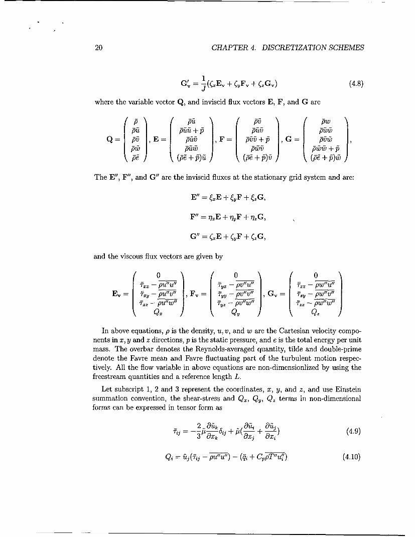
In above equations, p is the density, u, v, and w are the Cartesian velocity compo-nents in x, y and z directions, p is the static pressure, and e is the total energy per unitmass. The overbar denotes the Reynolds-averaged quantity, tilde and double-primedenote the Favre mean and Favre fluctuating part of the turbulent motion respec-tively. All the flow variable in above equations are non-dimensionlized by using thefreestream quantities and a reference length L.
Let subscript 1, 2 and 3 represent the coordinates, x, y, and z, and use Einsteinsummation convention, the shear-stress and Qx, Qy, Q, terms in non-dimensionalforms can be expressed in tensor form as
= 2 afti. ai-L aft49j = --- A---6•., + j4-x + (4.9)3 &Xk 1x x
Q= i2 (Nrij - p-,uT,"),-o+C P "u' (4.10)

4.2. TIME MARCHING SCHEME 21
where the mean molecular heat flux is
__ __ a2
l-Y )Prx (4.11)
The molecular viscosity i(T) is determined by Sutherland law, and a =
-i'yRT, is the speed of sound. The equation of state closes the system,
fie ( 1 1 2 P(U + 52 + V 2) + k (4.12)
where -y is the ratio of specific heats, k is the Favre mass-averaged turbulence kineticenergy. The turbulent shear stresses and heat flux appeared in above equations arecalculated by Baldwin-Lomax model[48]. The viscosity is composed of y + pt, wherept is the molecular viscosity and it is the turbulent viscosity determined by BaldwinLomax model. For a laminar flow, the pt is set to be zero.
4.2 Time Marching Scheme
The time dependent governing equation (4.1) is solved using the control volumemethod with the concept of dual time stepping suggested by Jameson [49]. A pseudotemporal term - is added to the governing equation (4.1). This term vanishes atthe end of each physical time step, and has no influence on the accuracy of the solu-tion. However, instead of using the explicit scheme as in [49], an implicit pseudo timemarching scheme using line Gauss-Seidel iteration is employed to achieve high CPUefficiency. For unsteady time accurate computations, the temporal term is discretizedimplicitly using a three point, backward differencing as the following
OQ 3Qn+l - 4Qn + Qn-i (4.13)
& = 2At
Where n is the time level index. The pseudo temporal term is discretized withfirst order Euler scheme. Let m stand for the iteration index within a physical timestep, the semi-discretized governing equation (4.1) can be expressed as
1 1.5 -R ,)+1,m]6Qn+1m+1 - R,+l,m 3Qf+lm - 4Q' + Q (- 1[(-A--r + Y-t)I-- (•-a) ' S- - 2At _(4.14)
where the Ai- is the pseudo time step, R is the net flux going through the controlvolume,

22 CHAPTER 4. DISCRETIZATION SCHEMES
-=[ e E R I+ (F'- -I • F )j + (G' - 1 G)k]ds (4.15)
where V is the volume of the control volume, s is the control volume surface area vec-tor. Equation (4.14) is solved using the unfactored line Gauss-Seidel iteration. Twoline sweeps in each pseudo time steps are used, one sweeps forward and the othersweeps backward. The alternative sweep directions are beneficial to the informationpropagation to reach high convergence rate. Within each physical time step, the so-lution marches in pseudo time until converged. The method is unconditionally stableand can reach very large pseudo time step since no factorization error is introduced.
4.3 The Zha E-CUSP Scheme[I, 2]
To clearly describe the formulations, the vectors Q and E' in Eq. (4.1) are givenbelow:
Q- pi) E'= -E, E a-- fti+± I (4.16)
PE Pz13LT+ p )
(U is the contravariant velocity in 6 direction and is defined as the following:
U == 6t + 6i + 6-yý + 6v (4.17)
U is defined as:
U = 0 - 6t (4.18)
The Jacobian matrix A is defined as:
a- -AT-' (4.19)
where T is the right eigenvector matrix of A, and A is the eigenvalue matrix of A onthe moving grid system with the eigenvalues of:
(U + C, U - C, U, U, U) (4.20)

4.3. THE ZHA E-CUSP SCHEME[?, ?1 23
where C is the speed of sound corresponding to the contravariant velocity:
C=cj + 2 + Q (4.21)
and where c = i-yRT is the physical speed of sound.
Due to the homogeneous relationship between Q and E, the following formulationapplies:
k = AQ = tki-1Q (4.22)
In an E-CUSP scheme, the eigenvalue matrix is split as the following:
( -C 00 00 00 000 i00 000 0 0 00 0 & =U[I]+ 0 0 0 0 0 (4.23)0 0 o0 0 0 0 oooo00 0 0 0 0+0 o o o o 0
The grid velocity term ýt[I] due to the moving mesh is naturally included in theconvective term, U, as given in Eq. (4.43). Therefore, Eq. (4.22) becomes:
(- 00o000 0 0 0 0E = TO[I]+ 0 0 0 0 0 }T-'Q= c+EP
0 0 0 0 0
pi(i + cyp5 (4.24)
where &c and &p are namely the convective and pressure fluxes. As shown above,the way of splitting the total flux into convective and pressure fluxes in an E-CUSPscheme is purely based on the analysis of characteristics of the system. As shown inEq. (4.24), the convective flux has the upwind characteristic 0 and is only associatedwith the convective velocity. The pressure flux has a downwind and an upwindcharacteristic and it completely depends on the propagation of an acoustic wave.

24 CHAPTER 4. DISCRETIZATION SCHEMES
The Zha E-CUSP2 scheme is based on the E-CUSP scheme suggested by Zha andHu [1], which is extended to a moving mesh system by the following:
E,• = }[()i (qWL + q°R) - IPUI 1 (q'R - q'L)] +2 2 2
0 0\
P+gi Y + P-P v (4.25)
2 2P(U2P(UC) + CO L
where
= (RLUI• + pRUj) (4.26)2
q =(4.27)
=1 (CL + OR) (4.28)2 2U3=2(L + R)
-MUL - UR (4.29)ML• = MR =c
2 2
OuI{M L+IMLI + 1[,(L +1)2 ML + IMLI (4.30)
2 + ]}4 24.0
UF = C' MR2 - '!RI + aR[--1(MýIR -1)2 _ MR- IMR2 (4.31)2 24 2
eL (P/P)L + (1///)R' LR = @P/P)L + (Pb/P)R (4.32)
1- 3 4.33
P= 1(M ± 1)2(2 T M) + cM(M2 - 1)2 = (4.33)
(4.34)

4.3. THE ZHA E-CUSP SCHEME[?, ?] 25
1(= -(L OR) (4.35)2 2
Please note that, in the energy equation of the pressure splitting, U and C areused instead of & and C. The term C is constructed by taking into account the effectof the grid velocity so that the flux will transit from subsonic to supersonic smoothly.When • = 0, Eq. (4.25) naturally returns to the one for a stationary grid.
For supersonic flow, when UL > C, Ei = EL; when UR < -C, Ei = ER.2 2
4.3.1 Numerical Dissipation
The low numerical dissipation at stagnation is important to accurately resolve wallboundary layers. An upwind scheme can be written as a central differencing plus anumerical dissipation.
To analyze the numerical dissipation at stagnation, the 1D Euler equation is usedas the example. Assuming u = 0, the numerical dissipation vector of the new E-CUSPscheme at stagnation is:
aiD 2 0o (4.36)
where
6P PR - PL (4.37)
The numerical dissipation of the Roe scheme at stagnation is:
/'(-y-_1)#i26p
DRoe =6- J) 0p (4.38)
where the-stands for the Roe's average[50].
Comparing eq.(4.36) and (4.38), it can be seen that the numerical dissipation ofthe new E-CUSP scheme for the continuity equation vanishes at u = 0 while the Roescheme has the non-vanishing dissipation. For the energy equation, the two schemeshave equivalent dissipation. For ideal gas with the -y = 1.4, the coefficient of theRoe scheme energy dissipation term is 2.5 times larger than that of the new E-CUSPscheme.
In conclusion, even though there is one non-vanishing numerical dissipation termin the energy equation for the new E-CUSP scheme, the overall numerical dissipation
26 CHAPTER 4. DISCRETIZATION SCHEMES
of the new E-CUSP scheme is not greater than that of the Roe scheme. The Roescheme is proved to be accurate to resolve wall boundary layers[51]. It is henceexpected that the new E-CUSP scheme should also have sufficiently low dissipationto accurately resolve wall boundary layers. This is indeed the case shown by thenumerical experiment for a flat plate boundary layer.
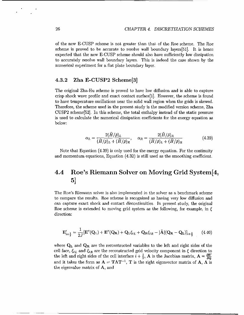
4.3.2 Zha E-CUSP2 Scheme[3]
The original Zha-Hu scheme is proved to have low diffusion and is able to capturecrisp shock wave profile and exact contact surface[l]. However, the scheme is foundto have temperature oscillations near the solid wall region when the grids is skewed.Therefore, the scheme used in the present study is the modified version scheme, ZhaCUSP2 scheme[52]. In this scheme, the total enthalpy instead of the static pressureis used to calculate the numerical dissipation coefficients for the energy equation asbelow:
= ~2(H/P)L 2(H/P)R
(H/I)L + (H/P)R' (H/p)L + (Hl/)R(
Note that Equation (4.39) is only used for the energy equation. For the continuityand momentum equations, Equation (4.32) is still used as the smoothing coefficient.
4.4 Roe's Riemann Solver on Moving Grid System[4,
5]
The Roe's Riemann solver is also implemented in the solver as a benchmark schemeto compare the results. Roe scheme is recognized as having very low diffusion andcan capture exact shock and contact discontinuities. In present study, the originalRoe scheme is extended to moving grid system as the following, for example, in •direction:
1
E/ I½= I-[E"(QL) + E"(QR) + QL&,L + QR&tR - I-AI(QR - QL)li+½ (4.40)it 2J 2
where QL and QR are the reconstructed variables to the left and right sides of thecell face, CtL and &tR are the reconstructed grid velocity component in ý direction tothe left and right sides of the cell interface i + ½, A is the Jacobian matrix, A = OE'
and it takes the form as A = TAT-1 , T is the right eigenvector matrix of A, A isthe eigenvalue matrix of A, and
4.5. CONVENTIONAL BOUNDARY CONDITIONS 27
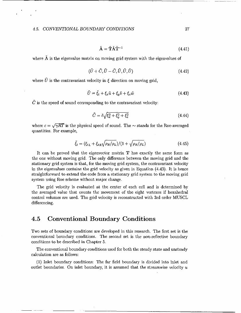
A = TAT-1 (4.41)
where A is the eigenvalue matrix on moving grid system with the eigenvalues of
(U +C,U-C,UU,U) (4.42)
where U is the contravariant velocity in ý direction on moving grid,
U"= + ý'ýi + 6j + ýIzv (4.43)
Sis the speed of sound corresponding to the contravariant velocity:
E =a + 6 + 2 (4.44)
where c = Vý7RT is the physical speed of sound. The r-' stands for the Roe-averagedquantities. For example,
6 = (6L + 6 PR/PL)/(1 + PR/-PL) (4.45)
It can be proved that the eigenvector matrix T has exactly the same form asthe one without moving grid. The only difference between the moving grid and thestationary grid system is that, for the moving grid system, the contravariant velocityin the eigenvalues contains the grid velocity as given in Equation (4.43). It is hencestraightforward to extend the code from a stationary grid system to the moving gridsystem using Roe scheme without major change.
The grid velocity is evaluated at the center of each cell and is determined bythe averaged value that counts the movement of the eight vertexes if hexahedralcontrol volumes are used. The grid velocity is reconstructed with 3rd order MUSCLdifferencing.
4.5 Conventional Boundary Conditions
Two sets of boundary conditions are developed in this research. The first set is theconventional boundary conditions. The second set is the non-reflective boundaryconditions to be described in Chapter 5.
The conventional boundary conditions used for both the steady state and unsteadycalculation are as follows:
(1) Inlet boundary conditions: The far field boundary is divided into inlet andoutlet boundaries. On inlet boundary, it is assumed that the streamwise velocity u

28 CHAPTER 4. DISCRETIZATION SCHEMES
is uniform, transverse velocity v = 0, and spanwise velocity w = 0. Other primitivevariables are specified according to the freestream condition except the pressure whichis extrapolated from interior.
(2) Outlet boundary conditions: All the flow quantities are extrapolated frominterior except the pressure which is set to be its freestream value.
(3) Solid wall boundary conditions: At moving boundary surface, the no-slip con-dition is enforced by extrapolating the velocity between the phantom and interiorcells,
u0 = 2b - U1, v 0 = 2 Yb - v1, w= 2ib - W1 (4.46)
where u0, v0 and w0 denote the velocity at phantom cell, ul, v, and w, denote thevelocity at the 1st interior cell close to the boundary, and Ub, Vb and wb are the velocityon the moving boundary.
If the wall surface is in 71 direction, the other two conditions to be imposed onthe solid wall are the adiabatic wall condition and the inviscid normal momentumequation[30] as follows,
T = 0, -+ (4.47)
4.6 Moving/Deforming Grid Systems
In the fully-coupled computation, the remeshing is performed in each iteration. There-fore, a CPU time efficient algebraic grid deformation method is employed in the com-putation instead of the commonly-used grid generation method in which the Poissonequation is solved for grid points. For clarity, the remeshing procedure for 2D cases issketched in Figure 12.131. This grid deformation procedure is designed in such a waythat the far-field boundary (j=jlp) is held fixed, and the grids on the wing surface(j=l) moves and deforms following the instantaneous motion of the wing structure.After the new wing surface is determined, two components of the displacement vectorat wing surface node dxj and dy1 can be calculated accordingly. First, the length ofeach segment along the old mesh line is estimated as:
s8 = s 3 -I + Vi(xj - xj- 1 )2 + (yj - yj,-) 2 (j = 2,. ,jlp) (4.48)
where s, = 0 and the displacement vectors at wing surface node ( dxl, dy1 ) and atthe far-field boundary ( dxjlp, dyjlp ) are known. Then the grid node points betweenthe wing surface and the far-field boundary can be obtained by using following linearinterpolation:
4.7. GEOMETRIC CONSERVATION LAW 29
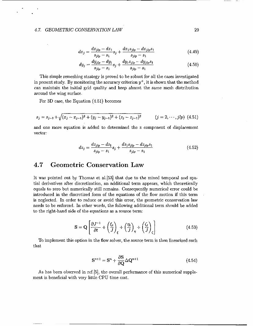
dxj dxjlp - dxl dxlsjlp - dxjlps, (4.49)sjup -- Si Sjlp - Si
dyj dyjlp - dy + dyisjlp - dyjps, (4.50)Sjip - Si sj1p - Si
This simple remeshing strategy is proved to be robust for all the cases investigatedin present study. By monitoring the accuracy criterion y+, it is shown that the methodcan maintain the initial grid quality and keep almost the same mesh distributionaround the wing surface.
For 3D case, the Equation (4.51) becomes
8j = sj-1 + V/(xj - xj-l)2 +t (yj - yj-l)2 +U (zj - zj-l), (j = 2, . jlp) (4.51)
and one more equation is added to determined the z component of displacementvector:
dzj = dzjp - dz + dzlslP - dzlps, (4.52)sjlp - s + Sjip - si
4.7 Geometric Conservation Law
It was pointed out by Thomas et al. [53] that due to the mixed temporal and spa-tial derivatives after discretization, an additional term appears, which theoreticallyequals to zero but numerically still remains. Consequently numerical error could beintroduced in the discretized form of the equations of the flow motion if this termis neglected. In order to reduce or avoid this error, the geometric conservation lawneeds to be enforced. In other words, the following additional term should be addedto the right-hand side of the equations as a source term:
S=Q aI- + 0- +1-1±1-lI (4.53)
To implement this option in the flow solver, the source term is then linearized suchthat
sn+ =S + a- L9 Q (4.54)
As has been observed in ref.[5], the overall performance of this numerical supple-ment is beneficial with very little CPU time cost.
30 CHAPTER 4. DISCRETIZATION SCHEMES

Chapter 5
Non-Reflective BoundaryConditions
5.1 Characteristic Form of the Navier-Stokes Equations[6]
The characteristic form of the Navier-Stokes equations in the generalized coordinateswill be solved to determine the non-reflective boundary conditions at the phantomcells. To describe the derivation process, the ý direction will be taken as an exam-ple. For the other two directions, the formulations can follow the same procedureand the general formulations are given in the appendix. Based on the strategy ofThompson[39] and Poinsot and Lele[33], the Navier-Stokes equations are expressedfirst using primitive variables as the following:
Oq aq Oq _qM- + A-M- + B -M•-7 + C M- = R, (5.1)
Tt 017 a(
where A, B, C are the Jacobian matrix
A E' = Of' OG' (5.2)A =- Bq" = -' C= (5--2)
where R, is the viscous vector on the right hand side of the Navier-Stokes equations,(Equation (4.1)), q is the primitive variable vector:
q = v (5.3)w
31

32 CHAPTER 5. NON-REFLECTIVE BOUNDARY CONDITIONS
M is the Jacobian matrix between the conservative variables and primitive variables
Mu 0 0 0
- i v 0 p 0 0 (5.4)q w 0 0 p 0
•-_ pu pv pw I -_
where cP 2 1 (U2 + V2 + w2).
Equation (5.1) can be further expressed as:
-&q + q a- & q c•-Oq9q+ + b--q + = M-Rv (5.5)
Where
a = M-1AM, b = M-1 BM, c = M- 1CM (5.6)
(1 0 0 0 010 0 0
-1 0 0 (5.7)_ 1-W 0 0 0ý, -u(-1) -v(y-1) -w(y- 1) - 1
Matrix a, b, c have the same eigenvalues as Jacobian matrix A, B, C. In • direction,
U PX. PG~, Pz 00 U 0 0 C-
a t0 0 U 0 f (5.8)0 0 0 U e
0 'p(X 'yPG 7PGz U
where U = Cu + ýyv + ý.w. Matrix a can also be expressed as
a = PAP` (5.9)
where A is the eigenvalue matrix, P is eigenvector matrix of a, and P` is the inverseof P. They are given as the following

5.1. CHARACTERISTIC FORM OF THE NAVIER-STOKES EQUATIONS[?] 33
( 0U 0 0 00 U 0 0 0
A 0 0 U 0 0 (5.10)0 0 0 U+C 00 0 0 0 U-C
P= 2& 0 - V2, -2VI/2 (5.11)-2,, & 0 ý./2--&/v/-0 0 0 ac, acC2
0 -•ii -&/c2
0 & -•d•P-1= -& 0 -&/C 2 (5.12)
0 /v2- /y / P0 -&1V2- -ýyIV2 -&1V2- 6
where C cIV6l, IV61 = + / -//, ,= Iv, z = +z/IV l,a = p/"'2/c, 63 = 1/V2pc, c is the speed of sound and determined by c -- 'yRT.
The Navier-Stokes equation, Equation (5.5) then can be expressed as:
T ~ a77 a(-t-+q PAP l + ba-•q +cL•= Mal (5.13)
orP-1q q pMb•1 O
+ AP-1 + P-lb+__ + P-'c- = P-1M-1p (5.14)
This is the characteristic form of the Navier-Stokes equations in C direction. Definevector £ as:
L = AP-Oq (5.15)
The Navier-Stokes equations (Equation (5.14)) are then expressed as:
P-9 +C + P- + P--cl- = P-'M-'Rv (5.16)
Vector £ is given as the following:
34 CHAPTER 5. NON-REFLECTIVE BOUNDARY CONDITIONS
+ G(•) + Um -4A
( L i5 ~ Z 5 ( )+ý5 ~ J -ý ia ý C 0 L a 5
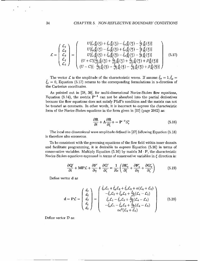
I= L3 U[A (-)+ •y•, )-L )- -C2 (5.17)
L4 (U + C)[1 (R) + + LL ()](u- c) [_- _L (u) - &Y_ - (.K - -L. L (- + -(P]
The vector L is the amplitude of the characteristic waves. If assume = 1, •= 0, Equation (5.17) returns to the corresponding formulations in x-direction of
the Cartesian coordinates.
As pointed out in [38, 39], for multi-dimensional Navier-Stokes flow equations,Equation (5.14), the matrix P`- can not be absorbed into the partial derivativesbecause the flow equations does not satisfy Pfaff's condition and the matrix can notbe treated as constants. In other words, it is incorrect to express the characteristicform of the Navier-Stokes equations in the form given in [37] (page 2042) as:
OR OR -_aR + A- -+= P S* (5.18)
The local one-dimensional wave amplitude defined in [37] following Equation (5.18)is therefore also erroneous.
To be consistent with the governing equations of the flow field within inner domainand facilitate programming, it is desirable to express Equation (5.16) in terms ofconservative variables. Multiply Equation (5.16) by matrix M. P, the characteristicNavier-Stokes equations expressed in terms of conservative variables in • direction is:
1Q' OF' OG' 1 ( OGMv a (5.19)-- •+ MP +-0-- + 0 e• 9 -+ -57- ,+09t o9( & Re\\O 0+a(j±(5.19)
Define vector d as
(d1 (CLj + ý,yL 2 + U3_ + Qe(L 4 + L5)d2 -&L2 + ý,L3 + (L- L5)
d=PL= 4ds = j +) (5.20)P d4 1 -6y - fx£3 + -_2(L4 + L5)
Deinvcc (to + as)
Define vector D) as:
5.2. NON-REFLECTIVE BOUNDARY CONDITIONS[?] 35
ud1 + pd2
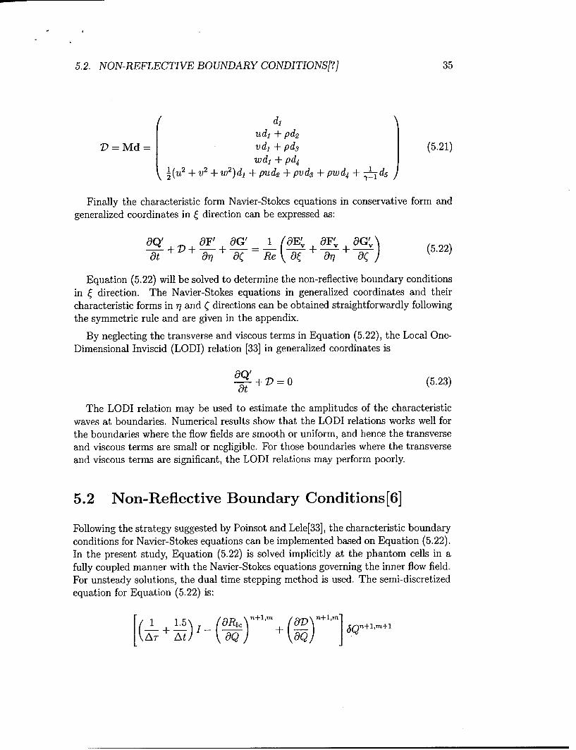
D=Md= vd, + pd 3 (5.21)wd1 + pd4I U2 +V2 +w2)d, pud2 +pvd3 pwd4 d
Finally the characteristic form Navier-Stokes equations in conservative form andgeneralized coordinates in ý direction can be expressed as:
OQ' 9F' WG' 1 (EM OF'v OG (5.22)+-- D + -+ + + + W F ]c)(.2Ot O19 'q Re a6 O ~
Equation (5.22) will be solved to determine the non-reflective boundary conditionsin 6 direction. The Navier-Stokes equations in generalized coordinates and theircharacteristic forms in r and ( directions can be obtained straightforwardly followingthe symmetric rule and are given in the appendix.
By neglecting the transverse and viscous terms in Equation (5.22), the Local One-Dimensional Inviscid (LODI) relation [33] in generalized coordinates is
0Q'9 + = 0 (5.23)
The LODI relation may be used to estimate the amplitudes of the characteristicwaves at boundaries. Numerical results show that the LODI relations works well forthe boundaries where the flow fields are smooth or uniform, and hence the transverseand viscous terms are small or negligible. For those boundaries where the transverseand viscous terms are significant, the LODI relations may perform poorly.
5.2 Non-Reflective Boundary Conditions[6]
Following the strategy suggested by Poinsot and Lele[33], the characteristic boundaryconditions for Navier-Stokes equations can be implemented based on Equation (5.22).In the present study, Equation (5.22) is solved implicitly at the phantom cells in afully coupled manner with the Navier-Stokes equations governing the inner flow field.For unsteady solutions, the dual time stepping method is used. The semi-discretizedequation for Equation (5.22) is:
[(1 + •.5) (aRb) n+I,m + (c•D• n+1m]j Qn+lm+l
36 CHAPTER 5. NON-REFLECTIVE BOUNDARY CONDITIONS
n+l, 3Qln+lm - 4Qn + Qn-1
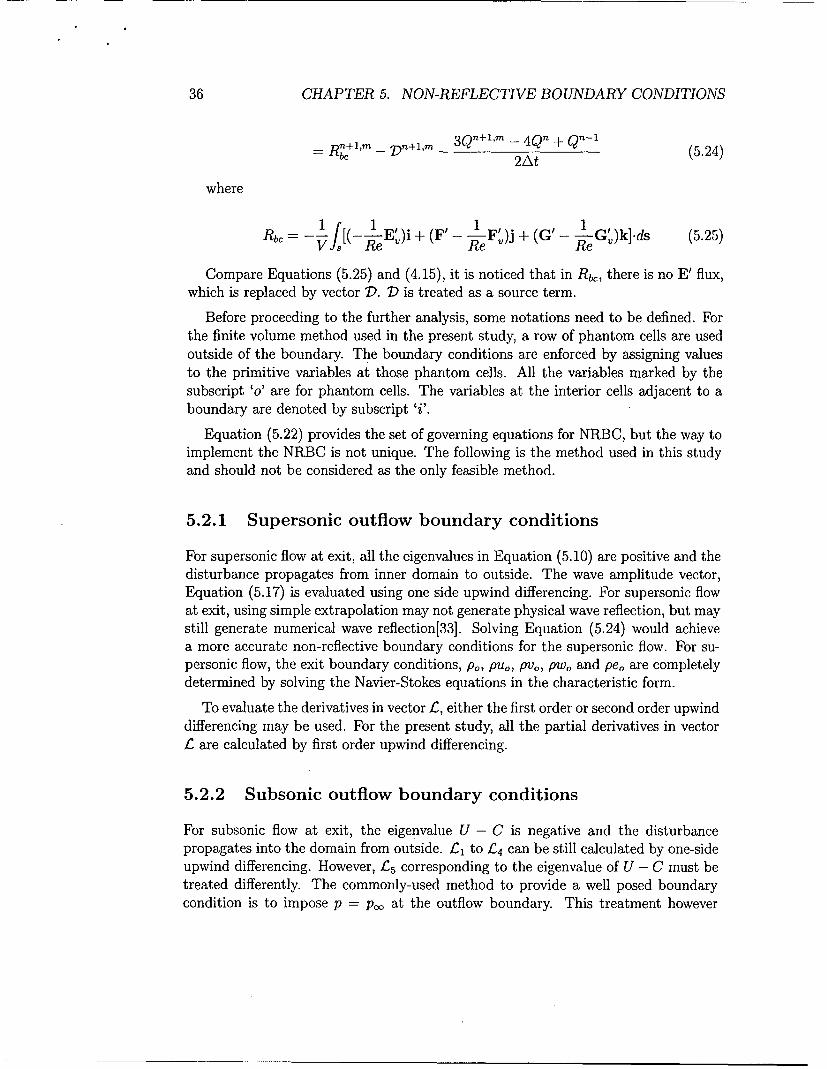
Dn+lm 2At (5.24)
where
Rb -) + (F' - 1 F')j + (G' - G')k]-ds (5.25)V Re Re W
Compare Equations (5.25) and (4.15), it is noticed that in Rb,, there is no E' flux,which is replaced by vector D. D is treated as a source term.
Before proceeding to the further analysis, some notations need to be defined. Forthe finite volume method used in the present study, a row of phantom cells are usedoutside of the boundary. The boundary conditions are enforced by assigning valuesto the primitive variables at those phantom cells. All the variables marked by thesubscript 'o' are for phantom cells. The variables at the interior cells adjacent to aboundary are denoted by subscript 'i'.
Equation (5.22) provides the set of governing equations for NRBC, but the way toimplement the NRBC is not unique. The following is the method used in this studyand should not be considered as the only feasible method.
5.2.1 Supersonic outflow boundary conditions
For supersonic flow at exit, all the eigenvalues in Equation (5.10) are positive and thedisturbance propagates from inner domain to outside. The wave amplitude vector,Equation (5.17) is evaluated using one side upwind differencing. For supersonic flowat exit, using simple extrapolation may not generate physical wave reflection, but maystill generate numerical wave reflection[33]. Solving Equation (5.24) would achievea more accurate non-reflective boundary conditions for the supersonic flow. For su-personic flow, the exit boundary conditions, po, pUo, pVo, pwo and peo are completelydetermined by solving the Navier-Stokes equations in the characteristic form.
To evaluate the derivatives in vector L, either the first order or second order upwinddifferencing may be used. For the present study, all the partial derivatives in vector£ are calculated by first order upwind differencing.
5.2.2 Subsonic outflow boundary conditions
For subsonic flow at exit, the eigenvalue U - C is negative and the disturbancepropagates into the domain from outside. £1 to C4 can be still calculated by one-sideupwind differencing. However, L5 corresponding to the eigenvalue of U - C must betreated differently. The commonly-used method to provide a well posed boundarycondition is to impose p = poo at the outflow boundary. This treatment however

5.2. NON-REFLECTIVE BOUNDARY CONDITIONS[?] 37
will create acoustic wave reflections, which may be diffused and eventually disappearwhen the solution is converged to a steady state solution. For unsteady flows, thewave reflection may contaminate the flow solutions. To avoid wave reflections, thefollowing soft boundary condition was suggested by Rudy-Strikwerda[54] and used byPoinsot-Lele[33].
£ 5 = K(P Pe) (5.26)
where KI is a constant and is determined by I oa(1-.AM2)c/L as given by Poinsot andLele in [33] for Cartesian coordinates. The corresponding form used in the generalizedcoordinates is
r = ,1l - M 2.I/(Vf2JpL) (5.27)
where M is the maximum Mach number in the flow field. L is the characteristiclength of the domain. c is the speed of sound. The preferred range for constant a is0.2-0.5. The absolute value of 1 - M 2 is to ensure the term is positive because themaximum Mach number can be greater than 1 in a transonic flow field.
If £5 = 0, it switches to the "perfect" non-reflective boundary condition. However,this boundary condition is not well posed and will not lead the solution to the onematching the exit pressure p,. Equation (5.26) assumes that the constant exit pres-sure p(, is imposed at infinity. There exists reflection if p / p,, which is needed forthe well posedness of the numerical solution. For the unsteady problems, Equation(5.26) will make the mean value of the pressure at the exit very close to p,,. However,the pressure at the individual control volume may not be exactly equal to p,) eventhough the value of L5 can be very small. In this sense, Equation (5.26) may beconsidered as "almost non-reflective boundary conditions".
The complete boundary conditions used at the exit are the pressure at infinity forEquation (5.26) and three zero gradient viscous conditions:
6 + c + Gr2y) = 0 (5.28)
(6Tr 2 + 6 + G7-.)= 0 (5.29)
-(6Q. + Wy + GzQ) = 0 (5.30)
The amplitudes of the outgoing characteristic waves, £L, £2, £3, and £4 are com-puted from the interior domain. All the conservative variables at phantom points are

38 CHAPTER 5. NON-REFLECTIVE BOUNDARY CONDITIONS
obtained by solving the characteristic N-S equations, Equation (5.22). All the trans-verse and viscous terms in Equation (5.22) can be evaluated in the same way as theinner domain control volumes. The Roe's Riemann solver is also used for computingfluxes F' and G', central differencing is used for fluxes E,, F•, F•. This strategymakes maximum use of the existing code and minimizes the programming work inimplementing the boundary conditions.
5.2.3 Subsonic inflow boundary conditions
At C = 1 boundary, four characteristic waves, L1, £2, £3, and £4 are entering thedomain while £5 is leaving the domain. For 3-D open field flow cases, four physi-cal boundary conditions are needed, i.e. uo, vo, wo and po are set to be constant.Other primitive variables are specified according to the freestream condition. Thetotal energy peo is obtained by solving the energy equation in Equation (5.22). Theoutgoing wave £5 can be estimated by using interior variables. The rest of the wavesare evaluated by using the LODI relations, Equation (5.23). £L - £4 can be expressedas
Li " (£4±£5), L2=-y "' (£4-i- 5), L3=4.~ P (£4±£s), £4=£,5
(5.31)
5.2.4 Adiabatic wall boundary conditions
At a 3-D adiabatic wall (77 = constant), the no-slip condition is enforced by extrapo-lating the velocity between the phantom and interior cells, u. = -ui, vo = -vi, andw, = -wi. One more physical boundary condition to be imposed on the wall is theadiabatic condition, 2' = 0. From the adiabatic condition, the Po can be expressed871as the following
Po = A (5.32)Po Pi
The total energy peo is determined by solving the energy equation in Equation(5.22). Then using Equation (5.32) and Equation (??), Po and po can be solved.Cross a r/boundary, vector £ is expressed as the following:

5.2. NON-REFLECTIVE BOUNDARY CONDITIONS[?] 39
I allV[(a)) + - 4- 8 - o]
I2 1 Y-(2-)1 (L )+i J ~ - 7 kJV-3 -V ' (5.33)14(V + C)[•-?/ a(R) + _9 + . + 8ofE +
(V5 C " V a• ' J v/2- J J N52 a7 lJ - 77) J
where V = 77.u + 77yV +7, rw and C = clVl, lV?7 = 2 + 2 + q It can be seen
from Equation (5.33), the characteristic waves £L - L3 vanish since V = 0 at wallsurface. At lower wall (r7 = 1), the outgoing characteristic wave L5 is computed fromthe interior domain. The incoming wave £4 is estimated by using LODI relations.By solving 2nd - 4th equations in Equation (5.23), it yields £4 = £5. At upper wall(maximum ii), the £4 becomes the outgoing wave, and it can be computed from theinterior domain. £C is the incoming wave which is evaluated by £f = £4.
40 CHAPTER 5. NON-REFLECTIVE BOUNDARY CONDITIONS
Chapter 6
Structural Models
6.1 Modal Approach for 3D Wing[4]
The governing equation of the solid structure motion can be written as,
Md2 + Cd +Ku=f (6.1)dWt2 dt
where M, C and K are the mass, damping, and stiffness matrices of the solid respec-tively, u is the displacement vector and f is the force exerted on the surface nodepoints of the solid, both can be expressed as:
U- ui ,f= fi ,
U, f,
where N is the total number of node points of the structural model, ui and fi arevectors with 3 components in x, y, z directions:
ui= uiy j, f= f2• •.Uiz fiy
Ui 2 , f/ fi~
fi is dynamic force exerted on the surface of the solid body. In a modal approach,the modal decomposition of the structure motion can be expressed as follows:
41
42 CHAPTER 6. STRUCTURAL MODELS
K(b = M4A (6.2)
or
KO., = A3M¢j (6.3)
where A is eigenvalue matrix, A diag[Al,-..., A•,, , A3N], and jth eigenvalue Aj -
W, , yj is the natural frequency of jth mode, and the mode shape matrix 4)
Equation (6.15) can be solved by using a finite element solver (e.g. ANSYS) toobtain its finite number of mode shapes Oj. The first five mode shapes will be usedin this paper to calculate the displacement of the structure such that,
u(t) = X aj(t)oj = I)a (6.4)
where a = [a,, a2 , a3 , a 4 , a 5 ]T. Substitute Equation (6.4) to Equation (6.1) and yield
M)(d2a C da)dt2 dt
Multiply Equation (6.5) by 4 )T and re-write it as
l +iad2a (6da)dt 2 dt
where P-- [P1,P 2,- ., .P, ,PN]T, the modal force of jth mode, P3 = c'f, themodal mass matrix is defined as
S= 4TMI) = diag(m,.. ,-- 3,... ,m3N) (6.7)
where mj is the modal mass of jth mode, and the modal damping matrix is definedas
ITC4 = diag(cl,. .. , ,.. ., C3N) (6.8)
where cj is the modal damping of jth mode, and the modal stiffness matrix is definedas
]k = 4T K(b = diag(k,.. -,ki,... ,k3g) (6.9)

6.1. MODAL APPROACH FOR 3D WING[?] 43
where kj is the modal stiffness of jth mode. Equation (6.6) implies
d2 aj dai 2 (.10dt2 + 2(jwj- f + a, (610)
where (j is modal damping ratio. Equation (6.18) is the modal equation of struc-ture motion, and is solved numerically within each iteration. By carefully choosingreference quantities, the normalized equation may be expressed as
d 2a + 2~ (j +j = ;T .V. (bf ) -- (6.11)dt.* 2( w, -d---+ • W a v*
where the dimensionless quantities are denoted by an asterisk, W, is the naturalfrequency in pitch, b, is the streamwise semichord measured at wing root, L is thereference length, fin is the measured wing panel mass, v* is the volume of a conicalfrustum having streamwise root chord as lower base diameter, streamwise tip chord asupper base diameter, and panel span as height, V* = u-o and U.. is the freestream
velocity.
Then the equations are transformed to a state form and expressed as:
als}[M] ý + [K]{S} = q (6.12)
where
aj ,M [I],K= (Eý_•2 2 - 'q= )h2•-- j 2(OjTf*V* (_I fin
To couple the structural equations with the equations of flow motion and solve themimplicitly in each physical time step, above equations are discretized and integratedin a manner consistent with Equation (4.14) to yield
(1 1+ +K) 6Sn+lm+l -M3Sn -4Sn + S-I - KS'•+",m + qn+lm+l
(6.13)
where n is the physical time level index while m stands for the pseudo time index.The detailed coupling procedure between the fluid and structural systems is given inthe following chapter.

44 CHAPTER 6. STRUCTURAL MODELS
6.2 Mistuned Bladed Structural Model for Tran-sient Response
The Subsets of Nominal Modes (SNM) structural model suggested by Yang and Grif-fin [43] is developed in this research for time domain to calculate the structural modes,which are expensive to calculate if the direct finite element approach is used. Yangand Griffin recognized that each mistuned structural mode can be well representedby a subset of the tuned structural modes. The SNM approach was developed totake the finite element modal solution of the tuned structure as the input to formu-late a reduced order model for the mistuned structure. The order of the problemthus dropped from millions to hundreds, and the computational time to compute amistuned structural mode is reduced from hours to seconds. This is critical to thesimulation of fully coupled fluid-structural problems because only very limited com-putational resource is required in addition to the CPU intensive CFD computation.A brief description of the SNM model is in the following:
a) Transformation from Finite Element Domain to Modal Domain
First, the equation of motion in the finite element form is transformed into themodal coordinates. Assuming that the variation of the mechanical damping is negli-gible, then
(M! + A!M)& + &°& + (ko + Ak)a = p (6.14)
In eq. (6.14), the modal coordinate vector a is the displacements of the tunedmodes, AM0 , C&, and k 0 are the modal mass, damping, and stiffness matrices of thetuned system, and typically diagonal, AK and AM are the changes in modal stiffnessand mass matrices, and p is the modal force vector. Eq. (6.14) can then be cast in astate space form,
BS, = Ay + q (6.15)
where
B ( 0 y Ao) (6.16)( 0 (]0) +0 A 6A= (•0+A!) -_o 0 q- (p 6.7
Eq. (6.15) is the modal equation of motion for the mistuned structure. Withouttruncating the modes, the order of eq. (6.15) is 2N where N is the number of degrees offreedom of the whole wheel finite element model. However, the order can be reduced
6.2. MISTUNED BLADED STRUCTURAL MODEL FOR TRANSIENT RESPONSE45
to 2n, where n is tuned modes selected in the SNM representation, to simulate themistuned structural vibration with sufficient accuracy. N (millions) is typically muchgreater than n (hundreds).
b) Diagonalization of the Modal Governing Equation
To improve the computational efficiency, the solution of eq. (6.15) can be furtherexpressed in terms of its right eigenvectors R which satisfies the following eigenvalueproblem
AR= BRA (6.18)
where A is the diagonal eigenvalue matrix of the mistuned structure. Applying theclassical modal analysis technique, eq. (6.15) can be transformed in a diagonal form
BP = A,3 + 4l (6.19)
where the diagonal matrices b and A are the generalized mass and stiffness ma-trices, 3 is the generalized coordinates, and q is the generalized forces. Since thecomponents of 3 are decoupled from each other, eq. (6.19) can be simulated at verylow computational costs.
Note that, in eq. (6.19), b and A mathematically define a mistuned bladed diskstructure, the generalized force t is derived from the pressure distribution on theairfoil surfaces, and the time-varying unknown 3 will be solved at each time step.
46 CHAPTER 6. STRUCTURAL MODELS

Chapter 7
Fully Coupled Fluid-StructuralInteraction
To rigorously simulate fluid-structural interactions, the equations of flow motion andstructural response need to be solved simultaneously within each iteration in a fullycoupled numerical model. The calculation based on fully coupled iteration is CPUexpensive, especially for three dimensional applications. The modal approach cansave CPU time significantly by solving the modal displacement equations, Eq. (6.18),instead of the original structural equations, Eq. (6.15), which is usually solved byusing finite element method. In the modal approach, the structural mode shapescan be pre-determined by using a separate finite element structural solver. Oncethe several mode shapes of interest are obtained, the physical displacements can becalculated just by solving those simplified linear equations, i.e., Eqs. (6.18) and(6.4). In present study, the first five mode shapes provided in Ref.[55] are usedto model the wing structure. These pre-calculated mode shapes are obtained on afixed structural grid system and are transformed to the CFD grid system by using a3rd order polynomial fitting procedure. The procedure is only performed once andthen the mode shapes for CFD grid system are stored in the code throughout thesimulation.
The procedure of the fully coupled fluid-structure interaction by modal approachis described below:
(1) The flow solver provides dynamic forces on solid surfaces.
(2) Integrate fluid forces at each surface element to obtain the forcing vector f.
(3) Use Eq. (6.18) to calculate modal displacements aj(j = 1, 2, 3, 4, 5) of the nextpseudo time step.
(4) Use Eq. (6.4) to calculate physical displacement u of the next pseudo timestep.
47

48 CHAPTER 7. FULLY COUPLED FLUID-STRUCTURAL INTERACTION
(5) Check the maximum residuals of both solutions of the flow and the structuralequations. If the maximum residuals are greater than the prescribed convergencecriteria, go back to step (1) and proceed to the next pseudo time. Otherwise thecalculation of the flow field and the structural displacement within the physical timestep is completed and the next new physical time step starts. The procedure is alsoillustrated in the flow chart given in Fig. 12.132.
Initial flow field and structuralsolutions, Q", S"
Aerodynamic forces
-II
Cy Structural displacerment , iby solving structural _. ,,
U) equations sn+l.ml J0. 0.
CFD moving and deformingmesh u)
E EI�0
CFD flow field by solvingflow governing equations •,IL-Sa.~l ,m~l IL.J
Xz
No CFD and structural Yes
Figure 7.1: Fully coupled flow-structure interaction procedure
Chapter 8
Results and Discussion
8.1 Validation of Zha-Hu E-CUSP Schemes[I]
The original Zhu-Hu E-CUSP scheme described from Eq. 4.25 to 4.35 was developedand then used as the basis for the Zha E-CUSP2 scheme.
8.1.1 Shock Tubes
For shock tube problems, the interests are focused on: 1) the quality (monotonicityand sharpness) of the shock and contact discontinuities; 2)the maximum allowableCFL number to be used for explicit Euler method.
For explicit Euler time marching scheme, it is desirable that the CFL number isclose to the upper limit of 1.0. For the 1D linear wave equation with CFL=I and 1storder upwind scheme, the numerical dissipation and dispersion vanish. For nonlinearEuler equations, it is also true that the closer the CFL to 1.0, the less the numericaldissipation.
The Sod Problem
Fig. 12.1 to 12.5 are the computed temperature distributions using different upwindschemes with first order accuracy compared with the analytical result of the Sodproblem[56]. Since the computation stops before the waves reach either end of theshock tube, the first order extrapolation boundary conditions are used at both endsof the shock tube for all the schemes.
The maximum allowable CFL number for a scheme is defined as: beyond whichthe solution will either be oscillatory or unstable. The new E-CUSP scheme (ZhaCUSP in the figures) achieves maximum CFL of 1.00, and the shock profile is the
49

50 CHAPTER 8. RESULTS AND DISCUSSION
crispest and remains monotone (Fig.12.1). The maximum allowable CFL of Roe andVan Leer scheme are 0.95 and 0.96 respectively. The new E-CUSP scheme takes threegrid points across the shock wave, while the Roe and Van Leer schemes take four gridpoints (see Fig.12.1, 12.2 and 12.3). The Van Leer scheme generates a tail at the endof the expansion wave (see Fig. 12.3). Interestingly, the Van Leer-HlInel scheme canreach maximum CFL =1.0 and the shock profile is also crisper than the original VanLeer scheme with no tail generated at the end of the expansion wave (see Fig. 12.4).All the schemes smear the contact surface to a similar extent. The expansion waveis captured well by all the schemes. The AUSM+ scheme has the unexpectedly lowmaximum allowable CFL of 0.275. The whole shock and contact surface profiles areseriously smeared due to the low maximum CFL number.
The table 8.1 given below summarizes the maximum allowable CFL number foreach scheme. Overall, for the Sod 1D shock tube problem, the new scheme suggestedin this paper performs the best based on the shock sharpness, monotonicity, andstability.
Table 8.1: Maximum CFL Numbers for Sod 1D Shock Tube
Scheme CFL NumberThe new scheme (Zha CUSP) 1.00Van Leer-Hldnel 1.00Van Leer 0.96Roe 0.95Liou AUSM+ 0.275
Slowly Moving Contact Surface
This is a shock tube case used in [57] to demonstrate the capability of the scheme tocapture the contact surface. The initial conditions are [p, u,p]L = [0.125, 0.112, 1.0],[p, u,p]R = [10.0, 0.112, 1.0] . All the results are first order accuracy. Fig. 12.6 showsthat the new E-CUSP scheme, the Roe scheme and the AUSM+ scheme all can resolvethe contact surface accurately as they are designed. The results of those schemes areat time level 0.01. The velocity is uniformly constant and the density discontinuity ismonotone. The new E-CUSP (Zha CUSP) scheme has far higher CFL number thanthe other schemes with the value of 1.00. The Roe scheme has the max CFL=0.3,and Liou's MUMS+ has 0.48. Fig.12.7 shows that the Roe scheme generates largevelocity oscillations when CFL=0.35, greater than its max CFL=0.3.
The schemes of Van Leer, Van Leer-HInel severely distort the profiles of the contactsurfaces as shown in Fig. 12.8. The velocity profiles are largely oscillatory. Thedensity jumps are also more smeared.

8.1. VALIDATION OF ZHA-HU E-CUSP SCHEMES[?] 51
The table 8.2 lists the maximum CFL number of each scheme for the slowingmoving contact surface. Again, the new scheme outperforms the other schemes byhaving the highest CFL number and still maintain the monotonicity.
Table 8.2: Maximum CFL numbers of the schemes resolving the contact surface
Scheme CFL NumberThe new E-CUSP (Zha CUSP) scheme 1.00Liou AUSM+ 0.48Roe 0.32Van Leer failVan Leer-Hinel fail
8.1.2 Entropy condition
This case is to test if a scheme violates the entropy condition by allowing the expansionshocks. The test case is a simple quasi-ID converging-diverging transonic nozzle[58,59]. The correct solution should be a smooth flow from subsonic to supersonic with noshock. However, for an upwind scheme which does not satisfy the entropy condition,an expansion shock may be produced.
For the subsonic boundary conditions at the entrance, the velocity is extrapolatedfrom the inner domain and the other variables are determined by the total temper-ature and total pressure. For supersonic exit boundary conditions, all the variablesare extrapolated from inside of the nozzle. The analytical solution was used as theinitial flow field. Explicit Euler time marching scheme was used to seek the steadystate solutions. All the schemes use first order differencing.
Fig. 12.9 is the comparison of the analytical and computed Mach number distribu-tions with 201 mesh points using the new scheme and the scheme of Roe, Van Leer,Van Leer-Hdnel, Liou's AUSM+. The analytical solution is smooth throughout thenozzle and reaches the sonic speed at the throat (the minimum area of the nozzle,located at X/h = 4.22). It is seen that both the Roe scheme and Van Leer schemegenerate a strong expansion shock at the nozzle throat. Both schemes can convergeto machine zero (12 order of magnitude) with CFL=0.95 even with the expansionshock waves.
The Van Leer-Hdnel scheme can not converge even with CFL=0.01. The resultplotted in Fig. 12.9 is the one before it diverges. It shows an expansion shock withthe Mach number jumping from 0.74 to 1.42. The AUSM+ also has difficulties toconverge for this case. Using CFL=0.05, it managed to reduce the residual by 4 orderof magnitude. The solution of the AUSM+ also shows an expansion shock with the

52 CHAPTER 8. RESULTS AND DISCUSSION
Mach number jumping from 0.86 to 1.17.
The new E-CUSP scheme does not have an expansion shock wave at the sonic point,but is not smooth due to the discontinuity of the first derivative of the pressure at thesonic point. This is shown as a small glitch at the sonic point in fig. 12.9. The glitchdoes not affect the scheme to converge the solution to machine zero with CFL=0.95.
As indicated in [58, 59], the amplitude of the expansion shock decreases when themesh is refined. When the 2nd order schemes with the MUSCL differencing are used,all the expansion shock waves as well as the glitch of the new scheme at the sonicpoint disappear. Since this paper is to compare the original Riemann solver schemes,no entropy fix[60] that can remove the expansion shock of Roe schemes was used.
8.1.3 Wall Boundary Layer
To examine the numerical dissipation of the new scheme, a laminar supersonic bound-ary layer on an adiabatic flat plate is calculated using first order accuracy. The in-coming Mach number is 2.0. The Reynolds number based on the length of the flatplate is 40000. The Prandtl number of 1.0 is used in order to compare the numer-ical solutions with the analytical solution. The baseline mesh size is 81x61 in thedirection along the plate and normal to the plate respectively.
Fig. 12. 10 is the comparison between the computed velocity profiles and the Blasiussolution. The solutions of the new scheme (Zha CUSP), Roe scheme, and AUSM+scheme agree very well with the analytical solution. The Van Leer scheme significantlythickens the boundary layer. The Van Leer- Hdnel scheme does not improve thevelocity profile.
Fig.12.11 is the comparison between the computed temperature profiles and theBlasius solution. Again, the new scheme (Zha CUSP), Roe scheme, and AUSM+scheme accurately predict the temperature profiles and the computed solutions ba-sically go through the analytical solution. Both the Van Leer scheme and the VanLeer- Hdnel scheme significantly thicken the thermal boundary layer similarly to thevelocity profiles.
Table 8.3 shows the wall temperature predicted by all the schemes using the base-line mesh and refined mesh. The predicted temperature value by the Van Leer schemehas a large error. The Van Leer- Hdnel scheme does predict the wall temperatureaccurately even though the overall profile is nearly as poor as that predicted by theVan Leer scheme. The new scheme, Roe scheme and AUSM+ scheme all predict thetemperature accurately.
All the results mentioned above are converged based on mesh size. The walltemperatures using the refined mesh of 161 x 121 are also given in table 8.3. There islittle difference between the results of the baseline mesh and the refined mesh. Therefined mesh does not help to reduce the large numerical dissipation of the Van Leer

8.1. VALIDATION OF ZHA-HU E-CUSP SCHEMES[?] 53
scheme. When the 2nd order schemes are used, both the velocity and temperatureprofiles of the Van Leer scheme and Van Leer- Hdnel are improved (not shown).
Scheme T,,a11 , Mesh 80 x 60 Twa11, Mesh 160 x 120Blasius analytical solution 1.8000 1.8000
The new E-CUSP (Zha CUSP) scheme 1.8025 1.8018Roe scheme 1.8002 1.7996
Liou AUSM+ 1.8000 1.8000Van Leer 1.8328 1.8333
Van Leer-Hiinel 1.7970 1.7996
Table 8.3: Computed non-dimensional wall temperature using first order schemeswith the baseline mesh and refined mesh
8.1.4 Transonic Converging-Diverging Nozzle
To examine the performance of the new scheme in two-dimensional flow and thecapability to capture the shock waves which do not align with the mesh lines, atransonic converging-diverging nozzle is calculated as inviscid flow. The nozzle wasdesigned and tested at NASA and was named as Nozzle A1[61]. Third order accuracyof MUSCL type differencing is used to evaluate the inviscid flux with the Minmodlimiter. Fig.12.12 is the computed Mach number contour using the new E-CUSPscheme with the mesh size of 175 x 80. In the axial direction, there are 140 meshpoints distributed downstream of the nozzle throat, where the oblique shock wavesare located. The grid is clustered near the wall. For clarity, the coarsened mesh isdrawn as the background with the Mach contours to show the relative orientation ofthe shock waves and the mesh lines. The nozzle is symmetric about the centerline.Hence only upper half of the nozzle is calculated. The upper boundary uses theslip wall boundary conditions and the lower boundary of the center line uses thesymmetric boundary conditions.
As indicated by the wall surface isentropic Mach number distribution shown infig.12.13, the flow is subsonic at the inlet with the Mach number about 0.22 and isaccelerated to sonic at the throat, and then reaches supersonic with Mach numberabout 1.35 at the exit. Fig.12.12 shows that right after throat, an expansion fanemanates from the wall and accelerates the flow to reach the peak Mach numberabout 1.5. Due to the sharp throat turning, an oblique shock appears immediatelydownstream of the expansion fan to turn the flow to axial direction. The two obliqueshocks intersect at the centerline, go through each other, hit the wall on the otherside, and then reflect from the wall. Such shock patten is repeated to the exit andthe shock strength is weakened with the flow going downstream. Fig. 12.13 showsthat the isentropic Mach number distributions predicted by the new CUSP scheme
54 CHAPTER 8. RESULTS AND DISCUSSION
and the Roe scheme agree fairly well with the experiment. The new E-CUSP schemeand the Roe scheme have virtually indistinguishable results.
The mesh refinement study indicates that the mesh resolution in the axial directiondoes not affect the shock resolution much. The axial mesh size of 280 downstream ofthe throat yields only slightly better shock resolution than the size of 70. However,the mesh size in the vertical direction dramatically changes the shock resolution. Theniesh size of 80 in the vertical direction yields much better resolution than the meshsize of 50. This can be seen from the isentropic Mach number in fig.12.13, whichshows that the mesh size of 175 x 80 generates much sharper profiles than those ofthe mesh 175x 50 for the first and second shock reflections.
For this transonic nozzle with the mesh size 175 x 80 on an Intel Xeon 1.7Ghzprocessor, the CPU time per time step per node to calculate the inviscid flux is2.5871 x 10's for the new scheme, which is about 25% of the CPU time of 1.0284 x10's used for the Roe scheme. This is a significant CPU time reduction.
8.1.5 Transonic Inlet-Diffuser
To examine the performance of the new scheme for shock wave/turbulent boundarylayer interaction, a transonic inlet-diffuser[62] is calculated as shown by the Machnumber contours in fig.12.14, which has the exit back pressure equal to 0.83 times ofthe inlet total pressure. The Reynolds number based on the throat height is 4.38 x 101.The Baldwin-Lomax[48] algebraic turbulence model is used. Third order accuracy ofMUSCL-type differencing with the Minmod limiter is used for the inviscid fluxes andthe second order central differencing is used for the viscous terms.
A normal shock is located downstream of the throat as shown in fig.12.14. No flowseparation is generated under this back pressure. The baseline mesh size is 100 x 60.When y+ is held as constant and the mesh is refined in both the horizontal andvertical direction, the results have little variation and are converged based on meshsize. All the inlet-diffuser results presented in this paper are from the mesh size of100 x 120. The mesh in the horizontal direction is clustered around the shock locationto better resolve the shock profile.
Fig. 12.15 is the comparison of the upper wall surface pressure between the experi-ment and the computation. The agreement is very good except that the computationpredicts the shock location a little downstream of the experimental shock location andthe shock strength a little too strong. It is found that the shock profile is sensitiveto the y'. The y' value of 2,2 x 10-, 7 x 10⁻⁶ are tested. The smaller y' yieldsa little closer shock location to the experiment. The results shown in fig.12.14 and12.15 have the y' value of 2 x 10'. The small y' effect is believed due to the firstorder extrapolation of the pressure on wall surface instead of the requirement of theturbulence modeling. In the region with no shock, the first order pressure extrapola-
8.2. VALIDATION OF THE ZHA E-CUSP2 SCHEME[?] 55
tion on the wall is insensitive to the distance of the first cell to the wall, while in theshock region it is sensitive due to the large streamwise gradient. As indicated in fig.12.15, the Roe scheme predicts the shock location slightly closer to the experimentthan the new CUSP scheme.
When the back pressure is reduced to 0.72 times of the inlet total pressure. Thenormal shock is stronger and the flow separation is induced. The same mesh as theprevious case is used for this case. Fig.12.17 is the predicted pressure distributioncompared with the experiment. Both the new CUSP scheme and the Roe schemepredict the shock location accurately, but the shock strength predicted is too strong.However, the new scheme has the pressure profile in the separation region downstreamof the shock noticeably closer to the experiment than that predicted by the Roescheme.
It should be pointed out that the turbulence modeling is a critical factor for theprediction accuracy of the shock wave/turbulent boundary layer interaction. Hencethe discrepancy between the calculation and experiment shown above is only partiallyattributed to the different discretization schemes.
Fig.12.17 is the pressure contours computed using pot/pt = 0.72 with the newscheme, Roe Scheme, and Liou's AUSM+ scheme. A curved A shock is formed dueto the shock wave/turbulent boundary layer interaction. The shape of the Machcontours of the new scheme (Zha CUSP) and the Roe scheme are very much alike.The contours computed by the AUSM+ scheme has significant oscillations near thewall.
8.2 Validation of the Zha E-CUSP2 Scheme[3]
The Zha E-CUSP2 scheme defined from Eq. 4.25 to 4.39 was validated for the shocktube and laminar boundary layer. The results are as good as the original Zha-Huscheme or better. More importantly, the Zha E-CUSP2 scheme has cured the tem-perature oscillation of the original Zha-Hu scheme as shown below.
8.2.1 Transonic Converging-Diverging Nozzle
To examine the performance of the new scheme in two-dimensional flow and thecapability to capture the shock waves which do not align with the mesh lines, atransonic converging-diverging nozzle is calculated as inviscid flow. The nozzle wasdesigned and tested at NASA and was named as Nozzle A1[61]. Third order accuracyof MUSCL type differencing is used to evaluate the inviscid flux with no limiter.
Fig.12.18 is the computed Mach number contours using the original Zha CUSPscheme and the Zha CUSP2 scheme with the mesh size of 175 x 80. The nozzle is
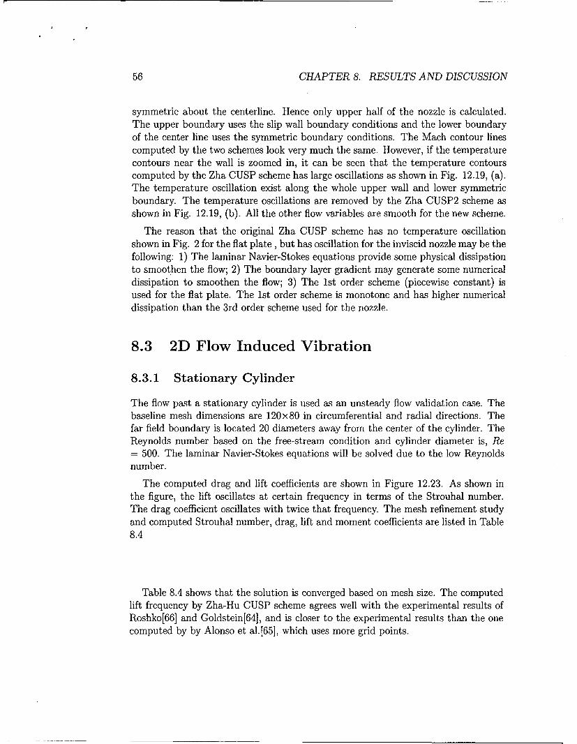
56 CHAPTER 8. RESULTS AND DISCUSSION
symmetric about the centerline. Hence only upper half of the nozzle is calculated.The upper boundary uses the slip wall boundary conditions and the lower boundaryof the center line uses the symmetric boundary conditions. The Mach contour linescomputed by the two schemes look very much the same. However, if the temperaturecontours near the wall is zoomed in, it can be seen that the temperature contourscomputed by the Zha CUSP scheme has large oscillations as shown in Fig. 12.19, (a).The temperature oscillation exist along the whole upper wall and lower symmetricboundary. The temperature oscillations are removed by the Zha CUSP2 scheme asshown in Fig. 12.19, (b). All the other flow variables are smooth for the new scheme.
The reason that the original Zha CUSP scheme has no temperature oscillationshown in Fig. 2 for the flat plate, but has oscillation for the inviscid nozzle may be thefollowing: 1) The laminar Navier-Stokes equations provide some physical dissipationto smoothen the flow; 2) The boundary layer gradient may generate some numericaldissipation to smoothen the flow; 3) The 1st order scheme (piecewise constant) isused for the flat plate. The 1st order scheme is monotone and has higher numericaldissipation than the 3rd order scheme used for the nozzle.
8.3 2D Flow Induced Vibration
8.3.1 Stationary Cylinder
The flow past a stationary cylinder is used as an unsteady flow validation case. Thebaseline mesh dimensions are 120x80 in circumferential and radial directions. Thefar field boundary is located 20 diameters away from the center of the cylinder. TheReynolds number based on the free-stream condition and cylinder diameter is, Re= 500. The laminar Navier-Stokes equations will be solved due to the low Reynoldsnumber.
The computed drag and lift coefficients are shown in Figure 12.23. As shown inthe figure, the lift oscillates at certain frequency in terms of the Strouhal number.The drag coefficient oscillates with twice that frequency. The mesh refinement studyand computed Strouhal number, drag, lift and moment coefficients are listed in Table8.4
Table 8.4 shows that the solution is converged based on mesh size. The computedlift frequency by Zha-Hu CUSP scheme agrees well with the experimental results ofRoshko[66] and Goldstein[64], and is closer to the experimental results than the onecomputed by by Alonso et al.[65], which uses more grid points.
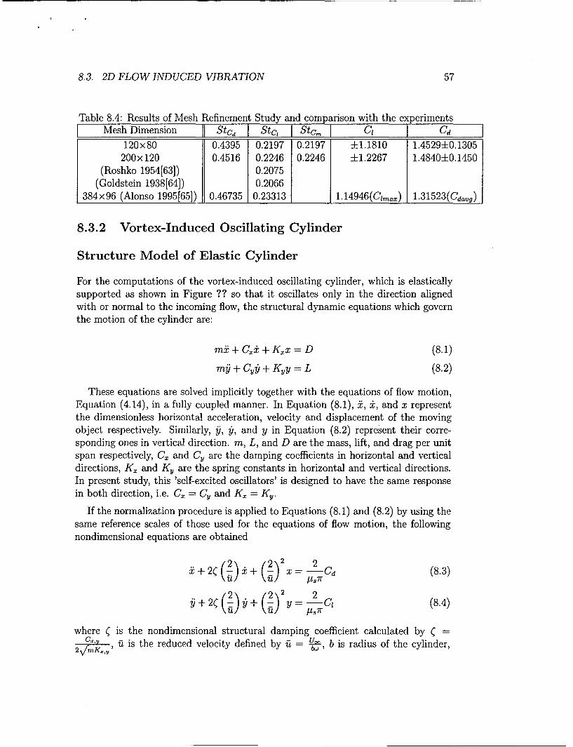
8.3. 2D FLOW INDUCED VIBRATION 57
Table 8.4: Results of Mesh Refinement Study and comparison with the experimentsMesh Dimension Stcd I Stc, I Stcm T CL Cd
120x80 0.4395 0.2197 0.2197 ±1.1810 1.4529±0.1305200x120 0.4516 0.2246 0.2246 ±1.2267 1.4840±0.1450
(Roshko 1954[63]) 0.2075(Goldstein 1938[64]) 0.2066
384x96 (Alonso 1995[65]) 0.46735 0.23313 1.14946(Cimax) 1.315 23(Cdavg)
8.3.2 Vortex-Induced Oscillating Cylinder
Structure Model of Elastic Cylinder
For the computations of the vortex-induced oscillating cylinder, which is elasticallysupported as shown in Figure ?? so that it oscillates only in the direction alignedwith or normal to the incoming flow, the structural dynamic equations which governthe motion of the cylinder are:
m: + CQx +K~xD (8.1)
mij + CQ + Kyy = L (8.2)
These equations are solved implicitly together with the equations of flow motion,Equation (4.14), in a fully coupled manner. In Equation (8.1), ,, ±, and x representthe dimensionless horizontal acceleration, velocity and displacement of the movingobject respectively. Similarly, ji, y, and y in Equation (8.2) represent their corre-sponding ones in vertical direction. m, L, and D are the mass, lift, and drag per unitspan respectively, C. and Cy are the damping coefficients in horizontal and verticaldirections, Kx and Ky are the spring constants in horizontal and vertical directions.In present study, this 'self-excited oscillators' is designed to have the same responsein both direction, i.e. Cx = Cy and K. = Ky.
If the normalization procedure is applied to Equations (8.1) and (8.2) by using thesame reference scales of those used for the equations of flow motion, the followingnondimensional equations are obtained
!i + 2( (1 + (2)X = 2-Cd (8.3)
9+ 2 (2 + (2 ) = 2 C (8.4)
where • is the nondimensional structural damping coefficient calculated by • =2 mx ,i is the reduced velocity defined by Ui= -, b is radius of the cylinder,

58 CHAPTER 8. RESULTS AND DISCUSSION
w = m, the mass ratio, ps Cd and Cp are the drag and lift forcecoefficients respectively. Then the equations are transformed to a matrix form andexpressed by
[M]--• + [K]{S} = q (8.5)
where X 0 -1 0 0 00S=() M =2[I]K(=2 0 0r -Cd
y Y ' [11, K 0 0 0 -1 q 0(1)2 2~(Q) p
To couple the structural equations with the equations of flow motion and solve themimplicitly in each physical time step, above equations are discretized and integratedin a manner consistent with Equation (4.14) to yield
(1-1 + 1'5 M + K) 6S+m+l = -M 3Sn+lm -2At4Sn + S-1 -KSn+lm + qn+lm+l
(8.6)
where n is the physical time level index while m stands for the pseudo time index.The detailed coupling procedure between the fluid and structural systems is given insection 4.
After validating the stationary cylinder vortex shedding flow, the cylinder is re-leased to be controlled by the structure model as shown in Figure ??. The corre-sponding structural equations are given in section 3.1. The laminar Navier-Stokesequations are solved due to the low Reynolds number, Re = 500.
Using the temporally periodic solution obtained in the computation of stationarycylinder as the initial flow field, the computation is resumed after the cylinder is letto move in both streamwise and transverse directions. For the purpose of comparisonwith the experimental data of Griffin[67] several different combinations of structuralparameters are used in the computations.
Morton et al.[30] suggested to use the reduced velocity f t such that thestructural oscillator works under or near the resonance conditions. Therefore thecomputed St number from the stationary cylinder is used to determine ia. For all thecases of oscillating cylinder, St is set to be 0.2, corresponding to ii = 1.5915. Differentmass ratios, p,, are used to test the different responses of the structural system. Theyare equal to 1.2732, 5.0, and 12.7324 respectively. To match the wide range of theexperimental data, the damping ratio, C, is chosen from the range between 0.001 -1.583.
8.3. 2D FLOW INDUCED VIBRATION 59
The dimensionless physical time step At = 0.05 is used, which corresponds toapproximately 100 time steps per period determined by the Strouhal number used.The CFL number for the pseudo time steps varies from case to case. For the largecylinder movement cases, smaller pseudo time steps are used to limit the displacementof the cylinder during each iteration.
For the cases computed, the CFL number varies from 5 to 500. The iterationnumber within one physical time step varies from 20 to 100. Fig. 12.24 shows atypical iteration history within one physical time step. Both the residual of theCFD solver and structure are reduced to machine zero. The structure solver usuallyconverges faster than the CFD solver.
Figure 12.25 displays the computed vorticity contours around the oscillating cylin-der. It shows how the vortexes are shed at the moment when the cylinder boundsback toward its mean position in y direction.
A typical trajectory of the center position of the moving cylinder is plotted inFigure 12.26, which is similar to the results computed by Blackburn et al.[68] andAlonso et al.[65]
All the numerical results for present study are plotted in Figure 12.27 for the threevalues of p,. Also plotted are the computations of Alonso et al. [65] with p. =
5.0, computations of Morton et al.[30] with p =' 12.73, and the experimental dataof Griffin[67]. In the figure, the abscissa is the reduced damping with the form of87r2St2(_- [68], and the ordinate is the cross-flow displacement of motion normalizedby the diameter of the cylinder. Overall, very good agreement is observed betweenthe present results and the experimental results, especially for the case of p, = 1.2732.The figure shows that the higher values of mass ratios (L = 5.0 and IL = 12.7324)give less satisfactory results than those with I, -- 1.2732, particularly at low dampingratios. However, they agree well with the results of Morton et al.[30] (/t, = 12.73).
8.3.3 Elastically Mounted Airfoil
As the validation of the Zha-Hu CUSP scheme for transonic airfoils, the steady statesolution of the transonic RAE 2822 airfoil is calculated first. The freestream conditionfor this study are listed in Table 8.5 below.
Table 8.5: Free-stream condition for RAE 2822 Airfoil
Mach number Static Pressure (psia) Temperature (R) Angle-of-Attack (deg) Reynolds Number]
0.729 15.8073 460.0 2.31 6.5"x×10'

60 CHAPTER 8. RESULTS AND DISCUSSION
The turbulent Reynolds stress and heat flux is calculated by the Baldwin-Lomaxalgebraic model[48]. This case is run using an O-type grid with three different di-mensions, they are 128x50x1, 256x55x1, and 512x95xI respectively. The outerboundary extends to 15 chords from the center of the airfoil. The experimental dataprovided by Cook et al.[69] are available for validation. The comparison of pressurecoefficient on the airfoil is shown in Figure 12.28. Overall, very good agreement isobtained between the computation and experiment for each mesh dimension, espe-cially for the two larger ones which appear to be sufficient to capture the shock on thesuction surface of the airfoil without using any limiter. The important aerodynamiccoefficients from both simulation and experiment are summarized in Table 8.6.
Table 8.6: Aerodynamic coefficients and y+ for RAE 2822 AirfoilMesh Dimension Cd C, Cm Y+
128x50 0.01482 0.73991 0.09914 0.0833 - 2.3864256x55 0.01455 0.73729 0.09840 0.1318 - 2.4016512x95 0.01426 0.74791 0.09994 0.2309 - 2.0228
Prananta et al.[701 0.01500 0.74800 0.09800Experiment 0.01270 0.74300 0.09500
It can be seen in Table 8.6 that the predicted lift coefficients with all mesh dimensionsagree well with the experiment. The computed drag and moment coefficients showlarger errors, but they have the similar accuracy as those computed by Prananta etal.[70]. The relatively large error of the drag and moment may be mostly due to theinadequacy of the turbulence model, which is difficult to predict the surface frictionaccurately.
8.3.4 Forced Pitching Airfoil
As a validation case of the scheme for moving grid system, the forced pitching NACA64A010 airfoil is calculated. For this transonic airfoil, the Reynolds averaged Navier-Stokes equations with Baldwin-Lomax turbulence model are solved. Similar to theprevious computation of the flow over the stationary airfoil, an O-type mesh consistingof 280x65 cells is employed for the computations of forced pitching airfoil. TheNACA 64A0101 airfoil is selected for this calculation because the experimental datais available. The fine mesh zone or the non-deforming part of the mesh is shown inFigure 12.29. The first grid point adjacent to the wall has the maximum y+ < 3.43
The NACA 64A0101 airfoil is forced in pitch around its quarter chord sinusoidally.The angle of attack is imposed as a function of time as a(t) = am + aosin(wt), wheream and ao are the mean angle of attack and the amplitude of oscillation respectively.
8.3. 2D FLOW INDUCED VIBRATION 61
The w is the angular frequency which is directly related to the reduced frequencyK, 'c2-, where c is the airfoil chord, and U,, is the free-stream velocity. Tocompare with the experimental results given by Davis[71], the primary parametersused in the computation are listed as follows: am = 0, a, = 1.010, Re = 1.256 x 10⁷,Mm = 0.8, reduced frequency, K, = 0.202.
Again, the computation begins with the steady state flow field of the stationaryairfoil at 0 degree angle of attack with a dimensionless time step At = 0.1. Thetransition period takes about 3 cycles and the results becomes periodic in time afterthat. Figure 12.30 shows the lift oscillation versus the angle of attack after the flowfield reaches its temporally periodic solution. The computed lift oscillation agreeswell with the experiment[71], which has an evident improvement compared to therecent result computed by McMullen et al. in 2002 [72].
Fig. 12.31 shows the computed moment coefficient compared with the experiment[71].The computed moment coefficient does not agree as accurately with the experimentas the lift coefficient does. However the results are very similar to those predicted byBohbot et al. [73] and McMullen et al. [72]. The large discrepancy between the compu-tation and the experiment for the moment coefficient may be due to the inadequacyof the turbulence modeling, which may not predict the surface friction accurately.
8.3.5 Flow-Induced Vibration of NACA 64A010 Airfoil
Structural Models
The structural model for the flow-induced vibration of a 2-D sweptback wing with aNACA 64A010 cross-section is described in section. This model was first introducedby Isogai [74] [74], and has been numerically investigated by several researchers [10][75] [70] [73].
The system of the elastically mounted airfoil is assumed to be undamped. Theairfoil is allowed to move in pitch about a given elastic axis and plunge vertically. Thepitch axis is defined by a distance a, which is the multiple of the semi-chord lengthwith the origin point located at the mid-chord position. If a is positive, it means theaxis is located downstream of the mid-chord, negative means being located upstreamof the mid-chord point.
A sketch of the elastically mounted airfoil is depicted in Figure 12.21. The motionof such an elastic system can be described by using the following equations
mh + S,±& + Khh =-L (8.7)
Sh + d+ K = M (8.8)
where h and a are the plunging and pitching displacements respectively, m is the mass

62 CHAPTER 8. RESULTS AND DISCUSSION
per unit span, Sc, is the static moment around the elastic axis, I,, is the rotationalmoment of inertia, Kh and K& are plunging and pitching spring constants respectively,L is the lift force and M is the moment around the elastic axis. The equations of thestructure motion (8.7) and (8.8) are normalized by using semi-chord b as the lengthdimension, the uncoupled natural frequency in pitch w,' as the time scale, and areexpressed as
+h+xcd+ h=---C1 (8.9)
U2S C + + (8.10)a /tr
where x,, is the static unbalance, Wh is the uncoupled natural frequency in plunge, r2
is the squared radius of gyration, U* is the reduced velocity defined as U-, C1 and Cmare the lift and moment coefficient respectively. Since the time scale used in Equations(8.9) and (8.10) is different from the one used in the governing equations of flow, thestructural dimensionless time t* needs to be re-scaled and keep its consistency with theentire system during the computation, i.e., t* = &aLt*, where is the dimensionlesstime for flow and the L is the length scale. Finally the equations are cast into theform of Equations (8.5) and (8.6), and the corresponding matrices are
h 1 0 ' 0 0 0 -1 0001 2()2 - 7 U1~o.2Xc, 0 r 00 u.
The structural parameters used in this model are listed as the following: a = -2.0,xc, = 1.8, •h-=1, r•2 = 3.48, and JL = 60. The elastic axis is located half a chordupstream of the airfoil nose.
The unsteady Reynolds averaged Navier-Stokes equations with the Baldwin-Lomaxturbulence model are solved for the flow field in this study. The freestream conditionsare: Re = 1.256 x l0T, Mm = 0.825.
Due to the NACA 64A010 airfoil, an initial perturbation is
imposed to trigger the oscillating motion. The airfoil is forced to rotate sinusoidallyabout its elastic axis at the natural frequency in pitch wc, with an angle of attackamplitude, ao = 10. Usually the forced pitching mode lasts for 1 - 3 cycles. Afterthat, the elastically mounted airfoil is let to move in both plunging and pitchingdirections, and then the dynamic response is recorded.
In present study, the search of the critical point on the transonic flutter boundaryat a given Mach number is conducted. The speed index, V* defined as h is the
parameter to classify damped, neutral and divergent responses of the airfoil when theMach is fixed. In this case, the total pressure and temperature need to be adjusted
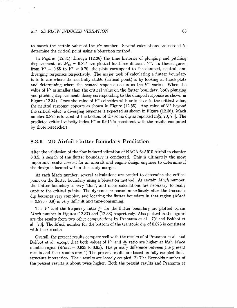
8.3. 2D FLOW INDUCED VIBRATION 63
to match the certain value of the Re number. Several calculations are needed todetermine the critical point using a bi-section method.
In Figures (12.34) through (12.36) the time histories of plunging and pitchingdisplacements at M, = 0.825 are plotted for three different V*. In these figures,from V* = 0.55 to V* = 0.70, the plots correspond to the damped, neutral, anddiverging responses respectively. The major task of calculating a flutter boundaryis to locate where the neutrally stable (critical point) is by looking at those plotsand determining where the neutral response occurs as the V* varies. When thevalue of V* is smaller than the critical value on the flutter boundary, both plungingand pitching displacements decay corresponding to the damped response as shown inFigure (12.34). Once the value of V* coincides with or is close to the critical value,the neutral response appears as shown in Figure (12.35). Any value of V* beyondthe critical value, a diverging response is expected as shown in Figure (12.36). Machnumber 0.825 is located at the bottom of the sonic dip as reported in[5, 70, 73]. Thepredicted critical velocity index V* = 0.615 is consistent with the results computedby those researchers.
8.3.6 2D Airfoil Flutter Boundary Prediction
After the validation of the flow induced vibration of NACA 64A010 Airfoil in chapter8.3.5, a search of the flutter boundary is conducted. This is ultimately the mostimportant results needed for an aircraft and engine design engineer to determine ifthe design is located within the safety margin.
At each Mach number, several calculations are needed to determine the criticalpoint on the flutter boundary using a bi-section method. At certain Mach number,the flutter boundary is very 'thin', and more calculations are necessary to reallycapture the critical points. The dynamic response immediately after the transonicdip becomes very complex, and locating the flutter boundary in that region (Mach= 0.875 - 0.9) is very difficult and time-consuming.
The V* and the frequency ratio - for the flutter boundary are plotted versusMach number in Figures (12.37) and (12.38) respectively. Also plotted in the figuresare the results from two other computations by Prananta et al. [70] and Bohbot etal. [73]. The Mach number for the bottom of the transonic dip of 0.825 is consistentwith their results.
Overall, the present results compare well with the results of of Prananta et al. andBohbot et al. except that both values of V* and -! ratio are higher at high Machnumber region (Mach = 0.925 to 0.95). The primary difference between the presentresults and their results are: 1) The present results are based on fully coupled fluid-structure interaction. Their results are loosely coupled; 2) The Reynolds number ofthe present results is about twice higher. Both the present results and Prananta et

64 CHAPTER 8. RESULTS AND DISCUSSION
al. are based on the same Baldwin-Lomax turbulence model. To study the effect ofReynolds number, the flutter boundary at Mach = 0.925 and 0.95 are re-calculatedwith the same Reynolds number (6 x 10⁶) used by Prananta et al. The difference issmall. Hence, the difference between the present results and the results of of Pranantaet al. and Bohbot et al. may be due to the fully coupled and loosely coupled algorithm.Since there are no experimental results for comparison, it is difficult to judge whichresult is more correct.
Except the flutter boundary, the present solver also has captured the Limit CycleOscillation (LCO) phenomenon as shown in Figure (12.39). LCO occurs when thevelocity index is greater than the flutter velocity index[76]. The amplitude is large,but stable. LCO is considered due to the nonlinear nature of the shock boundary layerinteraction occurring for transonic airfoil[76, 73]. Figure (12.40) presents a differentLCO with the second torsion mode more dominant.
Figure (12.41) shows an interesting situation happening at Mach = 0.875 andin the area of V* = 2.5. Both plunging and pitching displacements of the systemincrease rapidly immediately after the airfoil is set to be free, but then graduallyreach their steady state positions and stay there through the end of the computation.Under this flow condition, the aerodynamic forces and moments are balanced by thestructure system. The angle of attack is stabilized at 2.90 and is in the range of thecruise point which should be stable. This situation is only observed at Mach = 0.875,and maybe named as 'standing'. The V* of the standing phenomenon is not locatedat one point, but a region around V* = 2.5. The results and flow conditions of the'standing' phenomenon needs to be confirmed by experiment.
8.4 SNM Model Used for Transient Response
A structural model is developed to simulate the transient response of a blade diskstructure. This model implements the original SNM theory (for steady state re-sponses) and expands it to simulate transient responses. The study discussed in thissection assumes that the fluid forcing function is prescribed such that the transientresponse can be carried out in the transient simulation of ANSYS. The prescribedforcing function however does have multiple frequency components with all but oneprimary frequency components decaying in time.
Fig. 12.42 shows a finite element model of 24-blade disk with dynamic character-istics similar to a typical high compressor rotor. The finite element mesh is rathercoarse for the purpose of tractable computational cost in ANSYS benchmark com-putation. When studying a realistic case, the mesh needs to be finer. The transientresponses of this model were computed by two methods: In the first method, the tran-sient responses were calculated using the "Full Solution" function in ANSYS whichutilizes full system matrices (instead of reduced modal matrices in "Reduced Solu-
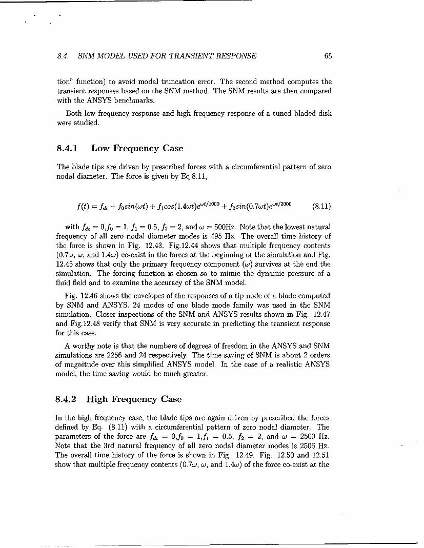
8.4. SNM MODEL USED FOR TRANSIENT RESPONSE 65
tion" function) to avoid modal truncation error. The second method computes thetransient responses based on the SNM method. The SNM results are then comparedwith the ANSYS benchmarks.
Both low frequency response and high frequency response of a tuned bladed diskwere studied.
8.4.1 Low Frequency Case
The blade tips are driven by prescribed forces with a circumferential pattern of zeronodal diameter. The force is given by Eq.8.11,
f(t) fd, + fosin(wt) + ficos(1.4wt)ewt/1 000 + f2sin(O.7wt)ewt/ 2000 (8.11)
with fd 0,fo = 1, f] = 0.5, f2 = 2, and w = 500Hz. Note that the lowest naturalfrequency of all zero nodal diameter modes is 495 Hz. The overall time history ofthe force is shown in Fig. 12.43. Fig.12.44 shows that multiple frequency contents(0.7w, w, and 1.4w) co-exist in the forces at the beginning of the simulation and Fig.12.45 shows that only the primary frequency component (w) survives at the end thesimulation. The forcing function is chosen so to mimic the dynamic pressure of afluid field and to examine the accuracy of the SNM model.
Fig. 12.46 shows the envelopes of the responses of a tip node of a blade computedby SNM and ANSYS. 24 modes of one blade mode family was used in the SNMsimulation. Closer inspections of the SNM and ANSYS results shown in Fig. 12.47and Fig.12.48 verify that SNM is very accurate in predicting the transient responsefor this case.
A worthy note is that the numbers of degrees of freedom in the ANSYS and SNMsimulations are 2256 and 24 respectively. The time saving of SNM is about 2 ordersof magnitude over this simplified ANSYS model. In the case of a realistic ANSYSmodel, the time saving would be much greater.
8.4.2 High Frequency Case
In the high frequency case, the blade tips are again driven by prescribed the forcesdefined by Eq. (8.11) with a circumferential pattern of zero nodal diameter. Theparameters of the force are fd 0,f0 o= 1j,f = 0.5, f2 = 2, and w = 2500 Hz.Note that the 3rd natural frequency of all zero nodal diameter modes is 2506 Hz.The overall time history of the force is shown in Fig. 12.49. Fig. 12.50 and 12.51show that multiple frequency contents (0.7w, w, and 1.4w) of the force co-exist at the

66 CHAPTER 8. RESULTS AND DISCUSSION
beginning of the simulation and only the primary frequency component (w) survivesat the end the simulation.
Fig. 12.52 compares the envelopes of the responses of a tip node of a blade com-puted by SNM and ANSYS. Only 24 modes of the 3rd blade mode family were usedin the SNM simulation. Fig. 12.53 and Fig. 12.54 are closer examination of theresponses. It is apparent that SNM does not capture the response well initially whenthe forcing frequency components and are yet to die out but does capture the re-sponse quite well at the end when the primary frequency component dominates. Thisis because of the lack of low and high frequency modes in the SNM model. In thiscase, the SNM model actually acts as a frequency filter of the overall system. Whenlong term steady state solution is of the only interest, an SNM model with a singleblade mode family might be desirable.
To further verify the above statement, an SNM model with the 3rd blade modefamily and the neighboring families (2nd and 4th blade modes) was used for thecomputation. Fig. 12.55, 12.56, and 12.57 compare the responses computed by SNMand ANSYS. They show good agreement between SNM and the ANSYS benchmark.Notice that the number of degrees of freedom in the 3-family SNM model is 72. Thetime saving of SNM is about 1.5 orders of magnitude over the ANSYS model.
8.5 Non-Reflective Boundary Conditions
8.5.1 A Vortex propagating through a outflow boundary
The first test case is a subsonic vortex propagating flow in an open flow field. Thecomputed domain is rectangular inclined 30' about the horizontal axis as a validationfor the generalized coordinates. The subsonic inflow and outflow boundary conditionsare used at the inlet and exit, and far filed boundaries are used on the upper and lowerborders. In [331, a supersonic vortex propagating flow is chosen. It is known that asubsonic vortex propagating flow is more difficult to deal with since the disturbancepropagates both upstream and downstream. To test present method under moregeneral conditions, the subsonic vortex propagating flow is selected for this study.
The computational mesh has a length of 2 units in streamwise direction which is30 degrees to the x direction, while the width is 4 units in transverse direction. Themesh dimensions are 60 x 100. The laminar Navier-Stokes equations is solved for thisflow with M = 0.8 and Reynolds number of 300.
A vorticity is initially located at the center of the domain when dimensionless timet* = 0, and convected downstream toward the outflow boundary. The velocity flowfield is initially specified as

8.5. NON-REFLECTIVE BOUNDARY CONDITIONS 67
U = u" 85+ (8.12)
C= cexp (X2 +v2 ) (8.13)
where u, and v, are the velocity components of the incoming flow, C, is the coef-
ficient that determines the vortex strength of the velocity field, and R, is the vortexradius. The total energy field is initialized as
pe =pe +pexp( 2 (8.14)
where C, is the coefficient that determines the vortex strength of the total energy field.Equations (8.12) and (8.14) are adopted from those used by Poinsot and Lele[33]. Thecoefficients C, and C,, and radius R, are defined by
C,,/(cL) =-0.0005, Ce/(cL) = -0.02, R, = 0.15 (8.15)
The inflow and outflow boundary conditions used in this case are described inprevious section. The far field upper and lower boundaries are treated as perfectnon-reflective outflow boundary.
The flow field at inflow boundary is initially set to be uniform. The direction of theincoming flow is parallel to the constant q7 lines. Obviously, at the inflow boundary,the transverse flux and viscous terms are very small. The error caused by LODIrelations is very small and negligible.
To compare the present NRBC with the commonly-used outflow boundary condi-tions (FPBC) in which the fixed downstream pressure is imposed for subsonic flowsimulations, the first computation is carried out with FPBC, which includes: at in-flow boundary, u,, vo, p, are given such that the streamwise velocity component isuniformly distributed and the transverse velocity component is equal to zero, thepressure is extrapolated from the interior domain, p. = pi, then the total energy peocan be computed from the equation of state; at outflow boundary, all the primitivevariables are extrapolated from the inner domain except the pressure is set to beconstant. The CFL number of the pseudo time step is 500. The physical time stepCFL is 0.74, which is determined by the time accuracy of the physical problem
The same case with the same initial flow condition and same CFL number is thencalculated using the NRBC developed in present study. The value of a in Equation(5.27) is set to be 0.25. Figures 12.58 and 12.59 show the computed density contours atfour instants by FPBC and NRBC respectively. It can be seen from figure 12.58 thatthe flow field is seriously distorted by the reflective waves when the vortex propagates
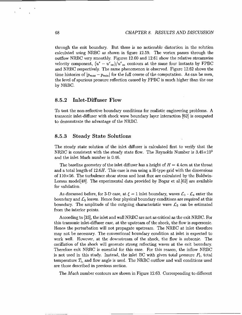
68 CHAPTER 8. RESULTS AND DISCUSSION
through the exit boundary. But there is no noticeable distortion in the solutioncalculated using NRBC as shown in figure 12.59. The vortex passes through theoutflow NRBC very smoothly. Figures 12.60 and 12.61 show the relative streamwisevelocity component, (u' - u T )/u'r contours at the same four instants by FPBCand NRBC respectively. The same phenomenon is observed. Figure 12.62 shows thetime histories of IPmaz - Pminl for the full course of the computation. As can be seen,the level of spurious pressure reflection caused by FPBC is much higher than the oneby NRBC.
8.5.2 Inlet-Diffuser Flow
To test the non-reflective boundary conditions for realistic engineering problems. Atransonic inlet-diffuser with shock wave boundary layer interaction [62] is computedto demonstrate the advantage of the NRBC.
8.5.3 Steady State Solutions
The steady state solution of the inlet diffuser is calculated first to verify that theNRBC is consistent with the steady state flow. The Reynolds Number is 3.45x10⁵
and the inlet Mach number is 0.46.
The baseline geometry of the inlet diffuser has a height of H = 4.4cm at the throatand a total length of 12.6H. This case is run using a H-type grid with the dimensionsof 110x56. The turbulence shear stress and heat flux are calculated by the Baldwin-Lomax model[48]. The experimental data provided by Bogar et al.[62] are availablefor validation.
As discussed before, for 3-D case, at • 1 inlet boundary, waves £l - L4 enter theboundary and L5 leaves. Hence four physical boundary conditions are required at thisboundary. The amplitude of the outgoing characteristic wave 45 can be estimatedfrom the interior points.
According to [33], the inlet and wall NRBC are not as critical as the exit NRBC. Forthis transonic inlet-diffuser case, at the upstream of the shock, the flow is supersonic.Hence the perturbation will not propagate upstream. The NRBC at inlet thereforemay not be necessary. The conventional boundary condition at inlet is expected towork well. However, at the downstream of the shock, the flow is subsonic. Theoscillation of the shock will generate strong reflecting waves at the exit boundary.Therefore exit NRBC is essential for this case. For this reason, the inflow NRBCis not used in this study. Instead, the inlet BC with given total pressure Pt, totaltemperature Tt, and flow angle is used. The NRBC outflow and wall conditions usedare those described in previous section.
The Mach number contours are shown in Figure 12.63. Corresponding to different

8.5. NON-REFLECTIVE BOUNDARY CONDITIONS 69
back pressure in the experiment, there are two cases of the flow, one has a weakshock (pouatet/pt=0.8 2) and the other has a strong shock (poutlet/pt=0. 72 ). Figures12.64 and 12.65 show the computed static pressure distributions compared with theexperimental data along the top and bottom wall for the weak shock case. Goodagreement is obtained between the computation and experiment.
Figures 12.66 and 12.67 show the static pressure distribution compared with theexperimental data along the top and bottom walls for the strong shock case. Dueto the strong shock interacting with the turbulent boundary layer, there is a flowseparation downstream of the shock, which is not well predicted. There may be tworeasons for the problem: 1) the flow is unsteady due to the separation and hencethe steady state solution can not capture the separation bubble length correctly; 2)the Baldwin-Lomax turbulence model is inadequate to handle the non-equilibriumseparated flow.
Different a values from 0.1 to 0.35 are tested and the results show that the steadystate results are insensitive to the a value. The fixed pressure boundary conditions arealso applied to the same case, and achieve almost the same results as those computedby the NRBC. This is because that, for the steady state solutions, the reflective wavesare eventually diffused when the steady state solution is converged.
8.5.4 Unsteady Solutions
The steady state calculation indicates that the NRBC is not essential since the ar-tificial reflective waves are diffused when the solution is converged. However, it isvery different when the unsteady flow is calculated. For the inlet-diffuser case with astrong shock wave, the fixed pressure outflow boundary conditions (FPBC) generatesstrong reflective waves and makes the shock wave severely oscillating inside the duct.The amplitude of the oscillation is far greater than the experimental results. Whenthe NRBC is applied, the shock oscillation is dramatically reduced.
Figures 12.68 and 12.69 show the time averaged pressure distributions comparedwith the experimental data. The CFL number of the pseudo time step is equal to 5for all the cases. The CFL number of the physical time step is about 3000, which gives132 steps in a shock oscillation cycle of the computed dominant frequency 260(Hz).The value of a in Equation (5.27) is 0.25. Due to the large shock oscillation, theshock location is smeared out for the fixed pressure outflow boundary conditions(FPBC). Hence the shock location, strength and the pressure downstream of theshock are poorly predicted. When the NRBC is applied, the reduced shock oscillationyields sharp shock profile and much better agreement of the shock location with theexperiment.
To match the experimental geometry for the measured shock oscillation frequency,the computational domain is then extend to a total length of 21.3H. The simulation

70 CHAPTER 8. RESULTS AND DISCUSSION
is carried out with FPBC and NRBC respectively using the same flow conditions.The computed and experimental power spectra for the static pressure at the exitlocation (x/H = 14.218) are shown in Figure 12.70. The experimental spectrum(the bottom one) of the shock oscillation measured for this case has one dominantfrequency around 200 (Hz)[62]. The power spectrum computed by NRBC in themiddle plot shows that there is only one significantly dominant frequency at about260 (Hz). The power spectrum computed by FPBC in the top plot has the dominantfrequency at 380 (Hz), which is obviously very different from the dominant frequencyof the experimental value of 200 (Hz). Obviously, NRBC gives better results thanthe FPBS does, which is also better than the computed value of 317 (Hz) predictedby Hsieh et al. [77]. It is evident that the NRBC improves the numerical accuracyby reducing the false reflections, and the noise level created by NRBC is also muchlower than the one created by FPBC. The results show that the NRBC is essentialto accurately predict unsteady aerodynamic forcing.
8.6 Separated Flow of NASA 3D Flutter Cascade
NASA GRC conducted compressor cascade wind tunnel tests to mimic the flow fieldof transonic compressor blade flutter[78][79]. The cascade is shown in fig. 12.71. Asthe first validation step, the steady state solution of the 3D cascade is calculated. The3D effect of the flow field is from two aspects: 1) the cascade geometry is differentnear the end walls so that the blades can be mounted; 2) there is no endwall boundarysuction. Hence the endwall boundary layer will create the 3D effect in the spanwisedirection. The parameters used in the calculation is listed in Table 8.7.
Chord 8.89cmStagger angle 600
Solidity 1.52Reynolds number 1.522 x 10⁵
Inlet Mach number 0.5Mesh size 150 x 60 x 40
CFL 5.0
Table 8.7: NASA 3D Flutter Cascade
The 3D mesh is shown in Figure 12.72. The mesh is highly clustered near thecascade surface and the end walls to make sure y+ is within the range of 3. Themesh is also clustered around leading edge and trailing edge. In Figure 12.73, the 2Dmesh of the top, midspan and bottom planes are plotted, which indicate the geometryvariation.
The boundary conditions are set as the following: at subsonic inlet, total pressure

8.6. SEPARATED FLOW OF NASA 3D FLUTTER CASCADE 71
and total temperature are specified; at subsonic outlet, the static pressure is specified;no slip adiabatic wall boundary condition are applied to bottom, top end walls andthe cascade surfaces; periodic boundary conditions are used in the pitch directionupstream and downstream of the cascade wall surfaces.
8.6.1 Steady state results
Though the flow is separated and unsteady when the incidence is high, the timeaveraged flow field is calculated with the local time stepping enabled and the dualtime stepping disabled in the code. The solution is obtained when the calculatedflowfield is unchanged. The steady state solution is also used as the initial solutionfor the corresponding unsteady calculation.
At incidence angle of 00, the computed midspan surface static pressure distributionis in a very good agreement with the experimental measurement[79] as shown in Figure12.74.
An incidence of 100 is chosen for the following numerical study. The van Leerscheme is used to evaluate the inviscid flux. Though the van Leer scheme is morediffusive than the Roe schemee, when working with the Baldwin-Lomax turbulencemodel, it gives better agreement with the experiment in the current code. The Roescheme predicts the separation larger than the experiment. The inlet Mach numberis obtained by adjusting the back pressure level.
The result of the case with inlet Ma=0.5 is described in this section to demon-strated the characteristics of the 3D separation flow field. More results for Ma=0.8and Ma=1.18 can be found in [80]. In the case of Ma=0.5, the correspondingReynolds number is 9.6699x 10i. The CFL in the Gauss-Seidel iteration is 5.0. Thecalculation starts from a flowfield at rest.
The flow stream lines on the mid-span plane is shown in Fig. 12.75. The flowexhibits a large separated region on the suction surface that starts immediately atthe leading edge and extends down to 45% of the blade chord. The flow pattern onthe suction surface is plotted on the left in Fig. 12.76. The separation region has aparabola shape, which is approximately symmetric about along the blade mid-spanline and extends to the blade upstream corners. Two counter rotating vortexes areformed downstream of the blade leading edge corners on the suction surface at itstwo ends. The experiment visualization with dye oil technique is shown in Fig. 12.76on the right. The computation results agree with the experiment fairly well, exceptthat the numerical results shows a fuller separation region in span-wise direction.
The mid-span static pressure distribution is plotted and compared with the exper-iment measurement in Fig. 12.77. A reasonable agreement is achieved. The pressure
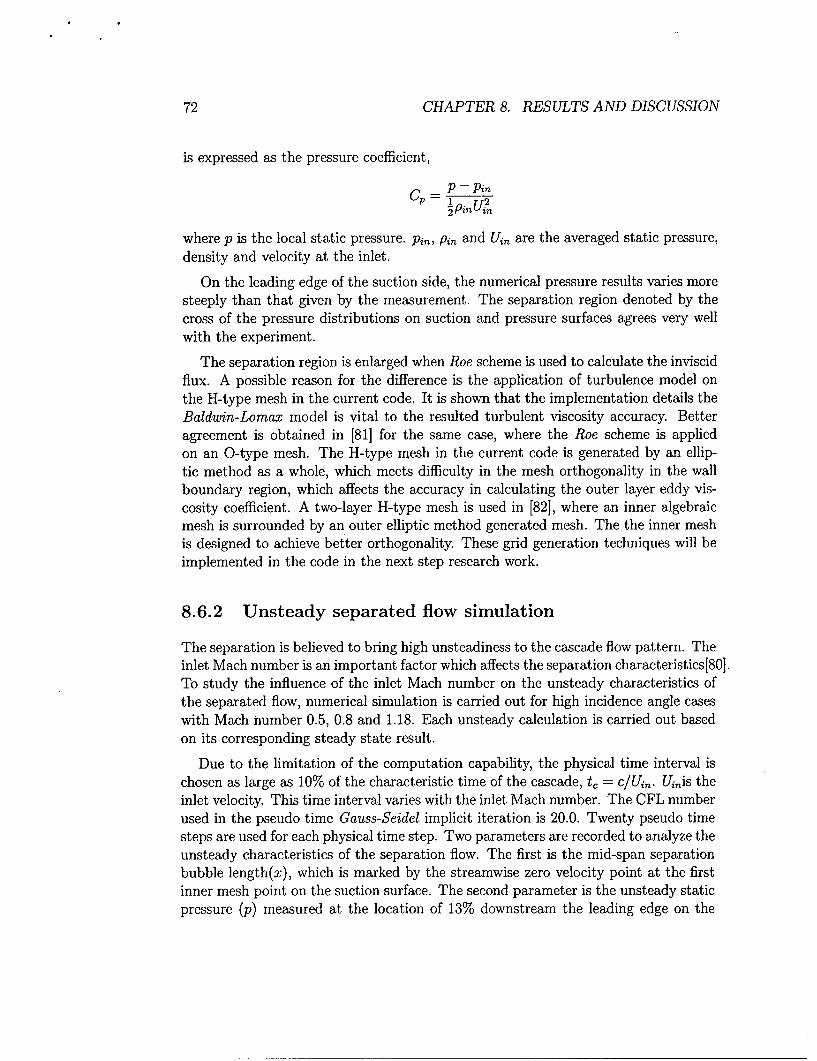
72 CHAPTER 8. RESULTS AND DISCUSSION
is expressed as the pressure coefficient,
P - Pin• Pin gn
where p is the local static pressure. Pin, Pin and Uin are the averaged static pressure,density and velocity at the inlet.
On the leading edge of the suction side, the numerical pressure results varies moresteeply than that given by the measurement. The separation region denoted by thecross of the pressure distributions on suction and pressure surfaces agrees very wellwith the experiment.
The separation region is enlarged when Roe scheme is used to calculate the inviscidflux. A possible reason for the difference is the application of turbulence model onthe H-type mesh in the current code. It is shown that the implementation details theBaldwin-Lomax model is vital to the resulted turbulent viscosity accuracy. Betteragreement is obtained in [81] for the same case, where the Roe scheme is appliedon an O-type mesh. The H-type mesh in the current code is generated by an ellip-tic method as a whole, which meets difficulty in the mesh orthogonality in the wallboundary region, which affects the accuracy in calculating the outer layer eddy vis-cosity coefficient. A two-layer H-type mesh is used in [82], where an inner algebraicmesh is surrounded by an outer elliptic method generated mesh. The the inner meshis designed to achieve better orthogonality. These grid generation techniques will beimplemented in the code in the next step research work.
8.6.2 Unsteady separated flow simulation
The separation is believed to bring high unsteadiness to the cascade flow pattern. Theinlet Mach number is an important factor which affects the separation characteristics [80].To study the influence of the inlet Mach number on the unsteady characteristics ofthe separated flow, numerical simulation is carried out for high incidence angle caseswith Mach number 0.5, 0.8 and 1.18. Each unsteady calculation is carried out basedon its corresponding steady state result.
Due to the limitation of the computation capability, the physical time interval ischosen as large as 10% of the characteristic time of the cascade, t, = c/Uin. Uinis theinlet velocity. This time interval varies with the inlet Mach number. The CFL numberused in the pseudo time Gauss-Seidel implicit iteration is 20.0. Twenty pseudo timesteps are used for each physical time step. Two parameters are recorded to analyze the
unsteady characteristics of the separation flow. The first is the mid-span separationbubble length(x), which is marked by the streamwise zero velocity point at the firstinner mesh point on the suction surface. The second parameter is the unsteady staticpressure (p) measured at the location of 13% downstream the leading edge on the
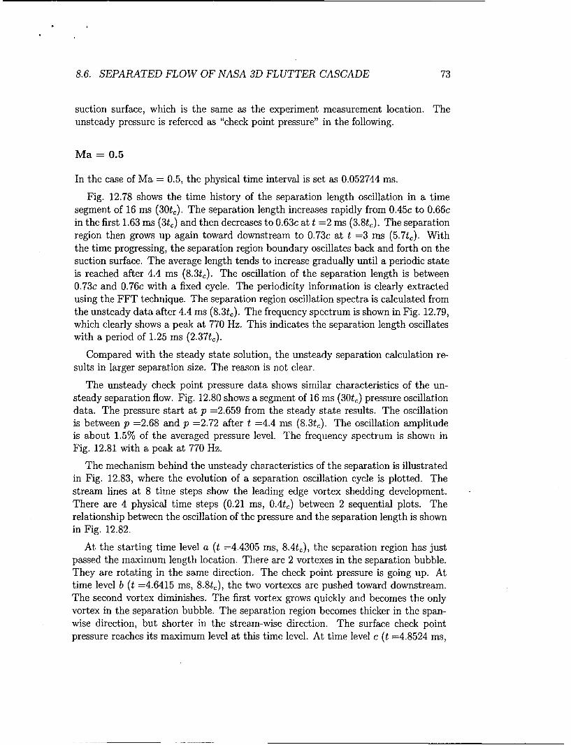
8.6. SEPARATED FLOW OF NASA 3D FLUTTER CASCADE 73
suction surface, which is the same as the experiment measurement location. Theunsteady pressure is refereed as "check point pressure" in the following.
Ma = 0.5
In the case of Ma = 0.5, the physical time interval is set as 0.052744 ms.
Fig. 12.78 shows the time history of the separation length oscillation in a timesegment of 16 ms (30t,). The separation length increases rapidly from 0.45c to 0.66cin the first 1.63 ms (3tQ) and then decreases to 0.63c at t =2 ms (3.8t,). The separationregion then grows up again toward downstream to 0.73c at t =3 ms (5.7t,). Withthe time progressing, the separation region boundary oscillates back and forth on thesuction surface. The average length tends to increase gradually until a periodic stateis reached after 4.4 ms (8.3t,). The oscillation of the separation length is between0.73c and 0.76c with a fixed cycle. The periodicity information is clearly extractedusing the FFT technique. The separation region oscillation spectra is calculated fromthe unsteady data after 4.4 ms (8.3t,). The frequency spectrum is shown in Fig. 12.79,which clearly shows a peak at 770 Hz. This indicates the separation length oscillateswith a period of 1.25 ms (2.37Q).
Compared with the steady state solution, the unsteady separation calculation re-sults in larger separation size. The reason is not clear.
The unsteady check point pressure data shows similar characteristics of the un-steady separation flow. Fig. 12.80 shows a segment of 16 ms (30Q) pressure oscillationdata. The pressure start at p =2.659 from the steady state results. The oscillationis between p =2.68 and p =2.72 after t =4.4 ms (8.3t,). The oscillation amplitudeis about 1.5% of the averaged pressure level. The frequency spectrum is shown inFig. 12.81 with a peak at 770 Hz.
The mechanism behind the unsteady characteristics of the separation is illustratedin Fig. 12.83, where the evolution of a separation oscillation cycle is plotted. Thestream lines at 8 time steps show the leading edge vortex shedding development.There are 4 physical time steps (0.21 ms, 0.4t,) between 2 sequential plots. Therelationship between the oscillation of the pressure and the separation length is shownin Fig. 12.82.
At the starting time level a (t =4.4305 ms, 8.4t,), the separation region has justpassed the maximum length location. There are 2 vortexes in the separation bubble.They are rotating in the same direction. The check point pressure is going up. Attime level b (t =4.6415 ms, 8.8t,), the two vortexes are pushed toward downstream.The second vortex diminishes. The first vortex grows quickly and becomes the onlyvortex in the separation bubble. The separation region becomes thicker in the span-wise direction, but shorter in the stream-wise direction. The surface check pointpressure reaches its maximum level at this time level. At time level c (t =4.8524 ms,

74 CHAPTER 8. RESULTS AND DISCUSSION
9.2t,), the separation bubble approaches its shortest length in stream-wise direction,and maximum thickness in the span-wise direction. The check point pressure isgoing down. At time level d (t = 5.0634ms, 9.6t,), the separation bubble has passedthe minimum length location, and begins to extend toward downstream. The checkpoint pressure is still going down. At time level e (t =5.2744 ms, 10.0t,), a newvortex is generated at leading edge and becomes the first vortex. The check pointpressure reaches its minimum value. The separation length is still increasing. At timelevel f (t=4854 ms, 10.4t,), the first vortex continues to grow. The second vortexis pushed toward downstream. Both the check point pressure and the separationlength are going up. The latter is approaching its maximum location. At time level g(t =5.6964 ms, 10.8t,), the two vortexes have almost the same size, the flow structureis close to the starting time level a. The separation boundary has passed its maximumlocation and begin to shrink toward upstream. The check point pressure is going up.At time level h (t =5.9073 ms, 11.2t,), the second vortex diminishes. A new cycle isstarted at this time level.
The leading edge vortex shedding exhibits obvious periodical pattern in its evolu-tion process. The leading edge keeps generating new vortexes. The new vortex pushesthe old vortex bubble toward downstream and the old vortex decreases in size at thesame time. When the two vortexes become of the same size, the maximum separa-tion length is reached, where the separation bubble has the thinnest size in span-wisedirection. As the new vortex grows further, the old vortex will diminish. The sepa-ration bubble will move upstream and makes the bubble thicker. The leading edgesurface check point pressure reaches its maximum level when the separation bubbleshrinks and reaches its minimum level when the separation bubble boundary extends.The vortex generation, pressure variation and separation length oscillation have thesame frequency characteristics with a phase difference as shown in Fig. 12.82. Suchoscillation is maybe one of the reasons to cause to flutter.
Ma = 0.8
The physical time interval used in the calculation for the case of Mach number 0.8 is0.0342 ms. A similar flowfield unsteady characteristics is exhibited in the computationresults.
Fig. 12.84 and Fig. 12.86 show the separation length and the checkpoint staticpressure oscillation history in a time period of 21 ms. A clear periodicity is shownin these two figures. It is found in the time averaged steady state study in [80] that,the increase of the inlet Mach number will enlarge the separation bubble in size.Fig. 12.86 indicates that the inlet Mach number increase also increases the amplitudeof the pressure oscillation. The oscillation amplitude is increased to about 5% ofthe averaged pressure level. The increased kinetic energy in the inflow bring higherunsteadiness intensity to the separated flow filed.

8.7. FORCED VIBRATION OF THE NASA FLUTTER CASCADE 75
The corresponding FFT frequency analysis is shown in Fig. 12.85 and Fig. 12.87respectively. The frequency analysis is based on the oscillation data after t=5 ms.The unsteady separation flow exhibits higher oscillation frequency because of theincreased inlet Mach number. A clear frequency spectrum peak is shown at 1400 Hzin both figures, twice the frequency in the case of Ma = 0.5.
Ma = 1.18
In the steady state simulation of the cascade at Ma=1.18 in [80], the separationflow characteristics are very different from those at subsonic. The further increasedkinetic energy in the inflow makes the flow attached to the blade surface in theleading edge. A smaller sized separation region appears after the shock wave becauseof the interaction of the shock wave and the turbulent boundary layer. The separationbubble shrinks in size and is located only in a small region at the center of the suctionsurface region.
The physical time interval in the calculation is set as 0.02483 ms. The pressurecheck point is located outside of the separation region in the supersonic case. Thepressure oscillation history is shown in Fig. 12.88. The oscillation amplitude is verysmall compared to the cases of Ma = 0.5 and Ma = 0.8. The flow tends to steady atthe leading edge. The pressure oscillation frequency spectrum is shown in Fig. 12.89.
The computed characteristics of the separation flow above is similar to the experi-ment measurement in [83]. In [83], when the blade is fixed, the blade surface pressurefor low subsonic inlet flow at Ma=0.5 and low supersonic inlet flow at Ma=1.1 ex-hibits very low unsteadiness and very strong self-induced oscillations with a frequencyof 110Hz is observed in high subsonic inlet flow at Ma=0.8. However, the strong lowfrequency oscillation is attributed to the tunnel resonance characteristics instead ofthe flow unsteadiness due to the flow separation in [84]. Even though, the cascadeflow separation is believed to have a direct relation with the wall surface pressureunsteady oscillation, which is an important factor to the flutter. Further detailednumerical research is necessary to discover the mechanism.
8.7 Forced Vibration of the NASA Flutter Cas-cade
8.7.1 Parameters used in flow analysis
The steady state static pressure coefficient is defined as the following,
C, (x/c) = p (1/c) - (8.16)U--2 -
76 CHAPTER 8. RESULTS AND DISCUSSION
where P0o, Po and U.. are the averaged pressure, density and velocity at inlet.
The blades vibrate harmonically with a constant IBPA. The motion of the nthblade is defined by the blade deflection angle[?],
a, (t) = ao + &Re [exp (i (wt + n/3))] (8.17)
where n is the blade index, t is the time, a0 is the deflection angle at the mean bladeposition, & is the amplitude of blade deflection, Re denotes the real part of a complexvalue, w is the angular frequency, 83 is the inter blade phase angle.
The reduced frequency k, is defined based on the chord length C as the following,
k,: = W (8.18)
The first harmonic unsteady pressure coefficient is defined as,
C'W Pi W (8.19)
where P, (x) is first harmonic pressure along the blade surface. It is a complex valueobtained from the unsteady pressure signals using the Fourier transformation. p (x)has a phase angle relative to the blade motion a.
The time dependent aerodynamic moment coefficient is defined as,
-J rp(x) ds
C(t) 1 U2 r (8.20)
where p (x) is the unsteady pressure along the blade surface, s is the surface area vectorpointing outward from the blade, r is the vector pointing from the pivot location toan arbitrary point x on the surface.
The imaginary part, or the out of phase part of the unsteady pressure determinesthe damping or excitation of the blade motion. The aerodynamic damping coefficientis defined as,
-E = -I m (Cm) (8.21)
where Im denotes the imaginary part of a complex value. A positive _ correspondsto a damped oscillation.
8.7.2 The Cascade
The NASA Lewis Oscillating Cascade test section consists of 9 identical airfoils withthe cross section similar to the tip airfoil of modern low-aspect ratio fan blades[?].

8.7. FORCED VIBRATION OF THE NASA FLUTTER CASCADE 77
The airfoil has a chord of 8.89 cm and is installed with a stagger angle of 600. Thesolidity is 1.52. In the experiment, the inlet Mach number is 0.5. All blades vibratesimultaneously along a pitching axis at 0.5 chord with a constant IBPA of 180'. Theoscillating amplitude is 1.2' and the reduced frequency based on chord varies at 0.4,0.8 and 1.2. The blade motion is identical on every other blade. The two neighboringblades always vibrate in opposite direction.
The inlet Mach number Ma = 0.5 is achieved by adjusting the outlet static pressurelevel. The Reynolds number based on the chord length is 9x 10'. The flow incidence is00. For the unsteady dual-time stepping, one physical blade oscillation cycle is dividedinto 100 time intervals and 100 pseudo time Gauss-Seidel iterations are carried out foreach physical time step. The 100 pseudo time iterations are proved to be sufficient toobtain a converged solution within a physical time step with the residual reduced by 3orders in magnitude. Before the unsteady simulation, the corresponding steady statecalculation is carried out to obtain the initial flow field for the unsteady computation.The inlet flow angle is adjusted to 610 to obtain good agreement with the steady stateexperimental surface pressure distribution.
Before the full scale computation; a simplified 2-passage cascade is computed witha reduced frequency of k, = 0.8 by applying the periodic boundary condition. Theinformation of the moving mesh and the conservative variables are exchanged acrossthe periodic boundary. The multi-passage full scale simulation is then conductedfor the 9-blade cascade with the wind tunnel side walls for more realistic results.The periodic boundary condition is not needed. The vibration frequencies of k,=0.4,0.8 and 1.2 are calculated and compared with the experiment measurement. Theinfluence of the end walls are studied by comparing the results of k,=0.8 from bothsimulations.
8.7.3 Computation domain decomposition and mesh gener-ation
As shown in Fig. 12.107, the computation domain which is consistent with the exper-iment configuration is split into 10 subdomains based on flow passages P1 throughP10. The 10 subdomains are computed by 10 CPUs running in parallel. The subdo-mains are separated from their neighbors by the blade surfaces BI through B9 and theMPI interface boundaries. The MPI interface boundaries are straight lines passingthrough the leading edge (LE) and trailing edge (TE) of the blades with appropriateangles in accord with the local flow direction. The pitchwise distance between theend wall and the blade is half of the inner pitch distance. The US (upper surface) isthe suction surface and LS (lower surface) is the pressure surface.
The inlet and outlet boundaries are set as 1.5 and 3 times chord length away fromthe airfoil LE and TE in axial direction. A part of the mesh is shown in Fig. 12.108

78 CHAPTER 8. RESULTS AND DISCUSSION
with the regions of LE and TE zoomed in for more details. The H-type mesh isgenerated for each subdomain respectively. Each subdomain shares the grid pointdistribution on the common MPI interface boundaries with its neighbors. To achievegood orthogonality on the blade surface, an additional algebraic boundary layer meshis generated in the wall surface region. As shown in Fig. 12.108, the grid lines areorthogonal on all blade surfaces except the small regions at LE and TE. The meshsize is 195(e) x 180(q) for all subdomains. For clarity, the mesh is plotted every 4 linesin the un-zoomed plots. The blade surface has 100 points in streamwise direction.The boundary layer has 40 points in pitchwise direction. Because of the high gradientof the flow variables in near wall region, the mesh is clustered near the wall surfaces.On the blade surfaces, the grid points are also clustered toward the LE and the TEin streamwise direction.
8.7.4 Simulation in two passage cascade
The two passage cascade simulation uses the meshes of two inner neighboring passages(P2 and P3) in the compressor cascade. As shown in Fig. 12.109, The blade betweenthe two passages is called BC (blade at center) and the two blade surfaces on the twooutside periodic boundaries are treated as blade BP (blade at periodic boundary) .
The steady state pressure coefficient distributions along the blade surfaces areplotted in Fig. 12.110. The pressure coefficient predicted agrees well with the mea-surement. The result on BC agrees very well with that of BP, which shows goodperiodicity is achieved on the pitchwise direction.
Fig. 12.111 shows the pressure variation history on two points on the suctionsurface (US) and the pressure surface (LS) respectively. The pressure on the suctionsurface is located at x/C = 0.15 and the pressure on the pressure surface is locatedat x/C = 0.1. The temporal periodicity is achieved very soon after the start of thevibration simulation. Because of the excellent temporal periodicity, the unsteadydata extracted from a single blade motion cycle is enough for the unsteady Fourieranalysis. The IBPA of 1800 is clearly shown by comparing the pressure maximumsand minimums on BC and BP.
The unsteady pressure coefficients are plotted in Fig. 12.112 and Fig. 12.113 forsuction surface (US) and the pressure surface (LS) respectively. The unsteady pres-sure coefficient Cp is expressed in terms of the real part or in phase part and theimaginary part or out of phase part. On the suction surface, as shown in Fig. 12.112,the CFD results compare fairly well with experiment data after 30% chord. The realpart of the coefficient is predicted lower than experiment data on leading edge, butthe trend agrees very well with the experiment. The imaginary part is over predictedin the leading edge region. On the pressure surface, as shown in Fig. 12.113, thereal part of the unsteady pressure coefficient agrees well with the experiment data.The imaginary part is under predicted compared with the measurement on the front

8.7. FORCED VIBRATION OF THE NASA FLUTTER CASCADE 79
part of the blade. This means that the CFD does not accurately capture the phaseangle difference between the pressure response and the blade motion. A local flutterstability analysis based on the aerodynamic work per cycle suggested by Buffum[?]is presented in Fig. 12.114 by plotting (0.5 - Im (Cp,upper - Cp,iower)lst. The cur-rent numerical simulation predicts a larger local stable region on the front part ofthe blade. On the aft part, the experiment data indicates a shallow stable region.The CFD predicts the trend very well. The aft part stable region is predicted moreshallow than the experiment.
8.7.5 Simulation in full scale cascade
The full scale steady and unsteady simulation use the same inlet flow angle as thatof the 2-passage case. In the steady state calculation, all blade are parallel to eachother at their mean positions. As shown in Fig. 12.107, the end wall is made up of 3sections, which have different angles relative to the x axis: a, = 61', a 2 = 600 anda 3 = 640. The middle section is parallel to the blade at its mean position. The frontand aft sections follow the inlet and outlet averaged flow directions obtained in the2-passage steady state computation.
The steady state Mach number contours for the full scale cascade is shown inFig. 12.115. The flow pattern is highly influenced by the end wall especially forthe near end wall passages, P1 and P10. The influence is reduced rapidly fromthe boundary passages to the inner passages. Good periodicity in flow pattern isachieved among the inner passages (P3 through P8). Three center blades, B4, B5and B6 are chosen to study the steady and unsteady periodicity in the rest of thepaper. Even though the periodicity looks good in the Mach contour plot, the staticpressure distribution still shows the influence of the end walls on different blades.
Fig. 12.116 shows the pressure coefficient chordwise distribution on the 3 centerblades. The experiment measurement and the 2-passage calculation results are alsoplotted for comparison. The surface pressure increases gradually from B4 to B6 onboth the pressure surface and the suction surface. The pressure distribution on bladeB6 is closest to the 2-passage periodic results on most part of the surfaces. Theexperiment measurement also shows the pressure variation on different blades[?], butits variation trend is opposite to the current numerical results. A possible reason forthis difference is that the inlet and outlet end wall angles used in the experiment maydiffer from the values used in the current simulation. The experimental angles are notavailable. Such a pitchwise flow pattern difference is also expected in the followingunsteady calculations.
The full scale unsteady simulation is first carried out for a reduced frequency k,0.8 to study the end wall influence on the periodicity of the blade unsteady char-
acteristics. Figs. 12.117 and 12.118 are the unsteady pressure coefficient chordwisedistribution on the 3 center blades compared with the 2-passage cascade and the ex-

80 CHAPTER 8. RESULTS AND DISCUSSION
periment results. On the upper surface, as shown in Fig. 12.117, the 3 blades havevery similar unsteady coefficients on most of the chordwise distance. The results ofblade B6 are closest to those of the 2-passage calculation. The difference between thefull scale results and the 2-passage results mainly locate at the front and center partof the blade. The full scale results agree with the experiment better in the centerpart. On the lower surface, as shown in Fig. 12.118, the full scale results of the 3blades are similar. The 2-passage results axe closer to the experiment data in the realpart.
As shown in Fig. 12.119, the full scale calculations predict higher stability on thefront part of the blade compared with the 2-passage results. The full scale results arecloser to the experiment measurement on the aft part of the blade. In the chordwiseregion of x/C = 0.5 to x/C=0.7, the measured stability is better predicted in the fullscale results. The 2-passage results shows instability in the same region. The end wallinfluence on the flow pattern periodicity is clearly shown in the unsteady aerodynamicmoment oscillation plots within a whole blade motion cycle in Fig. 12.120. Themoment is plotted versus the normalized deflection angle, a' = (a - a0 ) /&. Becauseof the end wall influence, the moment oscillations on the 3 center blades are different.They are also different from the 2-passage calculation results. The anti-clockwisedirection of all the unsteady moment curves indicates negative work acted by the fluidon the blade. The blade motion is therefore damped down by the fluid flow. Theblade motion is stable, which corresponds to a positive damping coefficient E. Thearea enclosed by the moment curve indicates the magnitude of the work exchangedbetween the fluid and the blade, which is also proportional to the magnitude of thedamping coefficient.
The damping coefficients on all the 9 blades in the full scale calculation versusthe blade number are shown in Fig. 12.121. The damping coefficient varies amongthe blades. The damping coefficients for blade B4, B5 and B6 are 0.67, 0.65 and0.68 respectively. Blade B1 has the lowest stability (=- =0.45) and blade B9 has thehighest stability (P = 1.4). The damping coefficient distribution is more uniform onthe center blades (B3 through B7), even though small variation exists. The bladestability in the full scale cascade depends on the location of the blade. The dampingcoefficient obtained in the 2-passage periodic computation is 0.55.
Fig. 12.122 plots a series of Mach number contours around blade B5 and B6. Aseparation bubble is generated and grows periodically on the leading edge of the suc-tion surface. At t =0, the two blades are initially located at their mean positionsand are parallel to each other. Blade B5 then rotates in the counter-clockwise di-rection with a negative deflection angle (nose down). At the same time, blade B6is rotating in the clockwise direction with a positive deflection angle (nose up). Att=0.2T, blade B5 is close to its minimum deflection position. The separation bubbleat its LE is pushed downstream and shrinks in size. At t=0.4T, blade B5 is rotatingback from its minimum deflection location toward its mean position, the separation

8.7. FORCED VIBRATION OF THE NASA FLUTTER CASCADE 81
bubble disappears from the suction surface. At t = 0.8T, a new separation bubbleis generated when blade B5 passes its maximum deflection position and rotates backtoward its mean position. The bubble obtains its maximum size when the blade isclose to its mean position. Similar phenomenon is observed on the neighboring bladeB6, but with a phase difference of 1800.
More extensive unsteady simulations are carried out for reduced frequencies k,0.4 and k, = 1.2. Figs. 12.123 and 12.124 show the unsteady pressure coefficientchordwise distribution of k, = 1.2. Similar to the results of k, = 0.8, the predictedunsteady complex pressure coefficients are close to each other on the 3 center blades,even though some small difference exists. As shown in Fig. 12.123, on the uppersurface, the imaginary parts of CFD results agree very well with the experimentresults except that it is over-predicted in the region of x/C=0.15 to x/C=0.40. Thereal part is also predicted quite well on the middle and aft part of the blade. Onthe lower surface, as shown in Fig. 12.124, the predicted real parts compare very wellwith experiment. The Imaginary part is under-predicted from LE to x/C = 0.7.
The local stability analysis for k, = 1.2 is plotted in Fig. 12.125. The correcttrend is predicted compared with the experiment measurement, even though themagnitude does not agree very well. The stability is over-predicted in LE region.The unstable region predicted on the front part of the blade is smaller than theexperiment results. The stability is predicted on the aft part, but the magnitude issmaller than the experiment data. The damping coefficients for all the blades areplotted in Fig. 12.126. The damping coefficients for blade B4, B5 and B6 are 0.81,0.78 and 0.84 respectively. The stability increases with the frequency. Similar to theresults of k, = 0.8, the most stable blade is blade B9 (-==1.5) and the least stableblade is blade BI (E=0.6). The damping coefficient is more uniformly distributedon the central blades. The variation of the damping coefficient on the center bladesincreases with the increasing frequency.
Because of the lack of experiment data, the unsteady pressure coefficient of k,=0.4is not presented for comparison. However, the local stability is analyzed and com-pared with the experiment data in Fig. 12.127. Similar to the results of k, = 0.8 andk, = 1.2, the trend is predicted well, but the magnitude differs from the experiment.As expected, the damping coefficient distribution is more uniform on center blades(Fig. 12.128). The variation of their magnitudes decreases with the decreasing vibra-tion frequency compared with the high frequency cases of k, = 0.8 and kc, 1.2. Thedamping coefficients on blade B4, B5 and B6 are 0.448, 0.446 and 0.434 respectively.The most stable blade is B9 with E = 1.02 and the least stable blade is B1 with =
0.28.
The unsteady aerodynamic moment oscillations on blade B5 under the 3 frequen-cies under investigation are plotted together and compared in Fig. 12.129. The damp-ing coefficient increase with the increasing frequency is indicated by the increasedarea enclosed by the unsteady moment oscillation curve. The local stability analysis

82 CHAPTER 8. RESULTS AND DISCUSSION
is summarized for all the 3 frequencies in Fig. 12.130. The computation results in-dicate higher stability near the leading edge for higher frequency vibration, which isconsistent with the experiment measurement. Even though the destabilization regionon the front part of the blade and the stability magnitude on the aft part of the bladepredicted by the numerical computation are smaller than those in the experiment,the trend is predicted well. Both the destabilization and stabilization increase withthe increasing frequency.
8.8 3D AGARD Wing Flutter Prediction
The result of steady state transonic ONERA M6 wing is calculated first in orderto validate CFD solver. Then, the flutter boundary of an AGARD wing 445.6 iscalculated.
8.8.1 Steady State Transonic ONERA M6 wing
As a validation of the three dimensional solver for a transonic wing, the steady statesolution of the transonic ONERA M6 wing is calculated. The freestream conditionsfor this study are listed in Table 8.8 below.
Table 8.8: Free-stream condition for ONERA M6 wing
Mach number 0.8395
Static Pressure (psia) 12.2913Temperature (R) 447.0
Angle-of-Attack (deg) 0.0Reynolds Number I 19.7x 10⁶
This case is calculated using an 0-type grid with the dimension of 144 (aroundwing) x60 (normal to the wing) x40 (spanwise). The far field boundary is located15 chords away from the chord center of the wing. The surface mesh of the wing isdepicted in Figure 12.133.
The Zha E-CUSP2 scheme is used to evaluate the inviscid fluxes with the 3rdorder MUSCL type differencing [85]. The turbulent Reynolds stress and heat flux arecalculated by the Baldwin-Lomax algebraic model[48J.
The computed surface pressure distributions at various cross sections are shown inFigure 12.134, together with the experimental data given by Schmitt et al. [86]. Thelocation of z/b = 0.2 is near the root, and z/b = 0.99 is at wing tip.
8.8. 3D AGARD WING FLUTTER PREDICTION 83
Overall, very good agreement is obtained between the computation and experimentfor each cross-section.
8.8.2 Validation of Structural Solver
To validate the structural model used in the present study, the dynamic responsesof a flexible plate wing shown in Figure 12.135 is calculated and compared with theresults by using the finite element solver ANSYS. The purpose of the study is to findout how many mode shapes are required for accurate representation of the structuralmotion under dynamic force.
The plate wing has the same outline as the AGARD wing 445.6, and its firstmode natural vibration frequency is nearly the same as the corresponding one of theAGARD wing 445.6. The thickness of the plate is 0.3", the root chord is 21.96", thetip chord is 14.49", and the spanwise length is 30". The plate wing consists of 80elements and 861 node points on each side of the wing. The plate wing is held fixedon the root.
A time-dependent force is exerted at node point 510 which is located at the mid-point of the wing tip. The three components of the force in the unit of pound are:
f, = 0.5sin(27rfet), fu = 0.3sin(27rfet), f2 = 0.8sin(2irfet) (8.22)
where the exciting frequency fe is equal to 10 Hz. The modal damping ratio (j = 0.01,the time step used is 0.0005 second. The dynamic responses at several locations arerecorded. Figure 12.136 shows the time histories of the responses at the node point491 which is located almost at the center of the plate wing. The numerical predictionsby the present structural solver with first five mode shapes agree excellently with theresults using ANSYS with first five mode shapes and the full model. The three resultsare virtually duplicated to each other and are indistinguishable.
8.8.3 AGARD Wing 445.6 Flutter
The AGARD 445.6 wing is selected to demonstrate the capability of the present solverfor predicting the flutter boundary. This wing has a quarter-chord sweep angle of 45degree, an aspect ratio of 1.65, a taper ratio of 0.6576, and a NACA65AO04 airfoilsection in the streamwise direction. The weakened wing model (Model 3) listed in[55] is chosen for this study. The geometry of the wing and its first six mode shapesas well as the experimental flutter results are also provided in the same report [55].The wing structure is modeled by its first five natural vibration modes in the presentcomputation.

84 CHAPTER 8. RESULTS AND DISCUSSION
The simulations start with the stationary rigid body wing model. After the steadystate flow field around the wing is fully developed, the rigid body wing is switched tothe flexible wing model. As a small imposed perturbation, the first mode displacementof the structural motion is set into sinusoidal motion for one cycle with the maximumamplitude of 0.0005 - 0.001 and the first mode frequency of the wing. Then the wingis allowed to deflect in response to the dynamic force load. Within each physical timestep, the solution is usually converged within 50 iterations.
In Figures 12.137 through 12.139 the time histories of generalized displacementsof the AGARD wing 445.6 at M,, = 0.96 are plotted for three different V*. In thesefigures, from V* = 0.26 to V* = 0.315, the plots correspond to the damped, neutral,and diverging responses, respectively. When the value of V* is smaller than thecritical value on the flutter boundary, the amplitudes of all modes decrease in timecorresponding to the damped response as shown in Figure 12.137. Once the valueof V* coincides with or is close to the critical value, the neutral response appears asshown in Fig. 12.138. When the value of V* is above the neutral stability point,the amplitudes of first five modes grow very fast, a diverging response is reached asshown in Fig. 12.139.
For a given Mach number, several runs with different V* are needed to determinethe location of the flutter boundary using bisection method. When V* is varied,the free-stream Reynolds number is changed accordingly. Strictly speaking, the free-stream Reynolds number needs to be updated and the initial steady-state flow fieldwith actual Reynolds number should be re-generated for each run. In present sim-ulation, the initial flow field and the Reynolds number remain unchanged when V*is varied since the effect on final solution due to small variation in the free-streamReynolds number is negligible when a turbulence model is used.
The comparison of computed flutter boundary and experimental data for AGARDWing 445.6 is illustrated in Figure 12.140. Overall, the computed results are in goodagreement with the experimental data. The "sonic dip" near Mach = 1.0 measured inthe experiment is very well captured by the computation. The discrepancy betweencomputed results and experimental data may be due to the inadequacy of the turbu-lent modeling to capture the shock/wave boundary layer interaction or may be dueto the inaccurate measurement in the experiment as suspected by some researchers.

Chapter 9
Personnel
The personnel participating this research include the PI, Dr. Gecheng Zha; Co-PT,Dr. Mingta Yang; the research associate, Dr. Xiangying Chen; and a Ph.D. student,Mr. Zongjun Hu, who has partially participated in this research.
85

86 CHAPTER 9. PERSONNEL

Chapter 10
Conclusions
In this research, a new high efficiency low diffusion upwind scheme is developed and isapplied to moving grid systems. The fully coupled fluid-structural interaction with thenew upwind scheme is successfully developed and predicts the 3d AGARD wing flutterboundary very well. The SNM model at time domain is developed and validated. Theforced vibration of the NASA flutter cascade is simulated with reasonable agreementwith the experiment. A set of nonlinear non-reflective boundary conditions for Navier-Stokes equations on the generalized coordinates is developed to avoid the reflectivewaves. The code is ready to calculate the fluid-structural interaction of the mistunnedrotor bladed disk. However, since the funding is only 3 years, which is one year shorterthan the 4 years time period originally proposed, the mistunned rotor simulation isnot completed and will be done in future when the funding is available.
The following is the specific conclusions achieved in this research:
10.1 The New E-CUSP scheme
A new efficient upwind scheme based on the concept of convective upwind and splitpressure (CUSP) is developed. The upwinding of the convective term and the pressuresplitting are consistent with their characteristics directions. The numerical dissipationof the new scheme at stagnation is low and is not greater than that of the Roe scheme.The scheme hence is able to resolve accurately wall boundary layers, and are able tocapture crisp shock waves and exact contact discontinuities. The performance of thenew scheme is compared with the Roe scheme, AUSM+ scheme, Van Leer scheme,and Van Leer-Hdnel scheme.
For the 1D Sod shock tube problem using Euler explicit scheme, the new schemehas the crispest shock profile and highest allowable CFL number of 1.0. For a slowlymoving contact surface, the new scheme is demonstrated to capture the exact contactsurface discontinuity with the maximum allowable CFL of 1.0, which is far greater
87

88 CHAPTER 10. CONCLUSIONS
than that of the other schemes. For a quasi-lD transonic nozzle, all the other schemesgenerate expansion shocks at the sonic point. The new scheme does not have theexpansion shock even though it has a glitch at the sonic point, which is due to thediscontinuity of the first derivative of the pressure splitting at sonic point.
For a Mach=2.0 supersonic adiabatic laminar flat plate boundary layer, the newscheme is able to accurately resolve the boundary layer velocity and temperatureprofiles using the first order differencing. The solution is as accurate as that of theRoe scheme and the AUSM+ scheme and hence demonstrates the low diffusion of thenew scheme.
For a transonic converging-diverging nozzle, oblique shock waves and reflectionsare crisply captured even though the shock waves do not align with the mesh lines.The predicted wall surface isentropic Mach number distribution agrees well with theexperiment. For a transonic inlet-diffuser with shock/turbulent boundary layer inter-action, the new scheme and the Roe scheme predict the surface pressure distributionsagreeing well with the experiment for the case of a weak shock. For the strong shockcase, both the new scheme and the Roe scheme over predict the strength of the shockwave. However, the pressure distribution predicted by the new scheme is closer tothe experiment. The AUSM+ solution has large pressure oscillations.
In the applications of the original Zha-Hu E-CUSP scheme, it is found that there istemperature oscillations near wall boundaries. The scheme is modified by replaceingthe pressure term with the total enthalpy in the smoothing factor of the energyequation. The temperature oscillations are removed in the modified scheme, which isnamed Zha E-CUSP2 scheme.
10.2 Non-Reflective Boundary Conditions
The non-reflective boundary conditions of Poinsot and Lele[33] for 3D Navier-Stokesequations are extended to the generalized coordinates in this paper. The character-istic form Navier-Stokes equations in conservative variables are given. The NRBC isapplied numerically in an implicit time marching method. The governing equationsfor inner domain and NRBC are solved simultaneously in a fully couple manner.
For the unsteady subsonic vortex propagating flow, the fixed pressure outflowboundary conditions imposing the exit pressure generates serious wave reflection andthe flow field is distorted, whereas, the NRBC developed in this paper generates cleanresults with no wave reflection and solution distortion.
For the transonic inlet-diffuser, the NRBC is not necessary for steady state solu-tions since the reflective waves are diffused when the solutions are converged. How-ever, for unsteady flows, the NRBC is essential. The fixed pressure outflow boundaryconditions generate strong reflective waves due to the shock/boundary layer inter-

10.3. 2D FLUTTER PREDICTION 89
action, which makes the shock oscillating motion far greater than the experimentaldata. When the NRBC is applied, the shock oscillation is dramatically reduced andthe computed time averaged pressure distributions and frequency spectrum agreemuch better with the experiment than FPBC.
The NRBC is essential for unsteady fluid-structural interactions, in particular forthe internal flows such as the mistunned rotors.
10.3 2D Flutter Prediction
The efficient high resolution E-CUSP upwind schemes developed in this researchhave been successfully extended and applied to calculate flow-induced vibration witha moving grid based on fully coupled fluid-structural interaction.
For an elastically mounted cylinder, various cases with different structural param-eters have been calculated. The predicted displacement agrees very well with theexperiment and the numerical results of other researchers.
For the forced pitching NACA 64A010 airfoil, the computed lift oscillation agreesaccurately with the experiment. The computed moment oscillation has large devia-tion from the experiment, but the results have a similar order of accuracy as otherresearchers have achieved. The discrepancy may be due to the inaccurate predictionof the surface shear stress caused by the inadequacy of the turbulence modeling andexperimental uncertainties.
The same airfoil has been calculated as an elastically mounted airfoil with freevibration in plunging and pitching directions. The computations have been carriedout using different values of velocity index V* which are below, close, and beyondthe critical point on the flutter boundary when Mach number is fixed. The corre-sponding responses of the airfoil flows are well simulated. The predicted value of V*at the bottom of the transonic dip is consistent with the numerical results of otherresearchers [5, 73, 70].
10.4 SNM model of Transient Response
The transient response (time domain) structural vibration model for mistunned rotorbladed disk based on the efficient Subsets of Nominal Modes (SNM) model is devel-oped. The vibration response results predicted by the SNM model for a full annulusbladed disk with blade frequency variation agree well with the results predicted by thefinite element model. The simplified model was designed such that transient responsecomputations can be performed in ANSYS with tractable computational cost. Thecomparison of the results showed that SNM model can capture both low frequency
90 CHAPTER 10. CONCLUSIONS
and high frequency responses. In the case of low frequency excitation, only one familyof blade modes is needed in SNM. In the case of high frequency excitation, multiplefamilies of blade modes are needed in SNM. The computational efficiency was im-proved by at least 30 times over ANSYS direct simulations for the cases examined.The improvement is expected to be much greater when high fidelity ANSYS modelsare needed.
10.5 Separated Flows in NASA 3D Flutter Cas-cade
1. The high incidence cascade separation flow shows a sinusoidal pattern on theoscillation of the surface pressure and the separation bubble size.
2. The leading edge vortex shedding is the mechanism behind the unsteady char-acteristics of the subsonic high incidence separation flow. New vortexes arecontinuously generated at the suction surface leading edge. The new vortexgrows and pushes the old vortexes downstream. The interaction between thevortexes results in the periodical oscillation of the separation bubble size andthe surface pressure. The vortex generation, pressure variation and separationlength oscillation have the same frequency characteristics with a phase differ-ence.
3. The characteristics of the separation flow is determined by the inlet Mach num-ber. When the inlet flow goes from lower subsonic to higher subsonic, thesize and the oscillation intensity of the separation bubble are enhanced. Theflowfield oscillation peak frequency increases. When the inflow goes further tosupersonic, the flow is attached on the leading edge. A small size separationbubble due to the interaction of the shock wave and the turbulent boundarylayer is located right after the shock wave.
10.6 Forced Vibration of the NASA Flutter Cas-cade
The fully nonlinear time dependent Navier-Stokes equations are solved with the paral-lel computation technique to simulate the unsteady flow field in a full scale compressorcascade with forced blade vibration. The calculation in this paper is conducted witha low incidence of 0' and a subsonic inflow M= 0.5. The blade motion amplitudeis 1.2'and the inter blade phase angle is 1800. The full scale computation is carriedout for 3 reduced frequencies, 0.4, 0.8 and 1.2. The blade stability under different

10.7. 3D AGARD WING FLUTTER PREDICTION 91
vibration frequency is analyzed. The end wall influence on the steady and unsteadyflow characteristics is studied by comparing the full scale results with the 2-passageperiodic cascade results at k, =0.8. The conclusions are the following:
1. The flow pattern in the full scale cascade shows that the flowfield is affected bythe existence of the end walls. The steady state blade surface pressure varieswith the the blade position in the cascade. The periodicity of the flow patternis improved by adjusting the end wall configuration. The end wall influenceattenuates rapidly from boundary passages to center passages. Good periodicityis achieved in the inner passages. The full scale computation gives better resultsof the unsteady pressure coefficient, local stability and aerodynamic momentamong the center blades.
2. All blades in the full scale cascade are stable, which is indicated by a positivedamping coefficient. The damping coefficient is more uniformly distributedon center blades. The most stable and the least stable blades are the twoboundary blades. The damping coefficient and its variation across the centerblades increase with the increasing vibration frequency.
3. The unsteady pressure coefficients are predicted well compared with the ex-periment measurement. The local stability trend is correctly predicted in thenumerical computation. The blade local stability is over-predicted on LE andunder-predicted on the aft part. The destabilization region located at the frontpart of the blade is predicted smaller compared with the experiment. The pre-dicted stabilization and destabilization increase with the increasing frequency,so do the damping coefficients.
10.7 3D AGARD Wing Flutter Prediction
A numerical methodology with fully coupled fluid-structural interaction for predi-cating 3-D transonic wing flutter has been developed. A dual-time step implicitunfactored Gauss-Seidel iteration with Roe scheme are employed in the flow solver.A modal approach structure solver is used to simulate the wing response. An effi-cient mesh deformation strategy based on an algebraic method is developed and isshown to be accurate and robust. The flow and structure solvers are fully coupled vissuccessive iterations within each physical time step.
The accuracy of the modal approach structure solver has been verified by usingthe finite element solver ANSYS. The results indicate that the first five modes aresufficient to accurately model the wing structure in the present study.
The computed flutter boundary of AGARD wing 445.6 for free stream Mach num-bers ranging from 0.499 to 1.141 is presented and compared well with the experimental

92 CHAPTER 10. CONCLUSIONS
data except for M, = 1.171, where the flutter boundary is over-predicted. The sonicdip is very well captured.
10.8 Future Work
With the foundation laid in the research, the next step is to apply the fully coupledfluid-structural interaction solver to mistunned rotor bladed disk.

Chapter 11
Publications
In this research project, we have published five journal publications, submitted twopapers for journal publications, and published 12 conference papers.
Journal Publications:
1) Chen, X. and Zha, G.-C., "Implicit Application of Non-Reflective Boundary Condi-tions for Navier-Stokes Equations in Generalized Coordinates ", International Journalfor Numerical Methods in Fluids, Vol. 50, No. 7, pp767-793, 2006
2) Chen, X. and Zha, G.-C.,"Fully Coupled Fluid-Structural Interactions Using anEfficient High Solution Upwind Scheme", Journal of Fluid and Structure, Vol. 20,No. 8, Nov. 2005, pp 1 105- 112 5
3) Zha, G.-C., "A Low Diffusion Efficient Upwind Scheme" , AIAA Journal, Vol.43,No.5, pp 1137-1140, 2005
4) Hu, Z. and Zha, G.-C.,"Calculations of 3D Compressible Using an Efficient LowDiffusion Upwind Scheme" ,International Journal for Numerical Methods in Fluids,Vol. 47, pp253-269, Nov. 2004
5) Zha, G.-C. and Hu, Z.," Calculation of Transonic Internal Flows Using an EfficientHigh Resolution Upwind Scheme" , AIAA Journal, Jan. 2004
Submitted for Journal Publication:
1) Chen, X., Zha, G.-C. and Yang, M.-T. "3D Simulation of a Transonic Wing Flut-ter using an Efficient High Resolution Upwind Scheme, to AIAA J. of Aircraft ",
Submitted for publication in AIAA Journal of Aircraft
2) Chen, X.-Y. and Zha, G.-C. and Yang, M.-T. "Numerical Simulation of 3-D WingFlutter with Fully Coupled Fluid-Structural Interaction " Submitted for publicationin Journal of Computer and Fluids
Conference Publications:
93
94 CHAPTER 11. PUBLICATIONS
1) Chen, X., Zha, G.-C. and Yang, M.-T. "3D Simulation of a Transonic Wing Flutterusing an Efficient High Resolution Upwind Scheme, to AIAA J. of Aircraft ", AIAAPaper 2006-3216, 36th AIAA Fluid Dynamics Conference and Exhibit, June 5-8, 2006,San Franscisco, CA
2) Hu, Z. and Zha, G.-C. "Parallel Computation of Forced Vibration for A CompressorCascade ", AIAA Paper 2006-0628, AIAA the 44th Aerospace Sciences Meeting andExhibit Conference, Jan. 8-12, 2006, Reno, NV
3) Chen, X.-Y. and Zha, G.-C. and Yang, M.-T. "Numerical Simulation of 3-D WingFlutter with Fully Coupled Fluid-Structural Interaction ", AIAA Paper 2006-0697,AIAA the 44th Aerospace Sciences Meeting and Exhibit Conference, Jan. 8-12, 2006,Reno, NV
4) Chen, X. and Zha, G.-C., "Implicit Application of Non-Reflective Boundary Con-ditions for Navier-Stokes Equations in Generalized Coordinates ", AIAA Paper 2005-0091, AIAA the 43rd Aerospace Sciences Meeting and Exhibit Conference, Jan. 10-13,2005, Reno, NV
5) Hu, Z. and Zha, G.-C.,"Simulation of 3D Flows of Propulsion Systems Usingan Efficient Low Diffusion E-CUSP Upwind Scheme",AIAA Paper 2004-4082, 40thAIAA/ASME/SAE/ASEE Joint Propulsion Conference and Exhibit, July 11-14, FortLauderdale, Florida
6) Chen, X. and Zha, G.-C.,"Fully Coupled Fluid-Structural Interactions Using anEfficient High Solution Upwind Scheme" , AIAA Paper 2004-2331, 34th AIAA FluidDynamics Conference and Exhibit, 28 Jun - 1 Jul 2004, Portland, Oregon
7) Chen, X. Zha, G.-C. and Hu, Z.,"Numerical Simulation of Flow Induced VibrationBased on Fully Coupled Fluid-Structural Interactions" , AIAA Paper 2004-2240, 34thAIAA Fluid Dynamics Conference and Exhibit, 28 Jun - 1 Jul 2004, Portland, Oregon
8) Zha, G.-C., "A Low Diffusion E-CUSP Upwind Scheme for Transonic Flows " ,AIAA Paper 2004-2707, 34th AIAA Fluid Dynamics Conference and Exhibit, 28 Jun- 1 Jul 2004, Portland, Oregon
9) Hu, Z. and Zha, G.-C.," Numerical Study of a Casacde Unsteady Separated Flow"ASME Paper GT2004-53195, ASME TURBO EXPO 2004, June 14-17, 2004, Vienna,Austria
10) Chen, X., Zha, G.-C., Hu, Z. and Yang, M.-T.,"Flutter Prediction Based on FullyCoupled Fluid-Structural Interactions" , paper, 9th National Turbine Engine HighCycle Fatigue Conference, 16-19 March 2004
11) Zha, G.-C. and Hu, Z., "Calculation of Transonic Internal Flows Using an Effi-cient High Resolution Upwind Scheme" , AIAA-2004-1097, AIAA the 42st AerospaceSciences Meeting and Exhibit Conference, Jan. 5-8, 2004, Reno, NV
12) Zha, G.-C. and Hu, Z.,"Numerical Study on Flow Separation of A Transonic
95
Cascade" , AIAA-2004-0199, AIAA the 42st Aerospace Sciences Meeting and ExhibitConference, Jan. 5-8, 2004, Reno, NV
96 CHAPTER 11. PUBLICATIONS

Chapter 12
Acknowledgment
The funding support from AFOSR for this research with grant F49620-03-1-0253 isacknowledged. The authors would like to thank the program manager Dr. FaribaFahroo at AFOSR for her support of this research. The authors would also like tothank the management of Pratt & Whitney to support this research collaborationwith the cost sharing.
97

98 CHAPTER 12. ACKNOWLEDGMENT

Bibliography
[1] G.-C. Zha and Z.-J. Hu, "Calculation of Transonic Internal Flows Using an Effi-cient High Resolution Upwind Scheme," AIAA Journal, vol. 42, No. 2, pp. 205-214, 2004.
[2] X. Chen and G.-C. Zha, "Fully Coupled Fluid-Structural Interactions Using anEfficient High Solution Upwind Scheme," Journal of Fluid and Structure, vol. 20,pp. 1105-1125, 2005.
[3] G.-C. Zha, "Low Diffusion Efficient Upwind Scheme ," AIAA Journal, vol. 43,2005.
[4] X.-Y. Chen, G.-C. Zha, and M.-T. Yang, "Numerical Simulation of 3-D WingFlutter with Fully Coupled Fluid-Structure Interaction Approach." AIAA Paper2006-0697, 44th AIAA Aerospace Sciences Meeting and Exhibit, Reno, NA,,Revised for publication in the Journal of Computer & Fluids, July 2006.
[5] X.-Y. Chen, G.-C. Zha, and Z.-J. Hu, "Numerical Simulation of Flow InducedVibration Based on Fully Coupled-Structural Interactions." AIAA Paper 2004-2240, AIAA 34th AIAA Fluid Dynamics Conference,, Jaun 28 - July 1, 2004.
[6] X. Chen and G.-C. Zha, "Implicit Application of Non-Reflective Boundary Con-ditions for Navier-Stokes Equations in Generalized Coordinates," InternationalJournal for Numerical Methods in Fluids, vol. 50, 2006.
[7] R. B. Melville, "Next Generation Computational Tools for Next Generation Chal-lenges." AFOSR/AFRL Workshop on Nonlinear Aspects of Aeroelasticity, March6-7, 2003.
[8] P. D. Silkowski, C. M. Rhie, G. S. Copeland, J. A. Eley, and J. M. Bleeg, " CFDInvestigation of Aeromechanics ." ASME Paper 2001-GT-0267, Proceedings ofASME TURBO EXPO 2001, New Orleans, Louisiana., June 4-7, 2001.
[9] G. Hilbert and A. Blair, "Accuracy of Airfoil Resonance Stress Predictions."Proceedings of the 6th National Turbine Engine High Cycle Fatigue (HCF) Con-ference, Jacksonville, Florida, 5-8 March 2001.
99

100 BIBLIOGRAPHY
[10] 0. Bendiksen and K. Kousen, "Transonic Flutter Analysis Using the Euler Equa-tions." AIAA Paper 87-0911, 1987.
[11] J. J. Alonso and A. Jameson, "Fully-Implicit Time-Marching Aeroelastic Solu-tions." AIAA Paper 94-0056, 1994.
[12] J. J. Alonso, L. Martineli, and A. Jameson, "Multifrid Unsteady Navier-StokesCalculations with Aeroelastic Applications." AIAA Paper 95-0048, 1995.
[13] F. Liu, J. Cai, Y. Zhu, A. Wong, and H. Tsai, "Calculation of Wing Flutter bya Coupled CFD-CSD Method." AIAA-2000-0907, 2000.
[14] R. B. Melville and S. A. Morton, "Fully Implicit Aeroelasticity on Oveerset GridSystems ." AIAA Paper-98-0521, 1998.
[15] A. Sayma, J. Vahdati, M. Green, and M. Imregun, "Whole-assembly FlutterAnalysis of a Low Pressure Turbine Blade," The Aeronautical Journal, vol. 102,pp. 459-463, 1998.
[16] A. Sayma, M. Vahdati, and M. Imregun, "Turbine Forced Response Predic-tion Using an Integrated Nonlinear Analysis ," Journal of Multi-body Dynamics,vol. 214(K1), pp. 45-60, 2000.
[17] A. Sayma, M. Vahdati, and M. Imregun, "Multi-stage whole-annulus forced re-sponse predictions using an integrated non-linear analysis technique - Part I:Numerical model," Journal of Fluids & Structures, vol. 14(1), pp. 87-101, 2000.
[18] A. Sayma, M. Vahdati, and M. Imregun, "Multi-stage whole-annulus forced re-sponse predictions using an integrated non-linear analysis technique - Part II:Study of a HP turbine," Journal of Fluids & Structures, vol. 14(1), pp. 103-125,2000.
[19] H. Doi and J. J. Alonso, "Fluid/Structure Coupled Aeroelastic Computationsfor Transonic Flwos in Turbomachinery." GT-2002-30313, June 3-6, 2002.
[20] A. Jameson, "Analysis and Design of Numerical Schemes for Gas DynamicsI: Artificial Diffusion, Upwind Biasing, Limiters and Their Effect on Accuracyand Multigrid Convergence in Transonic and Hypersonic Flow." AIAA Paper93-3359, July, 1993.
[21] A. Jameson, "Analysis and Design of Numerical Schemes for Gas Dynamics I:Artificial Diffusion, Upwind Biasing, Limiters and Their Effect on Accuracy andMultigrid Convergence in Transonic and Hypersonic Flow," Journal of Compu-tational Fluid Dynamics, vol. 4, pp. 171-218, 1995.
BIBLIOGRAPHY 101
[22] A. Jameson, "Analysis and Design of Numerical Schemes for Gas Dynamics II:Artificial Diffusion and Discrete Shock Structure," Journal of ComputationalFluid Dynamics, vol. 5, pp. 1-38, 1995.
[23] M.-S. Liou, "A Sequel to AUSM: AUSM+," Journal of Computational Physics,vol. 129, pp. 364-382, 1996.
[24] D. Hdnel, R. Schwane, and G. Seider, "On the Accuracy of Upwind Schemes forthe Solution of the Navier-Stokes Eqautions." AIAA paper 87-1105 CP, 1987.
[25] J. R. Edwards, "A Low-Diffusion Flux-Splitting Scheme for Navier-Stokes Cal-culations." AIAA Paper 95-1703-CP, June, 1995.
[26] J. R. Edwards, "A Low-Diffusion Flux-Splitting Scheme for Navier-Stokes Cal-culations," Computer & Fluids, vol. 6, pp. 635-659, 1997.
[27] X.-Y. Chen and G.-C. Zha, "Fully Coupled Fluid-Structural Interactions Usingan Efficient High Resolution Upwind Scheme," Journal of Fluids and Structures,vol. 20, pp. 1105-1125, 2005.
[28] X.-Y. Chen and G.-C. Zha, "Calculation of 3D Transonic Wing Flutter Using anEfficient High Resolution Upwind Scheme." AIAA-2006-3216, 36th AIAA FluidDynamics Conference and Exhibit, San Francisco, CA, 5-8 June, 2006.
[29] E. Lee-Rausch and J. Batina, "Calculation of AGARD Wing 445.6 Flutter UsingNavier-Stokes Aerodynamics." AIAA Paper 93-3476, 1993.
[30] S. A. Morton, R. B. Melville, and M. R. Visbal, "Accuracy and Coupling Issuesof Aeroelastic Navier-Stokes Solutions on Deforming Meshes." AIAA Paper-97-1085, 1997.
[31] R. B. Melville, S. A. Morton, and D. P. Rizzetta, "Implementation of a Fully-Implicit, Aeroelastic Navier-Stokes Solver." AIAA Paper-97-2039, 1997.
[32] R. Gordnier and M. R.B., "Transonic Flutter Simulations Using an ImplicitAeroelastic Solver," Journal of Aircraft, vol. 37, pp. 872-879, September-October2000.
[33] T. Poinsot and S. Lele, " Boundary Conditions for Direct Simulations of Com-pressible Viscous Flows," Journal of Computational Physics, vol. 101, pp. 104-129, 1992.
[34] T. Nishizawa and H. Takata, " Numerical Study on Rotating Stall in FinitePitch Cascades." ASME Paper., Proceedings of the International Gas Turbineand Aeroengine Congress and Exposition, The Hague, Netherlands, June 1994.
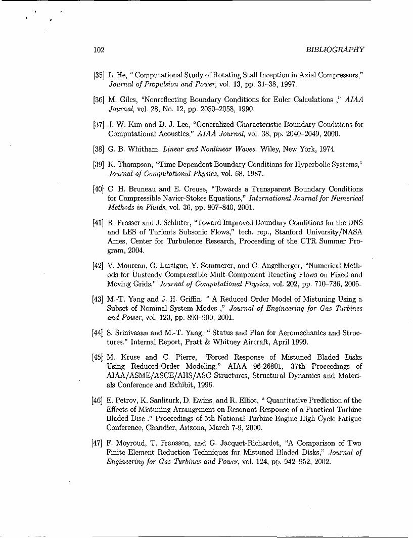
p
102 BIBLIOGRAPHY
[35] L. He, "Computational Study of Rotating Stall Inception in Axial Compressors,"Journal of Propulsion and Power, vol. 13, pp. 31-38, 1997.
[36] M. Giles, "Nonreflecting Boundary Conditions for Euler Calculations ," AIAAJournal, vol. 28, No. 12, pp. 2050-2058, 1990.
[37] J. W. Kim and D. J. Lee, "Generalized Characteristic Boundary Conditions forComputational Acoustics," AIAA Journal, vol. 38, pp. 2040-2049, 2000.
[38] G. B. Whitham, Linear and Nonlinear Waves. Wiley, New York, 1974.
[39] K. Thompson, "Time Dependent Boundary Conditions for Hyperbolic Systems,"Journal of Computational Physics, vol. 68, 1987.
[40] C. H. Bruneau and E. Creuse, "Towards a Transparent Boundary Conditionsfor Compressible Navier-Stokes Equations," International Journal for NumericalMethods in Fluids, vol. 36, pp. 807-840, 2001.
[41] R. Prosser and J. Schluter, "Toward Improved Boundary Conditions for the DNSand LES of Turlents Subsonic Flows," tech. rep., Stanford University/NASAAmes, Center for Turbulence Research, Proceeding of the CTR Summer Pro-gram, 2004.
[42] V. Moureau, G. Lartigue, Y. Sommerer, and C. Angelberger, "Numerical Meth-ods for Unsteady Compressible Mult-Component Reacting Flows on Fixed andMoving Grids," Journal of Computational Physics, vol. 202, pp. 710-736, 2005.
[43] M.-T. Yang and J. H. Griffin, " A Reduced Order Model of Mistuning Using aSubset of Nominal System Modes ," Journal of Engineering for Gas Turbinesand Power, vol. 123, pp. 893-900, 2001.
[44] S. Srinivasan and M.-T. Yang, "Status and Plan for Aeromechanics and Struc-tures." Internal Report, Pratt & Whitney Aircraft, April 1999.
[45] M. Kruse and C. Pierre, "Forced Response of Mistuned Bladed DisksUsing Reduced-Order Modeling." AIAA 96-26801, 37th Proceedings ofAIAA/ASME/ASCE/AHS/ASC Structures, Structural Dynamics and Materi-als Conference and Exhibit, 1996.
[46] E. Petrov, K. Sanliturk, D. Ewins, and R. Elliot, " Quantitative Prediction of theEffects of Mistuning Arrangement on Resonant Response of a Practical TurbineBladed Disc ." Proceedings of 5th National Turbine Engine High Cycle FatigueConference, Chandler, Arizona, March 7-9, 2000.
[47] F. Moyroud, T. Fransson, and G. Jacquet-Richardet, "A Comparison of TwoFinite Element Reduction Techniques for Mistuned Bladed Disks," Journal ofEngineering for Gas Turbines and Power, vol. 124, pp. 942-952, 2002.
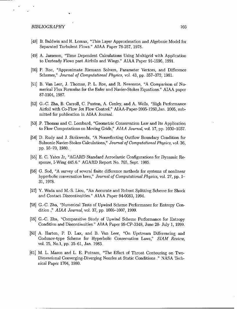
BIBLIOGRAPHY 103
[48] B. Baldwin and H. Lomax, "Thin Layer Approximation and Algebraic Model forSeparated Turbulent Flows." AIAA Paper 78-257, 1978.
[49] A. Jameson, "Time Dependent Calculations Using Multigrid with Applicationto Unsteady Flows past Airfoils and Wings." AIAA Paper 91-1596, 1991.
[50] P. Roe, "Approximate Riemann Solvers, Parameter Vectors, and DifferenceSchemes," Journal of Computational Physics, vol. 43, pp. 357-372, 1981.
[51] B. Van Leer, J. Thomas, P. L. Roe, and R. Newsome, "A Comparison of Nu-merical Flux Formulas for the Euler and Navier-Stokes Equations." AIAA paper87-1104, 1987.
[52] G.-C. Zha, B. Carroll, C. Paxton, A. Conley, and A. Wells, "High PerformanceAirfoil with Co-Flow Jet Flow Control." AIAA-Paper-2005-1260,Jan. 2005, sub-mitted for publication in AIAA Journal.
[53] P. Thomas and C. Lombard, "Geometric Conservation Law and Its Applicationto Flow Computations on Moving Grids," AIAA Journal, vol. 17, pp. 1030-1037.
[54] D. Rudy and J. Strikwerda, "A Nonreflecting Outflow Boundary Condition forSubsonic Navier-Stokes Calculations," Journal of Computational Physics, vol. 36,pp. 55-70, 1980.
[55] E. C. Yates Jr, "AGARD Standard Aeroelastic Configurations for Dynamic Re-sponse, I-Wing 445.6." AGARD Report No. 765, Sept. 1985.
[56] G. Sod, "A survey of several finite difference methods for systems of nonlinearhyperbolic conversation laws," Journal of Computational Physics, vol. 27, pp. 1-31, 1978.
[57] Y. Wada and M.-S. Liou, "An Accurate and Robust Splitting Scheme for Shockand Contact Discontinuities." AIAA Paper 94-0083, 1994.
[58] G.-C. Zha, "Numerical Tests of Upwind Scheme Performance for Entropy Con-dition ," AIAA Journal, vol. 37, pp. 1005-1007, 1999.
[59] G.-C. Zha, "Comparative Study of Upwind Scheme Performance for EntropyCondition and Discontinuities." AIAA Paper 99-CP-3348, June 28- July 1, 1999.
[60] A. Harten, P. D. Lax, and B. Van Leer, "On Upstream Differencing andGodunov-type Scheme for Hyperbolic Conservation Laws," SIAM Review,vol. 25, No.1, pp. 35-61, Jan. 1983.
[61] M. L. Mason and L. E. Putnam, "The Effect of Throat Contouring on Two-Dimensional Converging-Diverging Nozzles at Static Conditions ." NASA Tech-nical Paper 1704, 1980.

104 BIBLIOGRAPHY
[62] T. Bogar, M. Sajben, and J. Kroutil, "Characteristic Frequency and LengthScales in Transonic Diffuser Flow Oscillations." AIAA Paper 81-1291, 1981.
[63] A. Roshko, "On the Development of Turbulent Wakes From Vortex Streets."NACA Rep. 1191, 1954.
[64] S. Goldstein, "Modern Developments in Fluid Dynamics." Clarendon Press, Ox-ford, 1938.
[65] J. Alonso, L. Martinelli, and A. Jameson, "Multigrid Unsteady Navier-StokesCalculations with Aeroelastic Applications." AIAA Paper 95-0048, 1995.
[661 A. Roshko, "On the development of turbulent wakes from vortex streets," Tech.Rep. NACA Technical Note 2913, NACA, March 1953.
[67] 0. M. Griffin, "Vortex-induced vibrations of marine structures in uniform andsheared currents." NSF Workshopon Riser Dynamics, University of Michigan,1992.
[68] H. Blackburn and G. Karniadakis, "Two and Three-Dimensional Vortex-InducedVibration of a Circular Cylinder." ISOPE-93 Conference, Singapore, 1993.
[69] P. Cook, M. McDonald, and M. Firmin, "Aerofoil RAE 2822 - Pressure Distri-butions, and Boundary Layer and Wake Measurements." AGARD Report AR138, 1979.
[70] B. B. Prananta, H. M. H. L., and Z. R. J., "Two-Dimensional Transonic Aeroe-lastic Analysis Using Thin-Layer Navier-Stokes Method," Journal of Fluid and
Structures, vol. 12, pp. 655-676, 1998.
[71] S. S. Davis, "Naca 64 a010 (naca ames model) oscillatory pitching," Tech. Rep.AGARD Report No. 702, AGARD, August 1982.
[72] M. McMullen, A. Jameson, and J. Alonso, "Application of a Non-Linear Fre-quency Domain Solver to the Euler and Navier-Stokes Equations." AIAA Paper-2002-0120, 2002.
[73] J. Bohbot and D. Darracq, "Time Domain Analysis of Two D.O.F. Airfoil FlutterUsing an Euler/Turbulent Navier-Stokes Implicit Solver." International Forumon Aeroelasticity and Structural Dynamics, Madrid, Spain, June 5-7, 2001.
[74] K. Isogai, "Transonic Dip Mechanism of Flutter of a Sweptback Wing: Part II,"AIAA Journal, vol. 19, pp. 1240-1242, September 1981.
[75] J. J. Alonso and A. Jameson, "Fully-Implicit Time-Marching Aeroelastic Solu-tions." AIAA Paper 94-0056, 1994.

BIBLIOGRAPHY 105
[76] K. Kousen and 0. Bendiksen, "Nonlinear Aspects of the Transonic AeroelasticStability Problem." AIAA Paper 88-2306, 1988.
[77] T. Hsieh, T. J. Bogar, and T. J. Coakley, "Numerical Simulation and Comparisonwith Experiment for Self-Excited Oscillations in a Diffuser Flow," AIAA Journal,vol. 25, No. 7, July, 1987.
[78] J. Lepicovsky, E. McFarland, R. Chima, and J. Wood, "On Flowfield Peri-odicity in the NASA Transonic Flutter Cascade, Part I-Experimental Study."NASA/TM-2000-209934, ASME 2000-GT-0572, 2000.
[79] D. H. Buffum, V. R. Capece, A. J. King, and Y. M. EL-Aini, "Oscillating cascadeaerodynamics at large mean incidence." NASA Technical Memorandum 107247,1996.
[80] Z. Hu, G. Zha, and J. Lepicovsky, "Numerical study on flow separation of atransonic cascade," Jan. 2004. AIAA Paper 2004-0199.
[81] B. Griiber and V. Carstens, "The impact of viscous effects on the aerodynamicdamping of vibrating transonic compressor blades-a numerical study," Journalof Turbomachinery, vol. 123, 2001.
[82] S. Weber and M. F. Platzer, "A Navier-Stokes analysis of the stall flutter char-acteristics of the Buffum cascade," Journal of Turbomachinery, vol. 122, 2000.
[83] J. Lepicovsky, E. R. McFarland, V. R. Capece, and J. Hayden, "Unsteady pres-sures in a transonic fan cascade due to a single oscillating airfoil." ASME PaperGT-2002-30312, 2002.
[84] J. Lepicovsky, V. R. Capece, and C. T. Ford, "Resonance effects in the NASAtransonic flutter cascade facility." ASME Paper GT-2003-38344, 2003.
[85] B. Van Leer, "Towards the Ultimate Conservative Difference Scheme, III," Jour-nal of Computational Physics, vol. 23, pp. 263-75, 1977.
[86] V. Schmitt and F. Charpin, "Pressure Distributions on the ONERA-M6-Wingat Transonic Mach Numbers," Tech. Rep. AGARD AR 138, AGARD, May 1979.

106 BIBLIOGRAPHY
1.41.4
Zha E-CUSP, CFL=1.00 D
0 _____ Van Leer, CFLaO0.96 0Theory o o Theory 0
0 0
1.2 0
1.21z
o3
- 0
E ECL CL
0 10
0.8 130.8D
0.60 L .,, 5. i 11 n A n 0.60 1 . . . 51 L . .0 . .
XIL XIL
Figure 12.1: Temperature distribution of Figure 12.3: Temperature distribution ofthe Sod 1D shock tube computed by Zha the Sod 1D shock tube computed by VanE-CUSP scheme Leer scheme
1.40 4 1.4o S o Van Leer-Hanel CFLI.00
Roe Scheme, CFL=O.95 o To Theory T
1.2 o 1o
0 ,1.2 0
CL CLE Er CI-- I-.
0 10
0.8 00.8
5 10 0 5 10
X/L XIL
Figure 12.2: Temperature distribution of Figure 12.4: Temperature distribution ofthe Sod 1D shock tube computed by Roe the Sod 1D shock tube computed by Vanscheme Leer-Hinel scheme

BIBLIOGRAPHY 107
0.51.4
0.4 Roe Scheme00.4 -STheory o CFL=0.35
0 LUou AUSM+, CFL=0.275 0 0.3 7o 0.3
0
r, 0.1
0
'0 >0EDI - -0 .1
0 -0.2
-0.3
0.65 10 5 10X/L XlL
Figure 12.5: Temperature distribution Figure 12.7: Computed density profile ofof the Sod 1D shock tube computed by a slowly moving contact surface using theAUSM+ scheme Roe scheme
11 - 11 0.14
10 0 ZhaCUSP, CFL=1.00 10"- Van Leer, CFL=O.5S
9 0 Roe Scheme, CFL=0.3 9 ' Van Leer-Hanel
8 & AUSM, CFL=0.48 8 8 - CFL=.5
070 7 0.116 62
40.1S5, 5 00.o 0. 0 9ý
S4 .: 4
3 3 0.080
2 20.07
0.061 - 1
0•- 0 0.06
-1 . I . . . . -1 . _. _. _._._._._._._ _ _ _ 0.055 10 5 10
XIL XIL
Figure 12.6: Computed density and ve- Figure 12.8: Computed density and ve-locity profiles of a slowly moving contact locity profiles of a slowly moving contactsurface surface

108 BIBLIOGRAPHY
3
- - ZhaCUSP
2.5 Theoq 14
-- -- ,-- -Roo Schem.LlouAUSM" 12 Zha CUSP
2 VanLeer-Hanel 0 Blaslus
E -- - VanLeerFVS - Roe Scheme
Z 10 -.---.- Van Leer-Hanel
Van Leer FVSS1...- ..--- LiouAUSM+
0246880.5 4' "-
0 2 4 6 82
X/h
1,.2 1.4 1.6
Figure 12.9: Computed Mach numb Trr
distributions for the converging-divergingnozzle Figure 12.11: Computed temperature
profiles of the laminar boundary layer us-ing 1st order schemes
14 ____1 Zha CUSP
a Blasius
12 Roe Sch me-- - - - UouAUSM÷---.. --- Van Leer-Hanel
10 - .-------- Van Leer FVS
8Se
6 I
4 /
2
0 0.2 0.4 0.6 0.8 1
U/Ur
Figure 12.12: Computed Mach numberFigure 12.10: Computed velocity profiles contours using the Zha CUSP schemeof the laminar boundary layer using 1storder schemes

BIBLIOGRAPHY 109
0.9
0.8
1.5
1.4 1.4 0.7
1.3
i 1.2 0.E 1.1L 0.6
Z0 Experiment-- Zha CUSP Scheme
0.9 0.5 -. Roe Scheme•) O Experiment
0.8-.... Zha CUSP 175x50
Zha CUSP 175x80-0.-.-.- Roe Scheme 175x50 0.4
0.6 . . Roe Scheme 175x80
0.30.4 0 5A
,,_, _ _,_ _,,_,_.. ... .. , . .. ...... X IH-0.3 -0.2 -0.1 0 0.1 0.2 0.3 0.4 0.5 0.6 0.7 0.8 0.9 1
XlL
Figure 12.15: Static pressure distributionFigure 12.13: Adiabatic Mach number computed on the upper surface of thedistribution computed on the wall surface inlet-diffuser (Pout/Pt = .83)of the nozzle
0.9
0.8 0 Expedment
0.8___ Zha CUSP Scheme- -.. . Roe Scheme
0.7 0
-0.6 .". •
0.060
S 0.5 0
0.4
Figure 12.14: Computed Mach numbercontours using the Zha CUSP scheme 00 2 ,with pou/pt == .83
Figure 12.16: Static pressure distributioncomputed on the upper surface of theinlet-diffuser (Pout/Pt = .72)

110 BIBLIOGRAPHY
Zha CUSP Scheme
a
Roo Scheme
AUSM+ Scheme.
Figure 12.17: Comparison of computed b
pressure contours using the Zha CUSPscheme, Roe Scheme, and Liou's AUSM+scheme (Pt/Pt --.72)
Figure 12.19: Zoomed temperature con-tours near the symmetric boundary us-ing the Zha CUSP(a) and Zha CUSP2scheme(b)
Figure 12.18: Computed Mach numbercontours using the Zha CUSP (a) and ZhaCUSP2 scheme (b)
BIBLIOGRAPHY 111
KCC
Figure 12.20: Sketch of the elastically Figure 12.22: The near wall zone mesh
mounted cylinder, around the solid surface of the cylinder.
1.6 V N V
12
0.8
Kh Ch0.4
.0o.4
-O..
110 20 30 0 5Dimensionless Time
Figure 12.23: Time histories of the liftFigure 12.21: Sketch of the elastically and drag coefficients of the stationarymounted airfoil. cylinder due to vortex shedding.

S112 BIBLIOGRAPHY
0.3
10-1
02
00
C 0.1
10
00 20 30 4
10eato 10u20 30e 4 X displacement (diameters) 00
Figure 12.24: Typical convergence his- Figure 12.26: The trajectory of the center
tories of the CFD and structural solvers position of the oscillating cylinder, P.-within one physical time step. 1.2732, C0.63326.
0-050 7~
5 07
4 6lnse2l, & * .
2L-125 Eprmn
0 -0.50 .10 -. 00 05
-5 Lo0 ofrdcdVapn
Fiur 1227 Copaisnofth3cm
Figure~~~~~ ~~ 1225 Vorticit cotor aroun pute amltd wih2rifn'7epeioscillating~~_ cyidrExpe1232 eta aafrimethelsiaymond
0.3 1661cliner

BIBLIOGRAPHY 113
0.12
-- Nu.,.e.Il solution
0.081.0
0
0 0Lo 0.00
00. • oooo-0.04 .
.0.5O0 Experiment
S... ... .......... 128X50X1
- -. . . . 256X55X1 .0.08-1.0 -- 512X95X1
1.52 . 1 . ... I . . . J . . .. .. . .0 . ..
1.5, I -15 -1.0 0.5 0 0.5 10 1.50.2 0.507
0.2 5Angle of attack (degrees)
Figure 12.28: Surface pressure coeffi- Figure 12.30: Comparison of computed
cient comparison for RAE 2822 airfoil at lift coefficient with Davis' experimental
M=0.729. data for the forced pitching airfoil.
0.0157
00
0.010 0000 0 0000 01
0.00 5 0
E 0o 0 0
20 00
0 0.005 D
0
0001 000
0 E0-10t
_00, , , . . . . 5 ' ' '00 .. . .o' . . .. . ! . . . ..-0010 0 0.000 S 1
Angle of attack (degrees)
Figure 12.31: Comparison of computedFigure 12.29: The near wall 0-type mesh moment coefficient with Davis' experi-
around the NACA 64A010 airfoil, mental data for the forced pitching airfoil.
114 BIBLIOGRAPHY
0.0251.0
0.020
0.015
0.010
0 005 i
90000
-0.010
A Experiment, lower surface-050 Experiment, upper surface V01
SComputation V
-0,020 :
"-1.0 1 . . . . . . . . L . . . I L . . . . 0.0 1000 200.0 300.0 400.0 500.0 600.0 700A0 00.00 0.2 0.4 0.6 0.8 Dimensionless structural timex/c
Figure 12.32: Comparison of the mean Figure 12.34: Time histories of plung-
pressure distribution along the pitching ing and pitching displacements for M.o =
airfoil. 0.825 and V* = 0.55 - Damped response.
.oo~0 000.025
0.020 .
0.015 -
0010
0 •J0.005
°°*0, ,i e,,0 0, 5
1.0020
0.0 100.0 200.0 300 4o0.0 5000 600.0 700.0
0. "Dimensionless structural time
Figure 12.35: Time histories of plung-Figure 12.33: Comparison of the instan- ing and pitching displacements for Mo =taneous pressure distributions at various 0.825 and V* = 0.615 - Neutrally stableangles of attack. response.

BIBLIOGRAPHY 115
0.056.
0.04 -. e-- Present Badwvin-Lomnax, Re = 12.56X1 00.0 - Present Badwin-Lornax, Re =6X 0*
0.03 C> Bohbotat al. Spalart Ailmaras--- Prananta et al. TLNS
0.02 4.0
0.01
o~oo -~3.0
. -0.01
.2.
.0.02
.0.031.
-0.04
W. 0I,.,,I,,,, 0.c.0.05 0.0 07 .0 085 00 .5 10
00 20 4000.0 .0 800 1000.0 12 0.0 07 0.0 !5 ý i 110
Dimensionless structural time Mach Number
Figure 12.36: Time histories of plung- Figure 12.38: Comparison of computeding and pitching displacements for M,,, flutter boundaries - versus Mach num-
0.825 and V* =0.70 - Diverging response. ber.
0250
0. E--- Present Badwin-Lomnax, Re = 12.56X10' 0.207-.- ~--Present Badwin-Lomnax, Re = MO10- C--Bohbot et al. Spalart Alimaras 01
5.0 -- Prananta etal. TINS
4.0 05
3.07 0 .0
2.0
1.0 -0.20
00 10000.0 20000.0 30000.0 40000.0 50000.0 60000.00
0.01 0.5 08 !,ý 09 Dimensionless Structural TimeMach Number
Figure 12.39: Time histories of plung-Figure 12.37: Comparison of computed ing and pitching displacements for M,, =flutter boundaries -Speed index versus 0.925 and V* =5.5 - Limit Cycle Oscilla-Mach number. tion.
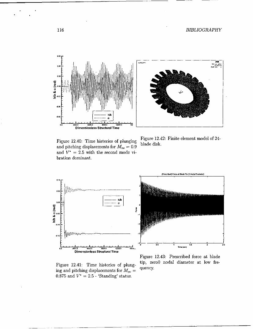
116 BIBLIOGRAPHY
AN.
0.06 Pt 0
0.03
0.
-0.03
-0.09 E0.0 3000.0 6000.0 90000 12000.0 15C
Dimensionless Structural Time
Figure 12.40: Time histories of plunging Figure 12.42: Finite element model of 24-
and pitching displacements for M.. = 0.9 blade disk.and V* = 2.5 with the second mode vi-bration dominant.
(Prescribed) Fooe at Blade Tip (0 Nodal Dianoter)
0.10
0105
-0.107
-0.10
-40 ~ ~ r~ (se1c) ' 22.
0.0 3000 6000 9000.0 '12000 15M0..
Dimensionless Structural TimeFigure 12.43: Prescribed force at blade
Figure 12.41: Time histories of plung- tip, zeroO nodal diameter at low fre-
ing and pitching displacements for Mc, = quency.0.875 and V* = 2.5 - 'Standing' status.

BIBLIOGRAPHY 117
1C1Respoes En-ofop of Blade I Tip
(Pr-iesbd) Fom at Blade Tip (0 Nodal Diameter)
3L~i
it5f
I' tl 0.2
-l I, I -02
I I v0
-2 III I -06. I
-3 -0B /
0 0005 0.01 0.015 0.02 0.025 0.03 0.030 0.04 0.045 mescTime (sec)
Figre 2.4: Pescibe foce t badeFigure 12.46: Comparison of the pre-Figuzre 12da 44: mPresribed forcfeqateblad dicted transient response at low fre-
tip eronodl dameer a lo frquecy.quency.
Response of Blade 1 Tip(Presmibod) Force at Blade Tip (D Nodal Diameler)
5.8
2 -0.6
0.4
'I It -, I'0.2-*
iI I .. 1i
-1 v '* -0.2-
-0.4
-26
-3 -0.80
________________________________________ 0 5.005 0.ý01 0.ý015 0.02 0.'25 0.03 0.035 0.04 0.045 5.052.45 2.455 2.46 2.465 2.47 2.475 2.48 2.485 2.49 2.49! Time02ec
lime (sa)
Figre 2.4: Pescibe foce t badeFigure 12.47: Comparison of the pre-
Figuzre 12.45: Prmeesribed forcfeqateblad dicted transient response at low fre-tip zeo ndaldiaete atlowfreueny.quency.

118 BIBLIOGRAPHY
4 ~~Re~pOse of Blade 1 Tip (Presebed) Forc at Blade Tip (0 Nodal Dianrter)
0.8, "
r i
'I Ii-0.24 ~ I Ij
II ~ , I I I -2 . I
-3 ifI
-0.8-'
2145 2.ý455 2.ý46 2.48 2.ý47 2.ý475 2.4'8 2.485 2.49 2.49! 0 O.00 0.02 0.003 0.004 0.005 00086 0007 0.008 0.009 0.01Tio-e(we) T-r (w0)
Figure 12.48: Comparison of the pre.- Figure 12.50: Prescribed force at bladedicted transient response at low fre- tip, zero nodal diameter at high fre-quency. quency.
(Prescried) Focme of Blade Tip (D Nodal Diamrler) (Prescrbed) Force at Blae. Tip (0 Nodal Oierrrter)
3I 3
0,,
-2-2
-3-3
0 05S 1 1.49 1.491 1.4892 1.493 1,494 1.495 1.496 1.497 1.498 1.499 1.5Tie.- (we) T.-r (ee)
Figure 12.49: Prescribed force at blade Figure 12.51: Prescribed force at bladetip, zero nodal diameter at high fre- tip, zero nodal diameter at high fre-quency. quency.

BIBLIOGRAPHY 119
Raspooo Envelop of Blade 1 Tip x 07Respooof Blade 1Tip
1.5
05 0.5-
-1.5 -1...
0 0.5 I 1.49 1.491 1.492 1.493 1.494 1.495 1.496 1.497 1.498 1.499 1.5lin~e (eon)T-n (-o)
Figure 12.52: Comparison of the pre- Figure 12.54: Comparison of the pre-dicted transient response at high fre- dicted transient response at high fre-quency. quency.
e1'Response of BladelIlip e1 ~Reponse Envelop of Blade Iip
0.5 ~ IiI .. 0.iiir
It
-1.51-,0 0.001 0.002 0003 00054 0005S 000F0 0007 0005 0.00! 0 0.5 1
Tirne (.on) lirne(en
Figure 12.53: Comparison of the pre- Figure 12.55: Comparison of the pre-dicted transient response at high fre- dicted transient response at high fre-quency. quency.
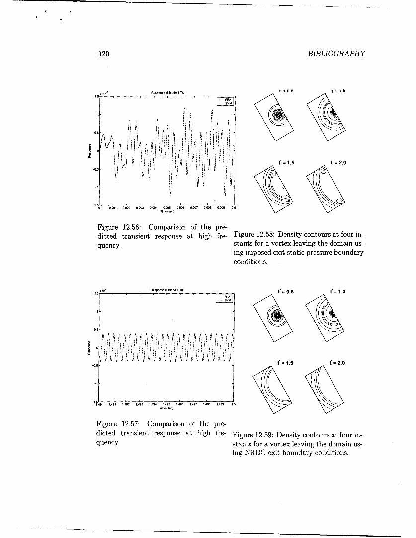
120 BIBLIOGRAPHY
r 'Respssse f BladelIT~p t=0.5 1.0
0/
I.2.0
Tke jlIw)2.
R sos ABaeI Ti 0. toI
-0
II -j J
0.4 00091 00092 00093 00094 00095 00096 00097 0.490 00009 01.T.M~ (se)
Figure 12.56: Comparison of the pre-dicted transient response at high fre- Figure 12.58: Density contours at four in-quency. stants for a vortex leaving the domain us-
conditions. buday odiios

BIBLIOGRAPHY 121
f=0.5 t=1.0
tf= 1.5 f'=2.0
•--e FPBC--- NRBC
Figure 12.60: (u" - u'U,)/u'½, contor 1at four instants for a vortex leaving t'domain using imposed exit static pressu o
boundary conditions.10.
f =0.5 t=1.0
0 5 10 15Dimensionless time
Figure 12,62: Time histories of IPrna --
Pmin [ for a vortex leaving the domain.t:1.5 t2.0
Figure 12.61: (u' - u½')/u'r, contoursat three instants for a vortex leaving thedomain using NRBC exit boundary con-ditions.
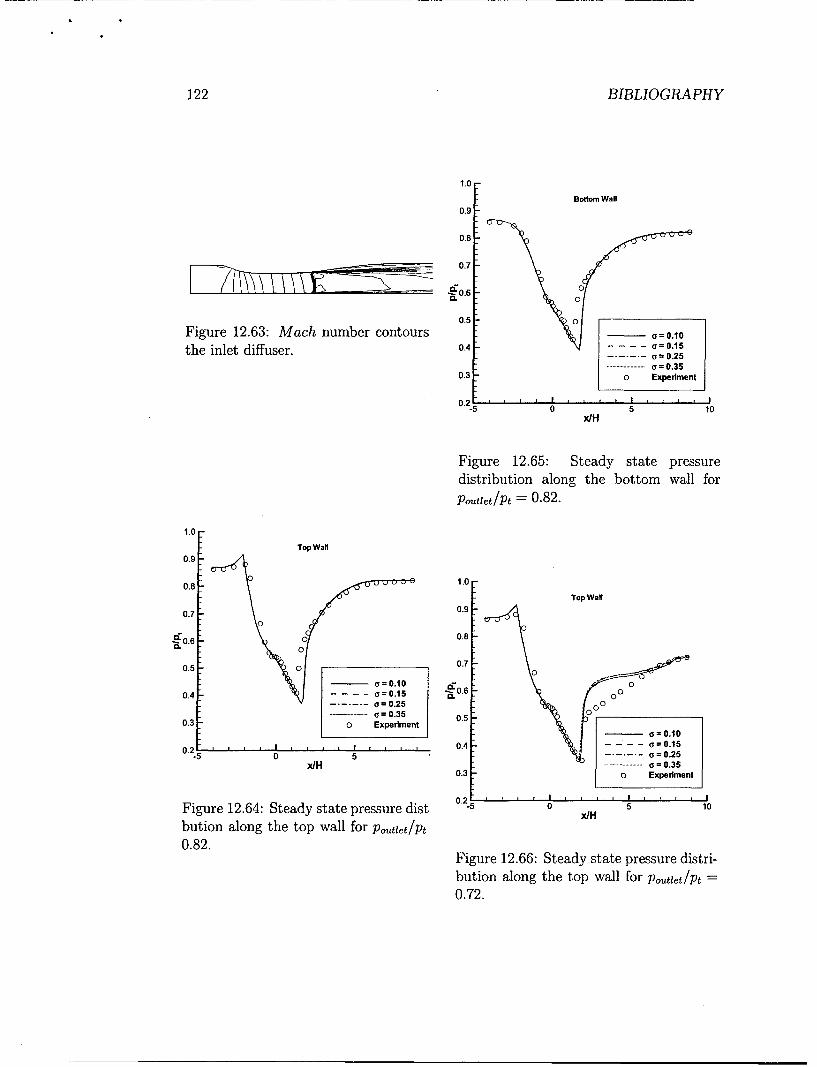
122 BIBLIOGRAPHY
1.0
Bottom wan
0.9
0.8
S 0.7
C-0.6 00
0.5 oFigure 12.63: Mach number contours _ ;=0__the inlet diffuser. 0.4..a ,2
0.3 -0 Experiment
02-5 0L . 5 . . . . 1'0x/H
Figure 12.65: Steady state pressuredistribution along the bottom wall for
=otetp 0.82.
1.07
Top Wall
0.9
0.8 UU1.0-Top Wall
0.7 0.90
060 0.8aL 0
0.5 00.0
a =0.10O0.4 - -. - - (F=O0.15 a
= .2 00
a -= 0.35 o00.3 -0 Experiment 0.5 .1
0.2 . . . . 0.4 ; 01
XIH ........a=0.350.3 -0 Experiment
02ý_Figure 12.64: Steady state pressure dist 5 0 / 51
bution along the top wall for ptei/Ptlp0.82.
Figure 12.66: Steady state pressure distri-bution along the top wall for p,,,tie /tlp0.72.

BIBLIOGRAPHY 123
1.0 1.0
Bottom Wall0.9 0.9 3 Experiment
---- FPBCNRBC, Outflow& Wall
0.8 -0.8
0.7 0.7
-0.6Cr.6 U
0. 00
0.500.
a =0.100.4 -=0.15 0.4 7Bottom Wall
-- --- a=0.250 a-..-.. = 0.35
0.3 0 Experiment 0.37
0.2 . . . . 0.2-5 0 JH 5 -5 0 xh 5 10
Figure 12.67: Steady state static pres- Figure 12.69: Time averaged unsteadysure distribution along the bottom wall pressure distribution along the bottomfor poutlet/pt 0.72. wall for Poutlet/pt 0.72.
0.9 * Experiment---- FPBC
NRBC, Outflow & Wall _____________________
0.8
0.7
-- ..
-
C0. 1
0.5 A
0.4 Top Wall
0.3 1
0.2
Figure 12.68: Time averaged unsteady Figure 12.70: Power spectral density forpressure distribution along the top wall the static pressure fluctuations at x/Hfor PutletiPt =0.72. 14.218, Poutlet/Pt =0.72.
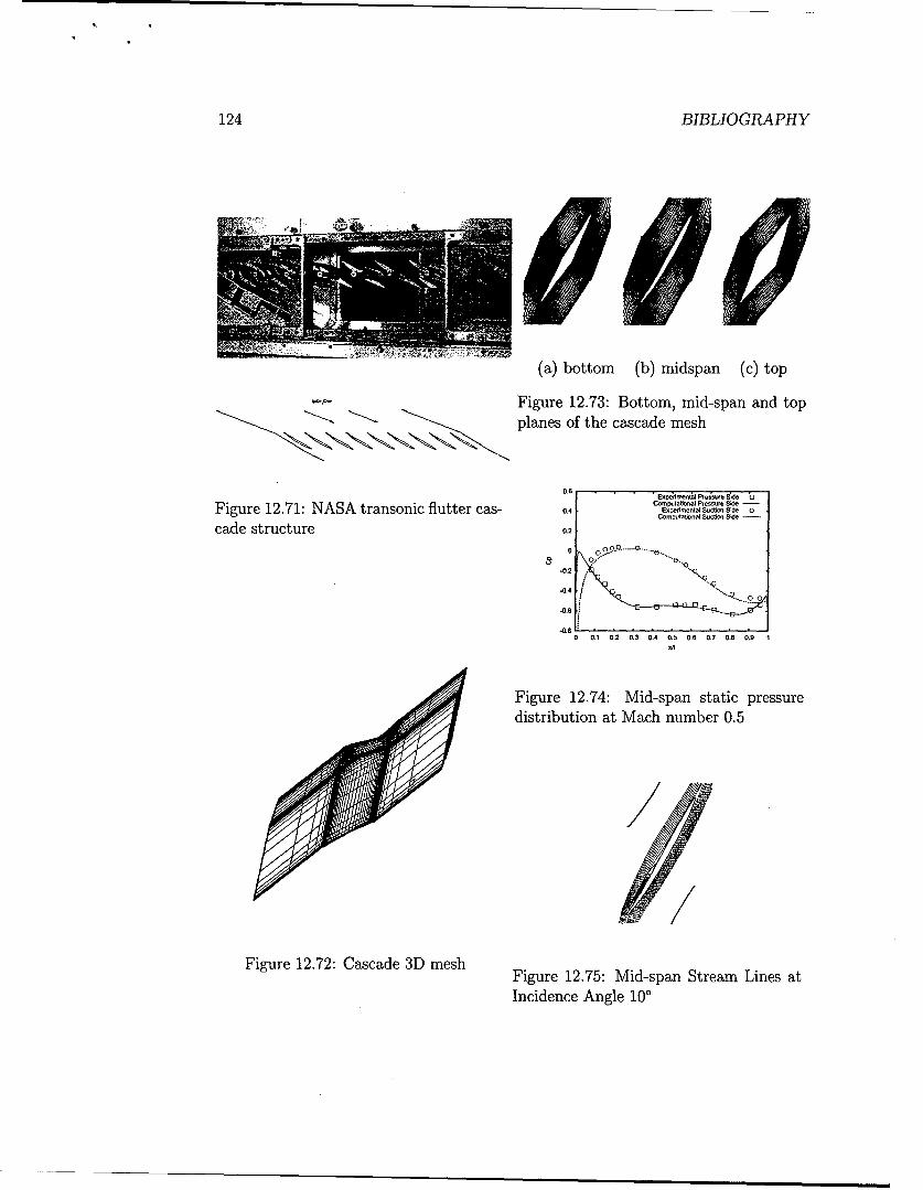
124 BIBLIOGRAPHY
(a) bottom (b) midspan (c) top
Figure 12.73: Bottom, mid-span and topplanes of the cascade mesh
0.6 . . .C~t6op in Presur. Side -.Figure 12.71: NASA transonic flutter cas- 0. C, S• ,Conu~nlSucbo Sid .....
cade structure 0.2
o .. "-. .
-0. 2 • . q
-0.4
-0.6
-0.80 0.1 0.2 0.3 0.4 0.5 0.6 0.7 0.8 0.9 1
x,1
Figure 12.74: Mid-span static pressuredistribution at Mach number 0.5
Figure 12.72: Cascade 3D mesh Figure 12.75: Mid-span Stream Lines atIncidence Angle 100

BIBLIOGRAPHY 125
Sf0.025
0.02
0.015
Figure 12.76: Mid-span Suction Surface 0.O1
Streamlines at Incidence Angle 1000.005
0.6 S0CEx.p~ermenta: PreureeSide b- 0 500 1000 1500 2000 2500 3000
Computational Pressure Side frequency (Hz)SExperimental Suction Side 0
0.4 Computational Suction Side..
0.2 0.. Figure 12.79: Separation Zone Length3 E l Variation Frequency Spectrum
0
-0.2 .//"
090-0.4 ' 11
0 0.1 0.2 0.3 0.4 0.5 0.6 0.7 0.8 0.9 1X/l
Figure 12.77: Mid-span Surface PressureDistribution at Incidence Angle 10' 2.74
2.74
2.72
2.70.8 2.68
0.75 2.66
2.640.7 2.62
0.65 2.6
2.58
0.6 2.56
2.540.55 0 5 10 15 20 25 30
t (ms)0.5
0.45
0 5 10 15 20 25 Figure 12.80: Suction Surface Checkt (ms)
Point Pressure Variation with Time
Figure 12.78: Separation Zone LengthVariation with Time
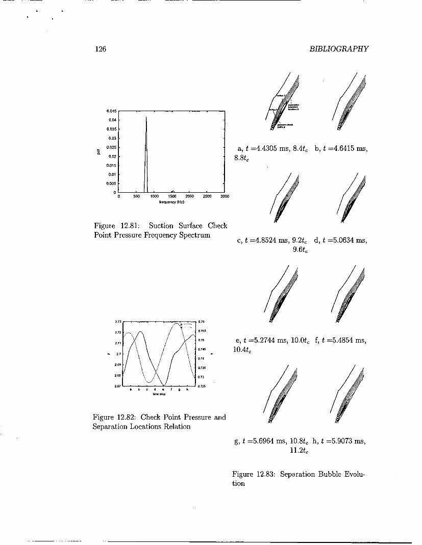
126 BIBLIOGRAPHY
0.045
0.040.035
0.03
0.0350.025 a, t =4.4305 ms, 8.4t, b, t =4.6415 ms,0.02 8.8t,
0.015
0.01
0.005
0 -
0 500 1000 1500 2000 2500 3000frequency (Hz)
Figure 12.81: Suction Surface Check
Point Pressure Frequency Spectrum c, t =4.8524 ms, 9.2t, d, t =5.0634 ms,9.6t,
2.73 . . . 0.76
2.72 .0.755
2.71 0.75 e, t =5.2744 ms, 10.0t, f, t =5.4854 ms,2.7 .745
0.742.69
0.735
2.68 0.73
267 0.725b C d e f 0 h
Figure 12.82: Check Point Pressure andSeparation Locations Relation
g, t =5.6964 ms, 10.8t, h, t =5.9073 ms,11.2t,
Figure 12.83: Separation Bubble Evolu-tion

BIBLIOGRAPHY 127
0.9 0.05
0.85 0045
0.9 0.04
0.75 0.035
0.7 0.03
0.65 0.025
0.6 0.02
0.55 0.015
0.5 0.01
0.45 0.005
0.4 00 5 10 15 20 25 0 500 1000 1500 2000 2500 3000
t(ms.) frleq nc.zy (Hz)
Figure 12.84: Separation Zone Length Os- Figure 12.87: Checkpoint Pressure Oscil-cillation (Ma=0.8) lation Frequency Spectrum (Ma=O.8)
0.45 0.285
0.4 0.28
0.350.275
0.3
0.25 0.27
0.2 0.265
0.15
0.1
0.05 0.255
0 0.250 500 1000 1500 2000 2500 3000 0 2 4 6 a 10 12
fe'.ueoy (Hz) t (.5)
Figure 12.85: Separation Zone Length Os- Figure 12.88: Checkpoint Pressure Oscil-cillation Frequency Spectrum (Ma=O.8) lation (Ma=1.18)
1.06 1.068&06
1.04
1.02 6e-06
1 4.06O0"918 !2e-064e0
0.96
0.94 00 5 10 15 20 25 0 500 Iw0 1 20 200 2500 3000
t (m) *05keque. Hz)
Figure 12.86: Checkpoint Pressure Oscil- Figure 12.89: Checkpoint Pressure Oscil-lation (Ma=0.8) lation Frequency Spectrum (Ma=l.18)

128 BIBLIOGRAPHY
P, P, P3 It p, P. P P, PtI
'57Zs57 fz1 t-*
Blade Incidence (degree)
0.03
0.02 - 3Figure 12.90: Cascade structure and CFD o.01
setup .01 ,,
-0.02
-0.03
Pressure Oscillation on Lower Surface
0.15
-0.1
Pressure Oscillation on Upper Surface
Figure 12.91: Cascade Mesh 0.1 i..'--.. ... .• . ..•...0.05 r .•' • • " x/c-o.5 ........ . ...
0 1 2 3 4 5 6 7 A 9
Time (ms)
Figure 12.94: Pressure oscillation at dif-ferent chordwise locations
Figure 12.92: Additional mesh layer forbetter orthogonality
2.2-W.. . '.,ii!:• . . . ., t.
0 ..... .. . Figure 12.95: Mach number contours ofthe cascade
Figure 12.93: Pressure oscillation history
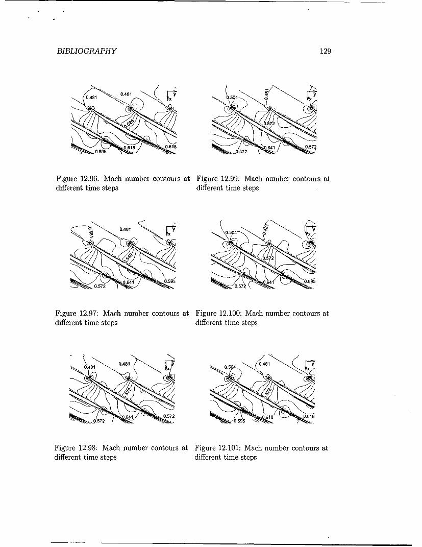
BIBLIOGRAPHY 129
0.5955o72
Figure 12.96: Mach number contours at Figure 12.99: Mach number contours atdifferent time steps different time steps
OV4 0.504
Figure 12.97: Mach number contours at Figure 12.100: Mach number contours atdifferent time steps different time steps
Figure 12.98: Mach number contours at Figure 12.101: Mach number contours atdifferent time steps different time steps

130 BIBLIOGRAPHY
0o.481 F
0. 4 0.9'5.0.2
Figure 12.102: Mach number contours at 0.6 8
different time steps
Figure 12.105: Mach number contours at01N different time steps
15•
Figure 12.103: Mach number contours at -,
different time steps ..1
0 0.1 0.2 0.3 04 0. 0,1 0.7 0. 0.91
Figure 12.106: Unsteady pressure analy-
Figure 12.104: Mach number contours at sisdifferent time steps

BIBLIOGRAPHY 131
-0.2
Figure 12.107: Computation Domain - was
Configuration0 0,2 0A4 01 8
Figure 12.110: Steady state pressure co-efficient in 2-passage cascade
Figure 12.108: Computation mesh ; ___,___,_____12___"____,___
0 5 10 15 20 25 30 35 40
us - LS.
Thme (ms)
Figure 12.111: Pressure oscillation his-tory, k,= 0.8
'N~l0
0
~~ US '. ~~~0 01 0 03 0 05 6 0. 0 00
CFD
F 0f0o
L -us 0 0.1 02 o03 0A 0,5 0A 0.7 01• 01
Figure 12.112: Unsteady pressure coeffi-cient on upper surface in 2-passage cas-
Figure 12.109: Two-passage cascade peri- cade, k, 0.8odic computation domain
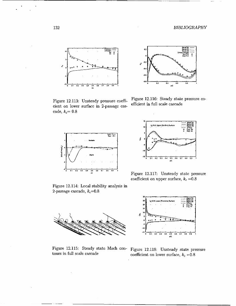
132 BIBLIOGRAPHY
CFD'•BC)~ ~ --- Blde B4 -
•0 k "C" CDep ... 2 Blade B5 -toCF 'BBýjBlade B6 ...
m 01 . .. ... x r
0 0 0 0 0 0 0 if
.0.4
o0 0 0.2 003 0.4 0.5 06 07 08 0.0 sC
5k
Figure 12.113: Unsteady pressure coeffi- Figure 12.116: Steady state pressure co-
cient on lower surface in 2-passage cas- efficient in full scale cascade
cade, k,= 0.8
-- Blade B50 kc=0.8, Upper I(Suc~n) Sudace ...... Slade B6
0 .00. ....... 2-P. s0 E00 0 Re0 Exp. 1m
CFOc20 .- .oel. ........ ... ....
0 ~
15 -15
0 0.1 0.2 0.3 0.4 0.5 0.6 0.7 0.8 0.9 1
x/C
-3 0, t O2 0,3 A0. 5 . 0,6 07 0.a 01
"FS sFigure 12.117: Unsteady state pressurecoefficient on upper surface, k, =0.8
Figure 12.114: Local stability analysis in2-passage cascade, kc.=0.8
25 k-,O.S. Lowr(P -su) Surface - .. Blade B5
20 .. . . xp. Re0 Or0 00 0 o e ""0 {•:2-:
-15
• .0 . 0. O2 0.3 0.4 0.5 0.6 0.7 0.8 0.9 1
Figure 12.115: Steady state Mach con- Figure 12.118: Unsteady state pressuretours in full scale cascade coefficient on lower surface, k, =0.8
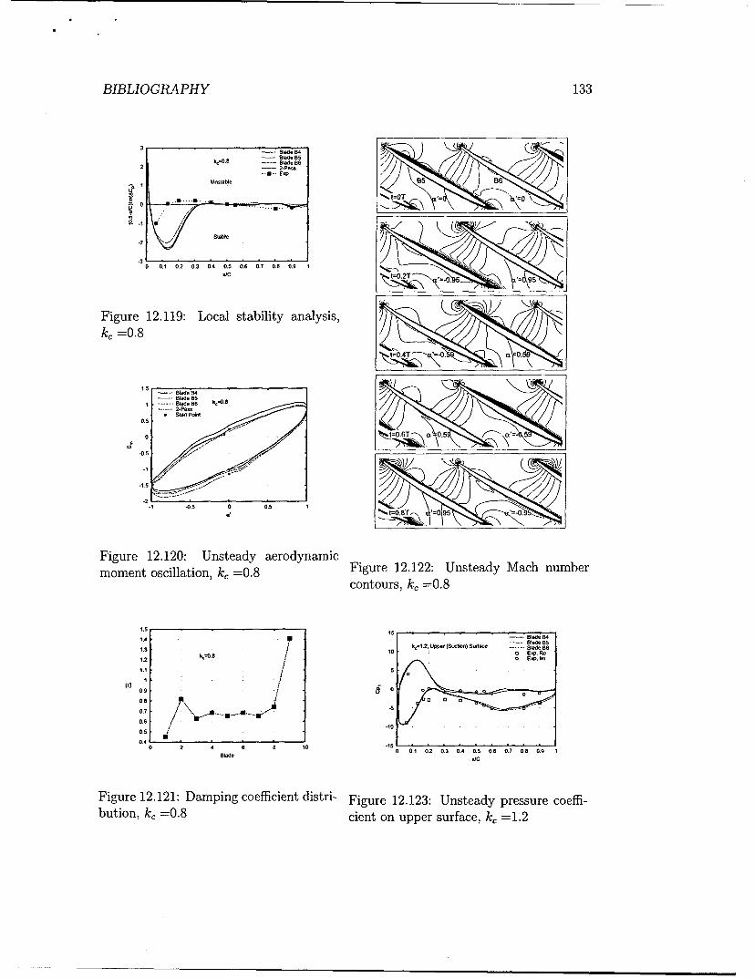
BIBLIOGRAPHY 133
k0.8 - Bb'e 152 ... Blade B6
- UnStable
.2 Y'
"0 0.1 02 0.3 04 0.5 0.6 0.7 0. 0.9 1
Figure 12.119: Local stability analysis,k , =0.8
-tt=A -'=0 ,0
S-- Blade 84
Bl.a....Bde B6 • . S...... 2.Pass• Stant Point
-0.5
~306 '0.5 5
-2. -0.5 0 0.5 1 /1-OS • I=15",.' " " =.•• ,,' ,Ce t-0.8T 50 95_
Figure 12.120: Unsteady aerodynamicmoment oscillation, k, =0.8 Figure 12.122: Unsteady Mach numbercontours, kc =0.8
1.5 15 | -- B_ _e B4
1.4 - BUle B4
1.3 1 ltI1.2. Upper (SM on) Surface ------ Blde 061. k,0.8o a 0 Exp, R1.2 1.
1.1 I 0
hi|
0.9
0.8I
0.6 / "-10- •
0.5
40 2 4 Blade 6 a 150 0.1 0.2 0.3 0.4 0.5 0.6 0.7 0.8 0.9
1/C
Figure 12.121: Damping coefficient distri- Figure 12.123: Unsteady pressure coeffi-bution, k, =0.8 cient on upper surface, k, =1.2

134 BIBLIOGRAPHY
25 ) - Blade B4t 2.5 -- Blade 04
20 k•1.2. Lo (Pressure) Su.rce ade2 kB,4 -- 8ladeB5
. lade B6 2 B0lde B6exp,' . Re •M1. Exp
0 15 02 03 04 00 0 0) 0.0 .9 ¶r 1.5
0 01 0 U0stable
cin n oe c.cae k o Exp.2 kh0.4
-- 41.1
50.5
-10
-15 .1
0 0.1 0.2 0.3 0.4 0.5 0.6 0.7 0.6 0.9 1 0-2 6 8 1
WC 0 0.1 0.2 0.3 0O4 0.5 0.6 0.7 0. . 9
Figure 12.124: Unsteady pressure coeffi- Figure 12.127: Local stability analysis,cient on lower cascade, k, =1.2 k0 =0.4
3 1-- Blade BA2 - Blade B5
.. Blade B6
S ....•kE 0.0 * kt + 50 4 / "
1. o .7. A /1.2 . 0.9
0.0.•
0.7 -1.7
0. -0.3
631S.bl 0. .. .
-5 , , 0.2 , ,
0 0.1 0.2 0.3 0.4 0.5 0.6 0.7 0.8 0.921 4 6 8 1
VtC Blade
Figure 12.125: Local stability analysis, Figure 12.128: Damping coefficient distri-kb =1.2 bution, ko =0.4
1.61 c J
S;kC-0.4 Blade 85
S• 0
0,8
0A 0 -.. .5m
0.5 'L -
0 2 4 6 a 10 -1 -0.5 0 0.5
Blade a
Figure 12.126: Damping coefficient distri- Figure 12.129: Unsteady aerodynamic
bution, k, =1.2 moment oscillation comparison

BIBLIOGRAPHY 135
InFg ral flow field and structuralw1•1., 0", S"
FgCrD,e 1CFDk=. 8 --l2CFD. C12...
Exp. k,-0.8 .I.
strExp.ek1.2 intertodyn caic u o p
., ,, ............. S ucu !d~tc me t I •
eby= structure
I In
70
-3CFD movin and deorng it
0.1 0.2 0.3 11.. 0.5 0.6 0.7 0.8 0.9 1h
C arDflowedldbybooang
flow govewnin equatsora
Figure 12.130: Local stability analysiscomparison u•••7• ....
Figure 12.132: Fully coupled flow-structure interaction calculation proce-dure
80 J -
60
50'
>, 40 •,// Far-field boundary
10 dy,;--~
NOw wing surface
10 J~ €•x• L~X•'• Old wing surface
0 C . . . I A . . . .
20 40 60x
Figure 12.131: A sketch of the mesh dformation
Figure 12.133: The mesh around the ON-ERA M6 wing surface.
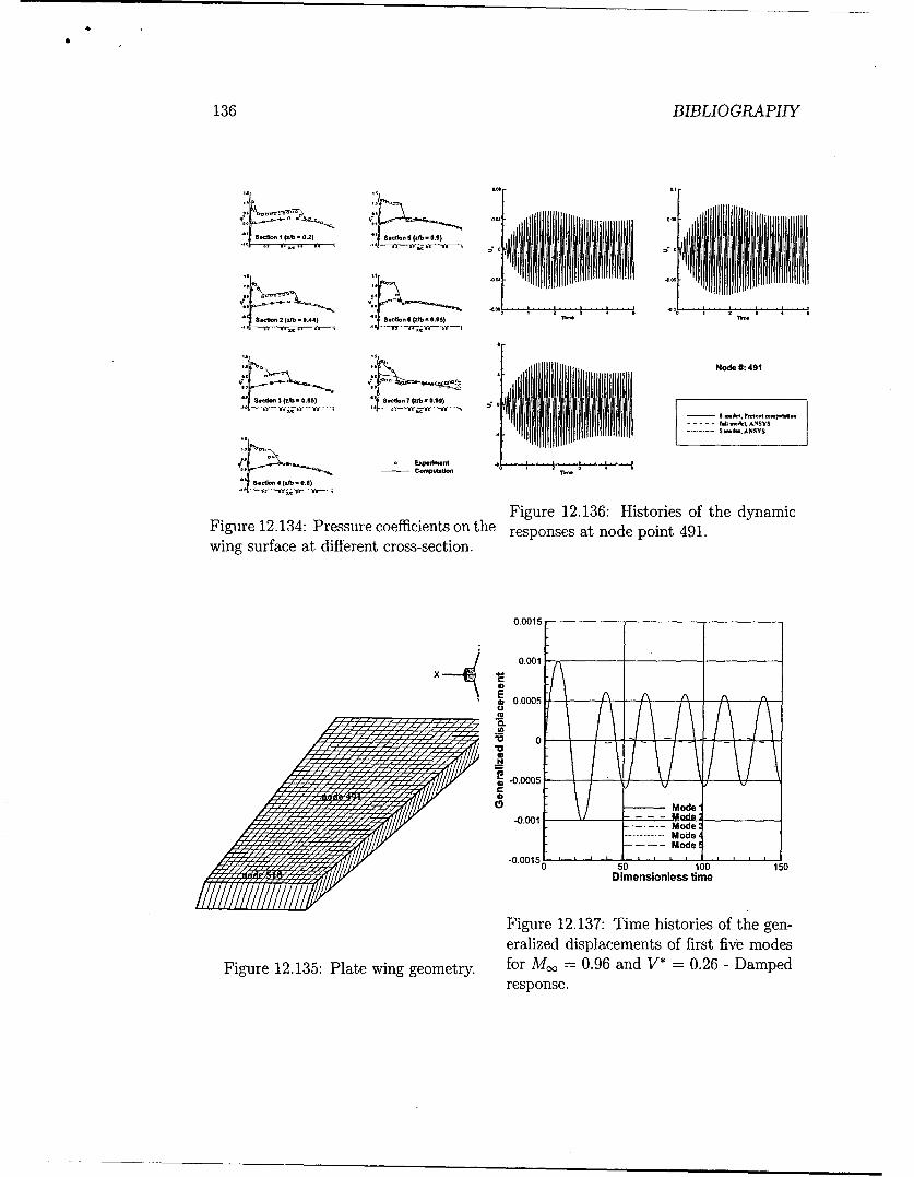
-bS
136 BIBLIOGRAPHY
.. . . . . . . . . .... .
5.tiooibO.jSedin S •o -o.g.) Iq•o
4 .• ctd 3 (zvb D.805) •eISecon i7 (M~ 0.95)Tn ie
----- --- SmdII, ,,,
0 .0 0150 0 2 0
N.. .oi;rde, #A 491
0.001 .0..,ro~oooooo.
x 0 do., ANSYS
04 s0
-0.0 (sibn* r.3)
Figure 12.136: Histories of the dynamicFigure 12.134: Pressure coefficients on the rsossa oepit41
0epne Mtnd ode 41
wing surface at different cross-section.
0.0015
.0 .0 0 1 L U L -
S5 0.0005
-_o:
eralize diplcmet Mofdestf- oe
-0.001 . . od
O...-.Mode
...................................................... Mode,.. .Mode
-0,00150 50 100 150
Dimensionless time
Figure 12.137: Time histories of the gen-eralized displacements of first five modes
Figure 12.135: Plate wing geometry. for M, = 0.96 and V* = 0.26 - Dampedresponse.

BIBLIOGRAPHY 137
0.0015
0.001
E
V
V _ A [ A
(.9 -- Mode.0.0011 . .. Mode,
S.. . . Mode: S......... M ode. . Mode! 0.6
-0.00150 ,.. . . . , , ,,050 100Dimensionless time O Present computation
-- B-- Experiment
0.5
Figure 12.138: Time histories of the ge 'm 0
eralized displacements of first five rood .•_ýstable response.o
U.m0.30 5
00.0015M
-0.0015..L J..... '............ .L......I.....
0.001 0..2 0.4 0.6 U. 1 1.2 1.4-- Mach NumberE A00.0005
Fiur Figure 12.140: Comparison of predicted
' 0 h . .I- I wing flutter boundary with experimentale data for AGARD Wing 445.6.
fo-M0. 0.6an0V050.8 -VNurl&.
saerpMode's-0.001 . Mode
--.. --- Mode.................. M ode ,
.. .Mode-0.0015.
50 100 150
Dimensionless time
Figure 12.139: Time histories of the gen-eralized displacements of first five modesfor M,, = 0.96 and V* = 0.315 - Diverging
response.