AFRL-RZ-WP-TR-2010-2132

POWER AND THERMAL TECHNOLOGIES FOR AIR AND SPACE‒SCIENTIFIC RESEARCH PROGRAM Delivery Order 0017: Study of Microchip Power Module Materials Using Mini-Channel Heat Exchanger Andrew Cole and Jamie Ervin University of Dayton Research Institute (UDRI) Larry Byrd Thermal and Electrochemical Branch Energy/Power/Thermal Division

DECEMBER 2009 Interim Report

Approved for public release; distribution unlimited. See additional restrictions described on inside pages

STINFO COPY

AIR FORCE RESEARCH LABORATORY PROPULSION DIRECTORATE

WRIGHT-PATTERSON AIR FORCE BASE, OH 45433-7251 AIR FORCE MATERIEL COMMAND

UNITED STATES AIR FORCE

NOTICE AND SIGNATURE PAGE Using Government drawings, specifications, or other data included in this document for any purpose other than Government procurement does not in any way obligate the U.S. Government. The fact that the Government formulated or supplied the drawings, specifications, or other data does not license the holder or any other person or corporation; or convey any rights or permission to manufacture, use, or sell any patented invention that may relate to them. This report was cleared for public release by the USAF 88th Air Base Wing (88 ABW) Public Affairs (AFRL/PA) Office and is available to the general public, including foreign nationals. Copies may be obtained from the Defense Technical Information Center (DTIC) (http://www.dtic.mil). AFRL-RZ-WP-TR-2010-2132 HAS BEEN REVIEWED AND IS APPROVED FOR PUBLICATION IN ACCORDANCE WITH THE ASSIGNED DISTRIBUTION STATEMENT. *//Signature// //Signature//

TRAVIS MICHALAK THOMAS L. REITZ Program Manager Chief, Thermal and Electrochemical Branch Thermal and Electrochemical Branch Energy/Power/Thermal Division Energy/Power/Thermal Division Propulsion Directorate Propulsion Directorate This report is published in the interest of scientific and technical information exchange, and its publication does not constitute the Government’s approval or disapproval of its ideas or findings. *Disseminated copies will show “//Signature//” stamped or typed above the signature blocks.

REPORT DOCUMENTATION PAGE Form Approved

OMB No. 0704-0188

The public reporting burden for this collection of information is estimated to average 1 hour per response, including the time for reviewing instructions, searching existing data sources, gathering and maintaining the data needed, and completing and reviewing the collection of information. Send comments regarding this burden estimate or any other aspect of this collection of information, including suggestions for reducing this burden, to Department of Defense, Washington Headquarters Services, Directorate for Information Operations and Reports (0704-0188), 1215 Jefferson Davis Highway, Suite 1204, Arlington, VA 22202-4302. Respondents should be aware that notwithstanding any other provision of law, no person shall be subject to any penalty for failing to comply with a collection of information if it does not display a currently valid OMB control number. PLEASE DO NOT RETURN YOUR FORM TO THE ABOVE ADDRESS.

1. REPORT DATE (DD-MM-YY) 2. REPORT TYPE 3. DATES COVERED (From - To)

December 2009 Interim 05 May 2008 – 10 December 2009 4. TITLE AND SUBTITLE

POWER AND THERMAL TECHNOLOGIES FOR AIR AND SPACE‒SCIENTIFIC RESEARCH PROGRAM Delivery Order 0017: Study of Microchip Power Module Materials Using Mini-Channel Heat Exchanger

5a. CONTRACT NUMBER

FA8650-04-D-2403-0017 5b. GRANT NUMBER

5c. PROGRAM ELEMENT NUMBER

62203F 6. AUTHOR(S)

Andrew Cole and Jamie Ervin (University of Dayton Research Institute (UDRI)) Larry Byrd (AFRL/RZPS)

5d. PROJECT NUMBER

3145 5e. TASK NUMBER

S3 5f. WORK UNIT NUMBER

3145S300 7. PERFORMING ORGANIZATION NAME(S) AND ADDRESS(ES) 8. PERFORMING ORGANIZATION

University of Dayton Research Institute (UDRI) 300 College Park Dayton, OH 45469-0145

Thermal and Electrochemical Branch (AFRL/RZPS) Energy/Power/Thermal Division Air Force Research Laboratory, Propulsion Directorate Wright-Patterson Air Force Base, OH 45433-7251 Air Force Materiel Command, United States Air Force

REPORT NUMBER

9. SPONSORING/MONITORING AGENCY NAME(S) AND ADDRESS(ES) 10. SPONSORING/MONITORING AGENCY ACRONYM(S)

Air Force Research Laboratory Propulsion Directorate Wright-Patterson Air Force Base, OH 45433-7251 Air Force Materiel Command United States Air Force

AFRL/RZPS 11. SPONSORING/MONITORING AGENCY REPORT NUMBER(S)

AFRL-RZ-WP-TR-2010-2132

12. DISTRIBUTION/AVAILABILITY STATEMENT

Approved for public release; distribution unlimited.

13. SUPPLEMENTARY NOTES

PAO Case Number: 88ABW-2010-2009, Clearance Date: 13 Apr 2010. Report contains color.

14. ABSTRACT An apparatus to simulate the cooling of a silicon carbide (SiC) metal oxide semiconductor field excited transistor (MOSFET) using a mini-channel heat exchanger with a single phase (liquid) fluid was constructed. The chip was simulated with a sample of SiC that is heated on one surface and cooled on the opposing surface using a mini-channel heat exchanger. One goal of this work was to demonstrate that the apparatus has the capability to remove a heat flux of 100 W/cm2 from the surrogate chip while maintaining its temperature below 200 °C. A second goal was to characterize the thermal and flow behavior of the mini-channel heat exchanger for different flow rates and heat fluxes by experiments and numerical simulation using computational fluid dynamics. The maximum heat flux removed by the mini-channel heat exchanger was 110 to 117 W/cm2 with a maximum stem temperature of 112 °C at the interface. The NuD values determined here were in the range of 9 to 23, which agree reasonably well existing with convective heat transfer correlations. For flows up to a ReD of 3600, there was good agreement with the theoretical pressure loss. Lastly, computational fluid dynamics simulations provided insight into the effect of the heated length on NuD estimates and flow and convective heat transfer behavior.

15. SUBJECT TERMS

SiC MOSFET, heat flux, mini-channel heat exchanger

16. SECURITY CLASSIFICATION OF: 17. LIMITATION OF ABSTRACT:

SAR

18. NUMBER OF PAGES

106

19a. NAME OF RESPONSIBLE PERSON (Monitor)

a. REPORT Unclassified

b. ABSTRACT Unclassified

c. THIS PAGE Unclassified

Travis E. Michalak 19b. TELEPHONE NUMBER (Include Area Code)

N/A

Standard Form 298 (Rev. 8-98) Prescribed by ANSI Std. Z39-18

i

Table of Contents Section Page

List of Figures ................................................................................................................................. ii List of Tables ................................................................................................................................. iv

1. Summary .............................................................................................................................. 1

2. Introduction .......................................................................................................................... 2

3. Experimental description ...................................................................................................... 5

3.1 Test Stand .......................................................................................................................... 7 3.1.1 Copper Heater Block .............................................................................................. 10

3.1.2 The Heat Exchanger ............................................................................................... 11

3.1.3 Alignment Stand ..................................................................................................... 15

3.1.4 Glas-Therm Block .................................................................................................. 17

3.1.5 Load Apparatus ...................................................................................................... 18

3.1.6 Test Stand Insulation and Heat Loss Reduction ..................................................... 19

3.1.7 Water Chiller .......................................................................................................... 20

3.2 Instrumentation ................................................................................................................ 22

3.2.1 Thermocouples ....................................................................................................... 22

3.2.2 Load Measurement ................................................................................................. 25

3.2.3 Pressure Transducers .............................................................................................. 25

3.2.4 Mass Flow Rate ...................................................................................................... 26

3.2.5 Electrical Supply Components ............................................................................... 27

4. Experimental Procedure ..................................................................................................... 30

4.1 Water Chiller ................................................................................................................... 30

4.2 Pressure and Flow Rate ................................................................................................... 32

4.3 Contact Load ................................................................................................................... 32

4.4 Power Supplies ................................................................................................................ 32

5. Results and Discussion ....................................................................................................... 33

5.1 Conduction Heat Transfer through Copper Stem ............................................................ 33

5.2 Convective Heat Transfer within Mini-Channel Heat Exchanger .................................. 38

5.2.1 Numerical Analysis ................................................................................................ 38

5.2.2 Comparison with Experimental Data ..................................................................... 45

6. Flow Characterization ........................................................................................................ 52

6.1 Head Loss ........................................................................................................................ 52

6.2 Characterization of the Channels – Pressure Loss .......................................................... 56

7. Contact Resistance ............................................................................................................. 63

8. Conclusions ........................................................................................................................ 65

9. References .......................................................................................................................... 66

Appendix A Sample Calculations ................................................................................................. 72

Appendix B Uncertainty Analysis ................................................................................................ 75

Appendix C Calibration Methods ................................................................................................. 81

Appendix D System Diagrams...................................................................................................... 89

Appendix E Wiring Schematic ..................................................................................................... 90

Appendix F LabView Data Acquisition Program ......................................................................... 91

Appendix G Copper Material Quantification (EDAX) ................................................................. 93

NOMENCLATURE ..................................................................................................................... 94

ii

LIST OF FIGURES Figure Page

Figure 1. Schematic of Test Cell ..................................................................................................... 6

Figure 2. Experimental Electronics Cooling Apparatus ................................................................. 7

Figure 3. The First Test Stand......................................................................................................... 8

Figure 4. The Second Test Stand .................................................................................................... 9

Figure 5. Section Drawing of the Test Stand ................................................................................ 10

Figure 6. Sectioned Copper Heater Block .................................................................................... 11

Figure 7. An Image (a) and a Drawing (b) of the Mini-Channel Heat Exchanger ....................... 12

Figure 8. Angled (a) and Front (b) View of the Mini-Channel Heat Exchanger .......................... 13

Figure 9. Two Halves of the Mixing Chamber and the Inlet (or Exit) of the Flow Tube ............. 15

Figure 10. Top (a) and Bottom (b) Views of the Upper Alignment Plate .................................... 16

Figure 11. Glas-Therm Block with Respect to Tubing (a) and Upper Alignment Plate (b) ......... 17

Figure 12. Apparatus for Imposing Repeatable Thermal Load on the Copper Stem and Heat Exchanger ..................................................................................................................................... 18

Figure 13. Insulated Copper Block and Convection Shield Surrounding the Test Stand ............. 19

Figure 14. Chiller/Pump (a) for Cooling and Flow with Valve (b) for Pressure Adjustment ...... 20

Figure 15. Two Valves for Gross and Fine Flow Adjustment ...................................................... 21

Figure 16. Inlet (or Exit) Flow Thermocouple with Pressure Port in the Bottom of the Four-Way Fitting ............................................................................................................................................ 22

Figure 17. Thermocouples (Circled) Attached to the Sides of the Stem ...................................... 23

Figure 18. Location and Position References for the Stem Thermocouples ................................. 24

Figure 19. Stress Relief Clamps for Heater Thermocouples ........................................................ 24

Figure 20. Load Apparatus and Load Cell on the Upper Alignment Plate ................................... 25

Figure 21. Pressure Transducer in Front of the Test Stand ........................................................... 26

Figure 22. Flow Meter with Transmitter ....................................................................................... 27

Figure 23. Schematic of the Voltage Divider Installed for the Load Cell Circuit ........................ 27

Figure 24. Power Supply for Pressure Transducer, Flow Meter, and Load Cell .......................... 28

Figure 25. Power Supply for the Cylindrical Heater within the Copper Heater Block ................ 28

Figure 26. Cylindrical Heater Located within the Copper Block (on the Right) .......................... 29

Figure 27. Schematic of the Capacitors Connected to the Heater ................................................ 29

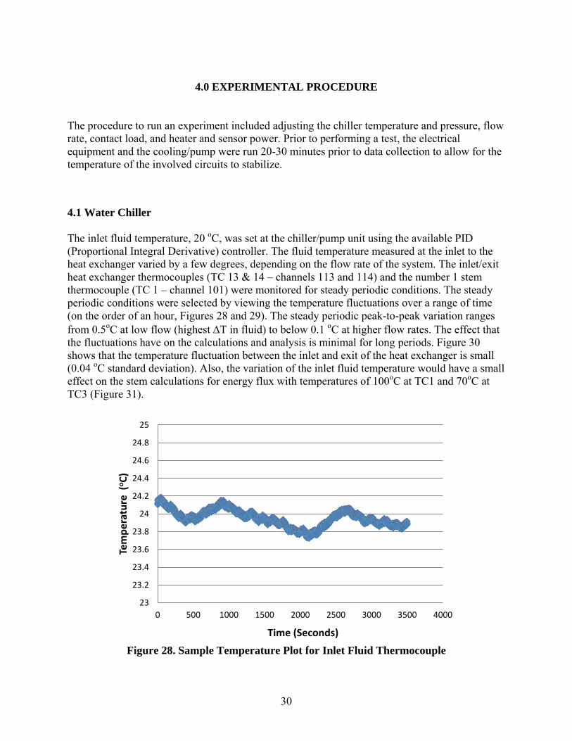
Figure 28. Sample Temperature Plot for Inlet Fluid Thermocouple ............................................ 30

Figure 29. Sample Stem Temperature Trend (Thermocouple #1, Same Test as in Figure 28) .... 31

Figure 30. Temperature Difference between Inlet and Exit of Heat Exchanger .......................... 31

Figure 31. Six Thermocouple Positions on Copper Stem (Upper Portion of Heater Block) ........ 33

Figure 32. Temperature Distribution along Copper Stem for Water Flow Rate of 7g/s .............. 34

Figure 33. Stem Temperature Profile ( ±0.005 in Thermocouple Placement) .............................. 36

Figure 34. Sketch of Expected Heat Conduction Flux Directions within the Stem ..................... 36

Figure 35. Energy Balance: Stem Conduction and Enthalpy Rise of Water ................................ 37

Figure 36. Heat Transfer Rate to the Eleven Channels of the Heat Exchanger ............................ 39

Figure 37. Calculated Temperatures (K) inside and outside the Center Channel (ReD of 1260) . 40

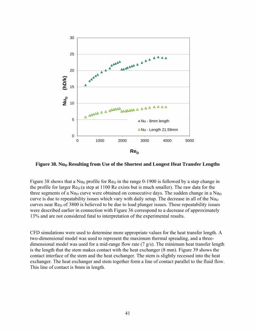
Figure 38. NuD Resulting from Use of the Shortest and Longest Heat Transfer Lengths ............ 41

Figure 39. The Heat Exchanger and Stem Form a Line of Contact Parallel to Fluid Flow .......... 42

Figure 40. Temperature Contour Plot for a Two-Dimensional CFD Solution (ReD of 1260) ...... 42

iii

Figure 41. Two-Dimensional Temperature Contours (from Three-Dimensional Model) along the Channel Centerline (ReD of 1260) ................................................................................................ 43

Figure 42. Comparison of Three Characteristic Heat Transfer Lengths ....................................... 44

Figure 43. NuD (Shah (1978)) Correlation for Combined Thermal and Hydrodynamic Entrance Length with NuD Determined from Experimental Measurements (L = 21.59 mm) ..................... 46

Figure 44. NuD Derived from the Churchill and Ozoe Correlation (1973) Plotted with Measured Values ........................................................................................................................................... 48

Figure 45. Comparison of Shah and London (1978) Uniform Heat Flux Correlation with Experimental Data ........................................................................................................................ 49

Figure 46. Comparison of Experimental Data with a Correlation for Entry Flow with Constant Surface Temperature (Kakac et al., 1987) .................................................................................... 50

Figure 47. Comparison of All Correlations with Experimentally Determined NuD ..................... 51

Figure 48. Sectional View of Heat Exchanger Showing the Flow Path ....................................... 52

Figure 49. Head Loss Values (Idelchik, 1986) Plotted with ReD for Each Flow Situation .......... 54

Figure 50. Measured P across the Heat Exchanger, Measured P Minus the P from Head Loss Calculations, and the P Given by the Poiseuille Equation ......................................................... 57

Figure 51. SEM Images of (a) a Single and (b) Multiple Channels ............................................. 58

Figure 52. Comparison of Experimental Friction Factor with and without Head Loss from Accessory Fittings to the Darcy Friction Factor for Hagen-Poiseuille Flow (White, 1974) ........ 59

Figure 53. Comparison of Experimental Friction Factor without Head Loss to that of Ghajar et. al (2008), Hagen-Poiseuille Flow (White, 1974) , and Blausius (White, 1974). .......................... 60

Figure 54. Significant Change in the Flow Near a ReD of 3600 Indicated by the Upward Bend in the Friction Factor Curve .............................................................................................................. 61

Figure 55. Rate of Enthalpy Rise for the Cooling Fluid with and without Thermal Grease ........ 63

Figure 56. Heat Transfer Rate through the Copper Stem with and without Thermal Grease ....... 64

iv

LIST OF TABLES Table Page

Table 1. Equations (Idelchik, 1986) Used to Calculate Loss Coefficients for a Particular Flow Event Neglecting fr (Minor Loss Coefficient) ............................................................................. 55

Table C-1. Curve Fits for Thermocouples 1-12 (Stem, Body, and Chamber) .............................. 84

Table F-1. Channel Locations in Agilent DAQ Unit for Each Experimental Instrument ............ 91

Table F-1. Channel Locations in Agilent DAQ Unit for Each Experimental Instrument ............ 91

1

1.0 SUMMARY

In response to a request from Dr. Jim Scofield of RZPE, the RZPS thermal group constructed an apparatus to simulate the cooling of a silicon carbide (SiC) MOSFET using a mini-channel heat exchanger with a single phase (liquid) working fluid. The chip was simulated with a sample of SiC that is heated on one surface and cooled on the opposing surface using a mini-channel heat exchanger. One goal of this work was to demonstrate that the apparatus has the capability to remove a heat flux of 100W/cm2 from the surrogate chip while maintaining its temperature below 200oC. A second goal was to characterize the thermal and flow behavior of the mini-channel heat exchanger for different flow rates and heat fluxes by experiments and numerical simulation using computational fluid dynamics. This work is part of a longer term Air Force program which has multiple projects seeking to find the optimum electronic module package. The fabricated test stand and heat exchanger showed relatively good effectiveness in transferring thermal energy. In the experiments, the maximum heat flux removed by the mini-channel heat exchanger was 110-117 W/cm2 with a maximum stem temperature of 112oC at the interface. The NuD values determined here were in the range of 9-23, which followed several heat transfer correlations reasonably well. For flows up to a ReD of 3600, there was good agreement with the theoretical pressure loss. The transition to turbulent flow at a ReD of 3600 for the present experiments is greater (by 1000) than many other works reviewed and is likely due to the very low surface roughness of the channels (0.2 m). Lastly, computational fluid dynamics simulations provided insight into the effect of the heated length on Nusselt number estimates and flow and convective heat transfer behavior.

2

2.0 INTRODUCTION

The demand for higher flight speeds, more power-dense avionics, and advanced weaponry is limited by aircraft weight and thermal restrictions. The Air Force More Electric Aircraft Initiative has the goal of using improved electronic technology to replace heavy mechanical systems which tax the energy generation of power plants and may have relatively high maintenance costs. For example, using electrical actuation rather than hydraulic actuation eliminates complex piping, mechanical components, and the need for hydraulic fluid. However, the replacement of traditional aircraft mechanical systems which use well-established cooling methods with electrical systems which use advanced cooling methods and materials are active areas of research. One approach to the thermal management of electronic circuits is to increase the allowable operating temperature by the development of new materials, such as SiC.

The use of SiC to fabricate electronic components offers advantages over the use of Si which has been used in electronic components for decades. Moreover, new aircraft electronic components will have more stringent performance requirements than those of the past. SiC offers higher temperature limits (200-250oC) for electronic components relative to those which use Si (temperature limits in the range 125-150oC). In addition, the upper temperature limit for SiC components is expected to reach 600oC (for wind turbines and hybrid energy generation) which will drive future research and development (Marckx, 2006). In the use of high-voltage electronic devices, the breakdown voltage (voltage at which electrons begin unwanted travel across interfaces) is an important characteristic to consider. SiC has a much higher breakdown voltage (~3MV/cm) than Si (0.6 MV/cm) which allows SiC devices to have relatively high operating voltages and small dimensions without power leakage to surrounding elements (Ozpineci, 2007). Small devices are often necessary for space-constrained environments. Currently, only a few SiC devices exist which include the junction field effect transistor (JFET) and Schottky diode. However, these are hybrid devices comprised of Si insulated gate bipolar transistors (IGBT‟s) and SiC switching components. Metal oxide semiconductor field excited transistor (MOSFET) devices are the future of SiC devices with release possible for the near future (Hasanuzzaman, 2004). MOSFET devices do not require a voltage to switch off (unlike a JFET), and high frequency capabilities (greater than 100 kHz) are capable with low internal capacitance which reduces full on-off time and electrical loss (Bontemps, 2007).

Unfortunately, the use of SiC as a MOSFET device has drawbacks because of technology limits with cooling and power connections. Presently, the use of SiC in electronic devices is limited to 200oC because of the oxidation problem with the electrical contacts. The oxidation problem arises from the requirements of the contacts to be Ohmic (they contain internal resistance) and the method of gate attachment (Carrion, 2007). At temperatures above 200oC, the dielectric layer (SiO2) which attaches the gate to the device becomes unstable and increases the material resistance.

The relatively large voltages and high operation frequencies (on and off switching) that are expected with the use of SiC devices translate to large levels of waste heat production per area.

3

The continuing trend of decreasing external surface area results in a high heat flux level which exacerbates thermal management problems and leads to higher electronic device temperatures.

Keeping the operation temperature of SiC devices below 200oC in order to take advantage of high voltage and high speed capabilities is a significant task. To meet this task, work is needed in the design and development of material properties and cooling systems. Standard modules use DBC (direct bonded copper, copper-AlN-copper) as the intermediate between the heat sink and electronic device. However with the higher temperature of operation expected with SiC, verification must be made that DBC can still perform properly. The combined properties of coefficient of thermal expansion (CTE), thermal conductivity, and dielectric value for the substrate materials, solder, and the electronic device will have to meet more closely the demands of evolving SiC devices (Griffin and Koebe, 2006). Griffin and Koebe (2006) performed testing where a module of SiC with copper-AlN-copper successfully operated up to 200oC, but failures plagued their testing when temperature cycling became too rapid. However, their work still shows that there is future potential with SiC devices and that more research is needed in this area.

Encouraging future testing is being planned by the NREL for wind turbine applications. Researchers there have performed modeling experiments for three configurations of materials, the most notable set being AlSiC and AlN. A SiC device operating with 4160 VAC, 208 Amps, at 3 kHz was shown to operate without thermal stress failures at 300oC. However, fluctuating temperature (cycling) testing was not reported (Marckx, 2006). The fabrication of electronic devices that will not fail by material and joint fatigue under high cycling rates and temperatures is a significant challenge. This may require material and solder changes or more advanced layering schemes. As temperatures and cycling rates increase, the mismatch of CTE and expansion rates for each module material becomes critical as the de-bonding of materials becomes more likely (Marckx, 2006).

Many research groups have performed tests (Griffin and Koebe, 2006; Mossor, 1999; Schulz-Harder et al., 2007; and Hasanuzzaman et al., 2004) with various materials for high temperature operation, but comparison of the results is difficult due to differences in testing setup, type of electronic device, and range of operating parameters. Thus, there is a need for more research involving the experimental and numerical simulation of electronic devices, especially with regard to material behavior and thermal management. Performing research on electronic device materials presents an opportunity for testing with mini- or micro- channels as the heat sink. Mini- and micro- channels are reported to have significant capabilities for removing high heat fluxes.

In response to a request from Dr. Jim Scofield of RZPE, the RZPS thermal group has constructed an apparatus to simulate the cooling of a SiC MOSFET using a mini-channel heat exchanger with a single phase (liquid) working fluid. The chip was simulated with a piece of SiC that is heated on one surface and cooled on the other using a mini-channel heat exchanger. One goal of this work was to demonstrate that the apparatus has the capability to remove a heat flux of 100W/cm2 from the surrogate chip while maintaining its temperature below 200oC. A second

4

goal was to characterize the thermal and flow behavior of the mini-channel heat exchanger for different flow rates and heat fluxes by experiments and numerical simulation using computational fluid dynamics. This work is part of a longer term Air Force program which has multiple projects seeking to find the optimum electronic module package.

5

3.0 EXPERIMENTAL DESCRIPTION

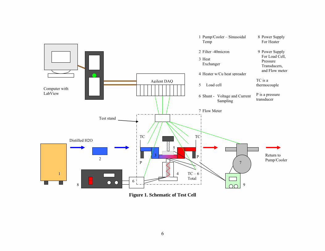
A test apparatus was designed to provide a way to determine the heat transfer through a SiC sample and supporting materials. (In the future, other materials and material stacks may be used.) These materials were cooled with a mini-channel heat exchanger that was designed and tested as a part of this project. Figure 1 is a block diagram that shows the experimental components of the test cell (test stand and required components). Figure 1 indicates that a cooling fluid flows from the cooler/pump and through a 40 micron filter before reaching the mini-channel heat exchanger (within the test stand enclosure). Distilled water was used to avoid contaminant materials that could damage the flow meter or interior passages of the chiller. The heat exchanger transfers thermal energy from a source (copper heater and stem) to the fluid. After flowing through the heat exchanger, the water passes through the flow meter. The flow meter contains a magnetic turbine and is calibrated to provide the mass flow rate (Appendix 3.3). The last components before the water returns to the cooler are the two flow valves. The valves are used in parallel for small flow adjustments. Each of the components and supporting instrumentation of Figure 1 are described in detail in following paragraphs. In addition, an image of the test components and supporting instrumentation (data acquisition (DAQ) and power supplies) are shown in Figure 2 on the supporting cart fabricated for transport of the apparatus.

6

Figure 1. Schematic of Test Cell

Return to Pump/Cooler

TC

P P

Distilled H2O TC

2 3

4

5

6

7

Filter -40micron 2

Heat Exchanger

3

Heater w/Cu heat spreader 4

Voltage and Current Sampling

Shunt - 6

TC – 6 Total

Flow Meter 7

5 Load cell

1

Agilent DAQ

Computer with LabView

Pump/Cooler – Sinusoidal Temp

1 Power Supply For Heater

8

9

8 9

Power Supply For Load Cell, Pressure Transducers, and Flow meter

TC is a thermocouple P is a pressure transducer

Test stand

7

Figure 2. Experimental Electronics Cooling Apparatus

3.1 Test Stand

The test stand was the primary group of experimental components for this project. „Test stand‟ refers to the mini-channel heat exchanger, the copper block (contains an electrical heater), and the aligning fixtures. Two test stand designs, the second was an evolution of the first, were completed for the testing. The first design (Figure 3) was smaller and involved fewer components than the second. The heat exchanger in the first design had channel lengths of ~11 mm. Unfortunately, this initial design had repeatability problems with the experiments and required re-design of the test stand. The heat exchanger was awkwardly bent which made flat alignment with the heating surface impossible. Also, the corner supports allowed the heat exchanger to slide.

Test Stand

Hyperion Mode DC - 18 VDC supply

Agilent 34970A

Sorenson DCR 600-1.5B Power Supply

LabView

8

Figure 3. The First Test Stand

The design of the second test stand had three goals set to insure a better outcome. First, the heat exchanger needed to be firmly held in place above the copper stem. The heater (electric) was contained within the copper heater block shown in Figure 3. At the top of the heater block, the material converges to a smaller square shape, the stem. The stem either by direct contact with the heat exchanger or through a material sample transfers heat to the fluid. Thus, good contact and positioning are important. The second goal was to have the heat exchanger alignment with the heater be adjustable. More specifically, the ability to adjust the position of stem contact under the heat exchanger was desired. The last goal was that the test stand needed to protect the heat exchanger from external convective air cooling and thermal conduction to the supporting cart.

Figure 4 shows an image of the second stand which will be described in the remainder of the experimental description. Figure 4 shows the copper heater, convection shield, the alignment structures, and a pressure transducer. The heat exchanger is located at the center of the test stand. Figure 4 shows a rigid alignment stand that was made for the second design. The second test stand provided better repeatability in the experimental measurements due to more rigid and better fabricated positioning parts. A detailed AutoCAD drawing is shown in Figure 5.

Fluid Inlet and Exit

Heat Exchanger Insulation/ Upper Plate

Test Stand Base

Heater

Load Cell

Heat Exchanger

9

Figure 4. The Second Test Stand

Copper Heater

Heat Exchanger

Alignment Stand

10

Figure 5. Section Drawing of the Test Stand

3.1.1 Copper Heater Block The copper heater block was designed to contain a cylindrical resistance heater (3/8 in diameter x 2 in length) and converge to a small (8 mm x 8 mm) square where the samples would be located. To promote a one-dimensional temperature distribution in the stem, high thermal conductivity copper was selected as the material. Figure 6 shows details of the copper block which holds the electrical heater (3/8 in diameter and ~2 in long). The stem which comes in contact with the heat exchanger is located at the top of the copper block.

Heater Alignment Stand

Alignment Components (Upper Plate, legs)

Heater alignment block (Phenolic)

Heat Exchanger & Glas-Therm block

Heater (copper)

Phenolic Block

Aluminum (heater wires to ext, heater mount)

Load Apparatus

Table

Macor Insulation (copper)

11

Figure 6. Sectioned Copper Heater Block

3.1.2 The Heat Exchanger Heat sinks and heat exchangers are commonly used for high temperature electronic applications. As operating conditions become more difficult, proper design will become more critical. Mini-channel heat exchangers (rectangular or round) have proven to be efficient at transferring large heat fluxes. The channels for the present mini-channel heat exchanger (635 m round channels in rectangular nickel substrate) were manufactured under the direction of Grady Yoder at Oak Ridge National Laboratory by electro-plating nickel on parallel fibers. The fibers were then removed by acid, resulting in channels that were slightly unparallel and out of center, but smooth. The expected surface roughness for this fabrication technique is 15nm (Papautsky et al., 1999).

Figure 7a shows an image of the mini-channel heat exchanger with the inlet/exit stainless-steel tubes. To simplify the fluid dynamics, it is desirable to have the tubing that connects with the heat exchanger to be in a straight line with the heat exchanger channels with few bends. However, the design also needs to accommodate secure mounting over the stem and provide good alignment. An image of the mini-channel heat exchanger is shown in Figure 7a. Figure 7b shows the three parts of the mini-channel heat exchanger: the mini-channel section (green), mixing chambers (blue, purple), and the inlet and exit tubes (yellow).

Stem

Copper Heater Block

Heater Bore

Mounting Flange - Base

12

(a)

(b)

Figure 7. An Image (a) and a Drawing (b) of the Mini-Channel Heat Exchanger

The heat exchanger, required to transfer 100 W/cm2, needed to transfer heat through a small area (8 mm x 8 mm). For the characterization of the flow and heat transfer within the channels, it was not necessary to use material samples for all tests. That is, the copper stem rather than a SiC sample was in contact with the heat exchanger for most of the testing. The contacting area of the stem and the heat exchanger were the same (8 mm x 8 mm) such that the heat exchanger mates with the stem. One of the methods to determine the heat input to the heat exchanger was measurement of the temperature increase of the cooling water. The heat exchanger width was chosen to closely match the stem size. The total heat exchanger width of 10.54 mm corresponds

13

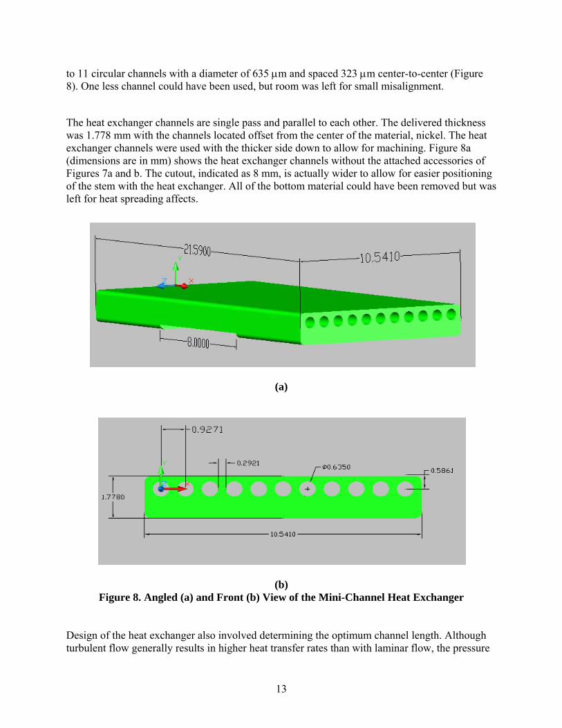
to 11 circular channels with a diameter of 635 m and spaced 323 m center-to-center (Figure 8). One less channel could have been used, but room was left for small misalignment.

The heat exchanger channels are single pass and parallel to each other. The delivered thickness was 1.778 mm with the channels located offset from the center of the material, nickel. The heat exchanger channels were used with the thicker side down to allow for machining. Figure 8a (dimensions are in mm) shows the heat exchanger channels without the attached accessories of Figures 7a and b. The cutout, indicated as 8 mm, is actually wider to allow for easier positioning of the stem with the heat exchanger. All of the bottom material could have been removed but was left for heat spreading affects.

(a)

(b)

Figure 8. Angled (a) and Front (b) View of the Mini-Channel Heat Exchanger

Design of the heat exchanger also involved determining the optimum channel length. Although turbulent flow generally results in higher heat transfer rates than with laminar flow, the pressure

14

loss with laminar flow in this channel is lower than that for turbulent flow. Thus, having laminar flow with developing hydrodynamic boundary and thermal layers along the length of the channels was a goal. If the channel length was too long and both the temperature and velocity profiles were fully developed, the cooling would not be optimal. In addition, the laminar flow may transition to turbulent flow. The channels were designed such that the heated section was located before fully developed hydrodynamic conditions for most Reynolds numbers (ReD) values considered. For the 635m diameter channels (as given by Eqn. 1), the fully developed hydrodynamic length is ~0.011m at a ReD of 350 (which corresponds to the lowest flow rate) and is 0.095m at a ReD of 3000. (Wilcox, 2000)

The actual heat exchanger channel lengths were 21.59 mm which locates the region of a fully developed velocity profile at the mid-point of the channels.

In fabricating the heat exchanger, a method of attaching the inlet and exit flow tubes (stainless-steel 625) to the channels had to be considered. In addition, the flow must be well-mixed after leaving the channels so that thermocouple measurements could reasonably represent the bulk water temperature increase. A mixing chamber design (Figure 9) was selected for attachment of the heat exchanger channels and the inlet/exit tubing. The mixing chambers (Inconel 600) were machined as two pieces which were later welded together to make one chamber. The purple half of the mixing chamber (Figure 9) has a rectangular slot where the heat exchanger was inserted and attached (Laser-welded - Precision Joining Technologies). The other half contains a hole for the inlet or exit fluid tube. There is an 8:1 ratio in cross-sectional area change between the mixing chambers and the 11 channels to minimize pressure loss and to provide even flow into the channels. The mixing chamber internal dimensions are 1.5 mm x 8.382 mm x 12.2 mm. The stainless-steel inlet/exit tubes (yellow) have an area ratio ~ 1:1 with the mixing chambers to minimize the pressure loss at the attachment region.

15

Figure 9. Two Halves of the Mixing Chamber and the Inlet (or Exit) of the Flow Tube

3.1.3 Alignment Stand The alignment stand holds the heat exchanger and the copper stem in specific positions relative to each other. The alignment stand must be able to allow the heat exchanger assembly to move small distances for installation and material expansion when heated. The stand also should have a way for applying a load to the top surface of the heat exchanger to ensure good contact between the heat exchanger and the stem. Figure 5 shows the assembled alignment stand (the upper plate, legs, and table). The mounting table contains the aligning holes (optical breadboard) used to locate the upper plate to the heater. The upper plate (Figure 10) was the alignment component for the heat exchanger; the heater and stem were aligned with an alignment block which squarely located them with the test stand legs. Provisions for the heat exchanger and the legs are indicated in Figure 10b.

16

(a)

(b)

Figure 10. Top (a) and Bottom (b) Views of the Upper Alignment Plate

The upper alignment plate fabricated from aluminum had notched locations (1 in x 1 in x 0.25 in) which mated with the supporting legs and a center section removed for the Glas-Therm/heat exchanger assembly (Figure 11a). Positioning the heated stem to have thermal contact with the heat exchanger was important for proper distribution of the applied heat flux. An alignment block (Figure 11b) made of phenolic plastic was used to locate the heater at the center of the test stand using the reference leg. The heater stand was made of a few materials (Macor, aluminum, and phenolic plastic) for insulating purposes, vertical adjustment, and stable positioning.

Leg Slots Heat Exchanger Position

17

3.1.4 Glas-Therm Block The heat exchanger required a block to position it in the upper alignment plate which would allow for vertical movement and minimize heat loss. A heat exchanger mounting block was fabricated from Glas-Therm which has thermal conductivity value of 0.6 W/mK and was easy to machine. The block was rectangular with a heat exchanger chamber cutout (Figures 11a and b). The heat exchanger was held in the block using a ceramic epoxy (Omegabond 1500 oF).

(a)

(b)

Figure 11. Glas-Therm Block with Respect to Tubing (a) and Upper Alignment Plate (b)

Glas-Therm

Heat Exchanger

18

3.1.5 Load Apparatus For enhanced experimental repeatability, a load apparatus was created to apply and record a force on the heat exchanger and copper stem. This force translates to a uniform contact pressure between the heat exchanger and the stem. The load cell is located at the top of the system (mounts on top of upper plate, Figures 5 and 12). Components of the load apparatus include the load screw, spring seats, plunger, spring, and aluminum block. The knob (Figure 12) (3/8 in fine thread) was used for making the pressure adjustment. The knob was threaded to the upper spring seat and applied a load through a spring (spring constant of 100 lbf/in) to the plunger. The system was fully seated (spring seat to spring seat) when the system was at steady conditions. This prevented overloading of the load cell during warm-up periods. The aluminum plate was for mounting the knob and securing the components to the upper plate. A stainless-steel tube held the aluminum plate and knob. The load was applied to the top surface of the Glas-Therm block. The load was transferred to the heat exchanger via the load cell and an aluminum plunger. The plunger had a 1¼ in diameter, approximately the same width as the Glas-Therm block.

Figure 12. Apparatus for Imposing Repeatable Thermal Load on the Copper Stem and

Heat Exchanger

Load Cell

Threaded Knob

Spring Seats

Aluminum Block

Plunger (applies load to Glas-Therm block)

Stand

19

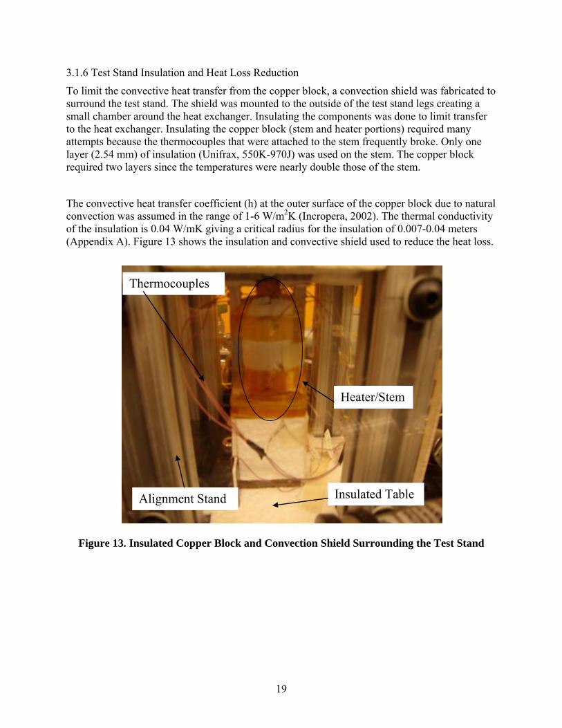
3.1.6 Test Stand Insulation and Heat Loss Reduction

To limit the convective heat transfer from the copper block, a convection shield was fabricated to surround the test stand. The shield was mounted to the outside of the test stand legs creating a small chamber around the heat exchanger. Insulating the components was done to limit transfer to the heat exchanger. Insulating the copper block (stem and heater portions) required many attempts because the thermocouples that were attached to the stem frequently broke. Only one layer (2.54 mm) of insulation (Unifrax, 550K-970J) was used on the stem. The copper block required two layers since the temperatures were nearly double those of the stem.

The convective heat transfer coefficient (h) at the outer surface of the copper block due to natural convection was assumed in the range of 1-6 W/m2K (Incropera, 2002). The thermal conductivity of the insulation is 0.04 W/mK giving a critical radius for the insulation of 0.007-0.04 meters (Appendix A). Figure 13 shows the insulation and convective shield used to reduce the heat loss.

Figure 13. Insulated Copper Block and Convection Shield Surrounding the Test Stand

Heater/Stem

Insulated Table Alignment Stand

Thermocouples

20

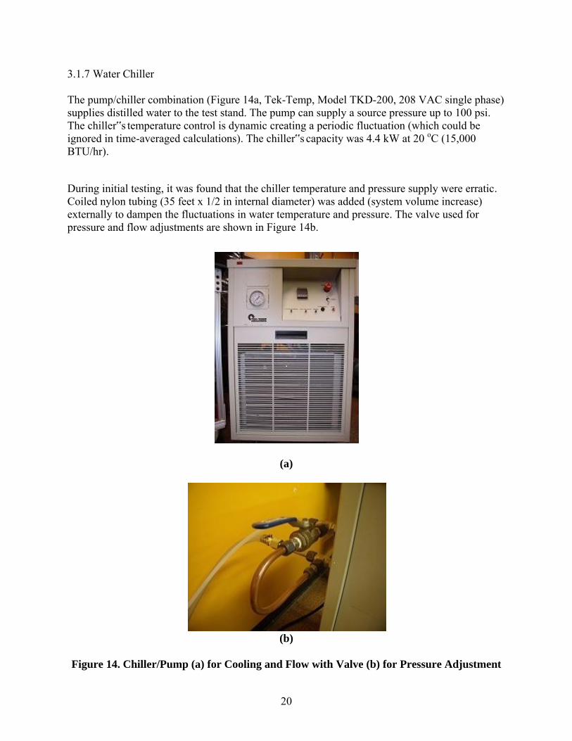
3.1.7 Water Chiller The pump/chiller combination (Figure 14a, Tek-Temp, Model TKD-200, 208 VAC single phase) supplies distilled water to the test stand. The pump can supply a source pressure up to 100 psi. The chiller‟s temperature control is dynamic creating a periodic fluctuation (which could be ignored in time-averaged calculations). The chiller‟s capacity was 4.4 kW at 20 oC (15,000 BTU/hr).

During initial testing, it was found that the chiller temperature and pressure supply were erratic. Coiled nylon tubing (35 feet x 1/2 in internal diameter) was added (system volume increase) externally to dampen the fluctuations in water temperature and pressure. The valve used for pressure and flow adjustments are shown in Figure 14b.

(a)

(b)

Figure 14. Chiller/Pump (a) for Cooling and Flow with Valve (b) for Pressure Adjustment

21

Other notable fluid components were a filter (Swagelok, SS-6TF-40) with a 40 micron filter located up stream of the system. To adjust the flow, two valves were located in parallel after the flow meter. One was a small adjustment valve (Nuclear Products Company) while the other (Nupro, SS-4D4S) offered large flow adjustment. The two valves (Figure 15) provided 22 g/s of flow at 50 psi (inlet pressure).

Figure 15. Two Valves for Gross and Fine Flow Adjustment

Flow Direction

22

3.2 Instrumentation

Characterization of the flow through the heat exchanger and the heat flux required measurement of the pressure difference across the heat exchanger, temperatures along the copper stem, temperatures at the inlet and exit of the heat exchanger, water mass flow rate, load-force values, heater voltage, shunt voltage, and heater current values. In addition to the above requirements, additional thermocouples were attached to the heater body and located in the chamber for an energy balance. A HP Agilent 34970A DAQ unit receives and relays the signals from the sensors. The Agilent unit is capable of monitoring four DAQ boards with 22 channels per board. For this experiment, only one board was used. LabView software (version 8.6.1) was used to record measured values. All runs were set to have a one second delay after each channel scan; data was recorded at three second intervals. Details of the LabView programs are given in Appendix F.

3.2.1 Thermocouples There were thermocouples located on the copper stem, copper block body, inlet and exit of the heat exchanger, and within the test stand convective heat transfer shield. The stem thermocouples were used for determining the heat flux transferred to the heat exchanger. The encapsulated T-type thermocouples (1/16 in diameter) located at the inlet and exit of the heat exchanger were used to measure the bulk temperatures to calculate the enthalpy rise of the water. The thermocouples were held in position using nylon compression fittings. A four-way fitting locates them in the fluid stream (Figure 16).

Figure 16. Inlet (or Exit) Flow Thermocouple with Pressure Port in the Bottom of the Four-

Way Fitting

23

The six T-type thermocouples which passed through insulation were attached to the copper stem (Omega, 0.005 in, butt welded) (Figure 17). The thermocouple beads were secured to the stem by epoxy (Omegabond, 1500 oF) in six 0.020 in diameter x 0.030 in depth holes (Figure 18). Various methods were tried for thermocouple attachment. Heating the copper block while curing the epoxy and vibration using a sonic bath to remove air pockets were both tried. The best method was to let the epoxy air dry but use more liquid bonding agent than suggested by the manufacturer. Thermocouple stress relief supports (aluminum) were added to help prevent breaking of the thermocouples while moving, calibrating, and testing (Figure 19).

Figure 17. Thermocouples (Circled) Attached to the Sides of the Stem

Heater

Stem

24

Figure 18. Location and Position References for the Stem Thermocouples

Figure 19. Stress Relief Clamps for Heater Thermocouples

TC Tension Relief

Thermocouples

25

3.2.2 Load Measurement The first load apparatus had a solid mechanical method for applying a load to the heat exchanger. This arrangement required continuous adjustment during warm-up. The apparatus was re-designed to incorporate a spring for warm-up and solid contact when steady conditions were reached. A threaded knob at the top of the apparatus applied a load through the upper and lower spring seats to the top center of the load cell. The load cell set on the plunger transmitted the load to the Glas-Therm block (Figure 12). The load cell (Omega, L8100-200-100) had a maximum load limit of 100 lbf and requires 10 volts DC excitation. Figure 20 is a drawing of the load cell and the loading apparatus. The load cell is shown in position between the lower spring seat and the plunger.

Figure 20. Load Apparatus and Load Cell on the Upper Alignment Plate

3.2.3 Pressure Transducers The pressure transducers (Omega, PX303-050A5V) had a 50 psi maximum limit and required excitation voltages in the range 9-30 VDC with output voltages in the range 0.5-5.5 VDC. Figure 21 shows an image of one pressure transducer for the exit flow. Calibration methods are described in Appendix C. The pressure transducer of Figure 21 was connected to the system

Load Cell Lower Spring Seat

Plunger

26

through a 4-way Tee at the exit side of the heat exchanger (flow taps). A second pressure transducer was located behind the test stand of Figure 21.

Figure 21. Pressure Transducer in Front of the Test Stand

3.2.4 Mass Flow Rate The mass flow rate of the water/cooling fluid was measured with a turbine flow meter. The flow meter provided a three-wire analog output to a signal transmitter (Omega, FLSC61) (Figure 22). The flow meter uses a magnetic wheel as a signal interrupter to produce a frequency signal. The signal was relayed to the transmitter where it was converted into a corresponding output voltage (milliVolts). Details of the mass flow meter calibration method are provided in Appendix C.

Test Stand Pressure Transducer

Flow Taps

27

Figure 22. Flow Meter with Transmitter

3.2.5 Electrical Supply Components The power supply for the pressure transducers, flow meter, and load cell was provided by one unit, a Hyperion Mode DC power supply (HY-WI-20-1.5) (Figure 24). The pressure transducers accepted a supply voltage in the 9-30 VDC range, the flow meter was in the range of 12-35 VDC, but the load cell was specific at 10 VDC. The power supply is set to 18 VDC. A voltage divider is used to drop the voltage to the required 10 volts for the load cells (Figure 23).

Figure 23. Schematic of the Voltage Divider Installed for the Load Cell Circuit

Flow Meter

Transmitter

Variable Resistor

28

Figure 24. Power Supply for Pressure Transducer, Flow Meter, and Load Cell

The heater power supply (Sorenson, DCR 600-1.5B) is 800 VDC and 2 A capable. Figure 25 shows the power supply, and Figure 26 shows the cylindrical heater. The heater (3/8 in diameter x 2 in length) could provide 200 W of power at 120 volts. The heater internal resistance was 76 Ohms and requires a housing ground. Early tests showed large power fluctuations over short time steps. To help with this issue, two capacitors (2500 F) were placed in line to smooth the power variation (Figure 27).

Figure 25. Power Supply for the Cylindrical Heater within the Copper Heater Block

29

Figure 26. Cylindrical Heater Located within the Copper Block (on the Right)

Figure 27. Schematic of the Capacitors Connected to the Heater

Heater Power Supply Capacitors

30

4.0 EXPERIMENTAL PROCEDURE

The procedure to run an experiment included adjusting the chiller temperature and pressure, flow rate, contact load, and heater and sensor power. Prior to performing a test, the electrical equipment and the cooling/pump were run 20-30 minutes prior to data collection to allow for the temperature of the involved circuits to stabilize.

4.1 Water Chiller

The inlet fluid temperature, 20 oC, was set at the chiller/pump unit using the available PID (Proportional Integral Derivative) controller. The fluid temperature measured at the inlet to the heat exchanger varied by a few degrees, depending on the flow rate of the system. The inlet/exit heat exchanger thermocouples (TC 13 & 14 – channels 113 and 114) and the number 1 stem thermocouple (TC 1 – channel 101) were monitored for steady periodic conditions. The steady periodic conditions were selected by viewing the temperature fluctuations over a range of time (on the order of an hour, Figures 28 and 29). The steady periodic peak-to-peak variation ranges from 0.5oC at low flow (highest T in fluid) to below 0.1 oC at higher flow rates. The effect that the fluctuations have on the calculations and analysis is minimal for long periods. Figure 30 shows that the temperature fluctuation between the inlet and exit of the heat exchanger is small (0.04 oC standard deviation). Also, the variation of the inlet fluid temperature would have a small effect on the stem calculations for energy flux with temperatures of 100oC at TC1 and 70oC at TC3 (Figure 31).

Figure 28. Sample Temperature Plot for Inlet Fluid Thermocouple

23

23.2

23.4

23.6

23.8

24

24.2

24.4

24.6

24.8

25

0 500 1000 1500 2000 2500 3000 3500 4000

Tem

pe

ratu

re (

oC

)

Time (Seconds)

31

Figure 29. Sample Stem Temperature Trend (Thermocouple #1, Same Test as in Figure 28)

Figure 30. Temperature Difference between Inlet and Exit of Heat Exchanger

98

98.2

98.4

98.6

98.8

99

99.2

99.4

99.6

99.8

100

0 1000 2000 3000 4000

Tem

pe

ratu

re o

C

Time (Seconds)

2.4

2.45

2.5

2.55

2.6

0 500 1000 1500 2000 2500 3000 3500 4000

Tem

pe

ratu

re o

C

Time (Seconds)

32

4.2 Pressure and Flow Rate

The inlet pressure in the coolant lines was set to approximately 50 psi (52 psi max) at the chiller/pump. The pressure setting was adjusted by the ball valve located at the rear of the unit. This ball valve is a bypass valve which diverts unneeded output flow back to the cooler/pump. With the system set at 50 psi, a maximum flow rate of 22 g/s was possible.

The heat exchanger flow rates were in the range of 2-22g/s. The desired flow rates were obtained by adjusting the low flow and high flow needle valves located downstream of the flow meter and simultaneously adjusting the line pressure (Figure 15). A large needle valve is used for gross adjustment and a micro valve is used for fine adjustments. Mass flow rates below 3-3.5 g/s resulted in high flow fluctuations and were difficult to quantify.

4.3 Contact Load

The contact load (pressure) at the interface of the heat exchanger and the stem was relatively low (20 lbf ~ 200 psi). repeatable conditions were important for testing. This load is suspected to be part of the repeatability problem. It was later found that the load was insufficient to overcome the friction between the load plunger and the upper plate (Figure 12). As will be described later, the repeatability problems were resolved.

4.4 Power Supplies

The electrical power applied to the heater within the copper block was set to the desired rating by adjusting the current dials, course and fine, on the power supply. The heater resistance was 76 Ohms at room temperature and increases slightly as the heater warms. The voltage, current, and power are monitored using LabView DAQ software. A shunt, installed in series with the heater supply power, provides a voltage drop that translates to a current value. The shunt (0.02 Ohm) has an accuracy of 0.31% as reported by the manufacturer (RC Electronics). The voltage drop is measured by the Agilent DAQ unit. The imposed power on the heater drifts with time. Thus, monitoring and adjustment is needed periodically during runs. The only requirement by the power supply for the load cell, pressure transducers, and flow meter (Figure 24) was to verify that it was set at 18 VDC to prevent over-powering the load cell.

33

5.0 RESULTS AND DISCUSSION

A test stand was designed to provide two methods for energy balance verification. The copper stem, equipped with thermocouples at fixed distances along two sides, provided temperature values used to determine the heat flux passed to the heat exchanger. The heat flux determination was primarily a conduction problem and is considered in Section 5.1. Analysis of the convective heat transfer providing the enthalpy rise in the water within the heat exchanger was not as straight forward as the conduction heat transfer analysis (Section 5.2). The convective heat transfer within the heat exchanger was described in terms of Nusselt numbers and comparisons are made with established correlations. The analysis of the heat transfer includes conduction along the nickel heat exchanger material.

5.1 Conduction Heat Transfer through Copper Stem

Two calculations associated with the heat exchanger analysis were the conductive heat flux through the stem and the enthalpy rise in the working fluid. For a given set of conditions, comparisons of the enthalpy rise and conductive flux provide confirmation of the heat transfer. This section was primarily concerned with the quantification of heat conduction through the stem. The evaluation of the heat conduction through the stem was performed using the voltages (and thus the temperatures) provided by six thermocouples placed on opposite surfaces of the stem (Figure 31). The opposing surfaces correspond to the inlet and exit of the mini-channel heat exchanger.

Figure 31. Six Thermocouple Positions on Copper Stem (Upper Portion of Heater Block)

The thermocouple data averaged over a few hundred seconds, after reaching a steady-state condition for each water flow rate and heater power input setting, were analyzed and compared. Figure 32 is a plot of the temperatures obtained from the thermocouples located at the relative position number on the stem (Figure 31) for a water mass flow rate of 7g/s and a 90 W heater

1

3 2

6 5 4

Heater

Stem

X

Y

Heat Flux

34

input. The #1 and #4 thermocouples are both shown as position 1 in the plot because they are at the same level on stem (same distance from the tip). The same method is used for thermocouples 2-5 and 3-6.

Figure 32. Temperature Distribution along Copper Stem for Water Flow Rate of 7g/s

Initially, it was thought that the nonlinearity of the profiles of Figure 32 were due to uncertainty in positioning or temperature. However, this is not believed to be the case, after some investigation, as explained in the next several paragraphs. First, the influence of thermal expansion on the final location the thermocouples were determined (i.e., differences between the two temperature profiles). The chemical composition of the stem is 99.9% oxygen free copper. Thus, expansion and movement of a thermocouple may be possible (Chemical analysis in Appendix G). Copper has a thermal expansion coefficient ( ) of 9.4 x 10-6 in/oF. The stem is approximately 8 mm square and has a length of 0.01194 m (L). The linear expansion due to an increase in temperature is given by (Holman, 2001):

For a temperature difference of 200oC (which is the greatest temperature rise expected), the thermal expansion is 2.387 x 10-5 m. This value has a negligible influence on the thermocouple location and, thus, on the measured axial temperature profile.

Another reason for a nonlinear profile may be the heat loss from the vertical surfaces of the stem. The stem contains one layer of insulation with a k value (conduction heat transfer coefficient) of

75

80

85

90

95

100

105

110

115

120

0 1 2 3 4

Tem

pera

ture

(o

C)

Postion #

TC's 1-3

TC's 4-6

35

0.04 W/m K. The maximum heat transfer coefficient value of 6 W/m2 oC on the inside of the chamber was estimated by treating the stem surfaces as flat plates in the presence of natural convection. The heat flux from the stem sides is at most 330 W/m2. The total transfer is (stem surface area = 4.064 x 10-3 m2) 0.134 W. Thus, the nonlinearity in the stem temperature profile is not due to heat loss from the stem.

Since neither the heat loss from the stem vertical surfaces nor the thermal expansion is responsible for the measured non-linear temperature profile, another analysis was performed to consider the effect of thermocouple placement on the stem temperature profile. There could be significant error due to machining or thermocouple bead placement. Machining error often is a directional error, that is, if a hole is offset in one direction due to machining error, typically all other errors will be offset in same direction.

Measurement of the thermocouple hole positions was performed after machining. An average value for x (0.0047 m) is used for the following analysis. The location of the thermocouples within the 0.020 in diameter holes in the copper stem also has an uncertainty. The bead diameters of the thermocouples (2 - 0.005 in thermocouple wires) are 0.01-0.011 in This translates to a + 0.005 in vertical position uncertainty for each thermocouple in the stem.

Figure 33 shows the temperature profile along the stem with ±0.005 in. thermocouple placement indicated by horizontal error bars. For reference, the dashed line indicates a linear temperature profile. The uncertainty of the temperature difference, thermocouple to thermocouple, is less than 0.5 oC. The uncertainty is the standard deviation of the temperature difference for the fluid thermocouples during calibration (no statistical analysis). Figure 33 reveals that positioning uncertainty for the thermocouples would not correct the temperature profile along the copper.

36

Figure 33. Stem Temperature Profile ( ±0.005 in Thermocouple Placement)

The temperature profile in the stem is better understood by considering a temperature contour plot involving the heat exchanger obtained, in part, by CFD calculations. Figure 34 shows a sketch of the expected stem temperature profile due to contact with the heat exchanger. The temperature distribution within the heat exchanger (Figure 35) was calculated by Fluent, a commercial CFD code. The stem temperature contours were visually extrapolated from the heat exchanger temperature contours.

Figure 34. Sketch of Expected Heat Conduction Flux Directions within the Stem

75

80

85

90

95

100

105

110

115

120

0.000 0.005 0.010

Tem

pera

ture

(o

C)

Position from TC1 or TC4 (m)

TC's 1-3

TC's 4-6

Fluid

Heat Exchanger

Stem Thermocouples

37

This contour plot suggests that the heat flux calculation on the stem is not one-dimensional near the heat exchanger. The high heat transfer rate at the upstream contact point of the heat exchanger and the stem has the effect of causing a higher conduction heat transfer rate at that corner of the stem. Thus, the four thermocouples furthest from the heat exchanger (1, 2, 4, 5 – Figure 31) should be used to determine the heat flux through the stem. The conduction rate using the thermocouples is 72.48 W (average of both sides). The enthalpy change for the same condition (7 g/s flow) is 72.66 W. These values show that there is very good agreement between the energy conducted through the stem and the change in enthalpy of the cooling fluid. The energy balance for the stem and fluid (2-22 g/s) is plotted in Figure 35. The solid line indicates a 1:1 balance. The heat flux passing through the 0.64 cm2 (8 x 8 mm) stem at the 7 g/s conditions is 113 W/cm2. This meets the requirement of 100 W/cm2. In pre-testing, ~160 W/cm2 heat transfer was observed an interface temperature (stem-heat exchanger) of 90 oC at 7 g/s flow in the heat exchanger. The low temperatures at the interface indicates that the thermal resistance between the stem and heat exchanger could be doubled, from the insertion of SiC device, before the temperature limit would be reached.

Figure 35. Energy Balance: Stem Conduction and Enthalpy Rise of Water

38

5.2 Convective Heat Transfer within Mini-Channel Heat Exchanger

5.2.1 Numerical Analysis The convective heat transfer coefficient within the heat exchanger is given by (Incropera, 2002)

where q" is the heat flux (Q/A), and Ts is the local channel surface temperature. The area for convective heat transfer within a heat exchanger channel is

The area is a product of the channel diameter (D) and the heated length (L) of the channel. The average bulk temperature, Tm, is

The total heat transferred to the channels, Q, is defined as (Incropera, 2002)

In Equation 6, Cp is the constant pressure specific heat, is the mass flow rate, and T is the difference between the bulk inlet and outlet temperatures.

Figure 36 shows the calculated enthalpy change in the heat exchanger fluid, Q, recorded over three consecutive days of testing. There are discontinuities in the curve at 7 and 11 g/s. The discontinuities are believed to be due to repeatability issues connected with the contact resistance. At the writing of this report, not all of the experiments had been repeated multiple times. However a measure of confidence in the values comes from two months of setup and validation tests. Before final testing began (for the results presented here), validation tests were run to help with test stand adjustments. These tests were all performed at 7 g/s. The heat transfer values and temperature conditions found in the first group of data (before the first discontinuity) are very close to the conditions recorded in the pre-tests. Moreover, the maximum difference in the heat transfer rates at the discontinuities of 11 g/s is below 2%. At flow rates of 20 g/s and greater, the heat transfer rate to the heat exchanger would normally be expected to increase when the ReD are in the range of laminar to turbulent flow transition. However, there is a decrease in heat transfer. This decrease in the heat transfer rate near 20 g/s is believed to be a result of the plunger (last component in load apparatus transferring force to the heat exchanger) sticking. The repeatability issues and potential plunger sticking problems would need to be further explored if more work was undertaken.

39

Figure 36. Heat Transfer Rate to the Eleven Channels of the Heat Exchanger

The surface temperature for each channel within the heat exchanger is unknown, so an estimate is used. Using the thermocouple values in the copper stem and the thermal properties for the copper and nickel (heat exchanger), a temperature was estimated at the bottom of the channels. This value was averaged with the bulk temperature to estimate the surface temperature for the channels and assumed the same temperature around each channel. Figure 37 shows a two-dimensional color contour plot for a plane along a channel axis that was obtained from a three-dimensional CFD simulation (Fluent code). This simulation assists in the explanation of the convective heat transfer coefficient calculation and is useful for comparison of the results with existing heat transfer correlations. The plane for the color contour plot shown is located at the mid-point of the heated section. Figure 37 shows that the surface temperature varies relatively little from 31.4 oC to 32.2 oC with an average of 31.8 ± 0.4 oC.

70

71

72

73

74

75

76

0 5 10 15 20 25

Heat

Tra

nsfe

r to

Heat

Exch

an

ger

(Watt

s)

Flow Rate (g/s)

40

Figure 37. Calculated Temperatures (K) inside and outside the Center Channel (ReD of

1260)

The value for L (heat transfer length of the channels in Eqn. 4) is important for accurate results. As seen in Figure 34 the heat exchanger extends beyond the stem and acts to spread the heat by conduction. The heat transfer length selected to represent the region of convective heat transfer could be the channel length (gives a low NuD value), stem-to-heat exchanger contact length, or more appropriately the actual length along the channel in which the heat is conducted in the solid wall (i.e., conjugate heat transfer effects obtained by CFD simulation).

Figure 38 is a plot of NuD with ReD for two of the above situations – shortest and longest heat transfer lengths (8 mm and 21.59 mm). NuD is defined as (Incropera, 2002)

In Eqn. 7, D is the diameter of a channel, and k is the thermal conductivity of the water. The convective heat transfer coefficient, h, is determined from Eqn. 3. The Reynolds number was based on average velocity at the inlet temperature (which varies relatively little from the bulk temperature) and is defined as

where is the fluid density , the diameter of the channels, V is the average velocity, and is the dynamic viscosity of water.

41

Figure 38. NuD Resulting from Use of the Shortest and Longest Heat Transfer Lengths

Figure 38 shows that a NuD profile for ReD in the range 0-1900 is followed by a step change in the profile for larger ReD (a step at 1100 Re exists but is much smaller). The raw data for the three segments of a NuD curve were obtained on consecutive days. The sudden change in a NuD curve is due to repeatability issues which vary with daily setup. The decrease in all of the NuD curves near ReD of 3800 is believed to be due to load plunger issues. These repeatability issues were described earlier in connection with Figure 36 correspond to a decrease of approximately 13% and are not considered fatal to interpretation of the experimental results.

CFD simulations were used to determine more appropriate values for the heat transfer length. A two-dimensional model was used to represent the maximum thermal spreading, and a three-dimensional model was used for a mid-range flow rate (7 g/s). The minimum heat transfer length is the length that the stem makes contact with the heat exchanger (8 mm). Figure 39 shows the contact interface of the stem and the heat exchanger. The stem is slightly recessed into the heat exchanger. The heat exchanger and stem together form a line of contact parallel to the fluid flow. This line of contact is 8mm in length.

0

5

10

15

20

25

30

0 1000 2000 3000 4000 5000

Nu

D

(hD

/k)

ReD

Nu - 8mm length

Nu - Length 21.59mm

42

Figure 39. The Heat Exchanger and Stem Form a Line of Contact Parallel to Fluid Flow

Figure 40 shows a contour plot of the channel region calculated by the commercially available CFD code, CFDACE. For a flow rate of 2 g/s and a heat flux of 70 W/cm2, the two-dimensional numerical simulation shows how the channel wall thickness allows the imposed heat flux to diffuse such that the heated length is not the same as the contact length between the stem and heat exchanger. The estimated length from the CFD simulation is ~14.5 mm and will vary with the heat transfer and mass flow rate in a channel. To determine the heated characteristic length from the temperature contour plot, an examination of the thermal boundary layer is required.

Figure 40. Temperature Contour Plot for a Two-Dimensional CFD Solution (ReD of 1260)

Estimated Longest Heat Transfer Length ~ 14.5mm

Channel Length 21.59mm

Fluid Channel

Heat Exchanger

Heater

Stem Contact Length

Flow Direction in Channels

43

The thermal boundary layer is considered here to be the region where there are significant differences (more than 3 oC) between the fluid and channel surface temperatures. The length of the thermal boundary layer was taken as L. A three-dimensional simulation was also performed. For the three-dimensional length estimate, axial and radial temperatures were taken into account. For a ReD of 1260 (mass flow rate of 7 g/s), the measured bulk temperature increase of the fluid from the inlet to exit of the heat exchanger was 2.46oC. The three-dimensional model gave a temperature increase of 2.5oC for the same conditions which is in very good agreement with the measurements. Unfortunately, the three-dimensional model required a large numbers of cells and extended run times were required. For this reason, the three-dimensional simulations were performed only at 7 g/s (1260 ReD). The analysis for the heated length for this model provides a length of approximately 11mm. Figure 41 shows the temperature contour plot for the conditions tested.

Figure 41. Two-Dimensional Temperature Contours (from Three-Dimensional Model)

along the Channel Centerline (ReD of 1260)

Not having multiple contour plots meant that the temperature profiles for all the experimental flow rates would not be available. To fill the gap for all other flow rates tested, an exponential profile is assumed to fit the lengths as a function of flow rate for simplicity. The exponential curve was fit to three values: (the shortest expected length) 8mm (22g/s), 11mm (7g/s from a three-dimensional CFD model), and14.5mm (2g/s, the lowest flow rate from a two-dimensional CFD model). The values for the heated lengths were then estimated for each of the flow rates.

Figure 42 is a plot of NuD with ReD which is determined from the average velocity for water in the channels and the mean bulk temperatures. The NuD number is determined with an area based

Estimated Heat Transfer Length ~ 11mm for 7 g/s

8mm contact point – stem to HX

Fluid Channel

44

on a variable heat transfer length (curve fit). The NuD with variable heat transfer length is compared to NuD for constant lengths corresponding to the channel length and the contacting interface length (between the heat exchanger and copper stem). The plot indicates that heat diffusion in the walls of channels and tubes may strongly affect NuD and may need to be taken into account. For the situation of a constant heat flux with fully developed laminar flow, NuD is 4.36. We do not have fully developed flow and, thus, NuD should be above 4.36 as in Figure 42.

Figure 42. Comparison of Three Characteristic Heat Transfer Lengths

Comparisons with established heat transfer and flow correlations assist in validation of the assumptions made with respect to the heat transfer length described in preceding paragraphs. Heat transfer correlations are available for various entry conditions: combined thermal and hydrodynamic, only hydrodynamic, or only thermal. Each of the conditions is available with either uniform heat flux or constant temperature at the channel wall. Selected correlations are now considered. The hydrodynamic boundary length is calculated as (Wilcox, 2000)

The x value (fully developed length) is 11.3 mm at the lowest laminar mass flow rate to 114 mm at the highest (358 < ReD < 3600). For turbulent flow (3600 < ReD <3900), the length of the entry region is described by (Wilcox, 2000)

0

5

10

15

20

25

30

0 1000 2000 3000 4000 5000

Nu

D

ReD

Nu - 8mm length

Nu - Length 21.59mm

Nu - variable length

45

The length (x) associated with a diameter of 0.000635 m is 0.00635 m or roughly 1/3 of the channel length. It is important to know where the temperature profile will become fully developed. An estimate of the thermal entry length is given by (Wilcox, 2000)

In Eqn. 11, the Prandtl number (6.996) is evaluated at the mean bulk temperature. The estimated entry lengths are 0.0795 to 0.866 m.

5.2.2 Comparison with Experimental Data The first comparison between the experimental data and a heat transfer correlation is for flow with developing thermal and hydrodynamic profiles (Figure 43). A correlation for the mean Nusselt number (Shah (1978)) used for small channels with a combined entry length and uniform heat flux is (Young, 2008)

To illustrate the consequences of the selection of L, L in Figure 43 is chosen as the entire channel length (21.59 mm) for simplicity rather than the heat transfer length derived from CFD simulations. Thus, the entire channel length is selected for both the evaluation of Eqn. 12 and the experimentally determined NuD. Here, Ref is the Reynolds number based on an average fluid velocity, and the Prandtl number is obtained using the mean bulk temperature. The bulk viscosity (from the mean bulk temperature) and the estimated viscosity at the wall are f and w, respectively. With this choice of heat transfer length, Eqn. 12 appears to overestimate NuD values relative to those determined experimentally. We know from the CFD simulations that the entire channel length is not the optimum choice for L. Thus without the CFD simulation, it is not clear a priori what value of L should be used in the experimental data reduction or for use with heat transfer correlations.

46

Figure 43. NuD (Shah (1978)) Correlation for Combined Thermal and Hydrodynamic

Entrance Length with NuD Determined from Experimental Measurements (L = 21.59 mm)

Comparison of NuD that are experimentally obtained here with those from heat transfer correlations available in the literature can provide additional confirmation of the measurement methodology. That is, provided L from the CFD calculations (or a more judicious choice than simply guessing) is chosen for use in reduction of the measured data when its value is otherwise unclear. Most available heat transfer correlations for the flow and thermal entry region within a circular tube were derived for either a uniform heat flux or isothermal wall boundary along the entire tube. This is not the case for the present experiments as the tube is heated only over a section of the tube and only over a portion in the circumferential direction. In addition with regard to the entry region, heat transfer correlations are available for developing temperature profiles assuming a fully developed velocity profile and for velocity and temperature profiles which simultaneously develop from the inlet. In this work, the heated tube section is downstream from the inlet, and Pr is ~7. Thus, the thermal and velocity profiles do not develop at the same rate, and the starting location of the thermal boundary layer does not coincide with that of the velocity boundary layer. Although the requirements of the available heat transfer correlations do not quite match the actual experiments, it is expected that they will still bracket the experimental NuD values.

For conditions of a uniform heat flux and for thermal and velocity profiles which develop from the inlet, a local NuD-x correlation (local axial location denoted by the subscript –x) is given by Churchill and Ozoe (Bejan, 1995) (Churchill, 1973):

0

2

4

6

8

10

12

14

16

18

20

0 1000 2000 3000 4000 5000

Nu

D

ReD

Nu - Length 21.59mm

Shah combined entry

47

Here, the Graetz number (Gz) is defined as

and the Prandtl number for the mean bulk fluid temperature (Pr) is 6.996. x* is defined as

Equation 13 was numerically integrated from the channel entrance to the end of heated copper contact region (from x = 0 mm to x = 14.795 mm) to obtain average values of the Nusselt number (i.e.,

) for a range of ReD. Although not entirely physically

correct, it is reasonable to choose L = 14.795 mm for use with Eqn. 13 for simplicity. For purposes of comparison, the NuD values obtained from the integration of Eqn. 13 are plotted together with the experimental NuD values (which also use L determined from CFD simulations and referred to as a variable heat transfer length in the legend) in Figure 44. The two curves compare reasonably well considering the typical uncertainty in a heat transfer correlation is + 25%.

48

Figure 44. NuD Derived from the Churchill and Ozoe Correlation (1973) Plotted with

Measured Values

For a thermal entry region alone, assuming a fully developed velocity profile (Hagen-Poiseuille flow), a correlation for NuD-x for uniform heat flux is (Bejan, 1995; Shah and London, 1978),

Eqn. 16 is essentially a fit of the classic Graetz solution (Kakac et al., 1987). Eqn. 16 was numerically integrated along the heated copper contact length (from x = 6.795 mm to x = 14.795 mm with the inlet as the origin) to yield NuD for a range of ReD. The integration range used for this correlation is different from that used for Eqn. 12 because of the assumptions of fully developed flow (which does not actually exist) and a developing thermal profile (along this length). This choice of the integration limits emphasizes the effect of the developing thermal

5

10

15

20

25

30

35

0 1000 2000 3000 4000 5000

Integration of Eq 13 from 0 mm-14.795 mm

variable heated lengthN

uD

ReD

49

profile. (In Eqn. 16, Pr and ReD are evaluated at the mean bulk temperature.) The NuD values obtained from the integration of Eqn. 16 and the experiments are plotted together in Figure 45. Figure 45 shows that the integration of this correlation over the selected integration limits underestimates NuD obtained from the experiments (which use L from the CFD simulations) over this ReD range.

Figure 45. Comparison of Shah and London (1978) Uniform Heat Flux Correlation with

Experimental Data

A heat transfer correlation (Kakac et al., 1987) for the mean Nusselt number, NuD, that was originally derived for flat ducts has also been used for circular ducts (Bejan, 1995) is given by

This correlation is for simultaneously developing temperature and velocity profiles within a tube with isothermal wall conditions, and x* and Pr are defined in the same way as in Eqn. 16. Eqn. 17 was evaluated at x =14.795 mm (the end of the heated copper contact region) to provide NuD

5

10

15

20

25

0 1000 2000 3000 4000 5000

Integration of Eq 16 from 6.795 mm-14.795 mmvariable heated length

Nu

D

ReD

50

for comparison with those obtained from experiments for different ReD in Figure 46. The correlation for isothermal walls (Eqn. 17) agrees well with NuD derived from the present measurements.

Figure 46. Comparison of Experimental Data with a Correlation for Entry Flow with

Constant Surface Temperature (Kakac et al., 1987)

To summarize, Figure 47 shows Eqns. 12 to 17 together with the experimentally acquired NuD. Eqns. 12 and 17 are the best fits to the experimentally determined NuD (variable heat transfer length). However, all the correlations compare reasonably well with the experimental values. This agreement among NuD obtained by different methods provides a measure of confidence in the results. (It is mentioned in passing that for ReD values above 700 to those in the turbulent range, the fully developed hydrodynamic region is beyond the channel length.) The measured heat transfer values involved physical/mechanical errors which resulted in values 7-11% lower than expected. The contact resistance for the thermal grease was nearly 5 times higher than the

51

manufacturer specified, indicating poor contact. This is known because losses in the stem are negligible. The uncertainty in NuD is addressed in Appendix B. However, statistical aspects of the uncertainty are not fully accounted for due to limited testing repetitions (Note: the first part of the experimental data is used for all comparisons.)

Figure 47. Comparison of All Correlations with Experimentally Determined NuD

52

6.0 FLOW CHARACTERIZATION

6.1 Head Loss

The pressure drop across the heat exchanger was measured for all flow passages between the inlet and exit pressure sensors of Figure 1. It is important to understand the influence of each flow element on the available pressure. The heat exchanger channels themselves are of interest for fluid flow characterization but are located between the inlet and exit pressure transducers with other attachments or accessories. The measurement of pressure drop (P) across a channel section can be used to evaluate the flow losses. This means that the P measurements obtained here will necessarily be greater than those of the heat exchanger channels alone. To compare the experimentally determined friction factors of the heat exchanger tubes with existing friction factor correlations, for example, the flow effects due to the heat exchanger accessories need to be removed. Figure 48 shows a sectioned view of the heat exchanger (with connecting flow passages) used in the experiments. Pressure taps are located at either end of the (yellow) tubes, and the letters correspond to the positions listed in Table 1.

Figure 48. Sectional View of Heat Exchanger Showing the Flow Path

Subtraction of the pressure drops resulting from components other than the channels is now considered. To account for all pressure losses in the system Eqn. 18 is used (Maynes, 2002).

Here, is the densityV is the velocity, f is the friction factor for a channel (a function of tube surface roughness and diameter), L is the component length, D is the characteristic diameter, and KL is the pressure loss coefficient which accounts for losses due to bends and expansions, for example.

A

B

C

D

F

E

53

The pressure loss coefficient is defined as KL= PL/(V2/2) where P is unknown for each section. KL is an empirical constant, and tabulated values for different flow configurations are available (Idelchik, 1986). Figure 49 shows where component pressure drops occur (Table 1). The following paragraphs describe the path through the channels with short descriptions on how each flow situation (change in flow direction, expansion, contraction, etc.). At the ends of the two tubes (yellow) of Figure 48, there are tees with ports (not shown) that are connected to pressure transducers by tubing. Starting at the left side of Figure 48, the flow moves through the ¼” tubing to the mixing chamber. The pressure drop in this short tube is neglected. At this point, the flow enters the inlet of the mixing chamber (two pieces welded – blue/purple). The area of the inlet tube is 2.44 mm2 while the area of the mixing chamber using the hydraulic diameter (Dh) is 4.4 mm2. The hydraulic diameter is (Idelchik, 1986)

The hydraulic diameter, the equivalent diameter for a rectangular channel, is a function of the width, a, and the diameter, b. This is the first event – an expansion due to a change in flow area. After the flow enters a chamber, it must change direction (B of Figure 48). This event (change in direction) can be represented as an elbow. The elbow flow occurs again at the entrance to the channels. Instead of two separate events, the flow through the mixing chamber is treated as a double elbow, one event. For simplicity, the bend radius for the flow is estimated at ½ the chamber width. This changes the hydraulic diameter for the flow. The new hydraulic diameter is 2.54 mm2.

The entrance to the heat exchanger channels is the next event. This location has two flow effects to consider. First, there is a contraction from the mixing chamber to the heat exchanger channels. In addition, the channels have a sharp entrance. The same analysis is used for the exit side of the system where there is an expansion from the channels to the mixing chamber, another double elbow, and two events again at the exit of the mixing chamber to the ¼ tubing.

Table 1 summarizes the flow events and their contribution to the total P. The equations in the table are used to estimate KL values. With the KL coefficients, the head loss is calculated by dividing Equation 18 by ρ. The head loss for each flow event is plotted with ReD within the channels in Figure 49 using the average velocity which was calculated using transport properties determined at 20 oC. Figure 49 shows that the head losses are greatest for the entrance and exit regions of the channels.

54

Figure 49. Head Loss Values (Idelchik, 1986) Plotted with ReD for Each Flow Situation

0

2

4

6

8

10

12

14

16

0 2000 4000 6000

He

ad L

oss

(m

2/s

2)

Reynolds Number

Head Loss Inlet Channels

Head Loss Exit Channel to Mixing Chamber

Head Loss Inlet to Chamber

Head Loss Exit Chamber to Tube

Head Loss 2 Double Elbows

55

Table 1. Equations (Idelchik, 1986) Used to Calculate Loss Coefficients for a Particular Flow Event Neglecting fr (Minor Loss

Coefficient)

56

6.2 Characterization of the Channels – Pressure Loss

Mini- and micro- channels provide enhanced heat removal but at the expense of increased P (pressure difference) so proper optimization must be considered. Obtaining accurate pressure differences by experiment or numerical simulation is therefore critical for thermal designs if pumping energy savings are desired. As described previously, the inlet and exit pressure measurements were taken across the entire heat exchanger assembly, which includes tube inlets/exits, mixing chambers, and heat exchanger channels. The pressure losses due to the connecting components were estimated and subtracted from the P measured from the test stand. A corrected P for the heat exchanger channels was then obtained and used in the following analysis. Although there are uncertainties in this indirect method (Appendix 2.6), it is a well-known engineering technique and reasonable results can be obtained. Correlations for estimating the departure from Hagen-Poiseuille flow (White, 1974) and the turbulent transition flow as a function of Reynolds number were used to help validate the calculated friction factor. In the current work, the channel flow behavior is described by the friction factor, f. The pressure drop across the channels can be used to determine f (Wilcox, 2000):

In Eqn. 20, V is the local average velocity. All Reynolds numbers (ReD) are based on the average velocity and mean bulk temperature of the water. Figure 50 shows the measured pressure drop across the heat exchanger, the measured pressure drop minus the pressure drop from head loss calculations, and the pressure drop given by the Poiseuille equation.

57

0

10000

20000

30000

40000

50000

60000

70000

Poiseuille

With Head Loss Without Head Loss

0 500 1000 1500 2000 2500 3000 3500 4000

Pre

ss

ure

Dro

p (

Pa)

ReD

Figure 50. Measured P across the Heat Exchanger, Measured P Minus the P from

Head Loss Calculations, and the P Given by the Poiseuille Equation

Evaluating the channel friction factor (f) for this case has a degree of uncertainty because a measurement of the surface roughness for the channels was unavailable. The channels were manufactured at Oak Ridge National Laboratory using an electroplating method in which nickel was accumulated on fiber wires. The fibers are chemically dissolved after the process is finished. Figures 51a and b are scanning electron microscope (SEM) images of the heat exchanger channels. The images show that the channels (635 m diameter) have smooth circular edges. The range of surface roughness () for these channels is approximated as 15nm to 1.5 m (a smooth drawn tube) (Papautsky, 1999). The /D (ratio of surface roughness to tube diameter) is a maximum of 0.0024 mm/mm. Using a Moody diagram, the expected friction factor for this range is ~0.038-0.042.

58

(a)

(b)

Figure 51. SEM Images of (a) a Single and (b) Multiple Channels

The calculated f for the heat exchanger with and without the head loss due to the flow accessories is shown in Figure 52. The adjustments for head loss place the calculated f near the Hagen-Poiseuille flow line (White, 1974), as is should be for a smooth channel. One concern is the first section of the experiment data line (friction factor without head loss). At low ReD, the curve is below the theoretical curve. This is believed to be due to a larger uncertainty in the mass flow rate at low ReD values. However since the channels are very short, the inlet and exit effects for low flow rates may not be totally accounted for with the present head loss calculations.

59

Figure 52. Comparison of Experimental Friction Factor with and without Head Loss from

Accessory Fittings to the Darcy Friction Factor for Hagen-Poiseuille Flow (White, 1974)

A comparison was made between the current experimental data and the results of similar work performed by Ghajar et al. (2008). Their experiment was selected for comparison because they tested a stainless-steel tube with a 667 m diameter which is similar to that of the current work. The stainless-steel tube used in their experiments had a surface roughness of ~2.9m. With similar diameters, differences in the resulting f would likely be due to differences in the surface roughness. The channels of Ghajar et al. (2008) have greater roughness (two to ten times greater) for their stainless-steel tube than the current experiment with the nickel tube. The lower surface roughness would likely delay the transition from laminar to turbulent flow. Figure 53 shows f (corrected for accessory fittings) for the present experiments and the work of Ghajar et al. (2008). In addition, Figure 53 shows the f curves for Hagen-Poiseuille flow (White, 1974).

60

Figure 53. Comparison of Experimental Friction Factor without Head Loss to that of

Ghajar et. al (2008), Hagen-Poiseuille Flow (White, 1974) , and Blausius (White, 1974).

Many experiments show departure (yellow curve) near a ReD of 1000 which continues to increase until transition to turbulent flow. Few tube experiments show departure from the Hagen-Poiseuille curve so close to transition as does the Ghajar et al. (2008) data.

The experimental data curve for our circular channels appears to depart from Darcy friction near 1100 ReD (Figure 52). For validation, correlations provided by Samoilenko (1966) were used to estimate the flow departure from the Hagen-Poiseuille curve and the beginning and end of the transition from laminar to turbulent flow. The equation for departure from Hagen-Poiseuille flow (smooth tube) is

with /D greater than 0.007 (Idelchik, 1986). Because the surface roughness is unknown for the present channels, the equation is solved for using Re0 estimated from the point of departure from the Hagen-Poiseuille curve. Figure 54 shows the experimental data (without the head loss due to plumbing accessories) with Hagen-Poiseuille flow (Darcy friction factor), the Blasius curve for turbulent flow (White, 1974), and a fit from Ghajar et al. (2008). The Samoilenko

0.0100

0.1000

100 1100 2100 3100 4100

Fri

cit

on

Facto

r (f

)

ReD

Experiment without Head Loss

Darcy Friction - HagenPoiseuille Flow

Ghajar et al. (2008)

Blausius (White, 1974)

61

correlation for departure (Equation 3) results in a roughness of 2.4m when using a Re0 of ~1000. If is 2.4m, then /D is less than 0.007, and the correlations are not reliable there. The roughness estimation of 2.4 m is far from the expected value. If the channels are as smooth as expected, such early departure from laminar flow is not expected. This would mean that the point at which the experimental data crosses the Hagen-Poiseuille curve (White, 1974) is mainly due to experimental uncertainties. Using a log plot of the experimental data (Figure 54), there is not a significant profile change near the crossing of the Hagen-Poiseuille flow curve. The only significant profile change occurs near 3600 Reynolds. This means little departure before transition and confirms the data of Ghajar et al. (2008). Thus, the f profile of the current experiments should more closely follow the Hagen-Poiseuille curve.

Figure 54. Significant Change in the Flow Near a ReD of 3600 Indicated by the Upward

Bend in the Friction Factor Curve

Using the Samoilenko correlations again but for the start of transition from laminar to turbulent flow (Idelchik, 1986),

0.01

0.10

1.00

100 1000 10000

Fri

cti

on

Facto

r (f

)

ReD

Experiment without Head Loss

Darcy Friction - HagenPoiseuille Flow

62

The new estimated roughness is a very small, 20 nm, which is close to the estimated 15 nm of Papautsky (1999). When Equation 4 is used with the Ghajar et al. (2008) data, Re1 is ~2100 for the given surface roughness of 2.9 m. For the current experimental channels, the final transition to fully turbulent flow is estimated as (not recorded in present experimental data)

The Re2 value is 4030 with a corresponding f value of 0.0348 (Idelchik, 1986). This agrees well with the Moody diagram for smooth channels. The experimental data profile slope is lower (Figure 54) compared to Hagen-Poiseuille flow (Darcy friction) but is not considered critical for this analysis. The short length of the channels, sharp channels inlets, and smooth channels could affect the flow characteristics and, thus, cause a difference between the theoretical and experimental values. This section has shown that the channels have a low pressure drop which is important for aircraft applications.

63

7.0 CONTACT RESISTANCE

One goal of the present work was to pass 100 W/cm2 through the 8mm x 8mm copper stem. This task was to be done without the interface temperature (stem to heat exchanger contact surface) reaching 200oC. The experimental stem-heat exchanger results showed that this was an achievable task without any resistance (any material samples) at the interface. Acceptable contact resistance would keep the interface temperature low while heat is transferred across the contact point between the stem and the heat exchanger.

In the current work, a silver-silicon thermal grease (Arctic Silver 5) was used. Results in the Convective Heat Transfer Section reveal that contact resistance had some influence on the experiments. The contact resistance issues were due to daily mechanical positioning and setup (jumps in plotted data). Detailed work was not planned or conducted for finding the contact resistance for this initial phase of the overall project.

Regardless, a relatively simple analysis of the contact resistance was performed to aid in future work. Testing was performed on the stand with and without grease in the system to characterize the thermal behavior of the thermal grease. Figure 55 shows a plot of the calculated heat transfer to the water, and Figure 56 shows the calculated heat flux through the stem. The experimental conditions that are assessed are for a mass flow rate of 7g/s flow.

Figure 55. Rate of Enthalpy Rise for the Cooling Fluid with and without Thermal Grease

64

Figure 56. Heat Transfer Rate through the Copper Stem with and without Thermal Grease

65

8.0 CONCLUSIONS

A heat exchanger with mini-channels was designed, tested and met a requirement to transfer 100 W/cm2 of thermal energy to the cooling fluid with a surface temperature less than 200oC. The heat exchanger performed well, and it is expected that it can perform sufficiently with resistance loads placed in the interface region (new module materials). The two goals of 100 W/cm2 and 200oC were met with the testing performed, and a sufficient estimation of the pressure loss was obtained for the channels.

The test stand and heat exchanger showed relatively good effectiveness in transferring thermal energy. The heat input from the heater was 90 W, and the heat transfer through the stem into the heat exchanger was 71-75 W. The flux through the stem was 110-117 W/cm2 with a maximum stem temperature of 112oC at the interface. The NuD values for the flow range were 9-23 which followed several different heat transfer correlations reasonably well. The flow characterization showed that flows up to a ReD of 3600 agree well with the theoretical pressure loss. The pressure increase varies gradually with ReD up to the initiation of turbulent flow with only an 18.5 kPa increase over the entire laminar flow range (ReD up to 3600).

The transition to turbulent flow at a ReD of 3600 for the present experiments is greater (by 1000) than other works reviewed and is likely due to the very low surface roughness of the channels (0.2 m). Although there is a high uncertainty in the friction factor value, the uncertainty in the Reynolds value is not great enough to address the difference.

With correction of the repeatability issues due to the load cell alignment, the system is ready for the second phase of the project. This second phase involves the testing and property evaluation of new materials that will be studied for potential use in SiC devices. The test stand will provide an accurate way to determine temperatures at the material interfaces.

Eventually, the project will reach the third phase where actual modules will tested. Testing with the designed heat exchanger is expected to continue. The length of the channels needs to be considered before continuing with real module testing as only one length was used in the experiment. Another consideration that should be made is the inlet and exit connections. A probable design would be a triangular plenum with internal channel dividers. The plenum should keep the area constant by varying the divider size from the inlet tube to the channels to minimize pressure loss. Lastly, CFD simulations provided insight into the effect of the heated length on Nusselt number estimates and flow and convective heat transfer behavior. CFD simulations should also be performed concurrently with future experiments to provide additional understanding.

66

9.0 REFERENCES

Bejan, A., Convection Heat Transfer, John Wiley and Sons: New York, 1995.

Bontemps, S., Calmels, A., Round, S. D., Kolar, J. W., “Low Profile Power Module Combines with Sate of the Art MOSFET Switches and SiC Diodes Allows High Frequency and Very Compact Three-Phase Sinusoidal Input Rectifiers,” Proc. of the Conf. for Power

Electronics, Intelligent Motion and Power Quality (PCIM’07), Nuremberg (Germany), 2007. Carrion, E., Suehle, Dr. J., Gurfinkel, M., “Oxide Reliability of SiC MOSFETS.” (www.sigmapisigma.org/programs/internships/2007/carrion.pdf) Celata, G.P., Cumo, M., McPhail, J., Zummo, G., “Single-Phase Laminar and Turbulent Heat Transfer in Smooth and Rough Microtubes.” Microfluidics and Nanofluidics, Vol. 3, pp. 697-707, 2007.

Celata, G.P., Cumo, M., Zummo, A., “Thermal-Hydraulic Characteristics of Single-Phase Flow in Capillary Pipes,” Keynote Lecture at the International Symposium on Compact Heat

Exchangers, Grenoble (France), 2002.

Churchill, S. W., Ozoe, H., “Correlations for Forced Convection with Uniform Heating in Flow Over a Plate and in Developing and Fully Developed Flow in a Tube.” Journal of Heat

Transfer, Vol. 95, pp. 78-84, 1973. Ghajar, A. J., Rao, R. P., Cook, W.L., Tang, C. C., “An Experimental Study of Friction Factor in the Transition Region for Single Phase in Mini- and Micro-Tube,” Proceedings of

the Sixth International ASME Conference on Nanochannels, Microchannels, and

Minichannels, Darmstadt (Germany), 2008.

Griffin, T. E., Koebke, M. G., “Design and Test Evaluation of SiC Diode Modules,” Army Research Laboratory, ARL-TR-3222, 2006. Hasanuzzaman, Md, Islam, S.K., Tolbert, L., Alam, M. T., “Temperature Dependency of MOSFET Device Characteristics in 4H- and 6H-Silicon Carbide (SiC).” Journal of Solid-

State Electronics, Vol. 48, pp. 1877-1881, 2004. Holman, J. P., Experimental Methods for Engineers, Seventh Edition. McGraw Hill: Boston, 2001. Idelchik, I.E., Handbook of Hydraulic Resistance, Second Edition. Hemisphere Publishing Corporation: Washington, 1986. Incropera, F. P., Dewitt, David P., Fundamentals of Heat and Mass Transfer, Fifth Edition. John Wiley and Sons: New York, 2002.

67

Kakac, S., Shah, R., Aung, W., Handbook of Single-Phase Convective Heat Transfer, John Wiley and Sons: New York, 1987. Mala, G. M., Li, D., “Flow Characteristics of Water in Microtubes.” International Journal of

Heat and Fluid Flow, Vol. 20, pp. 142-148, 1999. Marckx, D. A., “Breakthrough in Power Electronics from SiC,” National Renewable Energy Laboratory, NREL/SR-500-38515, 2006. Mossor, C. W., “Electrical Breakdown of Thermal Spray Alumina Ceramic Applied to AlSiC

Baseplates Used in Power Module Packaging,” M.S. Thesis, Virginia Polytechnic Institute and State University, 1999. Ozpineci, B., Chinthavali, M. S., Tolbert, L. M., “Enhancing Power Electronic Device with Wide Bandgap Semiconductors,” Oak Ridge National Laboratory, DE-AC05-00OR22725, 2007. Papautsky, I., Gale, B. K., Mohanty, S., Ameel, T. A., Frazier, A. B., “Effects of Rectangular Microchannel Aspect Ratio on Laminar Friction Constant,” SPIE Micro Fluidic Devices and

Systems Conference, Santa Clara, CA, 1999. Preger, E. A., Samoilenk, L. A., “Investingation of Hydraulic Resistance of Pipelines in the Transient Mode of Flow of Liquids and Gases.” Issled, Vodosnabzhen Kanalizatsii (Trudy

LISI), Vol. 50, pp. 27-39, 1966. Shah, R. K., Bhatti, M. S., “Laminar Convective Heat Transfer in Ducts,” in Kakac, S., Shah, R.K., Aung, W. (Eds), Handbook of Single-Phase Convective Heat Transfer, John Wiley and Sons: New York, 1987. Shah, R. K., London, A. L., “Laminar Flow Forced Convection in Ducts,” Advances in Heat

Transfer (suppl. 1), Academic Press: New York, 1978. Shultz-Harder, Dr. J., Dehmel, A., Roth, A., “High Reliability Solutions Based on Direct Copper Bonded (DCB) Substrates.” Electrovak Curamik, 2007.

Tam, L. M., Ghajar, A. J., „The Unusual Behavior of Local Heat Transfer Coefficient in a Circular Tube with a Bell-Mouth Inlet.” Experimental Thermal and Fluid Science, Vol. 16, pp. 187-197, 1998. White, F.M., Viscous Fluid Flow, McGraw-Hill: New York, 1974. Wilcox, D. C., Basic Fluid Mechanics, Second Edition. DCW Industries: Palm Drive, 2003.

Young, P. L., Kandikar, S. G., “Surface Roughness Effects on Heat Transfer in Microscale Single Phase Flow: A Critical Review,” Proceedings of the Sixth International ASME

Conference on Nanochannels, Microchannels and Minichannels, June 2008.

68

APPENDIX A

SAMPLE CALCULATIONS

This appendix shows how various quantities were calculated using selected test conditions. A1 Convective Heat Transfer

To calculate the rise in enthalpy the following equation is used

Using steam tables for the enthalpy values at an inlet temperature of 20oC and an exit temperature of 22.48oC (Sonntag, 1991), the heat transferred to the eleven mini-channels is

A2 Conduction Heat Transfer

An energy balance is important for verification of the energy transferred to the water. The stem contains thermocouples that are used to calculate the rate of thermal energy transfer to the heat exchanger. The equation describing one-dimensional axial conduction through the stem is

Heat transfer through the stem (for 7 g/s fluid flow in the heat exchanger) with a temperature drop of 13.14oC, a conductivity of the copper, k, of 402 W/mK, a heat transfer area, A, of 0.0082

m2, and a differential length, x, of 0.004749 m gives

The conduction heat transfer rate through the stem is 71.2 W and the enthalpy rise in the water is 72.66 W. This shows good agreement, less than a 2% difference.

69

A3 Heat Loss

Using a one-dimensional heat conduction model, the heat loss through the heater body and base are evaluated here. Figures A-1 and A-2 show the physical situations that are analyzed in this section.

Figure A-1. Components of the Copper Block Containing the Heater

Figure A-2. Components below the Copper Heater Body

Values required for the heat loss calculations (for a heat exchanger mass flow rate of 7 g/s) are: air temperatures of 44.5 and 36.52oC (lower and upper regions for an average of 40.5oC), and copper body temperatures of 123.45 and 105.74oC (lower and upper regions for an average temperature of 114.6oC). The outer temperatures of the insulation were measured to be 89 and 71.75oC (lower and upper regions for average of 80.4oC). The temperature at the base is 123.45oC. The heat sink for the heater base thermal energy loss (air and table) is 20oC.

Insulation

Heater Base

Macor

Phenolic

Aluminum (treated as 2 pieces)

Anodized Aluminum Table

Air

70

In terms of the thermal resistances for the insulation and air convection, the heat transfer rate can be represented as

TI and TA are the temperature differences (oC) across the insulation and from the insulation exterior to the air, respectively. The thermal resistances, RI and RA, are for the insulation and the air. The heat transfer rate can also be expressed in terms of the thermal resistances in series

where the inner insulation temperature is TI1. Here, the convective heat transfer coefficient, h, was estimated using a relation for free convection from a vertical surface (from Incropera and DeWitt (eq. 9.26 and pg. 493)) taken as 7.3 W/m2K, the area of heat transfer, A, is 2.138E-4 m2, x is 0.00508 m, and the thermal conductivity of the insulation is 0.04 W/m K. In addition, TI1 - TA is 75oC. With substitution of the necessary values, the heat loss (Incropera and DeWitt, 2002) is estimated as

The heat loss through the body of the copper block heater assembly was approximately 1.5% of the axial conduction (90.74 W). To calculate the heat loss through the copper block base and to the table, the following equation can be used

Here, TB is the temperature of the base, and Tt is the table temperature. There are five resistances to consider, one for each component, except the aluminum which has two resistances because of an odd-shaped cutout. The required thermal conductivities are 0.04 W/mK for the insulation, 1.46 W/mK for the Macor, 250 W/mK for the aluminum, and 4 W/mK for the phenolic. Substituting the appropriate values, Equation A.9 becomes

Subtracting the total heat losses from the heater output leaves a net heat transfer rate of 74.26 W for this condition. This net heat transfer rate agrees well with the enthalpy rise in the fluid (72.66 W).

71

A4 Experiment and Correlation Nusselt

The heat transfer to a heat exchanger channel is important for understanding the effectiveness of the heat exchanger design. Convective heat transfer is commonly described in terms of the dimensionless Nusselt (Nu) number. Here, NuD is

where

The surface area of the eleven channels is 2.3957E-4 m2 (D L*#channels). L is the heated length of the channels. Here, the temperatures Tm (bulk fluid average temperature) and TS (inner wall temperature estimated from the stem temperature) are 21.8oC and 45.3oC, respectively. The net heat transfer value, Q, is 72.66 W (enthalpy rise). Substitution of the numerical values in Eqn. A.12 gives

NuD is then

In the convection discussion, heat transfer correlations are compared to the experimental results. For example, Eqn A.15 is for uniform heat flux and thermal entry flow conditions where location x begins at the tube inlet:

The channels tested are heated at a central location along the flow path, and the heat transfer length varies with the flow due to heat diffusion in the heated wall. The correlation above gives the local Nu values along the tube length. The second x position along the heat transfer length is evaluated as an example. The x position is 0.00109 m from the start of the heated length. With substitution for the x position, the correlation value is

72

A5 Pressure Loss Z-Shaped Elbow

The calculation of the head loss coefficients is described in Idelchick (1986). As an example, the equation for non-uniform inlet flow in an elbow is

ζnon = k*ζ‟loc* ζavg + ζfr (A.17)

where ζ is the pressure loss coefficient (loc refers to a local loss, fr is a frictional loss, and avg is a loss calculated from the averaging of the velocity profile). The constant k depends on the velocity profile and is detailed in Idelchik (1986). For the current situation considered, k is 1.05. ζ‟loc, is a combination of additional factors (Idelchik, 1986).

k is a geometrical constant, and kRe is a constant based on the Reynolds number and the elbow bend radius, diameter, and width. Here, the value for the two constants is 1. The constant ζ‟loc is also a combination of three more constants (Idelchik, 1986).

A1 is for the bend angle and has a value of 1. B1 constant is obtained from the bend radius, diameter, and elbow width and is 1.18 here. C1 is obtained from the elbow width and height and is 1. ζavg, is a geometrical constant calculated from the radius, diameter, width, and elbow length. Here, it is 1.04. Finally, the overall value for ζ‟loc is 1.288.

A6 Friction Factor: Channels

The friction factor is important in determining the flow behavior through passages. The equation for f is (Wilcox, 2000)

P is the pressure loss in the channels, L is the channel length, D is the channel diameter, is the fluid density, and w is the local average velocity of the flow within the channels. For a flow rate of 7 g/s (total all channels) for representative conditions used in the experiments, the velocity is 2.03176 m/s (each channel), the density is 989 kg/m3, and the pressure drop was 4194 Pa. The friction factor is then

73

A7 Critical Radius: Insulation

An analysis was performed to determine how much insulation if any would be needed around the heater and stem.

Figure A-3. Cross-Sectional View of the Heater Showing the Heater Radius, Outer Radius

of the Insulation, and Centerline Radius of the Insulation

The critical radius is the radius below which adding insulation will increase the convective heat loss because the resistance to heat transfer decreases more due to the increase in area than it increases due to the insulation. For this cylindrical shape, it is

The critical radius is a function of the insulation thermal conductivity and the convective heat transfer coefficient h. The critical radius here is 0.04/7.3 or 0.0055 m. The outer radius of the heater body is 0.0095 m so adding insulation will decrease heat transfer.

A8 References

Idelchik, I.E., Handbook of Hydraulic Resistance, Second Edition. Hemisphere Publishing Corporation: Washington, 1986. Incropera, F. P., Dewitt, David P., Fundamentals of Heat and Mass Transfer, Fifth Edition. John Wiley and Sons: New York, 2002. Wilcox, D. C., Basic Fluid Mechanics, Second Edition. DCW Industries: Palm Drive, 2003. Shah, R. K., London, A. L., “Laminar Flow Forced Convection in Ducts,” Advances in Heat

Transfer (suppl. 1), Academic Press: New York, 1978.

TA

R r

Insulation

Heater

74

Sonntag, R. E., Van Wylen, Introduction to Thermodynamics: Classical and Statistical, Third Edition. John Wiley and Sons: New York, 1991. Young, P. L., Kandikar, S. G., “Surface Roughness Effects on Heat Transfer in Microscale Single Phase Flow: A Critical Review,” Proceedings of the Sixth International ASME

Conference on Nanochannels, Microchannels and Minichannels, June 2008. Wilcox, D. C., Basic Fluid Mechanics, Second Edition. DCW Industries: Palm Drive, 2003.

75

APPENDIX B

UNCERTAINTY ANALYSIS

B1 Parameter Uncertainty

Evaluation of the uncertainty in calculations for the flow enthalpy rise, stem conduction, Reynolds number, friction factor, and Nusselt number are described in this section. Uncertainties in the pressure, temperature, and mass flow rate are described in later appendices which also explain the calibration methods. Indications of the uncertainties for length dimensions and properties are listed in Table B-1.

Table B-1. Uncertainties for Miscellaneous Properties and Dimensions

Length 0.0000127 meter Diameter 0.0000127 meter Density 1% Property Table Value kg/m3 Dynamic Viscosity 1% Property Table Value kg/(ms) Thermal Conductivity 1% Property Table Value W/mK

To evaluate the uncertainty, the following equation is used (Holman, 2001)

where xi is the independent variable, wi is the individual uncertainty, and R is the function being evaluated. Inspection of Table B-1 shows that some of the uncertainties are variable with flow. Thus, there is not a constant wR for many of the uncertainties. One evaluation of uncertainty is shown for each the parameters listed at the beginning of this section.

B2 Stem Conduction

The first parameter to evaluate is the one-dimensional conduction heat transfer through the stem which is given by:

k, A, T, and x which all have uncertainties which need consideration. Performing an uncertainty analysis gives

76

With substitutions, the above equation becomes

The evaluation is for the 7 g/s mass flow rate condition. The variables are the temperature drop between two thermocouples on the stem ( T=13.14oC), the distance between two thermocouples ( x = 0.004749 m), the thermal conductivity (k = 402 W/mK) for the copper stem, and the area of stem (0.0082 m2).

The uncertainty for the 7 g/s (total flow all channels) condition is

+ 1.2 W . (B.6 )

.

B3 Enthalpy Rise in Cooling Fluid

The equation for the enthalpy rise of the water in the heat exchanger is

where cp is the constant pressure specific heat and has an individual uncertainty of 0.5%. The uncertainty is 0.16oC for the fluid thermocouples. The mass flow rate, , has an uncertainty of The overall uncertainty for Qf is

where ai is the power of the variable, wxi is the individual uncertainty, xi is the variable, and the denominator, Qf, is variable with flow rate. Expansion of Eqn B.6 yields

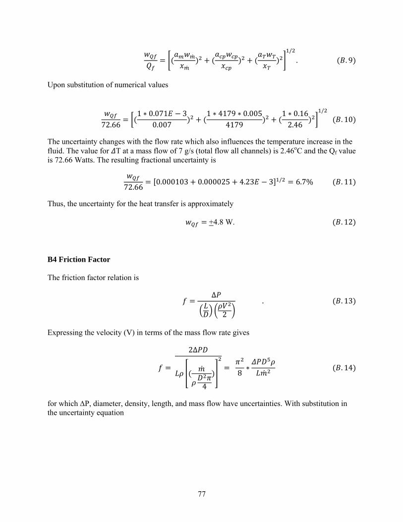
77

Upon substitution of numerical values

The uncertainty changes with the flow rate which also influences the temperature increase in the fluid. The value for T at a mass flow of 7 g/s (total flow all channels) is 2.46oC and the Qf value is 72.66 Watts. The resulting fractional uncertainty is

Thus, the uncertainty for the heat transfer is approximately

+4.8 W.

B4 Friction Factor

The friction factor relation is

Expressing the velocity (V) in terms of the mass flow rate gives

for which P, diameter, density, length, and mass flow have uncertainties. With substitution in the uncertainty equation

78

For the flow conditions associated with 7 g/s (or 0.000636 g/s for a single channel), the variable values are 4184 Pa for P, 0.000635 m for D, 989 kg/m3 for , and 0.02159 m for L. The uncertainty values are 345 Pa for pressure, 1.27*10-5 m for D and L, 0.01 for , and 0.000071 kg/s for the mass flow rate. The result for this evaluation is 0.01477 or a 25% uncertainty (for a nominal f of 0.06). B5 Reynolds Number

The Reynolds number written in terms of the mass flow rate is

where mass flow rate, diameter, and viscosity have uncertainties. The individual uncertainties are 0.000071 kg/s for the mass flow rate, 1.27 x 10-5 m for the diameter, and 1% for the viscosity. The uncertainty equation is

Evaluated partial derivatives give

The resulting uncertainty for ReD is

79

The uncertainty in Re at a flow rate of 7 g/s (total flow all channels) is roughly + 30. B6 Nusselt Number

The convective heat transfer is commonly described in terms of the dimensionless Nusselt (Nu) number.

with

The quantity Q is the total heat transferred to the channels (expected ~80W), A is the channel surface area (11 channels), Ts is the channel surface temperature, and Tm is the mean bulk temperature. Combining Equations B.14 and B.15

The uncertainty in Q (physical) is 6 W, in L it is 1.27*10-5m, in k it is 1% of 0.56 W/mK, and in (Ts-Tm) it is 0.16 oC. Using Eqn. B.1

Using the 7 g/s heat transfer length for L, 11 mm,

80

B7 References

Holman, J. P., Experimental Methods for Engineers, Seventh Edition. McGraw Hill: Boston, 2001.

81

APPENDIX C

CALIBRATION METHODS

The thermocouples, pressure transducers, and the flow meter were calibrated. A load cell is present in the system and typically would be calibrated. However since the load cell had a calibration certificate, it was not calibrated. The platinum resistance thermometer (PRT) (used as a calibrating unit for the thermocouples) calibration was performed by an in house calibration department. In addition, two points were verified in the RZPS Thermal Laboratory: the freeze point and the normal boiling point for a distilled water sample. All curve fit equations were obtained using KaleidaGraph software. C1 Thermocouple Calibration

The equipment for the thermocouple calibration included a Hart Scientific 1502A PRT reader, Hart Scientific 7320 cooler/bath, and Hart Scientific 5628 PRT. The calibration bath contained Dow Corning 200.50 silicone oil. The equipment is shown in Figure C-1. The indicated bath temperature was used as a reference set point only. All calibrations were performed with the Agilent unit set on internal reference compensation. The Agilent unit was operated for at least 30 minutes before any calibrations or testing was performed.

Recording of the thermocouple readings started when the bath temperature reached the expected value. This was monitored by the PRT, and the bath temperature was considered to be at steady-state conditions when a ± 0.1 oC fluctuation per hour was obtained.

The calibration bath had a temperature limit of 150oC, but test temperatures for the stem could possibly reach 200oC. Thus, a different calibration bath was used for the higher temperatures, and it was capable operating safely at 250oC. Trials with the bath showed that linear fits were reliable up to 210oC.

The setup was such that the thermocouples and the PRT were approximately at the center depth of the bath oil. The PRT and loose thermocouples were attached to an external adjustable stand. To hold the copper heater off the bath base, an insulating block of Macor was used. This limited the effects of the steel bath housing from creating a conduction path. This method, however, left the PRT body improperly submerged in the oil. To compensate for the improper level, the entire PRT, bath oil tank, and the thermocouples were covered by a layer of insulation so that the internal chamber air and oil would then be at the same temperature. Figure C-1 shows the insulation that covered the bath. The thermocouples were calibrated in two groups, and the same equipment and method were used for each group.

The thermocouple calibrations were performed with equipment that would be present during the actual experiments (i.e., wire extensions, data acquisition equipment, and connections). There are

82

six thermocouples located in the heater stem made of copper. These thermocouples were calibrated after they were mounted to the stem.

Figure C-1. Photo of Insulation Used to Cover the Bath and Calibration Components to

Reduce Errors Caused by Conduction through the PRT Body

C1.1 Fluid Thermocouples The fluid thermocouples (TC # 13 and 14) at the inlet/exit of the heat exchanger have (1/16 in diameter) stainless-steel sheaths. To allow for quick change and to lower sheath conduction effects, open tipped probes were chosen. Calibration of the fluid thermocouples required a small T between the two thermocouples for a given PRT reading. Since the enthalpy rise was used as the energy balance check, the temperature increase (T) was critical. The fluid thermocouples were calibrated for a small temperature range since the expected fluid temperatures were expected to be in the range 30-35oC. At increments of 3 oC, the thermocouples were calibrated from 14 to 39oC.

Various curves were fit to the thermocouple data. The curves are listed in Table C-1. The residuals of the fit curves were analyzed, and the best fit determined. The best fit was determined to be a linear curve with the standard deviation between them being 0.04oC. The goodness of fit, R2, is 0.99999 and 1 for each fit. The equations for the two thermocouples are (TC 13 inlet fluid)

83

and (TC 14 exit fluid)

The x value is the voltage reading from the Agilent unit. The Agilent unit is set for T-type thermocouples which automatically fits the voltage readings to the standard thermocouple curve with the internal electronic ice point. C1.2 Stem and Miscellaneous Thermocouples

The stem thermocouples are 0.005 in butt welded T-type. The thermocouples are glued into 0.020 in diameter, 0.030 in deep holes (Figure C-2). The thermocouples were secured with Omegabond 1500 oF ceramic epoxy before calibration. Calibrating the thermocouples in place eliminated re-calibration if the thermocouples were broken during installation. Calibration settings were “random” values between 20oC and 142oC for the all thermocouples that would experience temperatures above 40oC (stem, chamber, and body).

Figure C-2. Stem with Thermocouple Holes

Various calibration curves were also fit for these thermocouples, and the best fit was linear (Table C-1). Except for first and last setting, the standard deviation from TC1 to the other five TC‟s (all stem thermocouples) is approximately 0.05oC. The differences among the readings for thermocouples 1-6 were most important (TC 7-12 are for external readings). The lowest R2 value was 0.99999.

84

Table C-1. Curve Fits for Thermocouples 1-12 (Stem, Body, and Chamber)

TC# Linear Fit

1 y = 0.9992x + 0.0748

2 y = 0.9991x + 0.0489

3 y = 0.9986x + 0.0519

4 y = 0.9992x + 0.002

5 y = 1.0066x - 0.2135

6 y = 1.007x - 0.2154

7 y = 1.0057x - 0.046

8 y = 1.0059x - 0.0046

9 y = 1.0064x + 0.0087

10 y = 1.0049x + 0.1155

11 y = 0.9982x + 0.2984

12 y = 0.9976x + 0.3252

The temperature uncertainty due to the voltage resolution of the Agilent unit is 0.1oC. Using the twice the standard deviation of a nominal measurement during calibration, the uncertainty due to calibration error, wcal, is estimated to be 0.08 oC for the fluid thermocouples and 0.1oC for the stem thermocouples. The random error due to voltage fluctuation is estimated to be 0.1oC. To estimate the uncertainty in the thermocouple measurements, the contributions to uncertainty from random error, wrand, instrumentation error, winst, and calibration error, wcal, are combined:

w = (wrand2+ winst

2 + wcal2)1\2

Thus, the overall uncertainty in the temperature for the fluid and stem thermocouples is 0.16oC and 0.17oC, respectively. C2 Pressure Transducer Calibration

Two pressure transducers were calibrated (designated INLET and EXIT) using a portable pressure calibrator (Druck, DPI 610). The unit has an accuracy of 0.025% of full scale (fs) with macro and micro pressure adjustment capabilities. The Druck pressure range was 14.7-300 psia. The transducers (Omega PX303-050A5V) had a range of 0-50 psig with an output voltage of 0.5-5 VDC.

The inlet and exit transducers were calibrated separately using the Druck unit with each having 24 random levels for calibration. Each calibration point was allowed to settle for 30 seconds before recording the voltage output values. The recorded values for each transducer was then averaged for each setting and used for curve fitting. Figure C-3 is a schematic of the setup used for calibration. The calibration fits for the inlet and outlet pressure transducers are

85

Figure C-3. Schematic of Setup for Pressure Transducer Calibration

The uncertainty in the pressure measurement due to the voltage resolution of the Agilent unit is negligible relative to the other uncertainties. Using the twice the standard deviation of a nominal measurement, the uncertainty due to random error, wrand, is estimated to be 0.007 psi for the pressure transducers. The uncertainty in the pressure measurement due to calibration is estimated to be 0.05 psi. To estimate the overall uncertainty in the pressure measurements, the contributions to uncertainty from the random error, wrand and calibration, wcal, are combined:

w = (wrand2 + wcal

2)1\2

Thus, the overall uncertainty in the pressure is estimated to be ~ + 0.05 psi at the 49.0 psi level. C3 Flow Meter Calibration

The flow meter calibrated for the system was an Omega (FTB-9504) precision low flow turbine meter with transmitter (FLSC-61). Before flow calibration could be performed, the transmitter electronics required zeroing. The process involved a frequency generator, DVOM, and an oscilloscope. The adjustment of the transmitter was without issue. Details of the process to set the electronic zero are in the instruction manual for the transmitter.

Druck

Pressure

Tee

Transducer to Calibrate

Druck Transducer

To Agilent

86

The calibration of the flow meter was performed with the unit installed in the test stand so potential effects from other components are taken into account. Figure C-4 shows the calibration setup.

Figure C-4. Flow Meter Calibration Setup Schematic

The flow in the system begins with a pump whose suction hose is submerged in a bucket of distilled water. The water flows from the pump through the filter and heat exchanger to the flowmeter and is collected in a graduated cylinder (1000 mL). The flow was provided by a constant pressure pump (Aquatec DDP 5800). The flowmeter signal was monitored by the Agilent data acquisition unit. On and off flow was controlled by a quick turn ball valve located above the graduated cylinder.

The flow meter was calibrated using mass accumulated with time. Since the temperature of the water entering the test section was controlled to always be the same value (and same density), it it reasonable to calibrate the flow meter to yield a mass flow rate rather than a volumetric flow rate. Each test time was random in the range of 36 to 109 seconds for slow flow rates. For high flow rates (1.4-22 g/s), the cylinder was nearly full. The flow settings used are random by estimating the next setting as falling between the previous flow value and one full turn of the valve. An electronic scale was used to monitor the fluid mass. The flow time was found by reviewing the data files provided by the LabView program that reads and records the Agilent unit values. The mass indicated by the scale and divided by the mass accumulation time gave the mass flow rate corresponding to the voltage reading of the flow meter.

It was found during data analysis that the 1-2 second period required for starting and stopping the flow with the valves provided an error of a few percent. To adjust for the varied flow at the start and end, the time from zero to full flow was used to average the mass flow for that same period.

Filter HX

Pump

Graduated Cylinder

Scale

Flowmeter

Flow Valves

87

The averaged mass was removed from the total flow amount and the time was taken from the total time. Smoother curve fits were then obtained after the correction.

The calibration data was fit with various order curves to find the best fit, and a fifth order polynomial provided the best fit for the mass flow rate:

After the curve accuracies were checked with the manufacturer specifications (0.11% of the flow rate), physical flow checks were performed. Prior problems with flow meter failure warranted the check. The calculated error for the measured flow and the calibration points are shown in Figure C-5. The relatively larger error at low flows is expected to be due to the range of flow frequencies chosen for the transmitter. The selected flow calibration range was slightly too great for these low flow rates. The frequency range chosen was 350-1950 Hz. The error was calculated from an average of 3-4 repeated runs at 2-8 g/s.

Figure C-5. Error Calibration Curves for Voltage to Flow Rate Conversion

The uncertainty due to the voltage resolution of the Agilent unit is negligible relative to the other uncertainties. Using the twice the standard deviation of a nominal measurement (7 g/s), the uncertainty due to random error, wrand, is estimated to be 0.01 g/s. The uncertainty contribution

0

0.5

1

1.5

2

2.5

3

0 2 4 6 8 10

Pe

rce

nt

Erro

r

Flow g/s

88

due to calibration is estimated to be 0.07 g/s. To estimate the uncertainty in the mass flow rate measurements, the contributions to uncertainty from random error, wrand, and calibration error, wcal, are combined:

w = (wrand2 + wcal

2)1\2

Thus, the overall uncertainty in the mass flow rate (at 7 g/s) is estimated to be 0.071 g/s (~1.0%). One significant mistake occurred during initial calibration attempts. The type of flow meter that was used relied on pulse generation which was provided by the passing of a metallic object through a magnetic field. The first flow meter calibrations were performed with tap water to provide an uninterrupted flow of water. This proved to be a bad decision because the level of iron in the water was high enough to cause failure of the flow meter. However, the use of distilled water resolved the issue.

89

APPENDIX D

SYSTEM DIAGRAMS

Figure D-1. Block Diagram of Electronic Cooling Components

Return to Pump/Cooler

TC

P P

Distilled H2O TC

2 3

4

5

6

7

Filter -40micron 2

Heat Exchanger 3

Heater w/Cu heat spreader 4

Voltage and Current Sampling

Shunt - 6

TC–Stem 6 Total

Flow Meter 7

5 Load cell

1

Agilent DAQ

Computer with LabView

Pump/Cooler – Sinusoidal Temp

1 Power Supply Heater

8

9

8 9

Power Supply for Load Cell, Pressure Transducers, and Flow meter

90

APPENDIX E

WIRING SCHEMATIC

Figure E-1. Wiring Map of Electronic Cooling Test Cell

91

APPENDIX F

LABVIEW DATA ACQUISITION PROGRAM

The LabView program is located on computer 01408189 for the electronic cooling experiment and is backed up on a CD. The file name is “Experiment Runs Agilent 34970A Advanced Datalogger”. The LabView program was developed with the help of Victor Tsao. The program was developed to only record. No component control is capable with the designed program. The front screen allows operator input for file names which has a format based on testing parameters. The program also provides real time numerical and graphical outputs viewable by the operator. Values such as power input to the heater, thermocouple readings, pressures, mass flow rate, and load are available on the front screen. The program also allows the operator to adjust the time increment for recording data to a file. Table F-1 gives the channel designation numbers for the experiment instrumentation. Figure F-1 is the front screen view of the LabView program.

Table F-1. Channel Locations in Agilent DAQ Unit for Each Experimental

Instrument

101 Heater Stem TC Position 1 111 Heater Body TC Inner & Upper Position

102 Heater Stem TC Position 2 112 Upper Chamber Air Temperature

103 Heater Stem TC Position 3 113 Heater Exchanger Inlet Fluid Temperature

104 Heater Stem TC Position 4 114 Heater Exchanger Outlet Fluid Temp

105 Heater Stem TC Position 5 115 Fluid Inlet Pressure Transducer

106 Heater Stem TC Position 6 116 Fluid Outlet Pressure Transducer

107 Lower Chamber Air Temperature 117 Cooling Fluid Flowmeter Transducer

108 Heater Body TC Outer & Lower Position 118 Heater Amperage (Shunt)

109 Heater Body TC Outer & Upper Position 119 Load Cell

110 Heater Body TC Inner & Lower Position 120 Heater Voltage

92

Figure F-1. LabView Front Screen View of Control Program

93

APPENDIX G

COPPER MATERIAL QUANTIFICATION (EDAX)

Figure G-1. EDAX (Energy Dispersive X-ray analysis) Quantification of Copper Used to

Manufacture the Heater and Stem

94

NOMENCLATURE

1D One -dimensional

2D Two-dimensional

3D Three-dimensional

a Width of rectangular channel (m)

A Area (m2)

AlN Aluminum nitride

b Height of rectangular channel (m)

CFD Computational fluid dynamics

Cp Constant pressure specific heat (J/kgK)

CTE Coeff. of thermal expansion (1/oC)

D Diameter (m)

Dh Hydraulic diameter (m)

DBC Direct bonded copper DVOM Digital Volt-Ohm meter

f Friction coefficient

F Cross-sectional area (m2)

Gz Graetz number – Re Pr/(x/d)

Gravitational constant (m/s2)

h Convective heat transfer coefficient (W/m2K)

Hc Micro-hardness of Copper (MPa)

HX Heat exchanger

IGBT Insulated Gate Bipolar Transistor

K Pressure loss coefficient

KL Pressure loss coefficient – minor loses

k Thermal conductivity (W/mK)

Mass flow rate (kg/s)

MOSFET Metallic Oxide Semiconductor Field Effect Transistor

Nux Local Nusselt number

NuD Mean Nusselt number based on diameter – hD/k

NuD-x Local Nusselt number

n Area Ratio

P Pressure (Pa)

P Pressure Drop (Pa)

PID Proportional integral derivative

Pr Prandtl Number (cp/k)

Q Heat transfer rate (W)

QS Heat transfer rate through copper stem (W)

q” Heat flux (W/m2)

R Thermal resistance (K/W)

RI Thermal resistance for insulation (K/W)

RA Thermal resistance for air (K/W)

Rc Copper thermal resistance (K/W)

Rf Thermal resistance fluid channel

Re Reynolds number

95

ReD Reynolds number based on diameter (

Re0 Reynolds number for friction factor departure from theory

Re1 Reynolds number for beginning of transition to turbulent flow

Re2 Reynolds number for end of transition to turbulent flow

RTD Resistance thermal device

r* Critical radius

SiC Silicon Carbide

Si Silicon

SiO2 Silicon dioxide

T Temperature (oC or K)

T0 Inlet temperature (TC 1 & 4)

Tc Temperature copper (oC or K)

Tin Bulk temperature channel inlet (oC or K)

Tm Mean fluid temperature (oC or K)

Tout Bulk temperature channel exit (oC or K)

Ts Channel surface temperature (Tw+Tm)/2 (oC or K)

Ttip Temperature stem tip (oC or K)

Tw Temperature channel wall (oC or K)

T Temperature difference (oC or K)

TC Temperature drop across copper stem (oC or K)

TC-F Temperature difference between copper and fluid (oC or K)

TC Thermocouple

u internal energy (J/kg)

V Velocity (m/s)

Vavg Average velocity (m/s)

Vfr Fluid velocity along friction Surface (m/s)

Vloc Local velocity (m/s)

VAC Voltage AC

VDC Voltage DC

x Distancem)

x Change in distance (m)

xsink Distance across sink (m)

x* (x/D)/Re Pr

Thermal Epansion Coefficient

Surface Roughness (m)

Density (kg/m3)

f Dynamic viscosity (N/sm2)

w Dynamic viscosity at a wall (N/sm2)

ζ Coefficient of flow resistance (pressure loss coefficient) P/(Vavg

2/2)

ζ‟loc Coefficient of local flow resistance

ζfr Coefficient of flow resistance of a segment of length L

ζavg Average coefficient of flow resistance