Aerospace Science and Technology 63 (2017) 245–258

Contents lists available at ScienceDirect

Aerospace Science and Technology

www.elsevier.com/locate/aescte

LES study on the shape effect of ground obstacles on wake vortex

dissipation

C.H. John Wang a,b, Dan Zhao a,∗, Jörg Schlüter c, Frank Holzäpfel d, Anton Stephan d

a School of Mechanical and Aerospace Engineering, College of Engineering, Nanyang Technological University, Singapore 639798, Singaporeb Air Traffic Management Research Institute, Nanyang Technological University, Singapore 637460, Singaporec School of Engineering, Deakin University, Geelong, Victoria 3220, Australiad Institute of Atmospheric Physics, Deutsches Zentrum für Luft- und Raumfahrt (DLR), Oberpfaffenhofen 82234, Germany

a r t i c l e i n f o a b s t r a c t

Article history:Received 5 June 2016Received in revised form 26 December 2016Accepted 30 December 2016Available online 4 January 2017

The lingering wake vortex following a landing aircraft has long been a hazard to aviation safety. Previous studies at the German Aerospace Center (DLR) confirmed the effectiveness of applying ground-based obstacles to improve the dissipation of the wake vortex pair by triggering the onset of the vortex bursting by the artificial introduction of shortwave instability. Following the design of the plate line obstacles as proposed by DLR for vortex dissipation, we further investigate the influence of the shape of the ground obstacles on dissipating wake vortex in the present work. The secondary vortex structure, resulting from the interaction between the vortical flow and the obstacle plate, stems from the location of the obstacle and travels outward along the vortex axis, thus spreading instability to the vortex structure along the way. 3D numerical simulations were conducted using Large Eddy Simulation with OpenFOAM solver. The numerical solutions were first compared to the experimental vortex measurement performed in DLR’s Wasser Schleppkanal Göttingen tow-tank. In addition to the baseline setup three different shaped obstacles were numerically tested and compared in the simulation. The numerical results reveal that 50% reduction of the wake dissipation, measured with the circulation of the vortex, was achieved within t∗ = 1.5 compared to t∗ > 4.0 in the absence of ground obstacle. The present study showed that the shape of the obstacles affects the pattern of the secondary vortex structure created, and the resulting drag force acting on the obstacle has a more direct effect on wake dissipation.

© 2017 Elsevier Masson SAS. All rights reserved.

1. Introduction

Wake vortices at flight level would generally descend below the flight path, and eventually dissipate through a combination of Crow and elliptical instability [1]. However, the wake vortex’s trajectory in the vicinity of an airport is bounded by the ground. This limitation could potentially cause the wake vortex to re-bound into the landing corridor. Indeed, wake-encounter events recorded in FAA, NTSB, and NASA database showed that the ma-jority of these events occurred during the approach and landing leg of the flight [2]. To better understand the dissipation mecha-nism of wake vortices near ground, several field studies that mea-sured the strength and trajectory of aircraft wake vortices have been conducted using LIDARs [3–10] or anemometers [11] in the past few decades at selected airports. Additional studies using ei-

* Corresponding author.E-mail address: zhaodan@ntu.edu.sg (D. Zhao).

http://dx.doi.org/10.1016/j.ast.2016.12.0321270-9638/© 2017 Elsevier Masson SAS. All rights reserved.

ther numerical methods [1,6,12–17], ground based experimental works [18–21], or empirical models [22] were also conducted. These studies offered a more controlled environment in order to isolate the influence of various atmospheric effects. Efforts were also made to better analyze and categorize the hazard criterion of wake encounter [23,24].

Previous studies on vortex instability in ground effect haveshown that while it is possible for Crow instability to develop at very low Reynolds number and large initial height (h0 > 10b0), the decay of a counter rotating vortex pair is largely due to the instability from the vortex–ground interaction [1,6,19,20]. Three di-mensional, nonuniform flow separation along the axial direction of the wake vortex would be elongated into streaks as the counter-rotating vortex pair moves away from each other. These streaks would inter-connect and form hairpin like structures, referred to as secondary vortex structure (SVS), that would wrap around the individual wake vortex. The short-wave instability introduced into wake vortex by the SVS would cause local bursting of vortex core,

246 C.H.J. Wang et al. / Aerospace Science and Technology 63 (2017) 245–258

Nomenclature

� Circulation . . . . . . . . . . . . . . . . . . . . . . . . . . . . . . . . . . . . . . . . m2/s�max Circulation calculated with radius that yields

maximum value . . . . . . . . . . . . . . . . . . . . . . . . . . . . . . . . . . m2/sν Kinematic viscosity . . . . . . . . . . . . . . . . . . . . . . . . . . . . . . . m2/sb0 Initial vortex separation . . . . . . . . . . . . . . . . . . . . . . . . . . . . . m

rc Vortex core radius . . . . . . . . . . . . . . . . . . . . . . . . . . . . . . . . . . . mRe� �0/ν Reynolds number based on vortex circulationt0 Vortex descend time based on initial descend speed,

b0/V 0 . . . . . . . . . . . . . . . . . . . . . . . . . . . . . . . . . . . . . . . . . . . . . . . . . sV 0 Initial vortex descend speed . . . . . . . . . . . . . . . . . . . . . . . m/s

leading to the rapid decay of vortex strength throughout the vortex pair.

Ongoing studies of wake vortex near ground at the German Aerospace Center (DLR) showed that the rapid-decay of the wake vortex could be triggered by introducing ground based obstacles [25–28]. The introduction of these obstacles would stretch the sec-ondary vortex created by vortex–ground interaction into a loop shape, the so called � vortex. The � vortex created by the obsta-cles would function similar to the SVS produced by the ground-streak, thus causing accelerated bursting at the location of the obstacles as well as the transmission of the instability along the vortex axis.

2. Previous studies

The idea of introducing obstacles around runway to mitigate the effect of wake vortex on flight safety had been investigated during the past few decades [29]. Foregoing studies were quantitative in nature and focused on either containing the wake vortex pair with the use of barrier plates or disrupting the wake with active devices e.g. suction or blowing fans. The concept introduced in the DLR tow tank experiment [26], on the other hand, focused on the cre-ation of secondary vortex structures using square–cylinder shaped ground obstacle. The experiment was conducted in the 18 m long water filled tow-tank, the Wasser Schleppkanal Göttingen (WSG), with a cross-section of 1.1 m × 1.1 m. The wake vortex was gen-erated by towing a rectangular wing model, with DLR’s F 13 airfoil profile, at 2.44 m/s inside the tank with an initial vortex roll-up height of 0.5b0; the initial vortex height was limited by the model support system and the maximum water level that the experi-ment could be conducted at without spillage. The vortex parameter based on stereo PIV measurement showed that the initial vortex separation b0 is 0.153 m, circulation �0 is 0.052 m2/s, the de-scend speed V 0 is 0.049 m/s, and the core radius rc is 0.009 m; the Reynolds number based on circulation is Re� = 52,000. This Reynolds number is much smaller than the Re� for a full size Air-bus 340, which is 3.42 × 107.

An obstacle with a cross-sectional area of 0.2b0 × 0.2b0 was used in the experiment. It was placed across the channel. Re-sults from the experiment showed that the presence of this ob-stacle could effectively introduce secondary vortex structure. The study showed that the SVS could effectively accelerate the reduc-tion of wake vortex circulation throughout the test domain. Similar speed-up in circulation reduction were observed from the comple-mentary Large Eddy Simulation (LES) investigation conducted at Re� = 23,130.

Refinements to the obstacle to accommodate navigational and flight-safety requirements resulted in the “Plate-Line” type obsta-cle setup. It consisted of an array of thin plates situated prior to the runway and distributed across the landing path. The normal vectors of the plates were perpendicular to the direction of the runway [25–27]. The cross-sectional profile of the obstacles were reduced to 0.1b0 × 0.2b0 in height and width; the plates were placed at 0.45b0 interval. The LES results showed that the sec-ondary vortex structure generated by this setup was similar to the SVS generated by the square cylinder obstacle, and the different se-tups resulted in a similar level of circulation reduction. The lower

Reynolds number of the WSG and LES studies meant that vortex interaction suffered from greater viscous losses to the environment and less severe influence by turbulence on the vortex comparing to flight condition [30]. However, the results from these studies still provided valuable insights on the impact of ground-obstacles on wake vortex dissipation, and formed the basis for subsequent flight experiment conducted by DLR at the Oberpfaffenhofen airport. The flight test showed a clear reduction in wake vortex circulation with the Plate-Line installed comparing to the case without obstacle implementation. By matching the circulation curve and SVS gen-eration pattern of a new obstacle setup to that of the Plate-Line obstacle at WSG Reynolds number range, it is expected that simi-lar performance between the two under flight conditions could be observed. It is therefore one of our goals in the present investiga-tion of ground obstacles to match, if not exceed, the performance of the Plate-Line obstacle at the WSG Reynolds number due to the limitation in computational resources at Nanyang Technolog-ical University.

The current study was based on the “Plate-Line” type obstacles as proposed by DLR, aimed to study the effect of the geometric shape (x–y profile) of the obstacle on the strength and propagation of the instability introduced by the � vortex. The present work is a follow-up study [31]. Detailed information about the solver and the numerical setup is presented in Sect. 3.1 and 3.2, respectively. Four differently shaped obstacles, as described in Sect. 3.4, were numerically tested. Comparison of the present simulation with ex-isting experimental results was made in Sect. 4. The key findings of the current obstacle shape study was summarized and discussed in Sect. 5.

3. Setup of numerical study

3.1. Numerical solver setup

The present simulations were conducted using the open source OpenFOAM library1 [32], in addition, SWAK4FOAM toolbox [33]was used to map the counter rotating vortex pair into the initial velocity field. The numerical solver employed a hybrid Pressure Im-plicit with Splitting of Operator (PISO) and Semi-Implicit Method for Pressure-Linked Equations (SIMPLE) algorithm. However, the PISO only mode was selected for the simulations presented here to avoid the usage of relaxation factors, which enable stable sim-ulation at high Courant number at the cost of time accuracy. The numerical schemes used were linear scheme for interpolation and Gaussian integration. The linear interpolation scheme was used for the calculation of divergence, gradient, and Laplacian, while back-ward time stepping scheme was used for time advancement.

Dynamic Smagorinksy turbulence model implemented in Open-FOAM by Professor Alberto Passalacqua [34] was used in the sim-ulation. It was based on the formulation by Lilly [35] and obtained the Smagorinksy coefficient via cell face averaging. The LES delta used was based on cube-root of cell volume and simple top-hat filter was used for the filter term. Simulation data was logged at

1 Version 2.2.x.

C.H.J. Wang et al. / Aerospace Science and Technology 63 (2017) 245–258 247

Fig. 1. 3D simulation domain defined by initial vortex separation from the DLR study. Schematic from Holzäpfel et al. [26].

t = 0.5 s intervals, which corresponds to t∗ = 0.1.77, due to the limitation in storage space.

The decomposition of the simulation domain was handled using OpenFOAM function. It employed the Simple decomposition algo-rithm, which attempts to create partitions with equal number of grid point in each of the cardinal direction in the order of x, y, and z.

3.2. Simulation domain setup

The simulation domain size was identical in scale as the LES study conducted by DLR for the WSG setup. The non-dimensionalized scale of the simulation domain setup, as pre-sented in Holzäpfel et al. [26], was displayed as Fig. 1.

ANSYS GAMBIT was used for mesh generation. The total cell count for the baseline mesh was chosen based on the mesh used by DLR’s LES study. The baseline mesh was constructed with a 400 ×300× ∼ 100 cells; the final number of cells in the z-direction dependent on the level of refinement for boundary layer mesh. The boundary layer mesh was created using a growth rate of 1.2 start-ing from the first cell height y1 from the wall. It is depended on the mesh setup, with the size of the final cell matching the cell size from the uniform portion of DLR’s mesh scaled by b0.

For mesh generation with obstacles implemented, the boundary layer mesh setup used for the ground was attached to the obstacles in all three directions. Thus, enough resolution was achieved for the flow field around the obstacle as well as the resulting SVS. As a consequence of the wall mesh applied on the obstacles plates, the mesh resolution across the vortex core was significantly higher than the cases without obstacles. Beyond the boundary layer mesh, a small growth rate of 1.01 was imposed on the mesh in all three direction away from the obstacle to reduce the overall number of mesh. The reduction in number of mesh cells was necessary to ensure that the final mesh count is less than 30 million due to the limitation with the available computational infrastructure.

The velocity profile of a single vortex was modeled using the Lamb–Oseen equation. It was based on the previous studies on wake vortex modeling [12–14,17] (Equation (1)) and extruded in the axial direction as given as:

V θ,0(r) = �0

2πr

(1 − exp

(−r2

r2c,0

))(1)

the initial values �0 and rc,0 were listed in Table 1.Also listed in Table 1 were b0, the initial vortex separation,

and t0, the time required for the vortex to drop for a distance of b0 based on initial vortex descend speed V 0. The vortex pair was mapped into the simulation domain at pre-determined height and axial separation by combining the velocity profile of two vor-tices with opposite direction of rotation. It should be noted that

Table 1Variables used to initialize and model aircraft wake vortex based on WSG measurements.

Variable Value

Re� 52,000�0 (m2/s) 0.052rc,0 (m) 0.009b0 (m) 0.153h0 (m) 0.0765V 0 (m/s) 0.043t0 (s) 2.8285

the measured V 0 from WSG was not the same as the value from the equation V 0 = �0/2πb0 for vortex starting from rest. Thus, t0 = V 0/b0 = 2.8285 was used to normalize time in present sim-ulations. All coordinates and lengths were normalized by b0. No background perturbation were used in the present simulations, since previous studies showed that there was no observable dif-ference in circulation between the cases with and without back-ground perturbation.

The lack of initial perturbation led the present simulation result to be simplified to a quasi-2D solution, until 3D instabilities intro-duced by non-uniform vortex–ground separation were developed in the no-obstacle case. When the obstacle plates were present, the 3D perturbation would be introduced by the obstacle–vortex inter-action. This does not seem to affect the circulation measurement. However, the initial solution of the wake vortex in the no-obstacle case could resemble that from a 2D simulation and not reflecting what should be seen in the 3D simulation.

The initial height for the vortex pair was set to h0 = 0.5b0 to reflect the initial vortex height from the WSG experiment. This was in contrast to the typical h0 = b0 setup used wake vortex studies. The difference in the initial height meant that the lateral separation between the wake vortex pair would be smaller com-paring to the typical setup during its interaction with the obstacle plates. This is due to the difference in the trajectory of the counter-rotating vortex pair. It should be noted that the initial wake vortex height of h0 = 0.5b0 was considered very low in wake vortex re-search. It could also indicate that the aircraft was flying below a safe altitude. An elaboration of the glide path and obstacle setup is discussed in Appendix A. The difference between the initial vortex height of h0 = b0 and h0 = 0.5b0 with the square cylinder obstacle was presented in Appendix B.

3.3. Boundary condition setup

No-slip walls (without the use of a wall function, designated as Calculated boundary type in OpenFOAM) was used for velocity boundary condition on the sidewalls in the y-direction, the ground patch, and the obstacles. This is because the flow condition was

248 C.H.J. Wang et al. / Aerospace Science and Technology 63 (2017) 245–258

Fig. 2. The projected x–z area of all obstacles studied except for Obstacle 3.

Fig. 3. Simulation domain with the baseline obstacle (labeled subsequently as seg-Baff) in relation to the orientation and position of the initial vortex pair.

transient, and we were interested in the time accurate flow inter-action near ground. Full slip wall condition (Slip) was used for the top patch. Periodic wall condition (Cyclic) was used on the patches with normal vector in the axial direction (x-direction). This was to avoid velocity gradient at the boundary, which could introduce in-stability into the wake vortex. The usage of the periodic boundary condition on the end walls meant that the setup would actually simulate a series of ground obstacles in the axial (x) direction with a separation of 8b0. The flow field close to these boundaries would not be accurate for the case where only a single set of obstacle plates were employed as discussed later in Sections 4.2 and 5. Zero gradient pressure boundary condition was used for all patches ex-cept for the end-walls, which used periodic boundary condition.

In addition to velocity and pressure field, the implementation of dynamic Smagorinksy model used in the study required the boundary conditions to be defined for turbulent kinetic energy (k) and sub-grid-scale viscosity (nuSgs). On no-slip wall patches k = 0was used. The zero-gradient boundary condition was implemented on the full slip wall patch. The boundary condition for nuSgs were fully resolved (Calculated) for the no-slip wall, and zero-gradient condition was used for the full slip wall patch. As before, the peri-odic boundary condition were used for end-wall patches.

3.4. Geometry of obstacle tested

The obstacles used in this study were based on the design of the “Plate-Line” obstacles as proposed by Holzäpfel et al. [27]. As part of the initial investigation into the capability of OpenFOAM toolbox, a pair of plates, modeled as baffles, each with x–z area of 0.2b0 × 0.2b0 were used, as shown in Fig. 2.

The plates were positioned with its normal aligned with the y-axis. They were placed at 0.5b0 from the y-center-line. In other words, the square cylinder obstacle was removed from the simu-lation domain except for two cross-sectional slices, each at 0.5b0from the y-center-line. The twin-plate setup2 was similar in con-cept to the setup for the Plate-Line obstacle set. It was used as baseline for comparison with all other obstacles. The setup of the baseline obstacles within the simulation domain in relation to the initial vortex pair was shown in Fig. 3.

The purpose of the baseline obstacle test was to show that the solver can handle zero-thickness internal baffles and resolve the associated boundary layer flow. This obstacle configuration evolved from the x–z cross section of the square cylindrical obstacle in the WSG study and the array-of-thin-plates setup from the “Plate-Line” design.

Additional obstacles were proposed with the intention of recon-figuring the plates to produce stronger secondary vortex structure (SVS). This was believed to be the primary mechanism from which instability was introduced into the primary vortex structure. Obsta-cle 1 (chvOut) and 2 (chvIn) were chevron shapes with the opening pointing in opposite orientations with the side-viewed area of the obstacle remained identical to the baseline obstacle. The chevron shape design was thought to promote the formation of stronger and more concentrated SVS along either the outer edge (as in chvOut) or the inner vertex (chvIn) of the obstacles.

On the other hand, the configuration for Obstacle 3 (vortGen) was based on the design of simple counter-rotating vane-type vor-tex generator, which was commonly used to retain boundary layer flow on aerodynamic surfaces. As the primary method of vortex dissipation without the addition of obstacles was from the interac-tion between vortex sheet and ground boundary flow, the usage of vortex generator type obstacle could increase the contact time be-tween the two and ultimately increase the energy dissipated from the wake vortex. The schematics and 3D models for all four obsta-cles investigated in this study was presented in Fig. 4 along with the data label used in later plots.

2 Referred to as segBaff in the subsequent sections.

Fig. 4. Top-down view of the obstacle dimensions used in the current study.

C.H.J. Wang et al. / Aerospace Science and Technology 63 (2017) 245–258 249

Fig. 5. Comparison of circulation data from simulation domain with various mesh density, as represented by the total mesh count.

4. Mesh convergence and comparison with experimental data

4.1. Comparison to experimental data without obstacle

The mesh convergence study was conducted without an obsta-cle at three different mesh refinement levels. They were imple-mented by using three different mesh size for the uniform portion of the mesh. Velocity and pressure data were extracted at x∗ = 0(normalized with b0). The tracking of vortex center and calculation of vortex circulation were done using an in-house code. The loca-tion of the vortex center was tracked by locating the grid point within the search domain with the minimal pressure value. The circulation of the vortex was calculated using � = ˜

Sω · dS with

the measurement area defined by �max = maxr{�(r)} so that the numerical data were comparable with results obtained from the WSG experiment. For the present simulations, the value for rmax

was evaluated at the beginning of the simulation and coincide with �15. It was the circulation calculated using scaled equivalent of r = 15 m, i.e. rmax = 15 × (b0,towtank/b0,full scale) = 0.049 m. Cir-culation magnitude from the two primary vortex structure were averaged for each of the cases discussed below.

A consequence of evaluating the circulation with �max instead of �5−15 is that the circulation curve would raise above �0 dur-ing the vortex diffusion phase. After obtaining the circulation date, comparison was then made with the WSG experimental data from t∗ = 0 to 1. This time period covered the descent of the vortex and its initial contact with the ground, but before formation of SVS due to flow separation in the near ground boundary layer (Fig. 5).

For the simulation time t∗ > 1, the onset of boundary flow separation meant that the resolution of near ground wall mesh be-came important in circulation prediction (Fig. 6). As the wall mesh was defined by the growth rate and last cell length, the y1 values corresponding to the three mesh density used in the mesh con-vergence study are 0.0019. 0.0015, and 0.0003 m. A fourth, more refined wall mesh, was attached to the baseline mesh after initial simulations, as it became apparent that the y1 size from the base-line mesh was insufficiently refined to obtain good agreement to experimental data.

The velocity contour from x∗ = 0 was presented in Fig. 7 for the four y1 values. It showed large near wall velocity drop in the cases where coarser wall mesh was used. Results from the mesh with insufficiently low y1 to resolve the boundary flow showed a jump in velocity from zero, as enforced by the no-slip wall condi-tion, to the calculated velocity at y1 based on linear interpolation and boundary value. The additional flow energy removed due to the lack of resolved or modeled boundary layer flow would con-

Fig. 6. Comparison of circulation data among various boundary mesh size (in me-ters) along the ground.

tribute to the circulation reduction for the coarser mesh as shown in Fig. 6.

Both the vertical (z-direction) and lateral (y-direction) track of the vortex center were recorded from the present simula-tions. However, only the vertical position over time was presented (Fig. 8) as we do not have lateral position data from WSG experi-ments to compare to.

The initial rebound height from the LES vortex trajectory was higher comparing to the WSG data. This phenomenon was similar to what was also observed in the accompanying LES study by DLR using the WSG setup. The difference in initial rebound height be-tween the present LES and WSG data could be due to the lack of background perturbations, which reduced the current simulations to a quasi-2D state. However, similar trajectory was observed in the DLR study, which did account for background turbulence. An-other cause for the difference could be due to the difference in initial vortex profile between ones generated by the towed wing model and the Lamb–Oseen vortex. The lack of background turbu-lence was the likely cause of the difference in trajectory between the two LES results reported. However, the reported circulation val-ues were similar. This was likely due to the short-wave instability introduced by atmospheric turbulence acts on a longer time scale [12,36,37]. Thus, it would require more time to have an observable effect on vortex circulation. Wake vortex dissipation in ground ef-fect, especially with the reduced initial height in the current setup, was dominated by the vortex–ground interaction.

4.2. Comparison to experimental data with obstacle

In additional to the no-obstacle studies, the square cylindrical obstacle setup from the WSG and LES study at DLR [26] was repli-cated in the present simulation. The obstacle consisted of a square cylinder with x–z area of 0.2b0 × 0.2b0 that spanned the entire simulation domain along the y-axis.

With the introduction of the obstacles inside the simulation do-main, it was discovered that the periodic boundary condition used for the end wall3 (located at x∗ = 4) would cause flow features traveling along the vortex axis outward to collide near the bound-ary region, which was similar to the collision at the boundary patch observed for symmetric boundary condition. The outward traveling SVS would collide and “rebound” off SVS originated from an imaginary obstacle set in mirrored position from the patch. The flow pattern close to the end wall thus behaved as if there were infinitely repeating obstacle pairs along the vortex axis in-stead of having just a single set of obstacle(s) as in the case of the towing-tank experiment. The effect of the boundary condition im-plemented at the domain boundary patch in our simulations was

3 Boundary patch normal to the x-axis.

250 C.H.J. Wang et al. / Aerospace Science and Technology 63 (2017) 245–258

Fig. 7. Velocity contour at x∗ = 0 of the vortex–ground interaction with various wall-boundary setup viewing in the x (axial) direction at t∗ = 0.805. (For interpretation of the references to color in this figure, the reader is referred to the web version of this article.)

especially apparent in the circulation plot near the end wall, as shown in Fig. 9(c). Here the colliding SVS would lead to a signifi-cantly faster dissipation and larger reduction in magnitude of wake vortex circulation.

The SVS flow collision at the end wall patch could be the cause for the difference between circulation curve shown in Fig. 9 be-tween the WSG data and the two LES results. Unfortunately, while experiment with two sets of ground obstacles were conducted dur-ing the WSG study, the circulation data was not directly compara-ble with the present simulation result: The dye visualization from the towing tank experiment showed that the bulk of SVS collision occurred away from the center point between the two obstacles in the direction that the wing model was traveling in, thus putting a larger distance between the SVS collision region and the sampling plane located at x∗ = 3.6 from the first obstacle.

The compromise of using periodic boundary condition was made in order to ensure that disturbance to the vortex structure did not appear along the end wall due to momentum lost when

Fig. 8. Comparison of vortex trajectory between DLR water towing tank and NTU LES simulation.

C.H.J. Wang et al. / Aerospace Science and Technology 63 (2017) 245–258 251

Fig. 9. Normalized circulation from the square cylinder type obstacle simulation comparing to experimental data from WSG. Data from the current study is marked as NTU.

subjected to pressure outlet boundary condition. On the other hand, the use of slip wall or symmetry boundary condition would result in similar reflection of SVS at the boundary patch, but with the additional limitation on flow advection across the boundary patch. Ultimately, the usage of periodic boundary condition meant the evaluation of simulation results must be done by comparison to a baseline simulation case to see if the obstacle positively or negatively affected the dissipation of wake vortex.

It could be seen from Fig. 9 that there was a clear difference between the LES results from DLR and the present data set. The difference in circulation result was likely due to several differ-ences in the simulation setup. No initial perturbation were used in the current study. However, a background turbulence field based on wake turbulence of the support strut from the WSG experi-ment was used in the DLR simulation. Additionally, boundary layer mesh was attached to all sides of the obstacle in the current study, whereas it was only applied to the floor patch in the DLR study.

Finally, the Reynolds between the two studies differed by a fac-tor of two, although the difference should not be sufficient to have a noticeable difference in flow condition. A combination of these differences could lead to a more distinct SVS generated with the present setup, resulting in larger circulation reduction from the SVS and faster SVS propagation away from the obstacle. The for-mer showed up as steeper circulation curve in Fig. 9(a), while the later as the earlier drop-off of circulation curve in Fig. 9(b) and 9(c). The difference in circulation curve disappeared after t ∼ 1.5, when the change in circulation was no longer driven by the SVS.

5. Simulation results with different shaped obstacles

The influence of different obstacle shapes on the wake dissi-pation rate was evaluated by calculating the vortex circulation on sampling planes located at x∗ = 0, x∗ = 1.05, and x∗ = 3.6. These locations were chosen based on the availability of WSG experimen-tal data. While the influence of end wall boundary condition on circulation plot had been examined in Sect. 4, the existence of cir-culation data at these locations from previous LES studies allowed us to evaluate the relative effectiveness of the new obstacle de-signs compared to the square cylinder obstacle.

The circulation plot from the result with the baseline (segBaff) obstacle pair was illustrated in Fig. 10. For comparison, the LES and WSG data for the square cylinder obstacle (stdObs) were also plotted. The plot was setup mainly to compare the new obstacle designs proposed in the current study with similar, existing ob-stacle design. The comparison allowed the data from the baseline (segBaff) obstacle simulation to be used in subsequent analysis. This data set would act as the baseline for comparing different obstacle shapes that were proposed.

The circulation plot from Fig. 10 showed that only employing a single pair of baffle type obstacle was less effective at x∗ = 0 and x∗ = 3.6 comparing to the simulation result with the square cylin-der obstacle. The circulation curve for the baseline (segBaff) obsta-cle showed a slightly larger dip at x∗ = 1.05 between t∗ = 0.5∼1.0. However, the circulation magnitude recovered to comparable level with the square cylinder by t∗ = 1.5. The efficiency of a single pair of baffle used for the baseline (segBaff) obstacle was quite remarkable considering the overall size difference between these two obstacles configurations that was compared here. The result complements the finding from DLR’s research into plate-line tech-nology, which showed that multiple plates with lateral (y) sepa-ration of 0.45b0 was able to offer comparable performance of a square cylindrical obstacle but at half of the obstacle height [25].

With the performance of the baseline (segBaff) obstacle act-ing as the baseline, the circulation plot for the obstacles listed in Sect. 3.4 were presented and compared in Fig. 11.

The circulation plots from Fig. 11 showed similar level of vor-tex dissipation across the board in the later part of the simulation for t∗ > 2. However, the intensity of the wake vortex at that point (< 0.4�0) might have only very little effect on the trailing aircraft. A possible explanation for the lack of difference in vortex circula-tion at the later portion of the simulation could be the increased elevation of the vortex core. This led to a greater distance between wake vortex and ground obstacle. Another explanation would be that the vortex lacks the coherency and strength at later time. This resulted in a weaker interaction with the obstacles and thus weaker SVS production.

Despite showing similar circulation level in the later part of simulation, the initial circulation dissipation pattern was quite dis-tinct among the obstacle tested. While identical in height, at x∗ = 0the baseline obstacle (segBaff) and Obstacle 2 (chvIn) caused al-most immediate drop in circulation whereas a time delay was observed for Obstacle 1 (chvOut) and 3 (vortGen). Obstacle 3 (vort-Gen), especially, showed the least effect on vortex circulation until

252 C.H.J. Wang et al. / Aerospace Science and Technology 63 (2017) 245–258

Fig. 10. Normalized circulation from the baseline plate-type obstacle (segBaff) and square cylinder (stdObs) simulation comparing to experimental data from WSG with, and without, the square cylinder obstacle (stdObs).

t∗ ∼ 1.5. This was believed to be due to the upward motion of the vortex structure. The vortex structure would move above the height of the obstacles and away from the influential region of the obstacle, as shown in Fig. 12.

Additionally, the trajectory of the “downwind” vortex4 in the y–z plane at x∗ = 0 (Fig. 13) showed the vortex moving further away from the location of the obstacle, shown in light gray color; the lateral (y) position of the obstacle at t∗ = 0 were the same for all of the different shaped obstacles.

One of the consequences of implementing the obstacles to lined up in lateral (y) position at x∗ = 0 was that the bulk of the ob-stacle structure would be either closer (chvIn) or further away (chvOut) from the domain centerline. From the y–z trajectory from

4 The vortex on the left hand side when viewing in the direction of travel an aircraft.

Fig. 11. Normalized circulation plot of the four obstacle setups listed in Fig. 4.

Fig. 12. Comparison of vortex trajectory from the different obstacles investigated in NTU LES study along with the LES result from simulation without obstacles.

C.H.J. Wang et al. / Aerospace Science and Technology 63 (2017) 245–258 253

Fig. 13. Trajectory of the “downwind” vortex on the y–z plane located at x∗ = 0with the implementation of various obstacles. The thick gray line indicates the lo-cation and height of the obstacle.

Fig. 13, it would appear that the obstacle with the bulk of its struc-

ture closer to the centerline would have less time interacting with

the wake vortex, thus should show a slightly lower dissipation rate than the one further away from centerline. However, vortex circu-lation on top of the obstacles as shown in Fig. 11(a) showed a larger initial circulation decline for the obstacle setup closer to the centerline (chvIn). In order to gain more insight on the flow in-teraction that led to the different circulation curves observed, flow visualization with iso-surface plot for ‖ω∗‖ = 79 was performed.

We can observe the difference in vortex breakup pattern and level or deformation due to SVS in the iso-surface visualizations shown in Fig. 14 and Fig. 15. For example in Fig. 14, SVS gener-ated from the baseline obstacle and Obstacle 1 (chvOut) induced a much larger deformation to the wake vortex structure, indicating a strong radial component for the SVS. On the other hand, Obstacle 2 (chvIn) generated the weakest SVS based on ωy contour. Despite the above stated difference, the trend for circulation reduction was surprisingly similar at the later stages of the simulation (t∗ > 2) for x∗ = 0 and x∗ = 1.05 measurements. This confirmed earlier ob-servation that as the vortex core raise above its initial height, the dissipation rate depended less on the new SVS generated and more on the SVS already intertwined with the wake vortex. In general, the velocity of circulating flow about the vortex core was weaker

Fig. 14. Visualization at t∗ = 0.483, showing iso-surface for ‖ω∗‖ = 79 and the onset of secondary vortex structure looking in the top-down direction. (For interpretation of the references to color in this figure, the reader is referred to the web version of this article.)

254 C.H.J. Wang et al. / Aerospace Science and Technology 63 (2017) 245–258

Fig. 15. Visualization at t∗ = 1.288, showing iso-surface for ‖ω∗‖ = 79 and the onset of secondary vortex structure looking in the top-down direction. (For interpretation of the references to color in this figure, the reader is referred to the web version of this article.)

further away from the vortex core, and would generate weaker SVS that no longer significantly affects the wake vortex.

The iso-surface visualization also allowed us to observe the dif-ference in SVS formation due to the difference in obstacle shape. The SVS formation for the baseline (segBaff) obstacle and Obsta-cle 1 (chvOut) was largely similar to the SVS formation observed with the square cylinder (stdObs) obstacle as reported by Holzäpfel et al. [26]: SVS was initiated at each of the upper corner of the baffle as the flow roll up due to difference in pressure. The SVS creation was similar to the � shaped roll-up of flow along the side walls of the square cylinder (stdObs) obstacle. On the other hand, multiple visible SVS formations were observed in the Obsta-cle 2 (chvIn) and Obstacle 3 (vortGen) simulations. The former saw an additional SVS along the centerline, while the later saw an ad-ditional SVS at each of the exposed inner corner. This could have led to the different wake vortex breakup pattern. However, the dif-

ference did not contribute to significant difference in circulation reduction in the long run (t∗ > 1.5).

One of the more curious observation from the iso-surface plot was the recovery of circulation at x∗ = 0 for the Obstacle 2 (chvIn) case. In this setup, the geometry of the obstacle diverted flow to create a single SVS along the center-line and directing the rest outward in similar fashion as the baseline obstacle as illustrated in Fig. 14 and 15. The recovery in circulation observed could be due to the center-line SVS being ingested back into the primary vortex structure. On the other hand, the accompanying instability introduced into the wake vortex would quickly reduce the over-all circulation down to comparable level with baseline obstacle by t∗ = 1.

Another interesting observation was the recovery at x∗ = 1.05from the baseline obstacle (segBaff) and Obstacle 1 (chvOut). Sim-ilar recovery can be observed in the square cylinder obstacle sim-ulation from both DLR and NTU. The recovery observed between

C.H.J. Wang et al. / Aerospace Science and Technology 63 (2017) 245–258 255

Fig. 16. Vorticity magnitude contour of vortex core at x∗ = 1.05 and t∗ = 0.966 viewing from the x (axial) direction. The white circle indicated area from which the circulation was calculated. (For interpretation of the references to color in this figure, the reader is referred to the web version of this article.)

Fig. 17. Pressure contour of vortex core at x∗ = 1.05 and t∗ = 0.966 viewing from the x (axial) direction. The white circle indicated area from which the circulation was calculated. (For interpretation of the references to color in this figure, the reader is referred to the web version of this article.)

t∗ = 0.7–1.3 could be due to the distortion of vortex shape by the SVS. This resulted in portions of vortex flow falling outside of the circular area which the �∗ data was calculated with; the subse-quent re-integration of distorted flow back into the primary vortex structure lead to the circulation recovery observed in Fig. 11(a). Contour plot for the magnitude of the vorticity presented in Fig. 16illustrated the distortion of vortex core and departure of flow from the core due to the influence of SVS for Obstacle 1 (chvOut) and 2 (chvIn). Here, the dip and recovery of circulation can be observed from the plot for the former and not the later. The pressure con-tour was presented in Fig. 17 for comparison. Note that the circular area, from which the vortex circulation was calculated, was cen-tered at the grid point with the lowest pressure.

The circulation plot from x∗ = 3.6 in Fig. 11(c) was harder to analyze as the rebounding flow would compound to the accelerat-ing of vortex dissipation, although comparison could still be made among the different obstacles due to identical boundary setup. Based on the visualization in Fig. 15, we hypothesize that the lower �∗ number for Obstacle 1 (chvOut) and Obstacle 2 (chvIn) in Fig. 11(c) could be due to stronger SVS with larger momentum away from x∗ = 0 in the axial direction.

Of the four obstacle configurations that were tested, Obstacle 3 (vortGen) proved to be the least effective. It showed the least effect on vortex dissipation, and the difference in circulation reduction

among the obstacles was especially pronounce at x∗ = 0 which was directly on top of the obstacles. Additionally, a noticeable delay in the onset of vortex breakup can be observed for Obstacle 3 (vort-Gen) at x∗ = 0 and x∗ = 3.6 even though the mean lateral position of the obstacle was the same as the baseline obstacle (segBaff).

To better understand the overall trend in circulation dissipation, a domain-wide circulation analysis was conducted along the x-axis. The resulting contour plot of domain-wide circulation over time was shown above in Fig. 18.

The effect of applying periodic boundary condition at the end wall is evident in the darkened region near x∗ = ‖4‖. It showed the colliding flow near the periodic wall appearing as early as t∗ ∼ 0.8. The onset of rapid decay phase of vortex evolution, trig-gered by the spreading of SVS outward, can also be observed along the interface between the lighter and the darker region of the con-tour plots. Estimating the traveling speed of SVS can be tricky due to the coarse time resolution, which was limited by the compu-tational hardware. However, a general idea of the SVS spreading speed could still be observed from the plot. The shallower the slope of an interface was, the faster the SVS spreading speed was. The faster traveling SVS from Obstacle 1 (chvOut) and Obstacle 2 (chvIn) could lead to higher energy dissipation near the periodic boundary, resulting in the lower circulation observed in Fig. 11(c).

256 C.H.J. Wang et al. / Aerospace Science and Technology 63 (2017) 245–258

Fig. 18. Visualization of circulation as illustrated by the color scale with respect to normalized time and normalized axial position. (For interpretation of the references to color in this figure, the reader is referred to the web version of this article.)

The domain-wide circulation results suggested that the form drag of the obstacle design could be the major contributor towards the dissipation of wake vortex at x∗ = 0, while SVS played a sec-ondary role. This can be illustrated by contracting the circulation plot (Fig. 18) and drag data (Fig. 19) from Obstacle 1 (chvOut) and 3 (vortGen). The two setups shared similar geometry setup that re-sulted in similar circulation pattern. However, Obstacle 1 (chvOut) had a larger frontal area (view from the y-direction) comparing to Obstacle 3 (vortGen) that resulted in the larger drag force pro-duced.

6. Conclusions

In this work, 3D Numerical studies of the effect of different ob-stacle shapes on wake vortex dissipation were carried out with Large Eddy Simulation using OpenFOAM solver at Re� = 52,000. The variation of vortex strength over time was determined by cal-culating the circulation about the vortex center, �max. The vortex dissipation was characterized through plotting �max against time and visualizing with the magnitude of vorticity (‖ω∗‖) iso-surface. The dimensions of the modeled obstacles are based on the “Plate-line” obstacle proposed by the German Aerospace Institute (DLR). However, for simplicity only a single pair of ground obstacle was used to better isolate the influence on wake dissipation by chang-ing obstacle shape. It was found that implementing a single baffle pair leads to the time for circulation to reach 50% of initial value being reduced to t∗ = 1.5, in comparison to t∗ = 4 in the absence of obstacles. The present results also revealed that the wake dissi-pation rate was related to the shape of the obstacles, especially on top of the obstacles. The obstacle with a shape producing higher drag was observed with faster dissipation (see the difference be-tween Obstacle 1 (chvOut) and Obstacle 3 (vortGen)). Away from the obstacle, the shape of the obstacle appears to affect the forma-

Fig. 19. Y-directional forces as experienced by the obstacle plates throughout the simulation. Note that the force curve for the chvOut obstacle was likely truncated due to coarse time resolution.

tion and strength of secondary vortex structure (SVS) in the axial direction. However, current simulation showed no major distinc-tion in long-term wake dissipation among different SVS patterns that were observed. Moreover, comparison with the results ob-tained in the absence of ground obstacles revealed that the pres-ence of SVS was a major contributor towards increased dissipation of wake vortex. Further study with higher spatial granularity, bet-ter end-wall treatment, or larger computational domain is needed to better understand how different SVS patterns resulted in similar wake vortex dissipation rates.

Conflict of interest statement

The authors declare no conflict of interest.

C.H.J. Wang et al. / Aerospace Science and Technology 63 (2017) 245–258 257

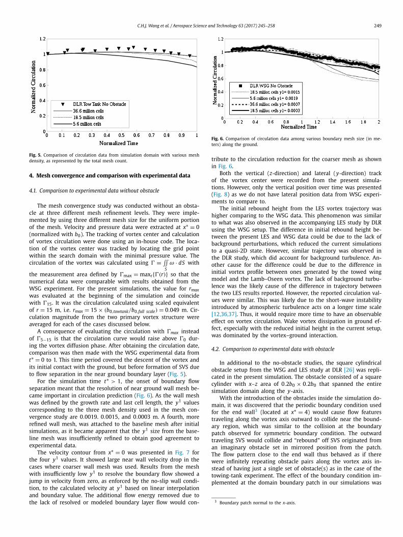
Fig. A.20. The aircraft glide path as enforced by ILS, which has a glide slope of 3◦ and lower bound of 2.5◦ . Also shown are the inner approach surface of the aerodrome (2◦), which defined the maximum height an obstacle can be at around the airport, and the position of the obstacle such that the top left (closer to the runway) corner of the plate is within the height limit.

Acknowledgements

This work was supported by Air Traffic Management Research Institute (ATMRI), and the German Aerospace Center (DLR) under grant number M4061216.056. This financial support was gratefully acknowledged. We would like to thank Dr. Thomas Gerz for his feedback, support, and holding the research visit in DLR last year. The provision of the towing tank data by Reinhard Geisler and Robert Konrath of the Institut für Aerodynamik und Strömung-stechnik, Deutsches Zentrum für Luft- und Raumfahrt (DLR) in Göttingen is greatly acknowledged.

Appendix A. Initial wake vortex height based on glide slope

The initial height of the wake vortex for a simplified landing situation was calculated based on the obstacle placement. It was limited by the aerodrome obstacle restriction as well as the min-imum runway end safety area (RESA, 90 meters from the end of runway) issued by ICAO [38]. Note that the obstacles would need to be further away from the runway if the ICAO recommended RESA of 240 m from the end of runway is used. The numbers and schematic presented in Fig. A.20 were calculated based on the assumption that the wake vortex was generated by a widebody aircraft that followed the glide path identified by the Instrument Landing System (ILS). Note that flaring of the aircraft was not ac-counted for in the calculation, since it occurred right before touch-down, and should have little impact on the aircraft height above the obstacle. The numbers below the different obstacle setup were the height of the glide path center line, glide path lower bound, and the obstacle restriction height directly above the center-point of the obstacle.

Appendix B. Effect of initial wake vortex height on simulation result

The purpose of this Appendix is to illustrate the difference between the present simulation results from the square cylinder (stdObs) case that employed initial vortex height of h0 = 0.5b0 and h0 = b0. Fig. B.22 showed the vortex trajectory from each of the cases, with the h0 = b0 case showing the vortices diverging from each other at z ∼ 0.7b0, a typical behavior observed in counter-rotating vortex pair. The circulation plots shown in Fig. B.21 offset the h0 = 0.5b0 data by t∗ = 0.6, which was the time it took for the vortex with higher initial height to descend to 0.5b0 above ground. The difference in circulation reduction from SVS was likely due to the different distance between the vortex trajectory and the obsta-cle: The shorter distance between the vortex core and obstacle for the h0 = 0.5b0 case meant that the vortical flow would impact the obstacle at higher angular velocity, thus creating a stronger SVS and a steeper slope in the circulation plot. The circulation curve for the two cases were similar after the generation of SVS ceased.

Fig. B.21. Circulation plots comparing the difference between wake vortex with dif-ferent initial height.

Fig. B.22. The “downwind” vortex trajectory from the square cylinder (stdObs) ob-stacle case with different initial vortex height at x∗ = 0. The blue line identified the upper edge of the square cylinder obstacle. (For interpretation of the references to color in this figure legend, the reader is referred to the web version of this article.)

258 C.H.J. Wang et al. / Aerospace Science and Technology 63 (2017) 245–258

References

[1] T. Leweke, S. Le Dizés, C. Williamson, Dynamics and instabilities of vortex pairs, Annu. Rev. Fluid Mech. 48 (1) (2016) 1–35.

[2] P. Veillette, Data showed us wake-turbulence accidents are most frequent at low altitude and during approach and landing, in: Flight Safety Digest, 2002, pp. 1–47.

[3] R. Huffaker, A. Jelalian, J. Thomson, Laser Doppler system for detection of air-craft trailing vortices, Proc. IEEE 58 (3) (1970) 322–326.

[4] S. Campbell, T. Dasey, R. Freehart, R. Heinrichs, M. Matthews, G. Perras, 1995 wake vortex testing program at Memphis, TN, in: AIAA 34th Aerospace Sci-ences Meeting and Exhibit, Reno, NV, USA, 1996.

[5] S. Campbell, T. Dasey, R. Freehart, R. Heinrichs, M. Matthews, G. Perras, G. Rowe, Wake Vortex Field Measurements Program at Memphis, Tennessee – Data Guide, Tech. Rep. CR-201690, NASA, 1997.

[6] P. Meunier, S. Le Dizès, T. Leweke, Physics of vortex merging, C. R. Phys. 6 (4–5) (2005) 431–450, http://dx.doi.org/10.1016/j.crhy.2005.06.003.

[7] D. Nguyen, Wake Vortex JFK2 Final Report: May 26–June 6, 1997 JFK2 Deploy-ment: Wake Vortex Measurements at John F. Kennedy International Airport for a 2.02 mm Pulsed Coherent Lidar, a 10.6 mm Continuous Wave Lidar, and a Ground Wind Vortex Sensing System, Tech. Rep. RTI/4903-032-03S, Research Triangle Institute, 1998.

[8] D. Nguyen, C. Britt, Wake Vortex Lidar, Nasa Lidar 1997 Dallas/Fort Worth Field Measurements and Data Guide, Tech. Rep. RTI/4903-032-04, Research Triangle Institute, 1998.

[9] L. Gardoz, D. Lawrence, N. Miller, The Measurements of the Boeing 747 Trailing Vortex System Using the Tower Fly-by Technique, Tech. Rep. FAA-RD-73-156, Federal Aviation Administration, 1973.

[10] F. Holzäpfel, M. Steen, Aircraft wake-vortex evolution near ground proximity: analysis and parametrization, AIAA J. 45 (1) (2007) 218–227.

[11] D. Burnham, J. Hallock, Measurements of wake vortices interacting with the ground, J. Aircr. 42 (5) (2005) 1179–1187.

[12] F. Holzäpfel, T. Gerz, R. Baumann, The turbulent decay of trailing vortex pairs in stably stratified environments, Aerosp. Sci. Technol. 5 (2001) 95–108.

[13] T. Gerz, F. Holzäpfel, D. Darracq, Commercial aircraft wake vortices, Prog. Aerosp. Sci. 38 (2002) 181–208.

[14] F. Holzäpfel, T. Hofbauer, D. Darracq, H. Moet, F. Garnier, C.F. Gago, Analysis of wake vortex decay mechanisms in the atmosphere, Aerosp. Sci. Technol. 7 (4) (2003) 263–275, http://dx.doi.org/10.1016/S1270-9638(03)00026-9.

[15] F. Proctor, Numerical simulation of wake vortices measured during the Idaho falls and Memphis field programs, in: 14th Applied Aerodynamics Conference, New Orleans, LA, USA, 1996.

[16] A. Corjon, T. Poinsot, Behavior of wake vortices near ground, AIAA J. 35 (5) (1997) 849–855.

[17] F. Proctor, N. Ahmad, F. Duparcmeur, D. Jacob, Review of idealized aircraft wake vortex models, in: 52nd Aerospace Science Meeting, National Harbor, MD, USA, 2014.

[18] L. Jacquin, D. Fabre, D. Sipp, V. Theofilis, H. Vollmers, Instability and unsteadi-ness of aircraft wake vortices, Aerosp. Sci. Technol. 7 (8) (2003) 577–593.

[19] A. Allen, C. Breitsamter, Experimental investigation of counter-rotating four vor-tex aircraft wake, Aerosp. Sci. Technol. 13 (2–3) (2009) 114–129.

[20] C. Breitsamter, Wake vortex characteristics of transport aircraft, Prog. Aerosp. Sci. 47 (2011) 89–134.

[21] O. Elsayed, A. Omar, W. Asrar, K. Kwon, Effect of differential spoiler settings (dss) on the wake vortices of a wing at high-lift-configuration (hlc), Aerosp. Sci. Technol. 15 (7) (2011) 555–566.

[22] T. Sarpkaya, New model for vortex decay in the atmosphere, J. Aircr. 37 (1) (2000) 53–61.

[23] R. Luckner, G. Höhne, M. Fuhrmann, Hazard criteria for wake vortex encounters during approach, Aerosp. Sci. Technol. 8 (8) (2004) 673–687.

[24] F. Holzäpfel, K. Dengler, T. Gerz, C. Schwarz, Prediction of dynamic pairwise wake vortex separations for approach and landing, in: 3rd Atmospheric and Space Environments Conference, Honolulu, HI, USA, 2011.

[25] A. Stephan, F. Holzäpfel, T. Misaka, Aircraft wake-vortex decay in ground proximity-physical mechanisms and artificial enhancement, J. Aircr. 50 (4) (2013) 181–208.

[26] A. Stephan, F. Holzäpfel, T. Misaka, R. Geisler, K. Konrath, Enhancement of air-craft wake vortex decay in ground proximity: experiment versus simulation, CEAS Aeronaut. J. 5 (2) (2014) 109–125.

[27] F. Holzäpfel, A. Stephan, S. Körner, T. Misaka, Wake vortex evolution during approach and landing with and without plate lines, in: 52nd Aerospace Science Meeting, National Harbor, MD, USA, 2014.

[28] A. Stephan, F. Holzäpfel, T. Misaka, Hybrid simulation of wake-vortex evolution during landing on flat terrain and with plate line, Int. J. Heat Fluid Flow 49 (2014) 18–27.

[29] R. Kohl, Model Experiments to Evaluate Vortex Dissipation Devices Proposed for Installation on or Near Aircraft Runways, Tech. Rep. CR-132365, NASA, 1973.

[30] D. Bushnell, G. Greene, High-Reynolds-number test requirements in low-speed aerodynamics, in: High-Reynolds-Number Flow with Liquid and Gaseous He-lium, Springer-Verlag, 1991.

[31] C.J. Wang, J. Schlüter, Near ground aircraft wake dissipation with obstacles, in: 33rd Applied Aerodynamics Conference, Dallas, TX, USA, 2015.

[32] The OpenFOAM Foundation, Openfoam-2.2.x, http://github.com/OpenFOAM/OpenFOAM-2.2.x (commits on 4 January 2015).

[33] The OpenFOAM® extend project, maintained by Bernhard Gschaider, Swiss army knife for foam version 0.2.4, http://sourceforge.net/p/openfoam-extend/swak4Foam (obtained on 22 January 2014).

[34] A. Passalacqua, Implementation of the dynamic Smagorinsky sgs model as proposed by Lilly (1992) for openfoam, https://github.com/AlbertoPa/dynamicSmagorinsky (commits on 2 April 2014).

[35] D.K. Lilly, A proposed modificaiton of the Germano subgrid-scale closure method, Phys. Fluids A 4 (3) (1992).

[36] T. Leweke, S. Le Dizés, C. Williamson, Cooperative elliptic instability of a vortex pairs, J. Fluid Mech. 360 (1998) 85–119.

[37] k. Nomura, H. Tsutsui, D. Mahoney, J. Rottman, Short-wave instability and de-cay of a vortex pair in stratified fluid, J. Fluid Mech. 553 (2006) 283–322.

[38] ICAO Annex 14 – Volume 1: Aerodromes – Aerodrome Design and Operations, 6th edition, International Civil Aviation Organization, 2013.