Embed Size (px)
Citation preview

Provisional chapter
Aeroelasticity of Wind Turbines Blades UsingNumerical Simulation
Drishtysingh Ramdenee, Adrian Ilinca andIon Sorin Minea
Additional information is available at the end of the chapter
http://dx.doi.org/10.5772/52281
1. Introduction
With roller coaster traditional fuel prices and ever increasing energy demand, wind energyhas known significant growth over the last years. To pave the way for higher efficiency andprofitability of wind turbines, advances have been made in different aspects related to thistechnology. One of these has been the increasing size of wind turbines, thus rendering thewind blades gigantic, lighter and more flexible whilst reducing material requirements andcost. This trend towards gigantism increases risks of aeroelastic effects including dire phe‐nomena like dynamic stall, divergence and flutter. These phenomena are the result of thecombined effects of aerodynamic, inertial and elastic forces. In this chapter, we are present‐ing a qualitative overview followed by analytical and numerical models of these phenomenaand their impacts on wind turbine blades with special emphasize on Computational FluidDynamics (CFD) methods. As definition suggests, modeling of aeroelastic effects require thesimultaneous analysis of aerodynamic solicitations of the wind flow over the blades, theirdynamic behavior and the effects on the structure. Transient modeling of each of these char‐acteristics including fluid-structure interaction requires high level computational capacities.The use of CFD codes in the preprocessing, solving and post processing of aeroelastic prob‐lems is the most appropriate method to merge the theory with direct aeroelastic applicationsand achieve required accuracy. The conservation laws of fluid motion and boundary condi‐tions used in aeroelastic modeling will be tackled from a CFD point of view. To do so, thechapter will focus on the application of finite volume methods to solve Navier-Stokes equa‐tions with special attention to turbulence closure and boundary condition implementation.Three aeroelastic phenomena with direct application to wind turbine blades are then stud‐ied using the proposed methods. First, dynamic stall will be used as case study to illustrate
© 2012 Ramdenee et al.; licensee InTech. This is an open access article distributed under the terms of theCreative Commons Attribution License (http://creativecommons.org/licenses/by/3.0), which permitsunrestricted use, distribution, and reproduction in any medium, provided the original work is properly cited.
the traditional methodology of CFD aeroelastic modeling: mathematical analysis of the phe‐nomenon, choice of software, computational domain calibration, mesh optimization and tur‐bulence and transition model validation. An S809 airfoil will be used to illustrate thephenomenon and the obtained results will be compared to experimental ones. The diver‐gence will be then studied both analytically and numerically to emphasize CFD capacity tomodel such a complex phenomenon. To illustrate divergence and related study of eigenval‐ues, an experimental study conducted at NASA Langley will be analyzed and used for com‐parison with our numerical modeling. In addition to domain, mesh, turbulence andtransition model calibration, this case will be used to illustrate fluid-structure interactionand the way it can be tackled in numerical models. Divergence analysis requires the model‐ing of flow parameters on one side and the inertial and structural behavior of the blade onthe other side. These two models should be simultaneously solved and continuous exchangeof data is essential as the fluid behavior affects the structure and vice-versa.
This chapter will conclude with one of the most dangerous and destructive aeroelastic phe‐nomena – the flutter. Analytical models and CFD tools are applied to model flutter and theresults are validated with experiments. This example is used to illustrate the application ofaeroelastic modeling to predictive control. The computational requirements for accurate aer‐oelastic modeling are so important that the calculation time is too large to be applied for realtime predictive control. Hence, flutter will be used as an example to show how we can useCFD based offline results to build Laplacian based faster models that can be used for predic‐tive control. The results of this model will be compared to experiments.
2. Characteristics of aeroelastic phenomena
Aeroelasticity refers to the science of the interaction between aerodynamic, inertial and elas‐tic effects. Aeroelastic effects occur everywhere but are more or less critical. Any phenomen‐on that involves a structural response to a fluid action requires aeroelastic consideration. Inmany cases, when a large and flexible structure is submitted to a high intensity variableflow, the deformations can be very important and become dangerous. Most people are fa‐miliar with the “auto-destruction” of the Tacoma Bridge. This bridge, built in WashingtonState, USA, 1.9 km long, was one of the longest suspended bridges of its time. The bridgeconnecting the Tacoma Narrows channel collapsed in a dramatic way on Thursday, Novem‐ber 7, 1940. With winds as high as 65-75 km/h, the oscillations increased as a result of fluid-structure interaction, the base of Aeroelasticity, until the bridge collapsed. Recorded videosof the event showed an initial torsional motion of the structure combined very turbulentwinds. The superposition of these two effects, added to insufficient structural dumping, am‐plified the oscillations. Figure 1 below illustrates the visual response of a bridge subject toaeroelastic effects due to variable wind regimes. The simulation was performed using multi‐physics simulation on ANSYS-CFX software. Some more details on similar aeroelastic mod‐elling can be viewed from [1], [2], [3] and [4].
Advances in Wind Power2

Figure 1. Aeroelastic response of a bridge
In an attempt to increase power production and reduce material consumption, wind tur‐bines’ blades are becoming increasingly large yet, paradoxically, thinner and more flexible.The risk of occurrence of damaging aeroelastic effects increases significantly and justifies theefforts to better understand the phenomena and develop adequate design tools and mitiga‐tion techniques. Divergence and flutter on an airfoil will be used as introduction to aeroelas‐tic phenomena. When a flexible structure is subject to a stationary flow, equilibrium isestablished between the aerodynamic and elastic forces (inertial effects are negligible due tostatic condition). However, when a certain critical speed is exceeded, this equilibrium is dis‐rupted and destructive oscillations can occur. This is illustrated with Figure 2 where α is theangle of attack due to a torsional movement as a result of aerodynamic solicitations.
Figure 2. Airfoil model to illustrate aerodynamic flutter
If we consider an angle of attack sufficiently small such that cosα ≈1 and sinα≈ α, and writ‐ing the equilibrium of the moments, M, with respect to the centre of the rotational spring,we have:
∑M=0
Le + Wd – Kαα=0 (1)
Where the lift L is:
L = qSCl =qSM0α (2)
S, surface area of the profile, Cl is the lift coefficient, M0 is the moment coefficient. This leadsto an angle of attack at equilibrium corresponding to:
Aeroelasticity of Wind Turbines Blades Using Numerical Simulationhttp://dx.doi.org/10.5772/52281
3

α= WdKα - qSM0e
(3)
For a zero flow condition, the angle of attack αz, is such that:
αz = WdKα
(4)
Divergence occurs when denominator in equation (3) becomes 0 and this corresponds to adynamic pressure, qD expressed as:
qD =Kα
eSM0(5)
Therefore:
α=αz
1 - ( qqD
) (6)
When velocity increases such that dynamic pressure q approaches critical dynamic pressureqD, the angle of attack dangerously increases until a critical failure value – divergence. Thisis solely a structural response due to increased aerodynamic solicitation due to fluid-struc‐ture interaction. This is an example of a static aeroelastic phenomenon as it involves no vi‐bration of the airfoil. Flutter is an example of a dynamic aeroelastic phenomenon as it occurswhen structure vibration interacts with fluid flow. It arises when structural damping be‐comes insufficient to damp aerodynamic induced vibrations. Flutter can appear on any flexi‐ble vibrating object submitted to a strong flow with positive retroaction between flowfluctuations and structural response. When the energy transferred to the blade by aerody‐namic excitation becomes larger than the normal dynamic dissipation, the vibration ampli‐tude increases dangerously. Flutter can be illustrated as a superposition of two structuralmodes – the angle of attack (pitch) torsional motion and the plunge motion which character‐ises the vertical flexion of the tip of the blade. Pitch is defined as a rotational movement ofthe profile with respect to its elastic center. As velocity increases, the frequencies of theseoscillatory modes coalesce leading to flutter phenomenon. This may start with a rotation ofthe blade section (at t=0 s in Figure 3). The increased angle amplifies the lift such that thesection undertakes an upward vertical motion. Simultaneously, the torsional rigidity of thestructure recoils the profile to its zero-pitch condition (at t=T/4 in Figure 3). The flexion ri‐gidity of the structure tends to retain the neutral position of the profile but the latter thentends to a negative angle of attack (at t = T/2 in Figure 3). Once again, the increased aerody‐namic force imposes a downward vertical motion on the profile and the torsional rigidity ofthe latter tends to a zero angle of attack. The cycle ends when the profile retains a neutralposition with a positive angle of attack. With time, the vertical movement tends to damp outwhereas the rotational movement diverges. If freedom is given to the motion to repeat, therotational forces will lead to blade failure.
Advances in Wind Power4

Figure 3. Illustration of flutter movement
3. Mathematical analytical models
Several examples of aeroelastic phenomena are described in the scientific literature. When itcomes to aeroelastic effects related to wind turbines, three of the most common and direones are dynamic stall, aerodynamic divergence and flutter. In this section, we will providea summarized definition of these aeroelastic phenomena with associated mathematical ana‐lytical models. Few references related to analytic developments of aeroelastic phenomenaare [10], [11] and [12].
3.1. Dynamic stall
In fluid dynamics, the stall is a lift coefficient reduction generated by flow separation on anairfoil as the angle of attack increases. Dynamic stall is a nonlinear unsteady aerodynamiceffect that occurs when there is rapid change in the angle of attack that leads vortex shed‐ding to travel from the leading edge backward along the airfoil [14]. The analytical develop‐ment of equations characterizing stall will be performed using illustrations of Figures 4 and5. The lift per unit length, expressed as L is given by:
L = cL12 ρV 2c (7)
Where
• cL is the lift coefficient
• ρ is the air density• c is the chord length of the airfoil
Figure 4. Illustration of an airfoil used for analytical development of stall related equations
Aeroelasticity of Wind Turbines Blades Using Numerical Simulationhttp://dx.doi.org/10.5772/52281
5

We will, first, present static stall as described in [13]. During stationary flow conditions, noflow separation occurs and the lift, L, acts approximately at the quarter cord distance fromthe leading edge at the pressure (aerodynamic) centre. For small values of α, L varies linear‐ly with α. Stall happens at a critical angle of attack whereby the lift reaches a maximum val‐ue and flow separation on the suction side occurs.
Figure 5. Lift coefficient under static and dynamic stall conditions (dashed line for steady conditions, plain line for un‐steady conditions)
For unsteady conditions, a delay exists prior to reaching stability and is an essential condi‐tion for building analytical stall models [15]. In such case, we can observe a smaller lift foran increasing angle of attack (AoA) and a larger one for decreasing AoA when comparedwith a virtually static condition. In a flow separation condition, we can observe a more sig‐nificant delay which expresses itself with harmonic movements in the flow which affects theaerodynamic stall phenomenon. Figure 5, an excerpt from [16], shows that for harmonic var‐iations of the AoA between 0o and 15o,, the onset of stall is delayed and the lift is considera‐bly smaller for the decreasing AoA trend than for the ascending one. Hence, as expressed byLarsen et al. [17], dynamic stall includes harmonic motion separated flows, including forma‐tion of vortices in the vicinity of the leading edge and their transport to the trailing edgealong the airfoil. Figures 6-9, which are excerpts from [18], illustrate these phenomena.
Figure 6. Aerodynamic stall mechanism- Onset of separation on the leading edge
Advances in Wind Power6

Figure 7. Aerodynamic stall mechanism- Vortex creation at the leading edge
Figure 8. Aerodynamic stall mechanism- Vortex separation at the leading edge and creation of vortices at the trailingedge
Figure 9. Aerodynamic stall mechanism – Vortex shedding at the trailing edge
Aeroelasticity of Wind Turbines Blades Using Numerical Simulationhttp://dx.doi.org/10.5772/52281
7

Stall phenomenon is strongly non-linear such that a clear cut analytical solution model isimpossible to achieve. This complex phenomenon requires consideration of numerous pa‐rameters, study of flow transport, boundary layer analysis (shape factor and thickness), vor‐tex creation and shedding as well as friction coefficient consideration in the boundary layer.The latter helps in the evaluation of separation at the leading edge and is important for aer‐oelastic consideration. The proper modelling of transition from laminar to turbulent flow isalso essential for accurate prediction of stall parameters.
3.2. Divergence
We consider a simplified aeroelastic system of the NACA0012 profile to better understandthe divergence phenomenon and derive the analytical equation for the divergence speed.Figure 10 illustrates a simplified aeroelastic system, the rigid NACA0012 profile mountedon a torsional spring attached to a wind tunnel wall. The airflow over the airfoil is from leftto right. The main interest in using this model is the rotation of the airfoil (and consequenttwisting of the spring), α, as a function of airspeed. If the spring were very stiff and/or air‐speed very slow, the rotation would be rather small; however, for flexible spring and/orhigh flow velocities, the rotation may twist the spring beyond its ultimate strength and leadto structural failure.
Figure 10. Simplified aeroelastic model to illustrate divergence phenomenon
The airspeed at which the elastic twist increases rapidly to the point of failure is called thedivergence airspeed, U D. . This phenomenon, being highly dangerous and prejudicial forwind blades, makes the accurate calculation of U D very important. For such, we define C asthe chord length and S as the rigid surface. The increase in the angle of attack is controlledby a spring of linear rotation attached to the elastic axis localized at a distance e behind theaerodynamic centre. The total angle of attack measured with respect to a zero lift positionequals the sum of the initial angle αr and an angle due to the elastic deformation θ, knownas the elastic twist angle.
α = αr + θ (8)
The elastic twist angle is proportional to the moment at the elastic axis:
Advances in Wind Power8
θ =C θθT (9)
where C θθ is the flexibility coefficient of the spring. The total aerodynamic moment with re‐spect to the elastic axis is given by:
T =(Cle + Cmc)qS (10)
where
• Cl is the lift coefficient
• Cm is moment coefficient
• q is the dynamic pressure• S is the rigid surface area of the blade section
The lift coefficient is related to the angle of attack measured with respect to a zero lift condi‐tion as follows:
Cl =∂Cl
∂α (αr + θ) (11)
Here ∂Cl
∂α represents the slope of the lift curve. The elastic twist angle θ, can be obtained bysimple mathematical manipulations of the three previous equations:
T =∂Cl
∂α (αr + θ).e + Cmc qS (12)
Hence,
θ =C θθ ∂Cl
∂α (αr + θ).e + Cmc qS (13)
θ =C θθ ∂Cl
∂α αreqS +∂Cl
∂α θeqS + CmcqS (14)
Regrouping θ :
θ 1 -∂Cl
∂α C θθeqS =C θθ ∂Cl
∂α αreqS + CmcqS (15)
This leads to:
θ =C θθ∂ Cl∂ α αr eqS + CmcqS
1 -∂ Cl∂ α C θθeqS
(16)
Aeroelasticity of Wind Turbines Blades Using Numerical Simulationhttp://dx.doi.org/10.5772/52281
9

We can note that for a given value of the dynamic pressure q, the denominator tends to zerosuch that the elastic twist angle will then tend to infinity. This condition is referred to as aer‐odynamic divergence. When the denominator tends to zero:
1 -∂Cl
∂α C θθeqS =0 (17)
The dynamic pressure is given by:
q = 12 ρv 2 (18)
Thus, we come up with:
1 -∂Cl
∂α C θθe 12 ρv 2S =0 (19)
Hence, the divergence velocity can be expressed as:
U D = 1
C θθ∂ Cl∂ α e
12 ρS
(20)
To calculate the theoretical value of the divergence velocity, certain parameters need to befound. These are C θθ, which is specific to the modeled spring, S and e being inherent to the
airfoil, ρ depends upon the used fluid and ∂Cl
∂α depends both on the shape of the airfoil andflow conditions [23]. We note that as divergence velocity is approached, the elastic twist an‐gle will increase in a very significant manner towards infinity [24]. However, computing isfinite and cannot model infinite parameters. Therefore, the value of the analytical elastictwist angle is compared with the value found by the coupling. In the case wherein the elastictwist angle introduces no further aerodynamic solicitations, by introducing α =αr , and re‐solving for the elastic twist angle, we have:
θr =C θθT = C θθ( ∂Cl
∂α e αr + Cmc)qS (21)
Hence:
θ =θr
1 -∂ Cl∂ α C θθeqS
(22)
which leads to:
Advances in Wind Power10
θ =θr
1 -q
qD
= θr
1 - ( UU D )2 (23)
Hence, we note that the theoretical elastic twist angle depends on the divergence speed andthe elastic twist angle calculated whilst considering that it triggers no supplementary aero‐dynamic solicitation. The latter is calculated by solving for the moment applied on the pro‐file at the elastic axis (T) during trials in steady mode. These trials are conducted using thek-ω SST intermittency transitional turbulence model with a 0.94 intermittency value [25]. Inthis section, we will present only the expression used to calculate the divergence speed. Thedevelopment of this expression and the analytical calculation of a numerical value of the di‐vergence speed are detailed in [28]:
U D = 1
C θθ∂ Cl∂ α
ρ2 eS
(24)
Detailed eigen values and eigenvectors analysis related to divergence phenomenon is pre‐sented in [27].
3.3. Aerodynamic flutter
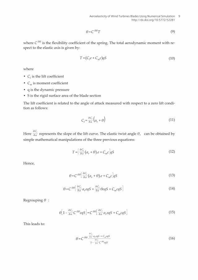
As previously mentioned, flutter is caused by the superposition of two structural modes –pitch and plunge. The pitch mode is described by a rotational movement around the elasticcentre of the airfoil whereas the plunge mode is a vertical up and down motion at the bladetip. Theodorsen [16-18] developed a method to analyze aeroelastic stability. The technique isdescribed by equations (61) and (62). α is the angle of attack (AoA), α0 is the static AoA, C(k)is the Theodorsen complex valued function, h the plunge height, L is the lift vector posi‐tioned at 0.25 of the chord length, M is the pitching moment about the elastic axis, U is thefree velocity, ω is the angular velocity and a, b, d1 and d2 are geometrical quantities asshown in Figure 11.
Figure 11. Model defining parameters
Aeroelasticity of Wind Turbines Blades Using Numerical Simulationhttp://dx.doi.org/10.5772/52281
11

L =2πρU 2b{ iωC (k )h 0
U + C(k )α0 + 1 + C(k )(1 - 2a)iωbα0
2U -ω 2bh 0
2U 2 +ω 2b 2aα0
2U 2 } (25)
M =2πρU 2b{d1iωC (k )h 0
U + C(k )α0 + 1 + C(k )(1 - 2a)iωbα02U + d2
iωbα02U - ω 2b 2a
2U 2 h 0 + ( 18 + a 2) ω 2b 3∝0
2U 2 } (26)
Theodorsen’s equation can be rewritten in a form that can be used and analyzed in MatlabSimulink as follows:
L =2πρU 2b{ C (k )U h + C(k )∝ + 1 + C(k )(1 - 2a) b
2U ∝ + b2U 2 h - b 2a
2U 2 ∝ } (27)
M =2πρU 2b{d1C (k )h .
U + C(k )∝ + 1 + C(k )(1 - 2a) b2U ∝ k + d2
b2U ∝ + ab2
2U 2 h - ( 18 + a 2) b 3∝
2U 2 } (28)
3.3.1. Flutter movement
The occurrence of the flutter has been illustrated in Section 2 (Figure 3). To better under‐stand this complex phenomenon, we describe flutter as follows: aerodynamic forces excitethe mass – spring system illustrated in Figure 12. The plunge spring represents the flexionrigidity of the structure whereas the rotation spring represents the rotation rigidity.
Figure 12. Illustration of both pitch and plunge
3.3.2. Flutter equations
The flutter equations originate in the relation between the generalized coordinates and theangle of attack of the model that can be written as:
α(x, y, t)=θT + θ(t) + h (t )U 0
+ l (x)θ (t )˙U 0
-wg (x , y , t )
U 0(29)
The Lagrangian form equations are constructed for the mechanical system. The first one cor‐responds to the vertical displacement z and the other is for the angle of attack α :
Advances in Wind Power12

J0α + mdcos(α)z + c(α - α0)=M0 (30)
mz + mdcos(α)α - msin(α)α 2˙ + kz = FZ (31)
Numerical solution of these equations requires expressing Fz and Mo as polynomials of α.
Moreover, Fz(α)= 12 ρSV 2Cz(α) and Mo(α)= 1
2 ρLSV 2Cm0(α) for S being the surface of theblade, Cz, the lift coefficient, Cm0 being the pitch coefficient, Fz being the lift, Mo, the pitchmoment. Cz and Cm values are extracted from NACA 4412 data. Third degree interpolationsfor Cz and Cm with respect to the AoA are given below:
Cz = - 0.0000983 α 3 - 0.0003562α 2 + 0.1312α + 0.4162
Cm0 = - 0.00006375α 3 + 0.00149α 2 - 0.001185 α - 0.9312
These equations will be used in the modeling of a lumped representation of flutter present‐ed in the last section of this chapter.
4. Computational fluid dynamics (CFD) methods in aeroelastic modeling
Aeroelastic modeling of wind blades require complex representation of both fluid flows, in‐cluding turbulence, and structural response. Fluid mechanics aims at modeling fluid flowand its effects. When the geometry gets complex (flow becomes unsteady with turbulenceintensity increasing), it is impossible to solve analytically the flow equations. With the ad‐vent of high efficiency computers, and improvement in numerical techniques, computation‐al fluid dynamics (CFD), which is the use of numerical techniques on a computer to resolvetransport, momentum and energy equations of a fluid flow has become more and more pop‐ular and the accuracy of the technique has been an a constant upgrading trend. Aeroelasticmodeling of wind blades includes fluid-structure interaction and is, in fact, a science whichstudies the interaction between elastic, inertial and aerodynamic forces. The aeroelastic anal‐ysis is based on modeling using ANSYS and CFX software. CFX uses a finite volume meth‐od to calculate the aerodynamic solicitations which are transmitted to the structural moduleof ANSYS. Within CFX, several parameters need to be defined such as the turbulence model,the reduced frequency, the solver type, etc. and the assumptions and limitations of eachmodel need to be well understood in order to validate the quality and pertinence of any aer‐oelastic model. These calibration considerations will be illustrated in the stall modeling sec‐tion as an example.
4.1. Dynamic stall
In this section of the chapter, we will illustrate aeroelastic modeling of dynamic stall on aS809 airfoil for a wind blade. The aim of this section, apart from illustrating this aeroelasticphenomenon is to emphasize on the need of parameter calibration (domain size, mesh size,
Aeroelasticity of Wind Turbines Blades Using Numerical Simulationhttp://dx.doi.org/10.5772/52281
13
turbulence and transition model) in CFD analysis.The different behaviour of lift as the AoAincreases or decreases leads to significant hysteresis in the air loads and reduced aerody‐namic damping, particularly in torsion. This can cause torsional aeroelastic instabilities onthe blades. Therefore, the consideration of dynamic stall is important to predict the unsteadyblade loads and, also, to define the operational boundaries of a wind turbine. In all the fol‐lowing examples, the CFD based aeroelastic models are run on the commercial ANSYS-CFXsoftware. CFX, the fluid module of the software, models all the aerodynamic parameters ofthe wind flow. ANSYS structural module defines all the inertial and structural parameters ofthe airfoil and calculates the response and stresses on the structure according to given solici‐tations. The MFX module allows fluid-structure modelling, i.e., the results of the aerody‐namic model are imported as solicitations in the structural module. The continuousexchange of information allows a multi-physics model that, at all time, computes the actionof the fluid on the structure and the corresponding impact of the airfoil motion on the fluidflow.
4.1.1. Model and convergence studies
4.1.1.1. Model and experimental results
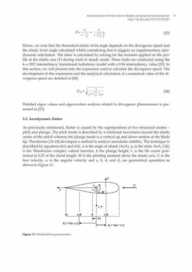
In an attempt to calibrate the domain size, mesh size, turbulence model and transition mod‐el, an S809 profile, designed by NREL, was used.
Figure 13. S809 airfoil
This airfoil has been chosen as experimental results and results from other sources are avail‐able for comparison. The experimental results have been obtained at the Low Speed Labora‐tory of the Delft University [31] and at the Aeronautical and Astronautical ResearchLaboratory of the Ohio State University [32]. The first work [31], performed by Somers, useda 0.6 meters chord model at Reynolds numbers of 1 to 3 million and provides the character‐istics of the S809 profile for angles of incidence from -200 to 200. The second study [32], real‐ized by Ramsey, gives the characteristics of the airfoil for angles of incidence ranging from-200 to 400. The experiments were conducted on a 0.457 meters chord lenght for Reynoldsnumbers of 0.75 to 1.5 million. Moreover, this study provides experimental results for thestudy of the dynamic stall for incidence angles of (80, 140 and 200) oscillating at (±5.50 and ±100) at different frequencies for Reynolds numbers between 0.75 and 1.4 million.
Advances in Wind Power14

4.1.1.2. Convergence studies
In this section, we will focus on the definition of a calculation domain and an adapted meshfor the flow modelling around the mentioned airfoil. This research is realized by the studyof the influence of the distance between the boundaries and the airfoil, the influence of thesize of the chord for the same Reynolds number and finally, the influence of the number ofelements in the mesh and computational time.
4.1.1.3. Computational domain
The computational domain is defined by a semi-disc of radius I1×c around the airfoil and tworectangles in the wake, of length I2×c. This was inspired from works conducted by Bhaskaranpresented in Fluent tutorial. As the objective of this study was to observe how the distance be‐tween the domain boundary and the airfoil affects the results, only I1 and I2 were varied withother values constant. As these two parameters will vary, the number of elements will also vary.To define the optimum calculation domain, we created different domains linked to a prelimina‐ry arbitrary one by a homothetic transformation with respect to the centre G and a factor b. Fig‐ure 14 gives us an idea of the different parameters and the outline of the computational domainwhereas table 1 presents a comparison of the different meshed domains.
Figure 14. Shape of the calculation domain
Figure 15 below respectively illustrates the drag and lift coefficients as a function of the ho‐mothetic factor b for different angles of attack.
Table 1. Description of the trials through homothetic transformation
Aeroelasticity of Wind Turbines Blades Using Numerical Simulationhttp://dx.doi.org/10.5772/52281
15

Figure 15. Drag and lift coefficients vs. homothetic factor for different angles of attack
The drag coefficient diminishes as the homothetic factor increases but tends to stabilize. Thisstabilization is faster for low angles of attack (AoA) and seems to be delayed for larger ho‐mothetic factors and increasing AoA. The trend for the lift coefficients as a function of thehomothetic factor is quite similar for the different angles of attack except for an angle of 8.20.The evolution of the coefficients towards stabilization illustrate an important physical phe‐nomenon: the further are the boundary limits from the airfoil, this allows more space for theturbulence in the wake to damp before reaching the boundary conditions imposed on theboundaries. Finally, a domain having a radius of semi disc 5.7125 m, length of rectangle9,597 m and width 4.799 m was used.
4.1.1.4. Meshing
Unstructured meshes were used and were realized using the CFX-Mesh. These meshes aredefined by the different values in table 2. We kept the previously mentioned domain.
Table 2. Mesh parameters
Figure 16 gives us an appreciation of the mesh we have used of in our simulations:
Figure 16. Unstructured mesh along airfoil, boundary layer at leading edge and boundary layer at trailing edge
Advances in Wind Power16

Several trials were performed with different values of the parameters describing the mesh inorder to have the best possible mesh. Lift and drag coefficient distributions have been com‐puted according to different AoA for a given Reynolds number and the results were com‐pared with experiments. The mesh option that provided results which fitted the best withthe experimental results was used. The final parameters of the mesh were 66772 nodes and48016 elements.
4.1.1.5. Turbulence model calibration
CFX proposes several turbulence models for resolution of flow over airfoils. Scientific litera‐ture makes it clear that different turbulence models perform differently in different applica‐tions. CFX documentation recommends the use of one of three models for such kind ofapplications, namely the k-ω model, the k-ω BSL model and the k-ω SST model. The Wilcoxk-ω model is reputed to be more accurate than k-ε model near wall layers. It has been suc‐cessfully used for flows with moderate adverse pressure gradients, but does not succeedwell for separated flows. The k-ω BSL model (Baseline) combines the advantages of the Wil‐cox k-ω model and the k-ε model but does not correctly predict the separation flow forsmooth surfaces. The k-ω SST model accounts for the transport of the turbulent shear stressand overcomes the problems of k-ω BSL model. To evaluate the best turbulence model forour simulations, steady flow analyses at Reynolds number of 1 million were conducted onthe S809 airfoil using the defined domain and mesh. The different values of lift and drag ob‐tained with the different models were compared with the experimental OSU and DUT re‐sults. D’Hamonville et al. [24] presents these comparisons which lead us to the followingconclusions: the k-ω SST model is the only one to have a relatively good prediction of thelarge separated flows for high angles of attack. So, the transport of the turbulent shear stressreally improves the simulation results. The consideration of the transport of the turbulentshear stress is the main asset of the k-ω SST model. However, probably a laminar-turbulenttransition added to the model will help it to better predict the lift coefficient between 6° and10°, and to have a better prediction of the pressure coefficient along the airfoil for 20°. Thisassumption will be studied in the next section where the relative performance of adding aparticular transitional model is studied.
4.1.1.6. Transition model
ANSYS-CFX proposes in the advanced turbulence control options several transitional mod‐els namely: the fully turbulent k-ω SST model, the k-ω SST intermittency model, the gammatheta model and the gamma model. As the gamma theta model uses two parameters to de‐fine the onset of turbulence, referring to [33], we have only assessed the relative perform‐ance of the first three transitional models. The optimum value of the intermittencyparameter was evaluated. A transient flow analysis was conducted on the S809 airfoil for thesame Reynolds number at different AoA and using three different values of the intermitten‐cy parameter: 0.92, 0.94 and 0.96. Figure 17 illustrates the drag and lift coefficients obtainedfor these different models at different AoA as compared to DUT and OSU experimental da‐ta. We note that for the drag coefficient, the computed results are quite similar and only dif‐
Aeroelasticity of Wind Turbines Blades Using Numerical Simulationhttp://dx.doi.org/10.5772/52281
17

fer in transient mode exhibiting different oscillations. For large intermittency values, theoscillations are larger. Figure 18 shows that for the lift coefficients, the results from CFX dif‐fer from 8.20. For the linear growth zone, the different results are close to each other. Thedifference starts to appear near maximum lift. The k-ω SST intermittency model with γ=0.92,under predicts the lift coefficients as compared with the experimental results. The resultswith γ=0.94 predicts virtually identical results as compared to the OSU results. The modelwith γ= 0.96 predicts results that are sandwiched between the two experimental ones. Anal‐ysis of the two figures brings us to the conclusion that the model with γ=0.94 provides re‐sults very close to the DUT results. Therefore, we will compare the intermittency modelwith γ=0.94 with the other transitional models.
Figure 17. Drag and lift coefficients for different AoA using different intermittency values
Figure 18 illustrates the drag and lift coefficients for different AoA using different transition‐al models.
Figure 18. Drag and lift coefficients for different AoA using different transitional models
Figure 18 shows that the drag coefficients for the three models are very close until 180 afterwhich the results become clearly distinguishable. As from 200, the γ-θ model over predictsthe experimental values whereas such phenomena appear only after 22.10 for the two othermodels. For the lift coefficients, Figure 18 shows that the k-ω SST intermittency models pro‐vide results closest to the experimental values for angles smaller than 140. The k-ω SST mod‐el under predicts the lift coefficients for angles ranging from 60 to 140. For angles exceeding200, the intermittency model does not provide good results. Hence, we conclude that thetransitional model helps in obtaining better results for AoA smaller than 140. However, forAoA greater than 200, a purely turbulent model needs to be used.
Advances in Wind Power18
4.1.2. Results
In order to validate the quality of stall results, the latter are compared with OSU experimen‐tal values and with Leishman-Beddoes model. Moreover, modelling of aeroelastic phenom‐ena is computationally very demanding such that we have opted for an oscillation of 5.50
around 80, 140 and 200 for a reduced frequency of k= ωc2U∞
=0.026 , where c is the length of thechord of the airfoil and U∞ is the unperturbed flow velocity. From a structural point of view,the 0.457 m length profile will be submitted to an oscillation about an axis located at 25% ofthe chord. The results which follow illustrates the quality of our aeroelastic stall modellingat three different angles, all with a variation of 5.5 sin(w)*t.
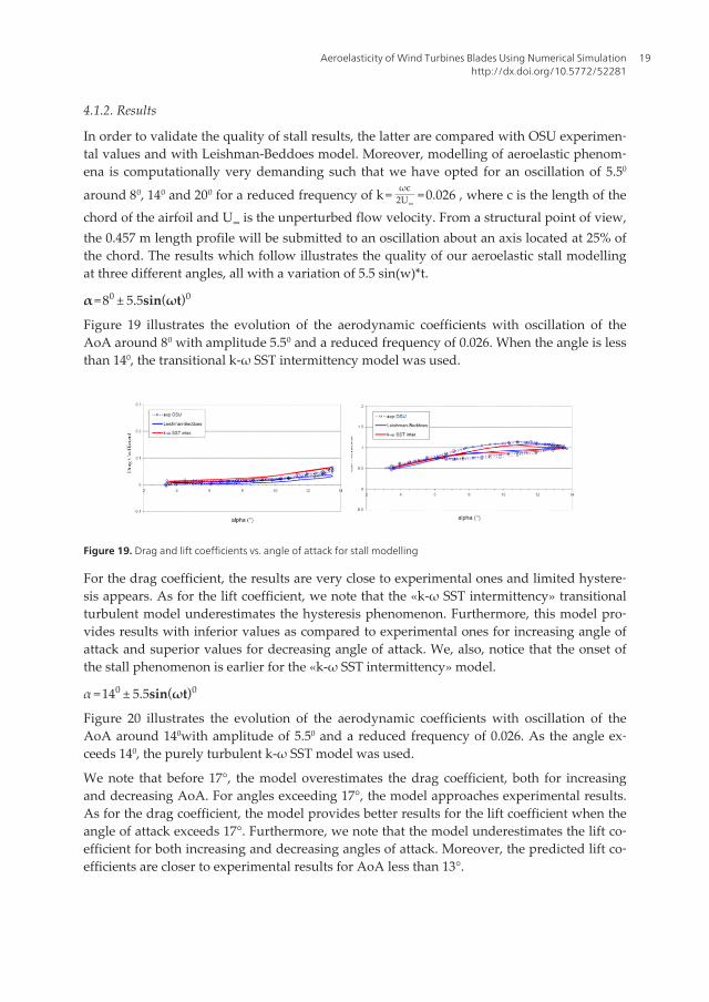
α=80 ± 5.5sin(ωt)0
Figure 19 illustrates the evolution of the aerodynamic coefficients with oscillation of theAoA around 80 with amplitude 5.50 and a reduced frequency of 0.026. When the angle is lessthan 140, the transitional k-ω SST intermittency model was used.
Figure 19. Drag and lift coefficients vs. angle of attack for stall modelling
For the drag coefficient, the results are very close to experimental ones and limited hystere‐sis appears. As for the lift coefficient, we note that the «k-ω SST intermittency» transitionalturbulent model underestimates the hysteresis phenomenon. Furthermore, this model pro‐vides results with inferior values as compared to experimental ones for increasing angle ofattack and superior values for decreasing angle of attack. We, also, notice that the onset ofthe stall phenomenon is earlier for the «k-ω SST intermittency» model.
α =140 ± 5.5sin(ωt)0
Figure 20 illustrates the evolution of the aerodynamic coefficients with oscillation of theAoA around 140with amplitude of 5.50 and a reduced frequency of 0.026. As the angle ex‐ceeds 140, the purely turbulent k-ω SST model was used.
We note that before 17°, the model overestimates the drag coefficient, both for increasingand decreasing AoA. For angles exceeding 17°, the model approaches experimental results.As for the drag coefficient, the model provides better results for the lift coefficient when theangle of attack exceeds 17°. Furthermore, we note that the model underestimates the lift co‐efficient for both increasing and decreasing angles of attack. Moreover, the predicted lift co‐efficients are closer to experimental results for AoA less than 13°.
Aeroelasticity of Wind Turbines Blades Using Numerical Simulationhttp://dx.doi.org/10.5772/52281
19
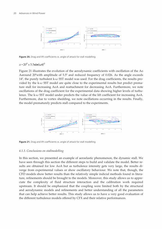
Figure 20. Drag and lift coefficients vs. angle of attack for stall modelling
α =200 ± 5.5sin(ωt)0
Figure 21 illustrates the evolution of the aerodynamic coefficients with oscillation of the AoAaround 200with amplitude of 5.50 and reduced frequency of 0.026. As the angle exceeds140, the purely turbulent k-ω SST model was used. For the drag coefficients, the results pro‐vided by the k-ω SST model are quite close to the experimental results but predict prema‐ture stall for increasing AoA and reattachment for decreasing AoA. Furthermore, we noteoscillations of the drag coefficient for the experimental data showing higher levels of turbu‐lence. The k-ω SST model under predicts the value of the lift coefficient for increasing AoA.Furthermore, due to vortex shedding, we note oscillations occurring in the results. Finally,the model prematurely predicts stall compared to the experiments.
Figure 21. Drag and lift coefficients vs. angle of attack for stall modelling
4.1.3. Conclusions on stallmodelling
In this section, we presented an example of aeroelastic phenomenon, the dynamic stall. Wehave seen through this section the different steps to build and validate the model. Better re‐sults are obtained for low AoA but as turbulence intensity gets very large, the results di‐verge from experimental values or show oscillatory behaviour. We note that, though, theCFD models show better results than the relatively simple indicial methods found in litera‐ture, refinements should be brought to the models. Moreover, this study allows us to appre‐ciate the complexity of fluid structure interaction and the calibration work requiredupstream. It should be emphasized that the coupling were limited both by the structuraland aerodynamic models and refinements and better understanding of all the parametersthat can help achieve better results. This study allows us to have a very good evaluation ofthe different turbulence models offered by CFX and their relative performances.
Advances in Wind Power20

4.2. Aerodynamic divergence
In this section we will illustrate the different steps in modeling another aeroelastic phenom‐enon, the divergence and whilst using this example to lay emphasis on the ability of CFX-ANSYS software to solve fluid-structure interaction problems. As from the 1980s, nationaland international standards concerning wind turbine design have been enforced. With therefinement and growth of the state of knowledge the “Regulation for the Certification ofWind Energy Conversion Systems” was published in 1993 and further amended and refinedin 1994 and 1998. Other standards aiming at improving security for wind turbines have beenpublished over the years. To abide to such standards, modelling of the aeroelastic phenom‐ena is important to correctly calibrate the damping parameters and the operation conditions.For instance, Nweland [34] makes a proper and complete analysis of the critical divergencevelocity and frequencies. These studies allow operating the machines in secure zones andavoid divergence to occur. Such studies’ importance is not only restrained to divergence butalso apply to other general dynamic response cases of wind turbines. Wind fluctuations atfrequencies close to the first flapwise mode blade natural frequency excite resonant bladeoscillations and result in additional, inertial loadings over and above the quasi-static loadsthat would be experienced by a completely rigid blade. Knowledge of the domain of suchfrequencies allows us to correctly design and operate the machines within IEC and othernorms. We here present a case where stall can be avoided by proper knowledge of its pa‐rameters and imposing specific damping. As the oscillations result from fluctuations of thewind speed about the mean value, the standard deviation of resonant tip displacement canbe expressed in terms of the wind turbulence intensity and the normalized power spectraldensity at the resonant frequency, Ru(n1) [34]:
σx1
x1
- =σu
U-
π
2δRu(n1) Ksx(n1) (32)
where:
Ru(n1)= n.Su(n1)
σ 2u
(33)
•x1
- is the first mode component of the steady tip displacement.
•U-
is the mean velocity (usually averaged over 10 minutes)
• δ is the logarithmic decrement damping
• Ksx(n1) is the size of the reduction factor which is present due to lack of correlation ofwind along the blade at the relevant frequency.
Aeroelasticity of Wind Turbines Blades Using Numerical Simulationhttp://dx.doi.org/10.5772/52281
21

It is clear from equation (32) that a key determinant of resonant tip response is the value ofdamping present. If we consider for instance a vibrating blade flat in the wind, the fluctuat‐ing aerodynamic force acting on it per unit length is given by:
12 ρ(U- - x)2
Cd - C(r) - 12 ρU
- 2
Cd .C(r)≅ρU-
xCdC(r) (34)
where x is the blade flatwise velocity, Cd is the drag coefficient and C(r) is the local blade
chord. Hence the aerodynamic damping per unit length, Ca^ (r)=ρU
-CdC(r) and the first aero‐
dynamic damping mode is:
εa1 =Ca1
2m1ω1=∫0
RCa^ (r )μ1
2(r )dr2m1ω1
=ρU
-Cd ∫0
RC (r )μ12(r )dr
2m1ω1
(35)
μ1(r) is the first mode shape and m1 is the generalized mass given by:
m1 = ∫0Rm(r)μ1
2(r)dr (36)
Here, ω1 is the first mode natural frequency given in radian per second. The logarithmicdecrement is obtained by multiplying the damping ratio by 2 π . To properly estimate oper‐ating conditions and damping parameters, knowledge of the vibration frequencies andshape modes are important. The need to know these limits is again justified by the fact thatwhen maximum lift is theoretically achieved toward maximum power when stall and otheraeroelastic phenomena are also approached.
4.2.1. ANSYS-CFX coupling
To achieve the fluid structure coupling study, we make use of the ANSYS multi-domain(MFX). This module was primarily developed for fluid-structure interaction studies. On oneside, the structural part is solved using ANSYS Multiphysics and on the other side, the fluidpart is solved using CFX. The study needs to be conducted on a 3D geometry. If the geome‐tries used by ANSYS and CFX need to have common surfaces (interfaces), the meshes ofthese surfaces can be different. The ANSYS code acts as the master code and reads all themulti-domain commands. It recuperates the interface meshes of the CFX code, creates themapping and communicates the parameters that control the timescale and coupling loops tothe CFX code. The ANSYS generated mapping interpolates the solicitations between the dif‐ferent meshes on each side of the coupling. Each solver realizes a sequence of multi-domain,time marching and coupling iterations between each time steps. For each iteration, eachsolver recuperates its required solicitation from the other domain and then solves it in thephysical domain. Each element of interface is initially divided into n interpolation faces (IP)where n is the number of nodes on that face. The 3D IP faces are transformed into 2D poly‐
Advances in Wind Power22

gons. We, then, create the intersection between these polygons, on one hand, the solver dif‐fusing solicitations and on the other hand, the solver receiving the solicitations. Thisintersection creates a large number of surfaces called control surfaces as illustrated in Figure22. These surfaces are used in order to transfer the solicitation between the structural andfluid domains.
Figure 22. Transfer Surfaces
The respective MFX simultaneous and sequential resolution schemes are presented in fig‐ure 23.
Figure 23. Simultaneous or sequential resolution of CFX and ANSYS
We can make use of different types of resolutions, either using a simultaneous scheme orusing a sequential scheme, in which case we need to choose which domain to solve first. Forlightly coupled domains, CFX literature recommends the use of the simultaneous scheme.As for our case, the domains are strongly coupled and for such reasons, we make use of thesequential scheme. This scheme has as advantage to ensure that the most recent result or so‐licitation of a domain solver is applied to the other solver. In most simulations; the physicsof one domain imposes the requirements of the other domain. Hence, it is essential to ade‐
Aeroelasticity of Wind Turbines Blades Using Numerical Simulationhttp://dx.doi.org/10.5772/52281
23
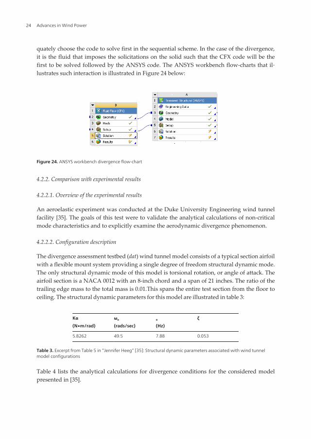
quately choose the code to solve first in the sequential scheme. In the case of the divergence,it is the fluid that imposes the solicitations on the solid such that the CFX code will be thefirst to be solved followed by the ANSYS code. The ANSYS workbench flow-charts that il‐lustrates such interaction is illustrated in Figure 24 below:
Figure 24. ANSYS workbench divergence flow-chart
4.2.2. Comparison with experimental results
4.2.2.1. Overview of the experimental results
An aeroelastic experiment was conducted at the Duke University Engineering wind tunnelfacility [35]. The goals of this test were to validate the analytical calculations of non-criticalmode characteristics and to explicitly examine the aerodynamic divergence phenomenon.
4.2.2.2. Configuration description
The divergence assessment testbed (dat) wind tunnel model consists of a typical section airfoilwith a flexible mount system providing a single degree of freedom structural dynamic mode.The only structural dynamic mode of this model is torsional rotation, or angle of attack. Theairfoil section is a NACA 0012 with an 8-inch chord and a span of 21 inches. The ratio of thetrailing edge mass to the total mass is 0.01.This spans the entire test section from the floor toceiling. The structural dynamic parameters for this model are illustrated in table 3:
Kα
(N∙m/rad)
ωα
(rads/sec)
�α
(Hz)
ζ
5.8262 49.5 7.88 0.053
Table 3. Excerpt from Table 5 in “Jennifer Heeg” [35]: Structural dynamic parameters associated with wind tunnelmodel configurations
Table 4 lists the analytical calculations for divergence conditions for the considered modelpresented in [35].
Advances in Wind Power24

Velocity Dynamic Pressure
(in/sec) (mph) (m/s) (psf) (N/m2)
754 42.8 19.15 4.6 222
Table 4. Analytical calculations for divergence conditions for the considered model presented
However, some parameters were unavailable in [35] such that an iterative design processwas used to build the model in ANSYS. Using parameters specified in [35], a preliminarymodel was built and its natural frequencies verified using ANSYS. The model was succes‐sively modified until a model as close as possible to the model in the experiment was ob‐tained.The aims of the studies conducted in [35] were to: 1) find the divergence dynamicpressure;2)examine the modal characteristics of non-critical modes, both sub-critically andat the divergence condition; 3) examine the eigenvector behaviour. Heeg[35] obtained sever‐al interesting results among which the following graphic showing the variation of the angleof attack with time. The aim of our simulations was to determine how the numerical AN‐SYS-CFX model will compare with experiments.
Figure 25. Divergence of wind tunnel model configuration #2
The test was conducted by setting as close as possible to zero the rigid angle of attack, α0, fora zero airspeed. The divergence dynamic pressure was determined by gradually increasingthe velocity and measuring the system response until it became unstable. The dynamic pres‐sure was being slowly increased until the angle of attack increased dramatically and sud‐denly. This was declared as the divergence dynamic pressure, 5.1 psf (244 N/m2). The timehistory shows that the model oscillates around a new angle of attack position, which is notat the hard stop of the spring. It is speculated that the airfoil has reached an angle of attackwhere flow has separated and stall has occurred [35].
4.2.2.3. The ANSYS-CFX model
The model used in the experiment was simulated using a reduced span-wise numerical do‐main (quasi 2D). The span of the airfoil was reduced 262.5 times, from 21 inches to 0.08 in‐ches or 2.032 mm, while the chord of the airfoil was maintained at 8 inch or 203.2 mm. Weused a cylinder to simulate the torsion spring used in the experiment.
Aeroelasticity of Wind Turbines Blades Using Numerical Simulationhttp://dx.doi.org/10.5772/52281
25

Figure 26. ANSYS built geometry with meshing
4.2.2.4. Results
In [23], the authors have derived the analytical mathematical equation to calculate the diver‐gence velocity, U D . The expression was:
U D = 1
C θθ∂ Cl∂ α e
12 ρS
(37)
In order to calculate the theoretical value of the divergence velocity, certain parameters need tobe found first. These are C θθ, which is specific to the modeled spring, S being inherent to theprofile, e, which depends both on the profile (elastic axis) and on the aerodynamic model, ρ,
which is dependent upon the used fluid and ∂Cl
∂α which depends both on the shape of the pro‐file but, also, on the turbulent model [23]. We note that, as divergence velocity is approached,the elastic twist angle will increase in a very significant manner and tend to infinity [24]. How‐ever, numerical values are finite and cannot model infinite parameters. We will, therefore, for‐mulate the value of the analytical elastic twist angle in order to compare it with the value foundby the coupling. In the case wherein the elastic twist angle introduces no further aerodynamicsolicitations, by introducing α =αr , and resolving for the elastic twist angle, we have:
θr =C θθT = C θθ( ∂Cl
∂α e αr + Cmc)qS (38)
Algebraic manipulations of the expressions lead us to the following formulation:
θ =θr
1 -∂ Cl∂ α C θθeqS
(39)
This leads to:
θ =θr
1 -q
qD
= θr
1 - ( UU D )2 (40)
Advances in Wind Power26

Hence, we can note that the theoretical elastic twist angle depends on the divergencespeed and the elastic twist angle calculated whilst considering that it triggers no supple‐mentary aerodynamic solicitation. To calculate the latter, we will solve for the momentapplied on the profile at the elastic axis (T) during trials in steady mode. These trials areconducted using the k-ω SST intermittency transitional turbulence model with a 0.94 in‐termittency value [24]. To model the flexibility coefficient of the rotational spring C θθ ,used in the NASA experiments we used a cylinder as a torsion spring. The constant ofthe spring used in the experiment is Kα = 5.8262 N∙m/rad and since we used a reducedmodel, with an span 262.5 times smaller than the original, the dimensions and propertiesof the cylinder are such that:
Kαr = 5.8262262.5 N ∙ m
rad = 0.022195 N∙ m / rad (41)
and the flexibility coefficient is:
C θθ = 1Kαr
=45.0552 rad / N ∙m (42)
The slope of the lift ∂Cl
∂α , can be calculated for an angle α =50 in the following way:
∂Cl
∂α =C
l ,α>50 - Cl ,α<50
α > 50 - α < 50(43)
We have calculated the lift coefficient at 4.00 and 6.00 such that:
Cl ,α=4.00 =0.475
and Cl ,α=6.00 =0.703
Hence the gradient can be expressed and calculated as follows:
∂Cl
∂α = 0.703 - 0.4756.0 - 4.0 =0.114 deg -1 =6.532 rad -1
The distance e, between the elastic axis and the aerodynamic centre for the model is 0.375∙b.The rigid area is calculated to be S, being the product of the chord and the span and is calcu‐lated as follows:
S =0.2032•0.5334=0.0004129024m 2
Hence the divergence velocity is calculated as:
U D = 1
C θθ∂ Cl∂ α
ρ2 eS
= 18.78 m / s (44)
Aeroelasticity of Wind Turbines Blades Using Numerical Simulationhttp://dx.doi.org/10.5772/52281
27

The theoretical divergence speed given in Table 4 of the NASA experiment [35] is 19.15 m/s.
This slight difference is due to the value of slope of the lift profile ∂Cl
∂α taken into considera‐tion, which in the NASA work was 2π, or 6.283 rad-1, whereas we used a value of 6.532rad-1 . Furthermore, a difference between our calculated speed and that presented in [35]might also be explained by the size of the used tunnel and the possible wall turbulence in‐teraction. Furthermore, using the model, domain and mesh parameters detailed in the previ‐ous sections of this article, divergence was modelled as follows: the airfoil used in [35] wasfixed and exempted from all rotational degrees of liberty and subjected to a constant flow ofvelocity 15 m s -1 . Suddenly, the fixing is removed and the constant flow can be then com‐pared to a shock wave on the profile. The profile then oscillates with damped amplitude dueto the aerodynamic damping imposed. Figure 27 illustrates the response portrayed by AN‐SYS-CFX software. We can extract the amplitude and frequency of oscillation of around 8Hz which is close to the 7.9 Hz frequency presented in [35].
Figure 27. Oscillatory response to sudden subject to a constant flow of 15m/s
4.3. Aerodynamic flutter
In this section, we illustrate a CFD approach of modeling the most complex and the mostdangerous type of aeroelastic phenomenon to which wind turbine blades are subjected.While illustrating stall phenomenon, we calibrated the CFD parameters for aeroelastic mod‐eling. In the divergence section, the example was used to reinforce the notion of multiphy‐sics modeling, more precisely, emphasis was laid on fluid structure interaction modelingwithin ANSYS-CFX MFX. Flutter example will be used to illustrate the importance of usinglumped method.
4.3.1. Computational requirement and Lumped model
Aeroelastic modeling requires enormous computational capacity. The most recent quad core16 GB processor takes some 216 hours to simulate flutter on a small scale model and that fora 12 second real time frame. The aim of simulating and predicting aeroelastic effects on
Advances in Wind Power28

wind blades has as primary purpose to apply predictive control. However, with such enor‐mous computational time, this is impossible. The need for simplified lumped (2D Matlabbased) models is important. The CFD model is ran preliminarily and the lumped model isbuilt according to simulated scenarios. In this section we will illustrate flutter modeling bothfrom a CFD and lumped method point of view.
4.3.2. Matlab-Simulink and Ansys-CFX tools
For flutter modelling, again, ANSYS-CFX model was used to simulate the complex fluid-structure interaction. However, due to excessively important computational time that ren‐dered the potential of using the predictive results for the application of mitigation controlimpossible, the results of the CFD model was used to build a less time demanding lumpedmodel based on Simulink. Reference [36] describes the Matlab included tool Simulink as anenvironment for multi-domain simulation and Model-Based Design for dynamic and em‐bedded systems. It provides an interactive graphical environment and a customizable set ofblock libraries that let you design, simulate, implement, and test a variety of time-varyingsystems. For the flutter modelling project, the aerospace blockset of Simulink has been used.The Aerospace Toolbox product provides tools like reference standards, environment mod‐els, and aerospace analysis pre-programmed tools as well as aerodynamic coefficient im‐porting options. Among others, the wind library has been used to calculate wind shears andDryden and Von Karman turbulence. The Von Karman Wind Turbulence model uses theVon Karman spectral representation to add turbulence to the aerospace model through pre-established filters. Turbulence is represented in this blockset as a stochastic process definedby velocity spectra. For a blade in an airspeed V, through a frozen turbulence field, with aspatial frequency of Ω radians per meter, the circular speed ω is calculated by multiplying Vby Ω. For the longitudinal speed, the turbulence spectrum is defined as follows:
ψlo =σ 2
ω
V L ω.
0.8( π L ω4b
)0.3
1 + ( 4bωπV
)2(45)
Here, Lω represents the turbulence scale length and σ is the turbulence intensity. The corre‐sponding transfer function used in Simulink is:
ψlo =σu
2π
L vV
(1 + 0.25L vV s)
1 + 1.357L vV s + 0.1987( L v
V s)2s 2
(46)
For the lateral speed, the turbulence spectrum is defined as:
ψla =∓( ω
V)2
1 + ( 3bωπV
)2 .φv(ω) (47)
and the corresponding transfer function can be expressed as :
Aeroelasticity of Wind Turbines Blades Using Numerical Simulationhttp://dx.doi.org/10.5772/52281
29

ψla =∓( s
V)1
1 + ( 3bπV s)1 .Hv(s) (48)
Finally, the vertical turbulence spectrum is expressed as follows:
ψv =∓( ω
V)2
1 + ( 4bωπV
)2 .φω(ω) (49)
and the corresponding transfer function is expressed as follows:
ψv =∓( s
V)1
1 + ( 4bπV s)1 .Hω(s) (50)
The Aerodynamic Forces and Moments block computes the aerodynamic forces and mo‐ments around the center of gravity. The net rotation from body to wind axes is expressed as:
Cω←b =cos (α)cos (β) sin (β) sin (α)cos (β)-cos (α)sin (β) cos (β) -sin (α)sin (β)
-sin (α) 0 cos (α) (51)
On the other hand, the fluid structure interaction to model aerodynamic flutter was madeusing ANSYS multi domain (MFX). As previously mentioned, the drawback of the AN‐SYS model is that it is very time and memory consuming. However, it provides a verygood option to compare and validate simplified model results and understand the intrin‐sic theories of flutter modelling. On one hand, the aerodynamics of the application ismodelled using the fluid module CFX and on the other side, the dynamic structural partis modelled using ANSYS structural module. An iterative exchange of data between thetwo modules to simulate the flutter phenomenon is done using the Workbench interface.
4.3.3. Lumped model results
We will first present the results obtained by modeling AoA for configuration # 2 of reference[35] (also, discussed in the divergence section 4.2) for an initial AoA of 0°. As soon as diver‐gence is triggered, within 1 second the blade oscillates in a very spectacular and dangerousmanner. This happens at a dynamic pressure of 5,59lb/pi2 (268 N/m2). Configuration #2 uses,on the airfoil, 20 elements, unity as the normalized element size and unity as the normalizedairfoil length. Similarly, the number of elements in the wake is 360 and the correspondingnormalized element size is unity and the normalized wake length is equal to 2. The resultsobtained in [35] are illustrated in Figure 28:
Advances in Wind Power30

Figure 28. Flutter response- an excerpt from [23]
We notice that at the beginning there is a non-established instability, followed by a recurrentoscillation. The peak to peak distance corresponds to around 2.5 seconds that is a frequencyof 0.4 Hz. The oscillation can be defined approximately by an amplitude of 00 ± 170. . Thesame modelling was performed using the Simulink model and the result for the AoA varia‐tion and the plunge displacement is shown below:
Figure 29. Flutter response obtained from Matlab Aerospace blockset
We note that for the AoA variation, the aerospace blockset based model provides very similarresults with Heeg’s results [35]. The amplitude is, also, around 00 ± 170 and the frequency is0.45 Hz. Furthermore, we notice that the variation is very similar. We can conclude that theaerospace model does represent the flutter in a proper manner. It is important to note that thisis a special type of flutter. The frequency of the beat is zero and, hence, represents divergence of“zero frequency flutter”. Using Simulink, we will vary the angular velocity of the blade untilthe eigenmode tends to a negative damping coefficient. The damping coefficient, ζ is obtained
as: ζ = c2mω , ω is measured as the Laplace integral in Simulink, c is the viscous damping and ω
= km . Figure 30 illustrates the results obtained for the variation of the damping coefficient
against rotational speed and flutter frequency against rotor speed. We can note that as the rota‐tion speed increases, the damping becomes negative, such that the aerodynamic instabilitywhich contributes to an oscillation of the airfoil is amplified. We also notice that the frequencydiminishes and becomes closer to the natural frequency of the system. This explains the rea‐son for which flutter is usually very similar to resonance as it occurs due to a coalescing of dy‐namic modes close to the natural vibrating mode of the system.
Aeroelasticity of Wind Turbines Blades Using Numerical Simulationhttp://dx.doi.org/10.5772/52281
31

Figure 30. Damping coefficient against rotational speed and flutter frequency against rotor speed
Figure 31. Flutter simulation with ANSYS-CFX at 1) 1.8449 s, 2) 1.88822 s and 1.93154s
We present here the results obtained for the same case study using ANSYS-CFX. The fre‐quency of the movement using Matlab is 6.5 Hz while that using the ANSYS-CFX model is6.325 Hz compared with the experimental value of 7.1Hz [35]. Furthermore, the amplitudesof vibration are very close as well as the trend of the oscillations. For the points identified as1, 2 and 3 on the flutter illustration, we illustrate the relevant flow over the airfoil. The maxi‐mum air speed at moment noted 1 is 26.95 m/s. We note such a velocity difference over theairfoil that an anticlockwise moment will be created which will cause an increase in the an‐gle of attack. Since the velocity, hence, pressure difference, is very large, we note from theflutter curve, that we have an overshoot. The velocity profile at moment 2, i.e., at 1.88822sshows a similar velocity disparity, but of lower intensity. This is visible as a reduction in thegradient of the flutter curve as the moment on the airfoil is reduced. Finally at moment 3, wenote that the velocity profile is, more or less, symmetric over the airfoil such that the mo‐ment is momentarily zero. This corresponds to a maximum stationary point on the flutter
Advances in Wind Power32

curve. After this point, the velocity disparity will change position such that angle of attackwill again increase and the flutter oscillation trend maintained, but in opposite direction.This cyclic condition repeats and intensifies as we have previously proved that the dampingcoefficient tends to a negative value.
Author details
Drishtysingh Ramdenee1,2, Adrian Ilinca1 and Ion Sorin Minea1
1 Wind Energy Research Laboratory, Université du Québec à Rimouski, Rimouski, Canada
2 Institut Technologique de la Maintenance Industrielle, Sept Îles, Canada
References
[1] J. Scheibert et al. " Stress field at a sliding frictional contact: Experiments and calcula‐tions" Journal of the Mechanics and Physics of Solids 57 (2009) 1921–1933
[2] P. Destuynder, Aéroélasticité et Aéroacoustique, 85, 2007
[3] www.nrel.gov/docs/fy06osti/39066.pdf
[4] Gunner et al. Validation of an aeroelastic model of Vestas V39. Risoe Publication, DK180 91486
[5] Gabriel Saiz. Turbomachinery Aeroelasticity using a Time-Linearized Multi-BladeRow Approach. Ph.D thesis Imperial College, London, 2008
[6] Christophe Pierre et al. Localization of Aeroelastic Modes in High Energy Turbines,Journal of Propulsion and Power. Vol 10, June 1994
[7] Ivan McBean et al. Prediction of Flutter of Turbine Blades in a Transonic AnnularCascade. Journal of Fluids Engineering, ASME 2006
[8] Srinivasan. A. V. Flutter and Resonant Vibration Characteristics of Engine Blades,ASME 1997, page 774-775
[9] Liu. F et al. Calibration of Wing Flutter by a Coupled Fluid Structure Method, Jour‐nal of Aeroelasticity, 38121, 2001
[10] K. Rao. V. Kaza. Aeroelastic Response of Metallic & Composite Propfan models inYawned Flow. NASA Technical Memorandum 100964 AIAA-88-3154
[11] C. Wieseman et al. Transonic Small Disturbance and Linear Analyses for the ActiveAeroelastic Wing Program
Aeroelasticity of Wind Turbines Blades Using Numerical Simulationhttp://dx.doi.org/10.5772/52281
33

[12] Todd O’Neil. Non Linear Aeroelastic Response Analyses and ExperimentsAIAA-1996
[13] R. Bisplinghoff, H. Ashley, R. Halfman, « Aeroelasticity »Dover Editions, 1996
[14] Bisplinghoff R.L.Aeroelasticity. Dover Publications: New York, 1955
[15] Fung, Y.C., 1993. An Introduction to the Theory of Aeroelasticity. Dover PublicationsInc., New York
[16] Leishman, J.G., 2000. Principles of Helicopter Aerodynamics. Cambridge UniversityPress, Cambridge
[17] J.W. Larsen et al. / Journal of Fluids and Structures 23 (2007) 959–982
[18] VISCWIND, 1999. Viscous effects on wind turbine blades, final report on the JOR3CT95-0007, Joule III project, Technical Report, ET-AFM-9902, Technical University ofDenmark
[19] D.Ramdenee et A.Ilinca « An insight to Aeroelastic Modelling » Internal Report,UQAR, 2011
[20] Spalart PR and Allmaras SR ‘’One equation turbulence model for aerodynamicflows’’Jan 1993
[21] Davison and Rizzi A’’Navier Stokes computation of Airfoil in Stall algebraic stressesmodel, Jan 1992’’
[22] Eppler R airfoil design and data, NY springs Veng 1990. R. Michel et al. ‘’Stabilitycalculations and transition criteria on 2D and 3D flows’’ Laminar and turbulent No‐vosibirski, USSR,1984
[23] D. Ramdenee, A. Ilinca. An insight into computational fluid dynamics.Rapport Tech‐nique, UQAR/LREE
[24] T. Tardif d’Hamonville, A. Ilinca Modélisation et Analyse des Phénomènes Aéroélas‐tiques pour une pale d’Éolienne Masters Thesis, UQAR/LREE
[25] T. Tardif d’Hamonville, A. Ilinca. Modélisation de l’écoulement d’air autour d’unproil de pale d’éolienne,Phase 1: Domaine étude et Maillage. Rapport Technique,UQAR/LREE-05, Décembre 2008
[26] Raymond L.Bisphlinghoff, Holt Ashley and Robert L.Halfman, Aeroelasticity, Dover1988
[27] www.ltas.mct.ulg.ac.be/who/stainier/docs/aeroelastcite.pdf
[28] Theodorsen, T., General theory of aerodynamic instability and the mechanism of flut‐ter, NACA Report 496, 1935.
[29] Fung, Y. C., An Introduction to the Theory of Aeroelasticity. Dover Publications Inc.:New York, 1969; 210-216
Advances in Wind Power34

[30] Dowell, E. E. (Editor), A Modern Course in Aeroelasticity. Kluwer Academic Pub‐lishers: Dordrecht, 1995; 217-227
[31] Somers, D.M. “Design and Experimental Results for the S809 Airfoil”. NREL/SR-440-6918, 1997
[32] Reuss Ramsay R., Hoffman M. J., Gregorek G. M. “Effects of Grit Roughness andPitch Oscillations on the S809 Airfoil.” Master thesis, NREL Ohio State University,Ohio, NREL/TP-442-7817, December 1995.
[33] ANSYS CFX, Release 11.0
[34] Nweland, D.E (1984) Random Vibrations and Spectral Analysis, Longman, UK
[35] Jennifer Heeg, “Dynamic Investigation of Static Divergence: Analysis and Testing”,Langley Research Center, Hampton, Virginia, National Aeronautics and Space Ad‐ministration
[36] Matlab-Simulink documentations. Release 8b
Aeroelasticity of Wind Turbines Blades Using Numerical Simulationhttp://dx.doi.org/10.5772/52281
35