Aerodynamic Drag Reduction Technologies Testing of … · aerodynamic devices on select vocational vehicles and trailers, as accurately as possible given limited test time and budget

NREL is a national laboratory of the U.S. Department of Energy Office of Energy Efficiency & Renewable Energy Operated by the Alliance for Sustainable Energy, LLC

This report is available at no cost from the National Renewable Energy Laboratory (NREL) at www.nrel.gov/publications.

Contract No. DE-AC36-08GO28308

Aerodynamic Drag Reduction Technologies Testing of Heavy-Duty Vocational Vehicles and a Dry Van Trailer Adam Ragatz and Matthew Thornton National Renewable Energy Laboratory

Produced under direction of California Air Resources Board (CARB) by the National Renewable Energy Laboratory (NREL) under Work for Others Agreement number FIA-11-1763 and Task No WW4A.1007.

Technical Report NREL/TP-5400-64610 October 2016

NREL is a national laboratory of the U.S. Department of Energy Office of Energy Efficiency & Renewable Energy Operated by the Alliance for Sustainable Energy, LLC

This report is available at no cost from the National Renewable Energy Laboratory (NREL) at www.nrel.gov/publications.

Contract No. DE-AC36-08GO28308

National Renewable Energy Laboratory 15013 Denver West Parkway Golden, CO 80401 303-275-3000 • www.nrel.gov

Aerodynamic Drag Reduction Technologies Testing of Heavy-Duty Vocational Vehicles and a Dry Van Trailer Adam Ragatz and Matthew Thornton National Renewable Energy Laboratory

Prepared under Task No. WW4A.1007

Technical Report NREL/TP-5400-64610 October 2016

NOTICE

This manuscript has been authored by employees of the Alliance for Sustainable Energy, LLC (“Alliance”) under Contract No. DE-AC36-08GO28308 with the U.S. Department of Energy (“DOE”).

This report was prepared as an account of work sponsored by an agency of the United States government. Neither the United States government nor any agency thereof, nor any of their employees, makes any warranty, express or implied, or assumes any legal liability or responsibility for the accuracy, completeness, or usefulness of any information, apparatus, product, or process disclosed, or represents that its use would not infringe privately owned rights. Reference herein to any specific commercial product, process, or service by trade name, trademark, manufacturer, or otherwise does not necessarily constitute or imply its endorsement, recommendation, or favoring by the United States government or any agency thereof. The views and opinions of authors expressed herein do not necessarily state or reflect those of the United States government or any agency thereof.

Cover Photos by Dennis Schroeder: (left to right) NREL 26173, NREL 18302, NREL 19758, NREL 29642, NREL 19795.

NREL prints on paper that contains recycled content.

iii This report is available at no cost from the National Renewable Energy Laboratory (NREL) at www.nrel.gov/publications.

Acknowledgments This work was generously supported by the California Air Resources Board under agreement number 11-600, National Renewable Energy Laboratory contract number FIA-11-1763.

The statements and conclusions in this report are those of the authors and not necessarily those of the California Air Resources Board. The mention of commercial products, their source, or their use in connection with material reported herein is not to be construed as actual or implied endorsement of such products.

iv This report is available at no cost from the National Renewable Energy Laboratory (NREL) at www.nrel.gov/publications.

List of Acronyms AMT automated manual transmission CARB California Air Resources Board DPF diesel particulate filter FTP Federal Test Procedure GPS global positioning system Hz hertz mph miles per hour MSS micro soot sensor NREL National Renewable Energy Laboratory PM particulate matter

v This report is available at no cost from the National Renewable Energy Laboratory (NREL) at www.nrel.gov/publications.

Table of Contents List of Acronyms ........................................................................................................................................ iv List of Figures ............................................................................................................................................ vi List of Tables ............................................................................................................................................. vii Project Background and Objective ........................................................................................................... 1 Project Summary ......................................................................................................................................... 1 Test Vehicles ............................................................................................................................................... 2

Box Trucks ............................................................................................................................................. 2 Tractor-Trailer ........................................................................................................................................ 3

Aerodynamic Devices ................................................................................................................................. 3 Coastdown Testing ..................................................................................................................................... 5 On-Road Testing ....................................................................................................................................... 10 Results and Discussion ............................................................................................................................ 12

Coastdown Testing – Box Trucks and Tractor-Trailer ......................................................................... 12 On-Road Testing – Box Trucks ............................................................................................................ 16

Simulation Results .................................................................................................................................... 21 Conclusion ................................................................................................................................................. 38 Appendix A – Additional Truck Dimensions .......................................................................................... 39

Class 6 Box Truck ................................................................................................................................ 39 Class 4 Box Truck ................................................................................................................................ 41

Appendix B – Additional Tractor-Trailer Dimensions ........................................................................... 43 Appendix C – Heavy-Duty On-Road Vehicle Opacity and Engine Repair Durability ......................... 44

Background .......................................................................................................................................... 44 Instrumentation ..................................................................................................................................... 44 Test Plan ............................................................................................................................................... 45 Results .................................................................................................................................................. 47 Conclusion ............................................................................................................................................ 51

vi This report is available at no cost from the National Renewable Energy Laboratory (NREL) at www.nrel.gov/publications.

List of Figures Figure 1. Box truck vehicles with aerodynamic devices installed. Class 6 (left), Class 4 (right), coastdown

vehicles (top), on-road test and control vehicles (bottom) ....................................................... 4 Figure 2. Class 7 tractor-trailer test vehicle with aerodynamic improvement devices installed ................... 5 Figure 3. Coastdown test track ...................................................................................................................... 6 Figure 4. Coastdown track grade .................................................................................................................. 6 Figure 5. Stationary roadside weather station, Airmar 150WX .................................................................... 7 Figure 6. On-board ultrasonic anemometer, YOUNG model 81000 ............................................................ 8 Figure 7. Raw GPS data from 12 coastdown runs (six in each direction) .................................................... 8 Figure 8. Example of road load force vs. vehicle speed and resulting fit curve ........................................... 9 Figure 9. On-road test section ..................................................................................................................... 11 Figure 10. Secondary fuel weigh tank and scale ......................................................................................... 11 Figure 11. Observed change in CdA and road load without wind correction. ............................................ 15 Figure 12. Observed change in CdA and road load with wind correction. ................................................. 16 Figure 13. On-road fuel consumption test results ....................................................................................... 18 Figure 14. On-road fuel savings from chassis skirts under various wind conditions .................................. 19 Figure 15. California average wind speed .................................................................................................. 20 Figure 16. Theoretical road load components. Aerodynamics are more important for lightly loaded

vehicles................................................................................................................................... 21 Figure 17. Percent change in fuel economy for a 1% change in Cd ........................................................... 22 Figure 18. Simulated drive cycle fuel consumption results ........................................................................ 26 Figure 19. Model tuning – step van ............................................................................................................ 28 Figure 20. Theoretical vs. J1939 daily fuel for step vans ........................................................................... 28 Figure 21. Large box truck simulation results. Probability distribution (left) and cumulative distribution

(right) ..................................................................................................................................... 30 Figure 22. Large box truck simulation results – cumulative distribution of potential greenhouse gas

savings .................................................................................................................................... 30 Figure 23. Simulation results – all models, 5% CdA improvement (left), 10% CdA improvement (right),

probability distributions (top), cumulative distributions (bottom) ......................................... 31 Figure 24. Daily fuel saved – gallons vs. percentage for a 5% CdA improvement .................................... 32 Figure 25. Simulation result for a 5% CdA improvement, cumulative distributions – total gallons (left),

percent savings (right) ............................................................................................................ 33 Figure 26. Kinetic intensity vs. average speed ............................................................................................ 33 Figure 27. Simulation drive cycle trends – fuel savings vs. average speed, kinetic intensity, and engine

speed at 65 mph ...................................................................................................................... 34 Figure 28. U.S. EPA cluster analysis, Cluster 1: low-speed, aggressive (green); Cluster 2: mid-speed

(orange); Cluster 3: high-speed steady (purple); driving days used for this reports analysis (black); biggest fuel savers on a “total gallon” basis (red); biggest fuel savers on a percentage basis (yellow) ....................................................................................................... 35

Figure 29. Vehicle activity and cluster by vocational grouping, all vehicle days considered (black), member of the specified vocation (yellow) ............................................................................ 37

Figure 30. Instrumentation test setup .......................................................................................................... 45 Figure 31. Testing platforms ....................................................................................................................... 46 Figure 32. DPF progressive failure ............................................................................................................. 47 Figure 33. Cummins ISL results. Snap opacity (left) and engine FTP (right) ............................................ 47 Figure 34. Gravimetric filter vs. integrated AVL MSS .............................................................................. 48 Figure 35. FTP vs. opacity fit curves .......................................................................................................... 49 Figure 36. Results – MaxxForce 10 (blue), Cummins ISL (red) ................................................................ 49 Figure 37. FTP instrumentation correlogram .............................................................................................. 50

vii This report is available at no cost from the National Renewable Energy Laboratory (NREL) at www.nrel.gov/publications.

Figure 38. Instrumentation comparison ...................................................................................................... 50 Figure 39. Failure level projections ............................................................................................................ 51

List of Tables Table 1. Vehicle Specifications .................................................................................................................... 2 Table 2. Tractor and Trailer .......................................................................................................................... 3 Table 3. Box Truck Aerodynamic Devices, Weights, and Corresponding Test Vehicle .............................. 4 Table 4. Tractor-Trailer Aerodynamic Devices and Weights ....................................................................... 4 Table 5. Coastdown Test Matrix – Box Trucks ............................................................................................ 5 Table 6. Coastdown Test Matrix – Tractor-Trailer ....................................................................................... 5 Table 7. Coastdown Results without Wind Correction ............................................................................... 12 Table 8. Coastdown Results with Wind Correction .................................................................................... 13 Table 9. Coastdown Average Weather Conditions ..................................................................................... 13 Table 10. Observed Change in CdA and Road Load without Wind Correction ......................................... 14 Table 11. Observed Change in CdA and Road Load with Wind Correction .............................................. 15 Table 12. On-Road Fuel Economy Test Results ......................................................................................... 17 Table 13. Drive Cycle Statistics .................................................................................................................. 26 Table 14. Tuned Model Results .................................................................................................................. 29 Table 15. Device Payback Period ............................................................................................................... 31 Table 16. Percentage Improvement Bins .................................................................................................... 32

1 This report is available at no cost from the National Renewable Energy Laboratory (NREL) at www.nrel.gov/publications.

Project Background and Objective The National Renewable Energy Laboratory (NREL) under California Air Resources Board (CARB) Agreement Number 11-600, NREL Contract Number FIA-11-1763, has performed a series of coastdown and constant-speed on-highway tests on heavy-duty vocational vehicles with and without aerodynamic improvement devices to assess their performance. Various aerodynamic improvement technologies have been evaluated through the U.S. Environmental Protection Agency’s (EPA) SmartWay program and for compliance with the Phase 1 heavy-duty vehicle greenhouse gas standards.1 The vast majority of these technologies have been devices primarily intended for heavy-duty class 8 long-haul tractor-trailers, leaving a data gap regarding the potential benefits of aerodynamic improvement technologies for use on medium- and heavy-duty vocational vehicles such as box trucks and class 7 tractors with “pup” (26–29ft long) trailers. This current NREL study is intended to complement previous work by the U.S. EPA and explore the potential benefits of the most common aerodynamic improvement devices on box trucks using both coastdown and on-road steady-state techniques. The devices tested are not intended to include all aerodynamic devices available for vocational vehicles, but rather they are a sampling of the most common types of technologies currently commercially available, nor were testing funds sufficient to test all possible designs of vocational vehicles, which are extremely diverse. Instead, two common vocational vehicle designs were tested, a class 4 box truck and a class 6 box truck, which can operate at duty cycles with sufficient high-speed operation where aerodynamic devices could provide significant fuel savings. In addition to vocational box truck testing, a class 7 tractor was tested with a 28.5ft “pup” trailer using coastdown tests only. This helped strengthen CARB data in this area, as well as supporting current U.S. EPA testing efforts to gather more data on devices suitable for long combination vehicles. Photos and dimensions of the test vehicles can be found in Appendix A and B. The overall intent of the NREL work is to estimate the expected benefits of several common types of aerodynamic devices on select vocational vehicles and trailers, as accurately as possible given limited test time and budget. Results were then used to populate a vehicle model and simulate expected fuel savings over real-world vocational drive cycles. In addition to the aerodynamic drag reduction testing and analysis presented in this report, a series of tests examining the relationship between snap acceleration exhaust opacity2 and engine particulate matter (PM) levels were conducted under this same contract and are summarized in Appendix C. All work for this project was conducted by NREL staff engineers and technicians.

Project Summary This study focused on two accepted methods for quantifying the benefit of aerodynamic improvement technologies on vocational vehicles: the coastdown technique, and on-road constant speed fuel economy measurements. Both techniques have their advantages. Coastdown tests are conducted over a wide range in speed and allow the rolling resistance and aerodynamic components of road load force to be separated. This in turn allows for the change in road load and fuel economy to be estimated at any speed, as well as over transient cycles. The on-road fuel economy measurements only supply one lumped result, applicable at the specific test speed, but 1Verified Technologies for SmartWay and Clean Diesel, https://www3.epa.gov/smartway/forpartners/technology.htm 2 Snap Acceleration Smoke Test Procedure for Heavy-Duty Powered Vehicles, https://www.arb.ca.gov/enf/hdvip/saej1667.pdf

https://www3.epa.gov/smartway/forpartners/technology.htm

https://www.arb.ca.gov/enf/hdvip/saej1667.pdf


are a direct measurement of fuel usage and are therefore used in this study as a check on the observed coastdown results. Resulting coefficients were then used to populate a vehicle model and simulate expected annual fuel savings over real-world vocational drive cycles.

Test Vehicles Box Trucks The test vehicles that met our specifications for vocational box trucks, shown in Table 1, were chosen and acquired from a local rental company for use for this project. Coastdown tests required one vehicle at a time whereas on-road testing required two matching vehicles, one for test and one for control, with identical specifications for each test. The two types of vehicles selected for box truck testing were weight class 6 and class 4. Both were equipped with 2010 or newer diesel engines with selective catalytic reduction and diesel exhaust fluid dosing for representative baseline fuel economy.

Table 1. Vehicle Specifications

Class 6 Box Truck Class 4 Box Truck

Vehicle Descriptor Cab Style Conventional Low Cab Forward Make / Model Freightliner M2 Isuzu NPR HD Gross Vehicle Weight Rating 26,000 lbs. (class 6) 14,500 lbs. (class 4) Nominal Box Length 26 feet 16 feet Full Vehicle Length 37 feet 23 feet Full Vehicle Height 12 feet 10 inches 11 feet Max Width 8 feet 6 inches 8 feet Minimum Ground Clearance 10 inches 5 inches Tires 295/75R22.5 215/85R16E Engine Cummins ISB 6.7L (240HP) Isuzu 5.2L Diesel (215HP) Engine Model Year 2012 2012 Engine Family CCEXH0408BAH CSZXH05.23FA Transmission Eaton Fuller UltraShift AMT Aisin 6-speed Automatic

Additional dimensions are shown in Appendix A. Photos by Adam Ragatz, NREL

The two types of vehicles selected for box truck testing differ considerably in weight ratings and dimensions. However, the same “box truck” form-factor makes both of these vehicles suitable candidates for similar types of aerodynamic improvement devices. For instance, if the box sits above the rear wheels without a wheel well, there will likely be a spot for chassis skirts, and if


the box extends above the front cab, there will likely be an opportunity for a front fairing. These devices may vary in size and aerodynamic benefit for different platforms, but the benefit likely has a closer tie to vehicle shape and body style rather than a specific weight class or dimension.

Tractor-Trailer The tractor and trailer chosen for trailer aerodynamic testing, shown in Table 2, were also acquired from a local rental company for use for this project. Tractor-trailer testing used the coastdown technique only, so a matching control vehicle was not required. However, an identical trailer was procured by NREL and supplied to Southwest Research Institute for additional coastdown testing under guidance of the U.S. EPA.

Table 2. Tractor and Trailer

Class 7 Tractor Trailer

Vehicle Descriptor Style Single Axle Day Cab Dry Van Make / Model Freightliner Cascadia Hyundai Gross Vehicle Weight Rating 33,000 lbs. (class 7) Max Width 8 feet 6 inches Max Height 13 feet 6 inches

Tires (Steer) Continental HSR2 11R22.5 (Drive) Conti EcoPlus HD3 11R22.5

Bridgestone R197 Ecopia 295/75R22.5

Engine DD13 (12.8L) 410 HP Engine Model Year 2014 Engine Family EDDXH12.8FED Transmission DT12-OB-1450

Additional dimensions are shown in Appendix B. Photos by Adam Ragatz, NREL

Aerodynamic Devices The aerodynamic improvement devices tested in this study were not intended to be all-inclusive, but rather are a sampling of some technologies that are currently commercially available. These included chassis and trailer skirts, front and rear fairings, and wheel covers. Some technologies, such as the rear fairing, would require some redesign for the vocational market to work with common door designs and ease of actuation during frequent stops. It is the intention of this study to benchmark the potential for these devices with the understanding that further refinement may be required for specific vehicles and vocations. Table 3 shows the four aerodynamic improvement devices that were tested on the box trucks, the device weight, and which type of vehicle it was used with for testing (i.e., class 6 or class 4 box truck). Table 4 shows the two aerodynamic improvement devices that were tested on the tractor-trailer and the device weight.


Table 3. Box Truck Aerodynamic Devices, Weights, and Corresponding Test Vehicle

Vehicle Chassis Skirts Front Fairing Rear Fairing Wheel Covers (2)

Class 6 Box Truck X X

X

Class 4 Box Truck

X

Total Device Weight (lbs.) 107 34 109 5.2

Table 4. Tractor-Trailer Aerodynamic Devices and Weights

Vehicle Trailer Skirts Rear Fairing

Class 7 Tractor + Trailer X X

Total Device Weight (lbs.) 93 166

Photos of the equipped box truck test vehicles are shown in Figure 1. The photos on the left show the class 6 box truck with the following aerodynamic improvement devices: chassis skirts, front fairing, and wheel covers. The photos on the right show the class 4 box truck with the rear fairing. The rear fairing used during this testing was adapted from a tractor-trailer tail, and plywood used for mounting is visible in the photograph. This material was not included in the device weight because it is assumed it would not be necessary if the device were designed for the medium-duty vocational market.

Figure 1. Box truck vehicles with aerodynamic devices installed. Class 6 (left), Class 4 (right),

coastdown vehicles (top), on-road test and control vehicles (bottom) Photos by Adam Ragatz, NREL


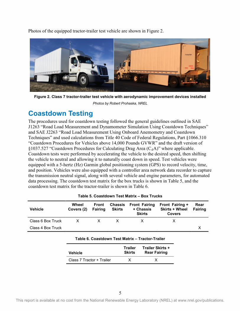
Photos of the equipped tractor-trailer test vehicle are shown in Figure 2.

Figure 2. Class 7 tractor-trailer test vehicle with aerodynamic improvement devices installed

Photos by Robert Prohaska, NREL

Coastdown Testing The procedures used for coastdown testing followed the general guidelines outlined in SAE J1263 “Road Load Measurement and Dynamometer Simulation Using Coastdown Techniques” and SAE J2263 “Road Load Measurement Using Onboard Anemometry and Coastdown Techniques” and used calculations from Title 40 Code of Federal Regulations, Part §1066.310 “Coastdown Procedures for Vehicles above 14,000 Pounds GVWR” and the draft version of §1037.527 “Coastdown Procedures for Calculating Drag Area (CdA)” where applicable. Coastdown tests were performed by accelerating the vehicle to the desired speed, then shifting the vehicle to neutral and allowing it to naturally coast down in speed. Test vehicles were equipped with a 5-hertz (Hz) Garmin global positioning system (GPS) to record velocity, time, and position. Vehicles were also equipped with a controller area network data recorder to capture the transmission neutral signal, along with several vehicle and engine parameters, for automated data processing. The coastdown test matrix for the box trucks is shown in Table 5, and the coastdown test matrix for the tractor-trailer is shown in Table 6.

Table 5. Coastdown Test Matrix – Box Trucks

Vehicle Wheel

Covers (2) Front

Fairing Chassis Skirts

Front Fairing + Chassis

Skirts

Front Fairing + Skirts + Wheel

Covers

Rear Fairing

Class 6 Box Truck X X X X X

Class 4 Box Truck X

Table 6. Coastdown Test Matrix – Tractor-Trailer

Vehicle Trailer Skirts

Trailer Skirts + Rear Fairing

Class 7 Tractor + Trailer X X


Testing was performed on a private stretch of road that runs parallel to the east runway at Front Range Airport, located east of Denver, Colorado. Figure 3 shows an aerial picture of the private road with the test section (approximately 1.2 miles long) highlighted in green, along with a picture from in the middle of the track looking north.

Figure 3. Coastdown test track

© Google Earth (left); photo by Adam Ragatz, NREL (right)

The track has a very slight grade (Figure 4), which is hard to perceive with the naked eye but has a clear effect on vehicle behavior, so the data needed to be corrected for grade during post processing. The processing code leverages either a manual land survey conducted by NREL staff or U.S. Geological Survey aerial light detection and ranging, known as LIDAR, elevation data for correction.

Figure 4. Coastdown track grade


A stationary roadside weather station, located just next to the coastdown test track, was used to collect 1-Hz wind speed, direction, temperature, pressure, and humidity data and was used to make corrections for weather conditions per the coastdown procedure (Figure 5). The Airmar 150WX weather station also has a built-in GPS and compass, which are used to report wind direction relative to magnetic and true north regardless of sensor orientation. GPS time is used to stitch vehicle telemetry and weather results together. The weather station is mounted directly on a tripod that was adjusted to approximately half the vehicle height. This roadside weather station was used for the box truck and “pup” trailer coastdown tests.

Figure 5. Stationary roadside weather station, Airmar 150WX

Photo by Adam Ragatz, NREL

In addition to the stationary roadside weather station, an on-board anemometer (YOUNG Model 81000 ultrasonic anemometer) was used to measure wind velocity as perceived by the moving vehicle during the tractor-trailer tests. The unit was mounted on the front of the trailer with the centerline approximately one meter above the top of the trailer, as shown in Figure 6. Additional measurements are shown in Appendix B.


Figure 6. On-board ultrasonic anemometer, YOUNG model 81000

Photos by Adam Ragatz, NREL

Coastdown tests were performed in both directions; due to the track’s slight grade, the northbound and southbound profiles differ. Figure 7 shows a sample of raw GPS data for 12 runs, six in each direction.

Figure 7. Raw GPS data from 12 coastdown runs (six in each direction)

North South


The following road load equation is used to describe the behavior of the vehicle:

𝐹𝐹 −𝑚𝑚𝑚𝑚 ∆ℎ∆𝑥𝑥

= 𝜇𝜇𝑚𝑚𝑚𝑚 + 12� 𝜌𝜌𝜌𝜌𝐶𝐶𝑑𝑑𝑉𝑉2 (1)

where F is the force due to road load, m is the vehicle mass, g is the gravitational constant, ∆ℎ∆𝑥𝑥

is the road grade, µ is the coefficient of rolling resistance, ρ is the density of air, A is the cross-sectional area, Cd is the drag coefficient, and V is the velocity.

At each time step interval, the total force on the vehicle can be calculated using Newton’s second law of motion where the external forces F on an object are equal to the mass m multiplied by the acceleration a of the object:

𝐹𝐹 = 𝑚𝑚𝑚𝑚 (2)

𝐹𝐹𝑖𝑖 = 𝑚𝑚𝑒𝑒𝑉𝑉𝑖𝑖−𝑉𝑉𝑖𝑖−1

∆𝑡𝑡 (3)

The effective mass (me) was calculated for the class 6 box truck and the tractor-trailer by adding 56.7 kilograms (kg) to the measured vehicle mass for each tire making road contact. For the class 4 box truck, the ratio of rotating mass to measured vehicle mass was kept the same as the class 6 box truck. After correcting for elevation change using the road grade survey, each interval point is plotted and a least-squares regression is used to determine the coefficients, as shown in Figure 8.

Figure 8. Example of road load force vs. vehicle speed and resulting fit curve


The least-squares regression follows the general form:

𝑓𝑓(𝑥𝑥) = 𝐶𝐶𝑥𝑥2 + 𝐵𝐵𝑥𝑥 + 𝜌𝜌 (4)

In the polynomial fit, the “B” term is fixed at zero and coefficients are assigned as follows:

𝜌𝜌 = 𝜇𝜇𝑚𝑚𝑚𝑚 (5)

𝐵𝐵 = 0 (6)

Switching nomenclature to match Title 40 Code of Federal Regulations §1066.310:

𝐶𝐶 = 𝐷𝐷 = 12� 𝜌𝜌𝜌𝜌𝐶𝐶𝑑𝑑 (7)

The “D” term can be corrected for standard conditions as follows:

𝐷𝐷𝑎𝑎𝑑𝑑𝑎𝑎 = 𝐷𝐷 𝑇𝑇293

98.21𝑃𝑃

(8)

On-Road Testing The procedure used for on-highway testing followed the general guidelines outlined in SAE J1526 “Joint TMC/SAE Fuel Consumption In-Service Test Procedure Type III.” On-road testing was conducted on a stretch of I-70 east of Denver, Colorado (Figure 9). The test and control vehicles entered the highway 30 – 60 seconds apart to experience the same traffic conditions, but not interfere with each other’s aerodynamics. Vehicles were accelerated until they reached the speed limit, at which point the cruise control was set and the fuel tank selector valves were switched from the main tanks to the test weigh tanks (Figure 10). Fuel consumption was accurately measured using a scale with 5-gram resolution, before and after each test run.


Figure 9. On-road test section © Google Maps

Figure 10. Secondary fuel weigh tank and scale



The SAE J1321 “Data Analysis – Fuel Economy Improvement Testing” utility was used to calculate the nominal fuel economy improvement and corresponding confidence interval from the raw fuel use data.

Results and Discussion Coastdown Testing – Box Trucks and Tractor-Trailer Coastdown road load force coefficients are shown in Table 7 and Table 8. Coefficient Am is a constant, independent of speed, and represents the rolling resistance component of road load force. Coefficient Dadj is the aerodynamic component of road load force, which depends on velocity squared. Dadj has been adjusted to standard temperature and pressure. These two coefficients can be used to solve for theoretical road load force at standard temperature and pressure and at any speed and are used to derive “Road Load @ XX mph (miles per hour)”. Finally, µ and CdA are derived by dividing out the other constants. Because the headwind / tailwind correction is derived from a stationary roadside weather station, the vehicle and weather station do not always experience the same conditions at the exact same time. Under steady weather conditions corrected results should provide a better estimate, but under changing conditions the wind correction has the potential to introduce additional error. For this reason results are presented both with and without wind correction for comparison. Table 7 uses ground speed as the velocity component, whereas Table 8 uses ground speed plus headwind or ground speed minus tailwind as the velocity component. Each colored grouping of tests was completed on the same day.

Table 7. Coastdown Results without Wind Correction

Error estimates shown are 95% confidence intervals.


Table 8. Coastdown Results with Wind Correction


Measured aerodynamic improvement for a specific device will depend on weather conditions. Some of these elements can be corrected for, as shown in Equation 8 and the headwind/tailwind aerodynamic velocity corrections in Table 8. However, other components such as crosswind and yaw angle are not accounted for in these corrections and may have a significant nonlinear effect that is difficult to correct for without additional data. For example, chassis skirts will demonstrate a higher advantage under high crosswind conditions. These advantages are real, but the test conditions need to be compared with average weather conditions where the device is intended to be deployed to understand how applicable the results will be. For this reason, average weather conditions, including wind vector components, for each test condition are shown in Table 9.

Table 9. Coastdown Average Weather Conditions


Using the data from the coefficients table, the observed percent change was determined by comparing the aerodynamic condition with the applicable baseline condition that day. Observed percent change for rolling resistance and aerodynamic coefficients, along with total road load, are shown with and without aerodynamic velocity wind correction in Table 10 and Table 11, respectively, and are displayed graphically in Figure 11 and Figure 12, respectively. A positive percent change and negative ΔCdA indicates an improvement, and therefore a reduction in drag. Similarly a negative percent change and positive ΔCdA represents an increase in drag. Changes in road load force should have an impact on vehicle fuel economy. The relative magnitude (i.e., percent change in fuel economy for a given percent change in road load force) is discussed further in the simulation section of this report. Estimated fuel economy improvement during transient conditions over standard drive cycles are also explored further in the Simulation Results section.

Table 10. Observed Change in CdA and Road Load without Wind Correction



Figure 11. Observed change in CdA and road load without wind correction.


Table 11. Observed Change in CdA and Road Load with Wind Correction



Figure 12. Observed change in CdA and road load with wind correction.


Both with and without wind correction, there was no statistically significant difference when adding the wheel covers for the box trucks. All other test scenarios showed a statistically significant change in total road load force in the 45–68 mph range. Both the front fairing and the chassis skirts show improvements on the order of 6% individually for total road load force. This was the highest of any individual component. When both devices are installed at the same time, the improvement increases to 8%–10%, greater than either individual component, but less than the sum of the two. The class 7 tractor-trailer demonstrated a roughly 2% improvement in road load force with trailer skirts only, and over 4% improvement with trailer skirts and a rear tail. The relationship between these results and modeled fuel economy improvement are explored in the Simulation section.

On-Road Testing – Box Trucks On-road testing was conducted for the box trucks to verify these theoretical fuel economy projections under real-world highway driving conditions. Table 12 shows results for individual testing days, all of which included a minimum of four test and four baseline runs. Combined, data such as “Chassis Skirts” is a combination of all test days (1–3). This is also shown graphically in Figure 13.


Table 12. On-Road Fuel Economy Test Results

Test Vehicle

Aerodynamic Device(s) Fuel Saveda

Fuel Economyb

Improvementc Avg

Temp Avg

Wind Speed

Nominal CId Nominal CId °F mph

Class 6 Box Truck Wheel Covers 0.30% 2.00% 0.30% 2.01% 66.6 7.7

Class 6 Box Truck Front Fairing 1 3.12% 3.16% 3.23% 3.26% 59.7 10.7

Class 6 Box Truck Front Fairing 2 4.19% 3.02% 4.37% 3.15% 53.7 6.6

Class 6 Box Truck Front Fairing 3.59% 1.79% 3.72% 1.86%

Class 6 Box Truck Chassis Skirts 1 8.34% 1.78% 9.09% 1.94% 60.5 21.9



Class 6 Box Truck Chassis Skirts 5.40% 1.64% 5.71% 1.73%

Class 6 Box Truck Wheel Covers + Front Fairing + Chassis Skirtse

3.23% 2.61% 3.34% 2.69% 50.9 8.6

Class 6 Box Truck Front Fairing + Chassis Skirts 7.66% 1.63% 8.30% 1.77% 63.1 6.6

Class 4 Box Truck Rear Fairing 3.31% 3.26% 3.43% 3.37% a “Fuel Saved” was calculated as ((baseline fuel used) – (test case fuel used)) / (baseline fuel used) b “Fuel Economy” was calculated as ((distance traveled) / (fuel used))

“Fuel Consumption” was calculated as ((fuel used) / (distance traveled)) c “Improvement” was calculated as ((test case) – (baseline)) / (baseline) d Error estimates shown are 95% confidence intervals. e “Wheel Covers + Front Fairing + Chassis Skirts” removed from graph due to changing weather conditions and

suspected erroneous data.


Figure 13. On-road fuel consumption test results

“Wheel Covers + Front Fairing + Chassis Skirts” not included due to changing weather conditions and suspected erroneous data.

Wheel covers again showed no statistically significant difference from the baseline for on-road testing as well. The measured fuel savings from the use of a front fairing, chassis skirts, a combination of both, and a rear fairing all fell in line with expectations from the theoretical road load predictions based on coastdown results. The “Wheel Covers + Front Fairing + Chassis Skirts” condition from Table 12 is suspected to be erroneous due to changing environmental conditions during testing. Because there was insufficient time to repeat this condition within our established testing window, it has been excluded from Figure 13. Chassis skirts had the most test repeats, capturing a broad range of wind conditions ranging from a slight breeze to strong and constant crosswinds. Figure 14 shows this range in fuel savings that can be realized under these different scenarios. Figure 15 shows California average wind conditions by month and hour of the day (top) and a combined histogram for wind speed year-round from 8 a.m. to 6 p.m. Wind data were supplied by the National Oceanic and Atmospheric Administration climate norms database and are an average of normal conditions at the Bakersfield, Los Angeles, San Diego, Sacramento, San Francisco, and Stockton airport weather stations. Looking at the California wind data alongside the chassis skirt wind dependence shows that fuel savings are going to vary throughout the day and seasonally.


Figure 14. On-road fuel savings from chassis skirts under various wind conditions

“Fuel Saved” was calculated as ((baseline fuel used) – (test case fuel used)) / (baseline fuel used). Error estimates shown are 95% confidence intervals.


Figure 15. California average wind speed


Simulation Results The following simulation examples are intended to explore the real-world fuel savings benefits that could be realized with aerodynamic improvement devices in various vocations, explore what vehicle characteristics, if any, correlated well with potential aerodynamic benefit, and reinforce how important duty cycle is on the final outcome. For a given vehicle, the simulated road load force is a function of both vehicle speed and mass. Equation 1, shown here again for reference, describes this behavior.

𝐹𝐹 −𝑚𝑚𝑚𝑚 ∆ℎ∆𝑥𝑥

= 𝜇𝜇𝑚𝑚𝑚𝑚 + 12� 𝜌𝜌𝜌𝜌𝐶𝐶𝑑𝑑𝑉𝑉2 (1)

To illustrate the dramatic effect weight can have on total road load force, a series of example coefficients have been selected. The following constants have been fixed: µ = 0.0062, g = 9.81 m/s2, ρ = 1.17 kg/m3, and Cd = 0.5. The road load components from three theoretical vehicles are shown in Figure 16. The cross-sectional area and empty/full weights selected for the class 4 and class 6 vehicles are identical to the test vehicles in this study. The cross-sectional area and empty/full weights for the class 8 vehicle were selected to match that of a typical on-road line-haul tractor-trailer.

Figure 16. Theoretical road load components. Aerodynamics are more important for lightly loaded

vehicles.


For a fully loaded class 8 tractor-trailer traveling at 60 mph, the rolling resistance and aerodynamic resistance are nearly equal. This means a modification to the aerodynamic drag coefficient of 1% would have an approximate 0.5% change to the total road load force since the components are equal and rolling resistance is unaffected. However, for a lightly loaded tractor-trailer, the aerodynamic component plays a greater role. For a class 6 box truck, the aerodynamics are very similar—it is the same width and only 8 inches shorter than the tractor-trailer (approximately 5% difference)—but the weight is substantially different: the class 6 box truck weighs approximately one-third of the weight of the tractor-trailer when both are full. Therefore, aerodynamics become even more important if those vehicles are expected to see a significant amount of highway operation. This is illustrated in Figure 17.

Figure 17. Percent change in fuel economy for a 1% change in Cd

“Fuel Economy” was calculated as ((distance traveled) / (fuel used)). “% Change” was calculated as ((test case) – (baseline)) / (baseline) x 100.

For a fully loaded class 8 tractor-trailer traveling at 60 mph, a 1% change in Cd is expected to result in an approximate 0.5% change in fuel economy. For a class 6 box truck traveling at 30 mph, a 1% change in Cd is expected to result in an approximate 0.25% change in fuel economy. However, if that same class 6 box truck is placed in a vocation where it averages 60 mph, this could result in an approximate 0.7% change in fuel economy. This emphasizes how important it is to pair these devices with a vehicle operating on an appropriate duty cycle to maximize fuel economy gains.

Using the coastdown results, theoretical fuel economy improvements can be predicted over steady-state conditions, and various transient drive cycles. The coastdown coefficients from Table 8 are used to populate a road load force curve. For a given drive cycle, assuming zero grade, the required force at each speed interval can be found using this curve. Some assumptions


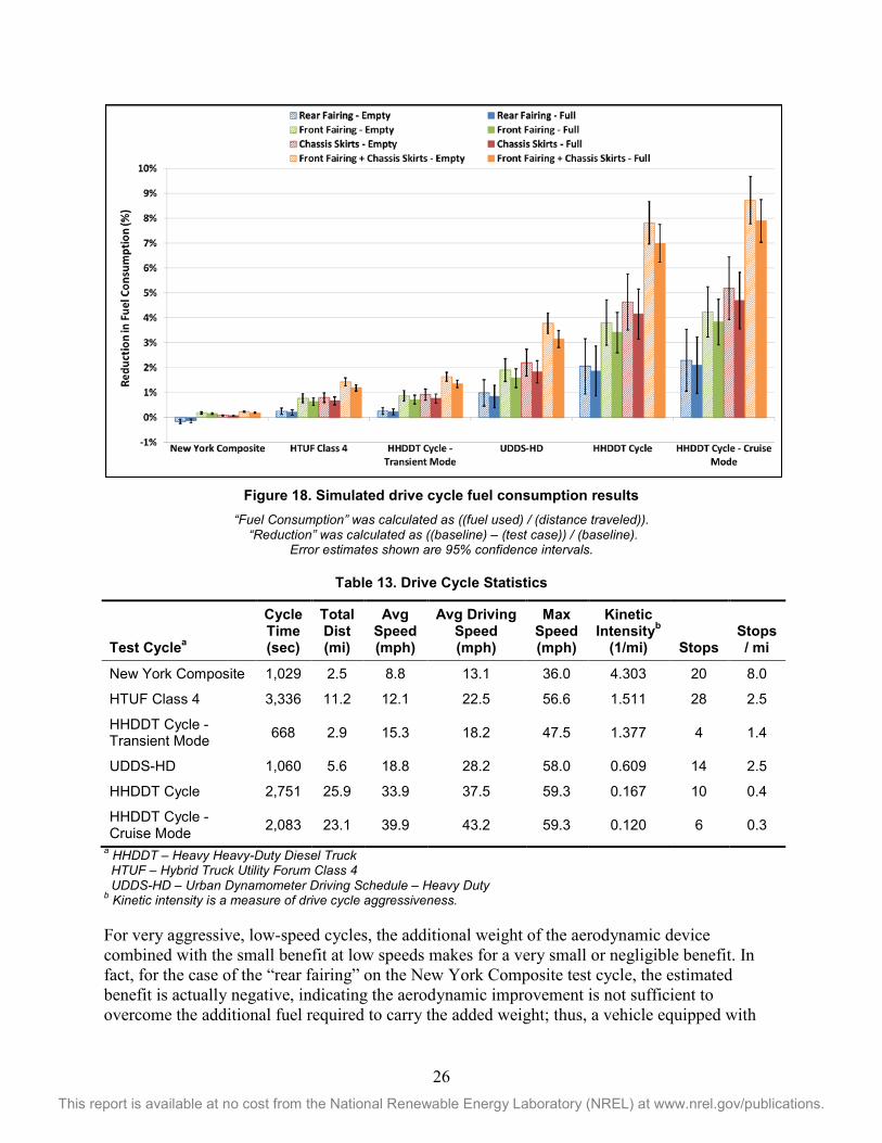
about driveline efficiency and an engine thermal efficiency curve can be used to derive instantaneous fueling requirements and eventually arrive at a full cycle fuel economy with the test device and for the baseline condition. Figure 18 shows four test scenarios, “rear fairing,” “front fairing,” “chassis skirts,” and “front fairing + chassis skirts,” respectively, at empty weight and maximum gross vehicle weight rating, along with a composite graphic for comparison across devices. The combination of front fairing and chassis skirts shows the greatest advantage across all cycles. The wheel covers are not shown since the results showed no statistically significant difference. Drive cycle statistics are shown in Table 13.




Figure 18. Simulated drive cycle fuel consumption results

“Fuel Consumption” was calculated as ((fuel used) / (distance traveled)). “Reduction” was calculated as ((baseline) – (test case)) / (baseline).


Table 13. Drive Cycle Statistics

Test Cyclea

Cycle Time (sec)

Total Dist (mi)

Avg Speed (mph)

Avg Driving Speed (mph)

Max Speed (mph)

Kinetic Intensityb

(1/mi) Stops Stops/ mi

New York Composite 1,029 2.5 8.8 13.1 36.0 4.303 20 8.0

HTUF Class 4 3,336 11.2 12.1 22.5 56.6 1.511 28 2.5

HHDDT Cycle - Transient Mode 668 2.9 15.3 18.2 47.5 1.377 4 1.4

UDDS-HD 1,060 5.6 18.8 28.2 58.0 0.609 14 2.5

HHDDT Cycle 2,751 25.9 33.9 37.5 59.3 0.167 10 0.4

HHDDT Cycle - Cruise Mode 2,083 23.1 39.9 43.2 59.3 0.120 6 0.3

a HHDDT – Heavy Heavy-Duty Diesel Truck HTUF – Hybrid Truck Utility Forum Class 4 UDDS-HD – Urban Dynamometer Driving Schedule – Heavy Duty b Kinetic intensity is a measure of drive cycle aggressiveness.

For very aggressive, low-speed cycles, the additional weight of the aerodynamic device combined with the small benefit at low speeds makes for a very small or negligible benefit. In fact, for the case of the “rear fairing” on the New York Composite test cycle, the estimated benefit is actually negative, indicating the aerodynamic improvement is not sufficient to overcome the additional fuel required to carry the added weight; thus, a vehicle equipped with


this device on this cycle would actually consume more fuel. However, for cycles with significant highway contributions, the benefits can be much more substantial. It is important when considering aerodynamic improvement devices for vocational vehicles, that they are paired with an appropriate drive cycle to realize the maximum benefit.

To better understand how devices like these could perform under real-world driving conditions and to determine which vehicle characteristics were most correlated with high potential aerodynamic benefits, a similar simulation approach was used, but rather than using standard drive cycles the results were simulated over real-world driving days. This analysis leveraged real-world vocational vehicle activity data already collected under NREL’s Fleet DNA commercial vehicle database.3 This online tool provides data summaries and visualizations for medium- and heavy-duty commercial fleet vehicles operating in a variety of vocations. CARB was also interested in whether these results could leverage recent work NREL conducted in collaboration with the U.S. EPA under Interagency Agreement IAG-14-1954 covering “The Development of Vocational Vehicle Drive Cycles and Segmentation.”4 This analysis was used to help guide the U.S. EPA’s methodology and approach for the proposed Phase 2 Greenhouse Gas Emissions Standards.5 The simulation tool used for the following analysis was NREL’s Future Automotive Systems Technology Simulator (FASTSim).6 FASTSim is a power-based rapid screening tool used to evaluate the impact of technology improvements on efficiency, performance, and cost in conventional and hybrid vehicles. This approach involved selecting a subset of the Fleet DNA data used for the U.S. EPA analysis that would have similar vehicle characteristics to the types of vocational vehicles tested during this aerodynamic drag reduction study. Four FASTSim vehicle models were developed and tuned to real-world data: large box truck (class 6–7), small box truck (class 3–5), step van (class 4–5), and a vocational tractor-trailer (class 7–8). The most relevant vehicle data for each subgroup were lumped together to form a FASTSim model for each group. Each model was tuned by feeding a 1-Hz speed trace through the simulation along with the vehicle model to obtain a theoretical 1-Hz fueling trace. The theoretic fuel trace from the model was compared with the actual 1-Hz J1939 fuel data collected in the field. Then, using a least squares approach, parameters of the model were iterated on to reduce the error between the theoretical and real-world data. This was done for various vehicles over many days of operation to arrive at a model that most closely represented an average vehicle in each group. An example of this parameter sweeping exercise is shown in Figure 19 for one case, the step van.

3 Fleet DNA: Commercial Fleet Vehicle Operating Data, http://www.nrel.gov/transportation/fleettest_fleet_dna.html 4 Vocational Vehicle Drive Cycle Data: Draft Report produced by the National Renewable Energy Laboratory entitled The Development of Vocational Vehicle Drive Cycles and Segmentation, https://www.regulations.gov/#!documentDetail;D=EPA-HQ-OAR-2014-0827-1621 5 Greenhouse Gas Emissions Standards and Fuel Efficiency Standards for Medium- and Heavy-Duty Engines and Vehicles (Phase 2), https://www.regulations.gov/#!docketDetail;D=EPA-HQ-OAR-2014-0827 6 Future Automotive Systems Technology Simulator, http://www.nrel.gov/transportation/fastsim.html

http://www.nrel.gov/transportation/fleettest_fleet_dna.html

https://www.regulations.gov/%23!documentDetail;D=EPA-HQ-OAR-2014-0827-1621

https://www.regulations.gov/%23!docketDetail;D=EPA-HQ-OAR-2014-0827

http://www.nrel.gov/transportation/fastsim.html


Figure 19. Model tuning – step van

The error in this case is the total sum of 1-Hz differences squared over all vehicle days. However, a more tangible way of looking at this would be to rerun the tuned model over all driving days and compare the theoretical total daily fuel use with what was reported by J1939 during field data collection. This is done in Figure 20 for the step van results with a coefficient of determination equal to 0.9377 representing the goodness of fit for this model to all 60 real-world vehicles with 1,096 combined days of operation. The coefficients of determination for the vocational tractor and large box truck models were 0.9219 and 0.9297 respectively. Due to a lack of sufficient real-world small box truck activity data, the small box truck model was constructed using the tuned large box truck model with CdA and mass scaled by the same ratio as the test vehicles for this study. Therefore, the underlying real-world tuning data for both box truck models is the same.

Table 14 shows the final tuned CdA and vehicle mass for each model along with the total number of vehicles and combined driving days used for tuning.

Figure 20. Theoretical vs. J1939 daily fuel for step vans

Min Error


Table 14. Tuned Model Results

Model Parameters Tuning Data

Vehicle Model CdA (m2) Mass (lbs.) Vehicles Days

Vocational Tractor 7.1 26,400 7 101

Large Box Truck 5.4 21,120 23 393

Small Box Truck 4.8 10,890 23 393

Step Van 3.6 11,528 60 1,096

These models were then used to explore theoretical fuel saving resulting from a change in CdA. The two hypothetical scenarios chosen were a 5% and 10% reduction in CdA. For scenarios showing a payback period, it was assumed the 5% improvement would cost $1,000 and a 10% improvement would cost $2,500. This was roughly in agreement with the price vs. improvement observed in this study, but a much more rigorous analysis would need to be conducted to estimate real-world return on investment, including installation and maintenance costs, as well as mass market pricing for these devices since some were adapted from line-haul applications. Also, the real-world drive cycles used for simulation were not intended to be representative of the entire California vocational market, but rather a sampling of examples which could be used to guide future analysis. Current U.S. Energy Information Administration projections estimate diesel fuel will average $3.17 a gallon in the year 2020 and current California on-road diesel prices average just over 14% higher than the rest of the nation.7 Therefore, an assumed constant price of $3.63 per gallon was used as a California 2020 projection when converting between gallons displaced and dollars saved.

Each vehicle model was operated over the corresponding days of vehicle operation used for tuning to establish the baseline conditions. Then the CdA value was reduced to 95% and finally 90% of the original value for the two test cases. Figure 21 shows both a probability and cumulative gamma fit to the large box truck results for these two scenarios. The area shaded in green indicates the percentage of vehicles which could be expected to see a payback period of 4 years or less (for example, 10.3% of large box trucks would have fuel savings enough for a 5% CdA improvement to give a payback period of 4 years or less). Since the 10% CdA reduction device costs more than twice as much, a smaller percentage of vehicles are able to achieve payback during the prescribed period, but on average they will displace more fuel. Note that vehicles to the left of the payback line, making up the majority, do see some benefit, but it is not substantial enough to achieve a 4-year payback.

7 Short-Term Energy Outlook, https://www.eia.gov/forecasts/steo/report/prices.cfm

https://www.eia.gov/forecasts/steo/report/prices.cfm


Figure 21. Large box truck simulation results. Probability distribution (left) and cumulative

distribution (right)

Displacing fuel burned by the engine not only saves money in fuel cost, but also has a direct impact on the amount of carbon dioxide released at the tailpipe. An assumed value of 10.18 kg carbon dioxide per gallon of diesel fuel was used to convert displaced gallons into greenhouse gas impacts.8 Simulation results for a 5% and 10% aerodynamic improvement are shown in Figure 22 for the large box truck model.

Figure 22. Large box truck simulation results – cumulative distribution of potential greenhouse

gas savings

Table 15 presents the payback in years for 5% and 10% improvements in CdA for several types of vehicles. Figure 23 shows the simulated annual fuel saving distributions for all models over the corresponding real-world drive cycles, for both a 5% and 10% aerodynamic improvement. The tables at the top of the figure show the estimated percentage of vehicles in each category that would be expected to achieve a payback within the specified number of years. It is important to 8 Greenhouse Gas Emissions from a Typical Passenger Vehicle, https://www3.epa.gov/otaq/climate/documents/420f14040a.pdf

https://www3.epa.gov/otaq/climate/documents/420f14040a.pdf


note that the payback analysis only includes an estimated cost for the device(s), and does not include installation, periodic maintenance, or replacement due to accidental damage throughout its life. This analysis is also specific to the data available through NREL’s Fleet DNA and is not necessarily representative of the entire California vocational vehicle market. To fully understand the real-world payback period a more rigorous analysis would have to be conducted.

Table 15. Device Payback Period

5% CdA Improvement ($1,000) 10% CdA Improvement ($2,500)

Payback (years) 2 4 8 2 4 8

Large Box Truck 0.7% 10.3% 37.2% 0.2% 5.1% 26.1%

Small Box Truck 0.4% 7.9% 33.2% 0.1% 3.6% 22.2%

Step Van 0.0% 0.4% 9.7% 0.0% 0.1% 4.3%

Tractor 13.2% 37.8% 63.1% 7.4% 28.2% 54.5%

Figure 23. Simulation results – all models, 5% CdA improvement (left), 10% CdA improvement

(right), probability distributions (top), cumulative distributions (bottom)

Next we explored the relationship between fuel saved on a percentage basis and total gallons displaced. For a fixed percentage improvement, vehicles that naturally consume more fuel will


see a greater total absolute number of gallons displaced. However, even for a large percentage improvement, vehicles that do not travel a significant distance each day or are only operated periodically will not displace a large number of total gallons. For this reason, fuel savings on a percentage basis and absolute number of gallons displaced are related, but not by a one-to-one relationship. Figure 24 shows simulation results both ways, color coded by model, with fit curves for a 5% CdA improvement. Each data point represents one real-world vehicle day of operation. Note that on average the heavier vocational tractor-trailer results are shifted to the right, indicating more total gallons displaced for a given percentage; the lighter small box truck is shifted to the left, indicating less total gallons displaced for a given percentage, as expected.

Figure 24. Daily fuel saved – gallons vs. percentage for a 5% CdA improvement

Figure 25 shows these results as cumulative gamma fit distributions both ways. Again, the heavier vocational tractor-trailer model shows the greatest benefit on a total-gallon basis (left) and has a significant ~50% of vehicles that would achieve a 5-year payback. The lighter small box truck demonstrates a significant percentage improvement (right) because aerodynamics makes up a more significant portion of its fuel use and thus a fixed improvement to CdA has a more substantial impact on a percentage basis. The bins indicated on the percentage improvement plot (right) were provided by CARB as initial groupings of interest. The intervals are defined in Table 16.

Table 16. Percentage Improvement Bins

Bin % Fuel Saving

I [0%, 1%)

II [1%, 2.5%)

III [2.5%, 5%]


Figure 25. Simulation result for a 5% CdA improvement, cumulative distributions – total gallons

(left), percent savings (right)

To implement any type of program that would utilize aerodynamic improvement devices on vocational vehicles, it is important to understand which vehicles and drive cycles would realize the greatest benefit to maximize cost effectiveness. Figure 26 shows drive cycle aggressiveness (kinetic intensity) vs. average speed for each day of real-world driving. Simulated results indicating bin III (2.5% – 5% fuel savings) shown above, are highlighted in yellow.

Figure 26. Kinetic intensity vs. average speed

Kinetic intensity appears to play a strong role in predicting significant savings and average speed also plays a role but with considerably more spread. This is highlighted in Figure 27 where the same results are plotted against fuel savings with fit curves. Average speed demonstrates a trend,


but not near as strong as kinetic intensity. Engine speed in top gear at 65 mph was one of the primary metrics used to predict vehicle cluster for the U.S. EPA clustering analysis, but proves to be a rather poor indicator of aerodynamic improvement benefit.

Figure 27. Simulation drive cycle trends – fuel savings vs. average speed, kinetic intensity, and

engine speed at 65 mph


The three mode clusters used for the U.S. EPA analysis are shown in the upper left of Figure 28. The low-speed, highly aggressive cluster 1 is shown in green; the high-speed, steady cluster 3 is shown in purple. Cluster 2 falls in between; for more explanation of the clusters, please refer to the draft report.9 The black data points indicate the vehicle days used for this simulation analysis. The vehicle days highlighted in red indicate the largest fuel savers on a “total gallons” basis, and the points highlighted in yellow indicate the vehicle days that saw the greatest fuel savings benefit on a percentage basis. In general, the vehicle days observing the largest benefits are shifted to the right, towards the high-speed cluster, which would be expected, but a considerable amount of spread indicates cluster alone may not be enough information to predict fuel savings from the addition of an aerodynamic improvement device.

Figure 28. U.S. EPA cluster analysis, Cluster 1: low-speed, aggressive (green); Cluster 2: mid-

speed (orange); Cluster 3: high-speed steady (purple); driving days used for this reports analysis (black); biggest fuel savers on a “total gallon” basis (red); biggest fuel savers on a percentage

basis (yellow)

9 Vocational Vehicle Drive Cycle Data: Draft Report produced by the National Renewable Energy Laboratory entitled The Development of Vocational Vehicle Drive Cycles and Segmentation, https://www.regulations.gov/document?D=NHTSA-2014-0132-0187

https://www.regulations.gov/document?D=NHTSA-2014-0132-0187


Vehicle days were then subdivided by vocation. Figure 29 shows the range in kinetic intensity and average speed observed by each vocation and the corresponding clusters it spans. Two notes appearing on both sets of charts highlight points of interest. First, how the same vehicle (class 4–5 step van) can have significantly different drive cycle statistics and cluster location just based on the vocation in which it is deployed, e.g., parcel vs. linen delivery. Second, both warehouse and beverage delivery vocations demonstrated a relatively broad range in activity for the number of days considered, spanning all three clusters. This indicates those vocations could have a broad range in fuel savings from aerodynamic improvement; however, caution should be taken to focus on vehicles that would see the greatest benefit to maximize effectiveness.


Figure 29. Vehicle activity and cluster by vocational grouping, all vehicle days considered (black),

member of the specified vocation (yellow)


Conclusion Testing results have indicated adding an aerodynamic improvement device or combination of devices to certain types of vocational vehicles can result in a measurable fuel economy improvement. However, the precise benefit realized under real-world driving conditions is strongly dependent on the vehicle drive cycle. Because vocational vehicles are used in such a wide array of applications, vehicle build specifications alone may not be sufficient to predict aerodynamic benefit. However, certain drive cycle characteristics such as kinetic intensity have demonstrated a very strong prediction capability. Therefore, before moving forward with the implementation of aerodynamic improvement technologies on any set of vocational vehicles, it is important to understand the target vocation and duty cycle as they significantly impact the potential benefits of the technology and the associated payback period. The vehicles examined in this study—class 7 and 8 beverage delivery tractors along with step vans deployed on routes with significant high speed and low kinetic intensity operation—saw the greatest benefit. While parcel delivery step vans and box trucks deployed on low speed, highly aggressive routes saw the worst performance benefit from reducing aerodynamic drag.

Note on additional testing: In addition to the aerodynamic drag reduction testing and analysis presented in this report, a series of tests examining the relationship between J1667 snap acceleration exhaust opacity and engine Federal Test Procedure PM levels for a partially failed diesel particulate filter was conducted under the same contract. Those results are summarized in Appendix C.


Appendix A – Additional Truck Dimensions Class 6 Box Truck





Class 4 Box Truck





Appendix B – Additional Tractor-Trailer Dimensions


Image by Southwest Research Institute


Appendix C – Heavy-Duty On-Road Vehicle Opacity and Engine Repair Durability In addition to the aerodynamic work presented above, under the same contract, NREL performed a series of tests exploring the relationship between snap acceleration smoke opacity and gravimetric particulate matter (PM) collected during the engine Federal Test Procedure (FTP). The tests were performed downstream of a partially failed diesel particulate filter (DPF) and repeated with varying degrees of failure. DPFs, which are now standard on all new heavy-duty diesel engines produced and certified starting in 2007, exhibit filtration efficiencies greater than 90%.10 However, the smoke opacity limit has not been revised since the widespread adoption of these filters. The goal of this work was to establish an empirical relationship between snap acceleration smoke opacity and gravimetric PM over the certification cycle for two engines at the NREL Renewable Fuels and Lubricants (ReFUEL) laboratory, a 2012 Cummins ISL and a 2008 MaxxForce 10. In addition to this comparison, a number of other real-time particle instruments were included for evaluation.

Background The CARB, under the Heavy-Duty Vehicle Inspection Program and Periodic Smoke Inspection Program, conducts routine checks of in-service vehicles for compliance. These checks are typically carried out at a weigh station or state border crossing. The smoke test procedure used is the SAE J1667 “Snap Acceleration Smoke Test Procedure for Heavy-Duty Powered Vehicles.”11 This procedure begins with one enforcement officer explaining the procedure to the vehicle driver while the other officer(s) prepare the equipment. When everyone is ready, the opacity meter is zeroed, then placed in the exhaust stream at the end of the tailpipe. The officer gives the command, and the driver snaps the accelerator pedal all the way to the floor and holds for approximate 4 seconds. The opacity meter records the peak opacity measurement per the filtering procedure outlined in J1667. This process is then repeated for a total of three practice snaps and three test snaps. The raw opacity measurements are corrected for ambient temperature, humidity, and barometric pressure. The average of the corrected values must fall below the applicable standard or the vehicle fails. The long-standing peak opacity limits for heavy-duty vehicles with engine model year 1990 and older has been 55% and 40% for 1991 and newer. It is anticipated that failure of the current gravimetric PM limit over the FTP certification cycle will occur far below these values for a modern DPF-equipped HD engine.

Instrumentation A full list of SAE J1667-approved smoke opacity meters is available from CARB’s website: http://www.arb.ca.gov/enf/hdvip/smokemtr.htm. For this report, the manufacturers’ names have been removed, and the test meters will be referred to as units A, B, C, and D. Units A, B, and D are certified meters listed on the website above. Unit C was a prototype supplied by the manufacturer. Unit D was an inline meter and was used during all engine FTP tests.

10 Diesel Particulate Filters, https://www.dieselnet.com/tech/dpf.php 11 Snap-Acceleration Smoke Test Procedure for Heavy-Duty Diesel Powered Vehicles, http://www.arb.ca.gov/enf/hdvip/saej1667.pdf

http://www.arb.ca.gov/enf/hdvip/smokemtr.htm

https://www.dieselnet.com/tech/dpf.php

http://www.arb.ca.gov/enf/hdvip/saej1667.pdf


In addition to opacity measurements, the snap acceleration tests included total solid particle number measurements from diesel-powered vehicles using a TSI nano particle emissions tester (NPET) model 3795. This is a portable unit intended to be used as a field regulatory inspection and maintenance instrument.12 Engine FTP tests included polytetrafluoroethylene membrane gravimetric PM filters sampled from a constant volume sampler (CVS) tunnel with the filter face temperature maintained at approximate 50°C. The gravimetric filters were used as the standard since this is the process used for certification. However, filters only provide one data point per test, so additional real-time instruments were included for time series comparison with the inline opacity meter and to each other. The AVL 483 micro soot sensor (MSS) is a photoacoustic soot measurement sensitive to black carbon and is equipped with its own diluter. Other benchtop instruments were positioned downstream of a Dekati fine particle sampler, which is a commercial partial flow dilution system for fine particle measurements. Instruments positioned after the Dekati fine particle sampler included a TSI 3776 condensation particle counter (CPC), TSI 3090 engine exhaust particle sizer (EEPS), TSI 8533 DustTrak DRX, and finally the NPET. Figure 30 shows a schematic of the instrumentation test setup.

Figure 30. Instrumentation test setup

Test Plan The series of tests that were carried out were designed to simulate a minor DPF failure up through gross failure and even complete removal. The two main test platforms were the NREL ReFUEL laboratory’s heavy-duty engine dynamometer and a transit bus with the same engine and emissions family. Testing began with a 2013 transit bus, which was later replaced by a 2011 transit bus for the official tests. Figure 31 outlines the various testing platforms with the bulk of the testing being carried out on the middle two (highlighted in orange). The procedure included

12 TSI Precision Measurement Instruments, http://www.tsi.com/

http://www.tsi.com/


running three engine FTP tests on the engine dynamometer and then swapping the test filter into the transit bus and conducting the J1667 snap acceleration test in the field following the same procedure as a real-world test. The filter was then progressively failed by milling off channel end caps and the process was repeated until an acceptable level of failure was reached. Finally, a series of FTP and snap acceleration tests were conducted on an engine test cell platform only to demonstrate the potential difference between a DPF + selective catalyst reduction strategy vs. a DPF only strategy. This is outlined graphically below.

Figure 31. Testing platforms

Photos/images by Adam Ragatz, NREL

Ceramic wall-flow filters work by allowing engine exhaust gas to pass through an open channel with alternating and opposite channels plugged on the other side. This forces the gas flow to pass through the porous wall so it can exit out an adjacent channel. This is depicted graphically in the upper-right corner of Figure 32. By milling off channel end caps gas is allowed to freely flow down that channel without passing through the ceramic wall. Plugs were removed using an end mill. This process, along with a number of examples of failure levels for the Cummins DPF, is shown in Figure 32.


Figure 32. DPF progressive failure

Photos by Adam Ragatz, NREL and Corning Inc. (Upper-Right)

Results Results of the Cummins ISL tests are shown in Figure 33. The raw peak opacity and atmospheric condition corrected measurements for each level of failure are shown on the left. Each bar represents the average of all measurements made at each level and the error bars are the standard deviation of those measurements. Shown on the right are the analogous engine test cell measurements over the FTP for the gravimetric filters and integrated AVL MSS.

Figure 33. Cummins ISL results. Snap opacity (left) and engine FTP (right)


Notice that the repeatability on the engine FTP tests is much tighter than the opacity measurements, and the gravimetric filters and integrated AVL MSS exhibit excellent agreement over the full range of measurements. Figure 34 shows this agreement along with a fit curve. Error bars are shown as the standard deviation of these measurements over three FTP hot-start tests. As indicated earlier, the gravimetric filter samples and integrated AVL MSS are in excellent agreement and can be used interchangeably for this analysis.

Figure 34. Gravimetric filter vs. integrated AVL MSS

In Figure 33, the bar labeled “Upstream” measured the engine-out level by moving the MSS upstream while leaving the DPF in place so as to not trigger any engine faults. The upstream measurement can be used to project the expected opacity reading by completely removing the DPF without actually performing this test. This was done as a projection because it was anticipated that complete removal may trigger an engine fault and change the operating mode of the engine. Figure 35 shows this relationship between the AVL MSS and J1667 snap opacity, where each data point is an actual measurement with the exception of the dot highlighted in yellow which is an extrapolation for the upstream measurement. The confidence region highlighted in blue represents a second-order fit to the upper and lower confidence bounds. The graph on the left shows the average uncorrected raw opacity measurements at each failure condition while the graph on the right includes opacity correction for ambient conditions.


Figure 35. FTP vs. opacity fit curves

The red line denotes the current heavy-duty certification limit of 0.01 grams per brake horsepower-hour (g/bhp-hr), and the fit curve intersects the red line at around 2.8% opacity (corrected). It is important to note that this is only applicable for this engine and margins of error for engine-to-engine variability and instrument-to-instrument variability would have to be built into a revision of the standard. Therefore, for the next series of tests the heavy-duty engine was switched to a 2008 MaxxForce 10, which adheres to the same PM standard but uses a different NOx reduction strategy resulting in significantly different engine-out PM levels. The 2008 MaxxForce 10 engine uses a DPF only in conjunction with exhaust gas recirculation for reducing NOx emissions. Results for the MaxxForce engine are shown with the Cummins ISL results in Figure 36. Highlighted in yellow is the engine out PM level projections for both engines. The DPF-only technology is about twice as high due to NOx-PM tradeoffs as expected.

Figure 36. Results – MaxxForce 10 (blue), Cummins ISL (red)

An instrumentation comparison was conducted between the various instruments used during engine dynamometer FTP testing to examine the correlations between different time-series


measurement technologies. Figure 37 shows that in general the particle number instrumentation was in good agreement and the particle mass/volume instrumentation was in good agreement, but the relationship between the two was weaker. The inline opacity meter had a relatively good correlation with the AVL MSS, but not near as strong as the TSI DustTrak and engine exhaust particle sizer (EEPS) total volume. The DustTrak especially is of particular interest because it is a lower cost technology that has already been proven to be rugged in the field.

Figure 37. FTP instrumentation correlogram

An instrumentation comparison was conducted among four different opacity meters and the AVL MSS during snap acceleration testing to show the agreement between units. Figure 38 shows that all units exhibit a similar trend with unit B reading slightly higher and unit C reading slightly lower at the higher concentrations, on average. Error bars indicate the standard deviation between measurements at each level of failure. The spread is similar across units, with unit D demonstrating the best repeatability. It should be noted that units A, B, and D were all certified meters, but unit C was a prototype.

Figure 38. Instrumentation comparison


Using the trend lines from the results presented here, projections of the level at various degrees of failure relative to the FTP PM emission standard could be made and are presented in Figure 39.

Figure 39. Failure level projections

Conclusion A series of tests exploring the relationship between J1667 snap opacity and engine dyno FTP levels were explored on two different engines at NREL’s ReFUEL laboratory. Both engines reached two times the FTP standard below 5% opacity (corrected) and had engine-out levels well below the current 40% limit. This is a strong indication that there may be room to tighten this standard for modern DPF-equipped engines. However, only two engines were tested, and they are not necessarily representative of the entire California fleet. Further work could be done to better understand the true variability from on-road vehicles in the state of California in support of this effort.

Documents

Aerodynamic Drag Reduction Technologies Testing of … · aerodynamic devices on select vocational vehicles and trailers, as accurately as possible given limited test time and budget