Embed Size (px)
Citation preview

AEA 303 AGRICULTURAL PRODUCTION ECONOMICS
114
AEA 303
;;;;;;;;;;;;;;;;;;;;;;;;;;;;;;;;;;;;;;;;;;;;;;;;;;;;;;;;;;;;;;;;;;
AEA 303: AGRICULTURAL PRODUCTION ECONOMICS
Course Team Dr. S.J. Ibitoye (Assoc. Professor) (Course
Writer/Course Developer)-Department of
Agricultural Economics and Extension, Kogi State
University Anyigba, Nigeria.
Professor N.E. Mundi (Course Editor/Programme
Leader) NOUN
Dr Kaine Anthony (Course Coordinator) NOUN
NATIONAL OPEN UNIVERSITY OF NIGERIA
National Open University of Nigeria
Headquarters
14/16 Ahmadu Bello Way
Victoria Island, Lagos
Abuja Office
5 Dar es Salaam Street
Off Aminu Kano Crescent
Wuse II, Abuja
e-mail: [email protected]
URL: www.nou.edu.ng
Published by
National Open University of Nigeria
Printed 2016
ISBN: 978-058-001-X
All Rights Reserved
Printed by
COURSE
GUIDE

AEA 303 MODULE 5
115
CONTENTS PAGE
Introduction ………………………………………………… iv
What You Will Learn in This Course ………………………. v
Course Aims …………………………………………………. vi
Course Objectives …………………………………………… vi
Course Requirements ……………………………………….. vii
Course Materials ……………………………………………... vii
Study Units ………………………………………………….. viii
Textbooks and References ………………………………….. ix
Assessment ………………………………………………….. x
Tutor-Marked Assignment …………………………………. x
Final Examination and Grading ……………………………. x
Summary ……………………………………………………. x
AEA 303 AGRICULTURAL PRODUCTION ECONOMICS
116
INTRODUCTION
AEA 303: Agricultural Production Economics is a one semester two (2)
credit units course designed for 300 level students. The course is
designed for the undergraduate students in the school of Agricultural
Sciences. The course will expose you to an understanding of many
concepts in Agricultural Production Economics. The knowledge gained
in this course will assist you to advise farmers and policy makers on the
most profitable level of farm production.
The course consists of two major parts, i.e. The Course Guide and The
Study Guide. The Study Guide consists of five modules and eighteen
units. The modules and the units under them are listed below:
Module 1 Nature of Agricultural Production Economics
Unit 1 Meaning and Scope of Agricultural Economics
Unit 2 Meaning and Scope of Agricultural Production Economics
Unit 3 Concepts in Agricultural Production Economics
Unit 4 Characteristics Features of Agricultural Production
Module 2 Theory of Production Economics
Unit 1 Meaning and Uses of Production Economics
Unit 2 Expression of Production Function
Unit 3 Functional Forms of Production Function
Unit 4 Time Periods in the Production Process
Module 3 Factor-Product Relationship
Unit 1 Laws of Returns
Unit 2 Classical Production Function
Unit 3 Output and Profit Maximization under One Variable Input
Unit 4 Resource Allocation Involving More Than One Variable
Input
Module 4 Factor-Factor and Product-Product Relationships
Unit 1 Profit Maximization in Factor-Factor Relationship
Unit 2 Important Concepts in Factor-Factor Relationship
Unit 3 Product-Product Relationship
Module 5 Production Costs
Unit 1 Meaning and Types of Cost

AEA 303 MODULE 5
117
Unit 2 Farm Cost Functions
Unit 3 Cost Functions and Production Function
This course guide tells you briefly on what the course is all about, what
course materials you will be using and how you can work your way
through these materials with minimum assistance. It suggests some
general guidelines for the amount of time you might spend in order to
successfully complete each unit of the course. It also gives you some
guidance on your Tutor Marked Assignment (TMA). Details of this
TMA will be made available in the assignment file. There are regular
tutorial classes that linked to the course. You are therefore advised to
attend to this session regularly.
WHAT YOU WILL LEARN IN THIS COURSE
AEA 303: Agricultural Production Economics consist of five major
components arranged in modules:
Nature of Agricultural Production Economics
Theory of Production Economics
Factor-Product Relationship
Factor-Factor and Product-Product Relationship
Production Costs
The first part which is on the nature of agricultural production
economics will introduce you into some concepts and background of
agricultural production economics. Issues discussed in unit one includes:
meaning and scope of agricultural economics and uses of economics in
agriculture. In unit two, you will look at the meaning and scope of
agricultural production economics. Unit three of the first part of the
study guide discussed some important concepts vital to the
understanding of this course. Some of the concepts include: production,
efficiency, variables, slope, coefficients, e.t.c. The last unit of the first
part focused attention on the characteristic features of agricultural
production.
Theory of production economics forms the major part of our discussion
in the second module. Unit 1 of that part will be devoted to the meaning
and uses of production economics. The second unit will cover the
expression of production function. Functional forms of production
function will occupy unit three of this module and the fourth unit will
discuss the time periods in the production process.
The third part of this course, which is on factor-factor relationship, is
divided into four units. Unit 1 will look at the laws of returns while unit
two will focus on the classical production function. Unit three of this
third part of the course will explain step by step how to calculate output

AEA 303 AGRICULTURAL PRODUCTION ECONOMICS
118
and profit maximization under one variable input. The last unit of this
part (unit 4) will explain resource allocation involving more than one
variable input.
The fourth part of the course will focus on factor-factor and product-
product relationships. This part will be discussed under three units. Unit
one will focus on profit maximization under factor-factor relationship.
The second unit of the module will explain some important concepts in
factor-factor relationship. Unit three of this part will discuss all the
various aspects of product-product relationship.
The last part of the course will focus on the production cost. This part
will be in three units. Unit one will look at the meaning and types of
costs. Unit two will look at the various aspects of farm cost functions.
Such aspects will include: total cost, fixed cost, variable cost and
marginal cost. Unit three which rounded up the course will look at the
relationship between cost functions and production functions.
COURSE AIMS
The aim of this course is to give understanding of the meaning of
various concepts of agricultural production economics. This aim will be
achieved by trying to:
explain the nature of agricultural production economics
describe the theory of production economics
outline the relationships between factor and product
explain the relationships between two factors in production
process
explain the relationships between two products in production
process
describe the concept of production cost
OBJECTIVES
In order to achieve the aims of this course, there are sets of overall
objectives. Each unit also has specific objectives. The unit objectives are
always included in the beginning of the unit. You need to read them
before you start working through the unit. You may also need to refer to
them during your study of the unit to check your progress. You should
always look at the unit objectives after completing a unit. In doing so,
you will be sure that you have followed the instruction in the unit.
Below are the wider objectives of the course as a whole. By meeting
these objectives you should have achieve the aims of the course as a
whole. On successful completion of the course, you should be able to:

AEA 303 MODULE 5
119
define agricultural economics and agricultural production
economics
give the various types of production function
identify time periods in production process
calculate the output and profit maximization under one variable
input
explain the basic concepts involved in factor-factor relationship
calculate profit maximization under factor-factor relationship
describe the concept of product-product relationship
identify the various types of relationships between two products
define farm cost and identify the various types of farm cost
explain the various concepts of farm cost functions
explain the relationship between production function and cost
functions
COURSE REQUIREMENTS
To complete this course you are required to read the study units, read
suggested books and other materials that will help you achieve the stated
objectives. Each unit contains Tutor Marked Assignment (TMA) and at
intervals as you progress in the course, you are required to submit
assignment for assessment purpose. There will be a final examination at
the end of the course.
During the first reading, you are expected to spend a minimum of two
hours on each unit of this course. During the period of two hours, you
are also answering the self assessment exercises and questions. As a two
credit course, it is expected that the lecture contact hours will be eight
(8).
In addition to eight (8) hours of lectures with the course facilitator,
tutorial classes will also be organised for students to discuss the
technical areas of this course. In addition to tutorial classes, I will also
advice that you form discussion group with your course mates to discuss
some of these questions. Discussion group of between three to five
people will be ideal.
COURSE MATERIAL
You will be provided with following materials for this course:
Course Guide The material you are reading now is called course guide, which
introduce you to this course

AEA 303 AGRICULTURAL PRODUCTION ECONOMICS
120
Study Guide The textbook prepared for this course by National Open university of
Nigeria is called Study Guide. You will be given a copy of the book for
your personal use.
Text Books At the end of each unit, there is a list of recommended textbooks which
though not compulsory for you to acquire or read, are necessary as
supplements to the course materials
Other Materials In addition to the above materials it is very essential for you to collect
your assignment file.
STUDY UNITS
There are eighteen (18) study units in this course divided into five
modules as follows:
Module 1 Nature of Agricultural Production Economics
Unit 1 Meaning and Uses of Agricultural Economics
Unit 2 Meaning and Scope of Agricultural Production Economics
Unit 3 Concepts in Agricultural Production Economics
Unit 4 Characteristics/Features of Agricultural Production
Module 2 Theory of Production Economics
Unit 1 Meaning and Uses of Production Function
Unit 2 Expression of Production Function
Unit 3 Types/Forms of Production Function
Unit 4 Time Periods in the Production Process
Module 3 Factor-Product Relationship
Unit 1 Laws of Return
Unit 2 Classical Production Function
Unit 3 Output and profit maximization under one variable input
Unit 4 Resource Allocation involving more than one Variable
Inputs
Module 4 Factor – Factor and Product-Product Relationships
Unit 1 Profit Maximization Factor-Factor Relationships
Unit 2 Important Concepts in Factor-Factor Relationships
Unit 3 Types of Product-Product Relationships
AEA 303 MODULE 5
121
Module 5 Production Costs
Unit 1 Meaning and Types of Cost
Unit 2 Farm Cost Functions
Unit 3 Cost Functions and Production Function
Each unit in the study guide consists of a table of contents arranged in
the following order:
1.0 Introduction
1.0 Objectives
2.0 Main contents (Reading Materials)
3.0 Conclusion
4.0 Summaries of key issues and ideas
5.0 Tutor Marked Assignments
6.0 References/Further Reading
At intervals in each unit, you will be provided with a number of
exercises or self-assessment questions. These are to help you test
yourself on the materials you have just covered or to apply it in some
way. The value of these self-test is to help you evaluate your progress
and to re-enforce your understanding of the material. At least one tutor-
marked assignment will be provided at the end of each unit. The
exercise and the tutor-marked assignment will help you in achieving the
stated objectives of the individual unit and that of the entire course.
TEXTBOOKS AND REFERENCES
For detailed information about the areas covered in this course, you are
advised to consult more recent edition of the following recommended
books:
Abbot, J.C. and J.P. Makeham (1980). Agricultural Economics and
Marketing in the Tropics. London, Longman Publishers.
Adegeye, A.J. and J.S. Dittoh (1985). Essentials of Agricultural
Economics. Ibadan, Impact Publishers.
Doll, J.P. and Orazen, P. (1978). Production Economics: Theory with
Application. USA, John Willey and Sons Publishers.
Ibitoye, S.J. and Idoko, D. (2009). Principles of Agricultural Economics.
Kaduna. Euneeks and Associates Publishers. Pp 82-92.
Nweze, N.J. (2002). Agricultural Production Economics: An
Introductory Text. Nsukka. AP Express Publishers.
AEA 303 AGRICULTURAL PRODUCTION ECONOMICS
122
Olayide, S.O. and Heady E.O. (1982). Introduction to Agricultural
Production Economics. Ibadan. University Press Ltd.
Olukosi, J.O. and A.O. Ogungbile (1989). Introduction to Agricultural
Production Economics: Principles and Applications. Zaria.
AGTAB Publishers Ltd.
Marshall A.C. (1998). Modern Farm Management Techniques. Owerri.
Alphabet Nigeria Publishers.
Reddy, S.S., P.R. Ram, T.V. Sastry and I.B. Devi (2004). Agricultural
Economics. New Delhi. Oxford and Ibh Publishers Ltd.
ASSESSMENT
There are two components of assessment for this course.
1. Tutor-Marked Assignment
2. End of Course Examination
TUTOR-MARKED ASSIGNMENT
The TMA is the continuous assignment component of this course. It
account for 30 percent of the total score. You will be given about six
TMAs to answer. At least four of them must be answered from where
the facilitator will pick the best three for you. You must submit all your
TMAs before you are allowed to sit for the end of course examination.
The TMAs would be given to you by your facilitator and return to him
or her after you have done the assignments.
FINAL EXAMINATION AND GRADING
This examination concludes the assessment for the course. It constitutes
70 percent of the whole course. You will be informed of the time for the
examination through your study centre manager.
SUMMARY
AEA 303: Agricultural Production Economics is designed to provide
background information on agricultural production economics for
students of school of Agricultural Sciences. By the time you complete
studying this course, you will be able to answer the following questions:
1. (a) Give a concise definition of agricultural economics
(b) What is the role of economics in agricultural production?

AEA 303 MODULE 5
123
(c) Which of Mankind‟s activities are studied in agricultural
economics?
2. (a) Explain the meaning of the followings:
(i) Production
(ii) Production Economics
(iii) Agricultural Production Economics
(b) What are the goals of agricultural production economics?
3. Give the meaning of the following agricultural production
economics concept:
(a) Variable
(b) Coefficient
(c) Efficiency
(d) Resources
(e) Slope
4. (a) List ten (10) features of agricultural production that
distinguish it from industrial production and discuss any
five (5) of them.
5. (a) Define production function
i. Explain five usefulness of production function
ii. List four data that can be generated for production
function
iii. List three goals of production function
6. (a) List and explain five ways of expressing production
function.
7. (a) List five types of production functions commonly used in
agricultural production economics
(b) State their algebraic forms for two variable inputs
(c) With examples, give full description of any three of them
8. Explain with examples, the concept of short run and long run
period of time in the production process
9. With the aid of tables, graphs and algebra differentiate between
the laws of increasing, constant and decreasing returns.
10. Explain the meaning of the following concepts in production
function:
Average Physical Product (APP)
Marginal Physical Product (MPP)
Law of diminishing returns
Rational Production Stage
Irrational Production
11. Consider the production function of a farmer below:
Y = 10 + 200X – 2X2 and the price of input = N10 and price of
output = N 50.
Calculate the optimum profit and output of this function.
12. Find the marginal physical product (MPP) of the following
functional forms:
Y = a + b1X1 + b2X2 + b3X12 + b4X2
2
AEA 303 AGRICULTURAL PRODUCTION ECONOMICS
124
Y = aX1b1
X2b2
Y = a - b1X1 – b2X2 + b3X1.5 + b4X2
.5 + b5X1
.5X2
.5
13. Consider the production function of a yam farmer using fertilizer
(X1) and Yam Seed (X2) as variable inputs: Y = 20X1 + 4X2 –
2X1X2
Find
The optimum level of yam output (Y)
Levels of X1 and X2 required to produce this optimum
level of Y
14. Explain the meaning of the following concepts:
Isoquant
Marginal Rate of Technical Substitution
Elasticity of Input Substitution
Isocost line
Expansion Path
15. Explain with illustrations the following concepts:
Production Possibility Curve
Iso-revenue line
Output Expansion Path
Competitive Product
Complementary Product
16. (a) What is Agricultural Cost?
(b) What is the implication of cost to a farmer?
17. Discuss the classical measures of the following farm cost
functions: Total Cost, Fixed Cost, Variable Cost and Marginal
Cost.
AEA 303 MODULE 5
125
CONTENTS PAGE
Module 1 Nature of Agricultural Production
Economics …………………………………. 1
Unit 1 Meaning and Uses of Agricultural
Economics ………………………………….. 1
Unit 2 Meaning and Scope of Agricultural
Production Economics ……………………… 5
Unit 3 Concepts in Agricultural Production
Economics ………………………………….. 10
Unit 4 Characteristics/Features of Agricultural
Production ………………………………….. 17
Module 2 Theory of Production Economics ………… 23
Unit 1 Meaning and Uses of Production Function .... 23
Unit 2 Expression of Production Function ………… 28
Unit 3 Types/Forms of Production Function ………. 34
Unit 4 Time Periods in the Production Process …….. 42
Module 3 Factor-Product Relationship ……………… 45
Unit 1 Laws of Return ……………………………... 45
Unit 2 Classical Production Function ……………… 53
Unit 3 Output and profit maximization under
one variable input …………………………… 63
Unit 4 Resource Allocation involving more than
one Variable Inputs …………………………. 73
Module 4 Factor – Factor and Product-Product
Relationships ……………………………….. 80
Unit 1 Profit Maximization Factor-Factor ………….
Relationships ………………………………... 80
Unit 2 Important Concepts in Factor-Factor
Relationships ………………………………... 86
Unit 3 Types of Product-Product Relationships …… 100
MAIN
COURSE

AEA 303 AGRICULTURAL PRODUCTION ECONOMICS
126
Module 5 Production Costs ……………………….. 114
Unit 1 Meaning and Types of Cost ……………… 114
Unit 2 Farm Cost Functions …………………….. 120
Unit 3 Cost Functions and Production Function .. 128

AEA 303 MODULE 5
127
MODULE 1 NATURE OF AGRICULTURAL
PRODUCTION ECONOMICS
Unit 1 Meaning and Scope of Agricultural Economics
Unit 2 Meaning and Scope of Agricultural Production Economics
Unit 3 Concepts in Agricultural Production Economics
Unit 4 Characteristics/Features of Agricultural Production
UNIT 1 MEANING AND SCOPE OF AGRICULTURAL
ECONOMICS
CONTENTS
1.0 Introduction
2.0 Objectives
3.0 Main Content
3.1 Meaning of Agricultural Economics
3.2 Scope of Agricultural Economics
3.3 Uses of Economics in Agriculture
4.0 Conclusion
5.0 Summary
6.0 Tutor-Marked Assignment
7.0 References/Further Reading
1.0 INTRODUCTION
This is the first unit under the nature of Agricultural Production
Economics. In this unit you are going to study the meaning, scope and
uses of economics in agriculture. Agricultural production economics is a
branch of Agricultural Economics and therefore you need to know
something about Agricultural Economics. Agricultural Economics is
also a specialized branch of Agriculture. Agriculture remains the
economic heart of most developing countries. In Africa, agriculture
provides about two-thirds of employment, generates over one-third of
the National Income and over half of export earnings. Given the large
contribution of this sector to the overall economy, agricultural
production can then be regarded as the key component of growth and
development.
2.0 OBJECTIVES
At the end of this unit, you should be able to:

AEA 303 AGRICULTURAL PRODUCTION ECONOMICS
128
explain the meaning of agricultural economics
describe the scope of agricultural economics
state the importance of agricultural economics
3.0 MAIN CONTENT
3.1 Meaning of Agricultural Economics
Agricultural economics is regarded as an arm of general economics.
Olukosi and Ogungbile (1989) viewed agricultural economics as an
applied branch of general economics which deals with the allocation of
scarce resources which include land, labour, capital and management
among different types of crops, livestock and other enterprises to
produce goods and services which satisfies human wants. They further
stressed that agricultural economics also involves the study of the
relationship between agriculture and the general economy, because all
economic relationships are interdependent.
Similarly, Nweze (2002) defined agricultural economics as an applied
branch of general economics that deals with the application of
techniques and principles of economics to agricultural problems. In the
application of economic techniques and principles, agricultural
economists strive to increase efficiency of resource use in agriculture.
Other definitions of agricultural economics by different authors also
exist.
Reddy et al. (2009) defined agricultural economics as an applied field of
economics in which the principles of choice are applied in the use of
scarce resources such as land, labour, capital and management in
farming and allied activities. It deals with the principles that help the
farmer in the efficient use of land, labour, and capital. Its role is evident
in offering practicable solutions in using scarce resources of the farmers
for maximization of income.
In the opinion of Olayide and Heady (1982), Agricultural economics is
an applied social science dealing with how humans choose to use
technical knowledge and the scarce productive resources such as land,
labour, capital and management to produce food and fibre and to
distribute it for consumption to various members of the society over
time.
From these definitions of agricultural economics one can conclude that
the field of agricultural economics involves the use of economic
principles for the purpose of solving practical problems in agriculture.
3.2 Scope of Agricultural Economics

AEA 303 MODULE 5
129
The scope of agricultural economics is as wide as the scope of
economics itself, because there is hardly any aspect of economics that is
not relevant to agriculture. According to Olukosi and Ogungbile (1989),
there are wide areas of specialization in agricultural economics and
these areas include: farm management, production economics,
agribusiness, agricultural marketing, price analysis, resource
development and land economics. Other areas include; Agricultural
policy, agricultural fiancé, international agriculture, agricultural
cooperatives, and project evaluation and planning.
3.3 Uses of Economics in Agriculture
Economics is very relevant in the field of agriculture. Some of the uses
of economics in agriculture are highlighted below:
i. Economics helps in deciding the level of production that will be
more profitable to the farmer. In order to achieve this goal,
economist advice the farmer on what type of crop to grow or
animal to rear and at what scale of operation.
ii. Economics will also assist in explaining the market situation for
this product and the general distribution.
iii. Economics is very useful in the area of formulating agricultural
policies as well as implementing agricultural policies and its
interpretation.
iv. Economics also borders on financing of agricultural projects,
formation of agricultural cooperatives and efficient management
of the finance.
v. Other areas of usefulness of economics in agricultural production
include: the study of availability of farm inputs and their costs.
For example, farm land and the rent paid, type of capital and the
interest rate etc.
vi. There are also study of farm organization and allocation of the
resources to achieve the optimum level of production.
SELF-ASSESSMENT EXERCISE
i. List three productive resources used by farmers
ii. Itemize the areas of specialization in agricultural economics
iii. Discuss five uses of economics in agriculture
4.0 CONCLUSION
In this unit we have learnt about the meaning of agricultural economics,
scope of agricultural economics and uses of economics in agricultural
sector. We can conclude here that agricultural economics covers all the

AEA 303 AGRICULTURAL PRODUCTION ECONOMICS
130
sector of the economy. There is no part of human endeavour that is not
covered by this branch of economics.
AEA 303 MODULE 5
131
5.0 SUMMARY
In this unit you have learnt
(i) The various definitions of agricultural economics by different
authors. Agricultural economics involves the use of economic
principles in solving practical problems in agriculture.
(ii) We also learnt that agricultural economics covers a wide range of
areas like farm management, production economics, agricultural
finance, agricultural marketing etc.
(iii) Finally, in this unit we learnt about the usefulness of economics
in the field of agriculture. Economics helps in deciding the level
of production, explain market situation, formulation of
agricultural policies, financing of agricultural projects, formation
of agricultural cooperatives and resource allocation.
6.0 TUTOR-MARKED ASSIGNMENT
1. Give a concise definition of agricultural economics
2. What is the role of economics in agricultural production?
3. Which of Mankind‟s activities are studied in agricultural
economics?
7.0 REFERENCES/FURTHER READING
Abbot, J.C. and J.P. Makeham (1980). Agricultural Economics and
Marketing in the Tropics. London, Longman Publishers.
Adegeye, A.J. and J.S. Dittoh (1985). Essentials of Agricultural
Economics. Ibadan, Impact Publishers.
Nweze, N.J. (2002). Agricultural Production Economics: An
Introductory Text. Nsukka. AP Express Publishers.
Olayide, S.O. and Heady E.O. (1982). Introduction to Agricultural
Production Economics. Ibadan. University Press Ltd.
Olukosi, J.O. and A.O. Ogungbile (1989). Introduction to Agricultural
Production Economics: Principles and Applications. Zaria.
AGTAB Publishers Ltd.
Marshall A.C. (1998). Modern Farm Management Techniques. Owerri.
Alphabet Nigeria Publishers.
Reddy, S.S., P.R. Ram, T.V. Sastry and I.B. Devi (2004). Agricultural
Economics. New Delhi. Oxford and Ibh Publishers Ltd.
AEA 303 AGRICULTURAL PRODUCTION ECONOMICS
132
UNIT 2 MEANING AND SCOPE OF AGRICULTURAL
PRODUCTION ECONOMICS
CONTENTS
1.0 Introduction
2.0 Objectives
3.0 Main Content
3.1 Meaning of Production Economics
3.2 Meaning of Agricultural Production Economics
3.3 Scope of Agricultural Production Economics
4.0 Conclusion
5.0 Summary
6.0 Tutor-Marked Assignment
7.0 References/Further Reading
1.0 INTRODUCTION
In unit 1 we learnt the various approaches to the definition of
agricultural economics by different authors. We also learnt from those
definitions that the ultimate aim of agricultural economics is to assist
farmers optimize their farm resources. We further learnt that agricultural
economics has wide scope, as wide as the economics itself. We finally
identified the areas in which economics are useful to agricultural
production.
In this unit 2 of module 1, you will learn about the meaning of
production economics, meaning of agricultural production economics
and the scope of agricultural production economics.
2.0 OBJECTIVES
At the end of this unit, you should be able to:
define production economics
outline the four major areas of production economics
state the meaning of agricultural production economics
3.0 MAIN CONTENT
3.1 Meaning of Production Economics
We already explained the meaning of agricultural economics and the
uses of economics in agriculture; we also need to know the meaning of

AEA 303 MODULE 5
133
production before we can attempt the definition of production
economics.
Production can be defined as the transformation of one thing into
another. For example, when one puts flour, sugar etc together to make
cakes, this is called production. In strict economic sense, production is
more than putting things together. It is concerned with the whole process
of making goods and services available to customers i.e. it is the
creation of utility to satisfy human wants.
There are basically three types of production viz: primary production,
secondary production and tertiary production.
In the process of producing agricultural commodities, resources (inputs)
which are not only limited in both quantity and quality but also have
alternatives and often conflicting uses, are employed. The main focus of
production economics therefore, is the management of resources (land,
labour, capital and entrepreneur) in the process of producing
commodities. Included in this goal of resource management are choice
and decision making among the alternative uses and alternative end
(product/output). The two major goals of production economics are:
a. Provision of guidance to individual farmers for efficiency in
resource use in production, and
b. Provision of guidance to customers for efficiency in resource use,
consumption and process.
3.2 Meaning of Agricultural Production Economics
Agricultural production economics is an applied field of economic science which is essentially concerned with the application of the
principles of choice to the utilisation of capital, labour, land, water and
management resources in the farming industry (Olayide and Heady,
1982). This definition shows that as a study of resource efficiency,
agricultural production economics is specifically concerned with the
conditions under which the ends of objectives of farm
operators/managers, farm families and the consumers can be attained to
the greatest degree possible. The definition also implies an involvement
of technical science in the specification of the physical relationships
between resources and product. It connotes that the problem of choice
involved should be one of economics just as is the problem of how
resources have to be employed to maximize the profit of the farm-firm.
3.3 Scope of Agricultural Production Economics
Agricultural production economics is a branch of applied economics
where economic principles are applied in the use of land, labour, capital
and management on farms and in agricultural industry. The basic
AEA 303 AGRICULTURAL PRODUCTION ECONOMICS
134
concept of the theory of firm and the principles of resource allocation
are the core of agricultural production economics. Production economics
variables, unlike those of consumption are real and can be measured in
tangible physical terms. Measurement of variables in this branch of
economics is therefore more exact than other branches of economics.
Research can therefore be conducted in a controlled manner as in the
case of physical sciences.
Agricultural production economics is based on the principles of
optimization i.e. maximization and minimization. It is concerned with
the conditions which are necessary to be fulfilled if a producer has to
satisfy his objectives such as profit maximization or wants to produce a
given level of output with minimum cost or resources.
Although the main concern of agricultural production economist is to
attain economic efficiency in the use of resources, he has to be
knowledgeable and familiar with the physical production information,
factors of production, products, marketing conditions, government
policies and administration. He should be concerned with the factors
relating to economic efficiency in the use of agricultural resources in
different locations and regions around him. It is the task of agricultural
production economist to provide guidance and advice to farm families
and agricultural industry on how to use their resources including time,
most efficiently in production in order to achieve their objectives and
welfare.
According to Olayide and Heady (1982), the field of agricultural
economics involves four main issues:
a. Maximization of some objective functions such as net revenue
and gross margin and minimization of the cost of production;
b. Choice in terms of resource allocation;
c. The role of choice indicator i.e. yardstick for comparing
alternatives;
d. The economic implications of each of the three facets of the field
of economics.
SELF-ASSESSMENT EXERCISE
i. Differentiate between agricultural economics and production
economics
ii. List four areas of production economics

AEA 303 MODULE 5
135
4.0 CONCLUSION
This unit has introduced you to the meaning of production economics
and agricultural production economics. Essentially we can conclude that
production is one of the major economic activities which consist of
production, consumption and distribution.
5.0 SUMMARY
The main points in this unit are:
a. Production is the process of changing goods and services into
different ones.
b. The purpose of the production process is to produce goods that
have more utility or value to the society than the goods used in
the production process.
c. Production economics represent the sets of rules that must be
mastered before embarking on a production process
d. The field of agricultural production economics involves four
main goals:
- Maximization or minimization of some objective functions
- Choice in terms of resource allocation
- Yardstick for comparing alternatives, and
- Economic implications of the above objectives.
6.0 TUTOR-MARKED ASSIGNMENT
1 (a) Explain the meaning of the followings:
(iv) Production
(v) Production Economics
(vi) Agricultural Production Economics
(b) What are the goals of agricultural production economics?
7.0 REFERENCES/FURTHER READING
Abbot, J.C. and J.P. Makeham (1980). Agricultural Economics and
Marketing in the Tropics. London, Longman Publishers.
Adegeye, A.J. and J.S. Dittoh (1985). Essentials of Agricultural
Economics. Ibadan, Impact Publishers.
Marshall A.C. (1998). Modern Farm Management Techniques. Owerri.
Alphabet Nigeria Publishers.

AEA 303 AGRICULTURAL PRODUCTION ECONOMICS
136
Nweze, N.J. (2002). Agricultural Production Economics: An
Introductory Text. Nsukka. AP Express Publishers.
Olayide, S.O. and Heady E.O. (1982). Introduction to Agricultural
Production Economics. Ibadan. University Press Ltd.
Olukosi, J.O. and A.O. Ogungbile (1989). Introduction to Agricultural
Production Economics: Principles and Applications. Zaria.
AGTAB Publishers Ltd.
Reddy, S.S., P.R. Ram, T.V. Sastry and I.B. Devi (2004). Agricultural
Economics. New Delhi. Oxford and Ibh Publishers Ltd.

AEA 303 MODULE 5
137
UNIT 3 CONCEPTS IN AGRICULTURAL
PRODUCTION ECONOMICS
CONTENTS
1.0 Introduction
2.0 Objectives
3.0 Main Content
3.1 Concept of Production
3.1.1 Meaning of Production
3.1.2 Types of Production
3.2 Factors of Production
3.3 Other Concepts in Agricultural Production Economics
4.0 Conclusion
5.0 Summary
6.0 Tutor-Marked Assignment
7.0 References/Further Reading
1.0 INTRODUCTION
By now you must be familiar with the meaning of agricultural
economics, production economics and agricultural production
economics. We have already discussed the scope of this specialized
branch of economics. During the study of this course, you will come
across some terms and concepts in which you need to know their
meanings. This unit is devoted to the explanation of these concepts.
Some important concepts that we will be discussing in unit 3 includes:
Production, Types of production, Factors of production and efficiency.
2.0 OBJECTIVES
At the end of this unit, you should be able to:
define production
explain the three types of production
explain the four factors of production
give the meaning of at least two other common terms used in
agricultural production economics
AEA 303 AGRICULTURAL PRODUCTION ECONOMICS
138
3.0 MAIN CONTENT
3.1 Concept of Production
3.1.1 Meaning of Production
Production is the process whereby some goods and services are
transformed into other goods. The transformed goods are known as
inputs, factors or resources and the newly created goods are called
products, outputs or yield in the case of crops.
3.1.2 Types of Production
There are basically three types of production namely:
a. Primary production
b. Secondary production
c. Tertiary production
a. Primary Production
This includes all branches of production that may not be easily
consumed at the initial stage but used for further production. For
example, production of cassava, mining and quarrying are all
classified as primary production.
b. Secondary Production
This production comprises of all kinds of manufacturing and
constructing works i.e. turning the new materials produced in
primary production into finished goods.
c. Tertiary Production
This type of production involves the provision of direct services
such as the distribution of goods and services at each level of
production to the final consumers.
SELF-ASSESSMENT EXERCISE
Discuss the three types of production
3.2 Factors of Production
The resources used for the production of a product are known as factors
of production. Factors of production are termed inputs, which may mean
the use of the services of land, labour, capital and organization in the
process of production.

AEA 303 MODULE 5
139
The term output refers to the commodity produced by various inputs.
a. Land The term land is used in the widest sense to include all kinds of
natural resources, farmland, mineral wealth such as coal and
metal ores and fishing-grounds. Perhaps the main services of land
are the provision of a site where production can take place. Land
differs fundamentally from other factors in three ways;
i. It is fixed in supply
ii. It has no cost of production
iii. It varies in quantity
b. Capital Capital comprises of buildings, machinery, raw materials, partly
finished goods and means of transport i.e. capital is considered as
a stock of producers‟ goods used to assist in production of other
goods.
c. Labour
Labour is the human effort employed in production. It is
indispensible to all forms of production. The supply of labour
services can be varied either by a change in the number of hours
or days worked in a given period of time. The supply of a labour
in a country depends on these three factors:
i. The total population of the country
ii. The proportion of the population available for
employment, and
iii. The number of hours worked by each person per year.
d. Entrepreneur
Entrepreneur describes the managerial ability of the owner of the
firm or its manager. The entrepreneur is responsible not only for
deciding what method of production shall be adopted but also for
organizing the work of others, he has to make many other
important decisions such as what to produce and how much to
produce. Perhaps the primary function of the entrepreneur is to
bear the risk and uncertainty of production.
3.3 Other Concepts in Agricultural Production Economics
The concepts discussed below are adopted from Reddy et al. (2009):
AEA 303 AGRICULTURAL PRODUCTION ECONOMICS
140
3.3.1 Resources
Anything that aids in production is called a resource. They physically
enter the production process to transform into output. For example-
seeds, fertilizers, feeds, veterinary medicines etc.
Resources can be classified into the followings:
i. Fixed Resources: Resources which remain unchanged
irrespective of the level of production are fixed resources. These
resources exist only in the short run. The costs associated with
these resources are called fixed costs. Farmer has little control
over the use of these resources. For example; land, buildings,
machinery implements etc.
ii. Variable Resources: Resources which change with the level of
production are called variable resources. The higher the level of
production, the greater the use of these resources. The costs
which are associated with these resources are called variable
costs. These resources exist in the short run as well as long run.
Farmer can exercise greater control over the use of these
resources. Examples are: seeds, fertilizers, plant protection
chemicals, feed etc. The distinctions between fixed and variable
resources cease to exist in the long run. In the long run all
resources are varied.
iii. Flow Resources: The resources which cannot be stored and
should be used as and when they are available. For instance, if
the services of a labourer available on a particular day are not
used, then they are lost forever, similarly, the services of
machinery and farm buildings etc.
iv. Stock Resources: Stock resources are those which facilitate for
their storage when they are not used in one production period.
Examples are: seeds, fertilizers, feed etc.
3.3.2 Productivity
Productivity denotes the efficiency with which various inputs are
converted into products. It signifies the relationship between output and
inputs. In simple terms, output per unit of input is called productivity.
For example productivity can be expressed as 10kg of output/ha.
3.3.3 Efficiency
Efficiency means absence of wastage or using resources as effectively as
possible to satisfy the farmer‟s need and goals.

AEA 303 MODULE 5
141
Efficiency can be expressed in the following ways:
i. Technical Efficiency: It is the ratio of output to input
ii. Economic Efficiency: It is the expression of technical efficiency
in monetary value by attaching prices. In other words, the ratio of
value of output to value of input is called economic efficiency. It
is the maximization of profit per unit of input.
iii. Allocative Efficiency: It occurs when no possible organization of
production can make any one better off without making someone
else worse off. It refers to resource use efficiency. It is an ideal
situation in which costs are minimum and profits are maximum.
3.3.4 Variable
Any quantity which can have different values in the production process.
Other concepts associated with variable are:
i. Independent Variable: it is a variable whose value does not
depend on other variables. Such variables influence the
dependent variable. Examples are: land, labour, liquid money,
fertilizer etc.
ii. Dependent Variable: A variable that is governed by another
variable. Example is crop output.
iii. Constant: A quantity that does not change its value in a general
relation between variables.
iv. Coefficient: When rate per unit is calculated we use the term
coefficient, a multiplying factor. For example;
(a) The regression coefficient of an input to production
function denotes response of output per unit of input
(b) Elasticity coefficient of input gives the percentage change
in crop output per one cent increase in input level.
(c) Technical coefficient refers to requirements of inputs per
unit of land or per unit of crop output.
3.3.5 Slope
Slope of a line represent the rate of change in one variable that occurs
when another changes i.e. it is the rate of change in the variable on the
vertical axis per unit of change in the variable on the horizontal axis.
Slope is always expressed as a number. Slope varies at different points
on a curve but remains the same on all points of a given line.

AEA 303 AGRICULTURAL PRODUCTION ECONOMICS
142
SELF-ASSESSMENT EXERCISE
i. Itemize the four factors of production
ii. Explain the following concepts:
- Resources
- Productivity
- Efficiency
- Variable
- Slope
4.0 CONCLUSION
This unit has exposed you to some basic concepts used in agricultural
production economics. Concepts like production, factors of production,
efficiency, variables, productivity, coefficient, slope etc are very
essential in understanding agricultural production economics.
5.0 SUMMARY
The main points in this unit include the followings:
i. Production means transformation of input into output
ii. Production can be classified into three: primary, secondary and
tertiary production
iii. Resources used for production are called factors of production
iv. Factors of production can be grouped into four-land, labour,
capital and entrepreneur
v. Resources are anything that aids in production and can be
classified into variable resources, fixed resources, flow resources
and stock resources.
vi. Productivity means efficiency with which inputs are converted
into output
vii. Efficiency also means absence of wastage or using resources as
effectively as possible to satisfy the farmer‟s goals
viii. Efficiency can be classified into- technical efficiency, economic
efficiency and allocative efficiency.
ix. Variables are any quantity which can have different values in the
production process. Variables can be dependent or independent
x. In agricultural production economics we can identify the
following types of coefficients: regression coefficient, elasticity
coefficient and technical coefficient
xi. Slope of a line represent the rate of change in one variable that
occurs when another changes.

AEA 303 MODULE 5
143
6.0 TUTOR-MARKED ASSIGNMENT
1. Give the meaning of the following agricultural production
economics concepts:
a. Variable
b. Coefficient
c. Efficiency
d. Resources
e. Slope
7.0 REFERENCES/FURTHER READING
Abbot, J.C. and J.P. Makeham (1980). Agricultural Economics and
Marketing in the Tropics. London, Longman Publishers.
Adegeye, A.J. and J.S. Dittoh (1985). Essentials of Agricultural
Economics. Ibadan, Impact Publishers.
Nweze, N.J. (2002). Agricultural Production Economics: An
Introductory Text. Nsukka. AP Express Publishers.
Olayide, S.O. and Heady E.O. (1982). Introduction to Agricultural
Production Economics. Ibadan. University Press Ltd.
Olukosi, J.O. and A.O. Ogungbile (1989). Introduction to Agricultural
Production Economics: Principles and Applications. Zaria.
AGTAB Publishers Ltd.
Marshall A.C. (1998). Modern Farm Management Techniques. Owerri.
Alphabet Nigeria Publishers.
Reddy, S.S., P.R. Ram, T.V. Sastry and I.B. Devi (2004). Agricultural
Economics. New Delhi. Oxford and Ibh Publishers Ltd.
AEA 303 AGRICULTURAL PRODUCTION ECONOMICS
144
UNIT 4 CHARACTERISTIC FEATURES OF
AGRICULTURAL PRODUCTION
CONTENTS
1.0 Introduction
2.0 Objectives
3.0 Main Content
3.1 Characteristic Features of Agricultural Production
4.0 Conclusion
5.0 Summary
6.0 Tutor-Marked Assignment
7.0 References/Further Reading
1.0 INTRODUCTION
In unit 3 of this module 1, you learnt about the various concepts of
agricultural production economics. Some of the concepts explained in
that unit include: primary, secondary and tertiary production, factors of
production, resources, productivity, efficiency, variable, coefficient and
slope.
In this unit 4, you will learn about the various features that distinguish
agricultural production from other forms of production.
2.0 OBJECTIVES
At the end of this unit, you should be able to:
list ten features that distinguish agricultural production from
industrial production.
explain five characteristic features of agricultural production.
3.0 MAIN CONTENT
3.1 Characteristic Features of
Agricultural Production
Agricultural production is a specialized sector of the economy. The
conditions under which it operates and the nature of its products differ
from all other non-agricultural sectors of the economy. Reddy et al.
(2009) identified some of these features to include the following:
farming as a way of life, dependence on weather, seasonality of
production, perishable nature of agricultural products, joint products,
bulkiness and problems of standardization. Other features include: time

AEA 303 MODULE 5
145
lag in the production of agricultural products, large proportion of land,
law of diminishing returns, nature of demand, efficiency of capital and
low shares of producer in consumer‟s payment.
3.1.1 Farming as a Way of Life
Most farmers in Nigerian regard farming as a way of life rather than a
business concern. This is to say that profit maximization is not their
ultimate goal. They are mostly concerned with satisfying the immediate
family needs. In line with this assertion, most of them operate small
farm size with multiple cropping and scattered plots of farmland. The
main goal of non-agricultural or industrial sector is profit maximization.
Unlike agricultural production, industrial production is more organized
towards achieving this goal.
3.1.2 Dependence on weather
Nigerian agriculture is mostly dependent on natural rainfall. So, Nigeria
agriculture is at the mercy of natural weather conditions. Rainfall may
be too much leading to flooding of farmland and in some years, rainfall
may be too small to sustain the crops leading to drought. All these
erratic rainfall conditions can lead to total crop failure. Other weather
conditions like temperature, humidity and wind also influence
significantly some farming activities. Weather in most cases has no
serious effect on industrial production. In industry the production
activity can take place under the control of the entrepreneur. The
entrepreneur can plan and control the entire production process. The
entrepreneur can decide at any point in time to decrease or increase the
level of production as dictated by the market situation.
3.1.3 Seasonality of Production
The production of most agricultural commodities in Nigeria depend
entirely on weather conditions especially rainfall. Since rainfall is
seasonal, most of the agricultural commodities can only be produced
during the rainy season. Rainfall dictates most of the farming activities
like the time of cultivation, planting and even harvesting. In the case of
non-agricultural or industrial production, as long as the raw materials are
available, the production can go on throughout the year.
3.1.4 Perishable Nature of Agricultural Products
Unlike industrial products, some agricultural commodities are perishable
within a period of one week if they are not consumed. Most fruits and
vegetables belong to this category. The perishability of these products
coupled with the influence of weather results in price variation of these

AEA 303 AGRICULTURAL PRODUCTION ECONOMICS
146
commodities. Most industrial products are durable and are not subjected
to frequent price changes.
3.1.5 Joint Products
Some of the agricultural products are jointly produced. For example,
cassava flour and starch, cotton lint and cotton seed, palm oil and palm
kernel etc. Since the products pass through the same production process
it will be difficult if not impossible to isolate their production costs. In
this case both the costs of the main product and their by-products are
calculated together. In industrial production, it is possible to separate the
cost of production of several products that are produced in the same
plant.
3.1.6 Bulkiness of Agricultural Products
Most of agricultural commodities harvested raw from the farm are bulky
in nature. The implication of this is that the cost of transporting them
from the farm to the market will be high. Similarly, the space and cost of
storing them will equally be high. These high costs of storage and
transportation imposed some limitations on the movement of these
commodities from surplus or production centres to other areas. In
contrast, industrial products are neatly packaged and pose no problem of
storage and transportation. Industrial products can easily be made
available in any part of the country.
3.1.7 Problems of Standardization
There are variations in the farm products with regards to size, shape,
appearance, colour etc. This is due to the availability of a large number
of varieties of these crops. The implication of this is that, it will be
difficult if not impossible to have uniform standard for measuring and
grading of the products. In industrial sector, machines can be employed
to produce products of the same grade, size and quality.
3.1.8 Price Fluctuation
Agricultural commodities are subjected to price fluctuations due to time
lag in their productions. Weather and other factors impose limitations
between the period of decision to produce and actual realization of the
output. Due to uncertainties surrounding agricultural production, this
time lag in the production may upset the plans of the farmer.
Farmers have no control over the weather and marked situations.
Between the period of planting and harvesting, price of the product can
fall. The price fluctuations of agricultural commodities cause variations

AEA 303 MODULE 5
147
in farm incomes. This type of situation does not occur in industrial
sectors. Entrepreneur determines the prices of their products due to the
current situation on ground.
3.1.9 Required Large Proportion of Land
Most farmers in Nigeria practiced subsistence farming with at least two
to four plots of land located in different areas. These scattered farmlands
require large proportion of farmland which is not the case in non-
agricultural sector. Most industries required relatively small proportion
of land and are located in one place.
3.1.10 Law of Diminishing Returns
The law of diminishing returns is applicable to both agriculture and
industry, but the difference is that it sets in earlier in agriculture than
industry. The obvious reasons are the dependence of agriculture on
weather conditions, exhaustion and variations in soil fertility and limited
scope of division of labour.
3.1.11 Efficiency of Capital
We earlier define efficiency to mean absence of wastage or using
resources as effectively as possible to satisfy the farmer‟s need. The rate
of profit maximization to satisfy farmer‟s goal is very slow in
agriculture compared to industry. This is because farm business takes
relatively larger time to return the investment through income. Therefore
industrial sector is more efficient in resource utilization than the
agricultural sector of production.
3.1.12 Nature of Demand
Most agricultural commodities belong to the necessity of life, and
therefore, their demand are relatively inelastic. This implies that demand
for agricultural products are relatively steady irrespective of the price.
Most industrial products are elastic in demand. Increase or decrease in
the prices of industrial products may have significant influence on their
demand.
3.1.13 Low Producer’s Profit Margin
Another characteristic features that distinguish agricultural production is
the general low profit margin accruing to farmers. Agricultural
marketing is characterized by the existence of too many middlemen.
Middlemen in agricultural sector unlike their counterparts in the

AEA 303 AGRICULTURAL PRODUCTION ECONOMICS
148
industrial sector require no formality in the handling of the products and
can fix any price acceptable to them.
Middlemen in industrial sector are guided by rules and regulations
guiding the handling of their products.
SELF-ASSESSMENT EXERCISE
What are the features of agricultural production?
4.0 CONCLUSION
This unit identified some major characteristic features of agricultural
production that distinguish it from industrial production. It is quite
evident in the discussion that agricultural sector has some peculiar
features that distinguished it from other non-agricultural sectors.
5.0 SUMMARY
The main points in this unit include the following:
a) That agricultural sector is distinct from the industrial sector
because of the following peculiar features of agricultural
production:
Farming as a way of life
Dependence on weather
Seasonality of production
Perishable nature of Agricultural Production
Joint Products
Bulkiness of agricultural products
Problems of standardization
Price fluctuation
Required larger proportion of land
Law of Diminishing returns
Efficiency of Capital
Nature of demand, and
Low producer‟s profit margin
6.0 TUTOR-MARKED ASSIGNMENT
List ten (10) features of agricultural production that distinguish it from
industrial production and discuss any five (5) of them.
AEA 303 MODULE 5
149
7.0 REFERENCES/FURTHER READING
Abbot, J.C. and J.P. Makeham (1980). Agricultural Economics and
Marketing in the Tropics. London, Longman Publishers.
Adegeye, A.J. and J.S. Dittoh (1985). Essentials of Agricultural
Economics. Ibadan, Impact Publishers.
Nweze, N.J. (2002). Agricultural Production Economics: An
Introductory Text. Nsukka. AP Express Publishers.
Olayide, S.O. and Heady E.O. (1982). Introduction to Agricultural
Production Economics. Ibadan. University Press Ltd.
Olukosi, J.O. and A.O. Ogungbile (1989). Introduction to Agricultural
Production Economics: Principles and Applications. Zaria.
AGTAB Publishers Ltd.
Marshall A.C. (1998). Modern Farm Management Techniques. Owerri.
Alphabet Nigeria Publishers.
Reddy, S.S., P.R. Ram, T.V. Sastry and I.B. Devi (2004). Agricultural
Economics. New Delhi. Oxford and Ibh Publishers Ltd.
AEA 303 AGRICULTURAL PRODUCTION ECONOMICS
150
MODULE 2 THEORY OF PRODUCTION
ECONOMICS
Unit 1 Meaning and Uses of Production Function
Unit 2 Expression of Production Function
Unit 3 Types / Forms of Production Function
Unit 4 Time Period in the Production Process
UNIT 1 MEANING AND USES OF PRODUCTION
FUNCTION
CONTENTS
1.0 Introduction
2.0 Objectives
3.0 Main Content
3.1 Meaning of Production Function
3.2 Uses of Production Function
4.0 Conclusion
5.0 Summary
6.0 Tutor Marked Assignment
7.0 References/Further Reading
1.0 INTRODUCTION
In module 1, we discussed the nature of agricultural economics. We
specifically discussed the meaning and scope of agricultural production
economics, some concepts in agricultural production economics and the
features of agricultural production. By going through the units, we
believe that you now have enough background information that you will
come across in the later part of this curse. Unit 1 of this module 2 is
designed to give you further insight into the understanding of production
economics. The unit will give the meaning and uses of production
function.
2.0 OBJECTIVES
At the end of this unit, you should be able to:
explain the meaning of production function
discuss four uses of production function

AEA 303 MODULE 5
151
3.0 MAIN CONTENT
3.1 Meaning of Production Function
The production function expresses a functional relationship between
quantities of inputs and outputs. It shows how and to what extent, output
changes with variations in inputs during a specified period of time.
Basically, production function is a schedule or table showing the amount
of output obtained from various combinations of inputs given the state
of technology.
Algebraically it can be expressed as
Y = ƒ(X1, X2, X3, X4)
Where:
Y = farm output per unit of time
X1, X2, X3, X4 = inputs such as land, labour, capital and entrepreneurial
ability.
The production function is determined by technical conditions of
production and may be rigid or flexible. In the short run, the technical
conditions of production are rigid so that the various input resources
used to produce a given output are fixed. This in the actual sense is a
rare situation in the theory of production. Even in the short run, it is
possible to increase the quantities of one input keeping the quantities of
other inputs constant in order to have more output. It should be noted
that production is a flow and therefore the transformation of factor
inputs into output must be expressed in many units per period of time.
3.2 Uses of Production Function
Production function was first developed by the physical and biological
scientist in the experimental laboratory to find out the quantity of certain
variable that will produce maximum output level. In doing this, they are
transforming resources into output.
In the case of physical and biological scientists, simple linear
relationship was enough to express the discrete relationship between
input and output. For example, in artificial insemination, what they need
to know is just the little quantity that will be enough to fertilize the
ovum.
The physical and biological scientists still needed to know the basis for
profitability of their products that is, the economic effects. For example,

AEA 303 AGRICULTURAL PRODUCTION ECONOMICS
152
they needed to know the optimum level of the dosage that will achieve
the expected desired goal. It was at this point that the economists found
it as a useful tool of analysis to establish the production function as we
have it today.
Olayide and Heady (1982) itemize some of the usefulness of production
function as follows:
a) Production function enables us to derive how national product is
produced from the various resources. Production function
expresses the relationship between national product and the
available resources used in producing it.
b) Production function is also used to assess inter-regional or
international trade balances. Coefficient is used in the inter-
regional and international trade to apportion goods to various
countries. The coefficients derived from the production function
serve as the base for determining optimum patterns of intra-state,
inter-state, inter-regional and international trade.
This optimization of trade derived from production function is the
natural consequence of optimum output at minimum cost that is
based on comparative advantage for attainment of maximum net
revenue. It is also the consequence of regional specialization.
c) Production function is equally useful in the allocation of total
output or national income. In other words production function is a
useful tool in the marginal production theory of distribution.
d) Production function served as a useful tool in the maximization
of profit of a farm. In this aspect, production function provide the
major data that is needed to determined or specify the use of
resources and the pattern of outputs which maximize farm-firm
profits.
e) Production function is useful in the algebraic function of the
theory of supply. The algebraic nature of supply-functions rests
in large part on the nature of the production function.
For the production function to actualize the usefulness above,
production economist obtains the following data – experimental, cross-
sectional, time series and engineering data to achieve the following
goals:
i. the of point maximum output and input relationships
ii. the point of economic optimum and
iii. the quantity of resources to use in producing a given maximum
either physical or economic maximum.

AEA 303 MODULE 5
153
SELF-ASSESSMENT EXERCISE
i. Define a production function
ii. State the explicit form of a production function
iii. Itemize the usefulness of production function
4.0 CONCLUSION
Unit 1 of module 2 explains the meaning of production function and
highlighted some of the usefulness of production function. We can
conclude form this unit that production function is useful in all the
sectors of the economy.
5.0 SUMMARY
The main points in this unit are as follows:
a. Production function is defined as the physical relationship
between the output and inputs used in the production of the
product
b. Production function is useful in the estimation of balance of trade
c. Production function enable us to estimate the nature of
production
d. Production function provides guide on the allocation of total
output or national income.
e. Production function is also useful in the maximization of profit.
f. Production function is useful in the theory of supply
g. Data needed in production function are obtained from
experiment, time serves, cross-sectional and engineering sector.
h. Production function data are needed to achieve the following
goals.
i. point of maximum output and input relationship
i. point of economic optimum
ii. quantities of resources to use in producing a given maximum.
6.0 TUTOR-MARKED ASSIGNMENT
1. Define production function 2. Explain five usefulness of production function
3. List four data that can be generated for production function
4. List three goals of production function.

AEA 303 AGRICULTURAL PRODUCTION ECONOMICS
154
7.0 REFERENCES/FURHTER READING
Abbot, J.C. and J.P. Makeham (1980). Agricultural Economics and
Marketing in the Tropics. London, Longman Publishers.
Adegeye, A.J. and J.S. Dittoh (1985). Essentials of Agricultural
Economics. Ibadan, Impact Publishers.
Nweze, N.J. (2002). Agricultural Production Economics: An
Introductory Text. Nsukka. AP Express Publishers.
Olayide, S.O. and Heady E.O. (1982). Introduction to Agricultural
Production Economics. Ibadan. University Press Ltd.
Olukosi, J.O. and A.O. Ogungbile (1989). Introduction to Agricultural
Production Economics: Principles and Applications. Zaria.
AGTAB Publishers Ltd.
Marshall A.C. (1998). Modern Farm Management Techniques. Owerri.
Alphabet Nigeria Publishers.
Reddy, S.S., P.R. Ram, T.V. Sastry and I.B. Devi (2004). Agricultural
Economics. New Delhi. Oxford and Ibh Publishers Ltd.

AEA 303 MODULE 5
155
UNIT 2 EXPRESSION OF PRODUCTION FUNCTION
CONTENTS
1.0 Introduction
2.0 Objectives
3.0 Main Content
3.1 Introduction
3.2 Functional Notation
3.3 Tabular Presentation
3.4 Graphical Presentation
3.5 Mathematical Presentation
3.6 Written Word
4.0 Conclusion
5.0 Summary
6.0 Tutor-Marked Assignment
7.0 References/Further Reading
1.0 INTRODUCTION
In unit 1 of this module, we discussed the meaning and usefulness of
production function. We defined production function as an expression of
the technical or physical relationship which connects the number of
units of inputs that are fed into a production process and the
corresponding units of output that emerge. We also noted that
production function is useful in almost all aspects of economy ranging
from the balance of trade, national income to maximization of profit. In
this unit, we shall look into the various ways of expressing production
function.
2.0 OBJECTIVES
At the end of this unit, you should be able to:
list five different ways of expressing production function
explain three means of expressing production function.
3.0 MAIN CONTENTS
3.1 Introduction
Production function can be represented using different approaches. The
most common approaches include: written form, functional notations,
tabular expression, graphical expression and mathematical expression.
AEA 303 AGRICULTURAL PRODUCTION ECONOMICS
156
3.2 Functional Notation
Production function can be expressed using symbols. The most popular
symbols commonly used in agricultural production economics is stated
below:
Y= ƒ(X1, X2, X3, ------Xn)
Where:
Y = the quantity of output
Xs = the quantities of inputs used in production
ƒ = stands for the forms of the relationship that transforms inputs (Xs)
into output (Y).
Functional notation can also provide information on which of the inputs
are varied and which are fixed. This can be expressed by using vertical
line to separate the varied inputs from the fixed inputs. This can be done
as follows:
Y = ƒ (X1,/X2, X3)
The above functional notation implies that the quantity of output (Y) is a
function of variable input X1 given the quantity of other inputs X2 and
X3. This means that inputs X1 is the variable input while inputs X2 and
X3 are the fixed inputs.
The major shortcoming of functional notation means of expressing
production function is that it does not provide information on the
quantity of output expected when X1, X2 and X3 are combined as inputs.
Information on the relationship between output and input as a whole is
very important to the farmer and other organs of government.
SELF-ASSESSMENT EXERCISE
Identify the output and input(s) in the following functional notation:
Y=ƒ(X1, X2, X3.........Xn)
3.3 Tabular Presentation
Production function can be expressed in form of table: this can be
illustrated by showing the various quantity of yam in kg obtained from
various quantities of fertilizer application.
AEA 303 MODULE 5
157
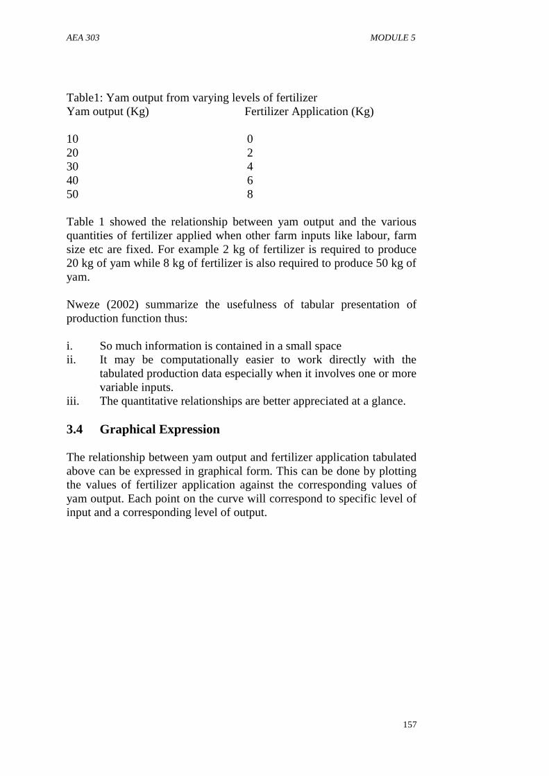
Table1: Yam output from varying levels of fertilizer
Yam output (Kg) Fertilizer Application (Kg)
10 0
20 2
30 4
40 6
50 8
Table 1 showed the relationship between yam output and the various
quantities of fertilizer applied when other farm inputs like labour, farm
size etc are fixed. For example 2 kg of fertilizer is required to produce
20 kg of yam while 8 kg of fertilizer is also required to produce 50 kg of
yam.
Nweze (2002) summarize the usefulness of tabular presentation of
production function thus:
i. So much information is contained in a small space
ii. It may be computationally easier to work directly with the
tabulated production data especially when it involves one or more
variable inputs.
iii. The quantitative relationships are better appreciated at a glance.
3.4 Graphical Expression
The relationship between yam output and fertilizer application tabulated
above can be expressed in graphical form. This can be done by plotting
the values of fertilizer application against the corresponding values of
yam output. Each point on the curve will correspond to specific level of
input and a corresponding level of output.

AEA 303 AGRICULTURAL PRODUCTION ECONOMICS
158
Fig 1: Typical production function
3.5 Mathematical Presentation
Mathematical expression is more explicit than ordinary functional
notation. There are many ways of expressing production function
mathematically. For example, production function can be expressed
explicitly in linear form as presented below:
Y = a + βx
Where
Y = quantity of output
X = quantity of input used
a = a constant
β = coefficient of X
If a and β takes on specific values like 10 and 0.5 respectively, the above
can then be expressed as follows:
Y = 10 + 0.5X
Unlike functional notation, this mathematical expression illustrated
above has the same content as in the graphical expression. It is however
more meaningful than the graphical approach because it allow one to
obtain the intermediate values of the variables.

AEA 303 MODULE 5
159
3.6 Written Word
The relationships between dependant and independent variables in
production function can be describe or enumerated in words without
resulting in to mathematical, graphical or tabular expression: this is a
very weak way of showing the relationship between two variables
because the magnitude of the relationship cannot be precisely stated by
ordinary word. Secondly, it will be difficult to comprehend the
statement at a glance. However, expression of production function in
word form is necessary to complement other forms of expression.
SELF-ASSESSMENT EXERCISE
Explain five ways of expressing production function
4.0 CONCLUSION
We discussed the various ways by which production function can be
expressed. The various ways identified in the unit include; written word,
tabular form, graphical form, symbolic form and mathematical form. We
can conclude here that combinations of these ways of expressing
production function are necessary to adequately specify the relationships
between two or more variables.
5.0 SUMMARY
The main points discussed in this unit are as follows:
(i) The following methods can be used to express production
function; written word, table, graph, mathematics and symbols.
(ii) Words expression is needed to complement other methods
(iii) In tabular form, we can quickly appreciate the relationship at a
glance
(iv) We can mathematically expressed the relationship as follows Y =
a + βx
(v) We can also use symbol like Y = ƒ (X1, X2, X3) to represent
relationship between Y and X in production function
(vi) We can also plot the graph of Y against X to express this
relationship.
(vii) We need combinations of these methods to satisfactorily explain
the relationship in production functions.
6.0 TUTOR-MARKED ASSIGNMENT

AEA 303 AGRICULTURAL PRODUCTION ECONOMICS
160
List and explain five ways of expressing production function.
7.0 REFERENCES/FURTHER READING
Abbot, J.C. and J.P. Makeham (1980). Agricultural Economics and
Marketing in the Tropics. London, Longman Publishers.
Adegeye, A.J. and J.S. Dittoh (1985). Essentials of Agricultural
Economics. Ibadan, Impact Publishers.
Nweze, N.J. (2002). Agricultural Production Economics: An
Introductory Text. Nsukka. AP Express Publishers.
Olayide, S.O. and Heady E.O. (1982). Introduction to Agricultural
Production Economics. Ibadan. University Press Ltd.
Olukosi, J.O. and A.O. Ogungbile (1989). Introduction to Agricultural
Production Economics: Principles and Applications. Zaria.
AGTAB Publishers Ltd.
Marshall A.C. (1998). Modern Farm Management Techniques. Owerri.
Alphabet Nigeria Publishers.
Reddy, S.S., P.R. Ram, T.V. Sastry and I.B. Devi (2004). Agricultural
Economics. New Delhi. Oxford and Ibh Publishers Ltd.

AEA 303 MODULE 5
161
UNIT 3 TYPES/FORMS OF PRODUCTION FUNCTION
CONTENTS
1.0 Introduction
2.0 Objectives
3.0 Main Content
3.1 Introduction
3.2 Linear Function
3.3 Quadratic Function
3.4 Cobb-Douglas Power Function
3.5 Square Root Function
3.6 Semi-Log Function
4.0 Conclusion
5.0 Summary
6.0 Tutor-Marked Assignment
7.0 References/Further Reading
1.0 INTRODUCTION
In the last unit we looked at the various ways we can express production
function. Some of the ways we discussed in that unit include: written
word, Table, Graph, Symbol and mathematics. We also discovered that
the use of combinations of these methods are necessary to adequately
describe the relationship between output and input. In this unit, we shall
go a step further to assess the various types of production functions used
in agricultural production economics. You are strongly advised to
carefully study this unit so that you can follow and understand the
subsequent units of this course.
2.0 OBJECTIVES
At the end of this unit, you should be able to:
identify and list the five major types of production function used
in agricultural production economics.
write the mathematical expression of these production functions
explain the application of at least three of these functions
state the major difference between these functions in agricultural
production economics.

AEA 303 AGRICULTURAL PRODUCTION ECONOMICS
162
3.0 MAIN CONTENTS
3.1 Introduction
In the estimation of production function parameters, many equation
forms have been fitted. Five of such equations that are commonly used
in agricultural production economics will be examine here. Those
examined include: linear, quadratic, Cobb-Douglas, square-root and
semi-log functions.
3.2 Linear Function
(a) Algebraic Form
The algebraic form of this equation can be expressed for the single
variables case as: Y = a + βX
Where Y = is the output and X is the variables input
a = intercept shown n the Y = axis, and
β = slope or gradient of the curve
The special features of linear function include
i. The curve is a straight line
ii. The slope of the curve must be constant
iii. The marginal product (MP) is also a straight horizontal line
(b) Marginal Product of Linear of Function
Y = a + bX………………….1
δY = b (MPP)……………….2
δX
(c) Elasticity of Production
If elasticity of production is given by this equation
∆Y . X …………………..3
∆X Y
Similarly, b which is the slope of the line gives the way in which
Y is changing for a unit change in the input X.
Therefore, if we make b the subject of equation 1, we then have
B = Y – a --------------4
X
Substituting b in equation 3, we have elasticity = (Y – a) × X
= (Y – a )……..5
X Y Y
From the above equation of elasticity we can deduce that:

AEA 303 MODULE 5
163

AEA 303 AGRICULTURAL PRODUCTION ECONOMICS
164
i. if a = 0, then elasticity = 1
ii. If a is greater than 0, then elasticity is less than 1
iii. if a is less than 0, then elasticity is greater than I
SELF-ASSESSMENT EXERCISE
Try the above equation with two variable inputs: Y = a + bx, + CX2
3.3 Quadratic Function
(a) Algebraic Form
For Single variables input we have:
Y = a + bX – Cx2
Where Y = output and X = variable input
a = the constant
b and c = the coefficients
Quadratic function allows diminishing total product. The coefficients of
X2 must have negative signs which implies diminishing marginal returns
(b) Marginal Product of Quadratic Function
Y = a + bx – cx2 ………………..6
δY = b – 2cx …………………..7
δX
Note that marginal product of quadratic function declines by a constant
absolute amount, secondly, marginal product curve is linear and thirdly,
quadratic function allows negative marginal product
(c) Elasticity in Quadratic Function
Ep = ∆y . X
∆x Y
Using equation 6 above we have
Ep = bx – 2cX2
a + bx – cX2
Note here that:
i. Elasticity in quadratic function declines with input magnitude
SELF-ASSESSMENT EXERCISE
AEA 303 MODULE 5
165
Find the marginal products and elasticities of quadratic function
involving two variable inputs: y = a + b1X1 + b2X2 – b3X12 – b4 X2
2 + b5
X1 X2
3.4 COBB – Douglas Power Function
(a) Algebraic Form
The single variable input of this function is presented as follows
Y = aXb
Where Y = output, X = variable input,
a = constant and b = elasticity of production
The Cobb – Douglas function is easy to estimate in its
logarithmic form. The above general form can be written in log
form as follows
log Y = log a + b log X
(b) Marginal Product
Y = aXb ……………….…9
δY = baXb – 1
(MPP) …….10
δX
Note:
i) Cobb-Douglas power function allows constant, increasing or
decreasing marginal productivity
ii) Cobb – Douglas allows any of the three above but not all the
three
iii) Marginal product declines if all other inputs are held constant.
(c) Elasticity of Production
Ep = ∆Y X ………………..11
∆X Y
∆Y in equation 10 = baXb- 1
….12
∆X
and Y = aXb
Substituting the two equations (12 and 13) in equation 11
We have
Ep = baXb . X = b……..………14
X aXb
Note the following features
i. The linearized log function of Cobb-Douglas power function is
easier to fit

AEA 303 AGRICULTURAL PRODUCTION ECONOMICS
166
ii. The coefficients of the function are the direct elasticities, i.e. the
partial elasticity are equal to each of the parameters
iii. When coefficient b = 1, we have a case of constant returns to
scale.
iv. When coefficient is greater than 1, we have a case of increasing
returns to scale
v. When coefficient is less than 1, we have a case of decreasing
returns to scale
Olukosi and Ogungbile (1989) identified some major shortcomings of
using this function as follows:
i. Cobb-Douglas function assumes a constant elasticity of
production over the entire output –input curve and therefore, the
function cannot be used for data which indicates both increasing
and decreasing marginal productivity.
ii. Similarly, it cannot be used for data with both positive and
negative marginal products
iii. It normally exhibits a non-linear relationship and it does not give
a defined maximum response at all input levels
SELF-ASSESSMENT EXERCISE
Find the marginal products and elasticities of this Cobb-Douglas power
function: Y = aX1b1
Xb2
2
3.5 Square Root Function
(a) Algebraic Form
A single variable algebraic form of square root function is
illustrated below:
Y = a + bX + cX0.5
Where Y = dependent variable (output), X = independent variable
(input), a = constant, b and c are the coefficients.
Just as in the case of quadratic function, square root function also
allows diminishing total product.
(b) Marginal Product
Y = a – bX + cX0.5
-----------------------------15
δY = -b + 0.5cX-0.5
(MPP)---------16
δX
The marginal product of this function declines at diminishing
rate.

AEA 303 MODULE 5
167

AEA 303 AGRICULTURAL PRODUCTION ECONOMICS
168
(c) Elasticity of Production
Y = a + bX + cX0.5
Ep = ΔY . X
ΔX Y
But ΔY in equation 16 = b + 0.5cX-0.5
ΔX
Therefore
Ep = 0.5cX-0.5
- b . X
Y
= [0.5cX-0.5
– b]X ----------------------17
Y
Elasticity in this function declines at high level of input and output. This
situation can happen under certain biological conditions.
SELF-ASSESSMENT EXERCISE
Determine the marginal products, elasticities and Rate of Products
Substitution for this function:
Y = a – b1X1 – b2X2 + b3X10.5
+ b4X20.5
+ b5X10.5
X20.5
3.6 Semi-Log Function
(a) Algebraic Function
Y = a + b log X
This function is very useful in aggregate production function analysis.
(b) Marginal Product
Y = a + b log X ………..18
δY = b (MPP)………..19
δX X
The marginal product declines with increase in variable input and vice
versa
(c) Elasticity of Production
Y = a + b log X
Ep = ∆Y . X
ΔX Y
From equation 19, MPP = b
X
EP = b . X = b ……………………….20
X Y Y
While marginal product varies with input, elasticity of production varies
with output.

AEA 303 MODULE 5
169
SELF-ASSESSMENT EXERCISE
Determine the MPP, RTS and EP for the Semi-log function of the two
variable inputs below:
Y = a + b1 logX1 + b2 logX2
4.0 CONCLUSION
In this unit we have examined five types of functional forms commonly
used in estimating parameters in agricultural production economics. The
functional forms examined include: linear function, quadratic function,
Cobb-Douglas power function, square-root function and Semi-log
function. We can conclude here that the choice of these functions will
depend on situation at hand.
5.0 SUMMARY
The main points in this unit include the followings:
i. Linear functions is of the form Y = a + bX for single input and Y
= a + bX1 + cX2 + dX3 for three variable inputs
ii. The algebraic form of quadratic function is Y = a + bX1 – cX12 +
dX2 – eX2
2 + fX3 – gX2
3 for three variable inputs
iii. Cobb – Douglas power function can be presented as Y =
aXb
1Xc2X3
d for three variable inputs
iv. Square root function can also be expressed as:
Y = a + bx1 + cX10.5
+ dX2+ eX20.5
fX3 + gX30.5
for three variable
inputs
v. Semi-log function can be expressed as follows Y = a + log X1+
b2 log X2 + b3 log X3 for three variables inputs
vi. Cobb- Douglas function can be linearized into logarithmic form
as follows:
Y = aX1bX
c2X
d3 linearized as Log Y = log a + b logX1 + c logX2
+ d logX3
6.0 TUTOR-MARKED ASSIGNMENT
1. List five types of production functions commonly used in
agricultural production economics
2. State their algebraic forms for two variable inputs
3. With examples, give full description of any three of them.

AEA 303 AGRICULTURAL PRODUCTION ECONOMICS
170
7.0 REFFERENCES/FURTHER READING
Abbot, J.C. and J.P. Makeham (1980). Agricultural Economics and
Marketing in the Tropics. London, Longman Publishers.
Adegeye, A.J. and J.S. Dittoh (1985). Essentials of Agricultural
Economics. Ibadan, Impact Publishers.
Nweze, N.J. (2002). Agricultural Production Economics: An
Introductory Text. Nsukka. AP Express Publishers.
Olayide, S.O. and Heady E.O. (1982). Introduction to Agricultural
Production Economics. Ibadan. University Press Ltd.
Olukosi, J.O. and A.O. Ogungbile (1989). Introduction to Agricultural
Production Economics: Principles and Applications. Zaria.
AGTAB Publishers Ltd.
Marshall A.C. (1998). Modern Farm Management Techniques. Owerri.
Alphabet Nigeria Publishers.
Reddy, S.S., P.R. Ram, T.V. Sastry and I.B. Devi (2004). Agricultural
Economics. New Delhi. Oxford and Ibh Publishers Ltd.

AEA 303 MODULE 5
171
UNIT 4 TIME PERIODS IN THE PRODUCTION
PROCESS
CONTENTS
1.0 Introduction
2.0 Objectives
3.0 Main Contents
3.1 Meaning
3.2 Short Run Production
3.3 Long Run Production Process
4.0 Conclusion
5.0 Summary
6.0 Tutor-Marked Assignment
7.0 References/Further Reading
1.0 INTRODUCTION
This unit 4 is the end of the units in module 2: in the last unit, we
discovered the various types of production functions commonly used in
agricultural production economics. These include: linear function,
quadratic function, Cobb-Douglas function, square-root function and
semi-log function. In this unit we shall go a step further to examine the
time periods in the production process.
2.0 OBJECTIVES
At the end of this unit, you should be able to explain the meaning of:
time periods in the production process
explain short run period of production
describe long run period of production
3.0 MAIN CONTENTS
3.1 Meaning
The time periods in the production process refers to the period of time
required for resources to adjust from its present status to new production
positions. In a production process, before a farmer can increase his
output, at least one of the resources must increase. Farm inputs like land,
labour and capital cannot increase at the same rate. Labour can be
adjusted quickly in response to increase demand for farm products, but
capital like building and farm equipment may take longer time. This

AEA 303 AGRICULTURAL PRODUCTION ECONOMICS
172
phenomena in the production process enables us to distinguish between
short run and long run production periods.
3.2 Short Run Period
The short run production period is defined as a period of time over
which at least one input can be varied while keeping other inputs fixed.
During this period farmer cannot increase or decrease their land and
capital resources.
However, some resources like labour can vary within short notice in
other to adjust to new level of output. Short run production period varies
according to the type of farm enterprise.
3.3 Long Run Period
The long run period of production process is defined as the period of
time long enough that all inputs can be varied. During this period of
time farm output can be increased with increase in all the farm inputs.
At this period of production process both farm size, farm building, farm
equipments can be varied.
The conditions for output and profit maximization in the short run
production process differ from that of long run period. In discussing
resource allocations, consideration must be given to the time period of
production process.
SELF-ASSESSMENT EXERCISE
Explain the time periods in production process
4.0 CONCLUSION
In this unit, we examined the meaning and types of time period of
production process. We identified two major types in the time period.
The short run and the long run period time in production. We can
conclude here, that the consideration of time is very important in output
and profit maximization.
5.0 SUMMARY
The main points in this unit include the followings:
i. Time period in the production process consider the period needed
for inputs to adjust to change in output.
AEA 303 MODULE 5
173
ii. The period that allow one input to vary while other inputs are
fixed is called short run period of production
iii. The period long enough for all factors of production to vary is
called long run period of production
iv. Time period in the production process is an important factor in
the determination of maximum output and profit.
6.0 TUTOR-MARKED ASSINGMENT
Explain with examples, the concept of short run and long run period of
time in the production process.
7.0 REFERENCES/FRUTHER READING
Abbot J. C and J.P Makeham (1980). Agricultural Economics and
marketing in the tropics London, Longman Publishers.
Adegeye A.J. and J.S Dittoh (1985) Essentials of Agricultural
Economics Ibandan, Impact Publishers.
Nweze N.J.(2002). Agricultural production Economics: An introduction
text Nsukka. AP Express Publishers.
Olayide S.O & Heady E.O (1982). Introduction to agricultural
Production Economics. Ibadan. University Press Ltd.
Olukosi J.O & A.O Ogungbile (1989). Introduction to Agricultural
Production Economics: Principles and Apllication Zaria. AGTAB
Publishers Ltd.
Marshall A.C (1998). Modern Farm Management Techniques. Owerri
Alphabet Nigeria Publishers.
Reddy S.S. P.R. Ram, T.V. Sastry and I.B. Devi (2004) Agricultural
Economic New Delhi. Oxford and Ibh Publishers Ltd.

AEA 303 AGRICULTURAL PRODUCTION ECONOMICS
174
MODULE 3 FACTOR – PRODUCT RELATIONSHIP
Unit 1 Laws of Returns
Unit 2 Classical Production Function
Unit 3 Output and Profit Maximization Under One Variable Input
Unit 4 Resource Allocation Involving More Than One Variable
Input
UNIT 1 LAWS OF RETURNS
CONTENTS
1.0 Introduction
2.0 Objectives
3.0 Main Contents
3.1 Introduction
3.2 Law of Increasing Returns
3.3 Law of Constant Returns
3.4 Law of Decreasing Returns
4.0 Conclusion
5.0 Summary
6.0 Tutor-Marked Assignment
7.0 References/Further Reading
1.0 INTRODUCTION
You are welcome to the first unit of Module 3. In Module 2, we
discussed the theory of production economics. In that module, we
discussed the meaning and uses of production function. Other things
discussed include: methods of expressing production function, types of
production function and time periods in the production process. In this
unit, we shall focus our attention on the laws of returns.
2.0 OBJECTIVES
At the end of this unit, you should be able to:
identify the three types of returns we have in production
relationships.
explain the laws of returns
use table, graph and mathematics to illustrate the three laws of
returns.

AEA 303 MODULE 5
175
3.0 MAIN CONTENTS
3.1 Introduction
In attempt to either maximize output or profit, farmers combine varying
levels of input factors in the production process. This various levels of
input usage by farmers allow the operations of the laws of returns.
The usefulness of this concept lies in its role as a classifying device. It
provides a convenient way of classifying particular types of
technological condition.
In a resource allocation involving one variable input factor while
keeping the other factors fixed, three different types of relationships can
be identified: increasing returns, constant returns and decreasing returns.
These relationships can be discussed using written words, tables, graphs
and mathematics.
3.2 Law Of Increasing Returns
Law of increasing returns is a situation in the production process in
which each successive unit of variable input adds more and more to the
output. That is, every addition to variable input adds more and more to
the output. In other words, every addition of variable input to the fixed
factors in the production process yield more to the total output than the
previous unit of output. This situation in the production process can also
be illustrated in a tabular form.
Table 2: Hypothetical Example of increasing Return
Variable Input Total Output Change in Input Change in Output
Marginal Return
X Y X Y
Y/ X
1 5 - -
-
2 10 1 5
5
3 20 1 10
10
4 35 1 15
15
5 55 1 20
20

AEA 303 AGRICULTURAL PRODUCTION ECONOMICS
176
From Table 2, addition of one unit of variable factor to 1 unit of input,
yielded marginal returns of 5. Addition of one unit to the second
variable factor yielded marginal returns of 10 and from 10 to 15 and 15
to marginal returns of 20. Every additions of one unit of variable factor
yielded more than the previous marginal returns.
This relationship can also be expressed graphically thus:
Fig. 2: Graphical Illustration of Increasing Returns
This relationship can also be expressed in mathematical form thus:
ΔY1 < ΔY2 < ΔY3 < ΔY4 < ΔY5
ΔX1 ΔX2 ΔX3 ΔX4 ΔX5
This shows that the marginal return in out Y1 and variable input X1 is
less than the marginal returns involving output Y2 and variable input X2
and so on.
3.3 Law of Constant Returns
The law of constant returns states that without varying the proportions in
which the factor of production area combined, there is an increase in
output proportionate to the increase in the total quantity of factors
employed. In other words, the addition of each successive unit of the
variable factor to the fixed factors adds the same to the output. For
example if all the quantities of all the inputs used in producing a given
TP
Ou
tpu
t (Y
)
Input (X)
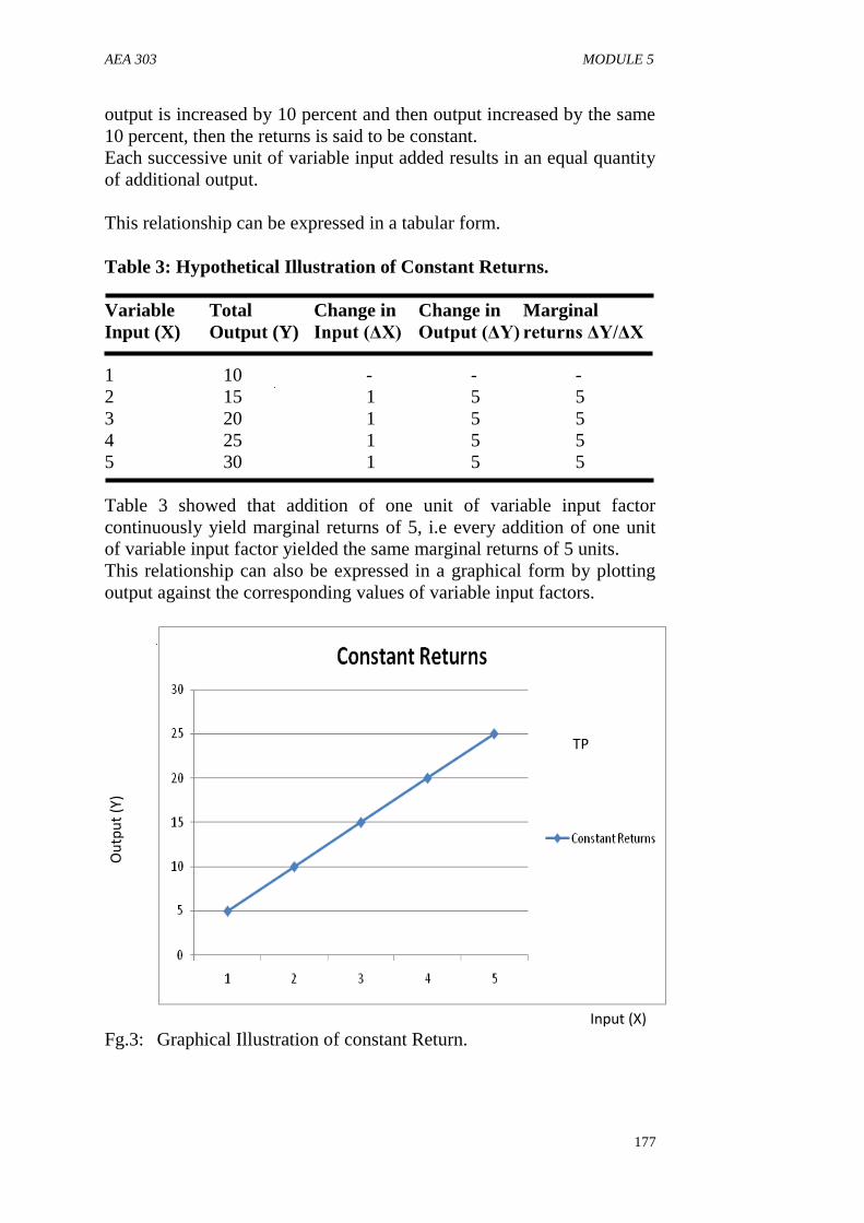
AEA 303 MODULE 5
177
output is increased by 10 percent and then output increased by the same
10 percent, then the returns is said to be constant.
Each successive unit of variable input added results in an equal quantity
of additional output.
This relationship can be expressed in a tabular form.
Table 3: Hypothetical Illustration of Constant Returns.
Variable Total Change in Change in Marginal
Input (X) Output (Y) Input (ΔX) Output (ΔY) returns ΔY/ΔX
1 10 - - -
2 15 1 5 5
3 20 1 5 5
4 25 1 5 5
5 30 1 5 5
Table 3 showed that addition of one unit of variable input factor
continuously yield marginal returns of 5, i.e every addition of one unit
of variable input factor yielded the same marginal returns of 5 units.
This relationship can also be expressed in a graphical form by plotting
output against the corresponding values of variable input factors.
Fg.3: Graphical Illustration of constant Return.
TP
Ou
tpu
t (Y
)
Input (X)

AEA 303 AGRICULTURAL PRODUCTION ECONOMICS
178
The graph showed a linear relationship producing a straight line curve.
The relationship can also be expressed in a mathematical form using
algebraic equation
ΔY1 = ΔY2 = ΔY3 = ΔY4 = ΔY5
ΔX1 ΔX2 ΔX3 ΔX4 ΔX5
This shows that the marginal returns in output Y1 and variable input X1
is exactly the same as in other relationships.
The condition of constant returns is unlikely to be met in agricultural
business.
3.4 Law of Decreasing Returns
The law of decreasing returns states that the addition of each successive
unit of the variable input to the fixed inputs in the production process,
adds less and less to the total output than the previous unit.
Alternatively, it can be stated that for each addition to the variable factor
the addition to the total output declines. This law can further be
illustrated thus: suppose that the quantities of all the inputs used in
producing a given output are increased for example by 10 percent and if
output increases by smaller proportion e.g a percent or less, then return
to scale is said to be decreasing. Decreasing returns can also be
expressed in a tabular form
Table 4: Hypothetical Illustration of Decreasing Returns
Variable Total Change in Change in Marginal Returns
Input (X) output (Y) input ( X) Output ( Y) Y/X
1 10 - - -
2 35 1 25 25
3 45 1 20 20
4 60 1 15 15
5 70 1 10 10
From Table 4, addition of 1 unit of X to the initial unit of X, yielded
marginal returns of 25 units. Addition of 1 unit of X to the second
variable input yielded less marginal returns of 20. Every subsequent
additions of one unit of variable factors yielded less than the previous
marginal returns.
This relationship can equally be represented in a graphical form.

AEA 303 MODULE 5
179
Fig. 4: Graphical Representation of Decreasing Returns
The graph depicts a concave relationship to the x-axis. We can also
express this relationship between variable input factor and output in
algebra form as follows:
ΔY1 > ΔY2 > ΔY3 > ΔY4 > ΔY5
ΔX1 ΔX2 ΔX3 ΔX4 ΔX5
Mathematically, this relationship shows that the marginal returns in
output Y1 and variable input X1 is more than the marginal returns
involving output Y2 and input X2 and son on.
SELF-ASSESSMENT EXERCISE
List and explain the three types of returns in production relationships
4.0 CONCLUSION
This unit focused on the laws of returns. In this unit we identified three
major types of returns in production process. These returns can be
increasing, constant or decreasing. Knowledge of these relationships is
very important in agricultural production because it provides a
convenient way of classifying particular types of technological
condition.
TP
Input (X)
Ou
tpu
t (Y
)
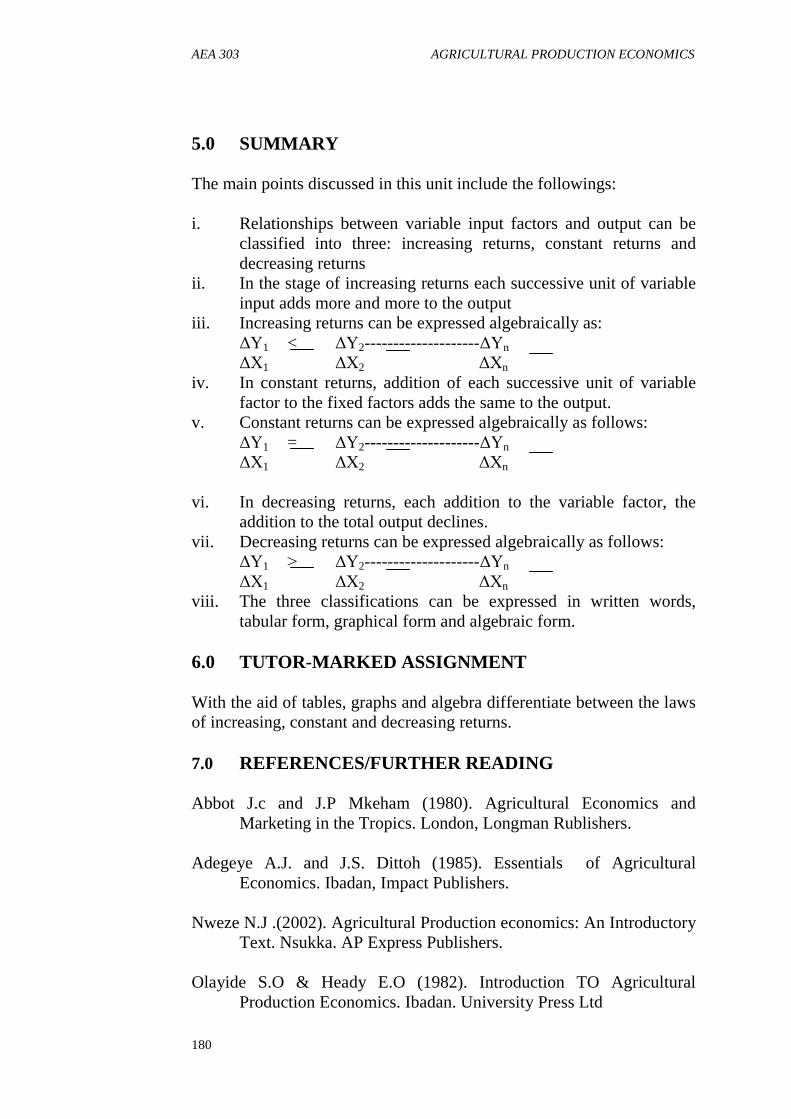
AEA 303 AGRICULTURAL PRODUCTION ECONOMICS
180
5.0 SUMMARY
The main points discussed in this unit include the followings:
i. Relationships between variable input factors and output can be
classified into three: increasing returns, constant returns and
decreasing returns
ii. In the stage of increasing returns each successive unit of variable
input adds more and more to the output
iii. Increasing returns can be expressed algebraically as:
ΔY1 < ΔY2--------------------ΔYn
ΔX1 ΔX2 ΔXn
iv. In constant returns, addition of each successive unit of variable
factor to the fixed factors adds the same to the output.
v. Constant returns can be expressed algebraically as follows:
ΔY1 = ΔY2--------------------ΔYn
ΔX1 ΔX2 ΔXn
vi. In decreasing returns, each addition to the variable factor, the
addition to the total output declines.
vii. Decreasing returns can be expressed algebraically as follows:
ΔY1 ˃ ΔY2--------------------ΔYn
ΔX1 ΔX2 ΔXn
viii. The three classifications can be expressed in written words,
tabular form, graphical form and algebraic form.
6.0 TUTOR-MARKED ASSIGNMENT
With the aid of tables, graphs and algebra differentiate between the laws
of increasing, constant and decreasing returns.
7.0 REFERENCES/FURTHER READING
Abbot J.c and J.P Mkeham (1980). Agricultural Economics and
Marketing in the Tropics. London, Longman Rublishers.
Adegeye A.J. and J.S. Dittoh (1985). Essentials of Agricultural
Economics. Ibadan, Impact Publishers.
Nweze N.J .(2002). Agricultural Production economics: An Introductory
Text. Nsukka. AP Express Publishers.
Olayide S.O & Heady E.O (1982). Introduction TO Agricultural
Production Economics. Ibadan. University Press Ltd

AEA 303 MODULE 5
181
Olukosi J.O & A.O Ogungbrle (1989). Introduction to Agricultural
Production Economics: principles and Applications Zaria
AGTAB Publishers Ltd.
Marshall A.C. (1998). MODERN Farm Management Techniques.
Owerri Alphabet Nigeria Publishers
Reddy S.S., P.R. Ram, T.V. Sastry and I.B. Devi (2004). Agricultural
Economics New Dlhi. Oxford and Ibh Publilshers Ltd.

AEA 303 AGRICULTURAL PRODUCTION ECONOMICS
182
UNIT 2 CLASSICAL PRODUCTION FUNCTION
CONTENTS
1.0 Introduction
2.0 Objectives
3.0 Main Contents
3.1 Relationship Between TPP, APP and MPP
3.2 Law of Diminishing Returns
3.3 Stages of Production Function
3.4 Reasons for Increasing, Decreasing and Negative Returns
4.0 Conclusion
5.0 Summary
6.0 Tutor-Marked Assignment
7.0 References/Further Reading
1.0 INTRODUCTION
In unit 1 of this module, we discussed the laws of returns. We classified
return to scale in production process into three – increasing returns,
constant returns and decreasing returns. We differentiated these three
stages through written words, tabular form, graphical form and algebraic
form. In this unit 2, we shall go a step further to look at classical
production function in a case of one variable input.
Under the classical production function we shall discuss the relationship
between Total Physical Product (TPP), Average Physical Product (APP)
and Marginal Physical Product (MPP). We shall also use these
relationships to establish the law of diminishing returns and classify
production function into three stages.
2.0 OBJECTIVES
At the end of this unit, you should be able to:
explain the meaning of total physical product, average physical
product and marginal physical product.
plot the graph of a classical production function
establish the relationship between TPP and APP, TPP and MPP
and APP and MPP.
explain the law of diminishing returns
differentiate the three stages of production function
give one reason for increasing, decreasing and negative returns.
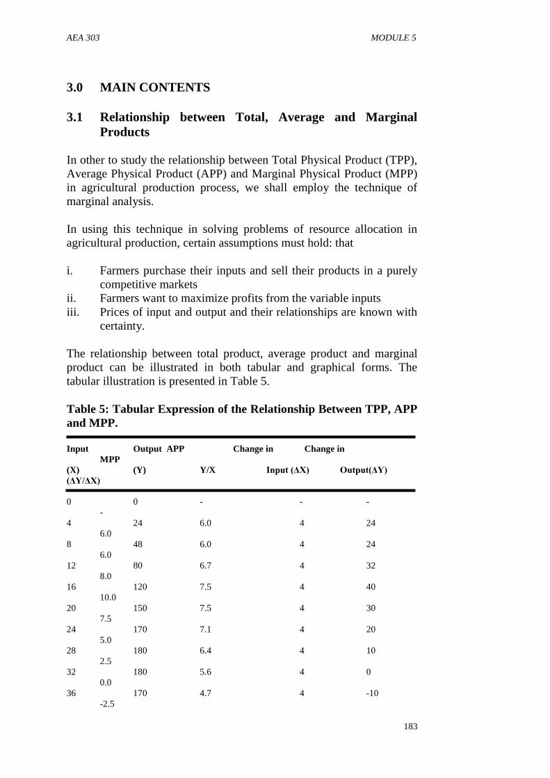
AEA 303 MODULE 5
183
3.0 MAIN CONTENTS
3.1 Relationship between Total, Average and Marginal
Products
In other to study the relationship between Total Physical Product (TPP),
Average Physical Product (APP) and Marginal Physical Product (MPP)
in agricultural production process, we shall employ the technique of
marginal analysis.
In using this technique in solving problems of resource allocation in
agricultural production, certain assumptions must hold: that
i. Farmers purchase their inputs and sell their products in a purely
competitive markets
ii. Farmers want to maximize profits from the variable inputs
iii. Prices of input and output and their relationships are known with
certainty.
The relationship between total product, average product and marginal
product can be illustrated in both tabular and graphical forms. The
tabular illustration is presented in Table 5.
Table 5: Tabular Expression of the Relationship Between TPP, APP
and MPP.
Input Output APP Change in Change in
MPP
(X) (Y) Y/X Input (ΔX) Output(ΔY)
(ΔY/ΔX)
0 0 - - -
-
4 24 6.0 4 24
6.0
8 48 6.0 4 24
6.0
12 80 6.7 4 32
8.0
16 120 7.5 4 40
10.0
20 150 7.5 4 30
7.5
24 170 7.1 4 20
5.0
28 180 6.4 4 10
2.5
32 180 5.6 4 0
0.0
36 170 4.7 4 -10
-2.5
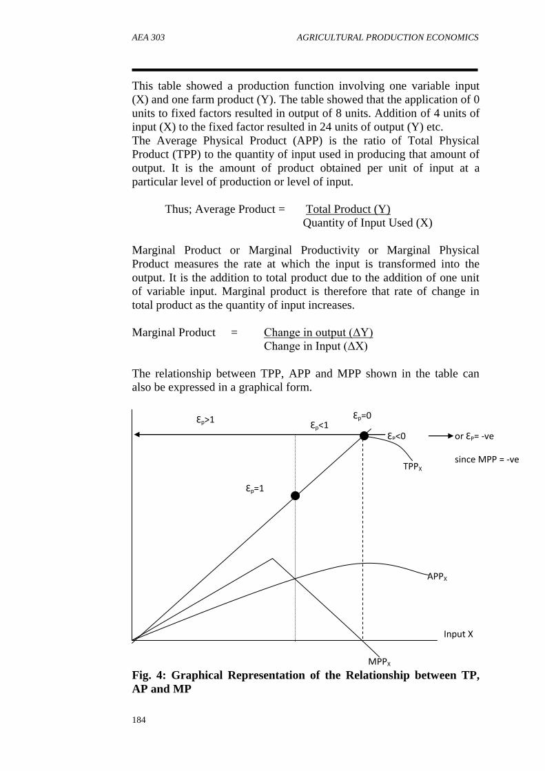
AEA 303 AGRICULTURAL PRODUCTION ECONOMICS
184
This table showed a production function involving one variable input
(X) and one farm product (Y). The table showed that the application of 0
units to fixed factors resulted in output of 8 units. Addition of 4 units of
input (X) to the fixed factor resulted in 24 units of output (Y) etc.
The Average Physical Product (APP) is the ratio of Total Physical
Product (TPP) to the quantity of input used in producing that amount of
output. It is the amount of product obtained per unit of input at a
particular level of production or level of input.
Thus; Average Product = Total Product (Y)
Quantity of Input Used (X)
Marginal Product or Marginal Productivity or Marginal Physical
Product measures the rate at which the input is transformed into the
output. It is the addition to total product due to the addition of one unit
of variable input. Marginal product is therefore that rate of change in
total product as the quantity of input increases.
Marginal Product = Change in output (ΔY)
Change in Input (ΔX)
The relationship between TPP, APP and MPP shown in the table can
also be expressed in a graphical form.
Fig. 4: Graphical Representation of the Relationship between TP,
AP and MP
Ɛp=1
ƐP<0
MPPX
Input X
APPX
Ɛp<1 Ɛp>1 Ɛp=0
TPPX
or ƐP= -ve
since MPP = -ve
AEA 303 MODULE 5
185
Table 5 and Fig. 4 will give us a clearer understanding on the
relationship between production function variables (TP, AP and MP).
We can divide these relationships into three categories:
i. Relationship between TPP and APP
From fig. 4, we can see that APP curve is similar in shape to TPP, this is
because APP is purely derived from TPP.
Where TPP is increasing at an increasing rate, APP curve is also
increasing.
ii. Relationship between TPP and MPP
When TPP curve is increasing at an increasing rate, the MPP
curve is also increasing.
When TPP curve is increasing at a decreasing rate, the MPP
curve is decreasing.
The point at which MPP is at its maximum corresponds to the
inflection point on the TPP curve.
Beyond the inflection point, TPP continues to increase at a
decreasing rate but MPP begins to decrease.
Where TPP reaches its peak and has zero slope, MPP becomes
zero.
At the point where TPP curve begins to decline (point of
intensive margin), MPP is negative.
iii. The relationship between MPP and APP
When APP is increasing, MPP curve is above APP curve [MPP >
APP].
When APP is decreasing, MPP curve is below the APP curve
[MPP<APP]
Where APP curve is at its peak, both APP and MPP are equal
(MPP = APP)
Where MPP curve is zero, APP curve is still decreasing but
positive.
At the point where MPP is negative, APP curve is decreasing but
still positive.
SELF-ASSESSMENT EXERCISE
Complete the table by calculating the Average Product and Marginal
Product.

AEA 303 AGRICULTURAL PRODUCTION ECONOMICS
186
Variable Unit Fixed Factor Total Product Average Marginal
Of Labour (Land) (Kg) Product (kg) Product
(kg)
1 3 8
2 3 18
3 3 36
4 3 48
5 3 55
6 3 60
7 3 60
8 3 56
3.2 Law of Deminishing Returns
Diminishing returns is the most observed phenomena in production for
most inputs especially at normal production levels. The law of
diminishing returns states that if the quantity of one variable factor is
increased by equal amount while the quantity of other factors are kept
constant, the marginal product and average product of the variable factor
will eventually decrease. According to Olukosi and Ogungbile (1989),
law of diminishing returns can be stated in terms of the TPP, APP and
MPP.
In terms of TPP, the law states that “Given a set of fixed input, if we
apply successive equal increments of a variable input, the total physical
output first increases at an increasing rate, then increases at a decreasing
rate, reaches a maximum and then declines”.
In terms of APP, the law states that “Given a set of fixed inputs, if we
apply successive equal increments of a variable input, the APP
increases, reaches a maximum (when it equals to MPP) and decreases
henceforth”.
When stated in terms of MPP, the law states that “Given a set of fixed
inputs, if we apply successive equal increments of a variable input, the
MPP first increases, reaches a maximum, decreases to zero and then
become negative”. It is therefore important when stating this law to
specify whether it is in terms of TPP; APP or MPP. The law is also
called law of variable proportions because various amounts of the
variable inputs are applied to a fixed quantity of input factors.
This law is important because it enables us to identify the right amount
of variable input to be combined with the fixed input. The fixed factors
like farm size imposes a limit to the amount of additional output that can

AEA 303 MODULE 5
187
be obtained from the addition of more variable input. This implies that
the law cannot stand if there is no fixed factor in the production process.
3.3 Stages of Production Function
A typical production function such as the type illustrated in Table 5 and
Fig 4 can be divided into three distinct stages. Fig. 4 showing TPP, APP
and MPP curves can be reproduced to show the three stages in
production process.
Fig. 5: Illustration of the Three Stages of Production
Characteristic Features of Stage 1
Stage 1 ends with the extensive margin where APP equals MPP
TPP first increases at an increasing rate and then from the point
of inflection begins to increase at a decreasing rate.
MPP increases and reaches a peak and begins to decline.
APP also continues to increase and reaches its peak where stage 1
terminates.
At this stage MPP is greater than APP
The average rate at which input X is being converted to output is
still increasing.
Stage
1
Stage
11
Stage
111
MPPX
Input X
APPX
Ɛp<1 Ɛp>1 Ɛp=0
Ɛp=1
TPPX
ƐP<0 or ƐP= -ve
since MPP = -ve

AEA 303 AGRICULTURAL PRODUCTION ECONOMICS
188
In this stage, it is advisable for farmers to continue to add more
variable input.
It is an irrational stage of production
All the input resources are increasing.
The technical efficiency of variable input decreases as indicated
by the decrease in APP.
The technical efficiency of fixed inputs increases as indicated by
increase in TPP.
Characteristic Features of Stage 2
Stage 2 of production starts where APP is equal to MPP.
After this point APP is greater than MPP
At the end of stage 2 MPP is equal to zero
In stage 2, MPP is equal to or less than APP but equal to or
greater than zero.
This stage represents the region of rational production where
profit could be maximized.
Elasticity of production is less than one, but equal to zero at the
end of the stage.
Characteristic Features of Stage 3
Stage 3 of production starts where MPP is equal to zero
In stage 3, MPP becomes negative
Both TPP and APP continue to decrease
Elasticity of production is less than zero
Variable resource is in excess relative to fixed resources.
The technical efficiency of variable resource and fixed resources
declines
Stage 3 is therefore irrational stage of production
Summary of Three Stages of Production Function:
S.No. Stage 1 Stage II Stage III
1. Starts from the origin Starts from where Starts from where And ends where APP is maximum MPP is zero or TPP
MPP = APP and ends where MPP is maximum.
is zero.
2. TPP increases at TPP increase at TPP decreases at
Increasing rate decreasing rate increasing rate up to the point
of reflection.
3. MPP > APP MPP < APP -
The characteristic features of these three stages of production showed
that stage 2 should be the area of operation for a rational farmer. In stage

AEA 303 MODULE 5
189
2, the ratio of the variable resource to fixed resources is higher to the
extent that adjustment between the two extremes is possible. Based on
physical considerations, production is limited to stage 2. However, the
determination of the exact point of maximum net revenue required
additional information of the prices of input and output.
3.4 Reasons for Increasing, Decreasing and Negative Returns
Reddy et al (2004) gave reasons for the observation of increasing,
decreasing and negative returns in production process as follows:
In stage 1, the surplus fixed inputs are not put to efficient utilization due
to insufficient availability of variable input. Under this situation
application of more quantities of variable input makes the excess fixed
input relative to variable input to be more efficiently utilized. This
situation leads to increasing returns. As we continue to apply more of
the variable input to fixed input a time will come when we reach
maximum marginal physical product. Beyond this point any further
addition of variable input to fixed inputs will result into less addition to
output. This is the point of decreasing returns.
As we noticed the situation of decreasing returns, if more and more of
variable input is added to the fixed factors, the variable resource
becomes too large to fixed resources. At this stage the unused variable
resource will impede production process instead of enhancing it. This
leads to the situation of negative returns.
4.0 CONCLUSION
In this unit, we discussed the relationship between total, average and
marginal physical products in a production function. We used that
relationship to establish the law of diminishing returns as well as
classifying production process into three stages. We finally in this unit
give reasons why we observed increasing, decreasing and negative
returns in a production process. The interaction between the concepts of
TPP, APP and MPP made us to identify the rational and irrational
regions of production.
5.0 SUMMARY
The main points in this unit include the followings:
i. There are assumptions that underlie the use of the technique of
marginal analysis in resource allocation.
ii. APP = TPP (Y)
AEA 303 AGRICULTURAL PRODUCTION ECONOMICS
190
Input Used (X)
iii. MPP = Change in TPP (ΔY)
Change in Input (ΔX)
iv. The relationship between TPP, APP and MPP can be expressed
both in tabular and graphical form
v. APP and MPP curves are similar in shape to TPP because both of
them are produced from TPP.
vi. Law of diminishing returns can be defined from the perspective
of TPP, APP and MPP.
vii. Three stages or regions can be identified in production process.
viii. Stages 1 and 3 represent irrational regions in the production
process because maximum net return can never be achieved in
the two regions.
ix. Stage 2 represents the rational region of production where we can
obtain maximum profit.
x. Availability of both variable and fixed inputs in resource
allocation will determine whether a production process will
operates increasing, decreasing or negative returns.
6.0 TUTOR-MARKED ASSIGNMENT
1. Explain the meaning of the following concepts in production
function:
(a) Average Physical Product (APP)
(b) Marginal Physical Product (MPP)
(c) Law of diminishing returns
(d) Rational Production Stage
(e) Irrational Production
7.0 REFERENCES/FURTHER READING
Abbot J.c and J.P Mkeham (1980). Agricultural Economics and
Marketing in the Tropics. London, Longman Rublishers.
Adegeye A.J. and J.S. Dittoh (1985). Essentials of Agricultural
Economics. Ibadan, Impact Publishers.
Nweze N.J .(2002). Agricultural Production economics: An Introductory
Text. Nsukka. AP Express Publishers.
Olayide S.O & Heady E.O (1982). Introduction TO Agricultural
Production Economics. Ibadan. University Press Ltd
AEA 303 MODULE 5
191
Olukosi J.O & A.O Ogungbrle (1989). Introduction to Agricultural
Production Economics: principles and Applications Zaria
AGTAB Publishers Ltd.
Marshall A.C. (1998). MODERN Farm Management Techniques.
Owerri Alphabet Nigeria Publishers
Reddy S.S., P.R. Ram, T.V. Sastry and I.B. Devi (2004). Agricultural
Economics New Dlhi. Oxford and Ibh Publilshers Ltd.

AEA 303 AGRICULTURAL PRODUCTION ECONOMICS
192
UNIT 3 OUTPUT AND PROFIT MAXIMIZATION
UNDER ONE VARIABLE INPUT
CONTENTS
1.0 Introduction
2.0 Objectives
3.0 Main contents
3.1 Determination of optimum output
3.2 Determination of optimum profit
3.3 Input Demand Curve
3.4 Elasticity of production
4.0 Conclusion
5.0 Summary
6.0 Tutor-Marked Assignment
7.0 References/Further Reading
1.0 INTRODUCTION
You are welcome to another unit under module 3. In unit 2, we
discussed the classical production function. Under the unit, we explained
the relationship between TPP, APP and MPP in a production function.
We further used this relationship to establish the law of diminishing
returns. We also used that relationship to categorized production process
into three stages, we identified the distinguishing features of each stage.
We then proceeded to find reasons for increasing, decreasing and
negative returns in production process. In this unit we shall focus
our attention on output and profit maximization involving variable input.
2.0 OBJECTIVES
At the end of this unit, you should be able to:
i. explain how optimum output is determined
ii. describe how optimum profit is determined using production
function approach
iii. formulate the determination of optimum profit using profit
function approach.
iv. explain how input demand curve is obtained from production
function
v. formulate output elasticity
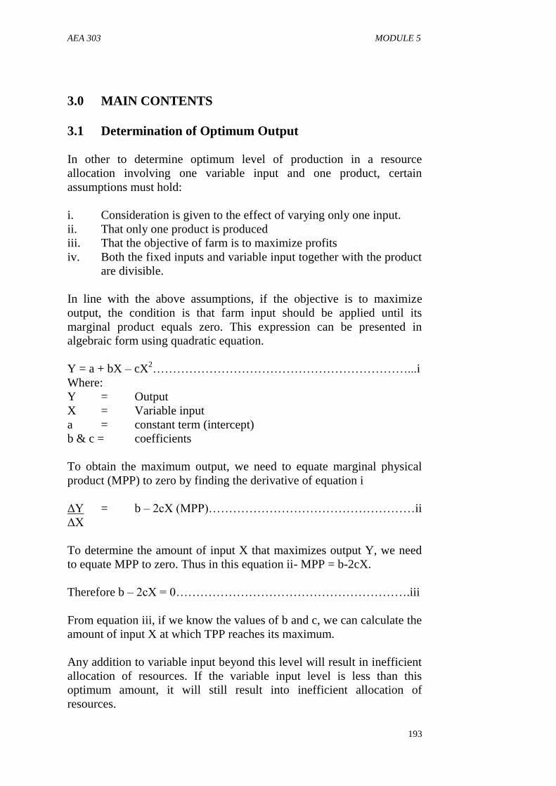
AEA 303 MODULE 5
193
3.0 MAIN CONTENTS
3.1 Determination of Optimum Output
In other to determine optimum level of production in a resource
allocation involving one variable input and one product, certain
assumptions must hold:
i. Consideration is given to the effect of varying only one input.
ii. That only one product is produced
iii. That the objective of farm is to maximize profits
iv. Both the fixed inputs and variable input together with the product
are divisible.
In line with the above assumptions, if the objective is to maximize
output, the condition is that farm input should be applied until its
marginal product equals zero. This expression can be presented in
algebraic form using quadratic equation.
Y = a + bX – cX2………………………………………………………...i
Where:
Y = Output
X = Variable input
a = constant term (intercept)
b & c = coefficients
To obtain the maximum output, we need to equate marginal physical
product (MPP) to zero by finding the derivative of equation i
ΔY = b – 2cX (MPP)……………………………………………ii
ΔX
To determine the amount of input X that maximizes output Y, we need
to equate MPP to zero. Thus in this equation ii- MPP = b-2cX.
Therefore b – 2cX = 0………………………………………………….iii
From equation iii, if we know the values of b and c, we can calculate the
amount of input X at which TPP reaches its maximum.
Any addition to variable input beyond this level will result in inefficient
allocation of resources. If the variable input level is less than this
optimum amount, it will still result into inefficient allocation of
resources.

AEA 303 AGRICULTURAL PRODUCTION ECONOMICS
194
Therefore, maximum output under this condition is the highest amount
of output that could be technically produced. It is the highest feasible
output and does not consider the prices of input and output in its
computation. That is why the value of optimum output is usually higher
than the economic optimum output.
Working Example
1. Consider the production function of maize output as follows: Y =
100 + 400X – 2X2
Where Y = maize output (kg) and X = fertilizer application (kg)
Calculate: (a) the level of input that will maximize maize output.
(b) The optimum quantity of maize that could be
produced.
Solution to the problem
(a) Consider the equation: Y = 100 + 400X – 2X2
Optimum level is achieved when MPP = 0
Therefore Y = 400 – 4X = 0
X
4X = 400 and X = 400 = 100
4
Answer = The level of input that will maximize maize Output = 100kg
of fertilizer
(b) Optimum quantity of maize that could be produced
This can be obtained by substituting the value of input X into the
formula
Y = 100 + 400X – 2X2
= 100 + 400(100) – 2(100) 2
= 100 + 40,000 – 2(10,000)
= 40,100 – 20,000 = 20,100kg
Optimum Output of maize produced = 20,100kg
SELF-ASSESSMENT EXERCISE
1. Find the level of input and the optimum product that could be
produced from the production function below:

AEA 303 MODULE 5
195
Q = 300 X – 2X3
3.2 Determination of Optimum Profit
In a factor – product relationship involving one variable input and one
product, if the objective is to maximize profit (i.e economic optimum),
then prices of the input and output in addition to the quantities of input
and output are required.
We can approach profit maximization through any of the following
methods:
(a) Production function Approach
(b) Total Profit function Approach
a. Production Function Approach
Note that the condition for profit maximization under one variable input
requires that input be applied until the value of its marginal product is
equal to the price of the input i.e. VMPx = Px…………………………iii
Consider the following: Let
Px = Price of input
Py = Price of output
X = Change in input
Y = Change in output
PX ΔX = Additional unit cost of input
Py ΔY = Additional unit value of output
From equation III, MPx = ΔY and V = Py
ΔX
Therefore VMPx = Py ( ΔY)
ΔX
At optimum profit VMPx = Px
Py . (ΔY) = Px ……………………………………….iv
ΔX
Where
Py = Price of output Y
Px = Price of input X
ΔY = Marginal product of X
ΔX
We can rewrite equation iv thus:
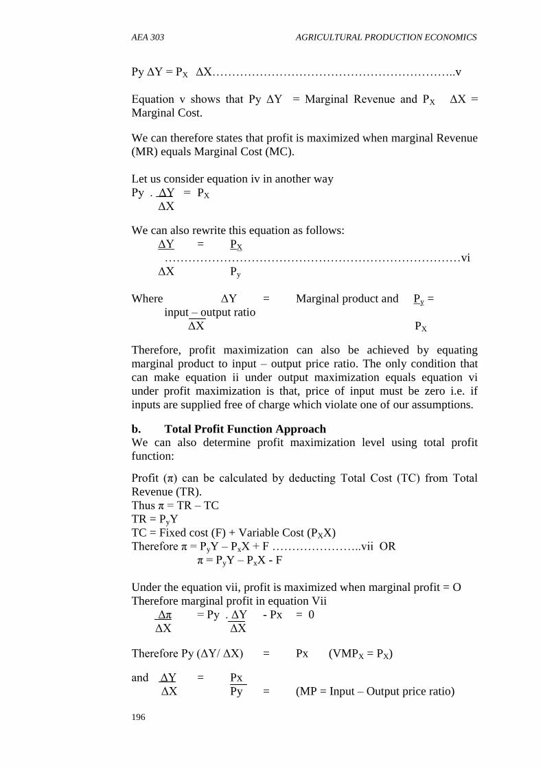
AEA 303 AGRICULTURAL PRODUCTION ECONOMICS
196
Py ΔY = PX ΔX……………………………………………………..v
Equation v shows that Py ΔY = Marginal Revenue and PX ΔX =
Marginal Cost.
We can therefore states that profit is maximized when marginal Revenue
(MR) equals Marginal Cost (MC).
Let us consider equation iv in another way
Py . ΔY = PX
ΔX
We can also rewrite this equation as follows:
ΔY = PX
…………………………………………………………………vi
ΔX Py
Where ΔY = Marginal product and Py =
input – output ratio
ΔX PX Therefore, profit maximization can also be achieved by equating
marginal product to input – output price ratio. The only condition that
can make equation ii under output maximization equals equation vi
under profit maximization is that, price of input must be zero i.e. if
inputs are supplied free of charge which violate one of our assumptions.
b. Total Profit Function Approach
We can also determine profit maximization level using total profit
function:
Profit (π) can be calculated by deducting Total Cost (TC) from Total
Revenue (TR).
Thus π = TR – TC
TR = PyY
TC = Fixed cost (F) + Variable Cost (PXX)
Therefore π = PyY – PxX + F …………………..vii OR
π = PyY – PxX - F
Under the equation vii, profit is maximized when marginal profit = O
Therefore marginal profit in equation Vii
Δπ = Py . ΔY - Px = 0
ΔX ΔX
Therefore Py (ΔY/ ΔX) = Px (VMPX = PX)
and ΔY = Px
ΔX Py = (MP = Input – Output price ratio)

AEA 303 MODULE 5
197
Or Py ΔY = Px ΔX = (Marginal Revenue = Marginal Cost)
All these indicate the best point to produce. Profit maximization level is
the point where the use of additional input yield exactly the same
amount of additional return. At this point it neither pays to increase nor
decrease the use of the input in production.
3.3 Input Demand Curve
We have already discovered that the rational stage of production where
profit can be maximized is stage 2. In this stage, we noticed a downward
sloping of marginal product. Between the beginning and end of stage 2,
we can derive an input demand curve for the purpose of determining an
optimum input level that will maximize profit.
The condition for profit maximization is that the value of marginal
product should be equal to the input price i.e. VMPx = Px. Fig.6 showed
VMPx on the vertical line and X on the horizontal line. The implication
of this relationship is that where VMPx meet X on the input demand
curve, profit is maximized.
From fig. 6, when the input price is Px, then the input quantity that will
be required to maximize profit is X1 (point A). Similarly, if the input
price is reduced to PX2, the quantity of input X required to maximize
profit will be X2 (point B). We can therefore say that input demand is
the quantity of input X that a farmer will require to maximize profit.
VMPx
Input X
A
B
Px1
Px2
X1 X2
Fig. 7: Derived Demand Curve for profit-maximizing input level
0
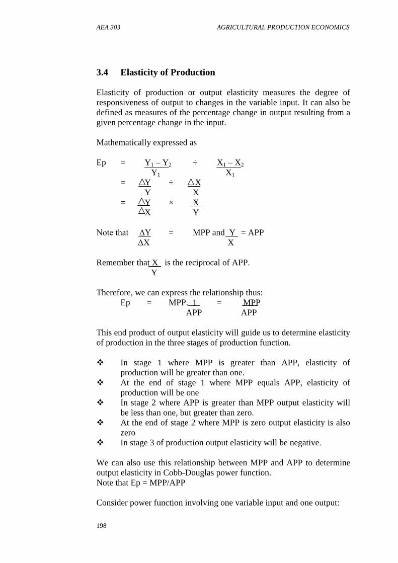
AEA 303 AGRICULTURAL PRODUCTION ECONOMICS
198
3.4 Elasticity of Production
Elasticity of production or output elasticity measures the degree of
responsiveness of output to changes in the variable input. It can also be
defined as measures of the percentage change in output resulting from a
given percentage change in the input.
Mathematically expressed as
Ep = Y1 – Y2 ÷ X1 – X2
Y1 X1
= Y ÷ X
Y X
= Y × X
X Y
Note that ΔY = MPP and Y = APP
ΔX X
Remember that X is the reciprocal of APP.
Y
Therefore, we can express the relationship thus:
Ep = MPP. 1 = MPP
APP APP
This end product of output elasticity will guide us to determine elasticity
of production in the three stages of production function.
In stage 1 where MPP is greater than APP, elasticity of
production will be greater than one.
At the end of stage 1 where MPP equals APP, elasticity of
production will be one
In stage 2 where APP is greater than MPP output elasticity will
be less than one, but greater than zero.
At the end of stage 2 where MPP is zero output elasticity is also
zero
In stage 3 of production output elasticity will be negative.
We can also use this relationship between MPP and APP to determine
output elasticity in Cobb-Douglas power function.
Note that Ep = MPP/APP
Consider power function involving one variable input and one output:
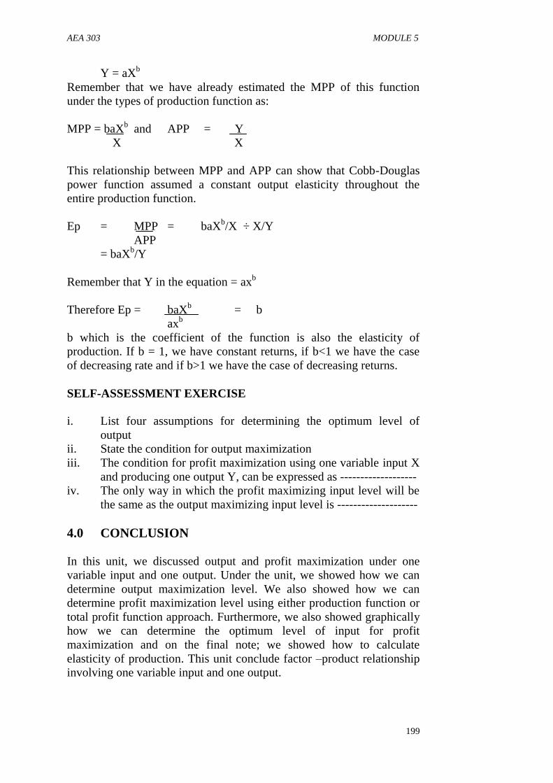
AEA 303 MODULE 5
199
Y = aXb
Remember that we have already estimated the MPP of this function
under the types of production function as:
MPP = baXb
and APP = Y
X X
This relationship between MPP and APP can show that Cobb-Douglas
power function assumed a constant output elasticity throughout the
entire production function.
Ep = MPP = baXb/X ÷ X/Y
APP
= baXb/Y
Remember that Y in the equation = axb
Therefore Ep = baXb = b
axb
b which is the coefficient of the function is also the elasticity of
production. If b = 1, we have constant returns, if b<1 we have the case
of decreasing rate and if b>1 we have the case of decreasing returns.
SELF-ASSESSMENT EXERCISE
i. List four assumptions for determining the optimum level of
output
ii. State the condition for output maximization
iii. The condition for profit maximization using one variable input X
and producing one output Y, can be expressed as -------------------
iv. The only way in which the profit maximizing input level will be
the same as the output maximizing input level is --------------------
4.0 CONCLUSION
In this unit, we discussed output and profit maximization under one
variable input and one output. Under the unit, we showed how we can
determine output maximization level. We also showed how we can
determine profit maximization level using either production function or
total profit function approach. Furthermore, we also showed graphically
how we can determine the optimum level of input for profit
maximization and on the final note; we showed how to calculate
elasticity of production. This unit conclude factor –product relationship
involving one variable input and one output.

AEA 303 AGRICULTURAL PRODUCTION ECONOMICS
200
5.0 SUMMARY
The main points in this unit include the followings:
i. To determine optimum levels of output and profit, certain
assumptions must hold.
ii. Output maximization requires that input be applied until MPP
equals zero (MPP = 0)
iii. Profit maximization condition requires that input be applied until
MPP is equal to the price of the input (VMPx = Px).
iv. The condition that can make the objectives of output and profit
maximization equal is when input price is free (Px = 0)
v. We can use production function or total profit function to
determine optimum profit
vi. We can use the downward slope of MPP in stage 2 of production
function to determine the optimum input level that will maximize
profit and this approach is called input demand curve
vii. Output elasticity or elasticity of production measures the degree
of responsiveness of output to changes in the variable input.
viii. Output elasticity varies as we move along the slope of production
function.
ix. Output elasticity in Cobb-Douglas power function is the same
with the values of its coefficients.
6.0 TUTOR-MARKED ASSIGNMENT
Consider the production function of a farmer below:
Y = 10 + 200X – 2X2 and the price of input = N10 and price of output =
N 50.
Calculate the optimum profit and output of this function.
7.0 REFERENCES/FURTHER READING
Abbot, J.C. and J.P. Makeham (1980). Agricultural Economics and
Marketing in the Tropics. London, Longman Publishers.
Adegeye, A.J. and J.S. Dittoh (1985). Essentials of Agricultural
Economics. Ibadan, Impact Publishers.
Nweze, N.J. (2002). Agricultural Production Economics: An
Introductory Text. Nsukka. AP Express Publishers.

AEA 303 MODULE 5
201
Olayide, S.O. and Heady E.O. (1982). Introduction to Agricultural
Production Economics. Ibadan. University Press Ltd.
Olukosi, J.O. and A.O. Ogungbile (1989). Introduction to Agricultural
Production Economics: Principles and Applications. Zaria.
AGTAB Publishers Ltd.
Marshall A.C. (1998). Modern Farm Management Techniques. Owerri.
Alphabet Nigeria Publishers.
Reddy, S.S., P.R. Ram, T.V. Sastry and I.B. Devi (2004). Agricultural
Economics. New Delhi. Oxford and Ibh Publishers Ltd.

AEA 303 AGRICULTURAL PRODUCTION ECONOMICS
202
UNIT4 RESOURCE ALLOCATION INVOLVING
MORE THAN ONE VARIABLE INPUT
CONTENTS
1.0 Introduction
2.0 Objectives
3.0 Main Contents
3.1 Production Function Involving Two Variable Inputs
3.2 Profit Maximizing Condition Involving more than one variable
input
3.3 Estimation of Marginal Physical Product (MPP) in a two variable
inputs.
4.0 Conclusion
5.0 Summary
6.0 Tutor-Marked Assignment
7.0 References/Further Reading
1.0 INTRODUTION
You are welcome to the last unit of this module 3. This module handled
resource allocation involving factor- product relationship. In unit 3 of
the module we discussed output and profit maximization involving one
variable input and one output. We showed how we can graphically
estimate the optimum level of input that can maximize profit. We also
showed how one can use MPP and APP to calculate output elasticity. In
this last unit of this module, we want to go a step further to see what
happen to profit maximization in the case of more than one variable
input.
2.0 OBJECTIVES
At the end of this unit, you should be able to:
explain the interaction between two variable inputs to produce
output
describe the least-cost input combination that will result into
optimum profit
use production function to determine optimum profit of two
variable inputs
calculate the Marginal Physical Products (MPP) of two variable
inputs using different functional forms.

AEA 303 MODULE 5
203
3.0 MAIN CONTENTS
3.1 Production Function Involving Two Variable Inputs
We have already considered a production function in which only one
variable input is used to produce an output. In farming, this situation
may be very difficult as we can hardly increase just one variable without
adjusting one or two other ones. For instance increase in farm size may
require additional labour, increase in fertilizer application may also
require additional labour, increase in seed planted will require additional
farm land etc. It is therefore necessary to further investigate what
happens to the variation of two variable inputs on one output.
This investigation will require some assumptions: that
i. farmers operates in a purely competitive market where they have
no control over the prices of inputs and output.
ii. farmers purchased their farm inputs and sell all products.
iii. at least one of the farm inputs must be fixed.
This could be expressed functionally as
Y= ƒ(X1, X2/X3 ----Xn
)
The relationship of the effect of two variable inputs on one output can be
represented in a tabular form
Table 6: The effect of variable inputs X1 and X2
on an output
Variable Variable Input X2
Input X1 1 2 3 4
5 60 55 45 30
10
10 88 80 70 60
60
15 108 100 80 60
60
20 118 100 75 75
48
25 103 95 75 66
45
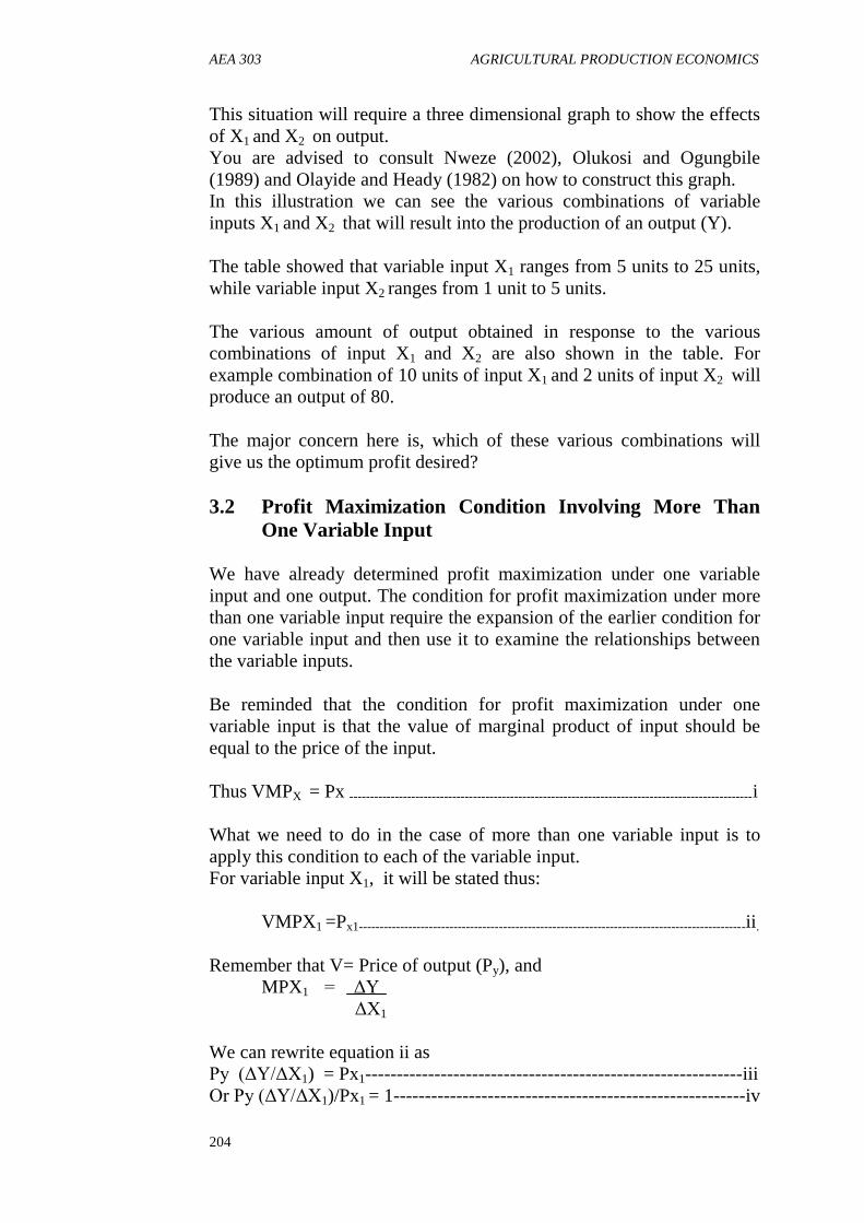
AEA 303 AGRICULTURAL PRODUCTION ECONOMICS
204
This situation will require a three dimensional graph to show the effects
of X1 and X2 on output.
You are advised to consult Nweze (2002), Olukosi and Ogungbile
(1989) and Olayide and Heady (1982) on how to construct this graph.
In this illustration we can see the various combinations of variable
inputs X1 and X2 that will result into the production of an output (Y).
The table showed that variable input X1 ranges from 5 units to 25 units,
while variable input X2 ranges from 1 unit to 5 units.
The various amount of output obtained in response to the various
combinations of input X1 and X2 are also shown in the table. For
example combination of 10 units of input X1 and 2 units of input X2 will
produce an output of 80.
The major concern here is, which of these various combinations will
give us the optimum profit desired?
3.2 Profit Maximization Condition Involving More Than
One Variable Input
We have already determined profit maximization under one variable
input and one output. The condition for profit maximization under more
than one variable input require the expansion of the earlier condition for
one variable input and then use it to examine the relationships between
the variable inputs.
Be reminded that the condition for profit maximization under one
variable input is that the value of marginal product of input should be
equal to the price of the input.
Thus VMPX = Px --------------------------------------------------------------------------------------------------i
What we need to do in the case of more than one variable input is to
apply this condition to each of the variable input.
For variable input X1, it will be stated thus:
VMPX1 =Px1----------------------------------------------------------------------------------------------ii.
Remember that V= Price of output (Py), and
MPX1 = ΔY
ΔX1
We can rewrite equation ii as
Py (ΔY/ΔX1) = Px1------------------------------------------------------------iii
Or Py (ΔY/ΔX1)/Px1 = 1--------------------------------------------------------iv

AEA 303 MODULE 5
205
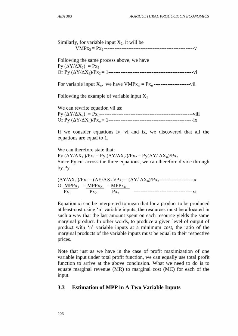
AEA 303 AGRICULTURAL PRODUCTION ECONOMICS
206
Similarly, for variable input X2, it will be
VMPx2 = Px2 ----------------------------------------------------v
Following the same process above, we have
Py (ΔY/ΔX2) = Px2
Or Py (ΔY/ΔX2)/Px2 = 1-------------------------------------------------vi
For variable input Xn, we have VMPxn = Pxn ---------------------vii
Following the example of variable input X1
We can rewrite equation vii as:
Py (ΔY/ΔXn) = Pxn------------------------------------------------------viii
Or Py (ΔY/ΔXn)/Pxn = 1-------------------------------------------------ix
If we consider equations iv, vi and ix, we discovered that all the
equations are equal to 1.
We can therefore state that:
Py (ΔY/ΔX1 )/Px1 = Py (ΔY/ΔX2 )/Px2 = Py(ΔY/ ΔXn)/Pxn
Since Py cut across the three equations, we can therefore divide through
by Py.
(ΔY/ΔX1 )/Px1 = (ΔY/ΔX2 )/Px2 = (ΔY/ ΔXn)/Pxn--------------------x
Or MPPx1 = MPPx2 = MPPxn
Px1 Px2 Pxn ----------------------------------xi
Equation xi can be interpreted to mean that for a product to be produced
at least-cost using „n‟ variable inputs, the resources must be allocated in
such a way that the last amount spent on each resource yields the same
marginal product. In other words, to produce a given level of output of
product with „n‟ variable inputs at a minimum cost, the ratio of the
marginal products of the variable inputs must be equal to their respective
prices.
Note that just as we have in the case of profit maximization of one
variable input under total profit function, we can equally use total profit
function to arrive at the above conclusion. What we need to do is to
equate marginal revenue (MR) to marginal cost (MC) for each of the
input.
3.3 Estimation of MPP in A Two Variable Inputs
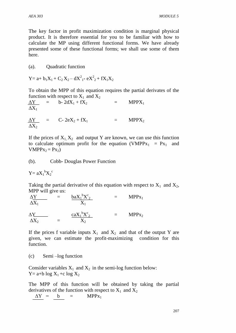
AEA 303 MODULE 5
207
The key factor in profit maximization condition is marginal physical
product. It is therefore essential for you to be familiar with how to
calculate the MP using different functional forms. We have already
presented some of these functional forms; we shall use some of them
here.
(a). Quadratic function
Y= a+ b1X1 + C2 X2 – dX2
1- eX22 + fX1X2
To obtain the MPP of this equation requires the partial derivates of the
function with respect to X1 and X2
ΔY = b- 2dX1 + fX2 = MPPX1
ΔX1
ΔY = C- 2eX2 + fX1 = MPPX2
ΔX2
If the prices of X1, X2 and output Y are known, we can use this function
to calculate optimum profit for the equation (VMPPx1 = Px1 and
VMPPx2 = Px2)
(b). Cobb- Douglas Power Function
Y= aX1bX2
c
Taking the partial derivative of this equation with respect to X1 and X2,
MPP will give us:
ΔY = baX1bX
c2 = MPPx1
ΔX1 X1
ΔY caX1
bX
c2 = MPPx2
ΔX2 = X2
If the prices f variable inputs X1 and X2 and that of the output Y are
given, we can estimate the profit-maximizing condition for this
function.
(c) Semi –log function
Consider variables X1 and X2 in the semi-log function below:
Y= a+b log X1 +c log X2
The MPP of this function will be obtained by taking the partial
derivatives of the function with respect to X1 and X2
ΔY = b = MPPx1

AEA 303 AGRICULTURAL PRODUCTION ECONOMICS
208
ΔX1 X1
ΔY = c = MPPx2
ΔX2 X2
For maximum profit and output, prices of X1 , X2 and Y are required.
(d). Square Root Function
Square root function involving two variable inputs can be written as
follows:
Y = a – bX1 – cX2 + dX1.5
+ eX2.5 + fX1
.5X2
.5
To calculate the MPP of this functional form, take the partial derivatives
of the function with respect to X1 and X2.
ΔY = – b+ .5dX1-.5
+ .5fX1-.5
X2.5
= MMPx1
ΔX1
ΔY = – c+ .5eX2-.5
+ .5fX1.5
X2-.5
= MMPx2
ΔX2
SELF-ASSESSMENT EXERCISE
Find the marginal physical product of this function Y = a ebx
1 + cX2
4.0 CONCLUSION
In this last unit of this module, we learnt about resource allocation
involving more than one variable input. We also looked at the condition
for profit maximization for more than one variable input and specifically
worked with profit maximization involving two variable inputs. We
finally used different functional forms to determine MPP of two variable
inputs. We can then conclude here that profit maximization involving
two or more variable inputs followed the same pattern with that of profit
maximization involving one variable input.
5.0 SUMMARY
The main points in this unit include the followings:
i. There are assumptions underlining the application of profit-
maximization condition for more than one variable input
ii. There are various outcomes of adjustments or variations between
inputs X1 and X2.
iii. Graphical expression of the relationship between two variable
inputs and one requires a three dimensional graph.
AEA 303 MODULE 5
209
iv. Profit maximizing condition for more than one variable input
follow the same step as in one variable input (VMPx = Px).
v. Profit maximization under more than one variable input requires
that
MPPx1 = MPPx2 = MPPxn
Px1 Px2 Pxn
vi. Marginal Physical Product (MPP) can be estimated using
different types of functional forms e.g. quadratic function, Cobb-
Douglas power function, semi-log function and square root
function.
6.0 TUTOR-MARKED ASSIGNMENT
Find the marginal physical product (MPP) of the following functional
forms:
(a) Y = a + b1X1 + b2X2 + b3X12 + b4X2
2
(b) Y = aX1b1
X2b2
(c) Y = a - b1X1 – b2X2 + b3X1.5 + b4X2
.5 + b5X1
.5X2
.5
7.0 REFERENCES/FURTHER READING
Abbot, J.C. and J.P. Makeham (1980). Agricultural Economics and
Marketing in the Tropics. London, Longman Publishers.
Adegeye, A.J. and J.S. Dittoh (1985). Essentials of Agricultural
Economics. Ibadan, Impact Publishers.
Nweze, N.J. (2002). Agricultural Production Economics: An
Introductory Text. Nsukka. AP Express Publishers.
Olayide, S.O. and Heady E.O. (1982). Introduction to Agricultural
Production Economics. Ibadan. University Press Ltd.
Olukosi, J.O. and A.O. Ogungbile (1989). Introduction to Agricultural
Production Economics: Principles and Applications. Zaria.
AGTAB Publishers Ltd.
Marshall A.C. (1998). Modern Farm Management Techniques. Owerri.
Alphabet Nigeria Publishers.
Reddy, S.S., P.R. Ram, T.V. Sastry and I.B. Devi (2004). Agricultural
Economics. New Delhi. Oxford and Ibh Publishers Ltd.

AEA 303 AGRICULTURAL PRODUCTION ECONOMICS
210
MODULE 4 FACTOR – FACTOR AND PRODUCT-
PRODUCT RELATIONSHIPS
Unit 1 Profit Maximization in Factor-Factor Relationships
Unit 2 Important Concepts in Factor-Factor Relationships
Unit 3 Product-Product Relationships
UNIT 1 PROFIT MAXIMIZATION IN FACTOR-
FACTOR RELATIONSHIPS
CONTENTS
1.0 Introduction
2.0 Objectives
3.0 Main Contents
3.1 Determination of Optimum Profit Using Production
Function Approach
3.2 Determination of Optimum Profit Using Total Profit
Function Approach
3.3 Constrained Profit Maximization
4.0 Conclusion
5.0 Summary
6.0 Tutor-Marked Assignment
7.0 References/Further Reading
1.0 INTRODUCTION
This is the first unit of module 4. The focus of the module is the
relationships between factor-factor and product-product. In this unit, we
shall focus our attention on profit maximization in factor-factor
relationships. Our major task in this unit will be determination of
optimum profit using either production function or total profit function
approach.
We shall also look at the effect of imposing constrain on optimum profit
2.0 OBJECTIVES
At the end of this unit, you should be able to:
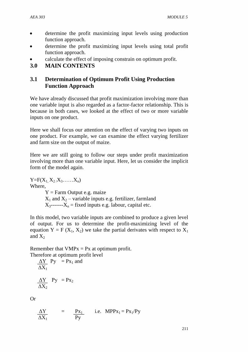
AEA 303 MODULE 5
211
determine the profit maximizing input levels using production
function approach.
determine the profit maximizing input levels using total profit
function approach.
calculate the effect of imposing constrain on optimum profit.
3.0 MAIN CONTENTS
3.1 Determination of Optimum Profit Using Production
Function Approach
We have already discussed that profit maximization involving more than
one variable input is also regarded as a factor-factor relationship. This is
because in both cases, we looked at the effect of two or more variable
inputs on one product.
Here we shall focus our attention on the effect of varying two inputs on
one product. For example, we can examine the effect varying fertilizer
and farm size on the output of maize.
Here we are still going to follow our steps under profit maximization
involving more than one variable input. Here, let us consider the implicit
form of the model again.
Y=F(X1, X2 /X3……Xn)
Where,
Y = Farm Output e.g. maize
X1 and X2 – variable inputs e.g. fertilizer, farmland
X3-------Xn = fixed inputs e.g. labour, capital etc.
In this model, two variable inputs are combined to produce a given level
of output. For us to determine the profit-maximizing level of the
equation Y = F (X1, X2) we take the partial derivates with respect to X1
and X2
Remember that VMPx = Px at optimum profit.
Therefore at optimum profit level
ΔY Py = Px1 and
ΔX1
ΔY Py = Px2
ΔX2
Or
ΔY = Px1 i.e. MPPx1 = Px1/Py
ΔX1 Py

AEA 303 AGRICULTURAL PRODUCTION ECONOMICS
212
ΔY = Px2 i.e. MPPx2 = Px2/Py
ΔX2 Py
We can separately solve for inputs X1 and X2 to arrive at profit
maximization if the two inputs does not interfere with each other. The
major concern here is that as output (Y) is held constant, we want to
look at the possibilities of substituting X1 for X2 or vice versa.
3.2 Determination of Optimum Profit Using Total Profit
Function Approach
Here we shall adopt similar approach when determining optimum profit
for one variable input using total profit function.
You will remember that under that approach we used the formula: ∏ =
TR – TC
Where,
∏ = Total Profit
TR = Total Revenue (RyY)
TC = Total Cost [(PxX) + F ]
We can expand this formular to cover two variable inputs as follows:
∏ = PyY – Px1 X1 – Px2 X2 – F -----------------------------------------------ii
To get the maximum we can differentiate this function with respect to
X1 and X2
Δ∏ = Py (∆Y/∆X1) – Px1 = 0 ---------------------------------------------iiii
∆X1
Δ∏ = Py (∆Y/∆X2) – Px2 = 0 ----------------------------------------------iv
∆X2
We can rewrite equation iii thus;
Py (ΔY/ΔX1) = Px1
ΔY/ΔX1 = Px1 / Py --------------------------------------------------------------v
Similarly, we can rewrite equation v thus:
Py (ΔY/ΔX2) = Px2
ΔY/ΔX2 = Px2 / Py -------------------------------------------------------------vi

AEA 303 MODULE 5
213
Thus arriving at the same conclusion when we used production function
approach.

AEA 303 AGRICULTURAL PRODUCTION ECONOMICS
214
SELF-ASSESSMENT EXERCISE
i. Use the profit function ∏ = PyY – Px1X1 – Px2X2 – F to proof
that VMPx1/Px1 = VMPx2/Px2 = 1
ii. Determine the minimum cost combination of inputs X1 and X2
for an output level of 250 units in the table below (Price of input
X1 N50 and that of X2 = N100):
Unit of X1 Unit of X2 Cost of X1 Cost of X2 Total outlay
1 30
2 25
3 20
4 15
5 10
6 5
3.3 Constrained Optimization
In all the output and profit maximization discussed so far, we have not
imposed any condition limiting the extent to which inputs can be
combined. Under that condition we are operating unconstrained output
or profit maximization.
What this then means is that farmers can achieve their objective function
without any constraint- no cash hindrance, no farmland limitation etc.
In reality, farmers may face some limitations in try to achieve their
objective function of profit maximization especially cash. Cash outlay
set a limit to which farmers can go in optimizing their profit function.
In other to impose limitation into the objective function of profit
maximization we need to subject the profit function to a constraint by
using Lagrange multiplier (ʎ). The product of this function can then be
added to the original profit function to form the new Lagrange function
Note the objective function:
∏ = PyY – (Px1 X2 + Px2X2 + F)-----------------------------------------------i
The budget constraint function or Lagrange multiplier
C = Px1X1 + Px2 X2 -------------------------------------------------------------ii
Set equation ii to zero
Px1 X1 + Px2 X2 – C = 0 -------------------------------------------------------iii
We can now add equations i and iii together
AEA 303 MODULE 5
215
∏ = PyY – Px1X1 – Px2X2 – F – (Px1X1 + Px2X2 - C)--------------------iv
Multiply through by Lagrange multiplier (ʎ) to obtain Lagrange function
as
∏ = PyY – Px1X1 – Px2X2 – F – ʎ(Px1X1 + Px2X2 - C)------V
We can now obtain our constrained optimum profit by taking the first-
order partial derative of the equation V with respect to X1, X2 and ʎ.
For detailed study of constrained profit maximization you can consult
Nweze (2002), Olayide and Heady (1982), Olukosi and Ogungbile
(1989), Marshall (1998) and other advanced books on Agricultural
production economics
4.0 CONCLUSION
In this unit, we discussed profit maximization in a factor-factor
relationship. In the unit, we showed how to determine optimum profit
using both production function and total profit function methods. We
went further to show how profit optimization can be achieved when
constraint is imposed on the objective function. We can conclude here
that, there is difference in unconstrained and constrained profit
maximization objective of farmers.
5.0 SUMMARY
The main points learnt in this unit include the followings:
1. Profit maximizing condition for factor-product involving more
than one variable input is the same with factor-factor
relationships
2. The same outcome were obtained when profit maximization in a
factor-factor relationship is determined using either production
function or total profit function approach.
3. Profit is maximized in a factor-factor relationship when MPPx1 =
Px1/Py and MPPx2 = Px2 / Py
4. Langrage function combines objective function with Lagrange
multiplier function in a constraint profit optimization.
6.0 TUTOR-MARKED ASSINGEMENT
1. Consider the production function of a yam farmer using fertilizer
(X1) and Yam Seed (X2) as variable inputs: Y = 20X1 + 4X2 –
2X1X2
Find
a. The optimum level of yam output (Y)
AEA 303 AGRICULTURAL PRODUCTION ECONOMICS
216
b. Levels of X1 and X2 required to produce this optimum
level of Y
7.0 REFERENCES/FURTHER READING
Abbot, J.C. and J.P. Makeham (1980). Agricultural Economics and
Marketing in the Tropics. London, Longman Publishers.
Adegeye, A.J. and J.S. Dittoh (1985). Essentials of Agricultural
Economics. Ibadan, Impact Publishers.
Ibitoye, S.J. and Idoko, D. (2009). Principles of Agricultural Economics.
Kaduna. Euneeks and Associates Publishers. Pp 82-92.
Nweze, N.J. (2002). Agricultural Production Economics: An
Introductory Text. Nsukka. AP Express Publishers.
Olayide, S.O. and Heady E.O. (1982). Introduction to Agricultural
Production Economics. Ibadan. University Press Ltd.
Olukosi, J.O. and A.O. Ogungbile (1989). Introduction to Agricultural
Production Economics: Principles and Applications. Zaria.
AGTAB Publishers Ltd.
Marshall A.C. (1998). Modern Farm Management Techniques. Owerri.
Alphabet Nigeria Publishers.
Reddy, S.S., P.R. Ram, T.V. Sastry and I.B. Devi (2004). Agricultural
Economics. New Delhi. Oxford and Ibh Publishers Ltd.

AEA 303 MODULE 5
217
UNIT 2 IMPORTANT CONCEPTS IN FACTOR –
FACTOR RELATIONSHIP
CONTENTS
1.0 Introduction
2.0 Objectives
3.0 Main Contents
3.1 Isoquant and Marginal Rate of Technical Substitution
(MRTS)
3.2 Elasticity of Input Substitution and Isocost Line
3.3 Determination of Least Cost Combination
3.4 Isocline, Ridge line and Input Expansion Path
4.0 Conclusion
5.0 Summary
6.0 Tutor-Marked Assignment
7.0 Reference Further Reading
1.0 INTRODUCTION
In unit 1 of this module, we discussed profit maximization in factor-
factor relationship. We illustrated this using two different approaches.
The first method involved the use of production function approach to
determine optimum profit. The second method involved the use of total
profit function approach. We equally determined profit maximization
conditions when constrain is imposed.
In this unit 2 of the module, we shall go a step further to consider some
important concepts related to factor-factor relationships. Notable among
these concepts are: isoquant, marginal rate of technical substitution
(MRTS), Elasticity of input substitution, isocost and determination of
least cost combinations. Other concepts are: Isocline, Ridgeline and
Expansion path.
2.0 OBJECTIVES
At the end of the unit, you should be able to:
define Isoquant
explain the relationship between Isoquant and MRTS
calculate the elasticity of input substitution
plot the graphs and explain the meanings of Isocline, ridge line
and expansion path.
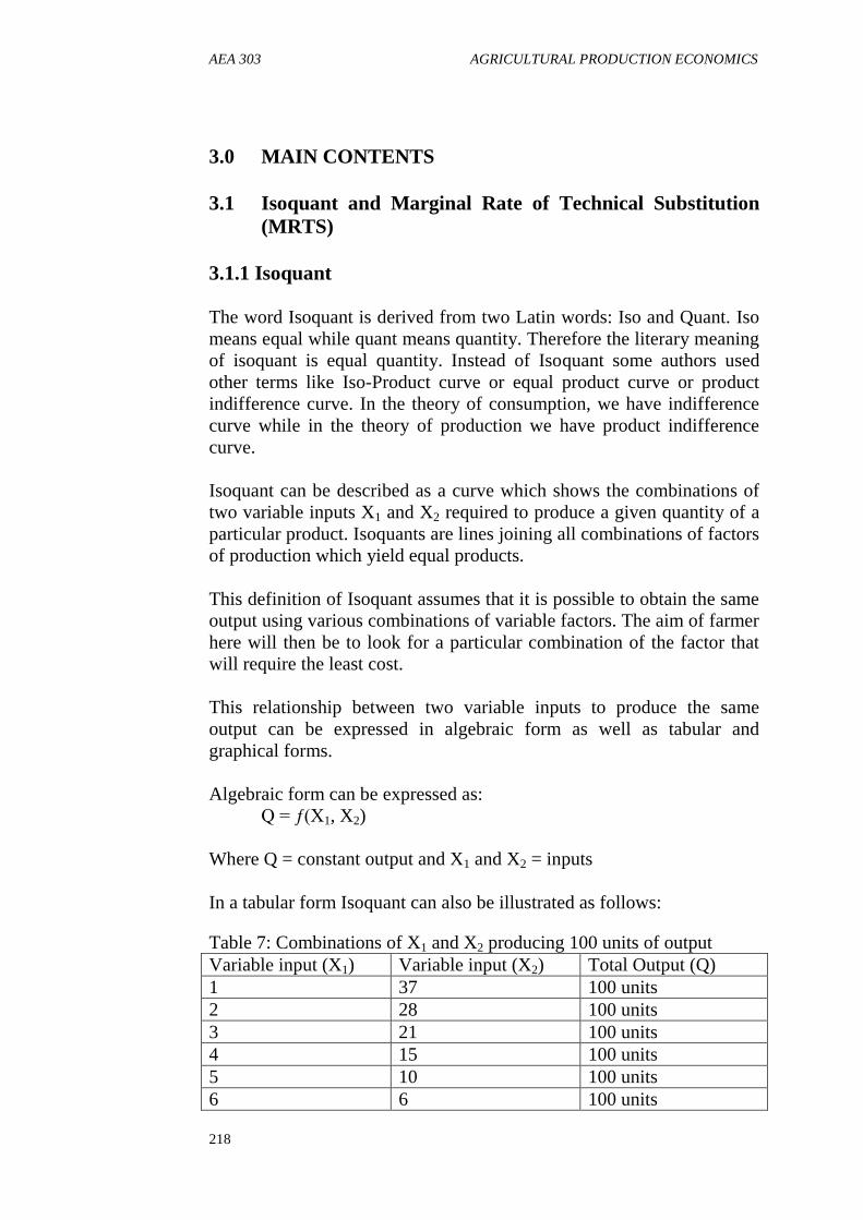
AEA 303 AGRICULTURAL PRODUCTION ECONOMICS
218
3.0 MAIN CONTENTS
3.1 Isoquant and Marginal Rate of Technical Substitution
(MRTS)
3.1.1 Isoquant
The word Isoquant is derived from two Latin words: Iso and Quant. Iso
means equal while quant means quantity. Therefore the literary meaning
of isoquant is equal quantity. Instead of Isoquant some authors used
other terms like Iso-Product curve or equal product curve or product
indifference curve. In the theory of consumption, we have indifference
curve while in the theory of production we have product indifference
curve.
Isoquant can be described as a curve which shows the combinations of
two variable inputs X1 and X2 required to produce a given quantity of a
particular product. Isoquants are lines joining all combinations of factors
of production which yield equal products.
This definition of Isoquant assumes that it is possible to obtain the same
output using various combinations of variable factors. The aim of farmer
here will then be to look for a particular combination of the factor that
will require the least cost.
This relationship between two variable inputs to produce the same
output can be expressed in algebraic form as well as tabular and
graphical forms.
Algebraic form can be expressed as:
Q = ƒ(X1, X2)
Where Q = constant output and X1 and X2 = inputs
In a tabular form Isoquant can also be illustrated as follows:
Table 7: Combinations of X1 and X2 producing 100 units of output
Variable input (X1) Variable input (X2) Total Output (Q)
1 37 100 units
2 28 100 units
3 21 100 units
4 15 100 units
5 10 100 units
6 6 100 units
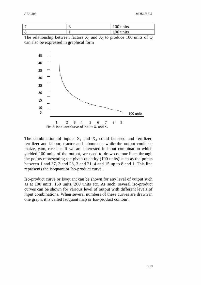
AEA 303 MODULE 5
219
7 3 100 units
8 1 100 units
The relationship between factors X1 and X2 to produce 100 units of Q
can also be expressed in graphical form
The combination of inputs X1 and X2 could be seed and fertilizer,
fertilizer and labour, tractor and labour etc. while the output could be
maize, yam, rice etc. If we are interested in input combination which
yielded 100 units of the output, we need to draw contour lines through
the points representing the given quantity (100 units) such as the points
between 1 and 37, 2 and 28, 3 and 21, 4 and 15 up to 8 and 1. This line
represents the isoquant or Iso-product curve.
Iso-product curve or Isoquant can be shown for any level of output such
as at 100 units, 150 units, 200 units etc. As such, several Iso-product
curves can be shown for various level of output with different levels of
input combinations. When several numbers of these curves are drawn in
one graph, it is called Isoquant map or Iso-product contour.
100 units
1 2 3 4 5 6 7 8 9 Fig. 8: Isoquant Curve of inputs X1 and X2
45
5
10
15
20
25
30
35
40

AEA 303 AGRICULTURAL PRODUCTION ECONOMICS
220
In Isoquant map Q3 > Q2 > Q1, therefore Q3 can be 200 units, while Q2
could be 150 units and Q1 can be 100 units.
Characteristic Features of Isoquant
(a) Isoquants slope downwards from left to right; this means that
Isoquant have negative slope. In order words, if we reduce the
quantity of input X1, we must increase the quantity of input X2 in
order to maintain the same level of output.
(b) Isoquants are convex to the origin: The amount by which we have
to increase input X1 divided by the amount by which we have to
reduce input X2 is referred to as the rate of technical substitution.
The absolute slope of Isoquant decrease as we move from left to
the right of the curve indicating diminishing rate of technical
substitution. As a result of diminishing marginal rate of technical
substitution each one unit of input added replaces less and less
than the previous unit.
(c) The Curves are Smooth and Continuous
This means that both inputs are infinitely divisible. Therefore we
can easily take any fractional value of them. In other words, we
are not forced to use input X1 and X2 in a fixed proportion.
(d) Output Levels Increase as we Move away from the Origin
Isoquant representing higher level of output are placed further
away from the origin and vice versa.
Q3
Q2
Q1
Input X1
Input X2
Fig. 9: Iso-product contour or Isoquant Map
AEA 303 MODULE 5
221
(e) Isoquants are non-intersecting
Two Isoquants cannot intersect each other because the same
combination of two inputs cannot produce two different levels of
output.
3.1.2 Marginal Rate of Technical Substitution (MRTS)
The slope of Isoquant measured the marginal rate of technical
substitution. It is the rate of exchange between two productive resources
which are equally preferred. In order words, it is the rate at which inputs
substitute for each other to maintain a constraint output. MRTS indicates
the absolute amount by which one input is decreased or given up in
order to gain a unit of another input by one unit in the process of
substitution.
Marginal Rate of Technical Substitution (MRTS) also called Marginal
Rate of Input Substitution (MRIS) can be computed using the following
equation.
MRTS = Quantity of input sacrificed = ∆X2
Quantity of input gained ∆X1
Where
X1 = Added input, and
X2 = Replaced input
This showed the amount by which X2 must be decreased to maintain the
same level of output when X1 is increased by one unit. The characteristic
features of MRTS include the followings:
i. MRTS is the slope of Isoquant
ii. Isoquant slope downward from left to the right and therefore
MRTS is negative
iii. MRTS is equal to the ratio of the marginal products of the inputs
i.e ∆X1 = MPPx2
∆X2 MPPx1
This relationship can lead to three different forms of input substitution:
a. Constant rate of input substitution
b. Diminishing Rate of input substitution, and
c. Increasing Rate of Input substitution
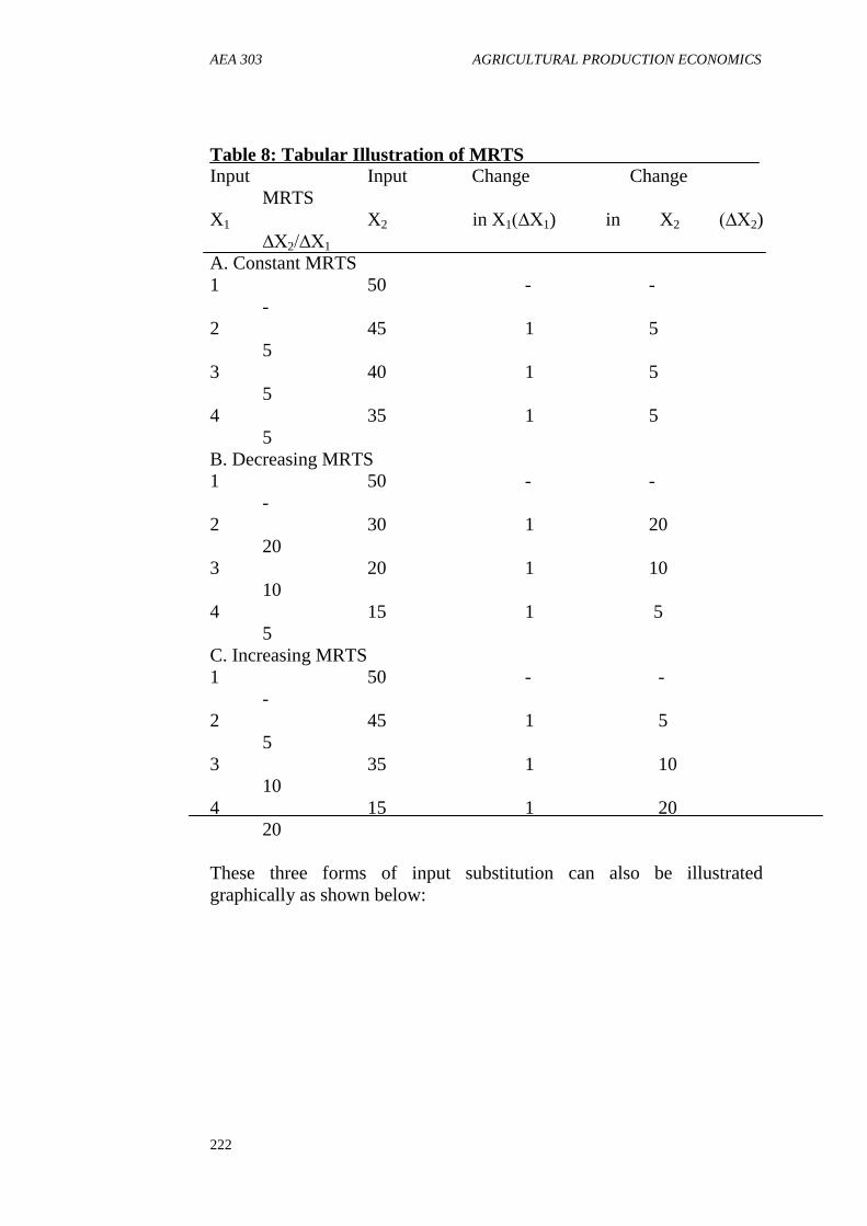
AEA 303 AGRICULTURAL PRODUCTION ECONOMICS
222
Table 8: Tabular Illustration of MRTS
Input Input Change Change
MRTS
X1 X2 in X1(∆X1) in X2 (∆X2)
∆X2/∆X1
A. Constant MRTS
1 50 - -
-
2 45 1 5
5
3 40 1 5
5
4 35 1 5
5
B. Decreasing MRTS
1 50 - -
-
2 30 1 20
20
3 20 1 10
10
4 15 1 5
5
C. Increasing MRTS
1 50 - -
-
2 45 1 5
5
3 35 1 10
10
4 15 1 20
20
These three forms of input substitution can also be illustrated
graphically as shown below:
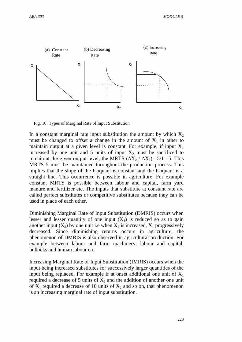
AEA 303 MODULE 5
223
In a constant marginal rate input substitution the amount by which X2
must be changed to offset a change in the amount of X1 in other to
maintain output at a given level is constant. For example, if input X1
increased by one unit and 5 units of input X2 must be sacrificed to
remain at the given output level, the MRTS (∆X2 / ∆X1) =5/1 =5. This
MRTS 5 must be maintained throughout the production process. This
implies that the slope of the Isoquant is constant and the Isoquant is a
straight line. This occurrence is possible in agriculture. For example
constant MRTS is possible between labour and capital, farm yard
manure and fertilizer etc. The inputs that substitute at constant rate are
called perfect substitutes or competitive substitutes because they can be
used in place of each other.
Diminishing Marginal Rate of Input Substitution (DMRIS) occurs when
lesser and lesser quantity of one input (X1) is reduced so as to gain
another input (X2) by one unit i.e when X2 is increased, X1 progressively
decreased. Since diminishing returns occurs in agriculture, the
phenomenon of DMRIS is also observed in agricultural production. For
example between labour and farm machinery, labour and capital,
bullocks and human labour etc.
Increasing Marginal Rate of Input Substitution (IMRIS) occurs when the
input being increased substitutes for successively larger quantities of the
input being replaced. For example if at onset additional one unit of X1
required a decrease of 5 units of X2 and the addition of another one unit
of X1 required a decrease of 10 units of X2 and so on, that phenomenon
is an increasing marginal rate of input substitution.
X2
X2
(c) Increasing
Rate
Fig. 10: Types of Marginal Rate of Input Substitution
X2
X1 X1
X2
(b) Decreasing
Rate
(a) Constant
Rate

AEA 303 AGRICULTURAL PRODUCTION ECONOMICS
224

AEA 303 MODULE 5
225
3.2 Elasticity of Input Substitution and Isocost Line
3.2.1 Elasticity of Input Substitution
We have already discussed elasticity of production under factor-product
relationship Elasticity of input substitution under factor-factor
relationship is similar to that of elasticity of production. Instead of
looking at input X and output Y, we will now focus on input X1 and
input X2.
Therefore elasticity of input substitution (Es) can be defined as:
Es = Percentage Change in Input X1
Percentage Change is Input X2
i.e ∆X1 ÷ ∆X2 = ∆X1 × X2
X1 X22 ∆X2 X1
Or
MRSx2 for X1 . X2 / X1
In a technical input substitution the slope of Isoquant is negative and
therefore the elasticity of input substitution under that condition is also
negative. This is because as one input is increasing the other one is
decreasing and vice versa.
3.2.2 Isocost Line
Isocost line is also known as Budget line or price line or Iso-outlay line.
It is the locus of all combination of two inputs that can be purchased
with a given outlay of funds.
For Isocost line to be drawn we must determine the total outlay and the
prices per unit of X1 and X2.
Let us consider two variable inputs X1 and X2 if a farmer has a fund of
N200 to spend on the two inputs and the price per unit of X1 is N10
while the price per unit of X2 is N5. If the farmer spend the whole fund
on input X1, he can purchased 20 units (N200 / N10 = 20) and if the
farmer spend the whole of the fund on input X2 alone he can purchase
40 units (N200 / N5 = 40). In between these two points we can plot the
Isocost line showing the various combinations of X1 and X2 at a total
outlay of N200
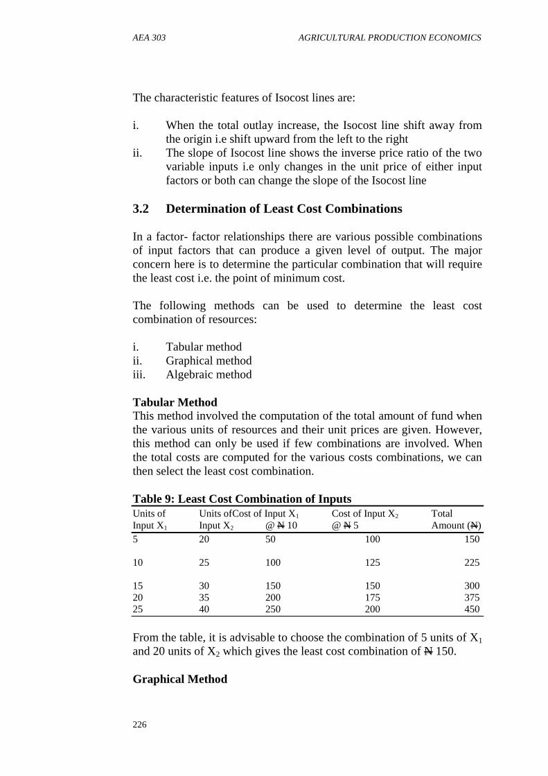
AEA 303 AGRICULTURAL PRODUCTION ECONOMICS
226
The characteristic features of Isocost lines are:
i. When the total outlay increase, the Isocost line shift away from
the origin i.e shift upward from the left to the right
ii. The slope of Isocost line shows the inverse price ratio of the two
variable inputs i.e only changes in the unit price of either input
factors or both can change the slope of the Isocost line
3.2 Determination of Least Cost Combinations
In a factor- factor relationships there are various possible combinations
of input factors that can produce a given level of output. The major
concern here is to determine the particular combination that will require
the least cost i.e. the point of minimum cost.
The following methods can be used to determine the least cost
combination of resources:
i. Tabular method
ii. Graphical method
iii. Algebraic method
Tabular Method
This method involved the computation of the total amount of fund when
the various units of resources and their unit prices are given. However,
this method can only be used if few combinations are involved. When
the total costs are computed for the various costs combinations, we can
then select the least cost combination.
Table 9: Least Cost Combination of Inputs
Units of Units of Cost of Input X1 Cost of Input X2 Total
Input X1 Input X2 @ N 10 @ N 5 Amount (N)
5 20 50 100 150
10 25 100 125 225
15 30 150 150 300
20 35 200 175 375
25 40 250 200 450
From the table, it is advisable to choose the combination of 5 units of X1
and 20 units of X2 which gives the least cost combination of N 150.
Graphical Method
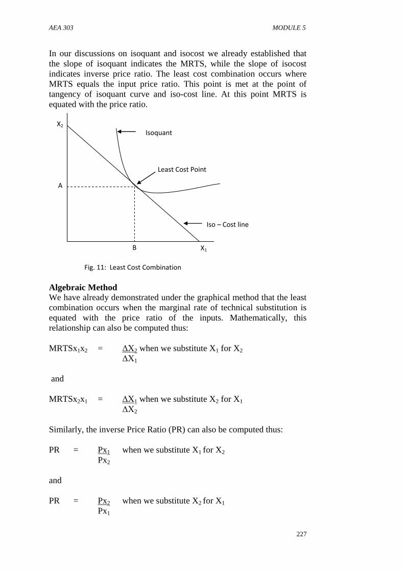
AEA 303 MODULE 5
227
In our discussions on isoquant and isocost we already established that
the slope of isoquant indicates the MRTS, while the slope of isocost
indicates inverse price ratio. The least cost combination occurs where
MRTS equals the input price ratio. This point is met at the point of
tangency of isoquant curve and iso-cost line. At this point MRTS is
equated with the price ratio.
Algebraic Method
We have already demonstrated under the graphical method that the least
combination occurs when the marginal rate of technical substitution is
equated with the price ratio of the inputs. Mathematically, this
relationship can also be computed thus:
MRTSx1x2 = ΔX2 when we substitute X1 for X2
ΔX1
and
MRTSx2x1 = ΔX1 when we substitute X2 for X1
ΔX2
Similarly, the inverse Price Ratio (PR) can also be computed thus:
PR = Px1 when we substitute X1 for X2
Px2
and
PR = Px2 when we substitute X2 for X1
Px1
X2
A
B
Iso – Cost line
Isoquant
X1
Fig. 11: Least Cost Combination
Least Cost Point

AEA 303 AGRICULTURAL PRODUCTION ECONOMICS
228
Algebraically, least-cost input combination is obtained when the
producer employs inputs in such a way as to equate the marginal rate of
technical substitution to the ratio of their prices.
3.4 Isocline, Ridgeline and Expansion Path
3.4.1 Isocline
Isocline is defined as a line which connects points of equal slope on a
production surface. This definition implies that isoclines pass through
points of equal MRTS on an isoquant map. This also means that it is
possible to have more than one isocline on a production surface as there
are different MRTS on an isoquant. However, the isoclines for each
MRS is constant.
3.4.2 Input Expansion Path
Expansion path can be described as an isocline that connects the points
of least cost combination for different values of output. Expansion path
is a line or curve on which the slope of isoquant (MRTS) equals the
slope of iso-cost line (price ratio). The expansion path indicates the best
way of producing different levels of output given the prices of inputs.
Since expansion path correspond to the point where MRTS equate price
ratio, we can use this relationship to determine the point of maximum
profit and the corresponding levels of output and input factors that will
maximize profit on an expansion path.
That is, where VMPx1 = Px1 and VMPx2 = Px2.
Expansion path
Isoquant
Iso-cost
X2
X1 0
Fig. 12: Expansion Path

AEA 303 MODULE 5
229
3.4.3 Ridgeline
Ridgeline is a line which connects points of zero slope on the successive
isoquants. Ridgeline shows the boundaries for the stages of production
function in the factor-factor relationship where the MPP and MRTS for
each input = 0. It marks the limit of the efficiency of resource use. Ridge
line represents the point of maximum output for each input given a fixed
quantity of other inputs. Ridge line represents the limit of input
substitution. Beyond the line, it is not possible to substitute inputs.
Beyond the lower ridgeline and above the upper ridgeline MPP is
negative.
SELF-ASSESSMENT EXERCISE
i. Define the following terms: Isoquant; Isocost line; Expansion
path; and Marginal Rate of Technical Substitution.
ii. Determine the minimum cost combination of inputs X1 and X2
for an output level of 200 units given the following table:
Units of X1 Units of X2 Cost of X1 Cost of X2 Total Amount
4 24
6 18
8 16
10 15
12 17
14 14
16 10
18 12
X1
X2
0
Fig. 13: Ridge lines
Isoquant
Ridgeline for X1
Ridgeline for X2

AEA 303 AGRICULTURAL PRODUCTION ECONOMICS
230
20 14
Px1 = N50 and Px2 = N100
4.0 CONCLUSION
We discussed in this unit some important concepts in factor-factor
relationship. The unit shed light on the meaning of concepts like
isoquant, marginal rate of technical substitution, elasticity of input
substitution, iso-cost, iso-cline, ridgeline and expansion path. This unit
also discussed the determination of least cost combination of input
factors.
5.0 SUMMARY
The main points learnt in this unit include the followings:
i. Isoquant is a curve which shows the combination of two inputs
required to produce a given quantity of a particular product
ii. Isoquant slope downward
iii. Isoquant are convex to the origin
iv. Isoquant curves are smooth and continuous
v. Isoquant are non intersecting
vi. MRTS is the slope of isoquant
vii. ΔX1/ΔX2 = MPPx2/MPPx1
viii. Marginal Rate of Input Substitution can be constant, decreasing
or increasing
ix. Elasticity of Input Substitution is computed as ΔX1/ΔX2 . X2/ or
MRSx2 for X1 . X2/X1
x. Iso-cost line is also known as budget line or price line or iso-
outlay line
xi. Least cost combination can be determined using tabular method,
graphic method and algebraic method.
xii. \Isocline passes through points of equal MRTS on an isoquant
map
xiii. Expansion path is also an isocline that passes through the points
of least cost combination for different levels of output
xiv. Ridgeline shows the limit of maximum output for each input
given a fixed quantity of other inputs.
6.0 TUTOR-MARKED ASSIGNMENT
1. Explain the meaning of the following concepts:
i. Isoquant
ii. Marginal Rate of Technical Substitution
iii. Elasticity of Input Substitution
iv. Isocost line
AEA 303 MODULE 5
231
v. Expansion Path
7.0 REFERENCES/FURTHER READING
Abbot, J.C. and J.P. Makeham (1980). Agricultural Economics and
Marketing in the Tropics. London, Longman Publishers.
Adegeye, A.J. and J.S. Dittoh (1985). Essentials of Agricultural
Economics. Ibadan, Impact Publishers.
Doll, J.P. and Orazen, P. (1978). Production Economics: Theory with
Application. USA, John Willey and Sons Publishers.
Ibitoye, S.J. and Idoko, D. (2009). Principles of Agricultural Economics.
Kaduna. Euneeks and Associates Publishers. Pp 82-92.
Nweze, N.J. (2002). Agricultural Production Economics: An
Introductory Text. Nsukka. AP Express Publishers.
Olayide, S.O. and Heady E.O. (1982). Introduction to Agricultural
Production Economics. Ibadan. University Press Ltd.
Olukosi, J.O. and A.O. Ogungbile (1989). Introduction to Agricultural
Production Economics: Principles and Applications. Zaria.
AGTAB Publishers Ltd.
Marshall A.C. (1998). Modern Farm Management Techniques. Owerri.
Alphabet Nigeria Publishers.
Reddy, S.S., P.R. Ram, T.V. Sastry and I.B. Devi (2004). Agricultural
Economics. New Delhi. Oxford and Ibh Publishers Ltd.
AEA 303 AGRICULTURAL PRODUCTION ECONOMICS
232
UNIT 3 PRODUCT- PRODUCT RELATIONSHIPS
CONTENTS
1.0 Introduction
2.0 Objectives
3.0 Main Contents
3.1 Types of product- product relationships
3.2 Production possibility curve (PPC)
3.3 Iso-Revenue and Output Expansion Path
3.4 Determination of Optimum Revenue Combination
3.5 Profit maximization under product-product relationship
4.0 Conclusion
5.0 Summary
6.0 Tutor-Marked Assignment
7.0 References/Further Reading
1.0 INTRODUCTION
In unit 2 of this module, we discussed some important concepts in
factor-factor relationship. Among the concepts we explain the meaning
of Isoquant and Marginal Rate of Technical Substitution we also explain
the meaning of Iso-cost line and elasticity of input substitution. In that
unit, we determined the least cost combination using tabular method,
graphic method and algebraic method. Finally, we also looked at the
relationship between the concepts of Isocline, expansion path and
ridgeline. In this unit 3 of this module we shall identify the various types
of product – product relationship, plot the graph of production
possibility curve and explain the concepts of Iso-revenue and output
expansion path. In the concluding part of this unit we will explain how
to determine the optimum revenue combination.
2.0 OBJECTIVES
At the end of this unit, you should be able to:
identify and explain the meaning of the four types of product-
product relationships
explain the concept of production possibility curve
describe the concepts of Iso-revenue and output expansion path
determine the optimum revenue combination
explain the concept of production possibility curve involving
more than one variable input.
AEA 303 MODULE 5
233
3.0 MAIN CONTENTS
3.1 Types of Product-Product Relationships
Product-product relationship is a production relationship involving two
different enterprises with a fixed amount of input factor. It involves the
consideration of a fixed amount of input factor and the various
combinations of two products that can be obtained from it. It involves
the determination of the optimum combination of two enterprises y1 and
y2 that can be produced given the fixed amount of resource x. In other
words, to produce more hectares of crop Y1 with a fixed hectares of
land will imply the production of less hectares of crop Y2 and vice
versa.
The implicit production function of a product- product relationship can
be written as:
X = ƒ (Y1, Y2)
Where
X = Fixed input (e.g. Land)
Y1 = Enterprise 1 (e.g. Maize)
Y2 = Enterprise 2 (e.g. Cowpea)
Agricultural products bear several relationships with one another on the
farm some of these relationships that exist among farm enterprises
include the followings:
a. Competitive Products
b. Joint Products
c. Complementary Products, and
d. Supplementary Products
3.1.1 Competitive Products
Competitive products are among the types of relationships that exist in
product-product relationships. Two products are said to be competitive
when increase in the level of production of one results in decrease in the
level of production of another and vice versa, given the fixed amount of
resources.
The marginal rate of product substitution in competitive product is
negative. This means that increasing the output of one product will lead
to decreasing the output of the other product. Competitive products
require the same set of inputs and one product can only be increased by

AEA 303 AGRICULTURAL PRODUCTION ECONOMICS
234
diverting resources the quantity of resources and output of the other
product. Example of competitive products in agriculture include: maize
and sorghum, Cassava and Yam, Cocoa and Rubber, Sheep and Goat
etc.
3.1.2 Joint Products
Joint products are two products which must be produce together by a
given production process. In joint products, the two products are
combined in fixed proportions and it is impossible to produce one
without the other. However, on the long run, technology can make the
manipulation of the proportions of the two products possible. Almost all
agricultural products are produce in conjunction with other products.
Examples of joint products in agricultural production are: Mutton and
wool, cotton lint and cotton seed, palm oil and palm kernels, beef and
hides etc. the production possibility curve for joint products is
represented by a point which could be as many as the levels of
resources.
3.1.3 Complementary Products
Complementary products occur when an increase in the output of one
product results in an increase in the output of the other product with
productive resources held constant in amount. In other words, a shift of
resources form product Y1 to product Y2 will increase the two products.
The marginal rate of product substitution in complementary products is
greater than zero (positive). This means that increasing the production of
output Y1 by diverting the use of more resources to its production will
lead to increase in the production of product Y2
The two products do not compete for the resources. One of the products
contributes an element of production required by another thereby
helping each other in production. This occurrence is a common
phenomena in agricultural production. Examples of such occurrence in
agriculture include the followings: legume crop and Maize crop, the
legume fixes nitrogen thereby improving the soil fertility for the maize
production. Livestock and sorghum, sorghum provides straws for the
livestock to feed and livestock in turn provides farm yard manure for the
sorghum.
3.1.4 Supplementary Products
Two products are said to be supplementary if the quantify of one
product can be increase without increasing or decreasing the quantity of
the other product. The supplementary products occurs when enterprises
AEA 303 MODULE 5
235
can be produced only during a distinct and limited period of the year and
the resources employed in the production give off a flow of services
throughout the period.
Examples of supplementary products in agriculture include the
followings:
i. The use of family labour for the production of broilers and
tomatoes
ii. The use of tractor for ploughing cassava plot at the beginning of
rainy season and later use for ploughing in dry season vegetable
gardening
In general since crop production is seasonal most resources are slack
during the off season, farmers can then make the best use of this off
season period to introduce supplementary enterprise that will make use
of these slack resources.
3.2 Production Possibility Curve (PPC)
Production Possibility Curve (PPC) is a curve which shows how one
output Y1 can be transformed into another output Y2 by reducing output
Y1 and transferring the resources thus saved into production of Y2. It is
based on the assumption that resources on the economy are fixed in total
and therefore the alternative combinations of Y1 and Y2 are technically
feasible PPC represents all possible combinations of two products Y1
and Y2 that could be produced with given amount of resources. The
main purpose of PPC is to determine the most profitable combination of
enterprise given the resource limitation facing the farmer.
The characteristic features of PPC include the followings:
a. PPC is concave to the origin
b. A change in the level of input resource will shift the curve
c. The slope of PPC indicates the Marginal Rate of Product
Substitution (MRPS).
PPC is also called Iso-revenue curve or Iso-factor curve because each
point to the curve represents combinations of outputs from equal
amounts of input. PPC is also known as opportunity curve because the
curve presents to the farmer all the production opportunities between
products Y1 and Y2 with a given amount of resources
The slope of the PPC indicates the rate at which one product is
transformed into another product and therefore called transformation

AEA 303 AGRICULTURAL PRODUCTION ECONOMICS
236
curve. In conclusion, PPC is also known as Iso-resource curve or
transformation curve.
PPC can be illustrated in a tabular form as follows:
Table 10: Production Possibility Schedule for Products Y1 and Y2
Input X Output Y1 Output Y2 MPP of Y1
MPP of Y2
(Farm Size) (Maize) (Cowpea)
0 0 0 -
-
1 13 16 13
16
2 20 26 7
10
3 26 34 6
8
4 31 40 5
6
5 35 44 4
4
The table shows that the farmer has a limited input of 5 hectares of farm
land and has two alternatives of using the land for the production of
maize (Y1) and cowpea (Y2). The alternatives are using the entire 5
hectares of land for the production of Maize (Y1) alone or using it to
produce cowpea (Y2) alone. In between these two extremes, there are
other available options like using 1 hectare for one crop and the
remaining 4 hectares for the other, 2 hectares for one and 3 hectares for
the other. These opportunities can be present in another table
Table 11: Production Possibilities for 5 hectares of land
Input X Output Y1 Input X Output Y2
Hectares of Land (Maize) Hectares (Cowpea)
0 0 5 44
1 13 4 40
2 20 3 34
3 26 2 26
4 31 1 16
5 35 0 0

AEA 303 MODULE 5
237
The different levels of farm land (X) and the corresponding levels of
maize output (Y1) and cowpea output (Y2) represent two production
functions.
PPC is a convenient method of showing the two production functions in
a single graph.
Fig. 14: Production Possibility Curve with 5 Hectares of Farm Land
The PPC as plotted on the graph is used to compare two production
functions on the same graph subject to the limit of the available input.
Let us consider the table and the graph above; if the farmer has only 5
hectares of farmland to produce Maize (Y1) cowpea (Y2), by using all
the 5 hectares of land for the production of Maize (Y1), he will produce
35 units of Maize and 0 unit of cowpea. Alternatively, by using all the 5
hectares of land for the production of cowpea, he will produce 44 units
of cowpea and 0 unit of maize. There are then other possibilities apart
from these two extremes. For example if 3 hectares of land is used for
maize production he will obtain 26 units and the remaining 2 hectares
available for cowpea will also yield 26 units of cowpea. One hectare
applied to maize and four hectares to cowpea will results in 13 units of
maize and 40 units of cowpea.
Y2
Y1
10 20 30 40 50
30
20
10
0

AEA 303 AGRICULTURAL PRODUCTION ECONOMICS
238
3.3 Iso-Revenue Line and Output Expansion Path
3.3.1 Iso-Revenue Line
Iso-revenue line is a line which defines all possible combinations of two
products which would yield equal revenue. In other words, it is the locus
of pints of various combinations of Y1 and Y2 whose sales yield the same
revenue.
Let us assumed that the total revenue for two products
Y1 and Y2 to be:
TR = P1 Y1 + P2 Y2
Where P1 = price per unit of product Y1
P2 = Price per unit of product Y2
Let us assumed also that the total revenue from the two products Y1 and
Y2 = N200 and the unit price of product Y1 is N2.00 and unit price of
product is N5.00 . Which means that 100 units of Y1 could be obtained
if only Y1, is produced (ie. N200/N2=100). Alternatively if only Y2 is
produced we can also obtain 40units (N200/ N5=40). In between
100units of Y1 and 40units of Y2, several other combinations could also
earn N200. For example 50units of Y1 and 20units of Y2 will also earn
N200. We can then join all these various points together to form Iso-
revenue line.
10 20 30 40
105
90
75
60
45
30
15
Y1 (100, 0)
(40, 0)
Y2

AEA 303 MODULE 5
239
Fig. 15: 1so-revenue line for total revenue of N200
The ratio of the unit price of the two products determines the slope of
the ISO-revenue line. The characteristic features of the ISO-revenue line
include the followings;
a. ISO-revenue lines are parallel to each other
b. The slope of the ISO-revenue line indicates the inverse price ratio
of the products
c. ISO-revenue line is a straight line
d. ISO-revenue line shifts upward away from the origin as total
revenue increases
SELF-ASSESSMENT EXERCISE
Apart from the combinations of 100 and 0, 0 and 40 and 50 and 20 units
obtained for total revenue of N200 with price of Y1=N2 and price of
Y2=N5, find 5 other possible combinations between Y1 and Y2.
3.3.2 Output Expansion Path
Output expansion path is the line which connects the points of optimal
product combinations on the successive production possibility curves. It
is possible to have different levels of total revenue target and each level
produce different ISO-revenue lines. Similarly, different total
combinations of two products will also produce different production
possibility curves. It is then possible to present the production
possibility curves for these different units with their respective ISO-
revenue lines of equal gradient on the same graph. The line connecting
the maximum revenue points is the output expansion path.
Y1
Y2
Output Expansion Path
Production Possibility curve
Iso-revenue line

AEA 303 AGRICULTURAL PRODUCTION ECONOMICS
240
Fig. 16: PPC and Iso-revenue for different units of Y1 and Y2
3.4 Determination of Optimum Resource Combination
In other to obtain the point of optimum resource combination we need to
know the combinations of the two products that will results into this
optimum net revenue. The following methods can be used to determine
the optimum product combinations to maximize net revenue:
a. Tabular method
b. Marginal Rate of Product Substitution (Algebraic Method)
c. Graphical Method
3.4.1 Tabular Method
In other to determine the maximum revenue combination from
production possibility data, we need to know the unit price for each
product to compute the total revenue of each output combination. The
output combination which yields the maximum revenue will be chosen
as the maximum revenue combination.
Let us consider our production possibility data where the price of maize
(Y1)=N2.0 and the price of cowpea (Y2)=N5.0
Table 12: Tabular Computation of Optimum Output Combination
Maize Cowpea Revenue from Revenue from Total
(Y1) (Y2) maize (P1Y2) Cowpea (P2Y2) Revenue
(P1Y2 + P2Y2)
0 44 0 220 220
13 40 26 200 226
20 34 40 170 210
26 26 52 130 182
31 16 62 80 142
35 0 70 0 70
From the table, the combination of 13units of maize (Y1) output and 40
units of cowpea (Y2) output gives the maximum income of N226
3.4.2 Marginal Rate of Product Substitution (Algebraic
Method)

AEA 303 MODULE 5
241
Marginal Rate of Product substitution (MRPS) is the absolute amount by
which one product is decreased in other to gain another product by one
unit. In case of two products y1 and y2, MRPS of y1 for y2 implies that
the amount of Y2 to be given up in order to gain y1 by one unit while
input use remain constant.
Mathematically written as
MRPS=No of units of replaced product = ΔY2
No of units of replacing product ΔY1
In this case, Y2 is the replaced product and y1 is the replacing product.
Just as we have in the case of factor-factor, product-product can also
substitute at constant rate, decreasing rate and increasing rate. We have
already established earlier that optimum revenue combination obtained
where MRPS is equated to the price ratio of the two products.
Therefore, the price ratio (PR) can be computed as
PR=Price per unit of replacing product =Py1
Price per unit of replaced product Py2
Therefore optimum combination of product is obtained as follows:
Y2 = Py1 OR Y1 = Py2
Y1 Py2 Y2 Py1
3.4.3 Graphical Method
In order to determine the optimum revenue combination of two products
using graphical approach, we need production possibility data and the
Iso-revenue data. Just as we demonstrated under the output expansion
path, both PPC and Iso-revenue can be plotted on the same graph.
We have already shown under the algebraic method that optimum
revenue is obtained where the MRPS equates their Price Ratio (PR).
Similarly, under the graphical approach, the slope of the PPC indicates
the MRPS and that of 1so-revenue line represent the PR. This then
means that at the point where Iso-revenue line is tangent to PPC is the
point of maximum combination of the two products. At that point both
PPC and Iso-revenue are equal.
3.4 Profit Maximization Under Product-Product
Relationship
We have already established that profit is maximized under product-
product relationship when MRPS is equated to the Price Ratio (PR).

AEA 303 AGRICULTURAL PRODUCTION ECONOMICS
242
Given the data of product substitution and the respective unit price of
each product, we can determine the profit maximizing combination of
the two products.
For example: Consider the table below where 5 hectares of farmland is
used to produce Maize (Y1) and cowpea (Y2). The price per unit of
Maize is N3.00 while the price per unit of cowpea is N9.00
Farm land (Ha) Maize Output Farm Land (Ha)
Cowpea Output
X (Y1) (X)
(Y2)
0 0 5 41
1 10 4 37
2 15 3 31
3 19 2 23
4 22 1 14
5 25 0 0
The price ratio for the two products is
Py1 = N3 OR Py2 = N9
Py2 N9 Py1 N3
The MRPS can be calculated by first computing the changes that occur
in Y1 and Y2.
Since MRPS is either Y1/Y2 or Y2/Y1, we then use the changes in y1
and y2 to compute our MRPS
Maize Output Cowpea Output Y1 Y2 Y1/ Y2 Y2/ Y2
(Y1) (Y2)
0 41 - - - -
10 37 10 -4 -10/2 -2/10
15 31 5 -6 -5/4 -4/5
19 23 4 -8 -4/6 -6/4
22 14 3 -9 -3/9 -9/3
25 0 3 -14 -3/14 -14/3
From above illustration, MRPS is equal to price ratio at output
combination where Y1=22units and Y2=14units. At that point 4 hectares
of land is devoted to the cultivation of Y1 (Maize) and 1 hectare for the
cultivation of Y1 (cowpea). Therefore, the point of optimum
combination of Y1 and Y2 that maximize revenue is at where Y1 is 22
and Y2 is 14.
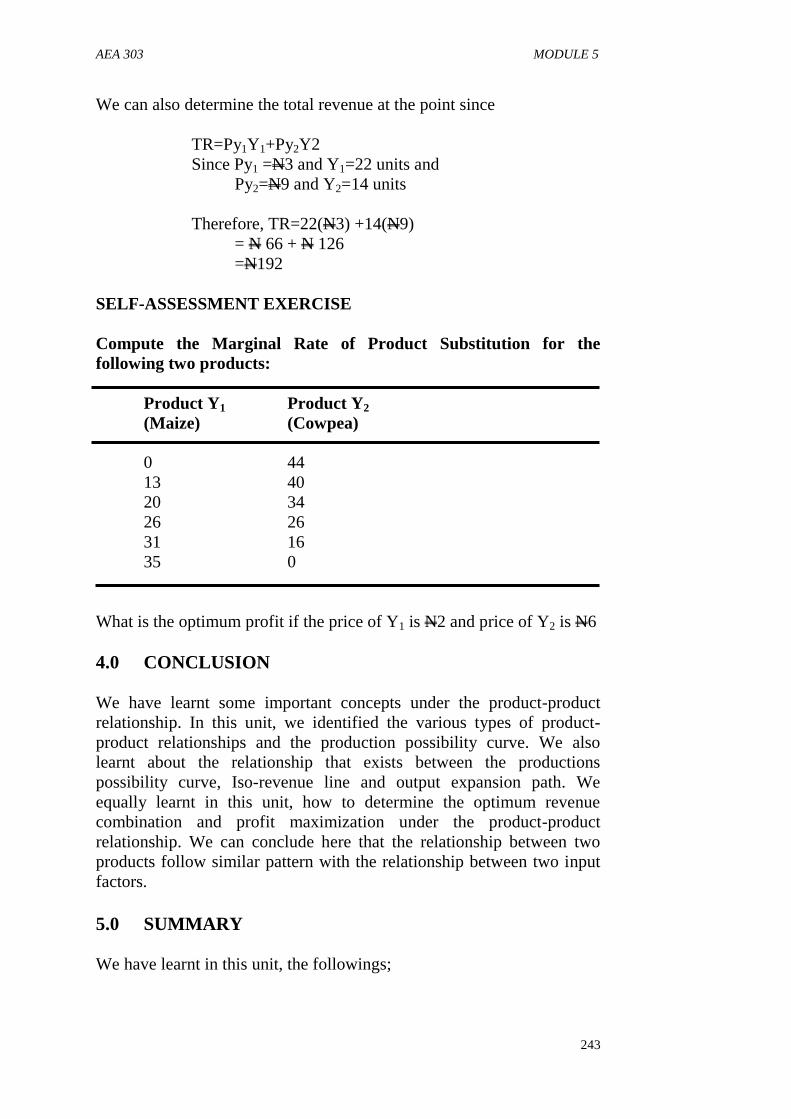
AEA 303 MODULE 5
243
We can also determine the total revenue at the point since
TR=Py1Y1+Py2Y2
Since Py1 =N3 and Y1=22 units and
Py2=N9 and Y2=14 units
Therefore, TR=22(N3) +14(N9)
= N 66 + N 126
=N192
SELF-ASSESSMENT EXERCISE
Compute the Marginal Rate of Product Substitution for the
following two products:
Product Y1 Product Y2
(Maize) (Cowpea)
0 44
13 40
20 34
26 26
31 16
35 0
What is the optimum profit if the price of Y1 is N2 and price of Y2 is N6
4.0 CONCLUSION
We have learnt some important concepts under the product-product
relationship. In this unit, we identified the various types of product-
product relationships and the production possibility curve. We also
learnt about the relationship that exists between the productions
possibility curve, Iso-revenue line and output expansion path. We
equally learnt in this unit, how to determine the optimum revenue
combination and profit maximization under the product-product
relationship. We can conclude here that the relationship between two
products follow similar pattern with the relationship between two input
factors.
5.0 SUMMARY
We have learnt in this unit, the followings;
AEA 303 AGRICULTURAL PRODUCTION ECONOMICS
244
i. Two products can relate together as joint, competitive,
complementary or supplementary
ii. All the four types of product relationships are observed in
agricultural production.
iii. Products are competitive when increase in production of one will
reduce the output of the other one
iv. Two products are joint if increase in the production of one will
increase the output of the other one
v. Two products are said to be complementary if increase or
decrease in the output of one will not affect the output of the
other one
vi. If one input can be used to produce used to produce two products
at different production periods, the two products are said to be
supplementary
vii. If input is fixed, it is possible to have some various combinations
of output from two products. When these combinations are
plotted it is called PPC
viii. It is possible to fix two revenue and then have various
combinations of output of two products. The line joining the two
extremes is called iso-revenue line
ix. Optimum combinations is obtained when MRPS is equated to PR
6.0 TUTOR-MARKED ASSIGNMENT
1. Explain with illustrations the following concepts:
a. Production Possibility Curve
b. Iso-revenue line
c. Output Expansion Path
d. Competitive Product
e. Complementary Product
7.0 REFERENCES/FURTHER READING
Abbot, J.C. and J.P. Makeham (1980). Agricultural Economics and
Marketing in the Tropics. London, Longman Publishers.
Adegeye, A.J. and J.S. Dittoh (1985). Essentials of Agricultural
Economics. Ibadan, Impact Publishers.
Doll, J.P. and Orazen, P. (1978). Production Economics: Theory with
Application. USA, John Willey and Sons Publishers.
Ibitoye, S.J. and Idoko, D. (2009). Principles of Agricultural Economics.
Kaduna. Euneeks and Associates Publishers. Pp 82-92.
AEA 303 MODULE 5
245
Nweze, N.J. (2002). Agricultural Production Economics: An
Introductory Text. Nsukka. AP Express Publishers.
Olayide, S.O. and Heady E.O. (1982). Introduction to Agricultural
Production Economics. Ibadan. University Press Ltd.
Olukosi, J.O. and A.O. Ogungbile (1989). Introduction to Agricultural
Production Economics: Principles and Applications. Zaria.
AGTAB Publishers Ltd.
Marshall A.C. (1998). Modern Farm Management Techniques. Owerri.
Alphabet Nigeria Publishers.
Reddy, S.S., P.R. Ram, T.V. Sastry and I.B. Devi (2004). Agricultural
Economics. New Delhi. Oxford and Ibh Publishers Ltd.
AEA 303 AGRICULTURAL PRODUCTION ECONOMICS
246
MODULE 5 PRODUCTION COSTS
Unit 1 Meaning and Types of Cost
Unit 2 Farm Cost Functions
Unit 3 Cost Functions and Production Function
UNIT 1 MEANING AND TYPES OF COST
CONTENTS
1.0 Introduction
2.0 Objectives
3.0 Main Content
3.1 Meaning of Agricultural Cost
3.2 Types of Cost
3.3 Importance of Cost in Agricultural Production
4.0 Conclusion
5.0 Summary
6.0 Tutor-Marked Assignment
7.0 References/Further Reading
1.0 INTRODUCTION
You are welcome to the last module of this study guide. You will recall
that module 4 was on resource allocation involving both factor-factor
and product-product relationships. We discussed various concepts under
these topics. You can still remember concepts like isoquant, isocost line,
isoclines, ridgeline, expansion path, production possibility curve, iso-
revenue line etc. In this last module, we shall discuss production cost
and in this unit of the module we want to first explain the meaning of
cost, identify the various types of cost and discuss the usefulness of cost.
2.0 OBJECTIVES
At the end of this unit, you should be able to:
define agricultural farm cost
list and explain the meaning of at least four different types of cost
discuss the importance of cost in agricultural production.

AEA 303 MODULE 5
247
3.0 MAIN CONTENT
3.1 Meaning of Agricultural Cost
Agricultural cost according to Ibitoye and Idoko (2009) is referred to as
the value of agricultural output. That is, it is the expenses incurred by
farmers in the process of producing a farm product such as yam, maize,
eggs, goats etc. It is also known as expenses incurred in producing a
particular amount f product in a particular period. Hence one can talk of
the cost of producing 10 tons of yam in a season or 100 litres of milk per
week or 100 crates of eggs per month.
Cost of production can also be referred to as accounting cost, cost of
materials used in the production process such as labour costs, feed costs,
fertilizer costs, maintenance and repair costs, selling and administrative
costs, depreciation costs, taxes and interest payment on money
borrowed.
Agricultural economist view costs of production as embracing a
considerable alternative costs or opportunity costs. For instance, if a
farmer produces only commodity A and no B, the cost of producing A is
the accounting cost plus the forgone return on B known as economic
costs.
3.2 Types of Cost
In considering costs involved in agricultural production, Abbot and
Makeham (1980) indentified five main farm costs. These are variable
costs, overhead costs, financial costs, capital costs and personal costs
3.2.1 Variable Costs
These costs are also known as direct costs. They are the costs which
vary as the size and level of output of farm activities varies. For
example, if the area under maize production is increased by 50%, then
seed, fertilizer, labour inputs etc will also increase but may not be
necessarily at the same rate. It is even possible for input like labour not
to be affected by this increase. Some farm production may have direct
influence on some of their variable costs. For example, if you double the
cattle numbers, variable costs such as feed and veterinary fees will also
double.
Variable costs are directly associated with the level of intensity of each
activity. In a crop production activities for example, crop yield can be

AEA 303 AGRICULTURAL PRODUCTION ECONOMICS
248
influenced by the amount of money invested on variable costs like
fertilizer, seeds, weeding etc.
It is essential for farmers to identify the variable costs of his activities on
the farm such as to give him an idea of the size of the change in cost
which will occur if he expands or contract one or more of his farm
activities. His knowledge of variable costs and probably the gross
income will guide the farmer in making decision on the merit of making
the change on those activities.
Examples of farm variable costs include: seed, fertilizer, animal feed,
agro-chemicals, livestock, seasonal labour, electricity bill, fuel and oil,
machines maintenance and repairs etc.
3.2.2 Overhead Costs
Overhead cost is also known as fixed cost of production. These costs do
not vary with the level of output, which means that they may be incurred
even when production is not undertaking. Thus a small increase or
decrease in the area of crop or number of farm animals is not likely
going to affect the overhead costs of the farm. Examples of farm
overhead costs include: depreciation of plant and equipment, interest on
loan, rental payments for machinery, wages and salaries of permanent
staff, land maintenance and rent etc.
Overhead costs can be either of the following types: Total Overhead
Costs, Operational Costs or Activity Overheads. The total overhead
costs are the unavoidable costs which must be met every year. The total
gross margin is normally the only source other than borrowing, from
which the overhead cost can be met. The essential components of total
overhead costs include the followings: living expenses of the farmer,
wages for permanent staff, loan interest and repayments, taxes, general
repairs, insurance premium, replacement of capital items such as plants,
machinery, building etc, travel and other business expenses.
The operational costs are used in calculating the true profit in accounting
sense. They are overheads associated with annual operational expenses
of the farm. Therefore, such overhead expenses like repayment of loans,
living expenses, interest on loans and income tax are normally excluded
in operational costs. All other costs considered under total overhead
costs are part of operational costs. Some of the costs include: wages of
permanent workers, depreciation charges, operator‟s allowance, general
repairs, insurance charges, telephone and other business expenses.
The third type of overhead cost is the Activity Overheads. This type of
overheads are those costs which would not be incurred if the business
operation was terminated. Such cost includes depreciation charges on
equipment.

AEA 303 MODULE 5
249
AEA 303 AGRICULTURAL PRODUCTION ECONOMICS
250
3.2.3 Finance Costs
These costs are associated with loan repayment and insurance costs and
interest paid on loan.
3.2.4 Capital Costs
These costs are usually associated with costs incurred in the process of
providing capital assets used in farm production. Examples of capital
costs include costs on land clearing, land purchase, machinery, building,
plantation and livestock establishment.
3.2.5 Personal Costs
The living or personal costs of the farmer are normally included in the
total overhead costs. Personal costs are one of the most important and
unavoidable items in the total farm overheads. Personal costs on the
farm include costs of food items, clothing, medical expenses, school
fees, costs of traveling etc. some of these personal costs items are
directly related to the level of output of the farmer.
3.3 Importance of Cost in Agricultural Production
One of the major motives of any farmer is profit maximization. Profit is
obtained by subtracting total cost from total revenue (π = TR – TC). It is
important therefore, for farmers to understand the nature and structure of
production costs and how they affect the decision making process.
Understanding of cost functions also help farmers to determine the most
profitable level of production as well as the level of output in which
production process depends. Cost functions also help to determine the
least cost combination (cost minimization) that will determine maximum
profit.
Cost functions also help the farmer to determine how much variable
factor to be employed in combination with fixed factors in the
production of an output for maximum benefit.
SELF-ASSESSMENT EXERCISE
i. Differentiate between variable, overhead, personal, finance and
capital costs. Give examples in each case.
ii. Itemize three relevance of cost to a farmer.

AEA 303 MODULE 5
251

AEA 303 AGRICULTURAL PRODUCTION ECONOMICS
252
4.0 CONCLUSION
In this unit, we discussed the meaning and the different types of farm
cost. We learnt about variable cost, overhead costs, financial costs,
capital costs and personal costs. We also concluded that without the
knowledge of farm costs it will be impossible to determine farm profit.
5.0 SUMMARY
The main points discussed in this unit include the followings:
i. agricultural costs are the value of inputs used on the farm
ii. there are five major categories of costs- variable, overhead,
financial, capital and personal costs
iii. variable cost is also called direct costs and are the costs which
vary according to the level of output
iv. overhead costs also called fixed costs are costs that must be
incurred even when there is no production
v. overhead costs can be categorized into total overhead cost,
operational costs and activity costs
vi. loan repayment, insurance premium and interest on loan
constitute fiancé cost
vii. all costs incurred while providing capital assets are categorized as
capital costs
viii. cost of living incurred outside the farm are classified as personal
costs e.g. food, clothing, school fees, medicals, travels etc
ix. costs enable farmers to calculate their profit on the farm
6.0 TUTOR-MARKED ASSIGNMENT
1 (a). What is Agricultural Cost?
(b). What is the implication of cost to a farmer?
7.0 REFERENCES/FURTHER READING
Abbot, J.C. and J.P. Makeham (1980). Agricultural Economics and
Marketing in the Tropics. London, Longman Publishers.
Adegeye, A.J. and J.S. Dittoh (1985). Essentials of Agricultural
Economics. Ibadan, Impact Publishers.
Ibitoye, S.J. and Idoko, D. (2009). Principles of Agricultural Economics.
Kaduna. Euneeks and Associates Publishers. Pp 82-92.
AEA 303 MODULE 5
253
Nweze, N.J. (2002). Agricultural Production Economics: An
Introductory Text. Nsukka. AP Express Publishers.
Olayide, S.O. and Heady E.O. (1982). Introduction to Agricultural
Production Economics. Ibadan. University Press Ltd.
Olukosi, J.O. and A.O. Ogungbile (1989). Introduction to Agricultural
Production Economics: Principles and Applications. Zaria.
AGTAB Publishers Ltd.
Marshall A.C. (1998). Modern Farm Management Techniques. Owerri.
Alphabet Nigeria Publishers.
Reddy, S.S., P.R. Ram, T.V. Sastry and I.B. Devi (2004). Agricultural
Economics. New Delhi. Oxford and Ibh Publishers Ltd.

AEA 303 AGRICULTURAL PRODUCTION ECONOMICS
254
UNIT 2 FARM COST FUNCTIONS
CONTENTS
1.0 Introduction
2.0 Objectives
3.0 Main Contents
3.1 Classical Measures of Cost
3.2 Short Run Cost and Long Run Cost
3.3 Agricultural Cost Functions
4.0 Conclusion
5.0 Tutor-Marked Assignment
6.0 References/Further Reading
1.0 INTRODUCTION
Unit 1 of this module focused attention on the meaning and types of
farm cost. By now you should be familiar with the definition of farm
cost, different types of cost associated with agricultural production and
the importance of costs to a farmer. In this unit we shall explain some
cost concepts like total cost, variable cost, fixed cost, average total cost,
average variable cost, average fixed cost and marginal cost. We shall try
to distinguish between short run and long run costs.
2.0 OBJECTIVES
At the end of this unit, you should be able to:
explain the meaning of Total Costs (TC)
calculate Average Total Cost (ATC), Average variable Cost
(AVC) and Average Fixed Cost (AFC)
calculate the Marginal Cost (MC) of farm operations
differentiate between short run cost and long run cost
tabulate and plot the graph of agricultural cost functions
3.0 MAIN CONTENTS
3.1 Classical Measures of Cost
The classical approach to cost measurement include: Total Cost,
Variable Cost, Fixed Cost and Marginal Cost Functions.

AEA 303 MODULE 5
255
3.1.1 Total Cost (TC)
Total Cost (TC) of production is the total outlay on a given output level.
Total cost is given as Fixed Cost (FC) plus Variable Cost (VC). i.e.
TC = FC + VC
Average Total Cost (ATC) or Average Cost (AC) is obtained by
dividing Total Cost by output.
Total Costs (TC) TC TFC TVC
TFC + TVC
ATC = = = + =
Output (Y) Y Y Y
Y
Therefore, ATC = AFC + AVC
3.1.2 Fixed Costs (FC)
Fixed costs are the costs of production which remains constant
irrespective of change in output level. In the short run FC remains the
same irrespective of the level of production but in the long run there are
no fixed costs. Fixed cost is also known as overhead cost, indirect cost
or sunk cost. When plotted on the graph, it is a horizontal straight line
parallel to the x-axis.
Average Fixed Cost (AFC) is measured by this formula:
AFC = Total Fixed Cost = TFC
Output Y
It is the cost of fixed input required for producing one unit of output.
Therefore, AFC decreases as output level increases.
Mathematically, since ATC = AFC + AVC
Therefore, AFC = ATC AVC
3.1.3 Total Variable Cost (TVC)
Total Variable Costs (TVC) of production are those costs associated
with production process which varies in size positively with variations
in output level. This means that TVC increases with increase in output
vice versa and is zero when there is no production at all.
When TFC is deducted from TC what left is TVC.
Average Variable Cost (AVC) is equal to TVC divided by output.
That is AVC = TVC/Y
It is the TVC per unit of output (Y).

AEA 303 AGRICULTURAL PRODUCTION ECONOMICS
256
AVC = ATC AFC
The relationship between TVC and output shows that when small
amount of output is produced, cost of variable input per unit of output
becomes very high. As more of the variable inputs are used in the
production process, productivity of the variable inputs will increase due
to economies of scale.
3.1.4 Marginal Cost (MC)
The Marginal Cost is the increase in Total Cost (TC) resulting from
increasing the output by one unit. It is also known as incremental cost.
MC = Change in TC = ΔTC
Change in output ΔY
The only component that changes in Total Cost is the TVC. We can
therefore use either TC or TVC to compute the MC.
MC = ΔTC = ΔFC + ΔVC
ΔY ΔY ΔY
But ΔFC = 0, therefore MC = ΔVC
ΔY ΔY
The relationship between output (Y) and Total Cost (TC), Total variable
Cost (TVC), Total Fixed Cost (TFC) and Marginal Cost (MC) can be
presented in a tabular form.
Table 7: The Relationship between TC, TVC, TFC, MC and Output of
Commodity
Output TFC TVC TC AFC AVC ATC MC
0 100 0 100 - - - -
1 100 40 140 100 40 140 40
2 100 64 164 50 32 82 24
3 100 80 180 33.3 26.7 60 16
4 100 88 188 25 22 47 8
5 100 96 196 20 19.2 39.2 8
3.2 Short Run and Long Run Costs
In the short run, we can classify Total Cost into fixed cost and variable
cost. Therefore all the classical measures of costs considered above
occur in the short run.
In the long run, all costs can be varied because all inputs can increase or
decrease with the level of output. The implication of this in cost function
is that in the long run the relevant cost concepts are the total cost and
marginal cost. Therefore, marginal cost in the long run cost is the rate of

AEA 303 MODULE 5
257
change in total cost with respect to changes in output. The issue of
variable cost is no longer relevant here.
Algebraically,
Long Run Average Cost (LAC) = LTC and LMC = ΔLTC
Y ΔY
The relationships which exist among the LTC, LAC and LMC are the
same as in the short run TC, AC and MC. Some of these relationships
will be considered under the agricultural cost functions.
3.3 Agricultural Cost Functions
Marshal (1998) defined agricultural cost function as the relationship
between agricultural production costs and output. Agricultural cost
functions are derived from production functions in terms of the number
of variable inputs used in the production process. Thus it is possible to
have agricultural cost functions with one, two or more variable inputs.
Our illustration here will be based on cost functions with just one
variable input. Here we shall illustrate the production costs for various
levels of output with the production function with one variable thus:
Y = ƒ(X)
The cost function for the above implicit production function can be
written as:
Y = ƒ(PxX)
Where Y = Variable cost of input X
X = Variable input
Px = Price of the input X
Various cost functions exist within a production function with one
variable input, such functions include: Total Cost, Fixed Cost, variable
Cost and Marginal Cost. We have already considered the meaning and
measures of these costs.
We shall first consider the relationships between Total Cost (TC), Total
Fixed Cost (TFC) and Total Variable Cost (TVC).
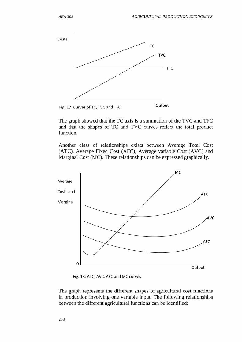
AEA 303 AGRICULTURAL PRODUCTION ECONOMICS
258
The graph showed that the TC axis is a summation of the TVC and TFC
and that the shapes of TC and TVC curves reflect the total product
function.
Another class of relationships exists between Average Total Cost
(ATC), Average Fixed Cost (AFC), Average variable Cost (AVC) and
Marginal Cost (MC). These relationships can be expressed graphically.
The graph represents the different shapes of agricultural cost functions
in production involving one variable input. The following relationships
between the different agricultural functions can be identified:
Fig. 17: Curves of TC, TVC and TFC
Costs
Output
TC
TVC
TFC
MC
ATC
AFC
AVC
Output 0
Average
Costs and
Marginal
Cost
Fig. 18: ATC, AVC, AFC and MC curves

AEA 303 MODULE 5
259
i. When ATC and AVC are at their maximum points, MC and ATC
are equal. MC and AVC are also equal.
ii. MC and ATC are equal at an output level that is greater than the
output level at which MC equals AVC
iii. AFC slopes downward from left to right and asymptotically
approach the output axis as output increases
iv. The slope of ATC becomes zero at the minimum point of ATC
and MC equals ATC at that point.
SELF-ASSESSMENT EXERCISE
Calculate the AFC, AVC, ATC and MC for each level of output from
the following total cost data:
Input (X) Output (Y) Total Cost (N)
0 0 100
1 4 200
2 9 300
3 15 400
4 21 500
5 26 600
6 32 700
7 35 800
8 36 900
9 35 1000
10 30 1100
4.0 CONCLUSION
In this unit, we focused our attention on farm cost functions. We
discussed how to measure the different types of costs such as Total Cost,
Fixed Cost, Variable Cost and Marginal Cost. We also differentiated
between short run and long run costs. We concluded this unit by
expressing the farm costs functions in tabular and graphical forms.
5.0 SUMMARY
The main points discussed in this unit include the followings:
i. Total Cost (TC) = Total Fixed Cost (TFC) + Total Variable Cost
(TVC)
ii. Average Total Cost (ATC) = Total Cost (TC)
Output (Y)
iii. Fixed costs are the costs which do not vary with output
iv. Average Fixed Cost (AFC) = Total Fixed Cost (TFC)
Output (Y)

AEA 303 AGRICULTURAL PRODUCTION ECONOMICS
260
v. Total Variable Costs (TVC) are those costs which vary with
output
vi. Average Variable Cost (AVC) = Total Variable Cost (TFC)
Output (Y)
vii. Marginal Cost (MC ) = Change in TC = ΔTC
Change in Y ΔY
viii. Fixed cost and variable cost in short run costs are not relevant in
long run costs.
ix. The measures of TC, AC and MC in the short run costs are the
same as in LTC, LAC and LMC
x. When ATC and AVC are at the minimum points, MC and ATC
and MC and AVC are equal.
6.0 TUTOR-MARKED ASSIGNMENT
Discuss the classical measures of the following farm cost functions:
Total Cost, Fixed Cost, Variable Cost and Marginal Cost.
7.0 REFERENCES/FURTHER READING
Abbot, J.C. and J.P. Makeham (1980). Agricultural Economics and
Marketing in the Tropics. London, Longman Publishers.
Adegeye, A.J. and J.S. Dittoh (1985). Essentials of Agricultural
Economics. Ibadan, Impact Publishers.
Doll, J.P. and Orazen, P. (1978). Production Economics: Theory with
Application. USA, John Willey and Sons Publishers.
Ibitoye, S.J. and Idoko, D. (2009). Principles of Agricultural Economics.
Kaduna. Euneeks and Associates Publishers. Pp 82-92.
Nweze, N.J. (2002). Agricultural Production Economics: An
Introductory Text. Nsukka. AP Express Publishers.
Olayide, S.O. and Heady E.O. (1982). Introduction to Agricultural
Production Economics. Ibadan. University Press Ltd.
Olukosi, J.O. and A.O. Ogungbile (1989). Introduction to Agricultural
Production Economics: Principles and Applications. Zaria.
AGTAB Publishers Ltd.
Marshall A.C. (1998). Modern Farm Management Techniques. Owerri.
Alphabet Nigeria Publishers.
Reddy, S.S., P.R. Ram, T.V. Sastry and I.B. Devi (2004). Agricultural
Economics. New Delhi. Oxford and Ibh Publishers Ltd.
AEA 303 MODULE 5
261
UNIT 3 COST FUNCTIONS AND PRODUCTION
FUNCTION
CONTENTS
1.0 Introduction
2.0 Objectives
3.0 Main contents
3.1 Relationship Between Cost Curves and Production
function
3.2 Relationships Between APP and MPP Curves and AC and
MC curves
3.3 Total Revenue and Cost Functions
4.0 Conclusion
5.0 Summary
6.0 Tutor-Marked Assignment
7.0 Reference/Further Reading
1.0 INTRODUCTION
In the last unit we discussed farm functions. In the unit we looked at
how we can measure total cost, fixed cost, variable cost and marginal
cost. In that unit we differentiated between short run and long run costs
and we graphically illustrated the relationships between ATC, AVC and
MC curves. In this last unit we shall look at the relationships between
cost functions and production function. This comparison will be done
with the aid of tables and graphs.
2.0 OBJECTICVES
At the end of this unit, you should be able to:
explain the relationship between cost curves and production
function
explain the relationships between APP and MPP curves and AC
and MC curves
express total value product in tabular and graphical forms

AEA 303 AGRICULTURAL PRODUCTION ECONOMICS
262
3.0 MAIN CONTENTS
3.1 Relationships between Cost Curves and Production
Function
We have already discussed the components of cost functions under the
short run. In the short run, Total cost comprised of Total Variable Cost
and Total Fixed Cost.
The case of one variable input can be expressed as
TC=TVC+TFC
=PXX+A
Where PX= price of input
X=variable input
A=Total Fixed Cost
Similarly, production function (PF) expressed the relationship between
input and output.
The case of one variable input and one output can be expressed as
Y=a+bX
Where
Y=output
X=input
b=coefficient
a=constant
The two functions as expressed above involved input (X).
The production function expressed output as a function of input and
costs are also involved in this production. There can be no production
without cost.
The level of cost determines the level of production. The knowledge of
input price (PX) allows the determination and analyzes of the
relationship between the two functions. The graphical expression of cost
functions and production function will give a clearer picture of the
relationships.

AEA 303 MODULE 5
263
The total cost functions comprised of Total Cost (TC), Total Variable
Cost (TVC) and Total Fixed Cost (TFC) curves. Output (Y) is expressed
on the Y-axis of PF and on the X-axis of cost functions. The TC and
TVC have the same shape and the gap between the two is a result of
TFC. The graph shows an inverse relationship between PF and TC and
TVC curves. This indicates that where Total Product (TP) is increasing
at an increasing rate, the TC and TVC will increase at a decreasing rate
and vice versa.
3.1 Relationship Between Average Product and Average
Cost Curves and Marginal Product and Marginal Cost
Curves
3.1.1 Average Product and Average Cost Curves
Average Product (AP) curve is derived from production function while
Average Cost (AC) is derived from cost function. The relationship
between these two functions can be expressed both graphically and
algebraically just as in the case of production function and cost function.
Fig. 19: Production Function Fig. 20: Cost Functions
Output(Y)
COST
Output
(Y)
Input
(x)
TFC
TVC
TC

AEA 303 AGRICULTURAL PRODUCTION ECONOMICS
264
Fig. 21: Average Physical Product Curve Fig. 22: Average Variable Cost Curve
Just as we established in the case of PF and TC, there is also an inverse
relationship between APP and AVC. As APP is increasing, AVC is
decreasing. This relationship can also be expressed in algebraic form
APP = Total Output = Y …..…………… (1)
Total Input X
and
AVC = Total Variable Cost = TVC …..………… (2)
Total Output Y
TVC = Px Y
Therefore, AVC = Px Y …………………………………….. (3)
Y
X in AVC is an inverse of Y in APP
Y X
We can therefore rewrite equation (3) as
AVC = PX . 1 = Px
APP APP …………………………… (4)
Equation (4) therefore confirms the inverse relationship between APP
and AVC.
AVC
Output (Y) Input (x)
Output
(Y)
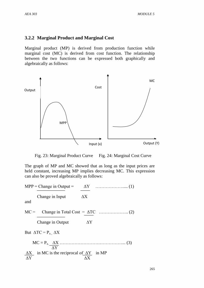
AEA 303 MODULE 5
265
3.2.2 Marginal Product and Marginal Cost
Marginal product (MP) is derived from production function while
marginal cost (MC) is derived from cost function. The relationship
between the two functions can be expressed both graphically and
algebraically as follows:
Fig. 23: Marginal Product Curve Fig. 24: Marginal Cost Curve
The graph of MP and MC showed that as long as the input prices are
held constant, increasing MP implies decreasing MC. This expression
can also be proved algebraically as follows:
MPP = Change in Output = ΔY ………………..... (1)
Change in Input ΔX
and
MC = Change in Total Cost = ΔTC ……………….. (2)
Change in Output ΔY
But ΔTC = Px , ΔX
MC = Px. ΔX ……………………………………... (3)
ΔY
ΔX in MC is the reciprocal of ΔY in MP
ΔY ΔX
MPP
MC
Output (Y)
Cost
N
Output
(Y)
Input (x)

AEA 303 AGRICULTURAL PRODUCTION ECONOMICS
266
We can then rewrite equation (3) as follows:
MC = PX . 1 = PX ………………………………..(4)
MMP MPP
This equation (4) confirm our graphical expression that as long as the
price of input is constant, increasing the MC will implies decreasing MP
and vice versa.
3.3 Total Revenue and Cost Functions
Total Revenue (TR) or Total Value Product (TVP) is the monetary value
of the output
i.e. TR = Py .Y
Where
Py = Price per unit of output
Y = Total Output.
We can deduce from here that
TR or TVP is related to output (Py . Y) and we have already established
that TC is related to input (Px . X). We can then conclude that production
function relates input to TR and also output to TC.
This relationship can be illustrated further in a tabular form:
Table 13: Revenue and Cost of a Farm
Output
(Y)
1
TC
(TVC
+
TFC)
2
Price
or AR
3
TR
(Py.Y)
4
ATC
(3 x
1)
5
MC
Δin2
Δin1
6
MR
Δin4
Δin1
7
NR
(4 –
2)
8
0
10 20 0 - - - 10
1 122 20 20 12.0 2 20 8
2 14 20 40 7.0 2 20 26
3 16 20 60 5.3 2 20 34
4 18 20 80 4.5 2 20 62
5 20 20 100 4.0 2 20 80
SELF-ASSESSMENT EXERCISE

AEA 303 MODULE 5
267
Differentiate between Average Product (AP) and Average Cost (AC)
using graphical and algebraic expressions for both production and cost
functions.
4.0 CONCLUSION
In this unit, we discussed the relationships between cost functions and
production function. We showed the relationships between TC and TVC
functions and total physical product function. In this unit we also
discussed the relationships between average product and average cost
curves and marginal product and marginal cost curves. We equally relate
total revenue function to cost function. We can then conclude that
production function serves as linkage between the cost functions and
total revenue functions.
5.0 SUMMARY
The main points in this unit include the followings:
i. There are inverse relationships between production function and
cost functions
ii. Where PF is increasing at an increasing rate, TC and TVC are
increasing at a decreasing rate.
iii. Average Product (AP) is also inversely related to Average
Variable Cost (AVC).
AVC = Px /APP
iv. Similarly Marginal Product (MP) is inversely related to Marginal
Cost (MC)
MC = Px . 1
MPP
v. TR is related to output, TC is related to input and PF relates input
to output. Therefore PF serves as linkage between TR and TC.
6.0 TUTOR-MARKED ASSIGNMENT
1. From the table below, find the values of Marginal Revenue and
Marginal Cost
Output of Total Revenue Total Cost
Beans (Kg) (N) N
10 150 250
20 200 300
30 350 430
40 450 500
50 550 550

AEA 303 AGRICULTURAL PRODUCTION ECONOMICS
268
60 600 580
70 630 700

AEA 303 MODULE 5
269
7.0 REFERENCES/FURTHER READING
Abbot, J.C. and J.P. Makeham (1980). Agricultural Economics and
Marketing in the Tropics. London, Longman Publishers.
Adegeye, A.J. and J.S. Dittoh (1985). Essentials of Agricultural
Economics. Ibadan, Impact Publishers.
Doll, J.P. and Orazen, P. (1978). Production Economics: Theory with
Application. USA, John Willey and Sons Publishers.
Ibitoye, S.J. and Idoko, D. (2009). Principles of Agricultural Economics.
Kaduna. Euneeks and Associates Publishers. Pp 82-92.
Nweze, N.J. (2002). Agricultural Production Economics: An
Introductory Text. Nsukka. AP Express Publishers.
Olayide, S.O. and Heady E.O. (1982). Introduction to Agricultural
Production Economics. Ibadan. University Press Ltd.
Olukosi, J.O. and A.O. Ogungbile (1989). Introduction to Agricultural
Production Economics: Principles and Applications. Zaria.
AGTAB Publishers Ltd.
Marshall A.C. (1998). Modern Farm Management Techniques. Owerri.
Alphabet Nigeria Publishers.
Reddy, S.S., P.R. Ram, T.V. Sastry and I.B. Devi (2004). Agricultural
Economics. New Delhi. Oxford and Ibh Publishers Ltd.