Adversarial topology discovery in network virtualization environments: a threat for ISPs?

Distrib. Comput.DOI 10.1007/s00446-014-0217-4

Adversarial topology discovery in network virtualizationenvironments: a threat for ISPs?

Yvonne Anne Pignolet · Stefan Schmid · Gilles Tredan

Received: 23 April 2013 / Accepted: 9 April 2014© Springer-Verlag Berlin Heidelberg 2014

Abstract Network virtualization is a new Internet para-digm which allows multiple virtual networks (VNets) to sharethe resources of a given physical infrastructure. The virtual-ization of entire networks is the natural next step after thevirtualization of nodes and links. While the problem of howto embed a VNet (“guest network”) on a given resource net-work (“host network”) is algorithmically well-understood,much less is known about the security implications of thisnew technology. This paper introduces a new model to rea-son about one particular security threat: the leakage of infor-mation about the physical infrastructure—often a businesssecret. We initiate the study of this new problem and intro-duce the notion of request complexity which describes thenumber of VNet requests needed to fully disclose the sub-strate topology. We derive lower bounds and present algo-rithms achieving an asymptotically optimal request complex-ity for important graph classes such as trees, cactus graphs(complexity O(n)) as well as arbitrary graphs (complexityO(n2)). Moreover, a general motif-based topology discoveryframework is described which exploits the poset structure ofthe VNet embedding relation.

This article is based on the conference publications [20–22].

Y. A. PignoletABB Corporate Research, Dättwil, Switzerlande-mail: [email protected]

S. Schmid (B)Telekom Innovation Laboratories and TU Berlin, Berlin, Germanye-mail: [email protected]

G. TredanLAAS-CNRS, Toulouse, Francee-mail: [email protected]

1 Introduction

Virtualization is arguably the main innovation motor intoday’s Internet. Already a decade ago, node virtualiza-tion revamped the server business, and today’s datacentershost thousands of virtual machines. But also links becomemore virtualized, e.g., through the introduction of Software-Defined Networking [19] technology.

After the virtualization of nodes and links, the industryas well as the academia discusses the virtualization of entirenetworks: network virtualization [8,15] envisions an Internetwhere customers (e.g., a startup company or a content dis-tribution provider) can request virtual networks (VNets) onshort notice and with arbitrary specifications on the requirednode resources and their connectivity. Indeed, first prototypeshave emerged (e.g., in the European CHANGE and UNIFYprojects, the American GENI project or the Asian AKARIproject). Network virtualization is particularly attractive forInternet Service Providers (ISPs): ISPs benefit from theimproved resource utilization as well as from the possibil-ity to introduce new services [27].

This paper argues that the network virtualization trend alsocomes with certain threats. In particular, we show that crit-ical information about the ISP’s network infrastructure andits properties can be learned from answers to VNet embed-ding requests. Given that the resource network constitutes acompetitive advantage and is a business secret, this is prob-lematic; moreover, the discovery of, e.g., bottlenecks, maybe exploited for attacks or bad publicity. Hence, providersaround the world are often reluctant to open the infrastruc-ture to novel technologies and applications that might leadto information leaks.Background on VNets and embeddings Basically, a VNetdefines a graph (henceforth: the guest graph): a set of vir-tual nodes (e.g., virtual machines) which need to be intercon-

123

Y. A. Pignolet et al.

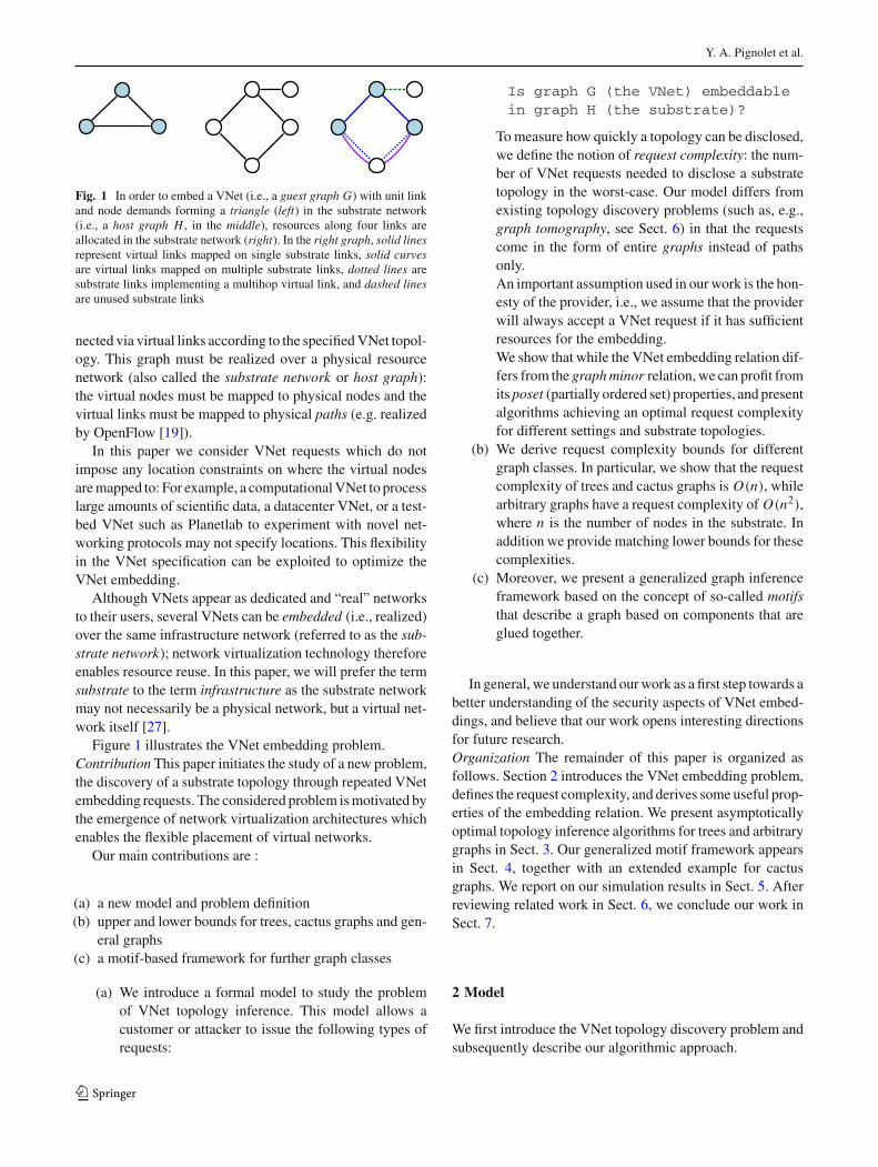
Fig. 1 In order to embed a VNet (i.e., a guest graph G) with unit linkand node demands forming a triangle (left) in the substrate network(i.e., a host graph H , in the middle), resources along four links areallocated in the substrate network (right). In the right graph, solid linesrepresent virtual links mapped on single substrate links, solid curvesare virtual links mapped on multiple substrate links, dotted lines aresubstrate links implementing a multihop virtual link, and dashed linesare unused substrate links

nected via virtual links according to the specified VNet topol-ogy. This graph must be realized over a physical resourcenetwork (also called the substrate network or host graph):the virtual nodes must be mapped to physical nodes and thevirtual links must be mapped to physical paths (e.g. realizedby OpenFlow [19]).

In this paper we consider VNet requests which do notimpose any location constraints on where the virtual nodesare mapped to: For example, a computational VNet to processlarge amounts of scientific data, a datacenter VNet, or a test-bed VNet such as Planetlab to experiment with novel net-working protocols may not specify locations. This flexibilityin the VNet specification can be exploited to optimize theVNet embedding.

Although VNets appear as dedicated and “real” networksto their users, several VNets can be embedded (i.e., realized)over the same infrastructure network (referred to as the sub-strate network); network virtualization technology thereforeenables resource reuse. In this paper, we will prefer the termsubstrate to the term infrastructure as the substrate networkmay not necessarily be a physical network, but a virtual net-work itself [27].

Figure 1 illustrates the VNet embedding problem.Contribution This paper initiates the study of a new problem,the discovery of a substrate topology through repeated VNetembedding requests. The considered problem is motivated bythe emergence of network virtualization architectures whichenables the flexible placement of virtual networks.

Our main contributions are :

(a) a new model and problem definition(b) upper and lower bounds for trees, cactus graphs and gen-

eral graphs(c) a motif-based framework for further graph classes

(a) We introduce a formal model to study the problemof VNet topology inference. This model allows acustomer or attacker to issue the following types ofrequests:

Is graph G (the VNet) embeddablein graph H (the substrate)?

To measure how quickly a topology can be disclosed,we define the notion of request complexity: the num-ber of VNet requests needed to disclose a substratetopology in the worst-case. Our model differs fromexisting topology discovery problems (such as, e.g.,graph tomography, see Sect. 6) in that the requestscome in the form of entire graphs instead of pathsonly.An important assumption used in our work is the hon-esty of the provider, i.e., we assume that the providerwill always accept a VNet request if it has sufficientresources for the embedding.We show that while the VNet embedding relation dif-fers from the graph minor relation, we can profit fromits poset (partially ordered set) properties, and presentalgorithms achieving an optimal request complexityfor different settings and substrate topologies.

(b) We derive request complexity bounds for differentgraph classes. In particular, we show that the requestcomplexity of trees and cactus graphs is O(n), whilearbitrary graphs have a request complexity of O(n2),where n is the number of nodes in the substrate. Inaddition we provide matching lower bounds for thesecomplexities.

(c) Moreover, we present a generalized graph inferenceframework based on the concept of so-called motifsthat describe a graph based on components that areglued together.

In general, we understand our work as a first step towards abetter understanding of the security aspects of VNet embed-dings, and believe that our work opens interesting directionsfor future research.Organization The remainder of this paper is organized asfollows. Section 2 introduces the VNet embedding problem,defines the request complexity, and derives some useful prop-erties of the embedding relation. We present asymptoticallyoptimal topology inference algorithms for trees and arbitrarygraphs in Sect. 3. Our generalized motif framework appearsin Sect. 4, together with an extended example for cactusgraphs. We report on our simulation results in Sect. 5. Afterreviewing related work in Sect. 6, we conclude our work inSect. 7.

2 Model

We first introduce the VNet topology discovery problem andsubsequently describe our algorithmic approach.

123

Network virtualization environments

2.1 VNet embedding

Our formal setting consists of two entities: a customer (the“adversary”) that issues virtual network (VNet) requests anda provider (a virtual network or infrastructure provider [27])that performs the access control and the embedding of VNets.We model the virtual network requests as simple, undirectedgraphs G = (V, E, w) (the so-called guest graphs) where Vdenotes the virtual nodes, E denotes the virtual edges con-necting nodes in V , and w denotes the resource requirementsof the node resp. link: the weight w(v) describes the demandof node v ∈ V for, e.g., computation or storage, and w(e)describes the bandwidth demand of edge e ∈ E . Similarly,the infrastructure network is given as an undirected graphH = (V, E, w) (the so-called host graph or substrate) aswell, where V denotes the set of substrate nodes and E isthe set of substrate links. Again, a weight function w candescribe the available resources on a given node or edge.

Without loss of generality, we assume that neither theVNet nor the substrate topologies contain parallel edges orself-loops, and that H is connected. (As we will see, if Hconsists of multiple connected components, these compo-nents can be processed sequentially with our algorithms bykeeping the VNet embedding in an already discovered com-ponent in order to focus on the next component.) Moreover,in this paper, in order to focus on the topological aspects, wewill typically consider host graphs with unit capacities only,i.e., we will assume that w ≡ 1. As we will see, for substratenetworks with unit capacities, we can also make the guestgraph unweighted: all graph classes considered in this papercan be inferred with an asymptotically optimal complexityusing unweighted VNets only.

In this paper we assume that besides the resource demands,the VNet requests do not impose any mapping restrictions,i.e., a virtual node can be mapped to any substrate node,and we assume that a virtual link connecting two substratenodes can be mapped to an entire (but single) path on thesubstrate as long as the demanded capacity is available. Theseassumptions are common for virtual networks [8].

A virtual link which is mapped to more than one substratelink however can entail certain costs at the relay nodes, thesubstrate nodes which do not constitute endpoints of the vir-tual link and merely serve for forwarding. For example, thiscost may represent a header lookup cost and may be a func-tion of the packet rate. However, depending on the appli-cation, the cost can also be more complex, e.g., in case of aVNet which requires additional functionality at the backbonerouters, e.g., to implement an intrusion detection system. Wemodel these kinds of costs with a parameter ε > 0 (per link).Moreover, we also allow multiple virtual nodes to be mappedto the same substrate node if the node capacity allows it; weassume that if two virtual nodes are mapped to the same sub-strate node, the cost of a virtual link between them is zero.

Armed with these definitions, we can formalize our VNetembedding problem.

Definition 1 (Embedding π , Validity Properties, Embed-ding Relation �→) An embedding of a graph A=(VA, E A, wA)

to a graph B = (VB, EB, wB) is a mapping π : A → Bwhere every node of A is mapped to exactly one node of B,and every edge of A is mapped to a path of B. That is, π con-sists of a node mapping πV : VA → VB and an edge mappingπE : E A → PB , where PB denotes the set of paths. We willrefer to the set of virtual nodes embedded on a node vB ∈ VB

by π−1V (vB); similarly, π−1

E (eB) describes the set of virtuallinks passing through eB ∈ EB and π−1

E (vB) describes thevirtual links passing through vB ∈ VB with vB serving as arelay node.

To be valid, the embedding π has to fulfill the follow-ing four properties: (i) Each node vA ∈ VA is mapped toexactly one node vB ∈ VB (but given sufficient capaci-ties, vB can host multiple nodes from VA). (i i) Links aremapped consistently, i.e., for two nodes vA, v′

A ∈ VA, ifeA = {vA, v′

A} ∈ E A then eA is mapped to a single (possiblyempty and undirected) path in B connecting nodes π(vA)

and π(v′A). A link eA cannot be split into multiple paths.

(i i i) The capacities of substrate nodes are not exceeded: forall vB ∈ VB : ∑

u∈π−1V (vB )

w(u) + ε · |π−1E (vB)| ≤ w(vB).

(iv) The capacities in EB are respected as well, i.e., for alleB ∈ EB : ∑

e∈π−1E (eB )

w(e) ≤ w(eB).If there exists such a valid embedding π , we say that graph

A can be embedded in B, indicated by A �→ B. Hence, �→denotes the VNet embedding relation.

Definition 2 (Embedding Cost) The cost associated with anembedding π is denoted by

Cost(π) =∑

vA∈VA

w(vA) +∑

eA∈E A

w(eA) · |π−1(eA)|

+ ε ·∑

vB∈VB

|π−1E (vB)|

The provider has a flexible choice where to embed a VNetas long as a valid mapping is chosen. In order to design topol-ogy discovery algorithms, we can exploit the poset propertyof the embedding relation. The proof of the following lemmaappears in the “Appendix”.

Lemma 1 The embedding relation �→ applied to any graphfamily G (short: (G, �→)), forms a partially ordered set (aposet), i.e., it satisfies reflexivity, antisymmetry and transitiv-ity.

Observe that even though the VNet embedding is similarto the minor graph relation, there are some important dif-ferences. The following lemma shows that the minor graphrelation and the embedding relation do not imply each other.The proof appears in the “Appendix”.

123


Lemma 2 Given two graphs A, B ∈ G with unit capacityit holds that (i) A �→ B implies that A is a minor of B forε > 0.5. (i i ) For smaller ε it holds that A may be embeddablein B even if A is not a minor of B. (i i i ) Not every minor Aof a graph B can be embedded in A.

2.2 Request complexity

We assume the perspective of a customer (an “adversary”)that seeks to disclose the (fixed) infrastructure topology of aprovider with a minimal number of requests. These requests(and the answers to them) are the only means of obtain-ing information. As a performance measure, we introducethe notion of request complexity, i.e., the number of VNetrequests which have to be issued until a given network isfully discovered, i.e., all vertices, edges and capacities areknown to the adversary. The motivation for focusing on arequest measure is based on the fact that a request consti-tutes the natural unit of negotiation between customer andprovider, and issuing a request entails a certain overhead forboth sides. In particular a situation where after the provider’sanswers, the customer repeatedly revokes her request, can beperceived as a denial-of-service attack. Algorithms achievinga low request complexity hence also ensure that adversarialinformation discovery activities remain hidden.

We are interested in algorithms that “guess” the targettopology H (the host graph) among the set H of possiblesubstrate topologies allowed by the model. Concretely, weassume that given a VNet request G (a guest graph), thesubstrate provider always responds with an honest (binary)reply R informing the customer whether the requested VNetG is embeddedable on the substrate H . In the following, wewill use the notation

request(G, H)

to denote such an embedding request of G to H , and theprovider will answer with the binary information whether Gis embeddable in H (short: G �→ H ). Based on this reply,the customer may then decide to ask the provider to embedthe corresponding VNet G on H , or it may not embed it andcontinue asking for other VNets.

Let Alg be an algorithm that issues a series of requestrequests G1, . . . , Gt each consisting of a request graph toreveal H .

Definition 3 (Request Complexity) The request complexityto infer the topology is measured in the number of requestst (in the worst case) until Alg issues a request Gt which isisomorphic to H and terminates (i.e., Alg knows that H =Gt and does not issue any further requests).

2.3 Additional complexities

An attacker only receives one bit of information: whetherthe VNet can be embedded or not. Thus, minimal infor-mation about the provider network is revealed, entail-ing a high request complexity. Alternative models mayreduce the number of requests needed to infer the topol-ogy. For example, a plausible alternative may be a “val-ued reply model” where the provider returns the embed-ding cost Cost(request(G, H)). (The binary reply modelcan be emulated with this model by using the variable(Cost(request(G, H)) < ∞).)

Moreover, we rely on the assumption that the provideralways gives an honest answer. While there are algorithmsto compute such honest answers [26], the problem is relatedto graph isomorphism testing and is generally NP-hard (seee.g., [3]). Thus, in practice, a provider may use approxima-tion algorithms and heuristics to embed VNets (see e.g. [8]),and may not accept a VNet although it is theoretically embed-dable. In addition, a provider being aware of potential attacksmay proactively randomize its responses.

In other words, by focussing on the idealized case whereproviders answer embedding requests correctly and honestly,we investigate a worst case situation for the provider. Hencethe results of this article determine how quickly and howmuch information on the host network can be revealed incircumstances that are ideal for attackers. These findings canhelp providers to decide on the tradeoff of a comprehensiveclient offering and the cost/benefit of attack countermeasures.

Besides the request complexity and the embedding com-plexity, there is a third relevant complexity which has notbeen discussed so far: the complexity of generating the attacksequence, i.e., generating the request Gi+1 out of Gi given theprovider answer. We will refer to this complexity as the gen-eration complexity. While the generation complexity playsa secondary role in our paper, all algorithms presented inthis paper are essentially greedy and efficient; an exceptionis the dictionary framework which relies on a pre-computeddirected acyclic graph.

2.4 Terminology and notation

The algorithms presented in this paper are often based onsimple graphs (so-called motifs) such as a chain, a virtuallink connecting two virtual nodes, or a cycle, three virtualnodes connected as a triangle.

Definition 4 (Chain C , Cycle Y , Diamond D, BipartiteMotif Kx,y , Cliques Kx ) The motif C denotes a Chaingraph, a virtual edge that maps to a path on the substrate:C = (V = {u, v}, E = {{u, v}}). Motif Y is a cYcle,i.e., a virtual triangle that maps to a cycle in the substrate:Y = (V = {u, v, w}, E = {{u, v}, {u, w}, {w, v}}). The

123


Diamond motif D is a complete graph over four nodes withone missing link. Finally, Kx,y is a complete bipartite graphwith x + y nodes, and Kx is a clique with x nodes.

These basic motifs are then attached to each other to growmore complex VNet requests. We will often make use of agraph grammars notation [6] in order to describe the graphexploration iteratively.

When two motifs are attached to each other we use theterm concatenation to describe that two motifs are glued toeach other selecting one of the nodes of each of them asattachment points and merging them.

Definition 5 (Concatenation, pre f i x, post f i x) We willuse the notation M j to denote the concatenation of j motifsM (where the attachment points must be clear from the con-text). Moreover, given two graphs G1 and G2 containingnodes u, v, the notation G1vG2(u) denotes a graph where thenode v ∈ G1 is merged with the node u ∈ G2, i.e., the edgesof G2 are added to the set of G1’s edges and the correspondingnodes to the set of G1’s nodes; the node u ∈ G1 is optional ifclear from the context. Given a sequence S of motifs attachedto each other, and a particular motif M belonging to thissequence, then pre f i x(M, S) and post f i x(M, S) denotethe subsequences of S before and after this motif M .

3 Adversarial topology discovery

This section presents tight bounds for the discovery of treesand general graphs.

3.1 Trees

We start with a simple observation: it is easy to decidewhether the host graph forms a tree or not. A topology discov-ery algorithm Alg can test if the substrate H ∈ H is tree-likeusing a single request: Alg simply asks for a triangle network(i.e., a complete graph K3 consisting of three virtual nodes,with unit virtual node and link capacities). The triangle canbe embedded if and only if H contains a cycle. Once it isknown that the set of possible infrastructure topologies (orhost graphs) H is restricted to trees, the algorithm describedin this section can be used to discover them. Moreover, aswe will see, the algorithm presented in this section has theproperty that if H ∈ H does contain cycles, it automaticallycomputes a spanning tree of H .

The tree discovery algorithm Tree (see Algorithm 1 forthe formal listing) described in the following is based on theidea of incrementally growing the request graph by addinglongest chains (i.e., “branches” of the tree). Intuitively, sucha longest chain of virtual nodes will serve as an “anchor” forextending further branches in future requests: since the chainis maximal and no more nodes can be embedded, the number

Algorithm 1 Tree Discovery: Tree1: G := {{v},∅} /* current request graph */2: P := {v} /* pending set of unexplored nodes*/3: while P = ∅ do4: choose v ∈ P , S :=exploreSequence(v)5: if S = ∅ then6: G := GvS, add all nodes of S to P7: else8: remove v from P

exploreSequence(v)

1: S := ∅2: if request(GvC, H) then3: find max j s.t. GvC j �→ H (binary search)4: S := C j

5: return S

of virtual nodes along the chain must equal the number ofsubstrate nodes on the corresponding substrate path. The end-points of the chain thus cannot have any additional neighborsand must be tree leafs (we will call these nodes explored),and we can recursively explore the longest branches of theso-called pending nodes discovered along the chain.

More concretely, Tree first discovers the overall longest(cycle-free) chain of nodes in the substrate tree by perform-ing binary search on the length of the maximal embeddablepath. This is achieved by requesting, in request Ri , a VNetof 2i linearly connected virtual nodes (of unit node and linkcapacities); in Algorithm 1, we refer to a single virtual linkconnecting two virtual nodes by a chain C , and a sequence ofj chains by C j . The first time a path of the double length 2i isnot embeddable, Tree asks for the longest embeddable chainwith 2i−1 to 2i −1 virtual nodes; and so on. Once the longestchain is found, its end nodes are considered explored (theycannot have any additional neighbors due to the longest chainproperty), and all remaining virtual nodes along the longestchain are considered pending (set P): their tree branches stillneed to be explored. Tree then picks an arbitrary pendingnode v and seeks to attach a maximal chain (“branch”) anal-ogously to the procedure above, except for that the node at thechain’s origin is left pending until no more branches can beadded. The scheme is repeated recursively until there are nopending nodes left. Formally, in Algorithm 1, we write GvCto denote that a chain C is added to an already discoveredgraph G at the virtual node v.

Theorem 1 Algorithm Tree is correct and has a requestcomplexity of O(n), where n is the number of substrate nodes.This is asymptotically optimal in the sense that any algorithmneeds �(n) requests in the worst case.

Proof Correctness: Since the substrate network is connected,each node can be reached by a path from any other node. Asthe algorithm explores each path attached to a discoverednode until no more nodes can be added, every node is even-

123


tually found. Since a tree is cycle-free, this also implies thatthe set of discovered edges is complete.

Complexity (upper bound): We observe that our algorithmhas the property that at time t , it always ask for a VNet whichis a strict super graph of any embeddable graph asked at timet ′ < t (positive answer from the provider). Moreover, dueto the exponential binary search construction, Tree issuesO(log �) requests to discover a chain consisting of � links.The cost of exploring a path can be distributed among itsconstituting links, thus we have an accounting scheme whichshows that the amortized cost per link is constant: As thereare at most n − 1 links in a tree, the total number of requestsdue to the link discovery is linear in n as well. In order toaccount for requests at nodes that do not have any unexploredneighbors and lead to marking a node explored (at most onerequest per node), O(n) requests need to be added.

Complexity (lower bound): The lower bound follows fromthe cardinality of the set of non-isomorphic trees, which is inthe order of 2.96n/n5/2 [24]. Since any discovery algorithmcan only obtain a binary information for each request issued,a request cuts the remaining search space in (at most) half.Therefore, the request complexity of any algorithm is at least�(log(2.96n/n5/2)) = �(n). ��

Although Tree looks simple, one has to be careful to avoidpitfalls when trying to design tree discovery algorithms. Forinstance, consider a scheme where instead of searching forlongest chains, we want to find the nodes of largest degree,e.g., by performing binary search on the neighborhood sizeof a given virtual node, and then recursively explore the dis-covered pending nodes by adding newly found nodes to thepending set: Since pending nodes are connected by virtuallinks to each other, they may physically be separated by manyhops, and one has to ensure that the substrate nodes alongthese paths are not forgotten. Although these problems canbe handled within the same asymptotical complexity, we donot elaborate on these directions more here.

Observe that Tree has the nice property that if H is not atree, Tree simply computes a spanning tree of H by extend-ing maximal (cycle-free) branches from the nodes.

Corollary 1 Tree determines a spanning tree of any graphwith request complexity O(n).

3.2 Arbitrary graphs

Let us now turn to the general problem of inferring arbitrarysubstrate topologies. First note that even if the total number ofsubstrate nodes is known, the adversary cannot simply com-pute the substrate edges by testing each virtual link betweenthe node pairs: the fact that the corresponding virtual linkcan be embedded does not imply that a corresponding sub-strate link exists, because the virtual link might be mappedacross an entire substrate path. Nevertheless, we will show

in the following that a request complexity of O(n2) can beachieved; this is asymptotically optimal.

The main idea of our algorithm Gen is to build uponthe Tree algorithm to first find a spanning tree (see Corol-lary 1). This spanning tree (consisting of pending nodes only)“reserves” the resources on the substrate nodes, such that theycannot serve as relay nodes for virtual links passing throughthem. Subsequently, we try to extend the spanning tree withadditional edges. An arbitrary pending node u is chosen, andwe try to add an edge to any other pending node v in the span-ning tree. After looping over all pending nodes and adding thecorresponding links, u is marked explored. Gen terminateswhen no more pending nodes are left.

Theorem 2 A general graph can be discovered with requestcomplexity O(n2). This is asymptotically optimal.

Proof Upper bound: According to Corollary 1, computing aspanning tree G using Tree requires O(n) requests. Subse-quently, Gen asks for each pair of pending nodes if an edgebetween them can be added without destroying embeddabil-ity. Since the spanning tree is used as a basis, and since ε > 0,two nodes can be connected if and only if there is a direct sub-strate link between them; otherwise, the capacity constraintswould be violated. Thus one request per possible substratelink is sufficient, which results in at most O(n2) requests.

Lower bound: The number an of non-isomorphic simplegraphs on n vertices satisfies 2(n

2)/n! ≤ an ≤ 2(n2). By the

same argument as for the lower bound of the request com-plexity for trees, �(log an) = �(n2) requests are necessaryin the worst case. ��

3.3 Discussion

We have shown that tree graphs can be discovered in timeO(n), while general graphs require time O(n2). This raisesthe question whether there exist additional graph families,which still allow for a sub-quadratic complexity. In the nextsection, we will answer this question affirmatively, by pre-senting a general discovery framework. As a corollary, wewill show that for example, also the important class of cactusgraphs can be explored in time O(n).

We conclude with a discussion of the other two importantcomplexities besides the request complexity: the embeddingcomplexity and the generation complexity. Generally, theVNet embedding problem is NP-hard even for host graphsforming a simple line (i.e., a chain of physical nodes): theproblem is equivalent to the Minimum Linear Arrangementproblem (see e.g., [3]). Although some polynomial time solu-tions exist for special VNet topologies (e.g., note that ouralgorithms to discover trees rely on cycle-free VNets only forwhich there are good or even optimal algorithms [10]), formore complicated graphs such as cactus graphs, optimizedInteger Programs with good (i.e., tight) LP relaxations may

123


be required. Since our focus is on the attacker and not on theVNet provider, we do not study such formulations in moredetail here but refer the reader to the corresponding literature(e.g., [26]).

More important for the efficient graph exploration is thegeneration complexity: how quickly can an adversary gen-erate the next request? The algorithms Tree and Gen areessentially greedy and hence fast: an additional edge is addedto a “pending” node which has not been fully explored yet.This can be done in time roughly linear with respect to thecurrent VNet size (or faster if the pending components areorganized efficiently in the data structure).

4 Motif framework

We now present a framework for arbitrary graph inference.The framework is based on three principles: (1) growingrequest graphs iteratively, (2) using simple motifs to reserveentire subgraphs while exploring the detailed structure of thesubgraph only later, (3) requesting more highly connectedmotifs first.

Concretely, our algorithm Dict is based on the observa-tion that given a spanning tree, it is very costly to discoveradditional edges between nodes in 2-connected components:essentially, finding a single such edge requires testing allpossible node pair combinations, which is quadratic in thecomponent size. Thus, our algorithm iteratively first exploresthe basic “knitting” of the topology, i.e., it discovers first asequence of maximal minors which are at least 2-connected(the motifs). Dict maintains the invariant that there are nevertwo nodes u, v which are not k-connected in the currentlyrequested graph H ′ while they are k-connected in H ; nopath relevant for the connectivity of the current component isoverlooked and needs to be found later. Subsequently, nodesand edges which are not contributing to the connectivity ofthe current component can then be discovered by (1) edgeexpansion where additional nodes of degree two are addedalong a motif edge, and by (2) adding sequences of motifs tothe nodes iteratively with the same process.

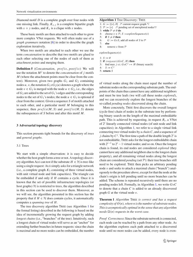
Figure 2 gives a simplified overview of our discovery strat-egy: in a first phase, we seek to discover the highly connectedparts of the physical network (and reserve the correspondingresources, see Lemma 4); this is achieved by trying to embedsequences of so-called “motifs” of the highest connectiv-ity and subsequently shifting toward less connected motifs.Nodes of degree two are found using edge expansion.

4.1 Overview

With the above intuition in mind, we give a short overview ofthis section. In Sect. 4.2, we first formally introduce the con-cept of motifs: simple graphs describing the possible knittingpatterns of a host graph. For example, for a tree graph we

Knitting Expand Links Repeat

Fig. 2 Algorithm Dict first discovers and reserves sequences of highlyconnected parts of the host graph. Then, less connected parts are dis-covered by edge expansion and then the process is repeated until noadditional nodes and edges can be found

only need a single motif, the chain C (two nodes connectedby a link); since there are no 2-connected motifs in a tree, itcan be discovered by attaching chains C to each other.

Another interesting graph family are cactus graphs: con-nected graphs in which any two simple cycles have at mostone vertex in common. Cactus graphs are interesting in thesense that many backbone or core networks are reminiscentof cacti (see, e.g., the topologies collected in the Rocketfuelproject [28]). In terms of motifs, since a cactus graph maycontain cycles, besides the chain C we also need a cycle motifY : three nodes connected in a triangle manner; however, Cand Y are also sufficient to discover all cactus graphs.

More complicated graphs which include higher connectedparts may require, e.g., motifs describing diamonds D orcliques K4. We describe how to extract motifs for a givengraph family in Lemma 3.

The first idea behind our algorithm Dict is that once amotif is embedded, it occupies resources on the entire hostsubgraph (Lemma 4 and Corollary 2), and the discovery of theremaining parts of the subgraph where the motif is embeddedcan be postponed to some later point: For example, Fig. 2(left) shows a motif occupying resources on the subgraph atthe top; additional nodes (Fig. 2 (middle)) and edges (Fig. 2(right)) can be discovered later.

However, in order to discover entire graphs, multiplemotifs are needed: motifs must be attached to each other;accordingly, we introduce the concept of motif sequencesand attachment points (Definition 8). Moreover, for Dict tobe correct, it is important that more highly connected motifsare embedded first: a less connected motif may be embed-dable on a subgraph but may “overlook” (i.e., not allocateresources on) some links. The situation is complicated bythe fact that a graph A may not be embeddable on graph Band vice versa, but A may be embeddable on two graphs B

123


which are attached to each other (see Fig. 3). This motivatesthe dictionary concept (Sect. 4.3) where motifs are organizedin an acyclic directed graph.

Our main result is an algorithm that correctly discovers agiven topology by respect the order of the dictionary of thecorresponding graph family (Theorem 3).

We will give a concrete examples for our concepts and ourapproach throughout this section and describe the explicitrequests issued by our algorithm for a given network inSect. 4.6.

4.2 Motifs: composition and expansion

We now start to make the intuition provided above moreformal.

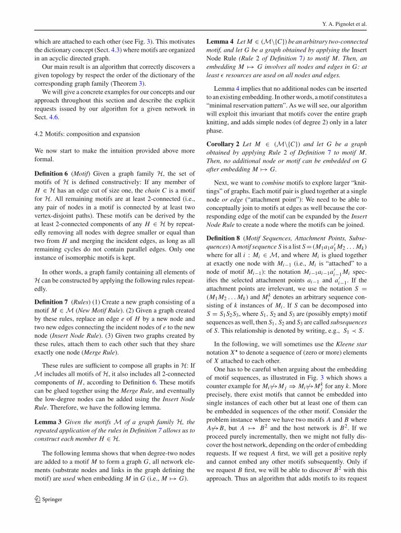
Definition 6 (Motif) Given a graph family H, the set ofmotifs of H is defined constructively: If any member ofH ∈ H has an edge cut of size one, the chain C is a motiffor H. All remaining motifs are at least 2-connected (i.e.,any pair of nodes in a motif is connected by at least twovertex-disjoint paths). These motifs can be derived by theat least 2-connected components of any H ∈ H by repeat-edly removing all nodes with degree smaller or equal thantwo from H and merging the incident edges, as long as allremaining cycles do not contain parallel edges. Only oneinstance of isomorphic motifs is kept.

In other words, a graph family containing all elements ofH can be constructed by applying the following rules repeat-edly.

Definition 7 (Rules) (1) Create a new graph consisting of amotif M ∈ M (New Motif Rule). (2) Given a graph createdby these rules, replace an edge e of H by a new node andtwo new edges connecting the incident nodes of e to the newnode (Insert Node Rule). (3) Given two graphs created bythese rules, attach them to each other such that they shareexactly one node (Merge Rule).

These rules are sufficient to compose all graphs in H: IfM includes all motifs of H, it also includes all 2-connectedcomponents of H , according to Definition 6. These motifscan be glued together using the Merge Rule, and eventuallythe low-degree nodes can be added using the Insert NodeRule. Therefore, we have the following lemma.

Lemma 3 Given the motifs M of a graph family H, therepeated application of the rules in Definition 7 allows us toconstruct each member H ∈ H.

The following lemma shows that when degree-two nodesare added to a motif M to form a graph G, all network ele-ments (substrate nodes and links in the graph defining themotif) are used when embedding M in G (i.e., M �→ G).

Lemma 4 Let M ∈ (M\{C})be an arbitrary two-connectedmotif, and let G be a graph obtained by applying the InsertNode Rule (Rule 2 of Definition 7) to motif M. Then, anembedding M �→ G involves all nodes and edges in G: atleast ε resources are used on all nodes and edges.

Lemma 4 implies that no additional nodes can be insertedto an existing embedding. In other words, a motif constitutes a“minimal reservation pattern”. As we will see, our algorithmwill exploit this invariant that motifs cover the entire graphknitting, and adds simple nodes (of degree 2) only in a laterphase.

Corollary 2 Let M ∈ (M\{C}) and let G be a graphobtained by applying Rule 2 of Definition 7 to motif M.Then, no additional node or motif can be embedded on Gafter embedding M �→ G.

Next, we want to combine motifs to explore larger “knit-tings” of graphs. Each motif pair is glued together at a singlenode or edge (“attachment point”): We need to be able toconceptually join to motifs at edges as well because the cor-responding edge of the motif can be expanded by the InsertNode Rule to create a node where the motifs can be joined.

Definition 8 (Motif Sequences, Attachment Points, Subse-quences) A motif sequence S is a list S =(M1a1a′

1 M2 . . . Mk)

where for all i : Mi ∈ M, and where Mi is glued togetherat exactly one node with Mi−1 (i.e., Mi is “attached” to anode of motif Mi−1): the notation Mi−1ai−1a′

i−1 Mi spec-ifies the selected attachment points ai−1 and a′

i−1. If theattachment points are irrelevant, we use the notation S =(M1 M2 . . . Mk) and Mk

i denotes an arbitrary sequence con-sisting of k instances of Mi . If S can be decomposed intoS = S1S2S3, where S1, S2 and S3 are (possibly empty) motifsequences as well, then S1, S2 and S3 are called subsequencesof S. This relationship is denoted by writing, e.g., S1 ≺ S.

In the following, we will sometimes use the Kleene starnotation X� to denote a sequence of (zero or more) elementsof X attached to each other.

One has to be careful when arguing about the embeddingof motif sequences, as illustrated in Fig. 3 which shows acounter example for Mi �→M j ⇒ Mi �→Mk

j for any k. Moreprecisely, there exist motifs that cannot be embedded intosingle instances of each other but at least one of them canbe embedded in sequences of the other motif. Consider theproblem instance where we have two motifs A and B whereA �→B, but A �→ B2 and the host network is B2. If weproceed purely incrementally, then we might not fully dis-cover the host network, depending on the order of embeddingrequests. If we request A first, we will get a positive replyand cannot embed any other motifs subsequently. Only ifwe request B first, we will be able to discover B2 with thisapproach. Thus an algorithm that adds motifs to its request

123


Fig. 3 Left: Motif A. Center: Motif B. Observe that A �→B. Right:Motif A is embedded into two consecutive Motifs B: solid lines arevirtual links mapped on single substrate links, solid curves are virtuallinks mapped on multiple substrate links, dotted lines are substrate links

implementing a multi-hop virtual link, and dashed lines are substrateunused links. Grayed nodes are relay-only nodes. Observe that the cen-tral node has a relaying load of 4ε

networks purely incrementally in an arbitrary order cannotdiscover all substructures. This is the motivation for intro-ducing the concept of a dictionary which imposes an orderon motif sequences and their attachment points.

4.3 Dictionary structure and existence

In a nutshell, a dictionary is a Directed Acyclic Graph(DAG) defined over all possible motifs M and imposes anorder (poset relationship �→) on problematic motif sequenceswhich need to be embedded one before the other (e.g., thecomposition depicted in Fig. 3). To distinguish them fromsequences, dictionary entries are called words.

Definition 9 (Dictionary, Words) A dictionary D(VD, ED)

is a Directed Acyclic Graph (DAG) over a set of motifsequences VD together with their attachment points. In thecontext of the dictionary, we will call a motif sequence word.The links ED represent the poset embedding relationship �→.

Concretely, the DAG has a single root r , namely the chaingraph C (with two attachment points). In general, the attach-ment points of each vertex v ∈ VD describing a word w,define how w can be connected to other words. The directededges ED = (v1, v2) represent the transitively reducedembedding poset relation with the chain C context: Cv1C isembeddable in Cv2C and there is no other word Cv3C suchthat Cv1C �→ Cv3C , Cv3C �→ Cv2C and Cv3C �→Cv1Cholds. (The chains before and after the words are added toensure that attachment points are “used”: there is no edgebetween two isomorphic words with different attachmentpoint pairs.)

We require that the dictionary be robust to composition:For any node v, let Rv = {v′ ∈ VD, v �→ v′} denote the“reachable” set of words in the graph and Rv = VD\Ri allother words. We require that v �→W for all W ∈ Qi :=R

�

i \R�i , where the transitive closure operator X� denotes an

arbitrary sequence (including the empty sequence) of ele-ments in X (according to their attachment points).

See Fig. 4 for an example. Informally, the robustnessrequirement means that the word represented by v can-

(a)

D

Dc

b

D

d

a

B

d e

B

e

B

C Y

K

K

e

K

d

K

e

K

ed

d

1 2

1

3

1

1

1

1

2

1

1

4

2

3d

a

c

b

d

d e

ed

d

e

db

c

a

(b)

Fig. 4 a Example dictionary with motifs Chain C , Cycle Y , DiamondD, complete bipartite graph B = K2,3 and complete graph K = K5.The attachment point pair of each word is black, the other nodes andedges of the words are grey. The edges of the dictionary are locallylabeled, which is used in Dict later. b A graph that can be constructedfrom the dictionary words

not be embedded in any sequence of “smaller” words, unlessa subsequence of this sequence is in the dictionary as well.As an example, consider a dictionary containing the motifsA and B from Fig. 3: this dictionary would not only containvertices A and B but also B B, as well as a path from A toB B. In the following, we use the notation maxv∈VD (v �→ S)

to denote the set of “maximal” vertices with respect to theirembeddability into S : i ∈ maxv∈VD (v �→ S) ⇔ (i �→S) ∧ (∀ j ∈ �+(i), j �→S), where �+(v) denotes the set of

123


outgoing neighbors of v. Furthermore, we say that a dic-tionary D covers a motif sequence S iff S can be formedby concatenating dictionary words (henceforth denoted byS ∈ D�) at the specified attachment points. More generally,a dictionary covers a graph, if it can be formed by mergingsequences of D�.

Let us now derive some properties of the dictionary whichare crucial for a proper substrate topology discovery. Firstwe consider maximal dictionary words which can serve asembedding “anchors” in our algorithm.

Lemma 5 Let D be a dictionary covering a sequence S ofmotifs, and let i ∈ maxv∈VD (v �→ S). Then i constitutes asubsequence of S, i.e., S can be decomposed to S1i S2, and Scontains no words of order at most i , i.e., S1, S2 ∈ (Ri ∪{i})�.

The following corollary is a direct consequence of the def-inition of i ∈ maxv∈VD (v �→ S) and Lemma 5: for a motifsequence S with S ∈ (Ri ∪ {i})�, all the subsequences of Sthat contain no i are in R

�

i . As we will see, the corollary is use-ful to identify the motif words composing a graph sequence,from the most complex words to the least complex ones.

Corollary 3 Let D be a dictionary covering a motif sequenceS, and let i ∈ maxv∈VD (v �→ S). Then S can be decomposedas a sequence S = T1iT2i, . . . , iTk with Tj ∈ Qi for allj = 1, . . . , k.

This corollary can be applied recursively to describe amotif sequence as a sequence of dictionary entries. Note thata dictionary always exists.

Lemma 6 There exists a dictionary D = (VD, ED) thatcovers all member graphs H of a motif graph family H withn vertices.

Note that the proof of Lemma 6 only addresses the compo-sition robustness for sequences of up to n nodes. However,it is clear that |V (G)| > |V (H)| ⇒ G �→H . Therefore itcannot happen that a request of a sequence with more than nnodes is answered positively on a host network of n nodes andhence this limitation does not pose an issue when devisingdictionary-based algorithms for VNet topology discovery.

4.4 The dictionary algorithm

With these concepts in mind, we are ready to present Dictin detail (cf Algorithm 2). Basically, Dict always grows arequest graph G = H ′ until it is isomorphic to H (the graphto be discovered). This graph growing is performed accordingto the dictionary, i.e., we try to embed new motifs in the orderimposed by the dictionary DAG.

Algorithm 2 Motif Graph Discovery Dict1: H ′ := {{v},∅} /*current request graph*/,

P := {v} /*set of unexplored nodes*/2: while P = ∅ do3: choose v ∈ P , T := findMotifSequence(v,∅,∅)

4: if (T = ∅) then H ′ := H ′vT , add all nodes of T to P , for alle ∈ T do edgeExpansion(e)

5: else remove v from PfindMotifSequence(v, T<, T>)1: find maximal i, j, Bf, Af s.t. H ′v (T<) Bf (D[i]) j Af (T>) �→ H

where Bf, Af ∈ {∅, C}2 /* issue requests */2: if ((i, j, Bf, Af) = (0, 0, C,∅)) then return T<CT>

3: if (Bf = C) then Bf = findMotifSequence(v, T<, (D[i]) j Af T>)

4: if (Af = C) then Af = findMotifSequence(v, T< Bf (D[i]) j , T>)

5: return Bf (D[i]) j Af

edgeExpansion(e)1: let u, v be the endpoints of edge e, remove e from H ′2: find maximal j s.t. H ′vC j u �→ H /* issue requests */3: H ′ := H ′vC j u, add newly discovered nodes to P

Let us specify the topological order in which algo-rithm Dict discovers the dictionary words. First, for eachnode v in VD , we define an order on its outgoing edges{(v,w)|w ∈ �+(v)}. This order is sometimes referred to asa port labeling, and each path from the dictionary root (thechain C) to a node in VD can be represented as the sequenceof port labels at each traversed node (l1, l2, . . . , ll), where l1corresponds to a port number in C . We can simply use thelexicographic order on integers, <d : (a1, a2, . . . , an1) <d

(b1, b2, . . . , bn2) ⇐⇒ ((∃ m > 0) (∀ i < m)(ai =bi )∧(am < bm))∨(∀i ∈ {1, . . . n1}, (ai = bi )∧(n1 < n2)),to associate each vertex with its minimal sequence, and sortvertices of VD according to their embedding order. Let r bethe rank function associating each vertex with its position inthis sorting: r : VD → {1, . . . |VD|} (i.e., r is the topologicalordering of D).

The fact that subsequences can be defined recursivelyusing a dictionary (Lemma 5 and Corollary 3) is exploited byalgorithm Dict. Concretely, we apply Corollary 3 to gradu-ally identify the words composing a graph sequence, fromthe most complex words to the least complex ones. Thisis achieved by traversing the dictionary depth-first, startingfrom the root C up to a maximal node: algorithm Dict teststhe nodes of �+(v) in increasing port order as defined above.As a shorthand, the word v ∈ VD with r(v) = i is written asD[i]; similarly D[i] < D[ j] holds if r(D[i]) < r(D[ j]), anotation that is useful since D[ j] is detected before D[i] byalgorithm Dict. As a consequence, the first matched wordof a sequence S is unique: it is i = arg maxx (D[x] �→ S) =max{r(v)|v ∈ maxv′∈VD (v′ �→ S)}, the maximal word in S.

Algorithm Dict distinguishes whether the subsequencesnext to a word v ∈ VD are empty (∅) or chains (C), andwe will refer to the subsequence before v by Bf and to thesubsequence after v by Af. Concretely, while recursively

123


exploring a sequence between two already discovered partsT< and T> we check whether the maximal word v is directlynext to T< (i.e., T< v, . . . , T>) or T> or both (∅), or whether v

is somewhere in the middle. In the latter case, we add a chain(C) to be able to find the greatest possible word in a nextstep.

Dict uses tuples of the form (i, j, Bf, Af) where i, jare integers and (Bf, Af) ∈ {∅, C}2, i.e., D[i] denotesthe maximal word in D, j is the number of consecutiveoccurrences of the corresponding word, and Bf and Af rep-resent the words before and after D[i]. These tuples arelexicographically ordered by the total order relation > onthe set of possible (i, j, Bf, Af) tuples defined as follows:let t = (i, j, Bf, Af) and t ′ = (i ′, j ′, Bf′

, Af′) two such

tuples. Then t > t ′ iff w > w′ or w = w′ ∧ j > j ′ orw = w′ ∧ j = j ′ ∧ Bf = C ∧ Bf′ = ∅ or w = w′ ∧ j =j ′ ∧ Bf = Bf′ ∧ Af = C ∧ Af′ = ∅.

With these definition we can prove that algorithm Dict iscorrect.

Theorem 3 Given a dictionary for H, algorithm Dict cor-rectly discovers any H ∈ H.

4.5 Request complexity

The focus of Dict is on generality rather than performance,and indeed, the resulting request complexities can often behigh. However, as we will see, there are interesting graphclasses which can be solved efficiently.

Let us start with a general complexity analysis. Therequests issued by Dict are constructed in Line 1 off inding_moti f _sequence() and in Line 2 of edgeExpan-sion(). We will show that the request complexity of the lat-ter is linear in the number of edges of the host graph whilethe request complexity of f inding_moti f _sequence()depends on the structure of the dictionary. Essentially, an effi-cient implementation of Line 1 of f inding_moti f _sequencein Dict can be seen as the depth-first exploration of the dic-tionary D starting from the chain C . More precisely, at adictionary word v requests are issued to see if one of the out-going neighbors of v could be embedded at the position of v.As soon as one of the replies is positive, we follow the corre-sponding edge and continue recursively from there, until nooutgoing neighbors can be embedded. Thus, the number ofrequests issued before we reach a vertex v can be determinedeasily.

Recall that Dict tests vertices of a dictionary D accord-ing to a fixed port labeling scheme. For any v ∈ VD ,let p(C, v) be the set of paths from C to v (each pathincluding C and v). In the worst case, discovering v costscost (v) = maxp∈p(C,v)(

∑u∈p |�+(u)|).

Lemma 7 The request complexity of Line 1 of findMotifSequence(v′, T<, T>) to find the maximal i, j, Bf, Af such

D

Y

D

B

D

Y

Y

C

C

C

C

C

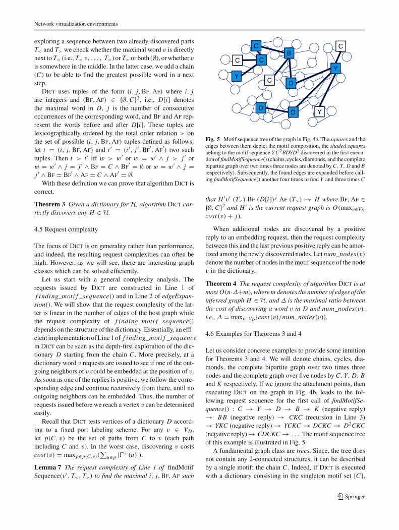
Fig. 5 Motif sequence tree of the graph in Fig. 4b. The squares and theedges between them depict the motif composition, the shaded squaresbelong to the motif sequence Y C2BDYD2 discovered in the first execu-tion of findMotifSequence() (chains, cycles, diamonds, and the completebipartite graph over two times three nodes are denoted by C, Y, D and Brespectively). Subsequently, the found edges are expanded before call-ing findMotifSequence() another four times to find Y and three times C

that H ′v′ (T<) Bf (D[i]) j Af (T>) �→ H where Bf, Af ∈{∅, C}2 and H ′ is the current request graph is O(maxv∈VD

cost (v) + j).

When additional nodes are discovered by a positivereply to an embedding request, then the request complexitybetween this and the last previous positive reply can be amor-tized among the newly discovered nodes. Let num_nodes(v)

denote the number of nodes in the motif sequence of the nodev in the dictionary.

Theorem 4 The request complexity of algorithm Dict is atmost O(n·Δ+m), where m denotes the number of edges of theinferred graph H ∈ H, and Δ is the maximal ratio betweenthe cost of discovering a word v in D and num_nodes(v),i.e., Δ = maxv∈VD {cost (v)/num_nodes(v)}.

4.6 Examples for Theorems 3 and 4

Let us consider concrete examples to provide some intuitionfor Theorems 3 and 4. We will denote chains, cycles, dia-monds, the complete bipartite graph over two times threenodes and the complete graph over five nodes by C, Y, D, Band K respectively. If we ignore the attachment points, thenexecuting Dict on the graph in Fig. 4b, leads to the fol-lowing request sequence for the first call of findMotifSe-quence() : C → Y → D → B → K (negative reply)→ B B (negative reply) → CKC (recursion in Line 3)→ YKC (negative reply) → YCKC → DCKC → D2CKC(negative reply) → CDCKC → . . .. The motif sequence treeof this example is illustrated in Fig. 5.

A fundamental graph class are trees. Since, the tree doesnot contain any 2-connected structures, it can be describedby a single motif: the chain C . Indeed, if Dict is executedwith a dictionary consisting in the singleton motif set {C},

123


it is equivalent to a recursive version of Tree from [21] andseeks to compute maximal paths.

Corollary 4 Trees can be described by one motif (the chainC) .The request complexity of Dict on trees is O(n).

Proof Since there is only one motif and it has only oneattachment point pair, Δ of the dictionary is constant. Con-sequently, a linear request complexity follows directly fromTheorem 4 due to the planarity of cactus graphs (i.e., m ∈O(n)). ��An example where the dictionary is efficient although theconnectivity of the topology can be high, are block graphs.A block graph is an undirected graph in which every bi-connected component (a block) is a clique. A generalizedblock graph is a block graph where the edges of the cliquescan contain additional nodes. In other words, in the terminol-ogy of our framework, the motifs of generalized block graphsare cliques. For instance, cactus graphs are generalized blockgraphs where the maximal clique size is three.

Corollary 5 Generalized block graphs can be described bythe motif set of cliques. The request complexity of Dict ongeneralized block graphs is O(m), where m denotes the num-ber of edges in the host graph.

Proof The framework dictionary for generalized blockgraphs consists of the set of cliques, as a clique with k nodescannot be embedded on sequences of cliques with less thank nodes. As there are three attachment point pairs for eachcomplete graph with four or more nodes, Dict can be appliedusing a dictionary that contains three entries for each motifwith more than three nodes (num_nodes() > 3). Thus, thei th dictionary entry has �i/3� + 3 nodes for i > 1 andcost (D[i]) < 3(i + 2) and Δ of D is hence in O(1). Conse-quently the complexity for generalized block graphs is O(m)

due to Theorem 4. ��On the other hand, Theorem 4 also states that highly con-

nected graphs may require �(n2) requests, even if the dic-tionary is small.

4.7 Extended example: cactus graphs

We conclude the discussion of the framework with anextended example for cactus graphs. As already mentioned,cactus graphs are a particularly interesting topology in thecontext of the Internet. For example, the topologies collectedin experiments such as Rocketfuel are often sparse but con-tain certain cycles along the backbone, and thus resemble thecactus graph [28]. Formally, a cactus graph is a connectedgraph in which any two simple cycles have at most one ver-tex in common. Or equivalently: every edge in the cactusgraph belongs to at most one 2-connected component, i.e.,

the cactus graph does not contain any diamond graph shapedminors.

The motif set for cactus contains only cycles (short form:Y ) and chains (short form: C). Since cycles are symmetric,the dictionary required to discover cactus graphs is very sim-ple: {C, Y }. Due to this simplicity it is possible to unfold therecursions in Dict to produce a iterative and compact algo-rithm to discover cactus topologies: the algorithm Cactus.This might prove useful for implementations and provides adifferent perspective to the reader. Note that in contrast to atree where nodes are origins of simple paths (i.e., branches),a cactus graphs is very simple: C, Y . Due to this simplicityit is possible to unfold the recursions in Dict to produce astandalone iterative and compact algorithm to discover cactustopologies: the Cactus algorithm. Note that in contrast to atree where nodes are origins of simple paths (i.e., branches),a cactus node can be the origin of several sub-cactus graphsconsisting of 1- and 2-connected components. That is, theresulting graph when collapsing one or several 2-connectedcomponents to a single node is a cactus as well, or even a treeif all components are collapsed. The structure of Cactusis therefore similar to Tree in its iterative approach. Con-cretely, instead of using longest chains as “anchor points”for extending an existing topology, we search, in each pos-sible direction from a pending cactus node v for a maximalsequences of cycles and chains. Only once such a sequence(or “motif ”) is found, our algorithm Cactus finds out thedetailed structure of the chain/cycle sequence by inserting asmany nodes on the chains and cycles as possible.

The formal listing of Cactus appears in Algorithm 3.Since the algorithm is no longer recursive as the Dict algo-rithm and only requires two motifs, we can prove its correct-ness and request complexity more easily.

Theorem 5 Cactus discovers any cactus topology withrequest complexity O(n). This is asymptotically optimal.

Proof Correctness: Since by definition, the cactus graphdoes not contain any diamond graph shaped minor graphs,no two finite faces of the cactus graph can share a link (butsharing nodes is possible), and hence, any node v connects aset of (sub)cactus graphs.

Starting with one node, Cactus repeatedly finds asequence S of cycles (Y ) and chains (C) with exploreSe-quence() and then expands these cycles and chains to find allnodes lying on them with edgeExpansion(). This algorithmterminates as soon as all edges incident to nodes found so far(i.e., pending nodes) have been discovered. Consequently, weneed to show that all nodes and all their adjacent edges aredetected in order to prove correctness (i.e., there is a bijectionbetween the edges in G and in H and thus it is not possiblethat a virtual edge connects two nodes that are not adjacentin the (sub)cactus graphs).

123


Algorithm 3 Cactus Discovery: Cactus1: G := {{v},∅} /* current request graph */2: P := {v} /* pending set of unexplored nodes*/3: while P = ∅ do4: choose v ∈ P , S :=exploreSequence(v)5: if S = ∅ then6: G := GvS, add all nodes of S to P7: for all e ∈ S do edgeExpansion(e)8: else9: remove v from P

exploreSequence(v)1: S := ∅, P ′′ := ∅2: if GvY CY �→ H then3: find max j s.t. GvY j CY �→ H4: S := Y j CY , P ′ := {C}5: while P ′ = ∅ do6: for all Ci ∈ P ′ do7: A := pre f i x(Ci , S), B := post f i x(Ci , S);8: if GvACY C B �→ H then9: find max j, k s.t. GvAC(Y j C)k B �→ H10: for l := 1, . . . , k do11: P ′′ := P ′′ ∪ {Cl }12: S := AC(Y j C)k B13: P ′ := P ′′, P ′′ := ∅14: if request(GvSY, H) then15: find max j s.t. GvSY j �→ H16: S := SY j

17: if request(GvSC, H) then18: S := SC19: return S

edgeExpansion(e)1: let u, v be the endpoints of edge e, remove e from G2: find max j s.t. GvC j u �→ H3: G := GvC j u, add newly discovered nodes to P

Note that the algorithm maintains the invariant thatGvS �→ H at all times. As a consequence we can analyzethe properties of S and thereby deduce properties of the sub-strate. We start by proving that for a sequence S discoveredin exploreSequence(v) the following properties hold: (i) nomore Y s can be inserted (replace a Y by a YY or a C bya CYC), (i i) no chain can be inserted between two cycles(replace YY with YCY) and (i i i) no C can be replaced by a Y .These invariants show that the discovered sequence S can-not be extended with more cycles or chains between cycles.Based on these invariants it remains to show that in the fol-lowing steps of the algorithm we discover all nodes whichare part of this sequence.

(i) If there are cycles attached to v directly, their maximalundetected concatenated occurrence is discovered in Line 3(i.e., if GvY j �→ H, j maximum, it is not possible that theremaining topology of H after the embedding π(G) con-tains a sequence starting at v with more than j concatenatedcycles). Within one execution of the forall loop (Line 6-13)the maximal value j reaches, decreases in the next executionof the loop. For each chain Ci treated in the forall loop it

holds that all Y j occurrences are discovered (guaranteed byLine 9) and thus it is not possible to replace any Y by YY.Replacing a C by a CYC is not possible since this is checkedfor all C in Line 9 of exploreSequence(v). The last C thatmight be appended to S in Line 19 cannot be replaced byCYC as this would have happened in Line 9. (i i) ReplacingS = AYYB by AYCYB is only possible if the substrate con-tains AYYYB and B starts with C , i.e., it would invalidate (i)and is thus impossible. (i i i) Every C of S is between two Y .If C could be replaced by a Y this would have been discov-ered in Line 3 or 9 and is thus not possible anymore at theend of exploreSequence(v).

As a consequence of Properties (i), (i i), (i i i) it holds thatwith S all nodes of degree one or nodes that lie at the intersec-tion of cycles and chains or cycles and cycles (i.e., nodes withdegree three or four in S) are detected in exploreSequence(v).For a given sequence S the remaining nodes of degree twoin S are discovered in edgeExpansion(e). It thus remainsto prove that among these discovered nodes the ones withhigher degrees are further explored for additional sequencesattached to them. As all nodes are added to P when they arediscovered (Line 6 of Algorithm 3, and Line 3 of the subrou-tine edgeExpansion(e)), and as the while loop in Line 3 isrepeated until there are no outgoing sequences from a nodeanymore, all cactus edges are detected. Any additional edgewould lead to a diamond minor, resulting in a contradiction.

Complexity: We can again use an amortization schemethat assigns request costs to edges: an edge is assigned thecost of the request where it is identified for the first time (inexploreSequence(v) this can happen at Lines 2, 3, 8, 9, 15,16, 18, in edgeExpansion(e) in Line 2). In order to find themaximum embeddable sequence, there is one request with anegative answer in the execution of Lines 3, 9, 16 in explore-Sequence(v) and Line 2 in edgeExpansion(e). Let us assignthese unsuccessful requests that do not discover a new edgeto the last edge discovered before. Thus in the worst case,there are two requests for each edge. Since the number ofedges in cactus graphs is linear in the number of nodes, arequest complexity of O(n) follows.

Optimality: Since cactus graphs constitute a super-set oftree graphs, the lower bound of Theorem 1 still applies, i.e.,�(n) requests are needed by any algorithm. ��

5 Simulations

To complement our theoretical results and to validate ourframework on real network topologies, we dissected the ISPtopologies provided by the Rocketfuel [28] mapping engine.In particular, given the high execution times of Dict in theworst-case and for complex motif sets, we were interestedin (1) the structure and complexity of the motif sets of thesetopologies, and in (2) the question whether an efficient and

123


(a)

0

2500

5000

7500

1221

1239

1755

2914

3257

3356

3967

4755

7018

Topology

Nu

mb

er o

f n

od

es orig

inal

tree

edge

Exp

bigg

est

(b)

(c)

0.00

0.25

0.50

0.75

1.00

1221

1239

1755

2914

3257

3356

3967

4755

7018

Topology

Rat

io o

f n

od

es d

isco

vere

d (d)

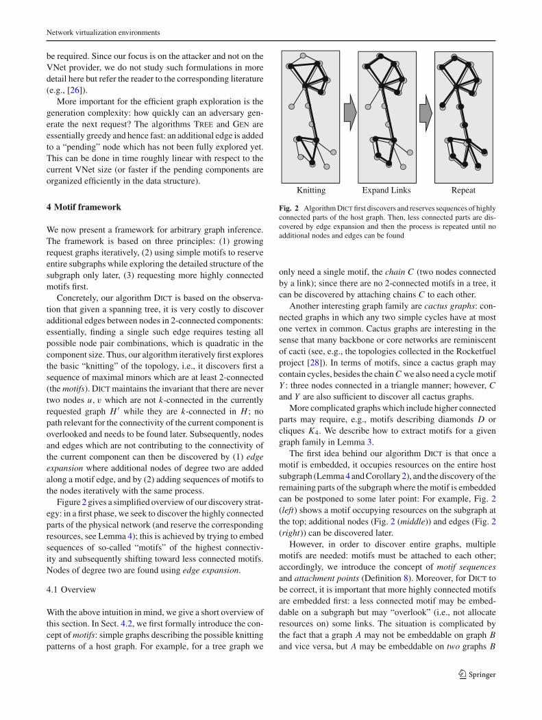
Fig. 6 Results of Dict when run on different Internet and power gridtopologies. a Number of nodes in different autonomous systems (AS).We computed the set of motifs of these graphs as described in Defini-tion 6 and counted the number of remaining nodes after removing thenodes that : (i) belong to a tree structure at the “fringe” of the network,

(ii) have degree 2 and belong to two-connected motifs, and finally (iii)are part of the largest motif. b The 19-motif dictionary built from thedataset. c The fraction of nodes that can be discovered with the dictio-nary. d Most frequent motifs encountered in the dataset

approximate variant of Dict could be used in practice to inferlarge parts of the network in linear time.

For this purpose, we implemented our motif extractionalgorithm. Concretely, for each Rocketfuel topology, we firstisolate the subgraphs that are trees (i.e., the 1-connected sub-graphs), by recursively removing leaf-nodes. The remainderof the topology is then simplified by contracting degree-2nodes that would be detected during the algorithms’ edgeexpansion phases. The result is a topology only containingmotifs connected by “articulation vertices”, which provideus with a mean to distinguish motifs. Finally, the extractedmotifs are compared pairwise to distinguish between iso-morphic and non-isomorphic ones. (The corresponding Rscript is made publicly available at http://homepages.laas.fr/~gtredan/topoInference.R.)

Figure 6a provides some statistics about the consideredAS router-level topologies: their overall size, the numberof nodes belonging to a 1-connected subgraph, the num-ber of nodes belonging to a motif, and the number of nodesbelonging to the largest motif of each topology. For instance,the figure shows that the AS 1221 topology contains 2669nodes, but only 310 nodes are part of a bi-connected compo-nent. Among those nodes, 47 are expanded degree-2 nodes,

and 48 are part of motifs containing only 3 or 4 nodes. Theremaining 215 nodes compose the “network heart” (contain-ing 716 edges out of the topologies’ 3175 edges): such a sin-gle highly-connected motif is typical and appears for manyAS topologies. One takeaway from this plot is that, sincemost Rocketfuel networks are built of simple motifs and sinceDict discovers both tree and relay nodes easily, most of eachtopology could be discovered quickly with an approximateDict algorithm containing merely the basic motifs: only thefew more complex motifs in the network heart require anexhaustive link exploration. In other words, the vast majorityof the topology can be discovered in linear time.

Figure 6b, c further explore the fraction of nodes that canbe discovered by Dict restricted to a small motif set. For thispurpose, we built a dictionary containing all the motifs iden-tified in our dataset, and removed the biggest motif of eachtopology (the “network heart”). The remaining 19 motifs aredepicted Fig. 6b: they are surprisingly simple and symmetric.Figure 6c shows the fraction of nodes in perfectly inferredsubgraphs: we see that a 19-motifs dictionary is sufficient toexplore from 37 to 92 % of the nine considered AS topologies.Figure 6d represents the frequency distribution of the mostcommon motifs in the nine topologies. Note that interest-

123

http://homepages.laas.fr/~gtredan/topoInference.R

http://homepages.laas.fr/~gtredan/topoInference.R


Fig. 7 Representation of the AS-4755 network where tree nodes arecolored yellow, relay-nodes are green, attachment point nodes are red,cYcle motifs nodes are purple and the maximal motif nodes are blue(color figure online)

ingly, motif Y only comes third, with 11 occurrences acrossthe dataset.

To conclude our study of ISP network motifs, in Fig. 7we show an example for how the motifs cover a specific AStopology (namely AS-4755).

6 Related work

Our work is motivated by the virtualization trend in today’sInternet and especially network virtualization. For a generalintroduction and a good survey, we refer the reader to [8].Our model differentiates between a customer (e.g., a ser-vice provider requesting VNets) and a substrate provider(e.g., a physical infrastructure provider or a virtual networkprovider). In the terminology of [27], our customer is the SP,and the provider may either be the PIP or the VNP.VNet embedding The embeddings of VNets is an intensivelystudied problem and there exists a large body of literature(e.g., [13,14,18,31]), and there also exist distributed com-puting approaches [16] and online algorithms [5,11]. Ourwork is orthogonal to this line of literature in the sense thatwe assume that an (arbitrary and not necessarily resource-optimal) embedding algorithm is given. Rather, we focuson the question of how the feedback obtained through thesealgorithms can be exploited, and we study the implicationson the information which can be obtained about a provider’sinfrastructure.Topology inference Our work studies a new kind of topol-ogy inference problems. Traditionally, much graph discoveryresearch has been conducted in the context of today’s com-plex networks such as the Internet which have fascinated

scientists for many years, and there exists a wealth of resultson the topic. One of the most influential measurement stud-ies on the Internet topology was conducted by the Faloutsosbrothers [12], and their work has subsequently been inten-sively discussed both in practical [17] and theoretical [2]papers. The classic instrument to discover Internet topolo-gies is traceroute [7], but the tool has several problems whichrenders the problem challenging. One complication of tracer-oute stems from the fact that routers may appear as stars(i.e., anonymous nodes), which renders the accurate charac-terization of Internet topologies difficult [1,23,30]. Networktomography is another important field of topology discovery.In network tomography, topologies are explored using pair-wise end-to-end measurements, without the cooperation ofnodes along these paths. This approach is quite flexible andapplicable in various contexts, e.g., in social networks. For agood discussion of this approach as well as results for a rout-ing model along shortest and second shortest paths see [4].For example, [4] shows that for sparse random graphs, a rel-atively small number of cooperating participants is sufficientto discover a network fairly well.

Both the traceroute and the network tomography problemsdiffer from our virtual network topology discovery problemin that the exploration there is inherently path-based whilewe can ask for entire virtual graphs.Virtualization and security The benefits and threats of virtu-alization are extensively studied but still not well-understood.A complete review of the research is beyond the scope of thispaper, and we refer the reader to the recent literature, e.g., onvirtual machine collocation attacks [25].Graph grammars and mining We decided to describe ouralgorithms using a graph grammar formalism, and indeed,some graph grammar problems share commonalities with ourwork. Graph grammars are a powerful tool to generate andcharacterize topologies, and we refer the interested reader to,e.g., [6]. More remotely, our work also has connections withgraph data mining [29]. For instance, in [9], an algorithmis presented to search subsequences which can best com-press an input graph based on a minimum description lengthprinciple. Although these algorithms pursue a different goal,the computationally-constrained beam search is reminiscentof some of our techniques as nodes are incrementally (andgreedily) expanded.Bibliographic note Our article builds upon our model intro-duced in a Brief Announcement at DISC [20]; the tree andcactus related results appeared at INFOCOM 2013 [21] andthe dictionary was presented at NETYS 2013 [22].

7 Conclusion

This paper has initiated, from an algorithmic perspective, thediscussion of topology discovery in network virtualization

123


environments, and presented tight bounds for three importantgraph classes. We understand our results as a first step toshed light on possible security threats of the virtualizationtechnology.

We find that the topology of typical sparse backbone net-works such as tree or cactus graphs can be discovered rela-tively fast (request complexity O(n)). However, the motif-based topology discovery framework we sketched suggeststhat the request complexity for denser graphs is higher, as thenumber of graph knittings can grow combinatorially, and onehas to resort to testing edges individually (after computing aspanning tree) which yields a quadratic request complexity.

Our work opens several interesting directions for futureresearch. First, more work is needed to understand the impli-cations of the framework on other important graph classes,such as different types of planar graphs: in order to beat thetrivial O(n2) upper bound on the request complexity, addi-tional dictionary properties must be exploited.

Moreover, in the context of Tree we have seen that if thehost graph is not a tree, running Tree will simply result in aspanning tree. This raises the question whether similar span-ning structures can be computed with incomplete motif sets,resulting in the “densest spanning structures” given thesemotif sets. For example, when applying Cactus to a generalgraph, which fraction of edges will be discovered?

Finally, while our work so far has focused on discoveringthe entire topology, more specific graph properties may beinferred much more efficiently.

Acknowledgments We would like to thank Georgios Smaragdakisfrom Telekom Innovation Laboratories for interesting discussions.Part of this work was performed within the Virtu project, funded byNTT DOCOMO Euro-Labs, and the Collaborative Networking project,funded by Deutsche Telekom AG. We would like to thank all our col-leagues in these projects

Appendix 1: Proof of Lemma 1

We prove the lemma for undirected graphs. The extension todirected graphs is straight-forward.

A poset structure (S,�) over a set S requires that � isa (reflexive, transitive, and antisymmetric) order which mayor may not be partial. To show that (G, �→), the embeddingorder defined over a given set of graphs G, is a poset, weexamine the three properties in turn.

Reflexivity (for each G ∈ G, G �→ G): By using theidentity mapping π : G = (V, E) → G = (V, E) whichembeds each node and link to itself, the claim is proved.

Transitivity (for all A, B, C ∈ G, if A �→ B and B �→ Cthen A �→ C): Let π1 denote the embedding function forA �→ B and let π2 denote the embedding function for B �→C , which must exist by our assumptions. We will show thatthen also a valid embedding function π exists to map A to

C . Regarding the node mapping, we define πV as πV :=π1V ◦π2V , i.e., the result of first mapping the nodes accordingto π1V and subsequently according to π2V . We first show thatπV is a valid mapping from A to C as well. First, for all vA ∈VA, π(vA) maps vA to a single node in VC , fulfilling the firstcondition of the embedding (see Definition 1). Ignoring relaycapacities (which is studied together with the conditions onthe links below), Condition (i i) of Definition 1 is also fulfilledsince the mapping π1V ensures that no node in VB exceeds itscapacity, and can hence safely be mapped to VC . Let us nowturn our attention to the links. We use the following mappingπE for the edges. Note that π1E maps a single link e to anentire (but possibly empty) path in B and π2E then maps thecorresponding links e′ in B to a walk in C . We can transformany of these walks into paths by removing cycles; this canonly lower the resource costs. Since π1E maps to a subset ofEB only and since π2E can embed all edges of B, all linkcapacities are respected up to relay costs. However, note alsothat by the mapping π1 and for relay costs ε > 0, each nodevB ∈ VB can either not be used at all, be fully used as asingle endpoint of a link eA ∈ E A, or serve as a relay forone or more links. Since both end-nodes and relay nodes aremapped to separate nodes in C , capacities are respected aswell. Conditions (i i i) and (iv) hold as well.

Antisymmetry (for all A, B ∈ G, A �→ B and B �→ Aimplies A = B, i.e., A and B are isomorphic): First observethat if the two networks differ in size, i.e., |VA| = |VB | or|E A| = |EB |, then they cannot be embedded to each other:Without loss of generality, assume |VA| > |VB |, then sincenodes of VA of cannot be split into multiple nodes of VB

(cf Definition 1), there exists a node vA ∈ VA to which nonode from VB is mapped. This however implies that nodeπ1(vA) ∈ VB must have available capacities to host also vA,contradicting our assumption that nodes cannot be split in theembedding. Similarly, if |E A| = |EB |, we can obtain a con-tradiction with the single path argument. Thus, not only thetotal number of nodes and links in A and B must be equivalentbut also the total amount of node and link resources. So con-sider a valid embeddingπ1 for A �→ B and a valid embeddingπ2 for B �→ A, and assume |VA| = |VB | and |E A| = |EB |.It holds that π1 and π2 define an isomorphism between Aand B: Clearly, since |VA| = |VB |, π1 and π2 define a per-mutation on the vertices. Without loss of generality, considerany link {vA, v′

A} ∈ E A. Then, also {π1(vA), π1(v′A)} ∈ EB :

|{π1(vA), π1(v′1)}| = 0 would violate the node capacity con-

straints in B, and |{π1(vA), π1(v′A)}| > 1 requires |EB | >

|E A|.


(i) From Definition 1, A �→ B defines a mapping π from VA

to VB and from E A to EB , which implies that the subgraph

123


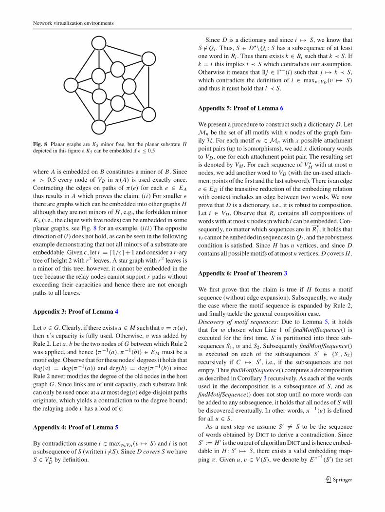
Fig. 8 Planar graphs are K5 minor free, but the planar substrate Hdepicted in this figure a K5 can be embedded if ε ≤ 0.5

where A is embedded on B constitutes a minor of B. Sinceε > 0.5 every node of VB in π(A) is used exactly once.Contracting the edges on paths of π(e) for each e ∈ E A

thus results in A which proves the claim. (i i) For smaller ε

there are graphs which can be embedded into other graphs Halthough they are not minors of H , e.g., the forbidden minorK5 (i.e., the clique with five nodes) can be embedded in someplanar graphs, see Fig. 8 for an example. (i i i) The oppositedirection of (i) does not hold, as can be seen in the followingexample demonstrating that not all minors of a substrate areembeddable. Given ε, let r = �1/ε�+1 and consider a r -arytree of height 2 with r2 leaves. A star graph with r2 leaves isa minor of this tree, however, it cannot be embedded in thetree because the relay nodes cannot support r paths withoutexceeding their capacities and hence there are not enoughpaths to all leaves.


Let v ∈ G. Clearly, if there exists u ∈ M such that v = π(u),then v’s capacity is fully used. Otherwise, v was added byRule 2. Let a, b be the two nodes of G between which Rule 2was applied, and hence {π−1(a), π−1(b)} ∈ EM must be amotif edge. Observe that for these nodes’ degrees it holds thatdeg(a) = deg(π−1(a)) and deg(b) = deg(π−1(b)) sinceRule 2 never modifies the degree of the old nodes in the hostgraph G. Since links are of unit capacity, each substrate linkcan only be used once: at a at most deg(a) edge-disjoint pathsoriginate, which yields a contradiction to the degree bound;the relaying node v has a load of ε.


By contradiction assume i ∈ maxv∈VD (v �→ S) and i is nota subsequence of S (written i ≺S). Since D covers S we haveS ∈ V �

D by definition.

Since D is a dictionary and since i �→ S, we know thatS ∈ Qi . Thus, S ∈ D�\Qi : S has a subsequence of at leastone word in Ri . Thus there exists k ∈ Ri such that k ≺ S. Ifk = i this implies i ≺ S which contradicts our assumption.Otherwise it means that ∃ j ∈ �+(i) such that j �→ k ≺ S,which contradicts the definition of i ∈ maxv∈VD (v �→ S)

and thus it must hold that i ≺ S.


We present a procedure to construct such a dictionary D. LetMn be the set of all motifs with n nodes of the graph fam-ily H. For each motif m ∈ Mn with x possible attachmentpoint pairs (up to isomorphisms), we add x dictionary wordsto VD , one for each attachment point pair. The resulting setis denoted by VM . For each sequence of V �

M with at most nnodes, we add another word to VD (with the un-used attach-ment points of the first and the last subword). There is an edgee ∈ ED if the transitive reduction of the embedding relationwith context includes an edge between two words. We nowprove that D is a dictionary, i.e., it is robust to composition.Let i ∈ VD . Observe that Ri contains all compositions ofwords with at most n nodes in which i can be embedded. Con-sequently, no matter which sequences are in R

�

i , it holds thatvi cannot be embedded in sequences in Qi , and the robustnesscondition is satisfied. Since H has n vertices, and since Dcontains all possible motifs of at most n vertices, D covers H .

Appendix 6: Proof of Theorem 3

We first prove that the claim is true if H forms a motifsequence (without edge expansion). Subsequently, we studythe case where the motif sequence is expanded by Rule 2,and finally tackle the general composition case.Discovery of motif sequences: Due to Lemma 5, it holdsthat for w chosen when Line 1 of findMotifSequence() isexecuted for the first time, S is partitioned into three sub-sequences S1, w and S2. Subsequently findMotifSequence()is executed on each of the subsequences S′ ∈ {S1, S2}recursively if C �→ S′, i.e., if the subsequences are notempty. Thus findMotifSequence() computes a decompositionas described in Corollary 3 recursively. As each of the wordsused in the decomposition is a subsequence of S, and asfindMotifSequence() does not stop until no more words canbe added to any subsequence, it holds that all nodes of S willbe discovered eventually. In other words, π−1(u) is definedfor all u ∈ S.

As a next step we assume S′ = S to be the sequenceof words obtained by Dict to derive a contradiction. SinceS′ := H ′ is the output of algorithm Dict and is hence embed-dable in H : S′ �→ S, there exists a valid embedding map-ping π . Given u, v ∈ V (S), we denote by Eπ−1

(S′) the set

123


of pairs {u, v} for which {π−1(u), π−1(v)} ∈ E(S′). Nowassume that S and S′ do not lead to the same resource reser-vations. Hence there are some inconsistencies between thesubstrate and the output of algorithm Dict : Φ = {{u, v} ∈E(S)\Eπ−1

(S′)∪Eπ−1(S′)\E(S)}. With each of these “con-

flict” edges, one can associate the corresponding word Wu,v

(resp. W ′u,v) in S (resp. S′). If a given conflict edge spans

multiple words, we only consider the words with the highestindex as defined by Dict. We also define iu,v = r(Wu,v)

(resp. i ′u,v = r(W ′u,v)). Since S′ and S are by definition not

isomorphic, i ′u,v = iu,v .Let j = max(u,v)∈Φ(iu,v) be the index of the greatest word

embeddable on the substrate containing an inconsistency, andj ′ be the index of the corresponding word detected by Dict.

(i) Assume j > j ′: a lower order motif was erroneouslydetected. Let J+ (and J−) be the set of dictionary entriesthat are detected before (after) D[ j] (if any) in S by Dict.Observe that the words in J+ were perfectly detected byDict, otherwise we are in Case (i i). We can decompose S asan alternating sequence of words of J+ and other words usingCorollary 3 : S = T1 J1(a1)T2 . . . Tk with Ji (ai ) ∈ (J+)� andattachment points ai and Ti ∈ (J−)�. As the words in J+are the same in S′, we can write S′ = T ′

1 J1T ′2 . . . T ′

k (usingCorollary 3 as well).

Let T be the sequence among T1, . . . , Tk that contains ourmisdetected word D[ j], and T ′ the corresponding sequencein S′. Observe that T ′ �→ T since the words Ji cut thesequences of S and S′ into subsequences Ti , T ′

i that areembeddable. Observe that D[ j] �→ T since T containsit. Note that in the execution of findMotifSequence() whenD[ j ′] was detected the higher indexed words had beendetected correctly by Dict in previous executions of this sub-routine. Hence, T< and T> cannot contain any words leadingto edges in Φ. We deduce that j ′ = arg maxx (D[x] �→ T )

since j = arg maxx (D[x] �→ T ) and j ′ < j which contra-dicts Line 1 of findMotifSequence().

(i i) Now assume j ′ > j : a higher order motif was erro-neously detected. Using the same decomposition as step(i), we define J ′+ as the set of words perfectly detected,and therefore decompose S and S′ as sequences S =T1 J ′

1T2 . . . J ′k−1Tk and S′ = T ′

1 J ′1T ′

2 . . . J ′k−1T ′

k with J ′i ∈

(J ′+)� and the property that each T ′i �→ Ti .

Let T ′ be the sequence among T ′1, . . . , T ′

k that contains ourmisdetected word D[ j ′], and T the corresponding sequencein S. Since D[ j ′] ≺ T ′, D[ j ′] �→ T ′. Recall that T ∈V �

D\(J ′+)�. We again consider two subcases: D[ j ′] ≺ T :T contains some occurrences of the word D[ j ′], but Dictdetected a wrong number of such occurrences. Using Corol-lary 3, we again decompose T as T = R1 D[ j ′]R2 . . . Rk withRi ∈ (J ′−)�. Let R be the sequence R1, . . . , Rk containingD[ j]. We have D[ j ′] �→ R and R ∈ (J ′−)�, which contra-dicts the robustness property of D. Now, consider that T has

no occurrences of the word D[ j ′]: T ∈ V �D\(J ′+∪{D[ j ′]})�,

that is T ∈ (J ′−)� and D[ j ′] �→ T , which again contradictsthe robustness property of D.

The same arguments can be applied recursively to showthat conflicts in φ of smaller indices cannot exist either.Expanded motif sequences As a next step, we consider graphsthat have been extended by applying node insertions (Rule2) to motif sequences, so-called expanded motif sequences:we prove that if H is an expanded motif sequence S, thenalgorithm Dict correctly discovers S. Given an expandedmotif sequence S, replacing all degree-2 nodes with an edgeconnecting their neighbors unless a cycle of length threewould be destroyed, leads to a unique pure motif sequenceT , T �→ S. For the corresponding embedding mapping π

it holds that V (S)\π(T ) is exactly the set R of removednodes. Applying findMotifSequence() to an expanded motifsequence discovers this pure motif sequence T by using thenodes in R as relay nodes. All nodes in R are then discov-ered in edgeExpansion() where the reverse operation nodeinsertion is carried out as often as possible. It follows thateach node in S is either discovered in findMotifSequence() ifit occurs in a motif or in edgeExpansion() otherwise.Combining expanded sequences Finally, it remains to com-bine the expanded sequences. Clearly, since motifs describeall parts of the graph which are at least 2-connected, the graphremaining after collapsing motifs cannot contain any cycles:it is a tree. However, on this graph Dict behaves like Tree,but instead of attaching chains, entire sequences are attachedto different nodes. Along the unique sequence paths betweentwo nodes, Dict fixes the largest words first, and the claimfollows by the same arguments as used in the proofs for treeand cactus graphs.


The request complexity of Line 1 of In the depth-first traver-sal, there is exactly one path between the chain C and a wordv = D[i] in VD . Dict issues a request for at most all theoutgoing neighbors of the nodes this path. After v has beenfound, the highest j where H ′v (T<) Bf (v j ) Af (T>) �→ Hhas to be determined. To this end, another j + 1 requests arenecessary. Thus the maximum of cost (v) + j over all wordv ∈ VD determines the request complexity.

Appendix 8: Proof of Theorem 4

Each time Line 2 of findMotifSequence() is called, either atleast one new node is found or no other node can be embed-ded between the current sequences (one request is necessaryfor the latter result). If one or more new nodes are discovered,

123


the request complexity can be amortized by the number ofnodes found: If v is the maximal word found in Line 1 of find-MotifSequence(), then v is responsible for at most cost (v)

requests due to Lemma 7. If it occurs more than once at thisposition, only one additional request is necessary to discovereven more nodes (plus one superfluous request if no moreoccurrences of v can be embedded there). Amortizing therequest number over the number of discovered nodes resultsin Δ requests. All other requests are due to edgeExpansion(e)where additional nodes are placed along edges. Clearly, thesecosts can be amortized by the number of edges in H : for eachedge e ∈ E(H), at most two embedding requests are per-formed (including a “superfluous” request which is neededfor termination when no additional nodes can be added).

References

1. Acharya, H., Gouda, M.: On the hardness of topology inference.In: Proceedings of ICDCN, pp. 251–262 (2011)

2. Achlioptas, D., Clauset, A., Kempe, D., Moore, C.: On the biasof traceroute sampling: or, power-law degree distributions in reg-ular graphs. In: Proceedings of 37th Annual ACM Symposium onTheory of Computing (STOC), pp. 694–703 (2005)

3. Ambühl, C., Mastrolilli, M., Svensson, O.: Inapproximabilityresults for maximum edge biclique, minimum linear arrangement,and sparsest cut. SIAM J. Comput. 40(2), 567–596 (2011)

4. Anandkumar, A., Hassidim, A., Kelner, J.: Topology discovery ofsparse random graphs with few participants. In: Proceedings ofSIGMETRICS (2011)

5. Bansal, N., Lee, K.-W., Nagarajan, V., Zafer, M.: Minimum con-gestion mapping in a cloud. In: Proceedings of 30th PODC, pp.267–276 (2011)

6. Caucal, D.: Deterministic graph grammars. In: Logic andAutomata, pp. 169–250 (2008)

7. Cheswick, B., Burch, H., Branigan, S.: Mapping and visualizing theinternet. In: Proceedings of USENIX Annual Technical Conference(ATEC) (2000)

8. Chowdhury, N.M.M.K., Boutaba, R.: A survey of network virtu-alization. Comput. Netw. 54(5), 862–876 (2010). doi:10.1016/j.comnet.2009.10.017

9. Cook, D.J., Holder, L.B.: Substructure discovery using minimumdescription length and background knowledge. J. Artif. Intell. Res.1, 231–255 (1994)

10. Díaz, J., Petit, J., Serna, M.: A survey of graph layout problems.ACM Comput. Surv. 34(3), 313–356 (2002)

11. Even, G., Medina, M., Schaffrath, G., Schmid, S.: Competitive anddeterministic embeddings of virtual networks. In: Proceedings ofICDCN (2012)

12. Faloutsos, M., Faloutsos, P., Faloutsos, C.: On power-law relation-ships of the internet topology. In: Proceedings of SIGCOMM, pp.251–262 (1999)

13. Fan, J., Ammar, M.H.: Dynamic topology configuration in serviceoverlay networks: a study of reconfiguration policies. In: Proceed-ings of IEEE INFOCOM (2006)

14. Fuerst, C., Schmid, S., Feldmann, A.: Virtual network embeddingwith collocation: benefits and limitations of pre-clustering. In: Pro-ceedings of 2nd IEEE International Conference on Cloud Network-ing (CLOUDNET) (2013)

15. Haider, A., Potter, R., Nakao, A.: Challenges in resource alloca-tion in network virtualization. In: Proceedings of ITC SpecialistSeminar on Network Virtualization (2009)

16. Houidi, I., Louati, W., Zeghlache, D.: A distributed virtual networkmapping algorithm. In: Proceedings of IEEE ICC (2008)

17. Lakhina, A., Byers, J., Crovella, M., Xie, P.: Sampling biases inip topology measurements. In: Proceedings of IEEE INFOCOM(2003)

18. Lischka, J., Karl, H.: A virtual network mapping algorithm basedon subgraph isomorphism detection. In: Proceedings of ACM SIG-COMM VISA (2009)

19. McKeown, N., Anderson, T., Balakrishnan, H., Parulkar, G., Peter-son, L., Rexford, J., Shenker, S., Turner, J.: Openflow: enablinginnovation in campus networks. SIGCOMM Comput. Commun.Rev. 38, 69–74 (2008)

20. Pignolet, Y.A., Schmid, S., Tredan, G.: Brief announcement: Dovnet embeddings reveal isp topology? In: Proceedings of 26th Inter-national Symposium on Distributed Computing (DISC) (2012)

21. Pignolet, Y.-A., Schmid, S., Tredan, G.: Adversarial VNet embed-dings: a threat for ISPs? In: IEEE INFOCOM (2013)

22. Pignolet, Y.A., Schmid, S., Tredan, G.: Request complexity ofvnet topology extraction: dictionary-based attacks. In: InternationalConference on Networked Systems (NETYS) (2013)

23. Pignolet, Y.A., Tredan, G., Schmid, S.: Misleading stars: whatcannot be measured in the internet?. In: Proceedings of DISC(2011)

24. Plotkin, J.M., Rosenthal, J.W.: How to obtain an asymptotic expan-sion of a sequence from an analytic identity satisfied by its gener-ating function. J. Aust. Math. Soc. Ser. A (1994)

25. Ristenpart, T., Tromer, E., Shacham, H., Savage, S.: Hey, you,get off of my cloud: exploring information leakage in third-partycompute clouds. In: Proceedings of 16th ACM CCS, pp. 199–212(2009)

26. Schaffrath, G., Schmid, S., Feldmann, A.: Optimizing long-livedcloudnets with migrations. In: Proceedings of IEEE/ACM UCC(2012)

27. Schaffrath, G., Werle, C., Papadimitriou, P., Feldmann, A., Bless,R., Greenhalgh, A., Wundsam, A., Kind, M., Maennel, O., Mathy,L.: Network virtualization architecture: proposal and initial proto-type. In: Proceedings of ACM SIGCOMM VISA (2009)

28. Spring, N., Mahajan, R., Wetherall, D., Anderson, T.: Measuringisp topologies with rocketfuel. IEEE/ACM Trans. Netw. 12(1), 2–16 (2004)

29. Washio, T., Motoda, H.: State of the art of graph-based data mining.SIGKDD Explor. Newsl. 5, 59–68 (2003)

30. Yao, B., Viswanathan, R., Chang, F., Waddington, D.: Topologyinference in the presence of anonymous routers. In: Proceedings ofIEEE INFOCOM, pp. 353–363 (2003)

31. Zhang, S., Qian, Z., Wu, J., Lu, S.: An opportunistic resource shar-ing and topology-aware mapping framework for virtual networks.In: Proceedings of IEEE INFOCOM (2012)

123

http://dx.doi.org/10.1016/j.comnet.2009.10.017

http://dx.doi.org/10.1016/j.comnet.2009.10.017

Documents

Adversarial topology discovery in network virtualization environments: a threat for ISPs?