Adversarial Search

Chapter 5.1-5.3

1

Games vs. search problems

• "Unpredictable" opponent specifying a move for every possible opponent reply

• Time limits unlikely to find goal, must approximate•

•

2

3

Game search

• Game-playing programs developed by AI researchers since the beginning of the modern AI era– Programs playing chess, checkers, etc (1950s)

• Specifics:– Sequences of player’s decisions we control– Decisions of other player(s) we do not control

• Contingency problem: many possible opponent’s moves must be “covered” by the solution

• Opponent’s behavior introduces uncertainty• Rational opponent – maximizes its own utility (payoff)

function

Game Search Problem

• Problem formulation– Initial state: initial board position + whose move it is– Operators: legal moves a player can make– Goal (terminal test): game over?– Utility (payoff) function: measures the outcome of the game and

its desirability

• Search objective:– Find the sequence of player’s decisions (moves) maximizing its

utility (payoff)– Consider the opponent’s moves and their utility

4

Game tree (2-player, deterministic, turns)

5

Minimax Algorithm

• How to deal with the contingency problem?– Assuming the opponent is always rational and always optimizes

its behavior (opposite to us), we consider the best opponent’s response

– Then the minimax algorithm determines the best move

6

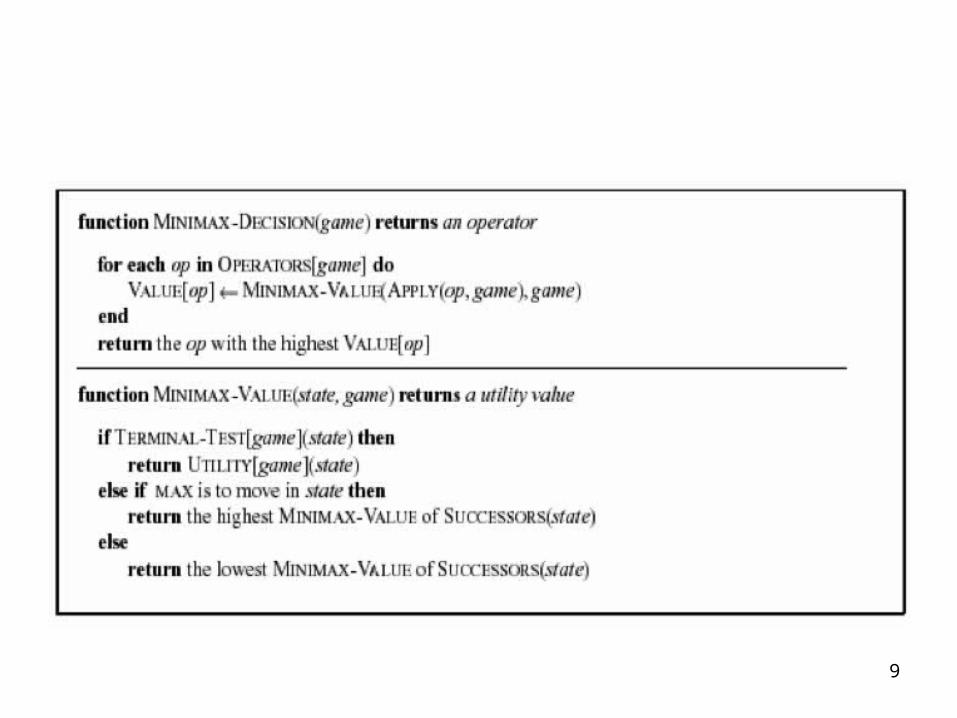
Minimax

• Perfect play for deterministic games

• Idea: choose move to position with highest minimax value = best achievable payoff against best play

• E.g., 2-ply game: [will go through another eg in lecture]

••

•

7

Minimax. Example

8

9

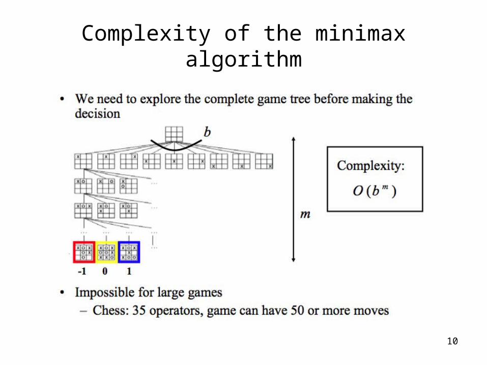
Complexity of the minimax algorithm

10

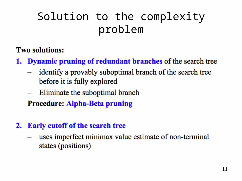
Solution to the complexity problem

11

Alpha Beta Pruning

• Some branches will never be played by rational players since they include sub-optimal decisions for either player

• First, we will see the idea of Alpha Beta Pruning• Then, we’ll introduce the algorithm for minimax with

alpha beta pruning, and go through the example again, showing the book-keeping it does as it goes along

12

Alpha beta pruning. Example

13

Minimax with alpha-beta pruning: The algorithm

• Maxv: function called for max nodes– Might update alpha, the best max can do far

• Minv: function called for min nodes– Might update beta, the best min can do so far

• Each tests for the appropriate pruning case• We’ll go through the algorithm on the course website

14

Algorithm example: alphas/betas shown

15

Properties of α-β

• Pruning does not affect final result

• Good move ordering improves effectiveness of pruning

• With "perfect ordering," time complexity = O(bm/2) doubles depth of search

• A simple example of the value of reasoning about which computations are relevant (a form of metareasoning)

••

•

16

17

Design of evaluation functions

18

Further extensions to real games

19