Advancing Marine Renewable

Energy Monitoring Capabilities

James Joslin

Northwest National Marine Renewable Energy Center

University of Washington

Final Exam

May 7, 2015

Project Motivation

Sustainable development of marine renewable energy

OpenHydro turbine at EMEC Principle Power WindFloat

Ocean Renewable Power Company

RivGen

Columbia Power Technology

SeaRay

2

Environmental Effects

Interactions between stressors and receptors that results

in a detectable or measurable change of biological

importance.

ReceptorStressor

Change

Negative effect

Impact

Positive effect

Benefit

3

Monitoring Wish List

• Spatially comprehensive and temporally continuous

monitoring

• Species level identification of marine animals without

behavioral changes

• Adaptable for evolving monitoring missions

• Survivable in energetic conditions

• Low cost, of course!

Fundy Advanced Sensor

Technology (FAST) Platform

EMEC ReDAPT

4

FLOWBEC

Instrumentation

AVT Manta Optical

Cameras BlueView Acoustical

Camera

icListen HF

Hydrophones

Kongsberg M3

SonarExcelitas Strobes

C-POD Click

Detector

Vemco Fish Tag

Receiver

Nortek Signature

ADCP

5

The Adaptable Monitoring Package

Strobe

Optical

Cameras

Acoustical

Camera

C-POD

Vemco

Hydrophones

ADCP

Securement

Assembly

Recovery

Float

6

Cabled Instrumentation

Mechanical Design by Andy Stewart, Ben Rush and

Paul Gibbs of APL

Seafloor Mounted

Docking Station

“Socket”

AMP

“Plug”

7

ROV Deployment

AMP and

Deployment ROV

Launch

Platform

Load

Bearing

Umbilical

Current Direction

ROV

UmbilicalCabled Docking

Station

RV Jack Robertson

8

Deployment Field Trials

Field trials at Shilshole Marina, February 2015

9

Research Questions

• Optical monitoring subsystem:

• Capabilities at marine energy sites?

• Spacing and layout constraints?

• Endurance for long-term deployments?

• Hydrodynamic analysis:

• Added mass and drag coefficients?

• Stability in turbulent currents?

AMP

Falcon ROV

Millennium Tool

Skid

Docking Station

10

Prototype Camera System

Hybrid Stereo-Optical and Acoustical

Camera System

2 Optical cameras

4 Strobes

BlueView Acoustic

Camera

Main Electronics

Bottle

11

Stereo Optical Tracking

12

Field Testing

Field deployment images with measurement

target corners marked in red

Stereo triangulation measurements

of a target of known size.

Field test frame with camera system

on deck of RV Jack Robertson

13

Optical System Performance SummaryField deployment results show good target visualization

within 4 m.

Camera-Target Separation Distance

Detection Discrimination Classification

2.5 m

Small and large fish Small and large fish Small and large fish

3.5 m

Small and large fish Small and large fish Large fish only

4.5 m

Large fish only Large fish only Unlikely for any fish

14

Capabilities: Endurance Test Imagery

Endurance test video of a seal in a school of fish

15

Optical vs. Acoustical Monitoring

Simultaneous acoustical and optical images from field tests

16

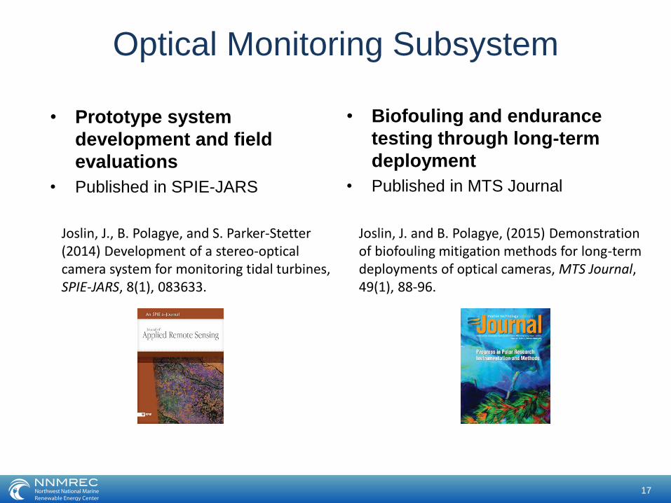
Optical Monitoring Subsystem

17

• Biofouling and endurance

testing through long-term

deployment

• Published in MTS Journal

Joslin, J. and B. Polagye, (2015) Demonstration of biofouling mitigation methods for long-term deployments of optical cameras, MTS Journal, 49(1), 88-96.

• Prototype system

development and field

evaluations

• Published in SPIE-JARS

Joslin, J., B. Polagye, and S. Parker-Stetter (2014) Development of a stereo-optical camera system for monitoring tidal turbines, SPIE-JARS, 8(1), 083633.

Hydrodynamic Analysis• Question: Can an “inspection”-class ROV deploy the AMP in currents

typical of marine energy sites?

• Motivation:

• Lower cost (>10x) than “work”-class ROVs

• Thrust limitations require design optimization

• Methods:

• Drag and added mass coefficient determination

• Dynamic stability analysis

SeaEye’s largest (Jaguar on right) and smallest (Falcon on left) ROVs

18

Loading Conditions

Deployments

• Currents that allow for regular

maintenance < 0.7 m/s

Operations

• Site extremes

< 5.4 m/s

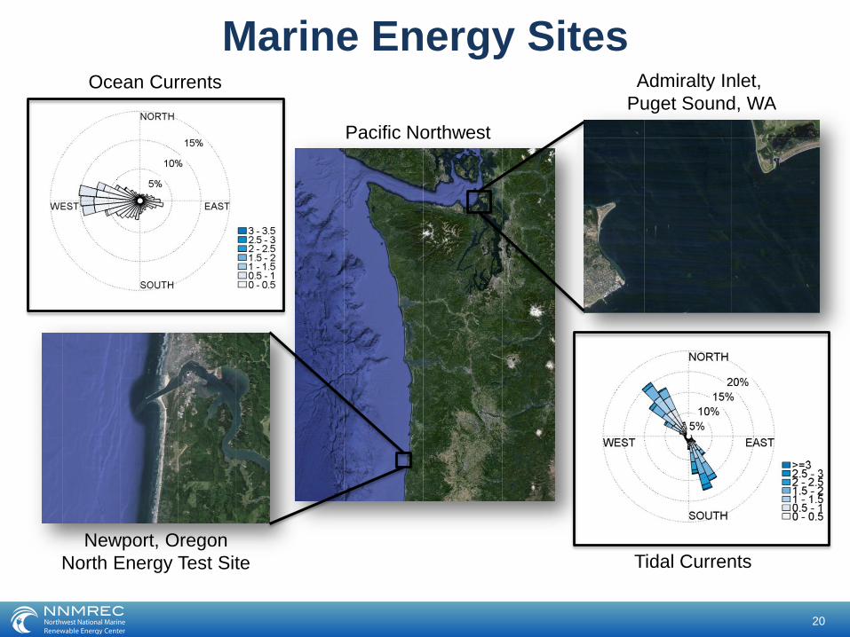
Pacific Northwest

Marine Energy Sites

Tidal Currents

Admiralty Inlet,

Puget Sound, WA

Newport, Oregon

North Energy Test Site

Ocean Currents

20

Underwater Vehicle Dynamics

• 6 degrees of freedom

– Passive control on pitch and roll

– Thruster controlled surge, sway, heave,

and yaw

• Thrusters:

– 8 horizontal

– 2 vertical

• Primary forces and centers:

– Added mass and drag – CoP

– Gravity - CoM

– Buoyancy - CoB

– Thrust - CoT

21

Simulation model free body diagram

TGDC FFFFvM

• Dynamic equation of motion for marine robotics:

ROV Equations of Motion

R6x1

Inertial Forces

0CF

Coriolis and

Centripetal

Drag

Gravity and

Buoyancy

Thrust

Txxxdxxxax FvvCAvmm 2

10

• Simplified equation for translation on a single axis:

Added Mass Drag Coefficient

22

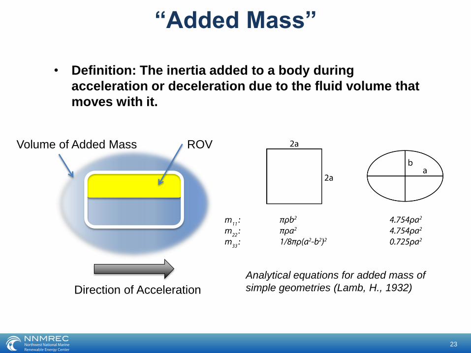
“Added Mass”

• Definition: The inertia added to a body during

acceleration or deceleration due to the fluid volume that

moves with it.

Analytical equations for added mass of

simple geometries (Lamb, H., 1932)

Volume of Added Mass ROV

Direction of Acceleration

23

CFD Simulations

Model free body diagram

• Steady-state simulations to determine lift

and drag coefficients and center of

pressure

• Unstructured tetrahedral mesh with the k-ω

SST turbulence model.

• CFD sensitivity studies:

• Meshing refinements: Coarse, Medium, and

Fine

• Input velocity: 0.1 m/s to 3 m/s

ANSYS fluid domain meshing

Cl 2Fl AU2

Cd 2Fd AU 2

24

Sample CFD Results

Normalized velocity around AMP during

mounted operationNormalized velocity around the Millennium

Falcon and AMP during deployments

• Sensitivity study variability in drag force:• Grid dependence: < 3.50%

• Velocity dependence: < 1.1%

25

Informing Design through CFDCase study of design improvement analysis through CFD:

Drag forces in 5 m/s side-on currents: up to 3150 lbf!

Drag forces and coefficients on

AMP Components

Cd = 0.62

Cd = 1.76

Cd = 1.87

0

2

4

6

8

10

12

14

16

Fixed Strut Farings

Dra

g Fo

rce

[kN

]

Struts

Strobes

AMPBody

AMP with fixed strut fairings

26

Informing Design through CFDCase study of design improvement analysis through CFD:

Rotating struts reduces drag forces by 54% (1400 lbf)

AMP with rotating strut fairings

Drag forces and coefficients on

AMP Components

Cd = 0.62 Cd = 0.48

Cd = 1.76

Cd = 1.04

Cd = 1.87

Cd = 0.57

0

2

4

6

8

10

12

14

16

Fixed Fairings Rotating Fairings

Dra

g Fo

rce

[kN

]

Struts

Strobes

AMP Body

27

CFD Drag Force Results Summary

AMP components Drag forces and coefficients of the AMP by

component

Cd = 0.49 Cd = 0.44

Cd = 0.53Cd = 0.53

Cd = 0.52Cd = 0.52

Cd = 0.79

Cd = 0.76

0.00

0.05

0.10

0.15

0.20

0.25

0.30

0.35

MF with AMP duringDeployment

AMP during MountedOperation

Dra

g Fo

rce

[kN

]

Millennium

Falcon

Struts

Strobes

AMP Body

• Drag coefficient during deployments: Cd ≅ 0.67

• Peak loads during mounted operations:

• Horizontal: 7,880 N

• Vertical: 608 N

28

Experimental Coefficient Measurements• Goal: Verify CFD drag coefficients and measure added mass coefficients

• Methods: Free-decay pendulum experiments

• Benchmark geometries

• ¼ scale models

• Full scale ROV

Ohmsett Tow Tank Facility

Falcon ROV

¼ scale model

6” cube 8.5” sphere

29

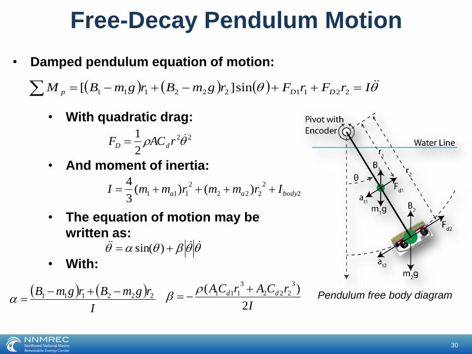
• Damped pendulum equation of motion:

Free-Decay Pendulum Motion

IrFrFrgmBrgmBM DDp 2211222111 sin][

Pendulum free body diagramI

rCArCA dd

2

)(3

222

3

111

I

rgmBrgmB 222111

• With:

)sin(

• The equation of motion may be

written as:

2

2

222

2

111 )()(3

4bodyaa IrmmrmmI

• And moment of inertia:

22

2

1 rACF dD

• With quadratic drag:

30

Pendulum Free-Decay Motion

Pendulum test setup in the

Oceanography test tank

• Incremental angular encoder to

measure pendulum angular

position

• Labview interface to record

encoder data and time

¼ scale ROV mounted to pendulum arm

31

• Collect 10 swings for each

case

• Limit data window by

velocity

• Spline fit to encoder data

• 1st and 2nd order

differentiation for velocity

and acceleration

• Least squares regression

to estimate α and β

Pendulum Data Analysis

Sample data from individual sphere swing

32

• Test data processing

method with synthetic data

set and artificial noise

• Quantize data to simulate

encoder output

• Add initial decaying off axis

oscillations

• Add Gaussian noise

• Added mass +6%

• Drag coefficient +3%

Synthetic Pendulum Data

Synthetic data with artificial noise

33

Benchmark Geometries

• Cube Results:

𝐶𝑑 = 0.690

𝐶𝑑 = 1.05

𝑚𝑎 = 0.7𝜌𝑎3 = 2.4 𝑘𝑔

𝐶𝑑 = 0.723 ± 0.035

𝑚𝑎 = 2.86 ± 0.35

𝐶𝑑 = 0.197

• Sphere Results:

𝐶𝑑 = 0.20

𝑚𝑎 =2

3𝜌𝜋𝑟3 = 2.7 𝑘𝑔

𝐶𝑑 = 0.217 ± 0.015

𝑚𝑎 = 2.62 ± 0.34

34

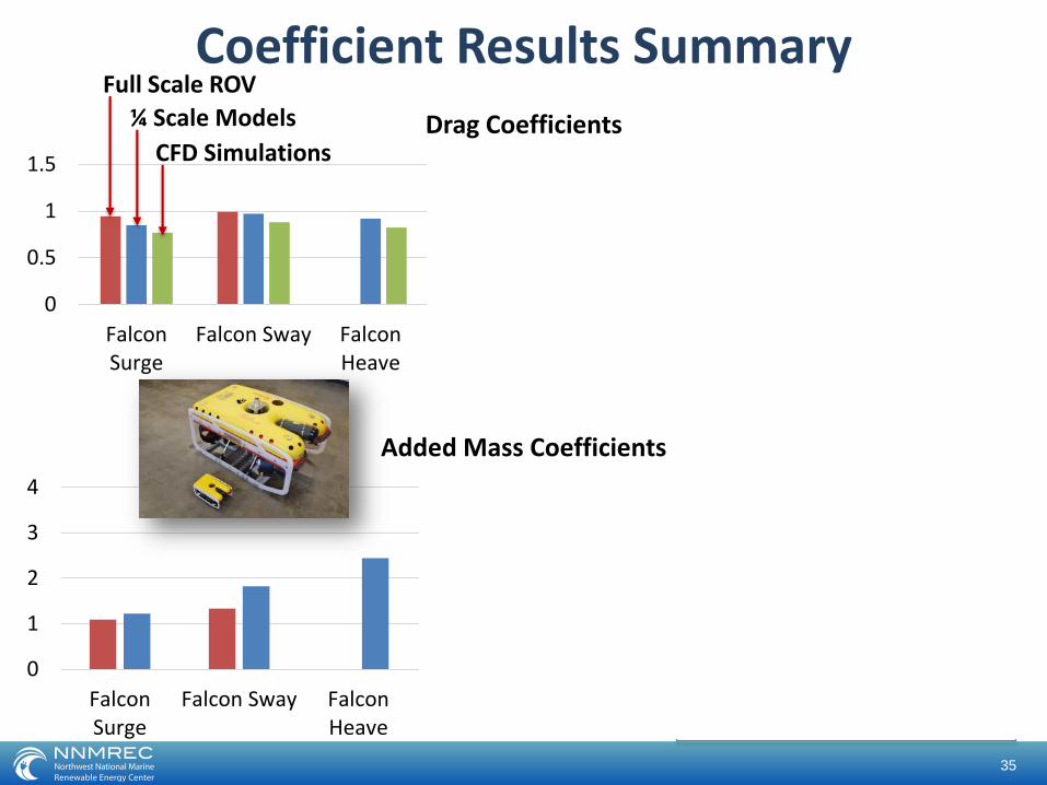
Coefficient Results Summary

0

0.5

1

1.5

FalconSurge

Falcon Sway FalconHeave

AMP Surge AMP Sway MFwASurge

MFwA Sway MFwAHeave

Drag Coefficients

0

1

2

3

4

FalconSurge

Falcon Sway FalconHeave

AMP Surge AMP Sway MFwASurge

MFwA Sway MFwAHeave

Added Mass Coefficients

Full Scale ROV

¼ Scale Models

CFD Simulations

35

AMP and

Deployment ROV

Launch

Platform

Load

Bearing

Umbilical

Current Direction

ROV

UmbilicalCabled Docking

Station

RV Jack Robertson

Dynamic Stability Analysis

Goal: Determine the stability limits for

system operation in the turbulent

currents typical of marine energy sites

36

Simulated AMP Deployment

Dynamic simulation of AMP deployment from an anchored vessel with a launch platform in 1

m waves and 0.7 m/s mean turbulent currents (4x speed)

37

Dynamic Simulations

• ProteusDS: Time-domain dynamic simulator

• System model:

• Surface mesh from simplified solid model

• Inputs variables: Ca, Cd, m, B, I, FTmax, and

centers of mass, buoyancy, and thrust

• Fluid forces: Drag and added mass forces

summed for relative fluid motion on each surface

polygon

• Limitations:

• No fluid interaction calculations

• Simplified hydrodynamic coefficients

• Simplified thruster dynamics

Simulation model free body diagram

𝑓𝑑 =1

2𝜌𝐶𝑑𝐴𝑝𝑟𝑜𝑗𝑣

2 𝑓𝑖 = 𝜌𝐶𝑎𝑉𝑑𝑖𝑠𝑝 𝑣

38

Hydrodynamic Model Verification

• Dynamic simulations of free-decay pendulum

experiments to verify hydrodynamic

coefficients:

Simulated pendulum motion Free-decay pendulum experiment

ProteusDS model

39

Hydrodynamic Model Validation

• Comparison of simulation and experimental results:

Simulated pendulum experiments

40

Admiralty Inlet turbulent current data

Turbulent Current Forcing

• Data from tidal turbulence mooring deployment in Admiralty

Inlet

• Corrected for mooring motion

• Split into 5 minute bursts for

consistent mean velocity

• Binned by mean velocity: 0 to

1.1 m/s

• Low-pass filter u, v, and w

components to constitute

“engulfing gusts”

• Where L = 1.5 is the system

length scale

𝑓𝑐 = 𝑢

𝐿

41

u

v

w

y-z

plane

Δx

Turbulent Current Forcing

• 5 minute ADV files used to generate time-varying 3D current

fields

• Define grid of y-z planes spaced

by Δx = 1 m

• Assign u, v, and w current

components to y-z planes

• Propagate turbulence

downstream at mean current

velocity

• ProteusDS linearly interpolates

between planes and over time

Time-varying “3D” current forcing

42

Simulated Operations

• Simplified deployment operations with system driving against

the turbulent current forcing

Simulation with umbilical (4x speed),

Run time = 47 hrs

Simulation without umbilical (4x speed),

Run time = 0.5 hrs

43

Navigation Controllers

• PID controllers for:

• Yaw (heading)

• Surge (forward velocity)

• Heave (depth)

• Simulate thruster forces

at centers of thrust

• Limited to ROV thrust

capacity

• Horizontal thrust limit = 70

kgf

• Vertical thrust limit = 22 kgf

Representative simulation data for surge

controller

44

ROV Thrust Capacity

• Horizontal thrust is the sum of the yaw torque and surge force

Representative controller thrust forces for 0.5 and 0.8 m/s mean currents

45

Horizontal thrust allocation to yaw and surge

Operational Limits

• Limit determined by a 5% threshold for thrusters operating at

capacity

Thruster time operating at capacity for simulations

without the umbilical

• Predicted limits:

- 0.75 m/s without umbilical

- 0.74 m/s with umbilical

• Thrust allocation:

- Without umbilical: 21% yaw, 79% surge

- With umbilical: 19% yaw, 81% surge

46

Passive Stability

• Pitch and roll stability maintained by buoyant righting moment

Passive stability from simulations without the umbilical

• Less than ± 0.5° roll at

the operational limit

• 3.3° forward pitch due

to offset between

centers of thrust and

pressure

47

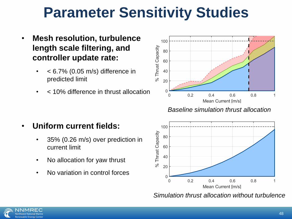
Parameter Sensitivity Studies

• Mesh resolution, turbulence

length scale filtering, and

controller update rate:

• < 6.7% (0.05 m/s) difference in

predicted limit

• < 10% difference in thrust allocation

Baseline simulation thrust allocation

Simulation thrust allocation without turbulence

• Uniform current fields:

• 35% (0.26 m/s) over prediction in

current limit

• No allocation for yaw thrust

• No variation in control forces

48

Baseline simulation thrust allocation

Simulation thrust allocation

Simulation thrust allocation

Parameter Sensitivity Studies

• Hydrodynamic coefficients:

• Measured values

• CFD estimates (drag only)

• Canonical values

• Canonical Values:

• 11% (0.08 m/s) increased limit

• Under predicted yaw control and

variation

• Worst Case:

• CFD for drag and canonical

values for added mass

• 25% (0.19 m/s) increased limit

• Under predicted yaw control and

variation

49

Dynamic Analysis Conclusions

• Deployment limit of 0.7 m/s

• “Inspection”-class ROV operations at marine energy sites

• Turbulence effects are non-negligible in these environments

• Hydrodynamic coefficients measurements through free-decay

pendulum motion

• 2 pending publications

Joslin, J., B. Polagye, A. Stewart, and B. Fabien (in prep) Dynamic Simulation of a Remotely-operated Underwater Vehicle in Turbulent Currents for Marine Energy Applications.

Joslin, J., B. Polagye, and A. Stewart(in review) Hydrodynamic coefficient determination for an open-framed underwater vehicle, J. Ocean Eng.

50

Summary• AMP and Millennium Falcon development

• Optical monitoring capabilities for marine energy converters

• Hydrodynamic coefficient measurements

• Dynamic stability and operational limits in turbulent currents

System Deployment from the R/V Jack Robertson

51

What’s Next?• AMP and Millennium Falcon field testing

• Instrument integration and algorithm development

• Autonomous deployment capabilities

• Benchmarking simulated performance against field performance

• MarineSitu spin off to provide marine monitoring services to

industry developers

MARINESITU

52

Acknowledgements

This material is based upon work supported by the Department of Energy under FG36-08GO18179-M001, Snohomish Public Utility District, and the Naval Facilities Engineering Command.

Thank you to my colleagues, friends, and family who have

supported me throughout grad school.

Special thanks to my committee:

Brian Polagye

Brian Fabien

Andy Stewart

Jim Thomson

Alex Horner-Devine

Thank You

Questions?