Embed Size (px)
DESCRIPTION
Advances inHigh-PerformanceMotion Control ofMechatronic Systems
Citation preview

6000 Broken Sound Parkway, NW Suite 300, Boca Raton, FL 33487711 Third Avenue New York, NY 100172 Park Square, Milton Park Abingdon, Oxon OX14 4RN, UK
an informa business
www.crcpress.com w w w . c r c p r e s s . c o m
K15386
ENVIRONMENTAL SCIENCE
Advances in H
igh-Perform
ance Motion C
ontrol of Mechatronic S
ystems
Yamaguchi • H
irata • Pang
Edited byTakashi YamaguchiMitsuo HirataChee Khiang Pang
Advances in
High-PerformanceMotion Control ofMechatronic Systems
Advances in
High-Performance Motion Control ofMechatronic Systems

Advances in
High-PerformanceMotion Control ofMechatronic Systems
K15386_FM.indd 3 6/27/13 2:17 PM


Boca Raton London New York
CRC Press is an imprint of theTaylor & Francis Group, an informa business
Edited byTakashi YamaguchiMitsuo HirataChee Khiang Pang
Advances in
High-PerformanceMotion Control ofMechatronic Systems
K15386_FM.indd 3 6/27/13 2:17 PM

MATLAB® is a trademark of The MathWorks, Inc. and is used with permission. The MathWorks does not warrant the accuracy of the text or exercises in this book. This book’s use or discussion of MATLAB® soft-ware or related products does not constitute endorsement or sponsorship by The MathWorks of a particular pedagogical approach or particular use of the MATLAB® software.
CRC PressTaylor & Francis Group6000 Broken Sound Parkway NW, Suite 300Boca Raton, FL 33487-2742
© 2014 by Taylor & Francis Group, LLCCRC Press is an imprint of Taylor & Francis Group, an Informa business
No claim to original U.S. Government worksVersion Date: 20130619
International Standard Book Number-13: 978-1-4665-5571-6 (eBook - PDF)
This book contains information obtained from authentic and highly regarded sources. Reasonable efforts have been made to publish reliable data and information, but the author and publisher cannot assume responsibility for the validity of all materials or the consequences of their use. The authors and publishers have attempted to trace the copyright holders of all material reproduced in this publication and apologize to copyright holders if permission to publish in this form has not been obtained. If any copyright material has not been acknowledged please write and let us know so we may rectify in any future reprint.
Except as permitted under U.S. Copyright Law, no part of this book may be reprinted, reproduced, transmit-ted, or utilized in any form by any electronic, mechanical, or other means, now known or hereafter invented, including photocopying, microfilming, and recording, or in any information storage or retrieval system, without written permission from the publishers.
For permission to photocopy or use material electronically from this work, please access www.copyright.com (http://www.copyright.com/) or contact the Copyright Clearance Center, Inc. (CCC), 222 Rosewood Drive, Danvers, MA 01923, 978-750-8400. CCC is a not-for-profit organization that provides licenses and registration for a variety of users. For organizations that have been granted a photocopy license by the CCC, a separate system of payment has been arranged.
Trademark Notice: Product or corporate names may be trademarks or registered trademarks, and are used only for identification and explanation without intent to infringe.
Visit the Taylor & Francis Web site athttp://www.taylorandfrancis.com
and the CRC Press Web site athttp://www.crcpress.com

To my family, and my colleagues who have worked with us forcontinuous improvements in mechatronics servo control.
T. Yamaguchi
To my parents, my wife, and my two sons.
M. Hirata
To those who believe in me, and those who look down on me.
C. K. Pang


Contents
List of Figures xiii
List of Tables xxiii
Preface xxv
Editors’ Biographies xxix
Contributors xxxi
1 Introduction to High-Performance Motion Control of Mecha-tronic Systems 1
T. Yamaguchi1.1 Concept of Advances in High-Performance Motion Control of
Mechatronic Systems . . . . . . . . . . . . . . . . . . . . . . 11.1.1 Scope of Book . . . . . . . . . . . . . . . . . . . . . . 11.1.2 Past Studies from High-Speed Precision Motion Control 4
1.2 Hard Disk Drives (HDDs) as a Classic Example . . . . . . . 51.2.1 Mechanical Structure . . . . . . . . . . . . . . . . . . 51.2.2 Modeling . . . . . . . . . . . . . . . . . . . . . . . . . 6
1.3 Brief History of HDD and Its Servo Control . . . . . . . . . 81.3.1 Growth in Areal Density . . . . . . . . . . . . . . . . . 81.3.2 Technological Development in Servo Control . . . . . . 10
1.3.2.1 Application of Control Theories . . . . . . . 101.3.2.2 Improvement of Control Structure . . . . . . 12
Bibliography 13
2 Fast Motion Control Using TDOF Control Structure and Op-timal Feedforward Input 17
M. Hirata2.1 TDOF Control Structure . . . . . . . . . . . . . . . . . . . . 18
2.1.1 One-Degree-Of-Freedom Control System . . . . . . . . 182.1.2 Two-Degrees-Of-Freedom Control System . . . . . . . 192.1.3 Implementation of Feedforward Input by TDOF Control
Structure . . . . . . . . . . . . . . . . . . . . . . . . . 222.2 Optimum Feedforward Input Design . . . . . . . . . . . . . . 23
vii

viii
2.2.1 Minimum Time Control . . . . . . . . . . . . . . . . . 232.2.2 Minimum Jerk Input . . . . . . . . . . . . . . . . . . . 242.2.3 Digital Implementation of Minimum Jerk Input . . . . 272.2.4 Sampled-Data Polynomial Input . . . . . . . . . . . . 28
2.3 Final-State Control . . . . . . . . . . . . . . . . . . . . . . . 332.3.1 Problem Formulation . . . . . . . . . . . . . . . . . . 332.3.2 Minimum Jerk Input Design by FSC . . . . . . . . . . 342.3.3 Vibration Minimized Input Design by FSC . . . . . . 352.3.4 Final-State Control with Constraints . . . . . . . . . . 38
2.4 Industrial Application: Hard Disk Drives . . . . . . . . . . . 392.4.1 HDD Benchmark Problem and the Plant Model . . . . 392.4.2 FSC and FFSC Inputs Design . . . . . . . . . . . . . . 42
2.5 Industrial Application: Galvano Scanner I . . . . . . . . . . . 482.5.1 Plant Model . . . . . . . . . . . . . . . . . . . . . . . . 482.5.2 FSC and FFSC Inputs Design . . . . . . . . . . . . . . 492.5.3 Simulation Results . . . . . . . . . . . . . . . . . . . . 532.5.4 Experimental Results . . . . . . . . . . . . . . . . . . 54
2.6 Industrial Application: Galvano Scanner II . . . . . . . . . . 582.6.1 Voltage Saturation in Current Amplifier . . . . . . . . 582.6.2 FSC Design Considering Voltage Saturation in Current
Amplifier . . . . . . . . . . . . . . . . . . . . . . . . . 592.6.3 Application to Galvano Scanner Control Problem . . . 61
Bibliography 67
3 Transient Control Using Initial Value Compensation 69
A. Okuyama, N. Hirose, T. Yamaguchi, and M. Iwasaki3.1 Introduction . . . . . . . . . . . . . . . . . . . . . . . . . . . 70
3.1.1 Background . . . . . . . . . . . . . . . . . . . . . . . . 703.1.2 Initial Value Compensation (IVC) . . . . . . . . . . . 73
3.2 Overview of Switching Control . . . . . . . . . . . . . . . . . 743.3 Design of IVC . . . . . . . . . . . . . . . . . . . . . . . . . . 78
3.3.1 Design of Initial Values on Feedback Controller . . . . 793.3.2 Design of Additional Input to Controller . . . . . . . . 843.3.3 Design of Optimal Switching Condition . . . . . . . . 89
3.4 Industrial Applications 1 (IVC for Mode Switching) . . . . . 973.4.1 HDD (Reduction of Acoustic Noise) . . . . . . . . . . 973.4.2 Robot (Personal Mobility Robot) . . . . . . . . . . . . 100
3.4.2.1 Introduction . . . . . . . . . . . . . . . . . . 1003.4.2.2 Mathematical Model . . . . . . . . . . . . . . 1103.4.2.3 Design of IVC . . . . . . . . . . . . . . . . . 1113.4.2.4 Experimental Results . . . . . . . . . . . . . 112
3.4.3 Optical Disk Drive . . . . . . . . . . . . . . . . . . . . 1133.5 Industrial Applications 2 (IVC for reference switching) . . . 114
3.5.1 Galvano Mirror for Laser Drilling Machine . . . . . . 114
ix
3.5.1.1 Introduction . . . . . . . . . . . . . . . . . . 1143.5.1.2 Mathematical Model . . . . . . . . . . . . . . 1153.5.1.3 Design of IVC . . . . . . . . . . . . . . . . . 1233.5.1.4 Experimental Results . . . . . . . . . . . . . 123
3.6 Conclusion . . . . . . . . . . . . . . . . . . . . . . . . . . . . 123
Bibliography 129
4 Precise Positioning Control in Sampled-Data Systems 135
T. Atsumi4.1 Introduction . . . . . . . . . . . . . . . . . . . . . . . . . . . 1364.2 Sensitivity and Complementary Sensitivity Transfer Functions
in Sampled-Data Control Systems . . . . . . . . . . . . . . . 1374.2.1 Relationship Between Continuous- and Discrete-Time
Signals . . . . . . . . . . . . . . . . . . . . . . . . . . . 1374.2.2 Sensitivity and Complementary Sensitivity Transfer
Functions in Sampled-Data Control Systems . . . . . 1384.2.3 Sampled-Data Control System Using a Multi-Rate Dig-
ital Filter . . . . . . . . . . . . . . . . . . . . . . . . . 1424.3 Unobservable Oscillations in Sampled-Data Positioning Sys-
tems . . . . . . . . . . . . . . . . . . . . . . . . . . . . . . . . 1464.3.1 Relationship Between Oscillation Frequency and Unob-
servable Magnitude of Oscillations . . . . . . . . . . . 1464.3.1.1 Definition of Unobservable Magnitude of Os-
cillations . . . . . . . . . . . . . . . . . . . . 1464.3.1.2 Oscillations at the Sampling Frequency . . . 1474.3.1.3 Oscillations at the Nyquist Frequency . . . . 1484.3.1.4 Oscillations at One-Third of the Sampling Fre-
quency . . . . . . . . . . . . . . . . . . . . . 1504.3.2 Unobservable Magnitudes of Oscillations with Damping 150
4.3.2.1 Definition of Unobservable Magnitudes of Os-cillations with Damping . . . . . . . . . . . . 150
4.3.2.2 Example of Unobservable Magnitudes for Os-cillations with Damping . . . . . . . . . . . . 152
4.3.2.3 Index of Unobservable Magnitudes . . . . . . 1574.4 Residual Vibrations in Sampled-Data Positioning Control Sys-
tems . . . . . . . . . . . . . . . . . . . . . . . . . . . . . . . . 1624.4.1 Residual Vibration Analysis Based on SRS Analysis . 162
4.4.1.1 SRS Analysis . . . . . . . . . . . . . . . . . . 1624.4.1.2 SRS Analysis Using Half-Sine Wave . . . . . 1644.4.1.3 SRS Analysis Using Polynomial Wave . . . . 1664.4.1.4 Comparison between SRS and DFT . . . . . 168
4.5 Hard Disk Drive Example . . . . . . . . . . . . . . . . . . . . 1754.5.1 Head-Positioning Control System . . . . . . . . . . . . 175
4.5.1.1 Controlled Object . . . . . . . . . . . . . . . 176
x
4.5.2 Sensitivity and Complementary Sensitivity TransferFunctions . . . . . . . . . . . . . . . . . . . . . . . . . 1774.5.2.1 Design of Control System . . . . . . . . . . . 1784.5.2.2 Simulation and Experiment . . . . . . . . . . 180
4.5.3 Unobservable Oscillations . . . . . . . . . . . . . . . . 1874.5.4 Residual Vibrations . . . . . . . . . . . . . . . . . . . 188
4.5.4.1 Feedback Control System . . . . . . . . . . . 1894.5.4.2 Feedforward Control System . . . . . . . . . 1914.5.4.3 SRS Analysis . . . . . . . . . . . . . . . . . . 1924.5.4.4 Simulation and Experimental Results . . . . 193
Bibliography 197
5 Dual-Stage Systems and Control 199
C. K. Pang, F. Hong, and M. Nagashima5.1 Introduction . . . . . . . . . . . . . . . . . . . . . . . . . . . 2005.2 System Identification of Dual-Stage Actuators in HDDs . . . 201
5.2.1 Primary Actuator: VCM . . . . . . . . . . . . . . . . . 2025.2.1.1 Continuous-Time Measurement . . . . . . . . 2025.2.1.2 Discrete-Time Measurement . . . . . . . . . 203
5.2.2 Secondary Actuator: PZT Active Suspension . . . . . 2105.2.2.1 Continuous-Time Measurement . . . . . . . . 2105.2.2.2 Discrete-Time Measurement . . . . . . . . . 212
5.3 Resonance Compensation Without Extraneous Sensors . . . 2135.3.1 Gain Stabilization . . . . . . . . . . . . . . . . . . . . 2145.3.2 Inverse Compensation . . . . . . . . . . . . . . . . . . 2145.3.3 Phase Stabilization . . . . . . . . . . . . . . . . . . . . 215
5.3.3.1 Using Mechanical Resonant Modes . . . . . . 2155.3.3.2 Using LTI Peak Filters . . . . . . . . . . . . 2165.3.3.3 Using LTV Peak Filters . . . . . . . . . . . . 224
5.3.4 Experimental Verifications . . . . . . . . . . . . . . . . 2275.4 Resonance Compensation With Extraneous Sensors . . . . . 230
5.4.1 Active Damping . . . . . . . . . . . . . . . . . . . . . 2315.4.2 Self-Sensing Actuation (SSA) . . . . . . . . . . . . . . 231
5.4.2.1 Direct-Driven SSA (DDSSA) . . . . . . . . . 2325.4.2.2 Indirect-Driven SSA (IDSSA) . . . . . . . . . 234
5.4.3 Model-Based Design . . . . . . . . . . . . . . . . . . . 2355.4.4 Non-Model-Based Design . . . . . . . . . . . . . . . . 238
5.5 Dual-Stage Controller Design . . . . . . . . . . . . . . . . . . 2425.5.1 Control Structure . . . . . . . . . . . . . . . . . . . . . 243
5.5.1.1 Parallel . . . . . . . . . . . . . . . . . . . . . 2435.5.1.2 Coupled Master-Slave (CMS) . . . . . . . . . 2445.5.1.3 Decoupled Master-Slave (DMS) . . . . . . . 245
5.5.2 Design Example . . . . . . . . . . . . . . . . . . . . . 2465.5.2.1 Primary Actuator Controller: VCM Loop . . 247

xi
5.5.2.2 Secondary Actuator Controller: PZT ActiveSuspension Loop . . . . . . . . . . . . . . . . 248
5.5.3 Simulation Results . . . . . . . . . . . . . . . . . . . . 2505.6 Conclusion . . . . . . . . . . . . . . . . . . . . . . . . . . . . 252
Bibliography 253
6 Concluding Remarks from Editors 259
T. Yamaguchi, M. Hirata, and C. K. Pang6.1 Transferring Technologies to Other Industries (T. Yamaguchi) 260
6.1.1 What is High-Speed Precision Motion Control? . . . . 2606.1.2 Sensing and Closing the Loop: Shifting Resource Power
to a Right Field . . . . . . . . . . . . . . . . . . . . . 2616.1.3 Control Structure: Generating New Design Parameters 2626.1.4 Modeling: Necessity of Precise Disturbance Modeling . 2636.1.5 Summary . . . . . . . . . . . . . . . . . . . . . . . . . 263
6.2 What Can We Do when the Positioning Accuracy Reaches aLimit? (M. Hirata) . . . . . . . . . . . . . . . . . . . . . . . 2676.2.1 Motivation . . . . . . . . . . . . . . . . . . . . . . . . 2676.2.2 Support Vector Machine . . . . . . . . . . . . . . . . . 2676.2.3 Application to the Head-Positioning Control Problem
in HDDs . . . . . . . . . . . . . . . . . . . . . . . . . . 2696.2.3.1 Approach . . . . . . . . . . . . . . . . . . . . 2696.2.3.2 Plant Model . . . . . . . . . . . . . . . . . . 2696.2.3.3 Training the Discriminant Function . . . . . 2706.2.3.4 Validation . . . . . . . . . . . . . . . . . . . 271
6.2.4 Summary . . . . . . . . . . . . . . . . . . . . . . . . . 2726.3 Control Constraints and Specifications (C. K. Pang) . . . . . 274
6.3.1 Constraints and Limitations . . . . . . . . . . . . . . . 2746.3.1.1 Anti-Resonant Zeros . . . . . . . . . . . . . . 2766.3.1.2 Resonant Poles . . . . . . . . . . . . . . . . . 2776.3.1.3 Sensitivity Transfer Function . . . . . . . . . 2776.3.1.4 Limitations on Positioning Accuracy . . . . . 278
6.3.2 Bode’s Integral Theorem . . . . . . . . . . . . . . . . . 2796.3.2.1 Continuous Bode’s Integral Theorem . . . . 2796.3.2.2 Discrete Bode’s Integral Theorem . . . . . . 280
6.3.3 Summary . . . . . . . . . . . . . . . . . . . . . . . . . 281
Bibliography 283
Index 285


List of Figures
1.1 Definition of mechatronics [3]. . . . . . . . . . . . . . . . . . 2
1.2 Schematic apparatus of an HDD. . . . . . . . . . . . . . . . 5
1.3 Block diagram of plant model and disturbances in HDDs. . 6
1.4 Frequency response of the nominal model [1]. . . . . . . . . 7
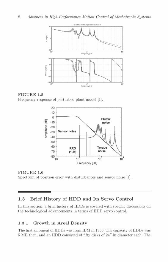
1.5 Frequency response of perturbed plant model [1]. . . . . . . 8
1.6 Spectrum of position error with disturbances and sensornoise [1]. . . . . . . . . . . . . . . . . . . . . . . . . . . . . . 8
1.7 Trend of HDD areal density [4, 5]. . . . . . . . . . . . . . . . 9
1.8 Trend of positioning accuracy in HDDs [6]. . . . . . . . . . . 10
2.1 One-degree-of-freedom control system. . . . . . . . . . . . . 18
2.2 General formulation of two-degrees-of-freedom control system. 19
2.3 ODOF controller in TDOF controller structure. . . . . . . . 19
2.4 Examples of TDOF control systems. . . . . . . . . . . . . . 21
2.5 Implementation of feedforward input by the TDOF controlstructure. . . . . . . . . . . . . . . . . . . . . . . . . . . . . 22
2.6 Implementation of feedforward input when plant has inputdelay. . . . . . . . . . . . . . . . . . . . . . . . . . . . . . . . 23
2.7 Augmented system for minimum jerk input. . . . . . . . . . 24
2.8 Minimum jerk input. . . . . . . . . . . . . . . . . . . . . . . 27
2.9 Digital implementation of umjc(t). . . . . . . . . . . . . . . 27
2.10 Minimum jerk control for different sampling periods. . . . . 28
2.11 Augmented system with a discrete-time integrator. . . . . . 34
2.12 Bode plot of the nominal model. . . . . . . . . . . . . . . . . 41
2.13 Bode plots of the perturbed plants. . . . . . . . . . . . . . . 41
2.14 Design 1: Feedforward input for one track-seek. . . . . . . . 43
2.15 Design 1: Output response for one track-seek. . . . . . . . . 43
2.16 Design 1: Feedforward input for ten track-seek. . . . . . . . 44
2.17 Design 1: Output response for ten track-seek. . . . . . . . . 44
2.18 Design 2: Feedforward input for one track-seek. . . . . . . . 46
2.19 Design 2: Output response for one track-seek. . . . . . . . . 46
2.20 Design 2: Feedforward input for ten track-seek. . . . . . . . 47
2.21 Design 2: Output response for ten track-seek. . . . . . . . . 47
2.22 Control system of galvano scanner. . . . . . . . . . . . . . . 48
2.23 Frequency responses of galvano scanner. . . . . . . . . . . . 49
xiii

xiv Advances in High-Performance Motion Control of Mechatronic Systems
2.24 Augmented system to design the FSC and FFSC inputs forthe galvano scanner. . . . . . . . . . . . . . . . . . . . . . . 51
2.25 Time responses of FSC and FFSC inputs. . . . . . . . . . . 52
2.26 Spectra of FFSC and FSC inputs. . . . . . . . . . . . . . . . 52
2.27 MMTDOF control system for galvano scanner control system. 53
2.28 Simulated time responses of output when the frequency of theprimary vibration mode is changed from −6% to +6%. . . . 53
2.29 Spectra of FSC and FFSC inputs when nominal frequency ofprimary vibration mode is perturbed to +6% of the nominalfrequency in both FSC and FFSC designs. . . . . . . . . . . 55
2.30 Experimental time responses of outputs. . . . . . . . . . . . 56
2.31 Experimental time responses of outputs when nominal fre-quency of primary vibration mode is perturbed to +6% of thenominal frequency in both FSC and FFSC designs. . . . . . 56
2.32 Spectra of residual vibrations when nominal frequency of pri-mary vibration mode is perturbed to +6% of the nominalfrequency. . . . . . . . . . . . . . . . . . . . . . . . . . . . . 57
2.33 Control system with current amplifier. . . . . . . . . . . . . 59
2.34 Augmented system for rigid-body mode model. . . . . . . . 59
2.35 Augmented system for voltage constraint. . . . . . . . . . . 60
2.36 Trajectory waveforms of 1 mm step. . . . . . . . . . . . . . 64
2.37 Position responses of 1 mm step when the FFSC inputs weredesigned without input voltage constraint. . . . . . . . . . . 65
2.38 Position responses of 1 mm step when the FFSC inputs weredesigned with input voltage constraint. . . . . . . . . . . . . 65
2.39 Energy consumption in the current amplifier. . . . . . . . . 66
3.1 Block diagram of a switching control system. . . . . . . . . . 75
3.2 Constrained control system. . . . . . . . . . . . . . . . . . . 76
3.3 Maximal output admissible set. . . . . . . . . . . . . . . . . 77
3.4 Inclusive relationship of maximal output admissible sets. . . 78
3.5 Block diagram of a simplified case of the HDD head-positioning servo system. . . . . . . . . . . . . . . . . . . . . 82
3.6 Transient responses with and without IVC (simulation). . . 82
3.7 Block diagram of HDD head-positioning servo system withtime delay considered. . . . . . . . . . . . . . . . . . . . . . 83
3.8 Transient responses with and without IVC (simulation). . . 83
3.9 Block diagram of control system with additional input r′. . 85
3.10 Transient waveforms for various desired eigenvalues (simula-tion). . . . . . . . . . . . . . . . . . . . . . . . . . . . . . . . 89
3.11 Trajectories on phase plane (simulation). . . . . . . . . . . . 90
3.12 Transient waveforms with IVC compensation (simulations andexperiments). . . . . . . . . . . . . . . . . . . . . . . . . . . 91
3.13 H2-norm plane for initial velocity and acceleration. . . . . . 94
List of Figures xv
3.14 Transient response of head position after mode switching (ex-perimental results). . . . . . . . . . . . . . . . . . . . . . . . 95
3.15 Transient response of current after mode switching (experi-mental results). . . . . . . . . . . . . . . . . . . . . . . . . . 95
3.16 Maximal output admissible sets. . . . . . . . . . . . . . . . . 97
3.17 Simulations results for initialization using IVC. . . . . . . . 101
3.18 Simulation results for initialization using zero reset. . . . . . 102
3.19 Experimental results for initialization using IVC. . . . . . . 103
3.20 Block diagram of model-following control system with IVC. 104
3.21 Initial state sets that meet their individual constraint condi-tion on the current peak value cp. . . . . . . . . . . . . . . . 105
3.22 Initial state sets that meet their individual constraint condi-tion on the overshoot os. . . . . . . . . . . . . . . . . . . . . 106
3.23 Initial state sets that meet their individual constraint condi-tion on the settling time st. . . . . . . . . . . . . . . . . . . 107
3.24 Experimental results for pole-zero-type IVC. . . . . . . . . . 108
3.25 Experimental results for J-min-type IVC. . . . . . . . . . . . 108
3.26 Configuration of prototype PMR. . . . . . . . . . . . . . . . 109
3.27 Transition from four-wheel mode to wheeled inverted pendu-lum mode. . . . . . . . . . . . . . . . . . . . . . . . . . . . . 110
3.28 Model of wheeled inverted pendulum mode of PMR. . . . . 111
3.29 Block diagram of switching control system for making transi-tion between the four-wheel mode and the wheeled invertedpendulum mode. . . . . . . . . . . . . . . . . . . . . . . . . 111
3.30 Experimental results with and without IVC. . . . . . . . . . 117
3.31 Experimental results for acceleration of driver’s head. . . . . 118
3.32 Schematic apparatus of an optical disk drive. . . . . . . . . 118
3.33 Focus servo system of the experimental setup with the high-gain servo controller [32]. . . . . . . . . . . . . . . . . . . . . 119
3.34 Initial responses of the focus servo system of the experimentalsetup without IVC [32]. . . . . . . . . . . . . . . . . . . . . . 119
3.35 Initial responses of the focus servo system of the experimentalsetup with IVC [32]. . . . . . . . . . . . . . . . . . . . . . . 120
3.36 Configuration of experimental setup. . . . . . . . . . . . . . 120
3.37 Frequency response of plant system from iref to ys. . . . . . 121
3.38 Experimental position error responses. . . . . . . . . . . . . 121
3.39 Experimental position error responses for a reference with aninterval period of 1.50 ms. . . . . . . . . . . . . . . . . . . . 122
3.40 Experimental position error responses for a reference with aninterval period of 1.16 ms. . . . . . . . . . . . . . . . . . . . 122
3.41 Pole-zero plots without IVC. . . . . . . . . . . . . . . . . . . 125
3.42 Pole-zero plots with IVC. . . . . . . . . . . . . . . . . . . . . 126
3.43 Experimental position error responses with IVC for a referencewith an interval period of 1.50 ms. . . . . . . . . . . . . . . 127

xvi Advances in High-Performance Motion Control of Mechatronic Systems
3.44 Experimental position error responses with IVC for a referencewith an interval period of 1.16 ms. . . . . . . . . . . . . . . 127
4.1 Block diagram of a sampled-data control system. . . . . . . 1454.2 Block diagram of a sampled-data control system with a multi-
rate filter. . . . . . . . . . . . . . . . . . . . . . . . . . . . . 1454.3 Relationship between maximum unobservable magnitude yuw
and ωt (τ = 25 μs). . . . . . . . . . . . . . . . . . . . . . . . 1474.4 Dependence of unobservable magnitude yu on sampling phase
Δs ∈ [0, 1) for an oscillation at the sampling frequency. . . . 1484.5 Time responses of yc and yd for an oscillation at the sampling
frequency. Solid: yc. ‘o’: yd with Δs = 0. ‘x’: yd with Δs =0.25. . . . . . . . . . . . . . . . . . . . . . . . . . . . . . . . 148
4.6 Unobservable magnitude for an oscillation at the Nyquist fre-quency. . . . . . . . . . . . . . . . . . . . . . . . . . . . . . . 149
4.7 Time responses of yc and yd for an oscillation at the Nyquistfrequency. Solid: yc. ‘o’: yd with Δs = 0.5. ‘x’: yd with Δs = 0. 149
4.8 Unobservable magnitude for an oscillation at one-third of thesampling frequency. . . . . . . . . . . . . . . . . . . . . . . . 150
4.9 Time responses of yc and yd for an oscillation at one-third ofthe sampling frequency. Solid: yc. ‘o’: yd with Δs = 0. ‘x’: ydwith Δs = 0.75. . . . . . . . . . . . . . . . . . . . . . . . . . 151
4.10 Example of time responses of yc and yd with damping for afinite number of samples (Ns = 5). . . . . . . . . . . . . . . 152
4.11 Unobservable magnitude for a damped oscillation at the sam-pling frequency (τ = 25 μs, ζ = 0.1, and Ns = 5). . . . . . . 152
4.12 Time responses of yc and yd for a damped oscillation at thesampling frequency (τ = 25 μs, ζ = 0.1, and Ns = 5). Solid:yc. ‘o’: yd with Δs = 0. ‘x’: yd with Δs = 0.25. . . . . . . . . 153
4.13 Histogram of event probability of unobservable magnitude fora damped oscillation at the sampling frequency (τ = 25 μs, ζ= 0.1, and Ns = 5). . . . . . . . . . . . . . . . . . . . . . . . 153
4.14 Unobservable magnitude for a damped oscillation at theNyquist frequency (τ = 25 μs, ζ = 0.1, and Ns = 5). . . . . 154
4.15 Time responses of yc and yd for a damped oscillation at theNyquist frequency (τ = 25 μs, ζ = 0.1, and Ns = 5). Solid:yc. ‘o’: yd with Δs = 0.5. ‘x’: yd with Δs = 0. . . . . . . . . 154
4.16 Histogram of event probability of unobservable magnitude fora damped oscillation at the Nyquist frequency (τ = 25 μs, ζ= 0.1, and Ns = 5). . . . . . . . . . . . . . . . . . . . . . . . 155
4.17 Unobservable magnitude for a damped oscillation at one-thirdof the sampling frequency (τ = 25 μs, ζ = 0.1, and Ns = 5). 155
4.18 Time responses of yc and yd for a damped oscillation at one-third of the sampling frequency (τ = 25 μs, ζ = 0.1, andNs = 5). Solid: yc. ‘o’: yd with Δs = 0. ‘x’: yd with Δs = 0.25. 156

List of Figures xvii
4.19 Histogram of event probability of unobservable magnitude fora damped oscillation at one-third of the sampling frequency(τ = 25 μs, ζ = 0.1, and Ns = 5). . . . . . . . . . . . . . . . 156
4.20 Relationship between yuw and ωd (τ = 25 μs and ζ = 0).Dashed: Ns = 5. Dashed-dot: Ns = 10. Solid: Ns = 20. . . . 157
4.21 Relationship between yuw and ωd (τ = 25 μs and ζ = 0.01).Dashed: Ns = 5. Dashed-dot: Ns = 10. Solid: Ns = 20. . . . 158
4.22 Relationship between yui and ωd (τ = 25 μs and ζ = 0).Dashed: Ns = 5. Dashed-dot: Ns = 10. Solid: Ns = 20. . . . 158
4.23 Relationship between yui and ωd (τ = 25 μs and ζ = 0.01).Dashed: Ns = 5. Dashed-dot: Ns = 10. Solid: Ns = 20. . . . 159
4.24 Relationship between yui and the sampling frequency, withωd = 40 kHz and ζ = 0.01. Solid: Ns = 5. Dashed: Ns = 10.Dashed-dot: Ns = 20. . . . . . . . . . . . . . . . . . . . . . . 160
4.25 Relationship between yui and τ ×Ns, with ωd = 40 kHz andζ = 0.01. Solid: τ = 25.0 μs (40 kHz). Dashed: τ = 23.8 μs(42 kHz). Dot-dashed: τ = 22.7 μs (44 kHz). . . . . . . . . . 161
4.26 Basic concept of SRS analysis. . . . . . . . . . . . . . . . . . 1624.27 Time responses of half-sine waves for SRS analysis. Dashed:
with ZOH at a sampling time of 25 μs (sampling frequency of40 kHz). Solid: without ZOH. . . . . . . . . . . . . . . . . . 164
4.28 Comparison of SRS results with and without the ZOH (ζsrs= 0). Dashed: with ZOH. Solid: without ZOH. . . . . . . . . 165
4.29 SRS of half-sine wave whose period is 0.5 ms, with ZOH. Solid:ζsrs = 0.005. Dashed: ζsrs = 0. . . . . . . . . . . . . . . . . . 166
4.30 Results of shock response ysrs(t) using ζsrs = 0.005, with thehalf-sine waves shown by the dashed line in Figure 4.27. . . 167
4.31 Time responses of half-sine waves with ZOH for SRS analysis.Dashed: 0.5 ms. Solid: 1 ms. . . . . . . . . . . . . . . . . . . 168
4.32 Comparison of SRS results between the half-sine wave havinga width of 0.5 ms and the half-sine wave having a width of 1ms. Dashed: 0.5 ms. Solid: 1 ms. . . . . . . . . . . . . . . . . 169
4.33 Acceleration inputs based on polynomials-in-time for SRSanalysis. Dashed: 20 samples. Solid: 40 samples. . . . . . . . 170
4.34 SRS of polynomial wave whose period is 20 samples. Solid:ζsrs = 0.005. Dashed: ζsrs = 0. . . . . . . . . . . . . . . . . . 171
4.35 Comparison of SRS results between the polynomial wave witha period of 20 samples and the polynomial wave with a periodof 40 samples using ζsrs = 0. Dashed: 20 samples. Solid: 40samples. . . . . . . . . . . . . . . . . . . . . . . . . . . . . . 172
4.36 Results of shock response ysrs(t) using ζsrs = 0.005 with thepolynomial wave shown by the solid line in Figure 4.33. . . . 173
4.37 Comparison of SRS results with DFT of polynomial wavewhose width is 40 samples. Solid: DFT (amplitude spectrum).Dashed : SRS (ζsrs = 0). Dashed-dot: SRS (ζsrs = 0.005). . 174

xviii Advances in High-Performance Motion Control of Mechatronic Systems
4.38 Primary components of an HDD. . . . . . . . . . . . . . . . 1754.39 Illustration of the head-positioning system, which can be mod-
eled as a sampled-data control system with a sampler and ahold. . . . . . . . . . . . . . . . . . . . . . . . . . . . . . . . 175
4.40 Frequency response of the mechanical system. . . . . . . . . 1774.41 Frequency response of the multi-rate filter Fm which realizes
the resonant characteristic at 3.6 kHz. . . . . . . . . . . . . 1784.42 Frequency response of WPc. . . . . . . . . . . . . . . . . . . 1794.43 Frequency response of controlled object Pdm in discrete-time
system. . . . . . . . . . . . . . . . . . . . . . . . . . . . . . . 1794.44 Frequency response of controller C designed for Pdm. . . . . 1804.45 Frequency response of open-loop characteristics PdmC of
discrete-time system. . . . . . . . . . . . . . . . . . . . . . . 1804.46 Frequency response of
∑∞l=−∞, �=0 |Γm(ω0, l)|. . . . . . . . . . 181
4.47 Magnitude responses of sensitivity and complementary sensi-tivity transfer functions of the discrete-time system. Solid:|Sd|.Dashed: |Td|. . . . . . . . . . . . . . . . . . . . . . . . . . . . 181
4.48 Magnitude responses of sensitivity and complementary sensi-tivity transfer functions of the sampled-data control system.Solid: |Ssd|. Dashed: |Tsd|. . . . . . . . . . . . . . . . . . . . 182
4.49 Magnitude responses of |SΔ| and |TΔ| which illustrate thedifference between |Ssd| and |Sd|, and the difference between|Tsd| and |Td|, respectively. Solid: |SΔ|. Dashed: |TΔ|. . . . . 182
4.50 Simulated head-position with disturbance at 3.6 kHz. . . . . 1834.51 Simulated head-position with disturbance at 2.916 kHz. . . 1844.52 Experimental results illustrating head-position with distur-
bance at 3.6 kHz. . . . . . . . . . . . . . . . . . . . . . . . . 1854.53 Experimental results illustrating head-positions with distur-
bance at 2.916 kHz. . . . . . . . . . . . . . . . . . . . . . . . 1864.54 Relationship between yui and sampling frequency considering
the primary mechanical resonance, with ωd = 2π · 4100 andζ = 0.01. Solid: Ns = 5. Dashed: Ns = 10. Dashed-dot: Ns =20. . . . . . . . . . . . . . . . . . . . . . . . . . . . . . . . . 187
4.55 Relationship between yui and τ ×Ns considering the primarymechanical resonance. Solid: τ = 244 μs (4.1 kHz). Dashed: τ= 233 μs (4.3 kHz). Dot-dashed: τ = 222 μs (4.5 kHz). . . . 188
4.56 Block diagram of TDOF control system. . . . . . . . . . . . 1884.57 Block diagram of TDOF control system for experiments. . . 1894.58 Frequency response of feedback controller. . . . . . . . . . . 1904.59 Magnitude responses of sensitivity and complementary sensi-
tivity transfer functions. . . . . . . . . . . . . . . . . . . . . 1904.60 Time responses of feedforward inputs. Solid: τff = 115 μs.
Dashed: τff = 230 μs. Dashed-dot: τff = 307 μs. . . . . . . 1914.61 Results of SRS. Solid: τff = 115 μs. Dashed: τff = 230 μs.
Dashed-dot: τff = 307 μs. . . . . . . . . . . . . . . . . . . . 193

List of Figures xix
4.62 Simulation results for head positions. Solid: τff = 115 μs.Dashed: τff = 230 μs. Dashed-dot: τff = 307 μs. . . . . . . 193
4.63 Simulation results for tracking errors. Solid: τff = 115 μs.Dashed: τff = 230 μs. Dashed-dot: τff = 307 μs. . . . . . . 194
4.64 Experimental results for head positions. Solid: τff = 115 μs.Dashed: τff = 230 μs. Dashed-dot: τff = 307 μs. . . . . . . 194
4.65 Experimental results for tracking errors. Solid: τff = 115 μs.Dashed: τff = 230 μs. Dashed-dot: τff = 307 μs. . . . . . . 195
5.1 A picture of a typical 3.5" dual-stage HDD. . . . . . . . . . 2015.2 Frequency response of a VCM. Dashed: experimental. Solid:
model. . . . . . . . . . . . . . . . . . . . . . . . . . . . . . . 2025.3 Example of aliasing by sampling operation in time domain. 2055.4 Example of aliasing by sampling operation in frequency do-
main. . . . . . . . . . . . . . . . . . . . . . . . . . . . . . . . 2065.5 Block diagram of VCM measurement. . . . . . . . . . . . . . 2075.6 Equivalent block diagram of plant measurement. . . . . . . 2075.7 Frequency response measurement of VCM using PES sampled
at 30 kHz. . . . . . . . . . . . . . . . . . . . . . . . . . . . . 2095.8 Frequency response of PZT active suspension. Dashed: exper-
imental. Solid: model. . . . . . . . . . . . . . . . . . . . . . . 2115.9 Block diagram of secondary actuator plant measurement. . . 2125.10 Frequency response measurements of PZT active suspension
using PES sampled at 30 kHz. . . . . . . . . . . . . . . . . . 2135.11 Block diagram of control system with an add-on peak filter. 2165.12 Root loci of Sh(s)F (s). Solid: filter pole. Dashed: plant pole. 2185.13 (a) Nyquist plot of the open loop system; (b) Magnitude of
sensitivity transfer function of the closed-loop system. Solid:without F (s). Dashed: with F (s). . . . . . . . . . . . . . . . 218
5.14 Determination of angle of departure from a plant pole. “o”:zeros z1 and z2 of F (s). “x”: poles p1 and p2 of F (s). “*”:pole of the plant. . . . . . . . . . . . . . . . . . . . . . . . . 220
5.15 Relationship of angles: (a) phase-shift method; (b) frequency-shift method. . . . . . . . . . . . . . . . . . . . . . . . . . . 221
5.16 Root loci of Sh(s)F (s). Solid: filter pole. Dashed: plant pole. 2225.17 Root loci of Sh(s)F (s). Solid: filter pole. Dashed: plant pole. 2235.18 (a) Nyquist plot of the open loop system; (b) Magnitude of the
sensitivity transfer function of the closed-loop system. Solid:with F (s). Dashed: without F (s). . . . . . . . . . . . . . . . 224
5.19 Root loci of Sh(s)F (s). Solid: filter pole. Dashed: plant pole. 2255.20 (a) Nyquist plot of the open loop system; (b) Magnitude of the
sensitivity transfer function of the closed-loop system. Solid:with F (s). Dashed: without F (s). . . . . . . . . . . . . . . . 225
5.21 Root loci and angles of departure. Solid: filter pole. Dashed:plant pole. . . . . . . . . . . . . . . . . . . . . . . . . . . . . 228

xx Advances in High-Performance Motion Control of Mechatronic Systems
5.22 Root loci and angles of departure. Solid: filter pole. Dashed:plant pole. . . . . . . . . . . . . . . . . . . . . . . . . . . . . 228
5.23 Frequency responses of open loop transfer functions. . . . . 2295.24 Frequency responses of sensitivity transfer functions. . . . . 2295.25 Transient performances of presented LTV and LTI peak filters. 2305.26 Schematic of typical PZT-actuated arm. . . . . . . . . . . . 2325.27 Direct-Driven SSA bridge circuit. . . . . . . . . . . . . . . . 2335.28 Indirect-Driven SSA bridge circuit. . . . . . . . . . . . . . . 2345.29 Model-based SSA control topology. . . . . . . . . . . . . . . 2355.30 Simulated frequency responses. Solid: AMD controller CD(s).
Dotted: open loop transfer function CD(s)PM (s). . . . . . . 2375.31 Experimental frequency responses of PZT active suspension.
Solid: without AMD controller CD. Dashed-dot: with AMDcontroller CD. . . . . . . . . . . . . . . . . . . . . . . . . . . 238
5.32 Adaptive non-model-based SSA control topology. . . . . . . 2395.33 Frequency responses of open loop transfer functions. Dashed:
plant model. Solid: open loop. . . . . . . . . . . . . . . . . . 2415.34 Frequency responses of sensitivity transfer functions. Dashed:
baseline control. Solid: with non-model-based control andSSA. . . . . . . . . . . . . . . . . . . . . . . . . . . . . . . . 242
5.35 Parallel configuration. . . . . . . . . . . . . . . . . . . . . . 2445.36 Coupled master-slave configuration. . . . . . . . . . . . . . . 2445.37 Decoupled master-slave configuration. . . . . . . . . . . . . . 2455.38 Open loop frequency responses of the VCM loop. . . . . . . 2495.39 Open loop frequency responses of PZT active suspension loop. 2505.40 Frequency responses of open loop transfer functions using the
DMS dual-stage control scheme. . . . . . . . . . . . . . . . . 2515.41 Frequency responses of sensitivity transfer functions using the
DMS dual-stage control scheme. . . . . . . . . . . . . . . . . 251
6.1 Dynamic ranges of various ultra-high precision devices. . . . 2616.2 Frequency responses of controllers. Dashed: without windage
compensation. Solid: with windage compensation. . . . . . . 2646.3 Open loop characteristics of the system. Dashed: without
windage compensation. Solid: with windage compensation. . 2656.4 Frequency responses of sensitivity transfer functions of the
system. Dashed: without windage compensation. Solid: withwindage compensation. . . . . . . . . . . . . . . . . . . . . . 266
6.5 PES spectra. Dashed: without windage compensation. Solid:with windage compensation. . . . . . . . . . . . . . . . . . . 266
6.6 Training data and hyperplane. . . . . . . . . . . . . . . . . . 2686.7 Mapping to a higher dimensional feature space. . . . . . . . 2696.8 End of track-seeking phase determined using the SVM. . . . 2706.9 Magnified track-seeking responses. . . . . . . . . . . . . . . 2716.10 Simulation results of the proposed method using SVM. . . . 273
List of Figures xxi
6.11 Simulation results of the conventional method. . . . . . . . . 2736.12 Simulation results of the proposed method using SVM when
a margin is considered. . . . . . . . . . . . . . . . . . . . . . 2736.13 Block diagram of a typical sampled-data mechatronic system. 2746.14 Block diagram of a continuous control system. . . . . . . . . 2746.15 Nyquist plots. Solid: Sensitivity Disc (SD) with |S(jω)| = 1.
Dashed: L1(jω). Dashed-dot: L2(jω). . . . . . . . . . . . . . 278

List of Tables
2.1 Acceleration Sampled-Data Polynomials . . . . . . . . . . . 322.2 Plant Parameters . . . . . . . . . . . . . . . . . . . . . . . . 402.3 Parameter Variations . . . . . . . . . . . . . . . . . . . . . . 402.4 Design Parameters for Design 2 . . . . . . . . . . . . . . . . 45
3.1 Switching Conditions . . . . . . . . . . . . . . . . . . . . . . 97
4.1 Parameters of Ps(s) . . . . . . . . . . . . . . . . . . . . . . . 177
5.1 Modal Parameters of PV (s) . . . . . . . . . . . . . . . . . . 2035.2 Parameters of VCM Controller C(z) . . . . . . . . . . . . . 2095.3 Modal Parameters of PM (s) . . . . . . . . . . . . . . . . . . 2115.4 Design Specifications Achieved with Dual-Stage Servo Con-
trollers . . . . . . . . . . . . . . . . . . . . . . . . . . . . . . 252
xxiii

Preface
Mechatronic systems—the synergetic integration of mechanical, electrical,computational, and control systems—have pervaded consumer products rang-ing from large-scale braking systems in vehicular agents to small-scale inte-grated sensors in portable mobile phones. To boost sales and increase revenuein competitive consumer electronics industries, continuous improvements inservo evaluation and position control of mechatronic systems are essential.The subject of this book is advanced control topics for mechatronic applica-tions, and in particular, control systems design for ultra-fast and ultra-precisepositioning of mechanical actuators in mechatronic systems.
Currently, most precise mechatronic systems, e.g., scanner carriage assem-bly in facsimiles, photocopy machines, and flatbed scanners, etc., read/writehead-positioning in Hard Disk Drives (HDDs), or X-Y tables for steppers usedin semiconductor or liquid crystal manufacturing equipment, etc., consist ofa (i) high speed point-to-point movement motion mode, (ii) transient mo-tion mode for settling to a target, and (iii) tracking motion mode to remainon desired position. During operations, vibration of the mechanical actua-tors (excited during acceleration, deceleration, and jerk) remains a significantproblem. As such, generation of the desired reference trajectory as well as thecorresponding servo control design for transient and steady-state responsesare important.
In this book, we propose several state-of-art advanced control techniquesto tackle these issues for each the above-mentioned modes of operation basedon our latest research activities. This book allows readers to understand theentire process of how to translate control theories and algorithms from a funda-mental theoretical viewpoint to actual design and implementation in realisticengineering systems. With the required positioning accuracy in current mecha-tronic systems in the order of Armstrong levels (< 1 × 10⁻⁹ m), readers willalso be able to understand what kind of advanced control techniques wouldprovide solutions for the next generation of high-performance mechatronics.
AudienceThis book is intended primarily as a bridge between academics in universities,practicing engineers in industries, and scientists working in research institutes.One of the most advanced control technologies has been developed and ap-plied onto HDDs (being classic examples of high-performance mechatronicsystems), as ultra-short seek time and ultra-high read/write head position-ing accuracy are required for narrower data track width with ever-increasing
xxv

xxvi Advances in High-Performance Motion Control of Mechatronic Systems
areal data storage densities. The developed motion control technologies forprecision position control are also widely applicable to various industries suchas manufacturing, robotics, home appliances, automobiles, optical drives, etc.For example, an engineer who mounted a piezoelectric actuator on a flexi-ble beam would like to know how to damp the critical resonant modes of thebeam using active vibration control in discrete-time. Or a scientist working onrobotic systems would like to know how to actuate a two-link robot manipu-lator from point to point as quickly and accurately as possible in a dual-stageactuation framework. All of the control design methodologies presented havealready been applied to various existing high-performance mechatronic sys-tems, so it would be most beneficial to engineers and researchers who areworking on control systems and mechatronics.
Learning OutcomesThe desired advanced transient and steady-state position control consist ofultra-high speed precision motion control (seek), control of transient states(settle), and ultra-strong disturbance rejection control (follow) of the single-or dual-stage mechanical actuators in mechatronic systems. This book aims tosystematically describe the developed control technologies for the respectivemodes in detail, and presents the effectiveness of the proposed methodolo-gies which are applied to or verified on various high-performance mechatronicsystems. This book can be readily appreciated and used by engineers fromindustries as well as researchers from research institutes and academia, andwill be valuable to researchers and students in translating advanced controltheories to other realistic engineering applications.
Supplementary MaterialsThe following monograph edited by the same team of editors is recommendedas a supplementary reading text: T. Yamaguchi, M. Hirata, and C. K. Pang(eds.), High-Speed Precision Motion Control, CRC Press, Taylor and Francis,Boca Raton, FL, USA, 2011.
The above-mentioned book covers various track-seeking, track-settling,and track-following control algorithms with actual application or experimen-tation on commercial HDDs, and proposes the HDD Benchmark Problem forreaders to understand and verify the developed schemes. However, the depthof description of the control methodologies was limited due to the coverageof various approaches to motion control design. In this book, we identify oneoutstanding algorithm for each motion control, e.g., fast motion control, tran-sient control, and precise position control, which are described in detail fromtheoretical background to actual applications. In particular, dual-stage actu-ation is currently one of the latest and most widely-researched topics in thearea of motion control. While the editors remain the same, the contributingauthors in our present monograph are more diversified, working in academia,research institutes and laboratories, as well as industries. As such, readers ofour book are expected to understand the theoretical background and engi-

Preface xxvii
neering issues systematically, and will be able to provide effective solutionsfor various industrial applications.
AcknowledgmentsWe would like to express our gratitude to university professors and engineersfor their efforts in evolving advanced control techniques for high-performanceand high-precision mechatronic systems. We have learned a lot through varioustechnical discussions and communications with all of them.
We would like to take this opportunity to express our gratitude to CRCPress for publishing this book. We would also like to acknowledge our lovedones for their love, understanding, and encouragement throughout the entirecourse of preparing this research monograph. This book was also made possiblewith the help of our colleagues, collaborators, as well as students, researchstaffs, and members of our research teams. This work was supported in partby Singapore MOE AcRF Tier 1 Grants R-263-000-564-133, R-263-000-A44-112, and R-263-000-A52-112.
Last, but not least, we would like to take a moment to send all our bestwishes to those who are affected, directly or indirectly, by the 2011 EasternJapan great earthquake disaster.
Takashi YamaguchiMitsuo Hirata
Chee Khiang Pang
MATLAB� is a registered trademark of The MathWorks, Inc. For productinformation, please contact:
The MathWorks, Inc.3 Apple Hill DriveNatick, MA 01760-2098 USATel: +1 508 647 7000Fax: +1 508 647 7001E-mail: [email protected]: www.mathworks.com


Editors’ Biographies
Dr. Takashi Yamaguchi graduated from Tokyo Institute of Technology withan M.S. in 1981. He joined the Mechanical Engineering Research Laboratory(MERL), Hitachi Ltd., in 1981, and has been working on research and devel-opment of servo control of Hard Disk Drives (HDDs) from 1987 to 2008. Hereceived his Dr. Eng. in 1998, and the title of his dissertation is “Study ofHead Positioning Servo Control for Hard Disk Drives.”
Over the past thirty years, Dr. Yamaguchi’s main research interests andareas are motion control design, especially fast and precise positioning servocontrol design for HDDs. He has authored more than 150 publications includ-ing 42 journal papers, 4 books, and 28 US Patents. Most of the publicationsare related to servo control of HDDs.
From 2008, he joined the Core Technology Research Center, Research &Development Group, Ricoh Company Ltd., where he is currently an executiveengineer and general manager. He is a fellow of Japan Society of MechanicalEngineers (JSME) and a senior member of the Institute of Electrical Engineersin Japan (IEEJ). He is the chief editor of Nanoscale Servo Control, TDU Press,2007 (which is the first book in Japan regarding the modeling and the controlof HDDs), and High-Speed Precision Motion Control, CRC Press, 2011. Hewas also a guest editor for a special issue on “Servo Control for Data Storageand Precision Systems from 17th IFAC World Congress 2008,” Mechatronics,Vol. 20, No. 1, February 2010. He is a recipient of a technology award fromthe Society of Instrument and Control Engineers (SICE) in Japan in 1997 forservo control of HDD and from JSME in 2001 for high-speed HDDs. He is alsoa recipient of a book award from SICE in 2010 for Nanoscale Servo Control.
Professor Mitsuo Hirata received his Ph.D. from Chiba University in 1996.From 1996 to 2004, he was a research associate of electronics and mechanicalengineering at Chiba University. Currently, he is a professor of electrical andelectronic systems engineering at Utsunomiya University.
Professor Hirata has extensive research experience in design and imple-mentation of advanced control algorithms for mechatronic systems. Some pastrelated projects include high-speed and high-precision control of head actu-ator of HDDs, semiconductor manufacturing systems (a collaboration withCANON Inc.), Galvano scanner (a collaboration with CANON Inc.), andtransmission of vehicles (a collaboration with NISSAN Motor Co., Ltd.), etc.
He is the co-author of Nanoscale Servo Control, TDU Press, 2007, whichis the first book in Japan regarding the modeling and the control of HDDs.
xxix

xxx Advances in High-Performance Motion Control of Mechatronic Systems
The book includes a HDD benchmark problem in the attached CD-ROM, andhe is the chair of a technical working group of the HDD benchmark prob-lem that can also be obtained by the following URL at http://mizugaki.iis.u-tokyo.ac.jp/nss/MSS bench e.htm. He has published many international re-ferred journal and conference papers relevant to the scope of this book.
Professor Chee Khiang Pang, Justin, received B.Eng.(Hons.), M.Eng.,and Ph.D. degrees in 2001, 2003, and 2007, respectively, all in electrical andcomputer engineering, from National University of Singapore (NUS). In 2003,he was a visiting fellow in the School of Information Technology and Elec-trical Engineering (ITEE), University of Queensland (UQ), St. Lucia, QLD,Australia. From 2006 to 2008, he was a researcher (tenure) with Central Re-search Laboratory, Hitachi Ltd., Kokubunji, Tokyo, Japan. In 2007, he wasa visiting academic in the School of ITEE, UQ, St. Lucia, QLD, Australia.From 2008 to 2009, he was a visiting research professor in the Automation &Robotics Research Institute (ARRI), University of Texas at Arlington (UTA),Fort Worth, TX, USA. Currently, he is an assistant professor in Departmentof Electrical and Computer Engineering (ECE), NUS, Singapore. He is a fac-ulty associate of A*STAR Data Storage Institute (DSI) and a senior memberof IEEE.
His current research interests include intelligent diagnosis and prognosis ofindustrial networked systems, systems design of high-performance engineeringsystems, high-speed precision motion control, energy-efficient manufacturingsystems, precognitive maintenance, data analytics, and industrial informatics.
Prof. Pang is an author/editor of three research monographs includingIntelligent Diagnosis and Prognosis of Industrial Networked Systems (CRCPress, 2011), High-Speed Precision Motion Control (CRC Press, 2011), andAdvances in High-Performance Motion Control of Mechatronic Systems (CRCPress, 2013). He is currently serving as an associate editor for Journal ofDefense Modeling & Simulation and Transactions of the Institute of Mea-surement and Control, on the editorial board for International Journal ofAdvanced Robotic Systems, International Journal of Automation and Logis-tics, and International Journal of Computational Intelligence Research andApplications, and on the conference editorial board for IEEE Control SystemsSociety (CSS). He also served as a guest editor for Asian Journal of Control,International Journal of Systems Science, Journal of Control Theory and Ap-plications, and Transactions of the Institute of Measurement and Control. Hewas the recipient of The Best Application Paper Award in The 8th Asian Con-trol Conference (ASCC 2011), Kaohsiung, Taiwan, 2011, and the Best PaperAward in the IASTED International Conference on Engineering and AppliedScience (EAS 2012), Colombo, Sri Lanka, 2012.

Contributors
Professor Mitsuo HirataUtsunomiya UniversityJapan
Professor Makoto IwasakiNagoya Institute of TechnologyJapan
Professor Atsushi OkuyamaTokai UniversityJapan
Professor Chee Khiang Pang, JustinNational University of SingaporeSingapore
Dr. Takenori AtsumiHitachi, Ltd.Japan
Dr. Noriaki HiroseToyota Central R&D Labs., Inc.Japan
Dr. Fan HongA*STAR Data Storage InstituteSingapore
Dr. Masaki NagashimaNaval Postgraduate SchoolUSA
Dr. Takashi YamaguchiRicoh Company Ltd.Japan
xxxi


1
Introduction to High-Performance MotionControl of Mechatronic Systems
T. Yamaguchi
Ricoh Company Ltd.
CONTENTS
1.1 Concept of Advances in High-Performance Motion Control ofMechatronic Systems . . . . . . . . . . . . . . . . . . . . . . . . . . . . . . . . . . . . . . . . . . . . 11.1.1 Scope of Book . . . . . . . . . . . . . . . . . . . . . . . . . . . . . . . . . . . . . . . . . . . 11.1.2 Past Studies from High-Speed Precision Motion Control 4
1.2 Hard Disk Drives (HDDs) as a Classic Example . . . . . . . . . . . . . . . . 51.2.1 Mechanical Structure . . . . . . . . . . . . . . . . . . . . . . . . . . . . . . . . . . . . 51.2.2 Modeling . . . . . . . . . . . . . . . . . . . . . . . . . . . . . . . . . . . . . . . . . . . . . . . . . 6
1.3 Brief History of HDD and Its Servo Control . . . . . . . . . . . . . . . . . . . . 81.3.1 Growth in Areal Density . . . . . . . . . . . . . . . . . . . . . . . . . . . . . . . . 81.3.2 Technological Development in Servo Control . . . . . . . . . . . 10
1.3.2.1 Application of Control Theories . . . . . . . . . . . . . . 101.3.2.2 Improvement of Control Structure . . . . . . . . . . . 12
1.1 Concept of Advances in High-Performance MotionControl of Mechatronic Systems
In this chapter, the concept and scope of this edited book are described indetail. The differences and new findings from our previous edited volume in2011 [1] are also highlighted and explained.
1.1.1 Scope of Book
First we will explain the purpose of editing this book. As depicted in the title,both mechatronics and motion control are well-known terminologies whichhave been comprehensively defined and explained in various texts, e.g. [2] todescribe the design methodologies of most mechatronic products which havedynamics and require motion control. Mechatronics is usually defined as a
1

2 Advances in High-Performance Motion Control of Mechatronic Systems
synergistic combination of electronics, mechanics, computer, and control. Anexample of the definition of mechatronics by [3] is shown in Figure 1.1.
FIGURE 1.1Definition of mechatronics [3].
Mechatronics is present mainly in systems with dynamical motion, andis an integrated methodology for motion control including the choice of sen-sors, actuators, processers, and machines to control the dynamics and motion.Mechatronics exists in a wide variety of products which include home and of-fice appliances such as air conditioners, office automation equipment such asprinters, precision devices, e.g., wrist watches and digital cameras, etc., andentertainment devices such as electronic musical instruments. On a largerscale, mechatronics also appears in cars, airplanes, machine tools, and robots,etc. On the other hand, motion control is an advanced technology appliedto mechatronic systems for achieving desired motions such as fast movement,precise positioning or tracking, profile control, and force control for the above-mentioned products.
In this book, our focus is on specific mechatronics and motion controltechnologies, i.e., an object is moved from a current position to its targetposition based on a given performance index such as minimum time, and

Introduction to High-Performance Motion Control of Mechatronic Systems 3
target positioning or tracking should be precise enough for the required tasksto be carried out by an end effector or some other mechanical components.Such actions are commonly seen in various mechatronic systems, e.g., roboticarm control, Read/Write (R/W) head-positioning control in Hard Disk Drives(HDDs) and Optical Disk Drives (ODDs), linear or XY table motion controlin manufacturing equipment, autofocus control in digital cameras, and servovalve control in electro-hydraulic and pneumatic equipment, etc. Stationarymotion control such as speed regulation of the HDD spindle motor undervarious disturbances can be considered as motion control as well, in whichthe desired motor speed is the reference that has to be tracked precisely.Hence, even though our focus is on a specific motion control, the domains ofapplication are very broad.
The main concept of this book is on control systems design, and the above-mentioned motion control can be divided into the following four design phasesgiven as [1]:
1. Design of reference trajectory;
2. Design of controllers to track the reference trajectory;
3. Design of transient or settling controller to minimize the trackingerror caused by various unmodeled dynamics or unpredicted para-metric variations in the plants; and
4. Design of controllers to suppress external disturbances to ensurethat the controlled object remains on its target position.
In Phases 1 and 2, the reference trajectory and servo control are designedfor fast-motion reference tracking. The reference trajectory should be designedbased on the specifications of the overall control system, e.gs., minimum time,minimum energy, low or no harsh grating acoustic noise, etc. The servo con-trol structure for this phase is designed based on Two-Degrees-of-Freedom(TDOF) control, and a key issue in the design of TDOF control is the pre-cise realization of the inverse dynamics of the plant using the feedforwardcontroller. When utilizing the power amplifier saturation for maximum ac-celeration, it is necessary to convert this nonlinear control action into linearfeedback control so that appropriate robust stability and sensitivity charac-teristics are theoretically guaranteed after settling. Another key issue in thesephases is on the handling of the various complicated plant dynamics such asfriction and mechanical resonant modes. In this book, both the reference tra-jectory and controller design with specific considerations of the mechanicalresonant modes are described in detail (see Chapter 2).
In Phase 3, a settling controller is designed for transition from fast motionreference tracking in Phases 1 and 2 to precise positioning in Phase 4. In mo-tion control, it is common that a certain amount of tracking error exists whenthe actuator approaches the target position. This is due to effects of modelmismatch, unknown disturbances, and unmodeled plant dynamics, etc., whichare common issues in realistic industrial applications. While it is important

4 Advances in High-Performance Motion Control of Mechatronic Systems
for this tracking error to be reduced by the system as quickly as possible, itis generally not easy to handle the corresponding transient responses. In thisbook, it is shown that the initial values of the controller at mode-switchingare design parameters which are independent of other control systems’ char-acteristics such as stability, and can be used to modify the transient responsedrastically to improve its settling time (see Chapter 3).
In Phase 4, a controller is designed for precise positioning by improvingthe disturbance suppression capabilities based on precise modeling of boththe plant dynamics and disturbance spectra. In this book, controller designwith consideration for both plant dynamics and disturbances located belowand above the Nyquist frequency is described (see Chapter 4). In addition, theuse of dual-stage actuation and multi-sensing servo systems are also powerfulapproaches for improving the disturbance suppression capabilities in mecha-tronic systems (see Chapter 5).
1.1.2 Past Studies from High-Speed Precision Motion Con-trol
Many of the authors of this book were also involved in the authoring and edit-ing of High-Speed Precision Motion Control in 2011 [1]. Control design tech-nologies which are developed and applied to actual HDDs were documentedin [1] by ten contributors who are actively engaged in the development of theHDD servo control systems in either academia or industries. The main topicscovered include system modeling and identification, basic approach to mo-tion control design, and control technologies for high-speed motion control,precision motion control, as well as energy-efficient and low acoustic noisecontrol. Under the unified approach to high-speed precision motion control,the topics covered include TDOF control which includes Zero Phase ErrorTracking Control (ZPETC) for the design of a feedforward controller, Proxi-mate Time Optimal Servomechanism (PTOS)—an access servo control withsaturation considerations, Initial Value Compensation (IVC) for settling con-troller design, classical controller design methods for tracking-following whichinclude the phase compensator, Proportional-Integral (PI) controller, notchfilter, observer-based state feedback, etc., as well as multi-rate controller andobserver design.
For fast motion control, the control technologies covered are vibration-minimized trajectory designed based on Final-State Control (FSC) theory andPerfect Tracking Control (PTC) theory under multi-rate sampling condition.For precision motion control, the control technologies covered are phase-stabledesign for high servo bandwidth, robust control using H∞ control theory,multi-rate H∞ control, repetitive control, and Acceleration Feedforward Con-trol (AFC). For energy-efficient and low acoustic noise control, the controltechnologies covered are short-track seeking control using TDOF control withIVC, controller design for low acoustic noise seek, and servo control designbased on Shock Response Spectrum (SRS) analysis.

Introduction to High-Performance Motion Control of Mechatronic Systems 5
As such, a wide variety of control technologies which have been appliedto HDDs was covered in [1], with detailed focus on unique designs which arespecific to HDDs and newly developed controller designs for HDDs. However,the description of each control technology is less detailed due to the pagelimit. In this book, the best general control technologies from the high-speedmotion, fast settling, and precise-positioning control design phases are chosenand described in greater detail from the theoretical concepts to the applicationexamples. These allow readers to have a better understanding of the basic idea,detailed designed process, as well as effectiveness of the controller designsthrough simulation/experiment results and actual application examples. Inaddition, dual-stage actuation and multi-sensing servo systems design are alsoincluded since dual-stage actuation has been implemented onto HDD productsrecently.
1.2 Hard Disk Drives (HDDs) as a Classic Example
In this section, the HDDs are used as a classic example of high-performancemechatronic systems to illustrate the mechanical actuators and their corre-sponding modeling techniques for simplicity but without loss of generality.
1.2.1 Mechanical Structure
An HDD is shown in Figure 1.2.
FIGURE 1.2Schematic apparatus of an HDD.

6 Advances in High-Performance Motion Control of Mechatronic Systems
Typically, one or more disks are stacked on the spindle motor shaft, andare rotated at 15,000 rpm in high-performance HDDs or 5,400–7,200 rpmin mobile or desktop HDDs. Several thousand data tracks are magneticallyrecorded on the surface of the disk with a track center-to-center spacing ofless than 100 nm. The magnetic R/W head is mounted on a slider, which is inturn supported by the suspension and the carriage. The separation betweenthe head and the disk is maintained by a hydrodynamic bearing which iscurrently less than 5 nm. An electromagnetic actuator, known as the VoiceCoil Motor (VCM), rotates the carriage assembly and positions the slider ata desired track. The moving portion of the plant, i.e., the controlled object,consists of the VCM, carriage, suspensions, and sliders. The control algorithmsare implemented in a Digital Signal Processor (DSP) or a microprocessor,which is mounted on a circuit board.
1.2.2 Modeling
The basic block diagram of the head-positioning system in HDDs with distur-bances is shown in Figure 1.3.
FIGURE 1.3Block diagram of plant model and disturbances in HDDs.
The control input is calculated in the DSP or microprocessor and passedthrough a Digital-to-Analog (D/A) converter and a power amplifier. Thepower amplifier is usually a current-feedback amplifier with a large gain kso that the effects of the back EMF Kemf and the first-order dynamics dueto inductance and resistance of the VCM coil can be minimized and approx-imated by 1
k . A high-gain feedback can be achieved because the first-orderdynamics of the coil is absolutely stable. The current i is converted to force fby the force constant of the VCM Kf . The mechanical system Pmech whichconsists of the arm, suspension, and head has very complicated dynamics.In the low-frequency region, pivot friction nonlinearity is observed. In themid-frequency region, its dynamics are rather similar to that of pure inertia,i.e., double-integrator rigid body characteristics. In the high-frequency regionwhere frequencies are greater than 1 kHz, many mechanical resonant modescan also be observed.

Introduction to High-Performance Motion Control of Mechatronic Systems 7
The frequency response of the nominal plant model from input voltageto head position is shown in Figure 1.4. The frequency response of the plantmodel with parametric variations is shown in Figure 1.5. The mechanical reso-nant modes are modeled as they are considered by the controller design meth-ods covered in this book. A more comprehensive description of the modelingof the head-positioning control system in HDDs is detailed in Section 2.4.1and [1].
101 102 103 104 105−50
0
50
100
Gain
(dB)
Frequency (Hz)
Full−order model
101 102 103 104 105−180
−90
0
90
180
Phas
e (d
egre
e)
Frequency (Hz)
FIGURE 1.4Frequency response of the nominal model [1].
Besides modeling of the plant dynamics, the modeling of disturbance isalso very important. The magnitude of the sensitivity transfer function has tobe reduced for improved disturbance suppression. Since the trade-off betweensensitivity and robust stability is inevitable, considerable efforts have beenmade by engineers to shape the characteristics of the servo loop such thata compromise is achieved. When the characteristics and frequency spectraof the disturbances are known, loop-shaping can be carried out easily. Anexample of the frequency spectrum of the HDD position error in the presenceof disturbances and sensor noises is shown in Figure 1.6.
8 Advances in High-Performance Motion Control of Mechatronic Systems
103 104 105−50
0
50
Gain
(dB)
Frequency (Hz)
Full−order model w/ parametric variation
103 104 105−180
−90
0
90
180
Phas
e (d
egre
e)
Frequency (Hz)
FIGURE 1.5Frequency response of perturbed plant model [1].
FIGURE 1.6Spectrum of position error with disturbances and sensor noise [1].
1.3 Brief History of HDD and Its Servo Control
In this section, a brief history of HDDs is covered with specific discussions onthe technological advancements in terms of HDD servo control.
1.3.1 Growth in Areal Density
The first shipment of HDDs was from IBM in 1956. The capacity of HDDs was5 MB then, and an HDD consisted of fifty disks of 24′′ in diameter each. The

Introduction to High-Performance Motion Control of Mechatronic Systems 9
disk rotational speed was 1,200 revolutions per minute (rpm), and the arealrecording density was 2,000 bits/in2. Today, 3.5′′ HDDs have a data storagecapacity of 1 TeraByte (TB) per disk, and the latest areal recording density isapproaching 1 Tbit/in2. The trend of HDD areal recording density is shownin Figure 1.7. It can be seen from Figure 1.7 that the areal recording densityhas increased by more than one hundred million times over the past fifty-fiveyears [4, 5]!
FIGURE 1.7Trend of HDD areal density [4, 5].
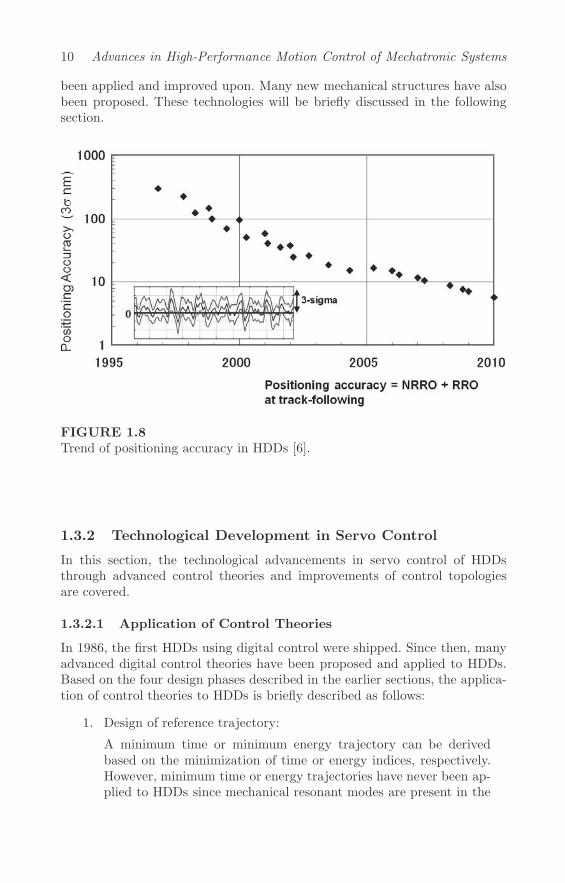
The growth in areal recording density was most rapid from the mid-90sto the early 2000s, where its compound annual growth rate was 100%. Thismeans that the data storage capacity of the shipped HDDs was doubled everyyear. This rapid growth has placed the HDDs in a distinguished position inthe data storage market. The trend of positioning accuracy comprising of bothRepeatable Run-Out (RRO) and Non-Repeatable Run-Out (NRRO) is shownin Figure 1.8 [6]. In order to meet such a rapid increase of areal density, thesynergistic combination of mechanical, electrical, and control design requiredto achieve the desired positioning accuracy has been very challenging. Fromthe control design aspect, it should be noted that many control theories have
10 Advances in High-Performance Motion Control of Mechatronic Systems
been applied and improved upon. Many new mechanical structures have alsobeen proposed. These technologies will be briefly discussed in the followingsection.
FIGURE 1.8Trend of positioning accuracy in HDDs [6].
1.3.2 Technological Development in Servo Control
In this section, the technological advancements in servo control of HDDsthrough advanced control theories and improvements of control topologiesare covered.
1.3.2.1 Application of Control Theories
In 1986, the first HDDs using digital control were shipped. Since then, manyadvanced digital control theories have been proposed and applied to HDDs.Based on the four design phases described in the earlier sections, the applica-tion of control theories to HDDs is briefly described as follows:
1. Design of reference trajectory:
A minimum time or minimum energy trajectory can be derivedbased on the minimization of time or energy indices, respectively.However, minimum time or energy trajectories have never been ap-plied to HDDs since mechanical resonant modes are present in the

Introduction to High-Performance Motion Control of Mechatronic Systems 11
actual servomechanism. In the late 80s, a minimum jerk trajectorywas proposed to reduce residual vibrations in [7]. The input-shapingdesign is a more active approach where a specific resonant frequencyis removed from the designed trajectory [8]. Since the early 2000s,the FSC theory has been applied to HDD servo control. The FSCtheory is a comprehensive approach for trajectory design and re-sults in less excitation of the mechanical resonant modes [9]. Thisdesign method is described in detail in Chapter 2.
2. Design of controllers to track the reference trajectory:
This servo control design is one of the major areas in control theory,and many methods have been proposed. The PTOS [10] was pro-posed in the mid-80s and is one of the most popular methods appliedto HDDs. For the PTOS, power amplifier saturation is consideredfor fast access control in the track-seeking mode, and a smoothtransfer to the linear feedback loop for precise-positioning controlin the track-following mode is provided. The design of the feedfor-ward controller in TDOF control has always been an issue since therealization of the inverse dynamics of the plant model is difficult inmany cases. With the ZPETC proposed in the late 80s [11], TDOFcontrol has been applied to HDDs since the 90s. Model-followingcontrol [12], sliding mode control, N -delay multi-rate feedforwardcontrol [13], and deadbeat control are some other methods whichhave been proposed for HDDs. The PTC [14] proposed around 2000is an excellent design that makes use of multi-rate sampling.
3. Design of transient or settling controller to minimize the trackingerror caused by various unmodeled dynamics or unpredicted para-metric variations in the plants:
This phase is meant for overcoming settling issues in actual HDDproducts. The IVC has been applied to the Mode Switching Control(MSC) structure in HDDs since the early 90s [15]. The details ofthe IVC scheme are described in Chapter 3.
4. Design of controllers to suppress external disturbances to ensurethat the controlled object remains on its target position:
This phase is another very important area in control theory withmany methods proposed in the literature. From the perspective ofrobust stability, Linear Quadratic Gaussian (LQG)/Loop TransferRecovery (LTR) [16], H∞ [17], and H2 control were proposed in theearly 90s. For this design phase, one of the major issues in HDDs isthe handling of the complicated mechanical resonant modes undera given sampling frequency for stabilization of the control system.Phase-stable control design has been applied to HDDs since theearly 2000s, where even the phase information of the mechanicalresonant modes was utilized for stabilization with high servo band-

12 Advances in High-Performance Motion Control of Mechatronic Systems
width [18]. As the mechanical resonant modes are located at bothwithin and above the Nyquist frequency, a comprehensive designand analysis approach has been proposed in [19]. A detailed descrip-tion of this approach is available in Chapter 4. Dual-stage actuationand multi-sensing servo systems have also been proposed since theearly 90s (see Chapter 1.3.2.2). In terms of improving the distur-bance rejection capabilities, the disturbance observer [20], AFC forthe cancellation of external vibrations [21], as well as repetitivecontrol [22] and learning control [23] for the reduction of RRO havebeen proposed since the late 80s.
1.3.2.2 Improvement of Control Structure
For the head-positioning system in HDDs, the magnetic R/W head is usedas the sensor and the VCM is used as the actuator. The distance betweenthe sensor and the actuator is of several centimeters, and all the mechanicaldynamics exist between them. As this structure makes control systems designdifficult, dual-stage actuation has been proposed since the early 90s [24]. Thethree main types of dual-stage actuators are the suspension-driven based,slider-driven based [25], and head-element-driven based [26]. Currently, thesuspension-driven based dual-stage actuators have been implemented in com-mercial HDDs. The MEMS-based slider-driven type and head-element-driventype actuators have been studied for many years and are not commerciallyavailable yet.
On the other hand, an additional sensor can be placed on the arm orsuspension so that a state-feedback loop can be realized. This so-called multi-sensing systems concept has been proposed since the late 90s [27], and isa fairly standard practice in control engineering. From the control systemsperspective, both dual-stage actuation and multi-sensing servo systems areequally difficult to implement. However, both methods have the additionaladvantage of extending the servo bandwidth, and will be described in detailin Chapter 5.
In addition, interested readers are referred to [28]–[32] and the referencestherein for a better understanding of the history of HDD servo control fromvarious perspectives.

Bibliography
[1] T. Yamaguchi, M. Hirata, and C. K. Pang (eds.), High-Speed PrecisionMotion Control, CRC Press, Taylor and Francis Group, Boca Raton, FL,USA, 2011.
[2] C. W. de Silva,Mechatronics: An Integrated Approach, CRC Press, Taylorand Francis Group, Boca Raton, FL, USA, 2004.
[3] S. Ashley, “Getting a Hold on Mechatronics,” Mechanical Engineering,Vol. 119, No. 5, pp. 60–63, May 1997.
[4] R. Wood and H. Takano, “Prospects for Magnetic Recording Over theNext 10 Years,” in Digests of the 2006 IEEE INTERMAG Conference,CA-01, pp. 98, San Diego, CA, USA, May 8–12, 2006.
[5] Y. Shiroishi, K. Fukuda, I. Tagawa, H. Iwasaki, S. Takenoiri, H. Tanaka,H. Mutoh, and N. Yoshikawa, “Future Options for HDD Storage,” IEEETransactions on Magnetics, Vol. 45, No. 10, pp. 3816–3822, October 2009.
[6] T. Yamaguchi and T. Atsumi, “Keynote: HDD Servo ControlTechnologies–What We Have Done and Where We Should Go,” in Pro-ceedings of the 17th IFAC World Congress, MoA21.1, pp. 821–826, Seoul,Korea, July 6–11, 2008.
[7] E. Cooper, “Minimizing Power Dissipation in a Disk File Actuator,”IEEE Transactions on Magnetics, Vol. 24, No. 3, pp. 2081–2091, May1988.
[8] N. Singer and W. Seering, “Preshaping Command Inputs to Reduce Sys-tem Vibration,” Journal of Dynamic Systems, Measurement, and Con-trol, Vol. 112, No. 1, pp. 76–82, March 1990.
[9] M. Hirata, T. Hasegawa, and K. Nonami, “Seek Control of Hard DiskDrives Based on Final-State Control Taking Account of the FrequencyComponents and the Magnitude of Control Input,” in Proceedings ofthe 7th International Workshop on Advanced Motion Control, pp. 40–45,Maribor, Slovenia, July 3–5, 2002.
[10] M. Workman, Adaptive Proximate Time-Optimal Servomechanism,Ph.D. Dissertation, Stanford University, 1987.
13

14 Advances in High-Performance Motion Control of Mechatronic Systems
[11] M. Tomizuka, “Zero Phase Error Tracking Algorithm for Digital Con-trol,” Journal of Dynamic Systems, Measurement and Control, Vol. 109,No. 1, pp. 65–68, March 1987.
[12] M. Iwashiro, M. Yatsu, and H. Suzuki, “Time Optimal Track-to-TrackSeek Control by Model Following Deadbeat Control,” IEEE Transactionson Magnetics, Vol. 35, No. 2, pp. 904–909, March 1999.
[13] S. Takakura, “Design of the Tracking System using N -Delay Two-Degrees-of-Freedom Control and its Application to Hard Disk Drives,”IEEJ Transactions on Industry Applications, Vol. 119, No. 5, pp. 728–734, 1999 (in Japanese).
[14] H. Fujimoto, Y. Hori, T. Yamaguchi, and S. Nakagawa, “Proposal ofPerfect Tracking and Perfect Disturbance Rejection Control by MultirateSampling and Applications to Hard Disk Drive Control,” in Proceedingsof the 38th IEEE Conference on Decision and Control, FrP11, pp. 5277–5282, Phoenix, AZ, USA, December 7–10, 1999.
[15] T. Yamaguchi, S. Shishida, H. Hirai, K. Tsuneta, and M. Sato, “Improve-ment of Servo Robustness for Digital Sector Servo System,” in Digests ofthe 1992 IEEE INTERMAG Conference, GA-12, pp. 332, April 13–16,1992.
[16] S. Weerasooriya and D. T. Phan, “Discrete-Time LQG/LTR Design andModeling of a Disk Drive Actuator Tracking Servo System,” IEEE Trans-actions on Industrial Electronics, Vol. 42, No. 3, pp. 240–247, June 1995.
[17] M. Hirata, K. Liu, T. Mita, and T. Yamaguchi, “Head Positioning Controlof a Hard Disk Drive Using H∞ Theory,” in Proceedings of the 31st IEEEConference on Decision and Control, TP13, pp. 2460–2461, Tucson, AZ,USA, December 16–18, 1992.
[18] T. Atsumi, T. Arisaka, T. Shimizu, and H. Masuda, “Head-PositioningControl Using Resonant Modes in Hard Disk Drives,” IEEE/ASMETransaction on Mechatronics, Vol. 10, No. 4, pp. 378–384, August 2005.
[19] T. Atsumi, “Disturbance Suppression beyond Nyquist Frequency in HardDisk Drives,” in Proceedings of the 17th IFAC World Congress, pp. 827–832, Seoul, Korea, July 6–11, 2008.
[20] M. T. White, M. Tomizuka, and C. Smith, “Rejection of Disk Drive Vi-bration and Shock Disturbances with a Disturbance Observer,” in Pro-ceedings of the American Control Conference, pp. 4127–4131, San Diego,CA, USA, June 2–4, 1999.
[21] M. T. White and M. Tomizuka, “Increased Disturbance Rejection in Mag-netic Disk Drives by Acceleration Feedforward Control,” in Proceedingsof the 13th IFAC World Congress, pp. 489–494, San Francisco, CA, USA,June 30–July 5, 1996.

Bibliography 15
[22] K. Chew and M. Tomizuka, “Digital Control of Repetitive Errors in DiskDrive Systems,” IEEE Control Systems Magazine, Vol. 10, No. 1, pp.16–19, January 1990.
[23] Y. Chen, K. L. Moore, J. Yu, and T. Zhang, “Iterative Learning Con-trol and Repetitive Control in Hard Disk Drive Industry–A Tutorial,” inProceedings of the 45th Conference on Decision and Control, WeTT3.1,pp. 2338–2351, San Diego, CA, USA, December 13–15, 2006.
[24] K. Mori, T. Munemoto, H. Otsuki, Y. Yamaguchi, and K. Akagi, “ADual-Stage Magnetic Disk Drive Actuator Using a Piezoelectric Devicefor High Track Density,” IEEE Transactions on Magnetics, Vol. 27, No.6, pp. 5298–5302, November 1991.
[25] T. Hirano, L. Fan, T. Semba, W. Y. Lee, J. Hong, S. Pattanaik, P.Webb, W. Juan, and S. Chan, “High-Bandwidth HDD Tracking Servoby a Moving-Slider Microactuator,” IEEE Transactions on Magnetics,Vol. 35, No. 5, pp. 3670–3672, September 1999.
[26] H. Toshiyoshi, M. Mita, and T. Fujita, “A MEMS Piggyback Actuatorfor Hard Disk Drives,” IEEE Journal of Microelectromechanical Systems,Vol. 11, No. 6, pp. 648–654, December 2002.
[27] F. Huang, W. Imaino, T. Semba, and F. Lee, “Rotary Actuator Dynamicswith Active Damping,” in Proceedings of the 11th Annual Symposium onInformation Storage and Processing System, Session 8, Santa Clara, CA,June 21–23, 2000.
[28] D. Abramovitch and G. Franklin, “A Brief History of Disk Drive Con-trol,” IEEE Control System Magazine, Vol. 22, No. 3, pp. 28–42, June2002.
[29] W. Messner and R. Ehrlich, “A Tutorial on Controls for Disk Drives,” inProceedings of the American Control Conference, pp. 408–420, Arlington,VA, USA, June 25–27, 2001.
[30] T. Yamaguchi, “Review Paper: Modelling and Control of a Disk FileHead-Positioning System,” Proceedings of the Institution of MechanicalEngineers, Part I: Journal of Systems and Control Engineering, Vol. 215,No. 6, pp. 549–568, September 2001.
[31] A. Al Mamun, G. Guo, and C. Bi, Hard Disk Drive Mechatronics andControl, CRC Press, Taylor and Francis Group, Boca Raton, FL, USA,2006.
[32] T. Yamaguchi, “Guest Editorial Special Issue: ‘Servo Control for DataStorage and Precision Systems,’ from 17th IFAC World Congress 2008,”Mechatronics, Vol. 20, No. 1, pp. 1–5, February 2010.


2
Fast Motion Control Using TDOF ControlStructure and Optimal Feedforward Input
M. Hirata
Utsunomiya University
CONTENTS
2.1 TDOF Control Structure . . . . . . . . . . . . . . . . . . . . . . . . . . . . . . . . . . . . . . . . 182.1.1 One-Degree-Of-Freedom Control System . . . . . . . . . . . . . . . . 182.1.2 Two-Degrees-Of-Freedom Control System . . . . . . . . . . . . . . 192.1.3 Implementation of Feedforward Input by TDOF
Control Structure . . . . . . . . . . . . . . . . . . . . . . . . . . . . . . . . . . . . . . . . 222.2 Optimum Feedforward Input Design . . . . . . . . . . . . . . . . . . . . . . . . . . . . 23
2.2.1 Minimum Time Control . . . . . . . . . . . . . . . . . . . . . . . . . . . . . . . . . 232.2.2 Minimum Jerk Input . . . . . . . . . . . . . . . . . . . . . . . . . . . . . . . . . . . . 242.2.3 Digital Implementation of Minimum Jerk Input . . . . . . . . 272.2.4 Sampled-Data Polynomial Input . . . . . . . . . . . . . . . . . . . . . . . . 28
2.3 Final-State Control . . . . . . . . . . . . . . . . . . . . . . . . . . . . . . . . . . . . . . . . . . . . . . 332.3.1 Problem Formulation . . . . . . . . . . . . . . . . . . . . . . . . . . . . . . . . . . . . 332.3.2 Minimum Jerk Input Design by FSC . . . . . . . . . . . . . . . . . . . 342.3.3 Vibration Minimized Input Design by FSC . . . . . . . . . . . . . 352.3.4 Final-State Control with Constraints . . . . . . . . . . . . . . . . . . . 38
2.4 Industrial Application: Hard Disk Drives . . . . . . . . . . . . . . . . . . . . . . . . 392.4.1 HDD Benchmark Problem and the Plant Model . . . . . . . . 392.4.2 FSC and FFSC Inputs Design . . . . . . . . . . . . . . . . . . . . . . . . . . . 42
2.5 Industrial Application: Galvano Scanner I . . . . . . . . . . . . . . . . . . . . . . . 482.5.1 Plant Model . . . . . . . . . . . . . . . . . . . . . . . . . . . . . . . . . . . . . . . . . . . . . 482.5.2 FSC and FFSC Inputs Design . . . . . . . . . . . . . . . . . . . . . . . . . . . 492.5.3 Simulation Results . . . . . . . . . . . . . . . . . . . . . . . . . . . . . . . . . . . . . . . 532.5.4 Experimental Results . . . . . . . . . . . . . . . . . . . . . . . . . . . . . . . . . . . . 54
2.6 Industrial Application: Galvano Scanner II . . . . . . . . . . . . . . . . . . . . . . 582.6.1 Voltage Saturation in Current Amplifier . . . . . . . . . . . . . . . . 582.6.2 FSC Design Considering Voltage Saturation in Current
Amplifier . . . . . . . . . . . . . . . . . . . . . . . . . . . . . . . . . . . . . . . . . . . . . . . . . 592.6.3 Application to Galvano Scanner Control Problem . . . . . . 61
17
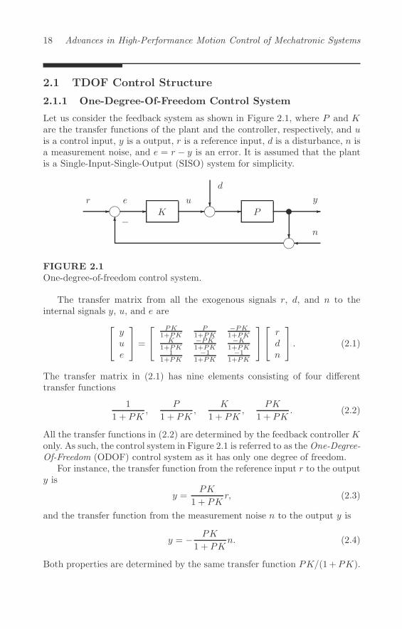
18 Advances in High-Performance Motion Control of Mechatronic Systems
2.1 TDOF Control Structure
2.1.1 One-Degree-Of-Freedom Control System
Let us consider the feedback system as shown in Figure 2.1, where P and Kare the transfer functions of the plant and the controller, respectively, and uis a control input, y is a output, r is a reference input, d is a disturbance, n isa measurement noise, and e = r − y is an error. It is assumed that the plantis a Single-Input-Single-Output (SISO) system for simplicity.
K � P�� � � � �
�
� �r e
−
u y
d
���n
FIGURE 2.1One-degree-of-freedom control system.
The transfer matrix from all the exogenous signals r, d, and n to theinternal signals y, u, and e are
⎡⎣yue
⎤⎦ =
⎡⎣
PK1+PK
P1+PK
−PK1+PK
K1+PK
−PK1+PK
−K1+PK
11+PK
−11+PK
−11+PK
⎤⎦⎡⎣rdn
⎤⎦ . (2.1)
The transfer matrix in (2.1) has nine elements consisting of four differenttransfer functions
1
1 + PK,
P
1 + PK,
K
1 + PK,
PK
1 + PK. (2.2)
All the transfer functions in (2.2) are determined by the feedback controllerKonly. As such, the control system in Figure 2.1 is referred to as the One-Degree-Of-Freedom (ODOF) control system as it has only one degree of freedom.
For instance, the transfer function from the reference input r to the outputy is
y =PK
1 + PKr, (2.3)
and the transfer function from the measurement noise n to the output y is
y = − PK
1 + PKn. (2.4)
Both properties are determined by the same transfer function PK/(1+PK).

TDOF Control Structure and Optimal Feedforward Input 19
P�u
�K�
�y
r�
FIGURE 2.2General formulation of two-degrees-of-freedom control system.
K� P
�
�
� �y
r
u��
�−� �
FIGURE 2.3ODOF controller in TDOF controller structure.
As such, it is impossible to reduce the influence of the measurement noisewhile the reference input response is kept unchanged. The design of the ODOFcontroller hence requires severe trade-off among various control properties.
2.1.2 Two-Degrees-Of-Freedom Control System
As for the reference input, a filter F can be introduced1 such as
r = F r. (2.5)
Using the filter F , the reference input response can be improved while theother feedback properties are kept intact. In this way, control performancecan be determined by not only the feedback controller K but also by the filterF . This control system is referred to as the Two-Degrees-Of-Freedom (TDOF)control system since it has two degrees of design freedom.
The general formulation of the TDOF control system is shown in Fig-ure 2.2, where the TDOF controller uses the reference input r and the outputy separately, while the ODOF controller uses the error e = r − y only. TheODOF control system can be regarded as a special case of the TDOF controlsystem as shown in Figure 2.3.
There are many types of the TDOF control system, and the typical TDOFconfigurations of control systems are shown in Figure 2.4. It should be noted
1Other than the reference input such as disturbance and measurement noise, the intro-duction of the filter is physically impossible.

20 Advances in High-Performance Motion Control of Mechatronic Systems
that the control system of Figure 2.4(a) has a TDOF control structure thoughit has no feedforward controller.
Among these TDOF control systems, the design of Figure 2.4(c) is rela-tively easy and straightforward because the reference response property andthe other feedback properties can be determined separately. The TDOF con-trol system of Figure 2.4(c) is referred to as the Model-Matching Two-Degrees-Of-Freedom (MMTDOF) control system.
In the MMTDOF control system, M is referred to as the reference model,and the feedforward controller GFF is determined so that the transfer functionfrom r to y becomes M . This can be achieved by setting
GFF =M
P, (2.6)
as
y =
[PK
1 + PKM +
P
1 + PKGFF
]r (2.7)
=
[PK
1 + PKM +
P
1 + PK
M
P
]r
=
[PK
1 + PK+
1
1 + PK
]M r
= M r. (2.8)
The reference model M must be selected so that M and M/P are stable andproper. If P has unstable zeros, M must have the same zeros to cancel inM/P .
Equation (2.8) shows that the reference response property can be deter-mined solely by M independently of the feedback properties in the ideal case,i.e., the plant has no uncertainties. This is the distinctive feature of the TDOFcontrol system.
If the plant has uncertainties, the reference response property may bedegraded. Let us show the effect of the plant uncertainties when the plant hasa multiplicative uncertainty as
P = (1 +Δ)P.
The transfer function from r to y is
y =
[PK
1 + PKM +
(1 +Δ)P
1 + PK
M
P
]r
=
[PK
1 + PK+
(1 +Δ)
1 + PK
]M r
=
[PK
1 + PK+
1
1 + PK+
Δ
1 + PK
]M r
=
[1 + Δ
1
1 + PK
]M r. (2.9)
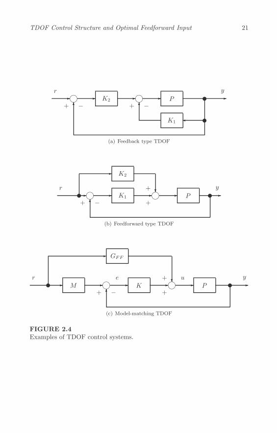
TDOF Control Structure and Optimal Feedforward Input 21
K2 P
K1
�� �
�
�� �
�
�
�
yr
−�
�
+ + −
(a) Feedback type TDOF
P�K1
K2
�� � � � ��
�
�
��yr
−+
+
+
(b) Feedforward type TDOF
P�K�M� � � � � �
�
GFF�
��r ue
�y
−+ +
+
(c) Model-matching TDOF
FIGURE 2.4Examples of TDOF control systems.

22 Advances in High-Performance Motion Control of Mechatronic Systems
In (2.9), the effect of the multiplicative uncertainty Δ appears as
Δ1
1 + PK,
where 1/(1 + PK) is the sensitivity function of the actual feedback controlsystem. As such, the robustness of the reference response can be improvedby designing the sensitivity function of the control system to be small at thefrequencies where the plant has uncertainties.
2.1.3 Implementation of Feedforward Input by TDOF Con-trol Structure
As shown in the previous section, the reference response can be determinedby selecting the reference model M in the MMTDOF control system. Forexample, if P = 1/s2, the reference model can be selected as
M =ω2n
s2 + 2ζωns+ ω2n
.
The design parameters ζ and ωn are adjusted so that the reference model Mhas a good step response. However, it is unclear whether the selected valuesare optimal or not. Moreover, it is difficult to take into account the inputsaturation and/or the constraints on some state variables of the plant usingthis framework.
An optimal feedforward input obtained by minimizing a cost function sub-jected to constraints may solve this problem. This optimal feedforward inputplays an important role to achieve high-performance motion control. Suchfeedforward inputs must be implemented with a feedback controller becausefeedforward control has no robustness against disturbances and plant uncer-tainties. The feedforward input uFF can be implemented by the TDOF controlstructure as shown in Figure 2.5. In Figure 2.5, the transfer function from uFFto y is P if P = P . When P �= P or disturbances exist, the feedback controllerK minimizes the error between the actual output y(t) and the output ym(t)of the nominal model.
P�K��P� � � � � ��
�
�
−+
+
+
uFF
ym yue
FIGURE 2.5Implementation of feedforward input by the TDOF control structure.

TDOF Control Structure and Optimal Feedforward Input 23
P e−τds�K��Pe−τds� � � � � ��
�
�
−+
+
+
uFF
ym yue
FIGURE 2.6Implementation of feedforward input when plant has input delay.
When the plant has an input delay τd and becomes P e−τds, the TDOFcontrol structure of Figure 2.6 can be used instead of Figure 2.5. When P = P ,the transfer function from uFF to y becomes Pe−τds. This means that thefeedforward input uFF can be designed to the nominal plant P without inputdelay, and the input delay is taken into account when uFF is implemented tothe TDOF control system.
2.2 Optimum Feedforward Input Design
2.2.1 Minimum Time Control
The use of the optimal feedforward input is very effective to achieve fast andprecise motion control. Theoretically, the minimum time control can achievealso minimum time positioning [1].
The minimum time control input can be obtained by minimizing the costfunction
J(T ) =
∫ T
0
1 dt,
subject to the boundary conditions
y(0) = 0, y(T ) = r, y(0) = 0, y(T ) = 0,
and the input limitation|u(t)| ≤ umax.
When the plant is a rigid-body system
y =1
s2u,
the optimal solution is
u(t) =
⎧⎨⎩
+umax (0 ≤ t < Topt/2)−umax (Topt/2 ≤ t < Topt)0 (t < 0, Topt ≤ t)
, (2.10)
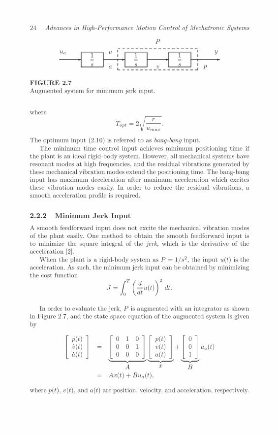
24 Advances in High-Performance Motion Control of Mechatronic Systems
1
s
1
s�� �
P
1
s�
ua yu
a v p
FIGURE 2.7Augmented system for minimum jerk input.
where
Topt = 2
√r
umax.
The optimum input (2.10) is referred to as bang-bang input.
The minimum time control input achieves minimum positioning time ifthe plant is an ideal rigid-body system. However, all mechanical systems haveresonant modes at high frequencies, and the residual vibrations generated bythese mechanical vibration modes extend the positioning time. The bang-banginput has maximum deceleration after maximum acceleration which excitesthese vibration modes easily. In order to reduce the residual vibrations, asmooth acceleration profile is required.
2.2.2 Minimum Jerk Input
A smooth feedforward input does not excite the mechanical vibration modesof the plant easily. One method to obtain the smooth feedforward input isto minimize the square integral of the jerk, which is the derivative of theacceleration [2].
When the plant is a rigid-body system as P = 1/s2, the input u(t) is theacceleration. As such, the minimum jerk input can be obtained by minimizingthe cost function
J =
∫ T
0
(d
dtu(t)
)2
dt.
In order to evaluate the jerk, P is augmented with an integrator as shownin Figure 2.7, and the state-space equation of the augmented system is givenby
⎡⎣p(t)v(t)a(t)
⎤⎦ =
⎡⎣
0 1 00 0 10 0 0
⎤⎦
︸ ︷︷ ︸A
⎡⎣p(t)v(t)a(t)
⎤⎦
︸ ︷︷ ︸x
+
⎡⎣
001
⎤⎦
︸ ︷︷ ︸B
ua(t)
= Ax(t) +Bua(t),
where p(t), v(t), and a(t) are position, velocity, and acceleration, respectively.

TDOF Control Structure and Optimal Feedforward Input 25
With this augmented system, the cost function becomes a simple form of
J =
∫ T
0
(d
dtu(t)
)2
dt =
∫ T
0
u2a(t) dt.
At the initial time t = 0 and the final time t = T , the velocity and theacceleration should be zero. The position of the actuator moves from the originto the target position r. The boundary conditions are given by
x(0) =
⎡⎣
000
⎤⎦ , x(T ) =
⎡⎣r00
⎤⎦ .
In order to obtain the optimal solution, the Hamiltonian H is defined as
H = u2a + λT (Ax +Bua).
The costate equation
−λ =∂H
∂x= ATλ
becomes
−⎡⎣λ1λ2λ3
⎤⎦ =
⎡⎣
0 0 01 0 00 1 0
⎤⎦⎡⎣λ1λ2λ3
⎤⎦ . (2.11)
From the stationary condition
∂H
∂ua= 2ua +BTλ = 0,
we have
ua = −1
2BTλ = −1
2λ3. (2.12)
From (2.11), we have
λ1 = c′1λ2 = −c′1t+ c′2
λ3 =c′12t2 − c′2t+ c′3. (2.13)
From (2.12) and (2.13), we have
ua(t) = −1
2
{c′12t2 − c′2t+ c′3
}.
Since
a(t) =
∫ t
0
ua(t)dt,

26 Advances in High-Performance Motion Control of Mechatronic Systems
and a(0) = 0, the acceleration can be described as
a(t) = c1
(t
T
)3
+ c2
(t
T
)2
+ c3
(t
T
).
From v(0) = 0 and y(0) = 0, we can obtain
v(t) = T
{c14
(t
T
)4
+c23
(t
T
)3
+c32
(t
T
)2},
p(t) = T 2
{c120
(t
T
)5
+c212
(t
T
)4
+c36
(t
T
)3}.
With u(T ) = 0, v(T ) = 0, and p(T ) = r, the following simultaneous equationmust hold ⎡
⎣1 1 13 4 63 5 10
⎤⎦
⎡⎣c1c2c3
⎤⎦ =
⎡⎣
001
⎤⎦ 60
T 2r,
and the unique solution is
⎡⎣c1c2c3
⎤⎦ =
⎡⎣
10 −5 2−12 7 −3
3 −2 1
⎤⎦⎡⎣
001
⎤⎦ 60
T 2r =
⎡⎣
2−31
⎤⎦ 60
T 2r.
Finally, we have the minimum jerk input and the trajectories of p(t), v(t),a(t) as
p(t) = 60r
{1
10
(t
T
)5
− 1
4
(t
T
)4
+1
6
(t
T
)3},
v(t) =30r
T
{(t
T
)4
− 2
(t
T
)3
+
(t
T
)2},
a(t) =60r
T 2
{2
(t
T
)3
− 3
(t
T
)2
+
(t
T
)}.
The minimum jerk input umjc(t) for the rigid-body system P = 1/s2
becomes
umjc(t) = a(t) =60r
T 2
{2
(t
T
)3
− 3
(t
T
)2
+
(t
T
)}(2.14)
=60r
T 2tn(2tn − 1)(tn − 1), (2.15)
where tn = t/T . The time response of the minimum jerk input and the tra-jectories v(t) and p(t) are shown in Figure 2.8.

TDOF Control Structure and Optimal Feedforward Input 27
0 0.1 0.2 0.3 0.4 0.5 0.6 0.7 0.8 0.9 1−5
0
5
Time [s]
a(t)
0 0.1 0.2 0.3 0.4 0.5 0.6 0.7 0.8 0.9 10
1
2
Time [s]
v(t)
0 0.1 0.2 0.3 0.4 0.5 0.6 0.7 0.8 0.9 10
0.5
1
Time [s]
p(t)
FIGURE 2.8Minimum jerk input.
2.2.3 Digital Implementation of Minimum Jerk Input
Recently, positioning control algorithms in mechatronic products are imple-mented by microprocessor in most cases. As such, the minimum jerk inputumjc(t) (which is a continuous-time signal) must be implemented by using asampler-and-hold as shown in Figure 2.9. In this figure, ZOH is the Zero-OrderHold and τ is a sampling period. In this case, the output y(t) of the plantmay not go to the target position if the sampling period cannot be chosenarbitrarily small enough.
ZOH1
s2� �
u(t) y(t)���τ
umjc(t) umjc(τk)�� �
FIGURE 2.9Digital implementation of umjc(t).
As an example, the output response y(t) in Figure 2.9 is calculated fordifferent sampling periods. The final time T and the target position r in(2.14) are assumed to be T = 1 and r = 1. The outputs y(t) are shownin Figure 2.10 when τ = 10 ms and τ = 100 ms. Figure 2.10 shows that the

28 Advances in High-Performance Motion Control of Mechatronic Systems
0 0.1 0.2 0.3 0.4 0.5 0.6 0.7 0.8 0.9 1−6
−4
−2
0
2
4
6
Time [s]
Inpu
t
0 0.1 0.2 0.3 0.4 0.5 0.6 0.7 0.8 0.9 10
0.2
0.4
0.6
0.8
1
Time [s]
Out
put
τ = 10msτ = 100ms
FIGURE 2.10Minimum jerk control for different sampling periods.
positioning error at t = T becomes large if the sampling period is not smallenough as τ = 100 ms.
An approach to avoid the positioning error at the final time t = T is toobtain the feedforward input by taking into account the effects of the ZOH.The details of this approach will be presented in the next section.
2.2.4 Sampled-Data Polynomial Input
A feedforward input generated by a polynomial taking account of the effectof the ZOH is referred to as the sampled-data polynomial input [3].
Similarly, the plant P (s) is assumed to be a rigid-body system as
P (s) =1
s2.
The state-space representation of P (s) can be given as
[p(t)v(t)
]=
[0 10 0
] [p(t)v(t)
]+
[01
]u(t), (2.16)
where p(t) is the position, v(t) is the velocity, and u(t) is the input.

TDOF Control Structure and Optimal Feedforward Input 29
It is assumed that the input u(t) is generated by a discrete-time signalu[n] (n = 0, 1, 2, . . .) through the ZOH as
u(τn+ θ) = u[n], θ ∈ [0, τ).
As such, (2.16) can be discretized as[p[n+ 1]v[n+ 1]
]=
[1 τ0 1
] [p[n]v[n]
]+
[12τ
2
τ
]u[n], (2.17)
where p[n] = p(τn) and v[n] = v(τn).When the initial values of p[0], v[0], and u[0] are set as zero, it is straight-
forward to show that v[n] and p[n] are given by
v[n] =
⎧⎪⎨⎪⎩
0 (n ≤ 1)
τn−1∑i=1
u[i] (2 ≤ n), (2.18)
p[n] =
⎧⎪⎨⎪⎩
0 (n ≤ 1)
1
2τ2
n−1∑i=1
[{2(n− i)− 1}u[i]] (2 ≤ n). (2.19)
Similar to the minimum jerk input, the discrete-time feedforward inputu[n] is assumed to be a polynomial of order three as
u[n] = An3 +Bn2 + Cn+D, (2.20)
where the coefficient A, B, C, and D must satisfy the initial conditions
u[0] = 0, v[0] = 0, p[0] = 0,
and the final conditions
u[N ] = 0, v[N ] = 0, p[N ] = r,
where N is a final step.From u[0] = 0, we have
D = 0.
From u[N ] = 0, we have
u[N ] = N3A+N2B +NC = 0. (2.21)
From v[N ] = 0, we have
v[N ] = τ
N−1∑i=1
u[i]
= τN−1∑i=1
(Ai3 +Bi2 + Ci)
= XAA+XBB +XCC = 0, (2.22)

30 Advances in High-Performance Motion Control of Mechatronic Systems
where
XA = τ
N−1∑i=1
i3 =τ
4N2(N − 1)2,
XB = τ
N−1∑i=1
i2 =τ
6N(N − 1)(2N − 1),
XC = τ
N−1∑i=1
i =τ
2N(N − 1).
From p[N ] = r, we have
p[N ] =1
2τ2
N−1∑i=1
[{2(N − i)− 1}u[i]]
= YAA+ YBB + YCC = r, (2.23)
where
YA =τ2
2
N−1∑i=1
{(2N − 1)i3 − 2i4
}=
τ2
120N(N − 1)(2N − 1)(3N2 − 3N + 4),
YB =τ2
2
N−1∑i=1
{(2N − 1)i2 − 2i3
}=τ2
12N(N − 1)(N2 −N + 1),
YC =τ2
2
N−1∑i=1
{(2N − 1)i− 2i2
}=τ2
12N(2N − 1)(N − 1).
By solving (2.21), (2.22), and (2.23) simultaneously, we have
A =120r
τ21
N(N2 − 1)(N2 − 4),
B = −180r
τ21
(N2 − 1)(N2 − 4),
C =60r
τ2N
(N2 − 1)(N2 − 4),
and the sampled-data polynomial of (2.20) becomes
u[n] =60r
τ2n(n−N)(2n−N)
N(N2 − 1)(N2 − 4). (2.24)
In order to compare the minimum jerk input (2.15) and the sampled-datapolynomial (2.24), the normalized step nn = n/N and the final time T = τNare introduced. Equation (2.24) becomes
u[n] =60r
T 2nn(2nn − 1)(nn − 1)g, (2.25)
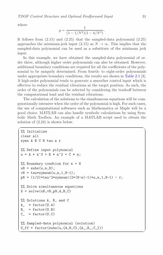
TDOF Control Structure and Optimal Feedforward Input 31
where
g =1
(1− 1/N2)(1− 4/N4).
It follows from (2.15) and (2.25) that the sampled-data polynomial (2.25)approaches the minimum-jerk input (2.15) as N → ∞. This implies that thesampled-data polynomial can be used as a substitute of the minimum jerkinput.
In this example, we have obtained the sampled-data polynomial of or-der three, although higher order polynomials can also be obtained. However,additional boundary conditions are required for all the coefficients of the poly-nomial to be uniquely determined. From fourth- to eight-order polynomialsunder appropriate boundary conditions, the results are shown in Table 2.1 [3].A high-order polynomial tends to generate a smoother control input which iseffective to reduce the residual vibrations at the target position. As such, theorder of the polynomials can be selected by considering the tradeoff betweenthe computational load and the residual vibrations.
The calculation of the solutions to the simultaneous equations will be com-putationally intensive when the order of the polynomial is high. For such cases,the use of computational softwares such as Mathematica or Maple will be agood choice. MATLAB can also handle symbolic calculations by using Sym-bolic Math Toolbox. An example of a MATLAB script used to obtain thesolution of (2.24) is shown below.�
�
�
%% Initialize
clear all
syms A B C N tau n r
%% Define input polynomial
u = A * n^3 + B * n^2 + C * n;
%% Boundary condtion for n = N
uN = subs(u,n,N);
vN = tau*symsum(u,n,1,N-1);
pN = (1/2)*tau^2*symsum((2*(N-n)-1)*u,n,1,N-1) - r;
%% Solve simultaneous equations
S = solve(uN,vN,pN,A,B,C)
%% Solutions A, B, and C
A_ = factor(S.A)
B_ = factor(S.B)
C_ = factor(S.C)
%% Sampled-data polynomial (solution)
U_ff = factor(subs(u,{A,B,C},{A_,B_,C_}))

32 Advances in High-Performance Motion Control of Mechatronic Systems
TABLE 2.1Acceleration Sampled-Data Polynomials
Order Boundary conditions and polynomial u[n]
Fourthp[0] = v[0] = u[0] = 0, p[N ] = r,v[N ] = u[N ] = d
dnu[N ] = 0
u[n] =−60n(n−N)2(5nN − 2(1 +N2))r
(N − 2)(N − 1)N(N + 1)(N + 2)(1 +N2)τ2
Fifthp[0] = v[0] = u[0] = d
dnu[0] = 0, p[N ] = r,v[N ] = u[N ] = d
dnu[N ] = 0
u[n] =−420n2(n−N)2(2n−N)r
(N − 2)(N − 1)N(N + 1)(N + 2)(5 +N2))τ2
Sixthp[0] = v[0] = u[0] = d
dnu[0] = 0, p[N ] = r,
v[N ] = u[N ] = ddnu[N ] = d2
dn2u[N ] = 0
u[n] =840n2(n−N)3(−10 + (7n− 3N)N(1 +N2))r
N(N2 − 4)(N2 − 1)(N2 + 5)(10 + 3(N2 +N4))τ2
Seventhp[0] = v[0] = u[0] = d
dnu[0] =d2
dn2u[0] = 0, p[N ] = r,
v[N ] = u[N ] = ddnu[N ] = d2
dn2u[N ] = 0
u[n] =2520n3(n−N)3(2n−N)r
(N − 2)(N − 1)N(N + 1)(N + 2)(42 + 5N2 +N4)τ2
Eighthp[0] = v[0] = u[0] = d
dnu[0] =d2
dn2u[0] = 0, p[N ] = r,
v[N ] = u[N ] = ddnu[N ] = d2
dn2u[N ] = d3
dn3u[N ] = 0
u[n] =−1260n3(n−N)4
(N − 2)(N − 1)N(N + 1)(N + 2)(3 +N2)
× (−84 + 30nN − 4N2 + 9nN3 − 4N4 + 9nN5 − 4N6)r
(7− 2N2 +N4)(42 + 5N2 +N4)τ2
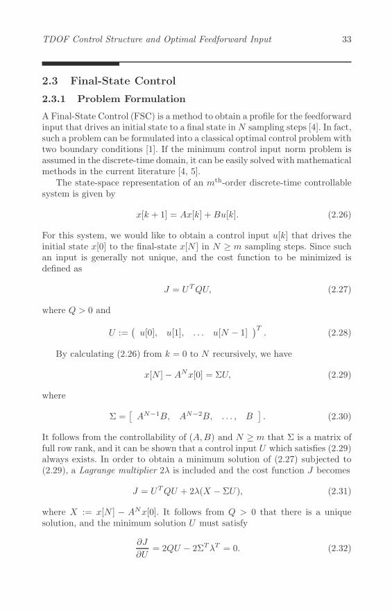
TDOF Control Structure and Optimal Feedforward Input 33
2.3 Final-State Control
2.3.1 Problem Formulation
A Final-State Control (FSC) is a method to obtain a profile for the feedforwardinput that drives an initial state to a final state inN sampling steps [4]. In fact,such a problem can be formulated into a classical optimal control problem withtwo boundary conditions [1]. If the minimum control input norm problem isassumed in the discrete-time domain, it can be easily solved with mathematicalmethods in the current literature [4, 5].
The state-space representation of an mth-order discrete-time controllablesystem is given by
x[k + 1] = Ax[k] +Bu[k]. (2.26)
For this system, we would like to obtain a control input u[k] that drives theinitial state x[0] to the final-state x[N ] in N ≥ m sampling steps. Since suchan input is generally not unique, and the cost function to be minimized isdefined as
J = UTQU, (2.27)
where Q > 0 and
U :=(u[0], u[1], . . . u[N − 1]
)T. (2.28)
By calculating (2.26) from k = 0 to N recursively, we have
x[N ]−ANx[0] = ΣU, (2.29)
where
Σ =[AN−1B, AN−2B, . . . , B
]. (2.30)
It follows from the controllability of (A,B) and N ≥ m that Σ is a matrix offull row rank, and it can be shown that a control input U which satisfies (2.29)always exists. In order to obtain a minimum solution of (2.27) subjected to(2.29), a Lagrange multiplier 2λ is included and the cost function J becomes
J = UTQU + 2λ(X − ΣU), (2.31)
where X := x[N ] − ANx[0]. It follows from Q > 0 that there is a uniquesolution, and the minimum solution U must satisfy
∂J
∂U= 2QU − 2ΣTλT = 0. (2.32)

34 Advances in High-Performance Motion Control of Mechatronic Systems
Since Q > 0 and Q−1 exists, we have
U = Q−1ΣTλT . (2.33)
Furthermore, it follows from X−ΣU = 0 and (2.33) that X−ΣQ−1ΣTλT = 0is satisfied. Since Σ is a matrix of full row rank by the controllability of (A,B),|ΣQ−1ΣT | �= 0 is also satisfied. As such, we have
λT = (ΣQ−1ΣT )−1X. (2.34)
Finally, it follows from (2.33) and (2.34) that [5]
U = Q−1ΣT (ΣQ−1ΣT )−1(x[N ] −ANx[0]). (2.35)
The optimal feedforward input U can now be easily obtained using simplealgebra for given x[0], x[N ], Q, and N .
Pc(s) � ���� �ZOH1
z − 1
uc(t)���
u[k] y[k]
P [z]
y(t)uc[k]
τ
Pd[z]
FIGURE 2.11Augmented system with a discrete-time integrator.
2.3.2 Minimum Jerk Input Design by FSC
The minimum jerk input in discrete-time domain can be easily solved byusing the proposed FSC method. Similar to the minimum jerk input design incontinuous-time domain as shown in Section 2.2.2, an augmented system witha discrete-time integrator 1/(z − 1) as shown in Figure 2.11 is considered. InFigure 2.11, Pc(s) is a continuous-time plant whose input is acceleration (orforce or the same dimension of those) and Pd[z] is a discretized plant of Pc(s).
Since the input of the augmented system corresponds to jerk, the minimumjerk input can be obtained by minimizing the cost function
J =
∞∑k=0
uT [k]u[k]. (2.36)
The state-space representation of Pc(s) which is of mth-order is given by
xc(t) = Acxc(t) +Bcuc(t), y(t) = Ccxc(t), (2.37)

TDOF Control Structure and Optimal Feedforward Input 35
and the state-space representation of the discrete-time model Pd[z] with ZOHis given by
xd[k + 1] = Adxd[k] +Bduc[k], y[k] = Cdxd[k], (2.38)
where
Ad = eAcτ , Bd =
∫ τ
0
eActBcdt, Cd = Cc,
xd[k] = xc(kτ), y[k] = y(kτ),
and τ is the sampling period. Since the ZOH is used, we have
uc(kτ + θ) = uc[k], θ ∈ [0, τ). (2.39)
The state-space representation of the augmented system is thus given by
x[k + 1] = Ax[k] +Bu[k], y[k] = Cx[k], (2.40)
where x[k] := [xTd [k], uTc [k]]
T and
A =
[Ad Bd0 1
], B =
[01
], C =
[Cd 0
]. (2.41)
In this case, both (Ac, Bc) and (Ad, Bd) are assumed to be controllable.Now, a smooth input is obtained by applying the FSC method to the aug-
mented system in (2.40) via minimizing the cost function in (2.36) subjectedto both initial and final state constraints. It should be noted that the initialand final states of the augmented system have to be given by
x[0] =
[xd[0]uc[0]
]= 0(m+1)×1, x[N ] =
[xd[N ]uc[N ]
]=
[xd[N ]0
], (2.42)
so that the actual input uc satisfies uc[0] = 0 and uc[N ] = 0. The feedfor-ward input obtained by this method is referred to as the FSC input and thetrajectory generated by the FSC input is referred to as the FSC trajectory.
2.3.3 Vibration Minimized Input Design by FSC
A smooth input is desired to reduce the residual vibrations after positioning.However, such an input may extend beyond the total positioning time. In orderto achieve both high-speed positioning and vibration suppression, we considerminimizing the spectrum of the control input at the frequencies where resonantmodes of the plant exist [5].
The Fourier transform Uc(ω) of uc(t) is defined as
Uc(ω) =
∫ Nτ
0
uc(t)e−jωtdt, (2.43)

36 Advances in High-Performance Motion Control of Mechatronic Systems
and its gain |Uc(ω)| is minimized at the desired frequency points ωi(i =1, . . . , ). For this purpose, the following cost function is introduced as
Jw =
N−1∑k=0
u2[k] +
�∑i=1
qi|Uc(ωi)|2. (2.44)
The first term of the right-hand side of (2.44) evaluates the smoothness ofthe control input, and the second term evaluates the frequency componentsof the control input. By choosing ωi to cover the frequencies of the resonantmodes of the plant, the frequency components around these frequencies arereduced. The weighting parameter qi is selected to be a positive real number,and a larger qi achieves a larger reduction in frequency components.
In order to obtain the closed-form of U which minimizes (2.44), the state-space representation of the discrete-time integrator is given by
1
z − 1= {1, 1, 1, 0} =: {Aw, Bw, Cw, 0}. (2.45)
Assuming uc[0] = 0, the actual control input uc[k] can be described by
Uc = ΩwU, (2.46)
where
Uc =[uc[0], . . . , uc[N − 1]
]T, (2.47)
and
Ωw =
⎡⎢⎢⎢⎢⎢⎢⎢⎢⎣
0 0 . . . . . . 0
CwBw 0. . .
...
CwAwBw CwBw. . .
. . ....
.... . .
. . . 0 0
CwAN−2w Bw . . . CwAwBw CwBw 0
⎤⎥⎥⎥⎥⎥⎥⎥⎥⎦. (2.48)
Since uc(t) is the output of the ZOH, we have
uc(t) =
N−1∑i=0
Pi(t)uc[k], (2.49)
where
Pi(t) :=
{1, iτ ≤ t < (i+ 1)τ0, t < iτ or t ≥ (i+ 1)τ
. (2.50)
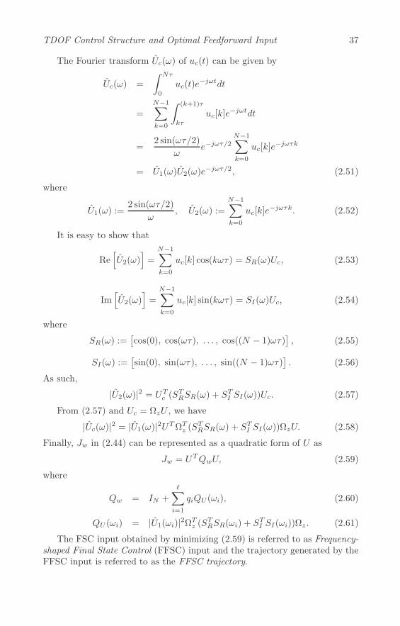
TDOF Control Structure and Optimal Feedforward Input 37
The Fourier transform Uc(ω) of uc(t) can be given by
Uc(ω) =
∫ Nτ
0
uc(t)e−jωtdt
=
N−1∑k=0
∫ (k+1)τ
kτ
uc[k]e−jωtdt
=2 sin(ωτ/2)
ωe−jωτ/2
N−1∑k=0
uc[k]e−jωτk
= U1(ω)U2(ω)e−jωτ/2, (2.51)
where
U1(ω) :=2 sin(ωτ/2)
ω, U2(ω) :=
N−1∑k=0
uc[k]e−jωτk. (2.52)
It is easy to show that
Re[U2(ω)
]=
N−1∑k=0
uc[k] cos(kωτ) = SR(ω)Uc, (2.53)
Im[U2(ω)
]=
N−1∑k=0
uc[k] sin(kωτ) = SI(ω)Uc, (2.54)
where
SR(ω) :=[cos(0), cos(ωτ), . . . , cos((N − 1)ωτ)
], (2.55)
SI(ω) :=[sin(0), sin(ωτ), . . . , sin((N − 1)ωτ)
]. (2.56)
As such,
|U2(ω)|2 = UTc (STRSR(ω) + STI SI(ω))Uc. (2.57)
From (2.57) and Uc = ΩzU , we have
|Uc(ω)|2 = |U1(ω)|2UTΩTz (STRSR(ω) + STI SI(ω))ΩzU. (2.58)
Finally, Jw in (2.44) can be represented as a quadratic form of U as
Jw = UTQwU, (2.59)
where
Qw = IN +�∑i=1
qiQU (ωi), (2.60)
QU (ωi) = |U1(ωi)|2ΩTz (STRSR(ωi) + STI SI(ωi))Ωz . (2.61)
The FSC input obtained by minimizing (2.59) is referred to as Frequency-shaped Final State Control (FFSC) input and the trajectory generated by theFFSC input is referred to as the FFSC trajectory.

38 Advances in High-Performance Motion Control of Mechatronic Systems
2.3.4 Final-State Control with Constraints
In actual control problems, the maximum absolute value of the control inputis limited due to saturation. Moreover, the minimum or maximum value ofvelocity, acceleration, and current may also be limited. In this case, the feed-forward input must be designed so as to satisfy these constraints. In order toincorporate the constraints into the FSC design, the constraint variable z[k]is introduced as
z[k] = Czx[k] +Dzu[k], (2.62)
and the control input u[k] which minimizes (2.27) is obtained subjected to
|z[k]| < zmax (k = 0, . . . , N − 1), (2.63)
for a given zmax.
This problem can be formulated as a Quadratic Programming (QP) prob-lem [6]. The QP is a problem to obtain a solution U ∈ RN minimizing thecost function
J = UTQU, (2.64)
with Q > 0 and subjected to one or more constraints of the form
AEQU = bEQ (equality constraint), (2.65)
AINEQU ≤ bINEQ (inequality constraint), (2.66)
where AEQ and AINEQ are arbitrary matrices, and bEQ and bINEQ are arbi-trary vectors. The notation AINEQU ≤ bINEQ means that every entry of thevector AINEQU is less than or equal to the corresponding entry of the vectorbINEQ.
In the FSC method, the equality constraint in (2.29) corresponds to (2.65),and the cost function (2.27) corresponds to (2.64). In addition, constraints onthe state variables and/or the input of the plant can easily be handled byutilizing the inequality constraints in (2.66).
Without loss of generality, z[k] is assumed to be a scalar variable, andz[0], . . . , z[N − 1] are calculated as
⎧⎪⎪⎪⎨⎪⎪⎪⎩
z[0] = Czx[0] +Dzu[0]z[1] = CzAx[0] + CzBu[0] +Dzu[1]
...z[N − 1] = CzA
N−1x[0] + · · ·+Dzu[N − 1]
. (2.67)
Equation (2.67) can be represented collectively in a matrix form as
Z = Φzx[0] + ΩzU, (2.68)

TDOF Control Structure and Optimal Feedforward Input 39
where
Z =[z[0], · · · , z[N − 1]
]T, (2.69)
Φz =
⎡⎢⎢⎢⎣
CzCzA...
CzAN−1
⎤⎥⎥⎥⎦ , (2.70)
Ωz =
⎡⎢⎢⎢⎢⎢⎢⎢⎢⎣
0 0 . . . . . . 0
CzB 0. . .
...
CzAB CzB. . .
. . ....
.... . .
. . . 0 0
CzAN−2B . . . CzAB CzB 0
⎤⎥⎥⎥⎥⎥⎥⎥⎥⎦. (2.71)
As such, the constraint in (2.63) can be represented as an inequality as
[Ωz
−Ωz
]U ≤
[Zmax − Φzx[0]Zmax +Φzx[0]
], (2.72)
where Zmax = zmax[1, . . . , 1]T . Since (2.72) corresponds to (2.66), the FSC
and FFSC problems with constraints can be reformulated as QP problems.
2.4 Industrial Application: Hard Disk Drives
The FSC and FFSC inputs are designed for the plant of the Hard Disk Drive(HDD) Benchmark Problem [7], and the control performance is evaluated bysimulations.
2.4.1 HDD Benchmark Problem and the Plant Model
Various control methods have been proposed for HDD servo problems so far.However, it is difficult to compare and evaluate these control methods fairlybecause they have been developed for a specific control objective and on differ-ent HDDs. As such, the demand for the benchmark problem of HDD controlhas been tremendously increased.
To realize these purposes, the “Investigation R&D Committee for NextGeneration Servo Control Technology for Mass-Storage System,” the Chairbeing Dr. Takashi Yamaguchi, at the Institute of Electrical Engineers of Japan(IEEJ) set up a working group to develop the HDD Benchmark Problemtogether. In September 2005, the working group released Version 1 of theHDD Benchmark Problem, in which plant parameters are optimized for the

40 Advances in High-Performance Motion Control of Mechatronic Systems
TABLE 2.2Plant Parameters
i fi [Hz] ζi Ai1 0 0 1.02 3000 0.01 −0.013 4100 0.03 −1.04 5000 0.01 0.35 7000 0.01 −1.06 12300 0.005 1.07 16400 0.005 −1.0
TABLE 2.3Parameter Variations
Variable min (%) max (%)f2 −2 % +1 %f3 −5 % +2.5 %f4,5,6,7 −2 % +0.5 %A2,4 −200 % +0 %A3 −0 % +20 %ζ5,6,7 −50 % +100 %
track-following controller design. In the following year, the plant model wasupdated to reflect more realistic properties of actual HDDs, and Version 2 ofthe HDD Benchmark Problem was released. Finally in 2010, the plant modelsin Versions 1 and 2 were unified in the latest version or Version 3 of theHDD Benchmark Problem, where both models can now be used by selectingthe corresponding parameter files [8, 9]. In this section, the parameter set inVersion 2 of the HDD Benchmark Problem is used.
The transfer function of the plant model is defined as
Pf (s) = Kp
(N∑i=1
Ais2 + 2ζiωis+ ω2
i
)e−sTd , (2.73)
where ωi = 2πfi, Kp = 3.93× 10⁹, and Td = 1 × 10⁻⁵s. The control input isthe acceleration [m/s2] of the voice coil motor and the measurement output isthe head position [track]. The parameters Ai, ζi, and fi of the resonant modesare shown in Table 2.2, and the frequency response of the nominal model isshown in Figure 2.12. The HDD Benchmark Problem also includes a model ofparameter variation of the mechanical resonant mode. The upper and lowerbounds of the parameters are shown in Table 2.3, and the frequency responsesof the perturbed models are shown in Figure 2.13. The change in loop gain of±10% is also assumed.
In the HDD Benchmark Problem for track-seeking, the following assump-tions are made:
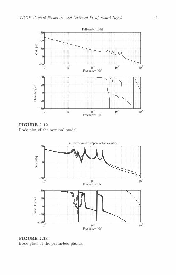
TDOF Control Structure and Optimal Feedforward Input 41
101 102 103 104 105−50
0
50
100
150G
ain
[dB
]
Frequency [Hz]
Full−order model
101 102 103 104 105−180
−90
0
90
180
Phas
e [d
egre
e]
Frequency [Hz]
FIGURE 2.12Bode plot of the nominal model.
103 104 105−50
0
50
Gai
n [d
B]
Frequency [Hz]
Full−order model w/ parametric variation
103 104 105−180
−90
0
90
180
Phas
e [d
egre
e]
Frequency [Hz]
FIGURE 2.13Bode plots of the perturbed plants.

42 Advances in High-Performance Motion Control of Mechatronic Systems
1. no disturbances are taken into account;2. the magnitude of the control input is not limited;3. two seek distances of one track and ten tracks are considered; and4. the seeking time is defined as the time in which the head position
settles within ±0.1 of the track width at the target track for all thenominal and perturbed models.
The main object of the track-seeking control problem is to design a track-seeking control system which achieves the shortest seeking time for both oneand ten track-seeks. The controller parameters can be optimized for both oneand ten track-seeks as long as the same control method is used.
This section focuses on the design of the feedforward input that reducesthe residual vibrations. As such, a feedback controller is not used. In theHDD Benchmark Problem, a plant gain change of ±5% is included. For oursimulations, the gain change is not considered because the gain change cannotbe compensated for without the feedback controller.
2.4.2 FSC and FFSC Inputs Design
Design 1
In Design 1, a minimum jerk input for a rigid-body mode model was obtainedusing the FSC method. The step number N was determined by trial and errorso that the maximum seeking times for all the plant model are minimized. Asa result, N = 12 achieved the minimum seeking time for one track-seek. Thecorresponding time response and the spectrum of the obtained minimum jerkinput are shown in Figure 2.14.
Track-seeking simulations were then carried out, and the time responsesand the spectra of the head positions for all the plant models are shown inFigure 2.15. The worst-case seek time was 0.333 ms.
As for ten track-seek, N = 26 achieves the minimum seeking time. Thecorresponding time response and the spectrum of the obtained minimum jerkinput is shown in Figure 2.16. The time responses and the spectra of the headposition for all the plant models are shown in Figure 2.17. The worst-case seektime was 0.879 ms.
In both one and ten track-seek, it was difficult to further decrease the seektime since the head position varies beyond ±10% of the track width due toresidual vibrations.
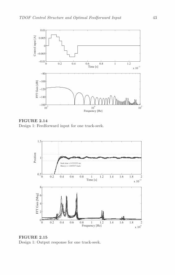
TDOF Control Structure and Optimal Feedforward Input 43
0 0.2 0.4 0.6 0.8 1 1.2x 10⁻³
−0.01
−0.005
0
0.005
0.01
Time [s]
Con
trol i
nput
[A]
103 104 105−160
−140
−120
−100
−80
Frequency [Hz]
FFT
Gai
n [d
B]
FIGURE 2.14Design 1: Feedforward input for one track-seek.
0 0.2 0.4 0.6 0.8 1 1.2 1.4 1.6 1.8 2x 10⁻³
0.5
1
1.5
Time [s]
Posi
tion
Seek time = 0.333333 msMax(y) = 1.045537 track
0 0.2 0.4 0.6 0.8 1 1.2 1.4 1.6 1.8 2x 10⁴
0
2
4
6
8
Frequency [Hz]
FFT
Gai
n [M
ag]
FIGURE 2.15Design 1: Output response for one track-seek.

44 Advances in High-Performance Motion Control of Mechatronic Systems
0 0.5 1 1.5 2 2.5x 10⁻³
−0.02
−0.01
0
0.01
0.02
Time [s]
Con
trol i
nput
[A]
103 104 105−160
−140
−120
−100
−80
Frequency [Hz]
FFT
Gai
n [d
B]
FIGURE 2.16Design 1: Feedforward input for ten track-seek.
0 0.2 0.4 0.6 0.8 1 1.2 1.4 1.6 1.8 2x 10⁻³
9.5
10
10.5
Time [s]
Posi
tion
Seek time = 0.878788 msMax(y) = 10.078912 track
0 0.2 0.4 0.6 0.8 1 1.2 1.4 1.6 1.8 2x 10⁴
0
2
4
6
8
Frequency [Hz]
FFT
Gai
n [M
ag]
FIGURE 2.17Design 1: Output response for ten track-seek.

TDOF Control Structure and Optimal Feedforward Input 45
Design 2
In Design 2, the FFSC method was applied to minimize the residual vibra-tions. In the FFSC method, the selections of the frequencies ωi = 2πfi andthe weights qi in (2.44) are very important to reduce the residual vibrationswithout extending the seek time.
In the HDD Benchmark Problem, the lower- and upper-bound of the fre-quency changes of the resonant modes are defined for each vibration mode asshown in Table 2.3. As such, the cost function is modified so that the designparameters can easily be tuned for each vibration mode separately as [7]
Jw =1
N
N−1∑k=0
u2[k] +7∑i=3
�i∑j=1
qi|Uc(2πfij)|2, (2.74)
where
fij = f�i +fui − f�ii − 1
j, (j = 1 · · · i). (2.75)
The plant in the HDD Benchmark Problem has six vibration modes at3 kHz, 4.1 kHz, 5 kHz, 7 kHz, 12.3 kHz, and 16.4 kHz. The FFSC input wasdesigned so that the spectra at 4.1 kHz, 5 kHz, 7 kHz, and 12.3 kHz are wellreduced for one track-seek as these modes cause large residual vibrations. Theparameters of (2.74) and (2.75) are shown in Table 2.4. Note that i = 60 forall i.
TABLE 2.4Design Parameters for Design 2
i f�i (Hz) fhi (Hz) qi (1 track) qi (10 tracks)3 3895 4305 5× 10⁹ 5× 10⁹
4 4900 5050 2× 10⁸ 2× 10⁸
5 6860 7070 1× 10¹⁰ 5× 10¹⁰
6 12054 12423 2× 10⁹ 1× 10⁹
7 16072 16564 0 1× 10⁸
On the other hand, for ten track-seek, the FFSC input was designed so thatthe spectra at 4.1 kHz, 5 kHz, 7 kHz, 12.3 kHz, and 16.4 kHz are well reduced.The design parameters are also shown in Table 2.4. The seek stepN was chosenso that the worst-case seek time is minimized for all the plant models. N = 10for one track-seek and N = 17 for ten track-seek were determined. The timeresponses and the spectra of the FFSC inputs are shown in Figure 2.18 andFigure 2.20. The time responses and the spectra of the head position are shownin Figure 2.19 and Figure 2.21. The seek time was 0.280 ms for one track-seekand 0.538 ms for ten track-seek, resulting in 16% and 39% improvements ofseek time, respectively.

46 Advances in High-Performance Motion Control of Mechatronic Systems
0 0.2 0.4 0.6 0.8 1x 10⁻³
−0.02
−0.01
0
0.01
0.02
Time [s]
Con
trol i
nput
[A]
103 104 105−160
−140
−120
−100
−80
Frequency [Hz]
FFT
Gai
n [d
B]
FIGURE 2.18Design 2: Feedforward input for one track-seek.
0 0.2 0.4 0.6 0.8 1 1.2 1.4 1.6 1.8 2x 10⁻³
0.5
1
1.5
Time [s]
Posi
tion
Seek time = 0.280303 msMax(y) = 1.081692 track
0 0.2 0.4 0.6 0.8 1 1.2 1.4 1.6 1.8 2x 10⁴
0
2
4
6
8
Frequency [Hz]
FFT
Gai
n [M
ag]
FIGURE 2.19Design 2: Output response for one track-seek.
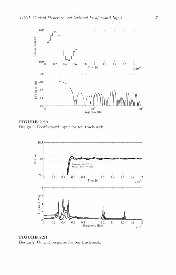
TDOF Control Structure and Optimal Feedforward Input 47
0 0.2 0.4 0.6 0.8 1 1.2 1.4 1.6 1.8x 10⁻³
−0.05
0
0.05
Time [s]
Con
trol i
nput
[A]
103 104 105−160
−140
−120
−100
−80
Frequency [Hz]
FFT
Gai
n [d
B]
FIGURE 2.20Design 2: Feedforward input for ten track-seek.
0 0.2 0.4 0.6 0.8 1 1.2 1.4 1.6 1.8 2x 10⁻³
9.5
10
10.5
Time [s]
Posi
tion
Seek time = 0.537879 msMax(y) = 10.075286 track
0 0.2 0.4 0.6 0.8 1 1.2 1.4 1.6 1.8 2x 10⁴
0
2
4
6
8
Frequency [Hz]
FFT
Gai
n [M
ag]
FIGURE 2.21Design 2: Output response for ten track-seek.

48 Advances in High-Performance Motion Control of Mechatronic Systems
2.5 Industrial Application: Galvano Scanner I
The laser-drilling machine for printed wiring boards is required to processsmaller diameter holes with higher precision and throughput. The galvanoscanner is a key component in the laser processing machine, and it has amirror to control the direction of the laser beam. The angle of the mirrormust be controlled as quickly and precisely as possible.
In this section, the FSC and FFSC inputs are designed for the galvano scan-ner, and the obtained feedforward inputs are implemented using the TDOFcontrol structure. The effectiveness of the proposed method is verified withsimulations and experiments [10].
2.5.1 Plant Model
The control system of the galvano scanner is shown in Figure 2.22.
FIGURE 2.22Control system of galvano scanner.
In Figure 2.22, i is a motor current, iref is a reference to the motor current,and y is a motor angle. The measured frequency response from iref to y isshown in Figure 2.23 by the solid line. Note that the unit [Hz/unit] is anormalized frequency where the frequency of the first resonant mode is unity.As shown in Figure 2.23, the plant has two large resonant modes at highfrequencies.
To fit the measured frequency response, the transfer function of the galvanoscanner is modeled as a system having a rigid-body mode and two vibrationmodes with an input delay as
P (s) = Pmech(s)e−τds,
where Pmech is defined as
Pmech(s) = Pn(s) + P1(s) + P2(s), (2.76)
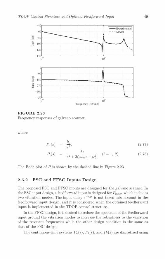
TDOF Control Structure and Optimal Feedforward Input 49
10−1 100−140
−120
−100
−80
−60
−40
Gai
n [d
B]
ExperimentalModel
10−1 100
0
−90
−180
−270
−360
−450
Frequency [Hz/unit]
Phas
e [d
eg]
FIGURE 2.23Frequency responses of galvano scanner.
where
Pn(s) =k0s2, (2.77)
Pi(s) =ki
s2 + 2ζiωnis+ ω2ni
(i = 1, 2). (2.78)
The Bode plot of P is shown by the dashed line in Figure 2.23.
2.5.2 FSC and FFSC Inputs Design
The proposed FSC and FFSC inputs are designed for the galvano scanner. Inthe FSC input design, a feedforward input is designed for Pmech which includestwo vibration modes. The input delay e−τds is not taken into account in thefeedforward input design, and it is considered when the obtained feedforwardinput is implemented in the TDOF control structure.
In the FFSC design, it is desired to reduce the spectrum of the feedforwardinput around the vibration modes to increase the robustness to the variationof the resonant frequencies while the other design condition is the same asthat of the FSC design.
The continuous-time systems Pn(s), P1(s), and P2(s) are discretized using

50 Advances in High-Performance Motion Control of Mechatronic Systems
the ZOH method, and their state-space representations are given as
Pn[z] :
{xn[k + 1] = Anxn[k] +Bnuc[k]
yn[k] = Cnxn[k], (2.79)
P1[z] :
{x1[k + 1] = A1x1[k] +B1uc[k]
y1[k] = C1x1[k], (2.80)
P2[z] :
{x2[k + 1] = A2x2[k] +B2uc[k]
y2[k] = C2x2[k], (2.81)
where the state vectors are defined as
xn[k] =
[xnpxnv
], x1[k] =
[x1px1v
], x2[k] =
[x2px2v
].
Note that the subscripts p and v of the state variables denote the position andthe velocity of each mode, respectively.
Under these definitions, the discrete-time state-space representation ofPmech is given as
Pmech[z] :
{xd[k + 1] = Adxd[k] +Bduc[k]
y[k] = Cdxd[k], (2.82)
where
Ad =
⎡⎣An 0 00 A1 00 0 A2
⎤⎦ , Bd =
⎡⎣BnB1
B2
⎤⎦ , Cd =
[Cn C1 C2
],
xd[k] =
⎡⎣xn[k]x1[k]x2[k]
⎤⎦ .
To design the FSC input, the augmented system of Figure 2.24 is consid-ered which corresponds to the augmented system of Figure 2.11. The statevector of the augmented system is defined as
x[k] =
[xd[k]uc[k]
],
and the initial and the final states are given as
x[0] =
[xd[0]uc[0]
]=
⎡⎢⎢⎣xn[0]x1[0]x2[0]uc[0]
⎤⎥⎥⎦ =
⎡⎢⎢⎣
0000
⎤⎥⎥⎦ ,
x[N ] =
[xd[N ]uc[N ]
]=
⎡⎢⎢⎣xn[N ]x1[N ]x2[N ]uc[N ]
⎤⎥⎥⎦ =
⎡⎢⎢⎢⎢⎣
[r0
]
000
⎤⎥⎥⎥⎥⎦,

TDOF Control Structure and Optimal Feedforward Input 51
1
z − 1Pmech[z]� � �
u[k] uc[k] y[k]
FIGURE 2.24Augmented system to design the FSC and FFSC inputs for the galvano scan-ner.
where r is the target position. The step number N is determined as N = 79so that the feedforward input does not saturate. The obtained FSC inputand its spectrum are shown in Figure 2.25 and Figure 2.26 by the dashedline, respectively. In Figure 2.25, the unit [s/unit] of the horizontal axis is anormalized time so that the final time is one second and the unit [A/unit]is a unit when the target position is normalized to r = 1. In Figure 2.26,the vertical dashed line of the left-hand side represents the primary resonantfrequency, and that of the right-hand side represents the secondary resonantfrequency. From Figure 2.26, it is confirmed that the spectra at the resonantfrequency are well reduced, and the width of the notch of each frequency isvery narrow.
Next, the FFSC input was obtained by reducing the spectra around theprimary and the secondary resonant modes. The parameter ωi in the costfunction (2.44) is selected to cover the resonant frequency variation of ±6%of the primary and secondary vibration modes as
ωi =
⎧⎪⎨⎪⎩
0.94ωn1 +1.06ωn1 − 0.94ωn1
50× (i − 1), (i = 1, . . . , 50)
0.94ωn2 +1.06ωn2 − 0.94ωn2
50× (i − 51), (i = 51, . . . , 100)
where ωn1 and ωn2 are the resonant frequencies of the primary and secondaryvibration modes, respectively. The weighing parameter qi is selected to be
qi =
{1× 10⁹, (i = 1, . . . , 50)5× 10⁷, (i = 51, . . . , 100)
.
The weight qi for the primary vibration mode is selected to be larger thanthat of the secondary vibration mode because the frequency change of theprimary vibration mode easily increases the residual vibrations as comparedto that of the secondary vibration mode in this system.
The obtained FFSC input and its spectrum are shown in Figure 2.25 andFigure 2.26 by the solid line, respectively. From Figure 2.26, it is confirmedthat the spectrum of the input is well reduced not only at the resonant frequen-cies but also over the frequency interval where the frequency varies. As such,the robustness to the frequency changes of the resonant modes is expected toincrease.
Note that the maximum absolute value of the FFSC input is larger thanthat of the FSC input. The design parameters must be selected so as not toexceed the maximum value of the control input.

52 Advances in High-Performance Motion Control of Mechatronic Systems
0 0.2 0.4 0.6 0.8 1 1.2−2000
−1500
−1000
−500
0
500
1000
1500
2000
Time [s/unit]
FSC
/FFS
C in
put [
A/u
nit]
FFSC inputFSC input
FIGURE 2.25Time responses of FSC and FFSC inputs.
10−1 100−120
−100
−80
−60
−40
−20
0
Frequency [Hz/unit]
Gai
n [d
B]
FFSC inputFSC input
FIGURE 2.26Spectra of FFSC and FSC inputs.

TDOF Control Structure and Optimal Feedforward Input 53
���Pmeche−τds� � � � � ��
�
�
−+
+
+
uFF
ym yuePP
Pmeche−τdsK
FIGURE 2.27MMTDOF control system for galvano scanner control system.
2.5.3 Simulation Results
The robustness to the resonant frequency variation is evaluated by simulations.Since the plant has an input delay e−τds, the MMTDOF control system takinginto account the input delay as explained in Section 2.1.3 was used. The blockdiagram of the MMTDOF control system is shown in Figure 2.27, and thefeedback controller in commercial products was used.
0 0.5 1 1.5 2 2.5 30.996
0.998
1
1.002
1.004
Posi
tion
[rad
/uni
t]
0 0.5 1 1.5 2 2.5 30.996
0.998
1
1.002
1.004
Time [s/unit]
Posi
tion
[rad
/uni
t]
FSC
FFSC
FIGURE 2.28Simulated time responses of output when the frequency of the primary vibra-tion mode is changed from −6% to +6%.
The upper figure in Figure 2.28 shows the output response y of the FSCinput at the target position when the primary resonant mode of the plantwas changed from −6% to +6% at 1% intervals. Note that [rad/unit] is thenormalized unit so that the target position is equal to unity.
54 Advances in High-Performance Motion Control of Mechatronic Systems
The bottom figure of Figure 2.28 shows the output response of the FFSCinput under the same condition to the FSC input simulation. By comparingthe results of the FSC and FFSC inputs, the FFSC input achieves smallerresidual vibrations. The effectiveness of the frequency shaping using the FFSCmethod has been confirmed.
2.5.4 Experimental Results
Experiments were conducted by using the same TDOF control structure asthe simulations. The output response of the FSC input is shown in Figure 2.30by the dashed line. The output converged to the target position with an over-shoot. Since the allowable positioning error of this galvano scanner is ±0.08%of the target position, the positioning time is approximately 1.33 s/unit. Notethat the 1 rad/unit corresponds to several hundreds μrad, and the tolerablepositioning error is the nano-scale.
The output response of the FFSC input is shown by the solid line. Theovershoot and undershoot are larger than the results of the FSC input. Thepositioning time is 1.39 s/unit, which is also slower than the FSC input. Theresidual vibrations of both methods are almost the same. As such, the FSCinput achieves good nominal performance than the FFSC input.
Next, the robustness to the frequency variations of the resonant modesis evaluated. However, it is difficult to change the resonant frequency of theactual system arbitrarily. The resonant frequency of the plant model to designthe FSC and FFSC inputs was changed instead. The FSC and FFSC inputswere designed by changing the primary resonant frequency to +6% of thenominal frequency. The spectra of the obtained FSC and FFSC inputs areshown in Figure 2.29. From Figure 2.29, it can be observed that the frequencywhere the magnitude of the spectrum is reduced around the primary vibrationmode is shifted to the higher frequencies.
The output responses obtained by experiments are shown in Figure 2.31.In Figure 2.31, a large residual vibration is observed in the output response ofthe FSC input and the performance degradation is significant. The positioningtime is also extended from 1.33 s/unit to 1.94 s/unit. The FSC input has poorrobustness to the frequency changes of the vibration modes.
On the other hand, the output of the FFSC input maintains lower residualvibrations as shown in Figure 2.31 by the solid line. The positioning time isextended from 1.39 s/unit to 1.44 s/unit, but the extension is quite smallcompared with that obtained by the FSC input. These results are supportedby the spectrum of the FFSC input as shown in Figure 2.29 by the solidline. The spectrum around the primary resonant mode is still reduced evenif the design frequency of the primary resonant mode is shifted to +6% ofthe nominal frequency. As such, the FFSC input has good robustness to thefrequency change of the resonance modes.
Finally, in order to evaluate the residual vibrations quantitatively, thespectrum of the residual vibration was calculated as shown in Figure 2.32.

TDOF Control Structure and Optimal Feedforward Input 55
Figure 2.32 shows that the peak of the spectrum obtained by the FSC inputaround 1 Hz/unit is drastically reduced by the FFSC input.
10−1 100−120
−100
−80
−60
−40
−20
0
Frequency [Hz/unit]
Gai
n [d
B]
FFSC inputFSC input
FIGURE 2.29Spectra of FSC and FFSC inputs when nominal frequency of primary vibrationmode is perturbed to +6% of the nominal frequency in both FSC and FFSCdesigns.

56 Advances in High-Performance Motion Control of Mechatronic Systems
0 0.5 1 1.5 2 2.5 30.996
0.997
0.998
0.999
1
1.001
1.002
1.003
1.004
Time [s/unit]
Posi
tion
[rad
/uni
t]
FFSC inputFSC input
FIGURE 2.30Experimental time responses of outputs.
0 0.5 1 1.5 2 2.5 30.996
0.997
0.998
0.999
1
1.001
1.002
1.003
1.004
Time [s/unit]
Posi
tion
[rad
/uni
t]
FFSC inputFSC input
FIGURE 2.31Experimental time responses of outputs when nominal frequency of primaryvibration mode is perturbed to +6% of the nominal frequency in both FSCand FFSC designs.
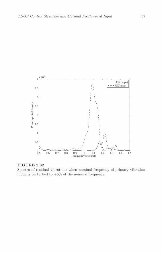
TDOF Control Structure and Optimal Feedforward Input 57
0.5 0.6 0.7 0.8 0.9 1 1.1 1.2 1.3 1.4 1.50
0.5
1
1.5
2
2.5
3
3.5
4x 10⁶
Frequency [Hz/unit]
Pow
er sp
ectra
l den
sity
FFSC inputFSC input
FIGURE 2.32Spectra of residual vibrations when nominal frequency of primary vibrationmode is perturbed to +6% of the nominal frequency.

58 Advances in High-Performance Motion Control of Mechatronic Systems
2.6 Industrial Application: Galvano Scanner II
In order to control the galvano mirror as quickly and precisely as possible, thebandwidth of the current amplifier must be increased. To respond to theserequirements, the maximum voltage of the current amplifier is also increased.However, further increase of the voltage may be difficult to achieve as theheat generated at the current amplifier will be unacceptable. Although a PulseWidth Modulation (PWM) amplifier may resolve the heat problem, it is diffi-cult to achieve the required control accuracy. As such, linear amplifiers are stillused for galvano scanners in order to achieve high-speed and high-precisionpositioning.
In recent years, several studies have examined trajectory design methodsthat constrain control input and/or some state variables [11, 12, 13]. However,few studies have considered the voltage constraint of the current amplifier. Ananti-windup method can be applied when the voltage is saturated, althoughperformance degradation is inevitable. The feedforward input should be de-signed so as not to saturate in advance.
In this section, a FFSC design method that can take into account the volt-age constraint of the current amplifier is introduced [6]. By constraining theapplied voltage to the motor, the power supply voltages of the current am-plifier is lowered. The energy consumption and heat generated by the currentamplifier can also be reduced.
2.6.1 Voltage Saturation in Current Amplifier
In order to explain the FFSC methods considering the voltage constraint of thecurrent amplifier, the control system of Figure 2.33, where a rigid-body system(with no friction) driven by an ideal electromagnetic actuator is considered. Asshown in Figure 2.33, current feedback is realized by analog circuit to achievea higher bandwidth in most cases. In Figure 2.33, Pc(s) is the rigid-bodysystem, Kt is the torque constant, J is the moment of inertia, xp(t) is theposition, xv(t) is the velocity, R is the armature resistance, L is the armatureinductance, Ke is the back electromotive force coefficient, and K(s) is thecurrent feedback controller. It is assumed that the current feedback controllerK(s) is designed so that the actual current i(t) follows the reference currentiref (t) over wide frequency range. The applied voltage VM (t) to the armatureis limited by the power supply voltage Vp. Voltage saturation occurs when theoutput of K(s) exceeds Vp.
If the controllerK(s) of the current amplifier is known, the applied voltageVM (t) can be represented by the state variables of the closed-loop system. Thevoltage constraint problem can then treated by the FSC or FFSC methodswith constraints. However, this may be difficult for the following reasons:
1. The parameters of the current feedback controllerK(s) are required

TDOF Control Structure and Optimal Feedforward Input 59
11
FIGURE 2.33Control system with current amplifier.
1ZOH
11
FIGURE 2.34Augmented system for rigid-body mode model.
in order to design the FSC or FFSC input. As such, the trajectorymust be redesigned when the current amplifier is replaced; and
2. Obtaining information about the current feedback controller K(s)is often difficult in the case of commercially available current am-plifiers.
A method that does not depend on the current feedback controller K(s) isrequired.
2.6.2 FSC Design Considering Voltage Saturation in CurrentAmplifier
Generally, the reference input iref (t) to the current amplifier is followed bythe actual current i(t) with a sufficiently small tracking error because thebandwidth of the current feedback loop is designed to be high. i(t) = iref (t)almost always holds, and the augmented system of Figure 2.34 can be used forFSC and FFSC input design by ignoring the current amplifier and assumingthat the current i(t) is the control input uc(t). In Section 2.5, it has beenshown that the FSC and FFSC inputs designed by using the augmented systemof Figure 2.24 achieve good control performances when the input voltage isnot saturated. If the FSC and FFSC inputs could be designed based on theaugmented system of Figure 2.34 to satisfy the input voltage constraint, thecontrol performances are expected to be satisfactory.
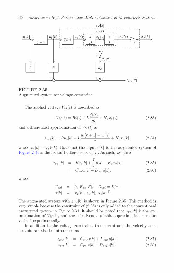
60 Advances in High-Performance Motion Control of Mechatronic Systems
1ZOH
11
FIGURE 2.35Augmented system for voltage constraint.
The applied voltage VM (t) is described as
VM (t) = Ri(t) + Ldi(t)
dt+Kexv(t), (2.83)
and a discretized approximation of VM (t) is
zvol[k] = Ruc[k] + Luc[k + 1]− uc[k]
τ+Kexv[k], (2.84)
where xv[k] = xv(τk). Note that the input u[k] to the augmented system ofFigure 2.34 is the forward difference of uc[k]. As such, we have
zvol[k] = Ruc[k] +L
τu[k] +Kexv[k] (2.85)
= Cvolx[k] +Dvolu[k], (2.86)
where
Cvol = [0, Ke, R], Dvol = L/τ,
x[k] = [xp[k], xv[k], uc[k]]T .
The augmented system with zvol[k] is shown in Figure 2.35. This method isvery simple because the constraint of (2.86) is only added to the conventionalaugmented system in Figure 2.34. It should be noted that zvol[k] is the ap-proximation of VM (t), and the effectiveness of this approximation must beverified experimentally.
In addition to the voltage constraint, the current and the velocity con-straints can also be introduced as
zcur[k] = Ccurx[k] +Dcuru[k], (2.87)
zvel[k] = Cvelx[k] +Dvelu[k], (2.88)

TDOF Control Structure and Optimal Feedforward Input 61
where
Ccur = [0, 0, 1], Dcur = 0,
Cvel = [0, 1, 0], Dvel = 0.
When zvol[k], zcur[k], and zvel[k] are constrained simultaneously, z[k] in (2.62)and zmax in (2.63) are selected to be
z[k] = [zvol[k], zcur[k], zvel[k]]T
zmax = [zmaxvol , zmaxcur , z
maxvel ]T ,
where the superscript max denotes the maximum value of each constraint statevariable.
2.6.3 Application to Galvano Scanner Control Problem
The FFSC input is designed for the model Pmech of (2.76). As Pmech consistsof the rigid-body mode and two vibration modes, the constraint variables ofvoltage, current, and velocity are redefined as zvol, zcur, and zvel, respectively,by using the state variables of Pmech and transformation T as
zvol[k] = CvolTx[k] +Dvolu[k],
zcur[k] = CcurTx[k] +Dcuru[k],
zvel[k] = CvelTx[k] +Dvelu[k],
where
T =
⎡⎣
1 0 1 0 1 0 00 1 0 1 0 1 00 0 0 0 0 0 1
⎤⎦ , x[k] =
[xd[k]uc[k]
],
and xd[k] is the state vector of Pmech[z] defined in (2.82).In the control system of the galvano scanner, the current is limited to less
than 12 A due to the limitation of the current amplifier. The velocity is limitedto less than 5 m/s due to the limitation of the bandwidth of the encoder. Asfor the limitation of the applied voltage to the motor, three types of conditionsare provided, i.e., no constraint, less than 72 V, and less than 36 V.
The trajectory of a 1 mm step control was designed under these constraints.The 1 mm step is commonly used to evaluate the control performance of thegalvano scanner. The step number N = 73 is selected such that the residualvibrations are sufficiently small when the voltage is not saturated.
To design the FFSC input, ωi and qi in (2.44) were set to the same valuesas used in Section 2.5, where the voltage constraint was not considered. Thetime responses of the voltage, current, and velocity of the obtained trajectoriesare shown in Figure 2.36. Figure 2.36 shows that the trajectories satisfy theconstraints.
In the experiments, the obtained FFSC inputs were applied to the galvano

62 Advances in High-Performance Motion Control of Mechatronic Systems
scanner by using the MMTDOF control system as shown in Figure 2.27 takinginto account the input delay. First, the control performance of the FFSC inputwhich does not introduce the voltage constraint is evaluated. Figure 2.37 showsthe position responses for three different power supply voltages of Vp = 162 V,76 V, and 72 V. Since the maximum value of VM was 146 V and the voltagedrop of the current amplifier was 16 V, the voltage of the current amplifiermust have been saturated, except for the case in which Vp = 162 V. FromFigure 2.37, there is no difference between the position responses of Vp = 162 Vand 76 V. However, the settling performance of the result of Vp = 72 V isdegraded. Since the required positioning accuracy of the galvano scanner is±3μm in this case, the positioning time of Vp = 72 V is extended.
Next, two different FFSC inputs were designed with the constraints ofzmaxvol = 72 V and 36 V. Since there is a voltage drop of 16 V in the currentamplifier, the power supply voltage can be reduced to Vp = 88 V and 52 Vfor the FFSC inputs designed under the constraints of zmaxvol =72 V and 36 V,respectively. Figure 2.38 shows the experimental results for the case in whichthe solid, dashed, and dotted lines show the results without the voltage con-straint (Vp = 162 V), with the voltage constraint of Vp = 88 V (zmaxvol = 72 V),and that of Vp = 52 V (zmaxvol = 36 V), respectively. Figure 2.38 shows thata significant performance degradation cannot be seen even for the result forthe case where Vp = 52 V. As such, the FFSC input design with the volt-age constraint is very effective in reducing the power supply voltage withoutperformance degradation.
Since all the energy consumption in the current amplifier is transferredinto heat losses, the heat is evaluated by the amount of energy consumption.The energy consumption in the current amplifier in the ideal condition can becalculated by
Pamp =1
Nτ
∫ Nτ
0
|i(t)|(Vp − |VM (t)|)dt, (2.89)
where VM (t) is the voltage of the motor, and Vp is the supply voltage.In order to compare the energy consumption, the FFSC inputs of the
0.1 mm step and 10 mm step were also obtained. The step numbers N for0.1 mm and 10 mm step controls were selected to be 37 and 351, respectively.The other parameters were selected to be the same as that of 1 mm stepcontrol.
The results are shown in Figure 2.39. Note that the result without inputconstraint is indicated as the constraint voltage of 146 V because the maximumvoltage was 146 V. When (2.89) was calculated, the voltage Vp was selectedto be 52 V, 88 V, and 162 V corresponding to the voltage constraint of 36 V,72 V, and no constraint, respectively, as the current amplifier has an internalvoltage drop of 16 V. As shown in Figure 2.39, the energy consumption isdrastically reduced by lowering the constraint voltage.
It should be noted that the energy consumption for a 10 mm step is lowerthan that for 0.1 mm and 1 mm steps. As Pamp in (2.89) is the average powerconsumption per unit of time and the reference trajectory of 10 mm step has

TDOF Control Structure and Optimal Feedforward Input 63
a constant velocity interval where the current is zero, Pamp for the 10 mm isreduced.

64 Advances in High-Performance Motion Control of Mechatronic Systems
−100
−80
−60
−40
−20
0
20
40
60
80
100
Vol
tage
[V]
No voltage constraintVoltage constraint 72 VVoltage constraint 36 V
−10
0
10
Cur
rent
[A]
0 10 20 30 40 50 60 70 80
0
2
4
6
Time [sample]
Vel
ocity
[m/s
]
FIGURE 2.36Trajectory waveforms of 1 mm step.

TDOF Control Structure and Optimal Feedforward Input 65
0 50 100 150 200−10
−5
0
5
10
Time [sample]
Posi
ton
[m
]
Vp = 162 VVp = 76 VVp = 72 V
FIGURE 2.37Position responses of 1 mm step when the FFSC inputs were designed withoutinput voltage constraint.
0 50 100 150 200−10
−5
0
5
10
Time [sample]
Posi
ton
[m
]
No Voltage Constraint at Vp = 162 VVoltage Constraint 72 V at Vp = 88 VVoltage Constraint 36 V at Vp = 52 V
FIGURE 2.38Position responses of 1 mm step when the FFSC inputs were designed withinput voltage constraint.

66 Advances in High-Performance Motion Control of Mechatronic Systems
0 20 40 60 80 100 120 140 160 1800
200
400
600
800
1000
1200
Constraint Voltage [V]
Elec
trici
ty C
onsu
mpt
ion
[W]
0.1mm step1 mm step10 mm step
FIGURE 2.39Energy consumption in the current amplifier.
Bibliography
[1] F. L. Lewis and V. L. Syrmos, Optimal Control, John Wiley & Sons, NewYork, NY, USA, 1995.
[2] Y. Mizoshita and S. Hasegawa, “Vibration Minimized Access Control forDisk Drives,” IEEE Transactions on Magnetics, Vol. 32, No. 3, pp. 1793–1798, May 1996.
[3] T. Atsumi, “Feedforward Control Using Sampled-Data Polynomial forTrack Seeking in Hard Disk Drives,” IEEE Transactions on IndustrialElectronics, Vol. 56, No. 5, pp. 1338–1346, May 2009.
[4] T. Totani and H. Nishimura, “Final-State Control Using CompensationInput,” Transactions of SICE, Vol. 30, No. 3, pp. 253–260, 1994.
[5] M. Hirata, T. Hasegawa, and K. Nonami, “Short Track-Seeking Controlof Hard Disk Drives by Using Final-State Control,” IEEJ Transactions onIndustry Applications, Vol. 125-D, No. 5, pp. 524–529, 2005 (in Japanese).
[6] S. Ueda and M. Hirata, “Trajectory Design Method for Voltage Saturationof a Current Amplifier,” in Proceedings of ASME 5th Annual DynamicsSystems and Control Conference joint with the JSME 11th Motion andVibration Control Conference, 2012.
[7] M. Hirata and Y. Hasegawa, “Vibration Minimized Trajectory Design ForInformation Devices,” in Proceedings of SICE-ICCAS International JointConference 2006, pp. 2777–2780, 2006.
[8] Hard Disk Drive Benchmark Problem Version 3, Investigation R&DCommittee for Next Generation Servo Control Technology for Mass-Storage System, Institute of Electrical Engineers of Japan (IEEJ), http://mizugaki.iis.u-tokyo.ac.jp/mss/benchmark.html.
[9] T. Yamaguchi, M. Hirata, and C. K. Pang (eds.), High-Speed PrecisionMotion Control, CRC Press, Boca Raton, FL, USA, 2011.
[10] M. Hirata, T. Kidokoro, and S. Ueda, “Nanoscale Servo Control for Gal-vano Scanner Using Final-State Control,” IEEJ Transactions on IndustryApplications, Vol. 129-D, No. 9, pp. 43–48, 2009 (in Japanese).
67

68 Advances in High-Performance Motion Control of Mechatronic Systems
[11] M. Hirata, T. Hasegawa, and K. Nonami, “Seek Control of Hard DiskDrives Based on Final-State Control Taking Account of the FrequencyComponents and the Magnitude of Control Input,” in Proceedings of IEEEInternational Workshop on Advanced Motion Control 2002, pp. 40–45,2002.
[12] T. Sugie and H. Yamamoto, “Reference Management for Closed LoopSystems with State and Control Constraints,” Transactions of SICE,Vol. 37, No. 9, pp. 849–855, 2001 (in Japanese).
[13] N. Hirose, M. Iwasaki, and H. Hirai, “Feedforward Compensation bySpecified Step Settling Considering Constraint on Control Input,” IEEJTransactions on Industry Applications, Vol. 130-D, No. 6, pp. 785–792,2010 (in Japanese).

3
Transient Control Using Initial ValueCompensation
A. Okuyama
Tokai University
N. Hirose
Toyota Central R&D Labs., Inc.
T. Yamaguchi
Ricoh Company Ltd.
M. Iwasaki
Nagoya Institute of Technology
CONTENTS
3.1 Introduction . . . . . . . . . . . . . . . . . . . . . . . . . . . . . . . . . . . . . . . . . . . . . . . . . . . . . . 703.1.1 Background . . . . . . . . . . . . . . . . . . . . . . . . . . . . . . . . . . . . . . . . . . . . . . 703.1.2 Initial Value Compensation (IVC) . . . . . . . . . . . . . . . . . . . . . . 73
3.2 Overview of Switching Control . . . . . . . . . . . . . . . . . . . . . . . . . . . . . . . . . . 743.3 Design of IVC . . . . . . . . . . . . . . . . . . . . . . . . . . . . . . . . . . . . . . . . . . . . . . . . . . . . 78
3.3.1 Design of Initial Values on Feedback Controller . . . . . . . . 793.3.2 Design of Additional Input to Controller . . . . . . . . . . . . . . . 833.3.3 Design of Optimal Switching Condition . . . . . . . . . . . . . . . . . 89
3.4 Industrial Applications 1 (IVC for Mode Switching) . . . . . . . . . . . . 973.4.1 HDD (Reduction of Acoustic Noise) . . . . . . . . . . . . . . . . . . . . 973.4.2 Robot (Personal Mobility Robot) . . . . . . . . . . . . . . . . . . . . . . . 100
3.4.2.1 Introduction . . . . . . . . . . . . . . . . . . . . . . . . . . . . . . . . . . 1003.4.2.2 Mathematical Model . . . . . . . . . . . . . . . . . . . . . . . . . 1093.4.2.3 Design of IVC . . . . . . . . . . . . . . . . . . . . . . . . . . . . . . . . 1113.4.2.4 Experimental Results . . . . . . . . . . . . . . . . . . . . . . . . . 112
3.4.3 Optical Disk Drive . . . . . . . . . . . . . . . . . . . . . . . . . . . . . . . . . . . . . . . 1133.5 Industrial Applications 2 (IVC for reference switching) . . . . . . . . . 114
3.5.1 Galvano Mirror for Laser Drilling Machine . . . . . . . . . . . . . 1143.5.1.1 Introduction . . . . . . . . . . . . . . . . . . . . . . . . . . . . . . . . . . 1143.5.1.2 Mathematical Model . . . . . . . . . . . . . . . . . . . . . . . . . 1153.5.1.3 Design of IVC . . . . . . . . . . . . . . . . . . . . . . . . . . . . . . . . 123
69

70 Advances in High-Performance Motion Control of Mechatronic Systems
3.5.1.4 Experimental Results . . . . . . . . . . . . . . . . . . . . . . . . . 1233.6 Conclusion . . . . . . . . . . . . . . . . . . . . . . . . . . . . . . . . . . . . . . . . . . . . . . . . . . . . . . . . 123
3.1 Introduction
3.1.1 Background
In motion control of many mechatronic products, e.g., motion control of robotarms, magnetic head-positioning control in Hard Disk Drives (HDDs), lensfocus control in optical disk drives, galvano scanner control in laser drillingequipment, and XY-stage control in semiconductor or LCD manufacturingequipment, their motion from a steady state to the next steady state canbe divided into two modes. The movement from the current position to atarget position is one mode, and keeping its position or trajectory in order tobegin the tasks is another mode. In the case of robot arm control, its motioncontrol is to move the arm from the current position to a target position,after which an end effector attached to the arm does some tasks such asassembling or welding while the controller keeps the end effector on the rightposition or trajectory. In HDDs, a magnetic head is moved from the currenttrack to a target data track, and the head reads or writes data to the targettrack while the position of the head is kept on the track precisely. Althoughthese two modes are acted continuously, the first mode is required for veryfast or minimum time movement to a target position, and the second modeis required to keep the end effector on a target position or trajectory veryprecisely. Thus, during one servo action from a steady state to the next steadystate, the purpose of these two modes is different from each other in terms oftheir motion control design. In this book, a servo control design that is appliedto the above-mentioned motion control that has multiple control purposes isproposed.
This motion control might certainly be a general servo control. However,the controller of the first mode may be designed utilizing the saturation ofthe power amplifier so that maximum power can be applied to realize a fastmovement which is the control purpose of the first mode. On the other hand, itmay be desired that linear robust control theory is applied to the designing ofthe controller of the second mode so that it is capable of precise positioning. Inother words, disturbance suppression capability can be designed quantitativelywhile maintaining robust stability. It is quite a natural idea to design differenttypes of controllers to meet the control purpose for each mode optimally. Oneway to implement this idea is that the structure of the motion control systemhas multiple controllers and a switching function which ensures that eachcontroller hands over to another controller smoothly. In fact, engineers invarious industries have already designed multiple controllers independently.

Transient Control Using Initial Value Compensation 71
However, these controllers tend to be switched from one to another afterreaching a steady state, which may result in longer time.
Consequently, a feature of the servo control system picked up in this chap-ter is that there are multiple controllers and switching functions so that thewhole servo control system can meet multiple control purposes, and each con-troller can be designed specifically to meet a control purpose. During one servocontrol action, which means the movement from a steady state to the nextsteady state, the control purpose is changed from fast movement to precisepositioning or stopping. Hence, the controller should also be switched froma controller optimally designed for fast movement to another controller opti-mally designed for precise positioning or stopping, while the servo system isin unsteady state. This servo control system is called Mode Switching Con-trol (MSC). The design issue of MSC is regarding how well a controller can behanded over to the next controller. In other words, controllers can be switchedfrom one to another.
One of the most important constraints for designing MSC is that thisswitching does not influence the design of each controller. It would be mean-ingless if the design of mode switching interfered with each controller design,since one of the biggest benefits of MSC is to allow each controller to be de-signed optimally. The second issue is that the transient response caused bymode switching should be minimal. In most mechatronic systems, responsetime is key. Hence, a very smooth transient from the first mode to the secondmode is strongly required.
It is necessary to find out new free parameters for designing the modeswitching so that the design is independent from other controller designs.While the state variables of the plant should be continuous at mode switchingsince they are governed by physical laws, it is possible to hand over controllerswith discontinuous state variables since MSC includes a discrete event whichis the mode switching. This means that the initial values of the controllerstate variables just after mode switching can be independently set. Thus, theinitial values are new free design parameters when using MSC.
Even though MSC is a nonlinear control because of its switching functions,control design after mode switching is just linear control design with non-zeroinitial values, since the mode is switched during unsteady-state conditions.It is well-known that non-zero initial state variables strongly affect the tran-sient responses. As such, the initial values of the controller state variablesat mode switching are quite effective design parameters for controlling thetransient responses after mode switching. Besides, the initial values are de-sign parameters which are completely independent from fundamental controlcharacteristics such as robust stability, sensitivity, and disturbance suppres-sion capability. In this chapter, several methods for designing the initial valuesare described in detail.
Another important aspect of MSC is that the same situation may occurwhen the reference target is changed before the states of the former transientresponse are settled. This situation should also be treated as servo design

72 Advances in High-Performance Motion Control of Mechatronic Systems
with non-zero initial values. In general, in cases where discrete events such ascontroller mode switching or reference target changing occur under unsteady-state conditions, undesired transient responses may occur after the events.Thus, one of the methods for improving the transient responses after suchdiscrete events is to manipulate the initial values of the controllers, and itsdesign is proposed here as the Initial Value Compensation (IVC).
In summary:
1. Many servo control systems in mechatronic industries accomplishmultiple control purposes such as fast movement and precise po-sitioning during one servo action from a steady state to the nextsteady state. MSC has been widely applied to meet these purposes,where multiple controllers are designed to meet each control pur-pose optimally, and the controllers are handed over from one toanother. While switching control is generally more broadly defined,the meaning of MSC is limited to the above-mentioned usage in thisbook.
2. One of the issues of MSC is the transient response after modeswitching. Mode switching occurs during unsteady state. For exam-ple, as the magnetic head is approaching a target track with someamount of displacement, velocity, and acceleration, its controller isswitched from the fast movement servo controller for seek modeto the precise positioning controller for track-following mode. Sincethis mode switching has to be done with non-zero initial states,undesired transient responses may occur. Thus, the design issue ofMSC is to improve the transient responses after mode switching.This kind of undesired transient response may also occur when areference target is changed during the unsteady state of the controlsystem. As such, it is necessary to take into account the improve-ment of the transient response for any discrete events that occurduring the unsteady state.
3. MSC is the design of switching functions, but the characteristics ofthe servo control system such as robust stability and sensitivity arenot affected. This means that it is necessary to find out new designparameters which are independent from the control structure. InMSC, initial values of the controller state variables are used as newdesign parameters.
4. Since it is well known that the initial values of the control systemstate variables strongly affect the transient response, the above-mentioned free design parameters may be good design parametersfor handling the above-mentioned issue of MSC. This design ap-proach is called IVC and its design algorithm will be described indetail.

Transient Control Using Initial Value Compensation 73
3.1.2 Initial Value Compensation (IVC)
In this section, the basic idea of IVC is described. In IVC, the initial valuesof the controller state variables after mode switching are design parameters.Using the initial state of the plant, the initial state of the controller can becalculated as
xc[0] = Kxp[0], (3.1)
where xc[0] is the initial state of the controller after mode switching, xp[0]is the initial state of the plant after mode switching, and K is a coefficientmatrix.
Assume that the relation between the control variable y[z], such as thehead position, and the initial variables of the control system [xp[0], xc[0]] iswritten as
y[z] =Nr[z]
D[z]r[z] +
Np[z]
D[z]xp[0] +
Nc[z]
D[z]xc[0], (3.2)
where D[z] and Nr[z] are scalar polynomials, and Np[z] and Nc[z] are 1 × nand 1 ×m polynomials, respectively. Substituting (3.1) into (3.2), (3.2) canbe transformed as
y[z] =Nr[z]
D[z]r[z] +
Np[z] +Nc[z]K
D[z]xp[0]. (3.3)
It is shown by (3.3) that the zeros of the transfer function from xp[0] to y[z]can be shifted to the desired values by selecting appropriate values of K sothat the transient response can be improved. There have been several knowndesign methods for calculating K. As this method is easy to implement in anactual controller, this idea has been widely applied to actual products such asHDD head-positioning servo control [1]–[4].
An extended idea of (3.1) is that K is not just a coefficient matrix, but atransfer function matrix given as
r′[k] =n[z]
d[z]xp[0], xc[0] = 0, (3.4)
where r′[z] is a time sequential data superimposed on the output of the con-troller. This idea provides a much wider design flexibility to shape the transientresponse [5],[7]–[12].
It is shown by (3.3) that IVC is a method of shifting the zeros of the transferfunction from xp[0] to y[z] to appropriate values. Although the poles of thetransfer functions of a servo system are designed based on various kinds oflinear control theory to achieve appropriate closed-loop characteristics, thesepoles are not always appropriate for transient responses.
The Two-Degrees-of-Freedom (TDOF) controller is a quite well-knownstructure for servo control systems, where a feedforward controller F [z] canbe designed independently from the closed-loop characteristics. The transfer
74 Advances in High-Performance Motion Control of Mechatronic Systems
function from reference r[z] to control variable y[z] is given as
y[z] =PF + PC
1 + PCr[z], (3.5)
where P is the plant model, C is a feedback controller, and F is a feedforwardcontroller. If F can be realized as an approximate P−1, all the zeros willapproach the poles.
Both TDOF and IVC move the zeros of the transfer function to appropriatevalues so that the transient response can be improved. For example, zeros areassigned to cancel the undesirable poles in terms of transient response. Thiscan be realized by adding a feedforward path in the case of TDOF, and byadding initial values in the case of IVC under the structure of MSC. Whendesigning a servo control system, it will be interesting to look for differentstructures for moving its zeros.
In terms of IVC applications to industries, there are many proposals andreports for HDD applications [1]–[5][7, 8][13]–[17][21, 22][24]–[26][28, 29]. Mostof the referred papers show the application of IVC to the settling mode ofhead-positioning servo control, and some of them show the application ofIVC to the design of the short track seek mode which is a step response fromsteady state within saturation limits [24-26]. Other applications of IVC includeoptical lens focus servo control in an optical disk drive application [30]–[32] andgalvano scanner control for laser drilling equipment [9, 10][34]–[37]. Recently,an application to a personal mobility robot was proposed [33], and there seemto be many other potential applications of IVC in mechatronic systems. Inthis chapter, the methods for designing IVC are described in detail in Section3.3. This is followed by the description of two kinds of IVC applications toindustries in Section 3.4 and Section 3.5. The application of IVC to modeswitching in HDDs, an optical disk drive, and a personal mobility robot isdescribed in Section 3.4, and the application of IVC to reference switching fora laser drilling machine is described in Section 3.5. The application to shorttrack seek control in HDDs may be another application of the latter case,although IVC is applied at steady state. A concise description of this designis shown in [38].
3.2 Overview of Switching Control
This section gives an outline of switching control which is equivalent to thegeneralization of MSC.
There have been increasing research interests in the study of hybrid sys-tems. A hybrid system is a dynamic system that is described using a mixtureof continuous/discrete dynamics and logic-based switching. A switching con-trol system is positioned as a special case of a hybrid system and it consists

Transient Control Using Initial Value Compensation 75
Plant
Supervisor Initialization
Switching
Controller 1
Controller 2
Controller k
Reference 1
Reference 2
Reference k
FIGURE 3.1Block diagram of a switching control system.
of the following subsystems, namely, a plant to be controlled, a family of con-trollers, and a supervisor. The block diagram of a switching control systemis shown in Figure 3.1. Each controller can be designed optimally accordingto the prior information of the plant. On the other hand, a supervisor candetermine a controller according to the subsequent information from the on-line data during operation. Therefore, switching control is positioned betweenrobust control and adaptive control. Indeed, a switching control scheme pro-vides an effective mechanism when faced with a control system which containsnonlinear elements such as physical constraints, state variable constraints, andsaturation limits.
Constraints on the control inputs and the state variables are common inpractical control systems. Violations of such constraints drastically degradesystem performances and lead to instability in worst-case scenarios. To avoidthese reductions in performance, switching control strategies have been pro-posed. The purpose of a switching control strategy is to meet the performanceobjectives, such as fast response and good disturbance rejection, while satis-fying the specified state and control constraints.
In synthesizing the switching control strategies, utilizing a maximal outputadmissible set is important for ensuring the safe operation of the system forthe given state and control constraints. The maximal output admissible set isa set of all closed-loop initial states, which is guaranteed to satisfy the givenconstraints. An example of a constrained system is shown in Figure 3.2. Next,the maximal output admissible set O∞ as shown in Figure 3.3 is obtained,where xa and xb are the states of the closed-loop system, and it is assumedthat O∞ includes the origin. When xa is included in O∞, controller C canconverge xa to the origin without violating the specified constraints. On theother hand, when xb is not included in the maximal output admissible set O∞,the specified constraints will be violated in the process of using controller Cto converge xb to the origin. The maximal output admissible set O∞ can be

76 Advances in High-Performance Motion Control of Mechatronic Systems
C P
z Constraints
FIGURE 3.2Constrained control system.
expressed as a convex polyhedron in state space, and it can be obtained byrepetition calculation of a limited time.
A controller switching strategy based on the maximal output admissibleset is explained. The roles of the supervisor are the selection of the controller,the deciding of the switching condition of the controller, and the initializationof the controller.
First, the selection of the controller as a supervisory role is explained.It is assumed that each controller Ci where i = 1, 2, · · · , k has already beendesigned so that control performance improves in ascending order of the indexi. The maximal output admissible set corresponding to each controller Ci isset to Oi∞ where i = 1, 2, · · · , k, and it is assumed that the inclusive relationsgiven by
Ok∞ ⊂ · · · ⊂ O1∞ (3.6)
are fulfilled. As shown in Figure 3.4, this means that Oi∞ becomes small asthe index i becomes large. Here, it is considered that the present state x(t) iscontained in Oi∞, but not in Oi+1
∞ . In this case, the equation given by
x(t) ∈ Oi∞ ⊂ Oi−1∞ ⊂ · · · ⊂ O1
∞ (3.7)
is obtained. This means that the controller Ci corresponding to Oi∞ is thecontroller with the highest performance in the family of controllers whichcan converge x(t) to the origin without violating the specified constraints.Therefore, the controller with the highest performance can be determined bychoosing the controller Ci which satisfies
x(t) ∈ Oi∞ ∧ x(t) /∈ Oi+1∞ (3.8)
for all time without violating the specified constraints.Second, the deciding of the switching condition as a supervisory role is
explained. It is assumed that the controller is switched from Ci−1 to Ci att = 0. The state x(t) of a closed-loop system consists of the state xp(t) ofthe plant and the state xci(t) of the controller. Therefore, the deciding ofthe switching condition as a supervisory role means the deciding of xp(0) andxci(0). The deciding of xp(0) is the problem of finding an optimal combination

Transient Control Using Initial Value Compensation 77
+ 0
xa
xb
O FIGURE 3.3Maximal output admissible set.
of the state variables of the plant such as position, velocity, acceleration, etc.However, the question of how xci(0) can be determined remains a problemof the initialization of the controller which will be mentioned below. Sincethe value of these initial states is related to the transient response after aswitching, a suitable design is needed.
Third, the initialization of the controller as a supervisory role is explained.Two methods for calculating xci(0) have been proposed, namely, the offlinecalculation method, and the online calculation method based on the detectedxp(0).
For the offline calculation method, the method which minimizes an errorsystem index representing the steady-state of the closed-loop response afterswitching has been proposed. In addition, the conventional bumpless controlis also usually included in the offline calculation method.
For the online calculation method, the IVC method has been proposed tocalculate xci(0) using the product of the detected xp(0) and a predefined realmatrix K, which is given as
xci(0) = Kxp(0). (3.9)
Moreover, in order that the constraints are taken into consideration, theequation given by
x(0) =
[xp(0)xci(0)
]∈ Oi∞ (3.10)
needs to be held so that the control system after a switching satisfies the givenconstraints. However, xci(0) which satisfies (3.10) is generally not unique.
It is possible to find xci(0) that minimizes a square norm of x(0) in theabove equation. When the IVC method is applied, the initialization of thecontroller is not needed as a role of the supervisor. In this case, (3.10) can be

78 Advances in High-Performance Motion Control of Mechatronic Systems
O i-1 O i
O i+1 + 0
x(t) x(0)
FIGURE 3.4Inclusive relationship of maximal output admissible sets.
expressed as
x(0) =
[IK
]xp(0) ∈ Oi∞. (3.11)
Therefore, the problem of finding the safe switching condition so that thegiven constraints are fulfilled can result in the problem of finding xp(0).
Finally, the relation between switching control and MSC is described. Inan HDD servo system, MSC has been commonly used. There are two modes,namely, seeking mode and following mode. The seeking mode rapidly movesthe head to the target track, and the following mode accurately maintainsthe head along the center of the target track. Occasionally, a settling modefor smooth settling onto a target track is added. Each servo mode is designedindependently to satisfy a certain cost function. MSC is a type of switchingcontrol system. However, the order of the switching of the controllers is decidedbeforehand. In other words, the controller is switched in the order of seeking,settling, and following. Therefore, for MSC, the selection of the controller isnot needed as a role of the supervisor. The roles of the supervisor are thedeciding of the switching condition of the controller and the initialization ofthe controller. In particular, when the IVC method is applied to MSC, theinitialization of the controller is also not needed as a role of the supervisor.
3.3 Design of IVC
In this section, the methods for the design of IVC are described in detail.At the end of each design method, simulation and experimental results based

Transient Control Using Initial Value Compensation 79
on HDD head-positioning servo control are used to show how the transientresponses can be improved with the application of IVC.
3.3.1 Design of Initial Values on Feedback Controller
The discrete-time state-space equations of a plant P [z] and a controller C[z]are represented as
P [z] :
{xp[k + 1] = Apxp[k] +Bpu[k]y[k] = Cpxp[k]
, (3.12)
C[z] :
{xc[k + 1] = Acxc[k] +Bc(r[k] − y[k])u[k] = Ccxc[k] +Dc(r[k]− y[k])
, (3.13)
where xp ∈ Rn×1 is a state vector of the plant, xc ∈ Rm×1 is a state vector ofthe controller, u ∈ R is the control input, y ∈ R is the control variable, r ∈ Ris a reference, Ap, Bp, and Cp are real matrices of the plant with appropriatedimensions, and Ac, Bc, Cc, and Dc are real matrices of the controller withappropriate dimensions. The expression k = 0 represents the time duringmode switching.
It is assumed that the state xp[k] of the plant can be measured. Accordingto the initial state xp[0] of the plant, IVC produces the initial state xc[0] ofthe controller using
xc[0] = Kxp[0], (3.14)
where K ∈ Rm×n is the real coefficient matrix to be designed. Two IVCapproaches are explained.
First, the method of designing IVC by minimizing a cost function is ex-plained. This method is also known as J-min-type IVC. From (3.12) and (3.13),the state-space equation of the closed-loop system Σ[z] is represented as
Σ[z] :
{x[k + 1] = Ax[k] +Br[k]y[k] = Cx[k]
, (3.15)
where
x[k] =
[xp[k]xc[k]
], (3.16)
A =
[Ap −BpDcCp BpCc
−BcCp Ac
], B =
[BpDc
Bc
], C =
[Cp 0
].
(3.17)In J-min-type IVC, the cost function is defined as
J =∞∑k=0
xT [k]Qx[k], Q > 0, (3.18)

80 Advances in High-Performance Motion Control of Mechatronic Systems
where Q ∈ R(n+m)×(n+m) is a square weighting matrix. (3.18) can be trans-formed as
J = xT [0]Px[0]
=[xTp [0] xTc [0]
] [ p11 p12pT12 p22
] [xp[0]xc[0]
],
(3.19)
where P is a positive definite matrix which satisfies a discrete Lyapunov equa-tion given by
ATPA− P = −Q. (3.20)
J is a second-order polynomial in xc[0]. Thus, there exists a minimum valueof J for xc[0], and it is obtained by differentiating J with respect to xc[0] andusing
∂J
∂xc[0]= 2p11xc[0] + 2p12xp[0] = 0. (3.21)
Therefore,xc[0] = −p−1
11 p12xp[0]. (3.22)
During mode switching, the initial state of the controller is set as xc[0] in(3.22). Using IVC, the transient response of the closed-loop system after modeswitching can be minimized in the sense that J can be minimized.
Next, the method of designing IVC by pole-zero cancellation is explained.This method is also known as pole-zero-type IVC. From (3.12) and (3.13), atransfer function of the closed-loop system Σ[z] is represented as
y[z] =Nr[z]
D[z]r[z] +
Np[z]
D[z]xp[0] +
Nc[z]
D[z]xc[0], (3.23)
where D[z] and Nr[z] are scalar polynomials given by
D[z] = det(zI − A), (3.24)
Nr[z] = Cadj(zI −A)B, (3.25)
and Np[z] and Nc[z] are respectively 1×n and 1×m polynomials concatenatedas [
Np[z] Nc[z]]= Cadj(zI −A)z. (3.26)
Substituting (3.14) into (3.23), (3.23) can be transformed as
y[z] =Nr[z]
D[z]r[z] +
Np[z] +Nc[z]K
D[z]xp[0]. (3.27)
It is shown by (3.27) that the zeros of the transfer function from xp[0] toy[z] can be shifted to the desired values by selecting appropriate values of K.This suggests that the transient characteristics after mode switching can beimproved by shifting the zeros to cancel the undesirable poles in (3.27).

Transient Control Using Initial Value Compensation 81
Here, the method for designing K for the pole-zero-type IVC is explained.Equation (3.27) can be represented in each element as
y[z] =Nr[z]
D[z]r[z] +
n∑i=1
Npi[z] +Nci[z]Ki
D[z]xpi[0], (3.28)
whereNp[z] =
[Np1[z] Np2[z] · · · Npn[z]
], (3.29)
Nc[z] =[Nc1[z] Nc2[z] · · · Ncm[z]
], (3.30)
K =[K1 K2 · · · Kn
], (3.31)
Ki =
⎡⎢⎢⎢⎣
K1i
K2i
...Kmi
⎤⎥⎥⎥⎦ (i = 1, 2, · · · , n), (3.32)
xp[0] =[xp1[0] xp2[0] · · · xpn[0]
]T. (3.33)
The undesirable closed-loop poles to be canceled are represented by λj , wherej = 1, 2, · · · , r. Substituting z = λj into the numerator polynomial in (3.27),r simultaneous equations are thus given as
ΣKi = Γi (i = 1, 2, · · · , n), (3.34)
where
Σ =
⎡⎢⎢⎢⎣
Nc1[λ1] Nc2[λ1] · · · Ncm[λ1]Nc1[λ2] Nc2[λ2] · · · Ncm[λ2]
......
......
Nc1[λr] Nc2[λr] · · · Ncm[λr]
⎤⎥⎥⎥⎦ , (3.35)
Γi =
⎡⎢⎢⎢⎣
−Npi[λ1]−Npi[λ2]
...−Npi[λr ]
⎤⎥⎥⎥⎦ . (3.36)
When the number r of poles to be canceled is equal to the degree m of thecontroller, Σ in (3.35) becomes nonsingular and it has an inverse matrix.Therefore, the real coefficient matrix K can be calculated as
Ki = Σ−1Γi (i = 1, 2, · · · , n). (3.37)
The block diagram of a simplified case of the HDD head-positioning servosystem is shown in Figure 3.5. In this case, a second-order lead-lag filter isapplied as the controller, and the plant model is a simple second-order system.The open loop crossover frequency of this closed-loop system is 250 Hz. In thissimulation, J-min-type IVC is applied. Since both the orders of the plant model

82 Advances in High-Performance Motion Control of Mechatronic Systems
CarriageController PowerAmplifier VCM
sampler (154�s)
s1-e-sT
ZOH
Ka Kf1
2msk h z h z h
z g z g2
21 0
21 0
+ +
+ +-
+
FIGURE 3.5Block diagram of a simplified case of the HDD head-positioning servo system.
pos.
(m
)
0 1 2 3 4 5-4
-2
0
2
4
6
time (ms)
with IVC
without IVC
0 1 2 3 4 5-4
-2
0
2
4
6
with IVCwithout IVC
pos.
(m
)
time (ms)0 1 2 3 4 5
-4
-2
0
2
4
6
with IVCwithout IVC
pos.
(m
)time (ms)
(1) γ=0 (2) γ=1.0e-6 (3) γ=1.55e-7
FIGURE 3.6Transient responses with and without IVC (simulation).
and controller are two, all the initial values of the controller are calculatedbased on (3.22). The transient time responses with and without IVC are shownin Figure 3.6. In this case, the state variables of the plant are position andvelocity, and their initial values are 5 μm and –5 mm/s, respectively. Threecases of different weighting coefficients Q are shown. In (1), the weightingcoefficient for velocity is 0, and the weighting coefficient for position is 1.In (2) and (3), the weighting coefficients for velocity are 1.0e-6 and 1.55e-7,respectively, while the weighting coefficient for position is kept 1 for both cases.It is shown by every case that the transient response is very much improvedby the use of IVC, and it is also shown that Q can be selected based on thedesired type of of transient response. If overshoot is not desired, case (2) willbe appropriate. If it is required that a certain region around a target pointis reached in minimum time, case (1) which has a slight overshoot may bebetter.
Figure 3.7 shows the block diagram of an HDD head-positioning servosystem considering a time delay which includes the processor execution timedelay and the approximate filter delay. In this case, a second-order lead-lagfilter is applied as the controller, and the plant model is a simple third-ordersystem when the time delay is modeled as a first-order transfer function basedon Pade approximation. In this simulation, pole-zero-type IVC is applied. Thetransient time responses with and without IVC are shown in Figure 3.8. The

Transient Control Using Initial Value Compensation 83
FIGURE 3.7Block diagram of HDD head-positioning servo system with time delay consid-ered.
vel(0)=0.0mm/s vel(0)=–10.0mm/s vel(0)=–20.0mm/s
FIGURE 3.8Transient responses with and without IVC (simulation).
poles of this closed-loop are at z = −0.335, 0.555± j0.416, 0.905, 0.954. Sincethe order of controller is two, two zeros of the closed-loop can be moved tothe desired values by calculating K using (3.37). In this case, since the slowtransient response occurs due to the two poles at z = 0.905 and z = 0.954,two zeros should be shifted to cancel these poles. Hence, in this case, the zerosof the transfer function from the initial position to the displacement are atz = 0.954, 0.905,−0.390, 0.169. The zeros of the transfer function from theinitial velocity to the displacement are z = 0.954, 0.905,−0.291.
The transient time responses with and without IVC are shown in Fig-ure 3.8. Even though the initial velocity is changed, there are little changes inthe transient responses with the use of IVC because of the cancellation of theslow modes.
In practice, it is difficult to detect xp[k] and hence, velocity, acceleration,and other undetected states are approximately calculated using a state ob-server or an appropriate filter. This basic idea of shaping transient responseby IVC has been applied to HDDs for years [38]. A more sophisticated appli-cation is described in Section 3.4.1.
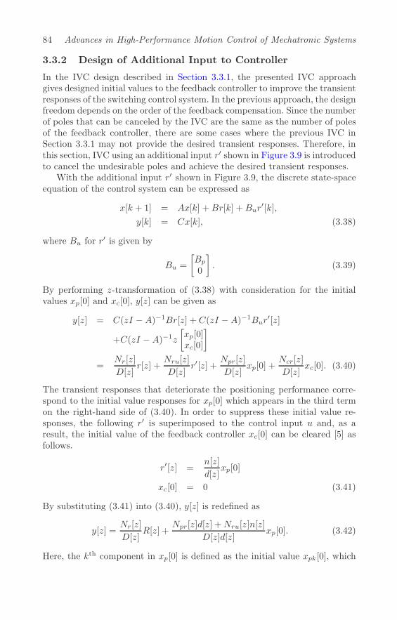
84 Advances in High-Performance Motion Control of Mechatronic Systems
3.3.2 Design of Additional Input to Controller
In the IVC design described in Section 3.3.1, the presented IVC approachgives designed initial values to the feedback controller to improve the transientresponses of the switching control system. In the previous approach, the designfreedom depends on the order of the feedback compensation. Since the numberof poles that can be canceled by the IVC are the same as the number of polesof the feedback controller, there are some cases where the previous IVC inSection 3.3.1 may not provide the desired transient responses. Therefore, inthis section, IVC using an additional input r′ shown in Figure 3.9 is introducedto cancel the undesirable poles and achieve the desired transient responses.
With the additional input r′ shown in Figure 3.9, the discrete state-spaceequation of the control system can be expressed as
x[k + 1] = Ax[k] +Br[k] +Bur′[k],
y[k] = Cx[k], (3.38)
where Bu for r′ is given by
Bu =
[Bp0
]. (3.39)
By performing z-transformation of (3.38) with consideration for the initialvalues xp[0] and xc[0], y[z] can be given as
y[z] = C(zI −A)−1Br[z] + C(zI −A)−1Bur′[z]
+C(zI −A)−1z
[xp[0]xc[0]
]
=Nr[z]
D[z]r[z] +
Nru[z]
D[z]r′[z] +
Npr[z]
D[z]xp[0] +
Ncr[z]
D[z]xc[0]. (3.40)
The transient responses that deteriorate the positioning performance corre-spond to the initial value responses for xp[0] which appears in the third termon the right-hand side of (3.40). In order to suppress these initial value re-sponses, the following r′ is superimposed to the control input u and, as aresult, the initial value of the feedback controller xc[0] can be cleared [5] asfollows.
r′[z] =n[z]
d[z]xp[0]
xc[0] = 0 (3.41)
By substituting (3.41) into (3.40), y[z] is redefined as
y[z] =Nr[z]
D[z]R[z] +
Npr[z]d[z] +Nru[z]n[z]
D[z]d[z]xp[0]. (3.42)
Here, the kth component in xp[0] is defined as the initial value xpk[0], which

Transient Control Using Initial Value Compensation 85
yP [z]
+
+C[z]
+
−r uu′
r′
FIGURE 3.9Block diagram of control system with additional input r′.
should be suppressed by the IVC. The corresponding output y0k[z] for xpk[0]can be extracted as
y0k[z] =Npk[z]d[z] +Nru[z]nk[z]
D[z]d[z]xpk[0], (3.43)
where Npk[z] and nk[z] are the kth polynomials of Np[z] and n[z], respectively.
In IVC using r′, all roots of D[z] can be canceled by designing nk[z], while thedesired poles are assigned by d[z] to allow the initial value responses y0k[z] toconverge to zero by the desired time constant. Therefore, nk[z] can be designedunder the conditions given by
Npk[λi]d[λi] +Nru[λi]nk[λi] = 0, (3.44)
where λi with i = 1, 2, . . . , n+m is the ith root of D[z]. Here, nk[z] is assumedto be represented by the polynomial given by
nk[z] = agzg + ag−1z
g−1 + . . .+ a1z + a0, (3.45)
where ak with k = 0, 1, 2, . . . , g are the undetermined real coefficients. Theequation derived from the combination of (3.44) and (3.45) is given by
⎡⎢⎢⎢⎣
λg1 λg−11 · · · λ1 1
λg2 λg−12 · · · λ2 1
......
......
...
λgn+m λg−1n+m · · · λn+m 1
⎤⎥⎥⎥⎦
⎡⎢⎢⎢⎣
agag−1
...a0
⎤⎥⎥⎥⎦ =
⎡⎢⎢⎢⎣
−Nru[λ1]−1Npk[λ1] d[λ1]−Nru[λ2]−1Npk[λ2] d[λ2]
...−Nru[λn+m]−1Npk[λn+m] d[λn+m]
⎤⎥⎥⎥⎦ . (3.46)
Equation (3.46) can be redefined as
Σa = Γ. (3.47)

86 Advances in High-Performance Motion Control of Mechatronic Systems
The equality constraint of (3.47) to cancel all the roots of D[z] can be definedas an affine function of the free parameter a. The free parameter a can bedetermined by solving (3.47) under the assumptions thatD[z] does not includemultiple roots and g is selected as n+m− 1.
On the other hand, the additional input r′ may cause saturation of thecontrol input u when faster responses are required, which excites the uncer-tain vibration modes in the high frequency range. Therefore, an optimizationapproach for the control input has been developed to design the initial value
compensator nk[z]d[z] [14]. In order to optimize the input, the cost function J
that is to be minimized under the equality constraint of (3.47) is given by [12]
J = aTQxa+ 2Qya+Qz, (3.48)
where Qx, Qy, and Qz are weighting matrices to suppress the amplitude ofthe control input and its jerk component. The control input u[k] in Figure 3.9can be expressed as
u[k] =[−DcCp Cc
] [xp[k]xc[k]
]+Dcr[k] + r′[k]
= Cu
[xp[k]xc[k]
]+Dcr[k] + r′[k]. (3.49)
From (3.15) and (3.49), and by performing z-transformation, u[z] is given as
u[z] = Cu(zI −A)−1Br[z] + (C(zI −A)−1Bu + 1)r′[z]
+Cu(zI −A)−1z
[xp[0]xc[0]
]
=Nu[z]
D[z]r[z] +
Nuu[z]
D[z]r′[z] +
Npu[z]
D[z]xp[0] +
Ncu[z]
D[z]xc[0]. (3.50)
By substituting (3.41) into (3.50), u[z] is given as
u[z] =Nu[z]
D[z]r[z] +
Nuu[z]
D[z]
n[z]
d[z]xp[0] +
Npu[z]
D[z]xp[0]. (3.51)
Using the second and third terms on the right-hand side of (3.51), the corre-sponding control input u0k[z] for xpk[0] can be extracted as
u0k[z] =Nuu[z]
D[z]
nk[z]
d[z]xpk[0] +
Npuk[z]
D[z]xpk[0]. (3.52)
In order to define the cost function J of (3.48), u0k[z] should be expressedas a time series vector U0k ∈ RN×1. Using a controllable canonical form, thecorresponding additional input r′[z] for xpk[0] can be redefined as
r′[z] = Cr(zI −Ar)−1Brxpk[0], (3.53)

Transient Control Using Initial Value Compensation 87
where Ar, Br, and Cr are defined as
Ar =
⎡⎢⎢⎢⎣
0 1 . . . 0
0 0. . . 0
0 0 . . . 1−b0 −b1 . . . −bh
⎤⎥⎥⎥⎦ , Br =
⎡⎢⎢⎢⎣
0...01
⎤⎥⎥⎥⎦ , Cr = aT . (3.54)
Here, (zI − Ar)−1Br is a g × 1 transfer function vector. The unit impulse
response of the i-th transfer function of (zI − Ar)−1Br is defined as V0i ∈
RN×1. As a result, the time series vectorR′ ∈ RN×1 of (3.41) can be expressedas an affine function of a, which is given by
R′ =[V01 V02 . . . V0g
]axpk[0]
= V0axpk[0]. (3.55)
In addition, the unit impulse response Huu ∈ RN×1 of the transfer functionNuu[z]D[z] in (3.52) can be defined as
Huu :=[huu(0) huu(1) . . . huu(N − 1)
]T. (3.56)
A convolution matrix Mu of Huu is defined as [14]
Mu :=
⎡⎢⎢⎢⎣
huu(0) 0 · · · 0huu(1) huu(0) · · · 0
......
. . ....
huu(Nx − 1) huu(Nx − 2) · · · huu(0)
⎤⎥⎥⎥⎦ . (3.57)
Moreover, the unit impulse response of the transfer functionNpuk[z]D[z] is defined
as Ui ∈ RN×1. As a result of the definitions, a time series matrix U0k foru0k[k] can be expressed by Mu, V0, a, and Ui as
U0k = (MuV0ak + Ui)xpk[0]. (3.58)
On the other hand, a differentiation matrix Md ∈ RN×N is defined as
Md :=
⎡⎢⎢⎣
1 0 · · · 0 0−1 1 · · · 0 0· · · · · · · · · · · · · · ·0 0 · · · −1 1
⎤⎥⎥⎦ (3.59)
in order to consider the jerk component in J . A delta matrix J0k for U0k canbe expressed by Md as
J0k = MdU0k
= Md(MuV0a+ Ui)xpk[0]. (3.60)
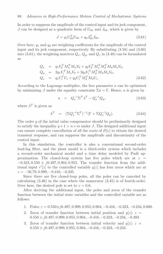
88 Advances in High-Performance Motion Control of Mechatronic Systems
In order to suppress the amplitude of the control input and its jerk component,J can be designed as a quadratic form of U0k and J0k, which is given by
J = q1UT0kU0k + q2J
T0kJ0k. (3.61)
Over here, q1 and q2 are weighting coefficients for the amplitude of the controlinput and its jerk component, respectively. By substituting (3.58) and (3.60)into (3.61), the weighting matrices Qx, Qy, and Qz in (3.48) can be formulatedas
Qx = q1VT0 M
TuMuV0 + q2V
T0 M
TuM
Td MdMuV0,
Qy = 2q1VTi MuV0 + 2q2V
Ti M
Td MdMuV0,
Qz = q1UTi Ui + q2U
Ti M
Td MdUi. (3.62)
According to the Lagrange multiplier, the free parameter a can be optimizedby minimizing J under the equality constraint Σa = Γ. Hence, a is given by
a = Q−1x ΣTλT −Q−1
x Qy, (3.63)
where λT is given as
λT = (ΣQ−1x ΣT )−1(Γ + ΣQ−1
x Qy). (3.64)
The order g of the initial value compensator should be preliminarily designedto satisfy the inequality g+1 > n+m under J . The designed additional inputcan ensure complete cancellation of all the roots of D[z] to obtain the desiredtransient response, and can suppress the amplitude and discontinuity of thecontrol input.
In this simulation, the controller is also a conventional second-orderlead-lag filter, and the plant model is a third-order system which includesa second-order mechanical model and a time delay modeled by Pade ap-proximation. The closed-loop system has five poles which are at z =−0.323, 0.550 ± j0.497, 0.904, 0.955. The transfer function from the addi-tional input r′[z] to the controlled variable y[z] has four zeros which are atz = −56.79, 0.999,−0.416,−0.235.
Since there are five closed-loop poles, all the poles can be canceled bycalculating (3.46) in the case where the numerator (3.45) is of fourth-order.Over here, the desired pole is set to z = 0.6.
After deriving the additional input, the poles and zeros of the transferfunction between the initial state variables and the controlled variable are asfollows:
1. Poles: z = 0.550±j0.497, 0.999, 0.955, 0.904,−0.416,−0.323,−0.234, 0.600.
2. Zeros of transfer function between initial position and y[z]: z =0.550± j0.497, 0.999, 0.955, 0.904,−0.416,−0.323,−0.234,−0.393.
3. Zeros of transfer function between initial velocity and y[z]: z =0.550± j0.497, 0.999, 0.955, 0.904,−0.416,−0.323,−0.234.

Transient Control Using Initial Value Compensation 89
FIGURE 3.10Transient waveforms for various desired eigenvalues (simulation).
All poles except the assigned pole at z = 0.6 are canceled by the zeros.Consequently, the transient response is governed by the assigned pole. Here,the design for initial position and velocity are described in detail. The proce-dure is the same for designing other state variables and references.
Figure 3.10 shows the simulation results for the free responses of threeassigned desired poles at z = 0.4, z = 0.6, and z = 0.8. The trajectories ofthe responses in the phase plane are shown in Figure 3.11, where ‘o’ denotesthe responses of the system, and the solid lines denote the responses of thefirst-order systems with their corresponding poles. The trajectories show thatthe responses are exactly the same as those of the first-order systems.
Figure 3.12 shows the transient responses from both simulations and ex-periments using the HDD head-positioning system. The switching conditionis 6 μm before the target track center, and the velocity is about –10 mm/s.In Figure 3.12, the time responses of the systems, whose individual assignedpoles are respectively z = 0.8, z = 0.6, z = 0.4, and z = 0.2, are shown. Itshould be noted that the transient response can be appropriately designed byassigning a dominant pole. As a result, these figures show that by selecting anappropriate pole, the IVC method improves the settling time by about 2 ms.
3.3.3 Design of Optimal Switching Condition
In this section, a design method for optimizing the mode switching condi-tion is described. As mentioned in the previous sections, IVC is a methodfor improving the characteristics from the initial values at mode switching to

90 Advances in High-Performance Motion Control of Mechatronic Systems
FIGURE 3.11Trajectories on phase plane (simulation).
the control variable such that they are desirable characteristics. However, thisdoes not mean the realization of the desired transient time responses, becausethe transient responses depend on the initial values such as displacement,velocity, and acceleration during mode switching, even though the character-istics between the initial values and the control variable can be shaped ideally.Thus, it is necessary to design an optimal mode switching condition such asan optimal set of initial values during mode switching. By applying IVC, theinitial values during mode switching are only the initial values of the plantmodel. The design of the optimal mode switching condition is the definitionof an index to evaluate a transient time response, and finding a set of initialvalues that minimizes the index. Here, the H2-norm of the displacement re-sponse after mode switching and the H2-norm of the control input responseafter mode switching are defined. It is then necessary to design a referencetrajectory which passes through the designed optimal set of initial values.
The discrete-time state-space equations of a plant P [z] and a controllerC[z] are represented as
P :
{xp[k + 1] = Apxp[k] +Bpu[k]y[k] = Cpxp[k]
, (3.65)
C :
{xc[k + 1] = Acxc[k] +Bc(−y[k])u[k] = Ccxc[k] +Dc(−y[k]) , (3.66)
where xp is a state vector of the plant, xc is a state vector of the controller, uis the control input, y is the control variable, Ap, Bp, and Cp are real matrices
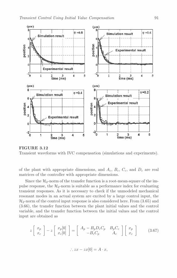
Transient Control Using Initial Value Compensation 91
FIGURE 3.12Transient waveforms with IVC compensation (simulations and experiments).
of the plant with appropriate dimensions, and Ac, Bc, Cc, and Dc are realmatrices of the controller with appropriate dimensions.
Since the H2-norm of the transfer function is a root-mean-square of the im-pulse response, the H2-norm is suitable as a performance index for evaluatingtransient responses. As it is necessary to check if the unmodeled mechanicalresonant modes in an actual system are excited by a large control input, theH2-norm of the control input response is also considered here. From (3.65) and(3.66), the transfer function between the plant initial values and the controlvariable, and the transfer function between the initial values and the controlinput are obtained as
z
[xpxc
]− z
[xp[0]xc[0]
]=
[Ap −BpDcCp BpCc
−BcCp Ac
] [xpxc
](3.67)
∴ zx− zx[0] = A · x,

92 Advances in High-Performance Motion Control of Mechatronic Systems
where x = [xTp xTc ]T , and as a result,
x =
[zI − (Ap −BpDcCp) −BpCc
BcCp zI −Ac
]−1
zx[0], (3.68)
u =[ −DcCc Cc
]x, (3.69)
y =[Cp 0
]x. (3.70)
Next, the IVC is applied to this system. This means that the initial valuesof the controller xc[0] can be replaced by the multiplication of xp[0] with Kwhich can be derived from the IVC algorithm, and where it is assumed thatthe initial values xp[0] of the plant can be measured or estimated. Hence, xc[0]is given by
xc[0] = Kxp[0]. (3.71)
Substituting equation (3.71) into equation (3.68) gives
x =
[zI − (Ap −BpDcCp) −BpCc
BcCp zI −Ac
]−1
z
[IK
]xp[0]. (3.72)
As a result, after using IVC, the transfer function between the plant initialvalues and the control variable, and the transfer function between the plantinitial values and the control input after are
u =[ −DcCc Cc
] [ zI − (Ap −BpDcCp) −BpCcBcCp zI −Ac
]−1
z
[IK
]xp[0]
≡ G · xp[0],(3.73)
y =[Cp 0
] [ zI − (Ap −BpDcCp) −BpCcBcCp zI −Ac
]−1
z
[IK
]xp[0]
≡ H · xp[0].(3.74)
The performance indices are defined as
Ju =‖ G · xp[0] ‖22, (3.75)
Jy =‖ H · xp[0] ‖22 . (3.76)
Next, from the definition of the H2-norm, ‖ G · xp[0] ‖22 becomes
‖ G · xp[0] ‖22 = trace{(xp[0]D)T (Dxp[0]) + (xp[0]B)TLo(Bxp[0])}= trace{xp[0]T (DTD +BTLoB)xp[0]},
(3.77)
where Lo is the solution of the Lyapunov equation in discrete-time domainwhich is given as
ATLoA− Lo + CTC = 0. (3.78)

Transient Control Using Initial Value Compensation 93
For simplicity, the matrices of the state-space equation of G(z) are describedas A, B, C, and D. From (3.77), the optimal combination of the plant statevariables xp(0) can then be calculated by minimizing
xp[0]T (DTD +BTLoB)xp[0]. (3.79)
Since (3.77) is a linear quadratic equation with m variables and the H2-normis positive, the minimum value exists. For example, the state variables of theplant are assumed to be position, velocity, and acceleration, and the initialvalues of the state variables are represented as xp[0] ≡ [xpos xvel xacc]
T .Hence,
Ju = xp[0]T (DTD +BTLoB)xp[0]
≡ xp[0]TKxp[0]
=[xpos xvel xacc
]⎡⎣k11 k12 k13k21 k22 k23k31 k32 k33
⎤⎦⎡⎣xposxvelxacc
⎤⎦ .
(3.80)
The optimal initial condition can then be calculated by solving
∂Ju∂xvel
= 0,∂Ju∂xacc
= 0. (3.81)
The model used in the simulation has open loop characteristics which area crossover frequency of 500 Hz and a phase margin of 36◦. The plant modelis of third-order and the compensator is a conventional second-order lead-lagfilter with a sampling rate of 150 μs.
The H2-norm of u − x[0] for various initial velocities and accelerations isshown in Figure 3.13. It is practical to find a condition with smaller initialvalues, and which does not very much increase the H2-norm.
The experimental setup uses a 3.5′′ HDD. The track-seeking distance isabout 7.5 mm which is one-third of the full stroke, and the mode switch-ing condition is 15 μm from the target track center. During mode switching,pole-zero-type IVC is applied. The experimental and corresponding simulationresults for the transient response of the head position after mode-switchingat t = 0 are shown in Figure 3.14. In each figure, the experimental dataare obtained from many sets of experiments and drawn on the same figure.In Figure 3.14, Condition A represents the responses with a designed mode-switching condition given by an initial velocity of 60 mm/s and an accelerationof 150 m/s2. For comparison, Conditions B and C in Figure 3.14 representworse mode-switching conditions given by initial velocities of 90 mm/s and25 mm/s, respectively. Each condition is plotted in Figure 3.13. It is shownthat the designed mode-switching condition produces the best transient re-sponse. The experimental results for the transient responses of the currentfor the same mode-switching conditions shown in Figure 3.14 are shown inFigure 3.15. It is obvious that the designed mode-switching condition shown

94 Advances in High-Performance Motion Control of Mechatronic Systems
FIGURE 3.13H2-norm plane for initial velocity and acceleration.
in Condition A is the most desirable. From the experimental results of bothposition and current transient responses, it is clear that the proposed mode-switching conditions are appropriate.
Next, the design of the switching condition in consideration of constraintsis explained [2, 3]. The discrete-time state-space equations of a plant P and acontroller C are represented as (3.65) and (3.66), respectively. To ensure thatbumpy switching does not occur, the constraint imposed on the control inputu after switching is given by
−0.02 ≤ u[k] ≤ 0.02, k ≥ 0, (3.82)
where the control input u refers to current in the case of the Voice Coil Motor(VCM). The vector signal to be constrained is expressed as z which is equalto u. Z represents the set of z which satisfies the specified constraints and isgiven by
Z = {z| Mzz ≤ mz} , (3.83)
where
Mz =
[ −11
], mz =
[0.020.02
], (3.84)
and where it is assumed that Z includes the origin. The state-space equationof the closed-loop system is expressed as
⎧⎨⎩
x[k + 1] = Ax[k]y[k] = Cx[k]z[k] = Czx[k]
, (3.85)

Transient Control Using Initial Value Compensation 95
FIGURE 3.14Transient response of head position after mode switching (experimental re-sults).
1 2 3 4
-0.5
0
0.5
1
time (ms)
-10
-10
-10
-10
-10
-100 1 2 3 4
-1
-0.5
0
0.5
1
time (ms)0000000000 1 2 3 4
-1
-0.5
0
0.5
1
time (ms)0000000000
(A)
Cur
rent
Switching condition: A Switching condition: B Switching condition: C
(A) (A)
Cur
rent
Cur
rent
FIGURE 3.15Transient response of current after mode switching (experimental results).
where
x[k] =
[xp[k]xc[k]
], A =
[Ap −BpDcCp BpCc
−BcCp Ac
], (3.86)
C =[Cp 0
], Cz =
[ −DcCp Cc]. (3.87)
The vector signal z to be constrained at time k can be expressed as
z[k] = CzAkx[0] = CzA
k
[xp[0]xc[0]
]. (3.88)
Thus, the maximal output admissible set O∞ is defined as
O∞ =
{x[0] =
[xp[0]xc[0]
]| z[k] ∈ Z, k ≥ 0
}. (3.89)
The maximal output admissible set O∞ is a set of all closed-loop initial states

96 Advances in High-Performance Motion Control of Mechatronic Systems
which can be converged to the origin without violating the specified constraintsdefined in (3.83). In order to improve the transient response after switching,J-min-type IVC is applied as
xc[0] = Kxp[0], (3.90)
where K ∈ Rm×n is the real coefficient matrix to be designed. To preventbumpy switching, the cost function of IVC is defined as
J =
∞∑k=0
u[k]2. (3.91)
By using IVC, (3.89) can be tranformed as
O∞ =
{x[0] =
[IK
]xp[0]| z[k] ∈ Z, k ≥ 0
}. (3.92)
The safe switching condition so that the given constraints are fulfilled can bedesigned by calculating the maximal output admissible set O∞.
The calculated maximal output admissible set is shown in Figure 3.16. Thesolid line is where the initial state of the controller is initialized by the IVCtechnique, and the dashed line is where the initial state of the controller is setto zero. The horizontal axis represents the head position normalized by thetrack-pitch which is denoted as Tp, and the vertical axis represents the headvelocity. The origin of the horizontal axis represents the target track position.For instance, –10 on the horizontal axis represents the position of 10 tracksahead of the target track. The safe region where the constraints are fulfilledis expanded using the IVC technique.
The simulation results for initializations using IVC and zero reset case areshown in Figures 3.17 and 3.18, respectively. The four switching conditionslisted in Table 3.1 are evaluated for the simulation. The relation between themaximal output admissible set and the four switching conditions is shown inFigure 3.16. For the initialization using IVC, it is shown in Figure 3.17 thatthe constraint on the control input is fulfilled when the switching conditionsare contained within the maximal output admissible set. For all switchingconditions, the transient response of the positioning error is good. On theother hand, only switching condition 1 is contained within the maximal outputadmissible set for initialization using zero reset, and the results in Figure 3.18show that the constraint on the control input is fulfilled only for switchingcondition 1. However, even when the switching condition is contained withinthe maximal output admissible set, the positioning error does not have a goodtransient response, i.e., an overshoot occurs.
The experimental results for the initialization using IVC are shown in Fig-ure 3.19. Switching condition 2 listed in Table 1 is used. Figure 3.19(a) isa plot of the entire control input waveform, Figure 3.19(b) is a close-up ofFigure 3.19(a), and Figure 3.19(c) is a plot of the positioning error waveform
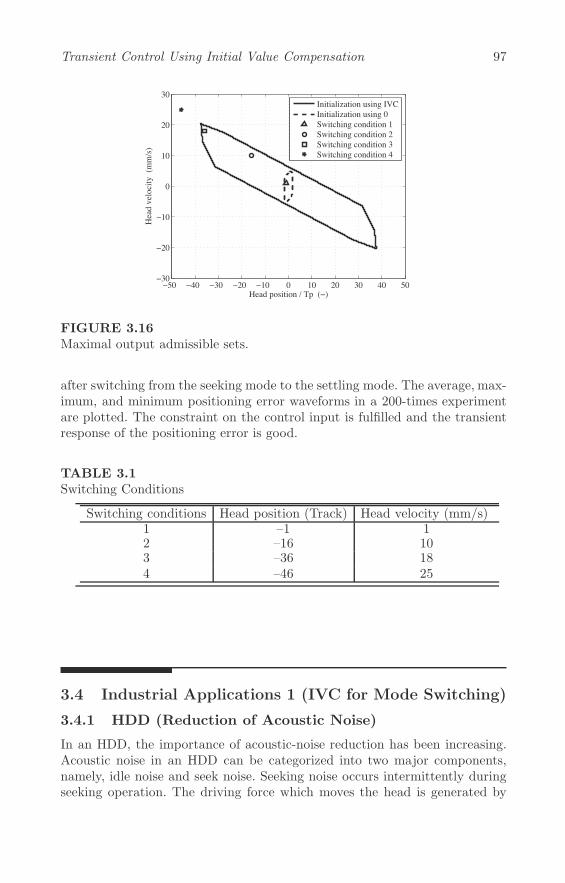
Transient Control Using Initial Value Compensation 97
−50 −40 −30 −20 −10 0 10 20 30 40 50−30
−20
−10
0
10
20
30
Head position / Tp (−)
Hea
d ve
loci
ty (
mm
/s)
Initialization using IVCInitialization using 0Switching condition 1Switching condition 2Switching condition 3Switching condition 4
FIGURE 3.16Maximal output admissible sets.
after switching from the seeking mode to the settling mode. The average, max-imum, and minimum positioning error waveforms in a 200-times experimentare plotted. The constraint on the control input is fulfilled and the transientresponse of the positioning error is good.
TABLE 3.1Switching Conditions
Switching conditions Head position (Track) Head velocity (mm/s)1 –1 12 –16 103 –36 184 –46 25
3.4 Industrial Applications 1 (IVC for Mode Switching)
3.4.1 HDD (Reduction of Acoustic Noise)
In an HDD, the importance of acoustic-noise reduction has been increasing.Acoustic noise in an HDD can be categorized into two major components,namely, idle noise and seek noise. Seeking noise occurs intermittently duringseeking operation. The driving force which moves the head is generated by

98 Advances in High-Performance Motion Control of Mechatronic Systems
supplying a current to the VCM. When the VCM moves the head, mechanicalvibrations may occur in the HDD depending on the waveform of the VCMforce. These vibrations spread to the top cover. It is considered that the vi-bration of the top cover in contact with external air is the main cause ofseeking noise. Therefore, to reduce the seeking noise, it is necessary to opti-mize the seeking current. In particular, discontinuous switching from modeswitching control excites the mechanical resonant modes and increases theacoustic noise. Thus, an example of switching condition design which is basedon the IVC method and reduces seek noise is explained [2, 3].
The block diagram of the model-following control system for the settlingmode is shown in Figure 3.20. P is the plant, P0 is the plant model, C is afollowing controller, C0 is a settling controller, u0 ∈ R is the control input,y0 ∈ R is the controlled variable which is the head position, and r ∈ R is thereference. The discrete-time state-space equations of the plant model P0 andthe settling controller C0 are represented as
P0 :
{xp0[k + 1] = Ap0xp0[k] +Bp0u0[k]y0[k] = Cp0xp0[k]
, (3.93)
C0 :
{xc0[k + 1] = Ac0xc0[k] +Bc0(r[k]− y0[k])u0[k] = Cc0xc0[k] +Dc0(r[k] − y0[k])
, (3.94)
where xp0 ∈ Rn×1 is a state vector of the plant, xc0 ∈ Rm×1 is a state vector ofthe settling controller, Ap0, Bp0, and Cp0 are real matrices of the plant modelwith appropriate dimensions, and Ac0, Bc0, Cc0, and Dc0 are real matrices ofthe settling controller with appropriate dimensions. During mode switchingfrom seeking mode to settling mode, the model-following control operates asfollows: (1) IVC is applied to the settling controller C0; (2) The initial state ofthe following controller C is set to zero; and (3) The initial state of the plantmodel P0 is set to the initial state xp[0] of the actual plant. Consequently,when the mode switches from settling mode to following mode, the controllerremains switched on. Therefore, mode switching is carried out once from theseeking mode to the settling mode.
To reduce the seeking noise, it is necessary to reduce the impulse-likecurrent at mode switching. Therefore, a cost function for the J-min-type IVCis defined as
J =∞∑k=0
u20[k]
=
∞∑k=0
[xTp0[k] xTc0[k]
]Q
[xp0[k]xc0[k]
],
(3.95)
whereQ =
[ −Dc0Cp0 Cc0]T [ −Dc0Cp0 Cc0
]. (3.96)
In order to achieve the effects of the IVC method, the design of switching

Transient Control Using Initial Value Compensation 99
conditions is also carried out. By using the IVC method, the initial stateof the settling controller is produced by the initial state of the plant. Thus,the state of the closed-loop system only becomes the state of the plant andtherefore, the switching conditions are simple. In addition, velocity control isperformed so that the acceleration may be set to zero at the termination ofthe seeking mode. As a result, in terms of the state variables of the plant, thedeciding of the switching condition from seeking mode to settling mode is theproblem of finding an optimal combination of position and velocity.
The design of the switching conditions is performed using the followingprocedures: (1) The index for evaluating the control purpose is set up. Thetrade-off between the peak value of operation current (which is an importantfactor in the reduction of acoustic noise during seek), the overshoot of thehead position, and the settling-time after mode switching is considered; (2)The initial states which are guaranteed to satisfy the constraints given to eachevaluation index are calculated; and (3) According to the calculated initialstate sets, the switching conditions are determined with consideration for thetrade-off of each evaluation index.
The initial state sets that meet their individual constraint condition on thecurrent peak value cp are shown in Figure 3.21. Figure 3.21(a) is a plot for thepole-zero-type IVC for comparison, and Figure 3.21(b) is a plot for the J-min-type IVC. The horizontal axis represents the head position normalized by thetrack-pitch which is denoted as Tp, and the vertical axis represents the headvelocity. The origin of the horizontal axis represents the target track position.For instance, –10 of the horizontal axis shows the position of 10 tracks forwardfrom the target track. By using the J-min-type IVC technique, the safe regionwhere the current peak value is reduced is expanded. The switching conditionscan be chosen from within the safe region.
The initial state sets that meet their individual constraint condition onthe overshoot os are shown in Figure 3.22. Both the pole-zero-type IVC andthe J-min-type IVC have a large safe region where the overshoot of the headposition is reduced to 10% or less of the track pitch.
Figure 3.23 shows the initial state sets that meet their individual constraintcondition on the settling time st which is defined as the time required forthe positioning error to converge to less than 10% of the track pitch. Thesafe region where the constraint on the settling time is fulfilled is small forboth the pole-zero-type IVC and the J-min-type IVC. From the perspectiveof reducing acoustic noise, J-min type IVC may have broader alternatives indesigning IVC.
The experimental results for the pole-zero-type IVC and the J-min-type IVC are shown in Figures 3.24 and 3.25, respectively. Figures 3.24(a)and 3.25(a) are plots of operation current, and Figures 3.24(b) and 3.25(b)are plots of sound pressure normalized by its maximum value. The switchingcondition is determined in consideration of the calculated initial state sets,which is given by a position of 16 tracks forward from the target track and avelocity of 10 mm/s. By using the J-min-type IVC with the optimal switching

100 Advances in High-Performance Motion Control of Mechatronic Systems
condition, the impulse-like current at mode switching is reduced and therefore,the sound pressure is also reduced.
3.4.2 Robot (Personal Mobility Robot)
3.4.2.1 Introduction
Recently, several types of Personal Mobility Robot (PMR) for our aging so-ciety are being developed to travel a short distance [39]. The PMR shown inFigure 3.26 is a wheeled inverted pendulum type mobility robot which cantravel and control its posture using two driven wheels. Also, there is a joystickas a human-machine interface, a gyro sensor to control its posture, a seat, apair of assist wheels, and a footrest. Wheeled inverted pendulum type mobil-ity has various advantages in traveling performance as compared to electricwheelchair type mobility whose four wheels are always in contact with theground. For example, the PMR can turn about a point and can maintainthe same seat posture even on a slope. However, the PMR also has its dis-advantages. Wheeled inverted pendulum type mobility must be stabilized bya feedback controller in order to maintain the posture of the body. Further-more, the body is easily swung, no matter what the controller is. Therefore,the PMR must be steadied by additional assist wheels on the ground whena driver mounts, dismounts, or works from the PMR. In order to accomplishboth of the above tasks, the traveling mode of the PMR must be switchedbetween the four-wheel mode and the wheeled inverted pendulum mode de-pending on the situations [40].
Transient Control Using Initial Value Compensation 101
0 1 2 3 4 5−0.04
−0.03
−0.02
−0.01
0
0.01
0.02
0.03
0.04
Time (ms)
Con
trol i
nput
(A
)
Switching condition 1Switching condition 2Switching condition 3Switching condition 4
(a) Control input
0 1 2 3 4 5−2
−1.5
−1
−0.5
0
0.5
1
1.5
2
Time (ms)
Posi
tioni
ng e
rror
(Tr
ack)
Switching condition 1Switching condition 2Switching condition 3Switching condition 4
(b) Positioning error
FIGURE 3.17Simulations results for initialization using IVC.

102 Advances in High-Performance Motion Control of Mechatronic Systems
0 1 2 3 4 5−0.04
−0.03
−0.02
−0.01
0
0.01
0.02
0.03
0.04
Time (ms)
Con
trol i
nput
(A
)
Switching condition 1Switching condition 2Switching condition 3Switching condition 4
(a) Control input
0 1 2 3 4 5−2
−1.5
−1
−0.5
0
0.5
1
1.5
2
Time (ms)
Posi
tioni
ng e
rror
(Tr
ack)
Switching condition 1Switching condition 2Switching condition 3Switching condition 4
(b) Positioning error
FIGURE 3.18Simulation results for initialization using zero reset.
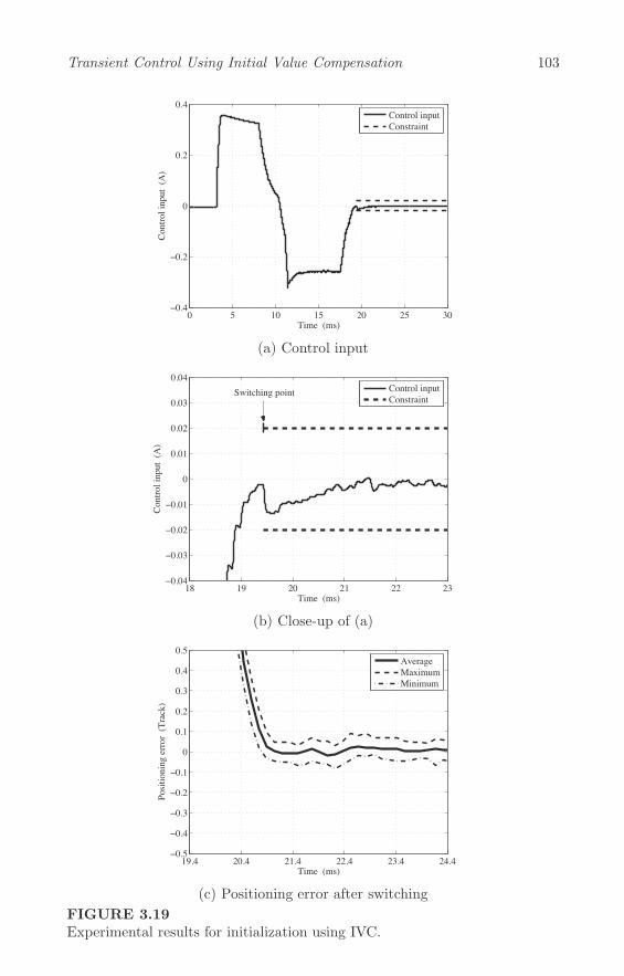
Transient Control Using Initial Value Compensation 103
0 5 10 15 20 25 30−0.4
−0.2
0
0.2
0.4
Time (ms)
Con
trol i
nput
(A
)
Control inputConstraint
(a) Control input
18 19 20 21 22 23−0.04
−0.03
−0.02
−0.01
0
0.01
0.02
0.03
0.04
Time (ms)
Con
trol i
nput
(A
)
Control inputConstraint
Switching point
(b) Close-up of (a)
19.4 20.4 21.4 22.4 23.4 24.4−0.5
−0.4
−0.3
−0.2
−0.1
0
0.1
0.2
0.3
0.4
0.5
Time (ms)
Posi
tioni
ng e
rror
(Tr
ack)
AverageMaximumMinimum
(c) Positioning error after switching
FIGURE 3.19Experimental results for initialization using IVC.

104 Advances in High-Performance Motion Control of Mechatronic Systems
ZOH
IVC
C0 P0
C P
r u0 y0
FIGURE 3.20Block diagram of model-following control system with IVC.
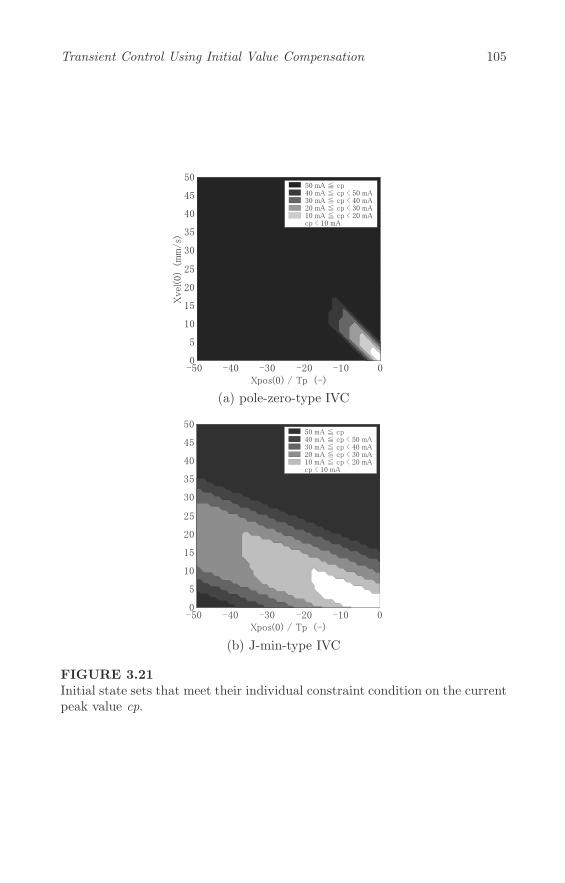
Transient Control Using Initial Value Compensation 105
-50 -40 -30 -20 -10 00
5
10
15
20
25
30
35
40
45
50
Xpos(0) / Tp (-)
Xvel(0)
(m
m/s)
50 mA ≦ cp
40 mA ≦ cp < 50 mA
30 mA ≦ cp < 40 mA
20 mA ≦ cp < 30 mA
10 mA ≦ cp < 20 mA
cp < 10 mA
(a) pole-zero-type IVC
(b) J-min-type IVC
FIGURE 3.21Initial state sets that meet their individual constraint condition on the currentpeak value cp.

106 Advances in High-Performance Motion Control of Mechatronic Systems
-50 -40 -30 -20 -10 00
5
10
15
20
25
30
35
40
45
50
Xpos(0) / Tp (-)
Xvel(0)
(m
m/s)
80 % ≦ os
60 % ≦ os < 80 %
40 % ≦ os < 60 %
20 % ≦ os < 40 %
10 % ≦ os < 20 %
os < 10 %
(a) pole-zero-type IVC
(b) J-min-type IVC
FIGURE 3.22Initial state sets that meet their individual constraint condition on the over-shoot os.
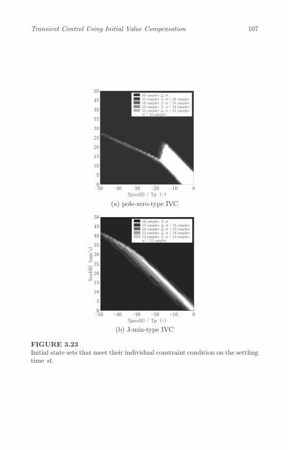
Transient Control Using Initial Value Compensation 107
(a) pole-zero-type IVC
-50 -40 -30 -20 -10 00
5
10
15
20
25
30
35
40
45
50
Xpos(0) / Tp (-)
Xvel(0)
(m
m/s)
16 samples ≦ st
15 samples ≦ st < 16 samples
14 samples ≦ st < 15 samples
13 samples ≦ st < 14 samples
12 samples ≦ st < 13 samples
st < 12 samples
(b) J-min-type IVC
FIGURE 3.23Initial state sets that meet their individual constraint condition on the settlingtime st.

108 Advances in High-Performance Motion Control of Mechatronic Systems
0 5 10 15 20 25 30 35−0.4
−0.2
0
0.2
0.4
Time [ms]
Cur
rent
[A
]
(a) Current
0 5 10 15 20 25 30 35−0.4
−0.2
0
0.2
0.4
Time [ms]
Soun
d pr
essu
re
(b) Sound pressure
FIGURE 3.24Experimental results for pole-zero-type IVC.
0 5 10 15 20 25 30 35−0.4
−0.2
0
0.2
0.4
Time [ms]
Cur
rent
[A
]
(a) Current
0 5 10 15 20 25 30 35−0.4
−0.2
0
0.2
0.4
Time [ms]
Soun
d pr
essu
re
(b) Sound pressure
FIGURE 3.25Experimental results for J-min-type IVC.

Transient Control Using Initial Value Compensation 109
FIGURE 3.26Configuration of prototype PMR.
An example of a transition from the four-wheel mode to the wheeled in-verted pendulum mode is shown in Figure 3.27. In Figure 3.27(a), the PMRrests on four wheels to allow mounting, dismounting, or work to be carriedout safely while sitting down. In this transition example, the PMR acceler-ates to raise the two front assistant wheels as shown in Figure 3.27(b). Next,its wheelie-like state is detected by the internal gyroscope. Based on thisdetection, the feedback controller for the wheeled inverted pendulum modestabilizes its posture. As a result, the PMR can travel safely. From the aboveexaminations, the three important issues that should be solved to realize thetransition are as follows:
(a) To design an acceleration pattern to raise the assistant wheels;
(b) To distinguish whether the assistant wheels are in contact with theground or not; and
(c) To smoothly switch to the feedback controller.
For (c), an appropriate initial value of the feedback controller for the wheeledinverted pendulum mode should be designed and given to improve the ridequality during switching. Therefore, the IVC presented in Section 3.3.1 isapplied to achieve the required specifications. In addition, simple solutionsare given for (a) and (b) in this section. For (a), a stepwise torque referenceis generated. Its amplitude is given as a sufficient value to raise the assistantwheels independent of the driver. For (b), the state of the PMR is determinedby the threshold of inclination angle η = 0.05 rad for the PMR.

110 Advances in High-Performance Motion Control of Mechatronic Systems
(a)
η η
(c)(b)
FIGURE 3.27Transition from four-wheel mode to wheeled inverted pendulum mode.
3.4.2.2 Mathematical Model
The basic model for the wheeled inverted pendulum mode is shown in Fig-ure 3.28. Using the Lagrange equation of motion, the mathematical model forthe wheeled inverted pendulum mode can be formulated as
(Mbl2 + Jb + n2Jm)η(t) + (Mbrwl − n2Jm)θ(t)
−Mbglsinη(t) + fr(η(t)− θ(t)) = −nτ(t),
(Mbrwl − n2Jm)η(t) + ((Mb +Mw)r2w
+Jw + n2Jm))θ(t) − Mblrwη(t)2sinη(t)η(t)
− fr(η(t)− θ(t)) = nτ(t),
(3.97)
whereMw, Jw, and rw are the weight, inertia, and radius of each driven wheel,respectively, Jm is the inertia of the motor, n is the gear ratio, Mb and Jb arethe total weight and total inertia of the human and the PMR without thedriven wheels, respectively. The human together with the PMR without thedriven wheels is referred to as the upper body, and l in (3.97) is the distancebetween the axle and the center of gravity of the upper body, θ is the angleof the driven wheel, η is the inclination angle of the upper body, fr is theviscosity coefficient, and g is acceleration of gravity. In order to apply IVC tothis system, (3.97) can be linearized under the assumption of η(t) � 1, andit is given by
(Mbl2 + Jb + n2Jm)η(t) + (Mbrwl − n2Jm)θ(t)
−Mbglη(t) + fr(η(t)− θ(t)) = −nτ(t),
(Mbrwl − n2Jm)η(t) + ((Mb +Mw)r2w
+Jw + n2Jm))θ(t) − fr(η(t)− θ(t)) = nτ(t). (3.98)

Transient Control Using Initial Value Compensation 111
lθ
η
rw
Mb
Mw Jw
Jb
FIGURE 3.28Model of wheeled inverted pendulum mode of PMR.
+
−r
C[z]P [z]
η
yuw
u
FIGURE 3.29Block diagram of switching control system for making transition between thefour-wheel mode and the wheeled inverted pendulum mode.
The block diagram of the switching control system for making the transitionfrom the four-wheel mode to the wheeled inverted pendulum mode is shownin Figure 3.29. Over here, P [z] is the transfer function from torque inputu = nτ for the driving wheels to y = [η[k] η[k] θ[k] − η[k]]T , C[z] is a fifth-order feedback compensator designed by H∞ control framework to stabilizethe unstable plant system P [z], r is the reference for y, and uw is the torqueinput for the four-wheeled mode.
3.4.2.3 Design of IVC
The order of the feedback compensator C[z] is enough to improve the transientresponses by mode switching with the IVC in Section 3.3.1. The initial valuexc[0] for the feedback compensator C[z] can be optimized by the minimization

112 Advances in High-Performance Motion Control of Mechatronic Systems
of the following cost function J given by [33]
J = Js + quJu + qjJj , (3.99)
where Js is a cost function for converging the state values to those at steadystate, Ju is a cost function for decreasing the amplitude of the control input,Jj is a cost function for suppressing the jerk component, and qu and qj are theweighting coefficients for each cost function. This cost function can be derivedas the square of xc[0]. The appropriate initial value xc[0] can be given as
xc[0] = Kaxp[0] +Kbr +Kcuw, (3.100)
where xp[0] is the initial value of P [z], and Ka, Kb, and Kc are the matrixcoefficients designed by minimizing J . As a result, the transient responses canbe improved only by providing the designed xc[0] for the feedback compensatorC[z] during switching [33].
3.4.2.4 Experimental Results
The experimental results with and without the IVC are shown in Figure 3.30,in which a driver actually mounts a prototype of the PMR. Figure 3.30(a)shows the waveforms of motor velocity x = θ − η, Figure 3.30(b) shows thewaveforms of inclination angle η, Figure 3.30(c) shows the waveforms of incli-nation angular velocity η, and Figure 3.30(d) shows the waveforms of controlinput τ . The horizontal dotted line in Figure 3.30(a) indicates the target valueof the motor velocity which corresponds to 1.0 km/h. In Figures 3.30(a)–(d),the vertical dashed lines indicate the switching time of the feedback controller,which is defined as 0 s. Before switching, a stepwise control input is given toaccelerate the PMR and lift the assist wheels. Therefore, the inclination angleη shown in Figure 3.30(b) decreases and reaches the threshold value η = 0.05which is used to determine whether the assist wheels are in contact with theground or not. After switching, the gray lines in Figures 3.30(a)–(c) indicatethat without IVC, there are large overshoot and undershoot in the responsesof the motor velocity, the inclination angle, and the inclination angular veloc-ity. In addition, the control input τ suddenly decreases and reaches −20 Nmjust after switching, after which τ increases to +20 Nm with an oscillatoryresponse.
On the other hand, it is shown by the solid lines that with IVC, all tran-sient responses converge smoothly to their steady states without overshoot orundershoot, while the amplitude and jerk component of the control input aresuppressed.
In order to evaluate the ride quality of the proposed approach, the accelera-tions of the driver’s head in both horizontal and vertical directions are detectedby acceleration sensors. The waveforms of the acceleration in both horizontaland vertical directions are shown in Figure 3.31. Figure 3.31(a) shows that themaximum value of acceleration in the horizontal direction is 7.0 m/s2 with-out IVC, while acceleration in the horizontal direction is suppressed to within
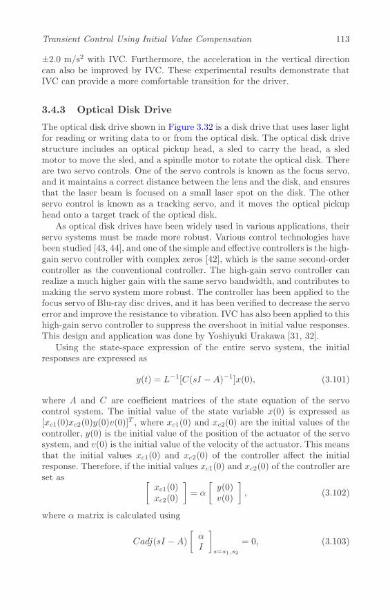
Transient Control Using Initial Value Compensation 113
±2.0 m/s2 with IVC. Furthermore, the acceleration in the vertical directioncan also be improved by IVC. These experimental results demonstrate thatIVC can provide a more comfortable transition for the driver.
3.4.3 Optical Disk Drive
The optical disk drive shown in Figure 3.32 is a disk drive that uses laser lightfor reading or writing data to or from the optical disk. The optical disk drivestructure includes an optical pickup head, a sled to carry the head, a sledmotor to move the sled, and a spindle motor to rotate the optical disk. Thereare two servo controls. One of the servo controls is known as the focus servo,and it maintains a correct distance between the lens and the disk, and ensuresthat the laser beam is focused on a small laser spot on the disk. The otherservo control is known as a tracking servo, and it moves the optical pickuphead onto a target track of the optical disk.
As optical disk drives have been widely used in various applications, theirservo systems must be made more robust. Various control technologies havebeen studied [43, 44], and one of the simple and effective controllers is the high-gain servo controller with complex zeros [42], which is the same second-ordercontroller as the conventional controller. The high-gain servo controller canrealize a much higher gain with the same servo bandwidth, and contributes tomaking the servo system more robust. The controller has been applied to thefocus servo of Blu-ray disc drives, and it has been verified to decrease the servoerror and improve the resistance to vibration. IVC has also been applied to thishigh-gain servo controller to suppress the overshoot in initial value responses.This design and application was done by Yoshiyuki Urakawa [31, 32].
Using the state-space expression of the entire servo system, the initialresponses are expressed as
y(t) = L−1[C(sI −A)−1]x(0), (3.101)
where A and C are coefficient matrices of the state equation of the servocontrol system. The initial value of the state variable x(0) is expressed as[xc1(0)xc2(0)y(0)v(0)]
T , where xc1(0) and xc2(0) are the initial values of thecontroller, y(0) is the initial value of the position of the actuator of the servosystem, and v(0) is the initial value of the velocity of the actuator. This meansthat the initial values xc1(0) and xc2(0) of the controller affect the initialresponse. Therefore, if the initial values xc1(0) and xc2(0) of the controller areset as [
xc1(0)xc2(0)
]= α
[y(0)v(0)
], (3.102)
where α matrix is calculated using
Cadj(sI −A)
[αI
]
s=s1,s2
= 0, (3.103)
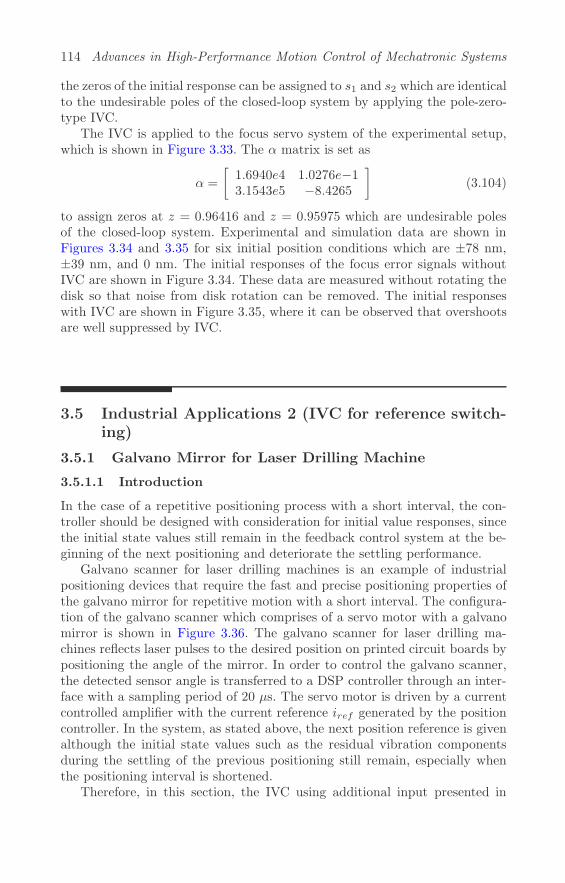
114 Advances in High-Performance Motion Control of Mechatronic Systems
the zeros of the initial response can be assigned to s1 and s2 which are identicalto the undesirable poles of the closed-loop system by applying the pole-zero-type IVC.
The IVC is applied to the focus servo system of the experimental setup,which is shown in Figure 3.33. The α matrix is set as
α =
[1.6940e4 1.0276e−13.1543e5 −8.4265
](3.104)
to assign zeros at z = 0.96416 and z = 0.95975 which are undesirable polesof the closed-loop system. Experimental and simulation data are shown inFigures 3.34 and 3.35 for six initial position conditions which are ±78 nm,±39 nm, and 0 nm. The initial responses of the focus error signals withoutIVC are shown in Figure 3.34. These data are measured without rotating thedisk so that noise from disk rotation can be removed. The initial responseswith IVC are shown in Figure 3.35, where it can be observed that overshootsare well suppressed by IVC.
3.5 Industrial Applications 2 (IVC for reference switch-ing)
3.5.1 Galvano Mirror for Laser Drilling Machine
3.5.1.1 Introduction
In the case of a repetitive positioning process with a short interval, the con-troller should be designed with consideration for initial value responses, sincethe initial state values still remain in the feedback control system at the be-ginning of the next positioning and deteriorate the settling performance.
Galvano scanner for laser drilling machines is an example of industrialpositioning devices that require the fast and precise positioning properties ofthe galvano mirror for repetitive motion with a short interval. The configura-tion of the galvano scanner which comprises of a servo motor with a galvanomirror is shown in Figure 3.36. The galvano scanner for laser drilling ma-chines reflects laser pulses to the desired position on printed circuit boards bypositioning the angle of the mirror. In order to control the galvano scanner,the detected sensor angle is transferred to a DSP controller through an inter-face with a sampling period of 20 μs. The servo motor is driven by a currentcontrolled amplifier with the current reference iref generated by the positioncontroller. In the system, as stated above, the next position reference is givenalthough the initial state values such as the residual vibration componentsduring the settling of the previous positioning still remain, especially whenthe positioning interval is shortened.
Therefore, in this section, the IVC using additional input presented in
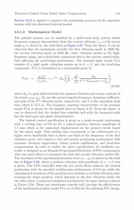
Transient Control Using Initial Value Compensation 115
Section 3.3.2 is applied to improve the positioning accuracy of the repetitivemotion with the shortened interval period.
3.5.1.2 Mathematical Model
The galvano scanner can be modeled by a multi-mass body system whosefrequency response characteristic from the current reference iref to the motorangle ys is shown by the solid lines in Figure 3.37. From the figure, it can beobserved that the mechanism includes the first vibration mode at 3020 Hz,the second vibration mode at 6240 Hz, other vibration modes in the high-frequency range, and a dead-time component due to the current control delay,thus affecting the positioning performance. The nominal plant model P (s)consists of a rigid mode, vibration modes up to k = 2, and the dead-timecomponent. P (s) is formulated as a polynomial given by
P (s) =ys(s)
iref(s)= e−Ls ·Kp
(1
s2+
2∑k=1
Kk
s2 + 2ζnkωnks+ ω2nk
),
(3.105)
whereKp is a gain which includes the moment of inertia and torque constant ofthe motor, ωnk, ζnk,Kk are the natural angular frequency, damping coefficient,and gain of the kth vibration mode, respectively, and L is the equivalent deadtime which is 15.5 μs. The frequency response characteristic of the nominalmodel P (s) is shown by the dashed lines in Figure 3.37. From the figure, itcan be observed that the dashed line coincides well with the measured solidline for both gain and phase characteristics.
The desired control specification is given as a point-to-point positioningwith a settling time of 0.9 ms for a typical position reference amplitude of1.5 mm which is the equivalent displacement on the printed circuit boardfor the motor angle. This settling time corresponds to the achievement of ahigher servo bandwidth that is above one-third of the frequency of the firstvibration mode, and requires a fast and precise positioning performance withresonant vibration suppression, robust system stabilization, and dead-timecompensation. In order to realize the above specification, the feedback con-troller is designed as an Integral-Proportional-Derivative (I-PD) compensatorwith two notch filters to attenuate the first and second vibration modes [35].The waveform of the experimental position error (xr−ys) is shown by the solidline in Figure 3.38, where a position reference with amplitude of xr =1.5 mmis given. The I-PD controller with the two notch filters achieves the desiredpositioning with the specified settling-time performance of 0.9 ms, while theexperimental waveform of the position error includes a residual vibration afterreaching the target position, which depends on the first vibration mode. Onthe other hand, a numerical simulated waveform for the same motion is shownin Figure 3.38. These two waveforms coincide well, proving the effectivenessof the mathematical plant model P (s) in (3.105) for the following IVC design.

116 Advances in High-Performance Motion Control of Mechatronic Systems
It is important for the galvano scanner to provide the desired fast and pre-cise positioning performance for arbitrary repetitive position references withshort interval periods. Although the waveform for a single-reference motioncan satisfy the control specification as shown in Figure 3.38, the expansionof the servo bandwidth excites the residual vibration corresponding to thefirst vibration mode, which directly affects the initial values and hence thesettling characteristics of the next motion. Over here, the positioning perfor-mance is examined for a sequential back-and-forth positioning motion between0 and 1.5 mm. An example of the experimental position error waveforms forthe repetitive reference with the typical interval period of 1.5 ms is shownin Figure 3.39, where Figure 3.39(b) shows eight superimposed trials of theback-and-forth waveform. In Figure 3.39(b), the left waveforms correspond tothe responses of the forward motion, and the right waveforms after 1.5 mscorrespond to the responses of the backward motion. It should be noted thatthe thick line among the left waveforms in Figure 3.39(b) represents the re-sponse of the first motion with zero initial values, which satisfies the desiredpositioning. On the other hand, other waveforms in Figure 3.39(b) includescattered residual vibrations due to the undesirable initial values correspond-ing to the first vibration mode, which deteriorate the positioning accuracy. Inaddition, the experimental results with a shorter interval period of 1.16 msare also shown in Figure 3.40. In the same way as that shown in Figure 3.39,the undesirable initial values lead to scattered residual vibrations after thesecond positioning.

Transient Control Using Initial Value Compensation 117
−0.5 0 0.5 1 1.5 2−2
0
2
4
6
8
time [s]
mot
or v
eloc
ity [r
ad/s
]
−0.5 0 0.5 1 1.5 2−0.1
−0.05
0
0.05
0.1
0.15
time [s]
η [r
ad]
−0.5 0 0.5 1 1.5 2−0.5
0
0.5
time [s]
angu
lar v
el. o
f η
[rad
/s]
−0.5 0 0.5 1 1.5 2−30
−20
−10
0
10
20
30
time [s]
cont
rol i
nput
τ [N
m]
w/o IVCwith IVC
w/o IVCwith IVC
w/o IVCwith IVC
w/o IVCwith IVC
[a]
[b]
[c]
[d]
FIGURE 3.30Experimental results with and without IVC.

118 Advances in High-Performance Motion Control of Mechatronic Systems
−0.5 0 0.5 1 1.5 2−4
−2
0
2
4
6
8
10
time [s]
acce
lera
tion
for
horiz
onta
l axi
s [m
/s2 ]
−0.5 0 0.5 1 1.5 27
8
9
10
11
12
time [s]
acce
lera
tion
for
verti
cal a
xis [
m/s2 ]
w/o IVCwith IVC
w/o IVCwith IVC
[a]
[b]
FIGURE 3.31Experimental results for acceleration of driver’s head.
FIGURE 3.32Schematic apparatus of an optical disk drive.

Transient Control Using Initial Value Compensation 119
FIGURE 3.33Focus servo system of the experimental setup with the high-gain servo con-troller [32].
FIGURE 3.34Initial responses of the focus servo system of the experimental setup withoutIVC [32].
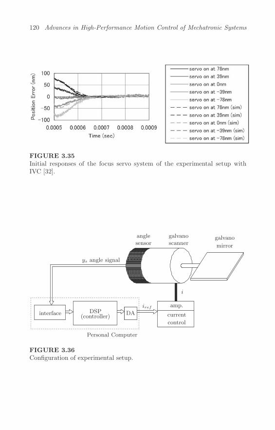
120 Advances in High-Performance Motion Control of Mechatronic Systems
FIGURE 3.35Initial responses of the focus servo system of the experimental setup withIVC [32].
ys angle signal
galvanoscanner
control
currentDA(controller)
DSP
Personal Computer
amp.iref
i
interface
anglesensor mirror
galvano
FIGURE 3.36Configuration of experimental setup.

Transient Control Using Initial Value Compensation 121
103
104
-100
-80
-60
-40
-20
0
Frequency [Hz]
Gai
n [d
B]
103
104
-600
-400
-200
0
Frequency [Hz]
Phas
e [d
eg]
experimentalsimulation model
FIGURE 3.37Frequency response of plant system from iref to ys.
0 0.5 1 1.5 2 2.5 3 3.5−0.01
−0.005
0
0.005
0.01
time [ms]
posi
tion
erro
r [m
m]
experimentalsimulation model
FIGURE 3.38Experimental position error responses.

122 Advances in High-Performance Motion Control of Mechatronic Systems
0 2 4 6 8 10 12−0.01
−0.005
0
0.005
0.01
time [ms]
posi
tion
erro
r [m
m]
0 0.5 1 1.5 2 2.5 3−0.01
−0.005
0
0.005
0.01
time [ms]
posi
tion
erro
r [m
m]
[a]
[b]
FIGURE 3.39Experimental position error responses for a reference with an interval periodof 1.50 ms.
0 1 2 3 4 5 6 7 8 9−0.01
−0.005
0
0.005
0.01
time [ms]
posi
tion
erro
r [m
m]
0 0.5 1 1.5 2−0.01
−0.005
0
0.005
0.01
time [ms]
posi
tion
erro
r [m
m]
[a]
[b]
FIGURE 3.40Experimental position error responses for a reference with an interval periodof 1.16 ms.
Transient Control Using Initial Value Compensation 123
3.5.1.3 Design of IVC
In order to suppress the residual vibration in the positioning of this setup, twoinitial values of position xθ1[0] and velocity xω1[0] corresponding to the firstvibration mode are selected to be compensated. Based on IVC, the additionalinput r′ that is to be superimposed is given by
r′[z] =nθ[z]
d[z]xθ1 [0] +
nω[z]
d[z]xω1 [0]. (3.106)
Here, the initial value compensators nθ [z]d[z] and nω [z]
d[z] are designed using the IVC
approach presented in Section 3.3.2. The design process of the polynomialsnθ[z], nω[z], and d[z] is as follows.
The feedback control system includes 13 roots which should be canceledby the compensations. The compensators are designed as 12th-order transferfunctions to cancel the 13 roots by designing polynomials nθ[z] and nω[z].In addition, d[z] can be designed to assign alternative poles at 0.5, whichcorrespond to frequencies higher than the inverse of the settling time whichis 0.9 ms. According to Section 3.3.2, the polynomials nθ[z] and nω[z] with13 undetermined real coefficients can be determined to cancel all the roots ofthe control system.
The original poles and zeros in the transfer functions that relate the initialvalues xθ1[0] and xω1[0] to the motor angle are shown in Figure 3.41. Inthis figure, ‘◦’ indicates a zero and ‘×’ indicates a pole. On the other hand,the assigned poles and zeros by applying the additional input r′ in (3.106)are shown in Figure 3.42. The original poles are completely canceled by thereassignment of zeros, and the new desirable poles can be assigned by d[z].
3.5.1.4 Experimental Results
The experimental position error waveforms with IVC for the same repetitivereference as shown in Figures 3.39 and 3.40 are shown in Figures 3.43 and 3.44.The ideal positioning performance can be achieved for all back-and-forth po-sitioning without scattered responses. This performance improvement verifiesthe effectiveness of IVC.
3.6 Conclusion
Various kinds of motion control systems in mechatronic products includingrobots, HDDs, optical disk drives, laser drilling machines, and semiconduc-tor/LCD manufacturing equipment, have in one continuous operation, severalcontrol objectives such as minimum time movement and precise stopping orpositioning. Many control structures for achieving this motion control havebeen proposed, including a single-mode structure and a multi-mode structure

124 Advances in High-Performance Motion Control of Mechatronic Systems
with switching. They have been applied to actual products to meet specificrequirements of the products. Hence, it cannot be said which structure is su-perior in general. A multi-mode structure with switching is called MSC, andthe detailed design methodology and application examples are shown in thischapter. The switching control theory is well known as a general theory. Thefocus of this chapter has been on the MSC which has a handover functionfrom one mode to another, and which has been widely used in various indus-tries that are mentioned above. It should be noted that state variables of theservo system are non-zero during mode switching in MSC. In general, whendiscrete events occur when a system is under an unsteady-state condition, anundesirable transient response is often observed after the occurrence of thediscrete event when the system is designed based on the steady-state con-dition. The discrete events are not only mode switching, but also referencesignal switching. Many control designs assume this steady-state condition asan initial condition. In this chapter, the IVC technique has been proposedfor MSC to enhance the conventional control design based on steady state inorder to improve the transient response.
Since the proposed IVC design has already been widely applied to HDDs,optical disk drives, laser drilling machines, and a personal mobility robot,the IVC is one of the quite effective design methods for controlling transientresponses.

Transient Control Using Initial Value Compensation 125
−1 −0.5 0 0.5 1−1
−0.8
−0.6
−0.4
−0.2
0
0.2
0.4
0.6
0.8
1
Real.
Imag
.
(a) initial value xθ1 [0] ∼ motor angle ys
−1 −0.5 0 0.5 1−1
−0.8
−0.6
−0.4
−0.2
0
0.2
0.4
0.6
0.8
1
Real.
Imag
.
(b) initial value xω1 [0] ∼ motor angle ys
FIGURE 3.41Pole-zero plots without IVC.

126 Advances in High-Performance Motion Control of Mechatronic Systems
−1 −0.5 0 0.5 1−1
−0.8
−0.6
−0.4
−0.2
0
0.2
0.4
0.6
0.8
1
Real.
Imag
.
(a) initial value xθ1[0] ∼ motor angle ys
−1 −0.5 0 0.5 1−1
−0.8
−0.6
−0.4
−0.2
0
0.2
0.4
0.6
0.8
1
Real.
Imag
.
(b) initial value xω1[0] ∼ motor angle ys
FIGURE 3.42Pole-zero plots with IVC.

Transient Control Using Initial Value Compensation 127
0 2 4 6 8 10 12−0.01
−0.005
0
0.005
0.01
time [ms]
posi
tion
erro
r [m
m]
0 0.5 1 1.5 2 2.5 3−0.01
−0.005
0
0.005
0.01
time [ms]
posi
tion
erro
r [m
m]
[a]
[b]
FIGURE 3.43Experimental position error responses with IVC for a reference with an intervalperiod of 1.50 ms.
0 1 2 3 4 5 6 7 8 9−0.01
−0.005
0
0.005
0.01
time [ms]
posi
tion
erro
r [m
m]
0 0.5 1 1.5 2−0.01
−0.005
0
0.005
0.01
time [ms]
posi
tion
erro
r [m
m]
[a]
[b]
FIGURE 3.44Experimental position error responses with IVC for a reference with an intervalperiod of 1.16 ms.

Bibliography
[1] T. Yamaguchi, K. Shishida, H. Hirai, K. Tsuneta, and M. Sato, “Im-provement of Servo Robustness for Digital Sector Servo System,” IEEETransactions on Magnetics, Vol. 28, No. 5, pp. 2910–2912, September1992.
[2] A. Okuyama and T. Yamaguchi, “Controller Switching Strategy for Con-strained Systems and its Application to Hard Disk Drives,” in Proceedingsof the 9th IEEE International Workshop on Advanced Motion Control, pp.143-148, Istanbul, Turkey, March 27–29, 2006.
[3] A. Okuyama and M. Kobayashi, “Controller-Switching Strategy for HDDServo Systems with Measurement Errors and Constraints on State andControl Variables,” in Proceedings of the 2006 IEEE International Con-ference on Control Applications, pp. 249–254, Munich, Germany, October4–6, 2006.
[4] T. Yamaguchi, K. Shishida, S. Tohyama, and H. Hirai, “Mode SwitchingControl Design with Initial Value Compensation and its Application toHead Positioning Control on Magnetic Disk Drives,” IEEE Transactionson Industrial Electronics, Vol. 43, No. 1, pp. 65–73, February 1996.
[5] T. Yamaguchi, Y. Soyama, H. Hosokawa, K. Tsuneta, and H. Hirai, “Im-provement of Settling Response of Disk Drive Head Positioning ServoUsing Mode Switching Control with Initial Value Compensation,” IEEETransactions on Magnetics, Vol. 32, No. 3, pp. 1767–1772, May 1996.
[6] K. Fuwa, T. Umemura, H. Kando, T. Yamaguchi, and H. Hirai, “Op-timization Method of Initial Value Compensation for Mode SwitchingControl Systems,” IEEJ Transactions on Electronics, Information andSystems, Vol. 125, No. 12, pp. 1844–1851, 2005 (in Japanese).
[7] T. Yamaguchi, S. Shishida, S. Tohyama, Y. Soyama, H. Hosokawa, H.Ohsawa, H. Numasato, T. Arai, K. Tsuneta, and H. Hirai, “A Mode-Switching Controller with Initial Value Compensation for Hard DiskDrive Servo Control,” Control Engineering Practice, Vol. 5, No. 11, pp.1525–1532, November 1997.
[8] T. Yamaguchi and H. Hirai, “Control of Transient Response on ServoSystem Using Mode-Switching Control and its Application to Magnetic
129

130 Advances in High-Performance Motion Control of Mechatronic Systems
Disk Drives,” Control Engineering Practice, Vol. 6, No. 9, pp. 1117–1123,September 1998.
[9] Y. Maeda, M. Wada, M. Iwasaki, and H. Hirai, “Improvement of Set-tling Performance by Mode Switching Control with Split Initial ValueCompensation Based on Input Shaper,” in Proceedings of the 2011 IEEEInternational Symposium on Industrial Electronics (ISIE), pp. 905–910,Gdansk, Poland, June 27–30, 2011.
[10] N. Hirose, M. Iwasaki, M. Kawafuku, and H. Hirai, “Improvement ofComputational Load in Initial Value Compensation with Additional In-put,” in Proceedings of the 2007 IEEE International Symposium on In-dustrial Electronics (ISIE), pp. 3096–3101, Vigo, Spain, June 4–7, 2007.
[11] Y. Maeda, M. Wada, M. Iwasaki, and H. Hirai, “Improvement of Set-tling Performance by Mode-Switching Control with Split Initial-ValueCompensation Based on Input Shaper,” IEEE Transactions on Indus-trial Electronics, Vol. 60, No. 3, pp. 979–987, March 2013.
[12] N. Hirose, Y. Terachi, M. Kawafuku, M. Iwasaki, and H. Hirai, “InitialValue Compensation with Additional Input Considering Optimization ofControl Input,” Electrical Engineering in Japan, Vol. 175, No. 2, pp. 63–73, January 2011.
[13] M. Johansson, “Optimal Initial Value Compensation for Fast SettlingTimes in Mode-Switching Control Systems,” in Proceedings of the 39thIEEE Conference on Decision and Control, Vol. 5, pp. 5137–5142, Sydney,Australia, December 12–15, 2000.
[14] Y. Li, Y. Sun, C. Smith, L. Guo, and W. Guo, “Optimization of Ini-tial Value Compensation for Settle Control in Hard Disk Drives,” IEEETransactions on Magnetics, Vol. 41, No. 2, pp. 797–801, February 2005.
[15] T. Y. Doh and J. R. Ryoo, “A Linear Matrix Inequality Approach toInitial Value Compensation for Mode Switching Control in Hard DiskDrive Servo Systems,” IEEE Transactions on Magnetics, Vol. 45, No. 9,pp. 3362–3364, September 2009.
[16] T. Yamaguchi, H. Numasato, and H. Hirai, “A Mode-Switching Controlfor Motion Control and its Application to Disk Drives, Design of OptimalMode-Switching Conditions,” IEEE/ASME Transactions on Mechatron-ics, Vol. 3, No. 3, pp. 202–209, September 1998.
[17] K. Eddy, J. Steele, and W. Messner, “Bias in Disk Drive Rotary Actu-ators, Characterization, Prediction, and Compensation,” IEEE Transac-tions on Magnetics, Vol. 33, No. 3, pp. 2424–2436, May 1997.
[18] Y. Maeda and M. Iwasaki, “Improvement of Settling Performance by Ini-tial Value Compensation Considering Rolling Friction Characteristic,” in
Bibliography 131
Proceedings of the 36th Annual Conference on IEEE Industrial Electron-ics (IECON), pp. 1902–1907, Glendale, AZ, USA, November 7–10, 2010.
[19] Y. Maeda and M. Iwasaki, “Improvement of Settling Performance byMode Switching Feedback Compensation in Fast and Precise Position-ing,” in Proceedings of the 37th Annual Conference on IEEE IndustrialElectronics (IECON), pp. 3406–3411, Melbourne, Australia, November7–10, 2011.
[20] M. Iwasaki, M. Kawafuku, and H. Hirai, “2DOF Control-Based Fast andPrecise Positioning Using Disturbance Observer,” in Proceedings of the32nd Annual Conference on IEEE Industrial Electronics (IECON), pp.5234–5239, Paris, France, November 7–10, 2006.
[21] Y. Huang andW. Messner, “A Novel Robust Time-Optimal Algorithm forServo Systems with Bias Disturbance,” IEEE Transactions on Magnetics,Vol. 34, No. 1, pp. 7–12, January 1998.
[22] R. Oboe and M. Federico, “Initial Value Compensation Applied to Distur-bance Observer-Based Servo Control in HDD,” in Proceedings of the 7thInternational Workshop on Advanced Motion Control, pp. 34–39, Mari-bor, Solvenia, July 3–5, 2002.
[23] Y. Maeda and M. Iwasaki, “Initial Friction Compensation by DisturbanceObserver Based on Rolling Friction Model,” in Proceedings of the 35thAnnual Conference on IEEE Industrial Electronics (IECON), pp. 3124–3129, Porto, Portugal, November 3–5, 2009.
[24] M. Hirata and M. Tomizuka, “Short Track Seeking of Hard Disk DrivesUnder Multirate Control-Computationally Efficient Approach Based onInitial Value Compensation,” IEEE/ASME Transactions on Mechatron-ics, Vol. 10, No. 5, pp. 535–545, October 2005.
[25] M. Hirata and M. Tomizuka, “Multi-Rate Short Track-Seeking Controlof Hard Disk Drives for Computation Saving,” in Proceedings of the 42ndIEEE Conference on Decision and Control, Vol. 4, pp. 3420–3425, Maui,HI, December 9–12, 2003.
[26] L. Yang and M. Tomizuka, “A Novel Design of Short-Seeking Control forHard Disk Drives,” in Proceedings of the 2006 American Control Confer-ence, pp. 588–593, Minneapolis, MN, USA, June 14–16, 2006.
[27] M. Teixeira, N. Silva, E. Assuncao, and E. Machado, “Design of FuzzyRegulators with Optimal Initial Conditions Compensation,” IEEE In-ternational Conference on Fuzzy Systems, pp. 84–91, Vancouver, BC,Canada, July 16–21, 2006.

132 Advances in High-Performance Motion Control of Mechatronic Systems
[28] L. Guo, J. Chang, and H. Xiaoping, “Track-Following and Seek/SettleControl Schemes for High Density Disk Drives with Dual-Stage Actu-ators,” in Proceedings of the IEEE/ASME International Conference onAdvanced Intelligent Mechatronics, Vol. 2, pp. 1136–1141, Corno, Italy,July 8–12, 2001.
[29] D. Wu, G. Guo, and T. Chong, “Midfrequency Disturbance Suppressionvia Micro-Actuator in Dual-Stage HDDs,” IEEE Transactions on Mag-netics, Vol. 38, No. 5, pp. 2189–2191, September 2002.
[30] T. Ashitani, H. Takahashi, and M. Asakura, “Advanced Focus CaptureControl for High NA Optical Storage System,” in Proceedings of the 2002International Symposium on Optical Memory and Optical Data StorageTopical Meeting, pp. 323–325, Waikoloa, HI, July 7–11, 2002.
[31] Y. Urakawa and Y. Suzuki, “High-Gain Servo Controller for Optical DiskDrives and the Initial Value Compensation,” in Proceedings of the 17thIFAC World Congress, pp. 3116–3117, Seoul, Korea, July 6–11, 2008.
[32] Y. Urakawa and Y. Suzuki, “Effects of the High Gain Servo Controller andthe Initial Value Compensation on Optical Disk Drive,” in Proceedingsof the SPIE, Vol. 6620, pp. 66200X-1–66200X-6, 2007.
[33] N. Hirose, K. Sukigara, H. Kajima, and M. Yamaoka, “Mode SwitchingControl for a Personal Mobility Robot Based on Initial Value Compensa-tion,” in Proceedings of the 36th Annual Conference on IEEE IndustrialElectronics (IECON), pp. 1914–1919, Glendale, AZ, USA, November 7–10, 2010.
[34] N. Hirose, M. Iwasaki, M. Kawafuku, and H. Hirai, “Initial Value Com-pensation Using Additional Input for Semi-Closed Control Systems,” inProceedings of the 10th IEEE International Workshop on Advanced Mo-tion Control, pp. 218–223, Trento, Italy, March 26–28, 2008.
[35] N. Hirose, M. Iwasaki, M. Kawafuku, and H. Hirai, “Initial Value Com-pensation Using Additional Input for Semi-Closed Control Systems,”IEEE Transactions on Industrial Electronics, Vol. 56, No. 3, pp. 635–641, March 2009.
[36] M. Iwasaki, M. Kawafuku, and H. Hirai, “Residual Vibration Suppres-sion in Repetitive Positioning by Practical Initial Value Compensation,”in Proceedings of the 2005 IEEE/ASME International Conference onAdvanced Intelligent Mechatronics, pp. 1605–1610, Monterey, CA, USA,July 24–28, 2005.
[37] M. Iwasaki, N. Hirose, M. Kawafuku, and H. Hirai, “Residual VibrationSuppression Using Initial Value Compensation for Repetitive Position-ing,” in Proceedings of the 8th IEEE International Workshop on AdvancedMotion Control, pp. 571–576, Kawasaki, Japan, March 25–28, 2004.

Bibliography 133
[38] T. Yamaguchi, M. Hirata, and C. K. Pang (eds.), High-Speed PrecisionMotion Control, CRC Press, Taylor and Francis Group, Boca Raton, FL,USA, 2011.
[39] A. Salerno and J. Angeles, “A New Family of Two-Wheeled MobileRobots: Modeling and Controllability,” IEEE Transactions on Robotics,Vol. 23, No. 1, pp. 169–173, February 2007.
[40] S. Jeong and T. Takahashi, “Wheeled Inverted Pendulum Type AssistantRobot: Inverted Mobile, Standing, and Sitting Motions,” in Proceedingsof the 2007 IEEE/RSJ International Conference on Intelligent Robotsand Systems, pp. 1932–1937, San Diego, CA, USA, October 29–November2, 2007.
[41] N. Hirose, M. Iwasaki, M. Kawafuku, and H. Hirai, “Deadbeat Feedfor-ward Compensation with Frequency Shaping in Fast and Precise Posi-tioning,” IEEE Transactions on Industrial Electronics, Vol. 56, No. 10,pp. 3790–3797, October 2009.
[42] Y. Urakawa and T. Watanabe, “A Study of High-Gain Servo Controllerwith Complex Zeros for Optical Disk Drives,” Japanese Journal of Ap-plied Physics, Vol. 44, No. 5B, pp. 3427–3431, May 2005.
[43] T. Miyazaki, K. Ohishi, K. Inomata, K. Kuramochi, D. Koide and H.Tokumaru, “Robust Feedforward Tracking Control Based on Sudden Dis-turbance Observer and ZPET Control for Optical Disk Recording Sys-tem,” in Proceedings of the 8th International Workshop on Advanced Mo-tion Control, pp. 353-358, Kawasaki, Japan, March 25–28, 2004.
[44] K. Takahashi, K. Takeishi, Y. Tomita and S. Ohsawa, “Application ofthe Sliding Mode Controller to Optical Disk Drives,” in Technical Digestof the 2003 International Symposium on Optical Memory (ISOM), pp.36–37, Nara, Japan, November 3–7, 2003.

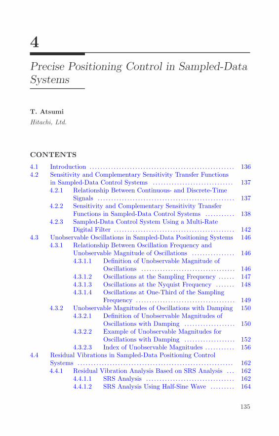
4
Precise Positioning Control in Sampled-DataSystems
T. Atsumi
Hitachi, Ltd.
CONTENTS
4.1 Introduction . . . . . . . . . . . . . . . . . . . . . . . . . . . . . . . . . . . . . . . . . . . . . . . . . . . . . . 1364.2 Sensitivity and Complementary Sensitivity Transfer Functions
in Sampled-Data Control Systems . . . . . . . . . . . . . . . . . . . . . . . . . . . . . . 1374.2.1 Relationship Between Continuous- and Discrete-Time
Signals . . . . . . . . . . . . . . . . . . . . . . . . . . . . . . . . . . . . . . . . . . . . . . . . . . . 1374.2.2 Sensitivity and Complementary Sensitivity Transfer
Functions in Sampled-Data Control Systems . . . . . . . . . . . 1384.2.3 Sampled-Data Control System Using a Multi-Rate
Digital Filter . . . . . . . . . . . . . . . . . . . . . . . . . . . . . . . . . . . . . . . . . . . . . 1424.3 Unobservable Oscillations in Sampled-Data Positioning Systems 146
4.3.1 Relationship Between Oscillation Frequency andUnobservable Magnitude of Oscillations . . . . . . . . . . . . . . . . 1464.3.1.1 Definition of Unobservable Magnitude of
Oscillations . . . . . . . . . . . . . . . . . . . . . . . . . . . . . . . . . . . 1464.3.1.2 Oscillations at the Sampling Frequency . . . . . . 1474.3.1.3 Oscillations at the Nyquist Frequency . . . . . . . 1484.3.1.4 Oscillations at One-Third of the Sampling
Frequency . . . . . . . . . . . . . . . . . . . . . . . . . . . . . . . . . . . . . 1494.3.2 Unobservable Magnitudes of Oscillations with Damping 150
4.3.2.1 Definition of Unobservable Magnitudes ofOscillations with Damping . . . . . . . . . . . . . . . . . . . 150
4.3.2.2 Example of Unobservable Magnitudes forOscillations with Damping . . . . . . . . . . . . . . . . . . . 152
4.3.2.3 Index of Unobservable Magnitudes . . . . . . . . . . . 1564.4 Residual Vibrations in Sampled-Data Positioning Control
Systems . . . . . . . . . . . . . . . . . . . . . . . . . . . . . . . . . . . . . . . . . . . . . . . . . . . . . . . . . . 1624.4.1 Residual Vibration Analysis Based on SRS Analysis . . . 162
4.4.1.1 SRS Analysis . . . . . . . . . . . . . . . . . . . . . . . . . . . . . . . . . 1624.4.1.2 SRS Analysis Using Half-Sine Wave . . . . . . . . . 164
135

136 Advances in High-Performance Motion Control of Mechatronic Systems
4.4.1.3 SRS Analysis Using Polynomial Wave . . . . . . . 1664.4.1.4 Comparison between SRS and DFT . . . . . . . . . 168
4.5 Hard Disk Drive Example . . . . . . . . . . . . . . . . . . . . . . . . . . . . . . . . . . . . . . . . 1754.5.1 Head-Positioning Control System . . . . . . . . . . . . . . . . . . . . . . . 175
4.5.1.1 Controlled Object . . . . . . . . . . . . . . . . . . . . . . . . . . . . 1764.5.2 Sensitivity and Complementary Sensitivity Transfer
Functions . . . . . . . . . . . . . . . . . . . . . . . . . . . . . . . . . . . . . . . . . . . . . . . . 1774.5.2.1 Design of Control System . . . . . . . . . . . . . . . . . . . . 1784.5.2.2 Simulation and Experiment . . . . . . . . . . . . . . . . . . 180
4.5.3 Unobservable Oscillations . . . . . . . . . . . . . . . . . . . . . . . . . . . . . . . 1874.5.4 Residual Vibrations . . . . . . . . . . . . . . . . . . . . . . . . . . . . . . . . . . . . . . 188
4.5.4.1 Feedback Control System . . . . . . . . . . . . . . . . . . . . 1894.5.4.2 Feedforward Control System . . . . . . . . . . . . . . . . . 1914.5.4.3 SRS Analysis . . . . . . . . . . . . . . . . . . . . . . . . . . . . . . . . . 1924.5.4.4 Simulation and Experimental Results . . . . . . . . 193
4.1 Introduction
The wide availability of inexpensive microprocessors has made sampled-datacontrol systems very popular for positioning control in mechatronic products.As a result, the sampled-data control system could be assumed to be the stan-dard control system in these engineering systems. The sampled-data controlsystem is a hybrid system which includes continuous-time and discrete-timesignals, implying that the controlled variable is measured only at specific in-stants. As such, the intersample behavior can degrade the performance andreliability of these systems. For example, in the head-positioning control sys-tem of Hard Disk Drives (HDDs), the unobservable head-position may causedestruction of user data stored in HDDs.
There are essentially three different approaches to design controllers forsampled-data control systems. The first approach is continuous-time controlsystem design, where discretization errors cannot be avoided and may degradethe control performance and/or stability of the control system. The secondapproach is discrete-time control system design, which can compensate for thediscretization errors but does not account for the behaviors of the continuous-time signal between samples. The last approach is sampled-data control systemdesign, which can compensate for the discretization errors by considering theintersampling behaviors of the continuous-time signals. Nevertheless, the firstand second approaches are more widely employed because of their ease of use,while the last approach is not generally used in the positioning control systemof mechatronic products since it is generally more difficult to understand andapply.
To address these concerns, we propose the following calculation methodsfor

Precise Positioning Control in Sampled-Data Systems 137
1. sensitivity and complementary sensitivity transfer functions insampled-data control systems [1];
2. unobservable oscillations in sampled-data positioning systems [2];and
3. residual vibrations in sampled-data positioning control systems [3].
4.2 Sensitivity and Complementary Sensitivity TransferFunctions in Sampled-Data Control Systems
A main reason why sampled-data control system design is not popular is thedifficulty in handling the corresponding frequency responses, since sampled-data control systems are not Linear Time-Invariant (LTI) systems. To over-come these problems, a method based on frequency responses for the calcu-lation of the sensitivity and complementary sensitivity transfer functions of asampled-data control system is shown. In this method, the gains of the sen-sitivity and complementary sensitivity transfer functions can be evaluated bythe maximum displacement of the control variable. As such, infinity norms ofsignals can be used to define the gain of the sensitivity transfer functions fordisturbance suppression in sampled-data positioning control systems.
4.2.1 Relationship Between Continuous- and Discrete-TimeSignals
In this section, the relationship between a continuous- and discrete-time signalis defined. For simplicity but without loss of generality, a sinusoidal wave x0(t)is defined as
x0(t) = ejω0t. (4.1)
The discrete-time signal xd(n) corresponding to the signal after sampling x0(t)at a sampling time Ts can be given as
xd(n) = x0(nTs)
= ejω0nTs . (4.2)
The continuous-time signal xc(t) which is created from xd(n) can be given as
xc(t) =
∞∑l=−∞
δ(t− lTs)ejω0t
=1
Ts
∞∑l=−∞
ej(ω0+ωsl)t, (4.3)

138 Advances in High-Performance Motion Control of Mechatronic Systems
where δ is the Dirac delta function. From (4.2) and (4.3), it can be observedthat the discrete-time signal caused by a single complex sinusoid can be rep-resented by a single frequency, while the continuous-time signal caused by thediscrete-time signal consists of multiple frequencies.
4.2.2 Sensitivity and Complementary Sensitivity TransferFunctions in Sampled-Data Control Systems
The block diagram of a sampled-data control system is shown in Figure 4.1.In this figure, S is a sampler, C is a digital controller, H is a hold, and Pc is acontinuous-time plant. r is a reference signal, ud is an output signal from C,uc is an output signal from H, dc is a disturbance signal in continuous time,yc0 is an output signal from Pc, yd0 is a sampled signal of yc0, yc is a controlledvariable in continuous time, and yd is a controlled variable in discrete time. Inthis example, the sampling time Ts is in seconds and the sampling frequencyis ωs =
2πTs
rad/s.To avoid complex calculations involving matrix algebra, we use frequency
responses to analyze the sampled-data control system [1]. The transfer char-acteristics from ud to yd at ω0 is the controlled object in the discrete-timesystem denoted as Pd(jω0), and is given as
Pd(jω0) =1
Ts
∞∑k=−∞
H(jω0 + jωsk)Pc(jω0 + jωsk). (4.4)
In this case, the disturbance signal dc(t, ω0) is a single complex sinusoid andis given as
dc(t, ω0) = ejω0t. (4.5)
At steady-state with dc, ud can be given by
ud(n) =−C(ejω0Ts)
1 + Pd(jω0)C(ejω0Ts)ejω0Tsn, (4.6)
and uc(t) is given by
uc(t) =−C(ejω0Ts)
1 + Pd(jω0)C(ejω0Ts)
1
Ts
∞∑l=−∞
H(jω0 + jωsl)ej(ω0+ωsl)t. (4.7)
yc0(t) is given by
yc0(t) =
∞∑l=−∞
Γ(ω0, l)ej(ω0+ωsl)t, (4.8)
where
Γ(ω, l) = − 1
Ts
C(ejωTs)H(jω + jωsl)Pc(jω + jωsl)
1 + Pd(jω)C(ejωTs ), ∀l ∈ Z. (4.9)

Precise Positioning Control in Sampled-Data Systems 139
By summing dc and yc0, yc(t) can be obtained as
yc(t) = ejω0t +
∞∑l=−∞
Γ(ω0, l)ej(ω0+ωsl)t. (4.10)
yd0(n) is given by
yd0(n) = yc0(nTs)
=∞∑
l=−∞Γ(ω0, l)e
j(ω0Ts+2πl)n
=
( ∞∑l=−∞
Γ(ω0, l)
)ejω0Tsn
=−Pd(jω0)C(e
jω0Ts)
1 + Pd(jω0)C(ejω0Ts)ejω0Tsn, (4.11)
and yd(n) is given by
yd(n) = yc(nTs) = ejω0Tsn +
∞∑l=−∞
Γ(ω0, l)ej(ω0Ts+2πl)n
=
(1 +
∞∑l=−∞
Γ(ω0, l)
)ejω0Tsn
=1
1 + Pd(jω0)C(ejω0Ts)ejω0Tsn. (4.12)
yc0 and yc consist of multiple frequencies as shown in (4.8) and (4.10),respectively. This means that the transfer characteristics from dc to yc0 andfrom dc to yc are not LTI systems. As such, LTI transfer functions cannot bedefined for sampled-data control systems, and the stability of sampled-datacontrol systems should be designed using discrete-time control techniques tomake the system stable at the sampled-data points.
In a positioning control system, the performance of the control systemcan be evaluated by the maximum displacement of the control variable. Assuch, infinity norms of the signals can be used for defining the gains of thesensitivity and complementary sensitivity transfer functions for performanceevaluation in sampled-data positioning control systems.
Using dc(t, ω0) = ejω0t and yc0 which are shown in Figure 4.1 and (4.8), themagnitude response of the complementary sensitivity transfer function |Tsd|

140 Advances in High-Performance Motion Control of Mechatronic Systems
in a sampled-data control system at ω0 is given by
|Tsd(jω0)| =||yc0(t)||∞
||dc(t, ω0)||∞= sup
t|yc0(t)|
=
∞∑l=−∞
|Γ(ω0, l)| . (4.13)
|Tsd| is a periodic function as indicated by (4.13), and is given as
|Tsd(jω0)| = |Tsd(jω0 + jω0l)|, ∀l ∈ Z. (4.14)
From (4.11), the complementary sensitivity transfer function Td of thediscrete-time system can be given as
Td(jω0) =Pd(jω0)C(e
jω0Ts)
1 + Pd(jω0)C(ejω0Ts)
= −∞∑
l=−∞Γ(ω0, l). (4.15)
The difference between |Td| and |Tsd| is |TΔ|, and can be given as
|TΔ(jω0)| = |Tsd(jω0)| − |Td(jω0)|
=
∞∑l=−∞
|Γ(ω0, l)| −∣∣∣∣∣
∞∑l=−∞
Γ(ω0, l)
∣∣∣∣∣ . (4.16)
|TΔ(jω0)| indicates the ratio between the amplitude of the intersampling vi-brations and the amplitude of the sampled-point vibration caused by the noiseat ω0. As such, the control system must make |TΔ(jω0)| small when the controlsystem has a large noise signal at ω0.
Similarly, using dc(t, ω0) = ejω0t and yc which are shown in Figure 4.1and (4.10), the magnitude response of the sensitivity transfer function in asampled-data control system at ω0 is given by
|Ssd(jω0)| =||yc(t)||∞
||dc(t, ω0)||∞= sup
t|yc(t)|
= |1 + Γ(ω0, 0)|+∞∑
l=−∞, �=0
|Γ(ω0, l)|. (4.17)
|Ssd| is not a periodic function like that of discrete-time systems and |Tsd|,

Precise Positioning Control in Sampled-Data Systems 141
as can be seen from (4.17). It is also indicated in (4.17) that the control systemmust satisfy
|Γ(ω0, 0)| >∞∑
l=−∞, �=0
|Γ(ω0, l)|, (4.18)
in order to make|Ssd(jω0)| < 1. (4.19)
In other words, when the control system achieves (4.19), the control systemwill have
|Ssd(jω0 + jωsl)| > 1, ∀l �= 0, (4.20)
because |Γ(ω0, l)| <∑∞k=−∞, �=l |Γ(ω0, k)|. In particular, when |Ssd(jω0)| � 0,
|Ssd(jω0 + jωsl)| � 2, ∀l �= 0. (4.21)
It should be noted that (4.18) is not a sufficient condition for (4.19).From (4.12), the sensitivity transfer function Sd of the discrete-time system
can be given as
Sd(jω0) =1
1 + Pd(jω0)C(ejω0Ts)
= 1 +∞∑
l=−∞Γ(ω0, l). (4.22)
The difference between |Sd| and |Ssd| can now be given as
|SΔ(jω0)| = |Ssd(jω0)| − |Sd(jω0)|
= |1 + Γ(ω0, 0)|+∞∑
l=−∞, �=0
|Γ(ω0, l)| −∣∣∣∣∣1 +
∞∑l=−∞
Γ(ω0, l)
∣∣∣∣∣ .
(4.23)
|SΔ(jω0)| indicates the ratio between the amplitude of the intersampling vi-brations and the amplitude of the sampled-point vibration caused by the dis-turbance at ω0. Therefore, the control system must make |SΔ(jω0)| smallwhen the control system has a large disturbance at ω0.
From (4.13) and (4.17), the relationship between |Ssd| and |Tsd| can begiven as
|Ssd(jω0)| = |Tsd(jω0)| − |Γ(ω0, 0)|+ |1 + Γ(ω0, 0)|. (4.24)
|Tsd(jω0)| − |Γ(ω0, 0)| shows that the effects of the aliasing frequencies ofω0 on |Tsd(jω0)|. Therefore, the control system needs to make the effects ofthe aliasing frequencies of ω0 on |Tsd(jω0)| small in order to make |Ssd(jω0)|small. Besides, it is also shown by (4.24) that when |Ssd(jω0)| � 0, |Tsd(jω0)|becomes approximately 1.
With these notions, the results for the sensitivity and complementary sen-sitivity transfer functions of a sampled-data control system can be summarizedas follows:

142 Advances in High-Performance Motion Control of Mechatronic Systems
• The relationship between |Ssd| and |Tsd| are given by (4.24). This impliesthat the control system needs to make the effects of the aliasing frequenciesof ω0 on |Tsd(jω0)| small in order to make |Ssd(jω0)| small;
• |Tsd| is a periodic function similar to that of discrete-time systems, but |Ssd|is not a periodic function;
• When the sampled-data control system achieves |Ssd(jω0)| < 1, |Ssd(jω0 +jωsl)| > 1 for all l �= 0;
• When |Ssd(jω0)| � 0, |Ssd(jω0+ jωsl)| � 2 ∀l �= 0 and |Tsd(jω0+ jωsl)| � 1for all l;
• The control system must make |TΔ(jω0)| small when the control system hasa large noise signal at ω0; and
• The control system must make |SΔ(jω0)| small when the control system hasa large disturbance at ω0;
4.2.3 Sampled-Data Control System Using a Multi-RateDigital Filter
In sampled-data control systems, multi-rate filters are often used to improvethe control performance. In this section, the focus is on sampled-data controlsystems using multi-rate filters realized with multi-rate holds and interpolatorsso that the frequency responses of the multi-rate system can be defined. Theblock diagram of a sampled-data control system with a multi-rate digital filteris shown in Figure 4.2. In this figure, Ip is an interpolator, Fm is a multi-ratedigital filter, and Hm is a multi-rate hold. The multi-rate number is definedas m.
The transfer characteristics from ud to yd at ω0 is the controlled object inthe discrete-time system which includes the multi-rate filter. This is denotedas Pdm(jω0), and is given as
Pdm(jω0) =1
Ts
∞∑k=−∞
W (jω0 + jωsk)Pc(jω0 + jωsk), (4.25)
whereW (jω) = Ip(e
jωTsm )Fm(e
jωTsm )Hm(jω). (4.26)
yc0(t) consists of multiple frequencies and is given by
yc0(t) =∞∑
l=−∞Γm(ω0, l)e
j(ω0+ωsl)t, (4.27)
where
Γm(ω, l) = − 1
Ts
C(ejωTs)W (jω + jωsl)Pc(jω + jωsl)
1 + Pdm(jω)C(ejωTs ), ∀l ∈ Z. (4.28)
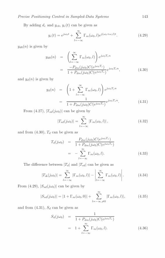
Precise Positioning Control in Sampled-Data Systems 143
By adding dc and yc0, yc(t) can be given as
yc(t) = ejω0t +
∞∑l=−∞
Γm(ω0, l)ej(ω0+ωsl)t. (4.29)
yd0(n) is given by
yd0(n) =
( ∞∑l=−∞
Γm(ω0, l)
)ejω0Tsn
=−Pdm(jω0)C(e
jω0Ts)
1 + Pdm(jω0)C(ejω0Ts)ejω0Tsn, (4.30)
and yd(n) is given by
yd(n) =
(1 +
∞∑l=−∞
Γm(ω0, l)
)ejω0Tsn
=1
1 + Pdm(jω0)C(ejω0Ts)ejω0Tsn. (4.31)
From (4.27), |Tsd(jω0)| can be given by
|Tsd(jω0)| =∞∑
l=−∞|Γm(ω0, l)| , (4.32)
and from (4.30), Td can be given as
Td(jω0) =Pdm(jω0)C(e
jω0Ts)
1 + Pdm(jω0)C(ejω0Ts)
= −∞∑
l=−∞Γm(ω0, l). (4.33)
The difference between |Td| and |Tsd| can be given as
|TΔ(jω0)| =∞∑
l=−∞|Γm(ω0, l)| −
∣∣∣∣∣∞∑
l=−∞Γm(ω0, l)
∣∣∣∣∣ . (4.34)
From (4.29), |Ssd(jω0)| can be given by
|Ssd(jω0)| = |1 + Γm(ω0, 0)|+∞∑
l=−∞, �=0
|Γm(ω0, l)|, (4.35)
and from (4.31), Sd can be given as
Sd(jω0) =1
1 + Pdm(jω0)C(ejω0Ts)
= 1 +
∞∑l=−∞
Γm(ω0, l). (4.36)

144 Advances in High-Performance Motion Control of Mechatronic Systems
The difference between |Sd| and |Ssd| can be given as
|SΔ(jω0)| = |1 + Γm(ω0, 0)|+∞∑
l=−∞, �=0
|Γm(ω0, l)| −∣∣∣∣∣1 +
∞∑l=−∞
Γm(ω0, l)
∣∣∣∣∣ .
(4.37)From (4.32) and (4.35), the relationship between |Ssd| and |Tsd| can be
given as
|Ssd(jω0)| = |Tsd(jω0)| − |Γm(ω0, 0)|+ |1 + Γm(ω0, 0)|. (4.38)
The above-mentioned results show that the characteristics of the sensi-tivity and complementary sensitivity transfer functions of the sampled-datacontrol system with a multi-rate filter are similar to that of the sampled-datacontrol system without a multi-rate filter. As such, the results for a multi-ratesampled-data control system are summarized as follows:
• The relationship between |Ssd| and |Tsd| are given by (4.38);
• |Tsd| is a periodic function similar to that of discrete-time systems, but |Ssd|is not a periodic function;
• When the sampled-data control system achieves |Ssd(jω0)| < 1, |Ssd(jω0 +jωsl)| > 1 for all l �= 0;
• When |Ssd(jω0)| � 0, |Ssd(jω0+ jωsl)| � 2 ∀l �= 0 and |Tsd(jω0+ jωsl)| � 1for all l;
• The control system must make |TΔ(jω0)| small when the control system hasa large noise signal at ω0; and
• The control system must make |SΔ(jω0)| small when the control system hasa large disturbance at ω0.

Precise Positioning Control in Sampled-Data Systems 145
S
C
H Pc
r
ydyc0uc
ud
dc
yc+
−
+
+
S
yd0
FIGURE 4.1Block diagram of a sampled-data control system.
SHm Pc
r
ydyc0uc
dc
yc+
−
+
+
S
yd0
CudIpFm
FIGURE 4.2Block diagram of a sampled-data control system with a multi-rate filter.

146 Advances in High-Performance Motion Control of Mechatronic Systems
4.3 Unobservable Oscillations in Sampled-Data Posi-tioning Systems
The term unobservable oscillation refers to the movement of a controlled posi-tion variable that occurs between samples, which usually arises from mechan-ical vibrations. The degree of unobservability depends on the relationship be-tween the sampling frequency and the oscillation frequency. The relationshipbetween the oscillation frequency and the sampling frequency is shown usingan index of unobservable magnitude of oscillations based on its Root-Mean-Square (RMS) amplitude. By using this index, the effects of the unobservableoscillations caused by mechanical resonances can be estimated.
4.3.1 Relationship Between Oscillation Frequency and Un-observable Magnitude of Oscillations
The performance of a positioning control system can be evaluated by lookingat the maximum displacement of the controlled variable. In the sampled-datapositioning control system shown in Figure 4.1, the maximum displacementfrom yd is observed by the control system. However, the actual position isyc. Therefore, the sampled-data control system has an unobservable magni-tude which is the difference between the maximum displacement of yc and themaximum displacement of yd. When the unobservable magnitude is large, theperformance and reliability of the mechatronic products may degrade. Conse-quently, the control system must ensure that the magnitude of the unobserv-able signal is small enough for the device to operate with good performancereliably.
4.3.1.1 Definition of Unobservable Magnitude of Oscillations
In this section, the effects of the sampler are studied where the position signalyc is a sinusoid given by
yc(t) = sin (ωtt) , (4.39)
and ωt is the oscillation frequency in rad/s. The discrete-time signal yd cor-responds to the signal after sampling yc with sampling time τ and is givenas
yd[n,Δs] = yc(τ(n+Δs))
= sin (ωtτ(n +Δs)) , (4.40)
where n is the sample number and Δs is the timing of the sampling (0 ≤ Δs <1) within one sampling period. The unobservable magnitude yu is defined as
yu[Δs] = max(|yum[Δs]|, |yup[Δs]|), (4.41)
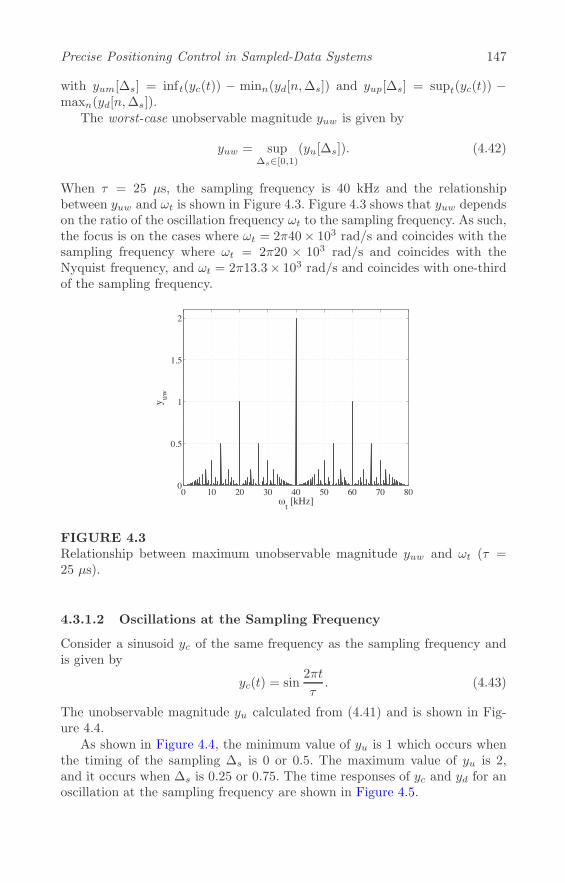
Precise Positioning Control in Sampled-Data Systems 147
with yum[Δs] = inft(yc(t)) − minn(yd[n,Δs]) and yup[Δs] = supt(yc(t)) −maxn(yd[n,Δs]).
The worst-case unobservable magnitude yuw is given by
yuw = supΔs∈[0,1)
(yu[Δs]). (4.42)
When τ = 25 μs, the sampling frequency is 40 kHz and the relationshipbetween yuw and ωt is shown in Figure 4.3. Figure 4.3 shows that yuw dependson the ratio of the oscillation frequency ωt to the sampling frequency. As such,the focus is on the cases where ωt = 2π40× 103 rad/s and coincides with thesampling frequency where ωt = 2π20 × 103 rad/s and coincides with theNyquist frequency, and ωt = 2π13.3× 10³ rad/s and coincides with one-thirdof the sampling frequency.
0 10 20 30 40 50 60 70 800
0.5
1
1.5
2
ωt [kHz]
y uw
FIGURE 4.3Relationship between maximum unobservable magnitude yuw and ωt (τ =25 μs).
4.3.1.2 Oscillations at the Sampling Frequency
Consider a sinusoid yc of the same frequency as the sampling frequency andis given by
yc(t) = sin2πt
τ. (4.43)
The unobservable magnitude yu calculated from (4.41) and is shown in Fig-ure 4.4.
As shown in Figure 4.4, the minimum value of yu is 1 which occurs whenthe timing of the sampling Δs is 0 or 0.5. The maximum value of yu is 2,and it occurs when Δs is 0.25 or 0.75. The time responses of yc and yd for anoscillation at the sampling frequency are shown in Figure 4.5.
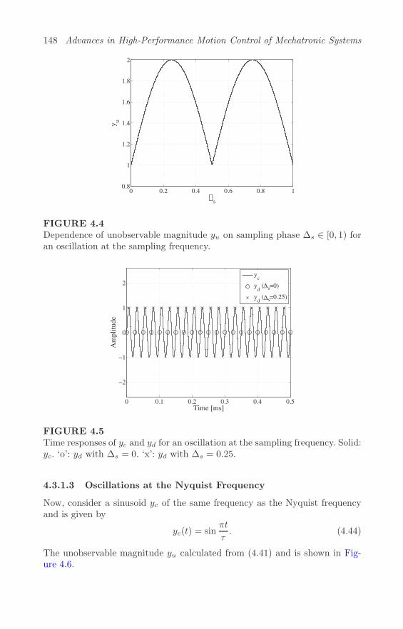
148 Advances in High-Performance Motion Control of Mechatronic Systems
0 0.2 0.4 0.6 0.8 10.8
1
1.2
1.4
1.6
1.8
2
s
y u
FIGURE 4.4Dependence of unobservable magnitude yu on sampling phase Δs ∈ [0, 1) foran oscillation at the sampling frequency.
0 0.1 0.2 0.3 0.4 0.5
−2
−1
0
1
2
Time [ms]
Am
plitu
de
ycyd ( s=0)
yd ( s=0.25)Δ
Δ
FIGURE 4.5Time responses of yc and yd for an oscillation at the sampling frequency. Solid:yc. ‘o’: yd with Δs = 0. ‘x’: yd with Δs = 0.25.
4.3.1.3 Oscillations at the Nyquist Frequency
Now, consider a sinusoid yc of the same frequency as the Nyquist frequencyand is given by
yc(t) = sinπt
τ. (4.44)
The unobservable magnitude yu calculated from (4.41) and is shown in Fig-ure 4.6.

Precise Positioning Control in Sampled-Data Systems 149
0 0.2 0.4 0.6 0.8 10
0.2
0.4
0.6
0.8
1
s
y u
Δ
FIGURE 4.6Unobservable magnitude for an oscillation at the Nyquist frequency.
As shown in Figure 4.6, the minimum unobservable magnitude yu = 0occurs when the sampling phase Δs = 0.5. The maximum unobservable mag-nitude yu = 1 occurs when Δs = 0. The time responses of yc and yd for anoscillation at the Nyquist frequency are shown in Figure 4.7.
0 0.1 0.2 0.3 0.4 0.5
−2
−1
0
1
2
Time [ms]
Am
plitu
de
ycyd ( s=0.5)
yd ( s=0)Δ
Δ
FIGURE 4.7Time responses of yc and yd for an oscillation at the Nyquist frequency. Solid:yc. ‘o’: yd with Δs = 0.5. ‘x’: yd with Δs = 0.

150 Advances in High-Performance Motion Control of Mechatronic Systems
4.3.1.4 Oscillations at One-Third of the Sampling Frequency
The third case considered is a sinusoid yc of frequency that is one-third of thesampling frequency, and is given by
yc(t) = sin2πt
3τ. (4.45)
The unobservable magnitude yu calculated from (4.41) is shown in Figure 4.8.
0 0.2 0.4 0.6 0.8 10.1
0.15
0.2
0.25
0.3
0.35
0.4
0.45
0.5
s
y u
Δ
FIGURE 4.8Unobservable magnitude for an oscillation at one-third of the sampling fre-quency.
As shown in Figure 4.8, the minimum unobservable magnitude yu = 0.134occurs when the timing of the sampling Δs = 0 or Δs = 0.5, and the maximumunobservable magnitude yu = 0.5 occurs when Δs = 0.25 or Δs = 0.75. Thetime responses of yc and yd for an oscillation at one-third of the samplingfrequency are shown in Figure 4.9.
4.3.2 Unobservable Magnitudes of Oscillations with Damp-ing
In this section, we consider and study the effects of unobservable magnitudesof oscillations with positive damping. This is more practical since most os-cillations arising from mechanical vibrations are passive in nature and decaywith time.
4.3.2.1 Definition of Unobservable Magnitudes of Oscillations withDamping
For a positioning control system in mechatronic products, many of the oscil-lations in the position signal are caused by damped mechanical resonances.

Precise Positioning Control in Sampled-Data Systems 151
0 0.1 0.2 0.3 0.4 0.5
−2
−1
0
1
2
Time [ms]
Am
plitu
de
ycyd ( s=0)
yd ( s=0.25)
Δ
Δ
Δ
FIGURE 4.9Time responses of yc and yd for an oscillation at one-third of the samplingfrequency. Solid: yc. ‘o’: yd with Δs = 0. ‘x’: yd with Δs = 0.75.
As such, the oscillation signal yc and measurement data yd are redefined as
yc(t) = e−ζωnt sin (ωdt), (4.46)
and
yd[n,Δs] = yc(τ(n+Δs))
= e−ζωnτ(n+Δs) sin (ωdτ(n +Δs)), (4.47)
where ωn and ζ are the natural frequency and damping ratio of the resonantmode, respectively, and ωd = ωn
√(1− ζ2) is the damped natural frequency.
In general, a positioning control system must estimate the maximum dis-placement of the control variable from a finite number of samples of the posi-tion signal. For example, the head-positioning control system of an HDD mustdetermine the data writability by comparing a finite number of samples of po-sition signal against the write-inhibit condition. Therefore, the unobservablemagnitude has to be considered, which is the difference between the maximumdisplacement of yc and the maximum displacement of yd for a finite number ofsamples. The unobservable magnitude yu for a finite number of samples canbe redefined as
yu[Δs] =
⎧⎪⎪⎪⎪⎨⎪⎪⎪⎪⎩
0 : yup[Δs] ≤ 0, yum[Δs] ≥ 0|yup[Δs]| : yup[Δs] > 0, yum[Δs] ≥ 0|yum[Δs]| : yup[Δs] ≤ 0, yum[Δs] < 0|yup[Δs]| : yup[Δs] ≥ −yum[Δs] > 0|yum[Δs]| : −yum[Δs] > yup[Δs] > 0
, (4.48)
where yum[Δs] = inft∈[Nsτ,∞)(yc(t)) − minn∈[1,Ns](yd[n,Δs]) and yup[Δs] =supt∈[Nsτ,∞)(yc(t))−maxn∈[1,Ns](yd[n,Δs]), and Ns is the sample number forthe judgment of the maximum displacement. An example of the time responsesof yc and yd with Ns = 5 is shown in Figure 4.10. In this case, yu is equal to|yum| because yup ≤ 0 and yum < 0.
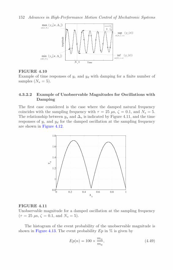
152 Advances in High-Performance Motion Control of Mechatronic Systems
FIGURE 4.10Example of time responses of yc and yd with damping for a finite number ofsamples (Ns = 5).
4.3.2.2 Example of Unobservable Magnitudes for Oscillations withDamping
The first case considered is the case where the damped natural frequencycoincides with the sampling frequency with τ = 25 μs, ζ = 0.1, and Ns = 5.The relationship between yu and Δs is indicated by Figure 4.11, and the timeresponses of yc and yd for the damped oscillation at the sampling frequencyare shown in Figure 4.12.
0 0.2 0.4 0.6 0.8 10.8
1
1.2
1.4
1.6
1.8
s
y u
Δ
FIGURE 4.11Unobservable magnitude for a damped oscillation at the sampling frequency(τ = 25 μs, ζ = 0.1, and Ns = 5).
The histogram of the event probability of the unobservable magnitude isshown in Figure 4.13. The event probability Ep in % is given by
Ep(n) = 100× mn
ma, (4.49)

Precise Positioning Control in Sampled-Data Systems 153
0 0.1 0.2 0.3 0.4 0.5−2
−1.5
−1
−0.5
0
0.5
1
1.5
2
Time [ms]
Am
plitu
de
ycyd ( s=0)
yd ( s=0.25)Δ
Δ
FIGURE 4.12Time responses of yc and yd for a damped oscillation at the sampling frequency(τ = 25 μs, ζ = 0.1, and Ns = 5). Solid: yc. ‘o’: yd with Δs = 0. ‘x’: yd withΔs = 0.25.
where mn counts the number of observations that fall into
0.1(n− 1) ≤ yu < 0.1n, (4.50)
and ma counts the total number of observations. In this case, most of themagnitudes are more than 140% of the amplitude.
0 50 100 150 2000
10
20
30
40
50
60
70
Even
t pro
babi
lity
[%]
Unobservable amplitudes [% of amplitude]
FIGURE 4.13Histogram of event probability of unobservable magnitude for a damped os-cillation at the sampling frequency (τ = 25 μs, ζ = 0.1, and Ns = 5).
The second case considered is the case where the damped natural frequency

154 Advances in High-Performance Motion Control of Mechatronic Systems
coincides with the Nyquist frequency with τ = 25 μs, ζ = 0.1, and Ns = 5.The relationship between yu and Δs is indicated by Figure 4.14, and the timeresponses of yc and yd for the damped oscillation at the Nyquist frequencyare shown in Figure 4.15.
0 0.2 0.4 0.6 0.8 10
0.2
0.4
0.6
0.8
1
s
y u
Δ
FIGURE 4.14Unobservable magnitude for a damped oscillation at the Nyquist frequency (τ= 25 μs, ζ = 0.1, and Ns = 5).
0 0.1 0.2 0.3 0.4 0.5−2
−1.5
−1
−0.5
0
0.5
1
1.5
2
Time [ms]
Am
plitu
de
ycyd (∆
(∆s=0.5)
yd s=0)
FIGURE 4.15Time responses of yc and yd for a damped oscillation at the Nyquist frequency(τ = 25 μs, ζ = 0.1, and Ns = 5). Solid: yc. ‘o’: yd with Δs = 0.5. ‘x’: yd withΔs = 0.
The histogram of the event probability of the unobservable magnitudes is
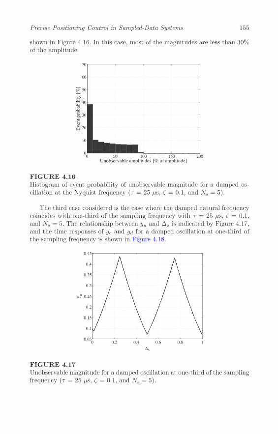
Precise Positioning Control in Sampled-Data Systems 155
shown in Figure 4.16. In this case, most of the magnitudes are less than 30%of the amplitude.
0 50 100 150 2000
10
20
30
40
50
60
70
Even
t pro
babi
lity
[%]
Unobservable amplitudes [% of amplitude]
FIGURE 4.16Histogram of event probability of unobservable magnitude for a damped os-cillation at the Nyquist frequency (τ = 25 μs, ζ = 0.1, and Ns = 5).
The third case considered is the case where the damped natural frequencycoincides with one-third of the sampling frequency with τ = 25 μs, ζ = 0.1,and Ns = 5. The relationship between yu and Δs is indicated by Figure 4.17,and the time responses of yc and yd for a damped oscillation at one-third ofthe sampling frequency is shown in Figure 4.18.
0 0.2 0.4 0.6 0.8 10.05
0.1
0.15
0.2
0.25
0.3
0.35
0.4
0.45
s
y u
Δ
FIGURE 4.17Unobservable magnitude for a damped oscillation at one-third of the samplingfrequency (τ = 25 μs, ζ = 0.1, and Ns = 5).

156 Advances in High-Performance Motion Control of Mechatronic Systems
0 0.1 0.2 0.3 0.4 0.5−2
−1.5
−1
−0.5
0
0.5
1
1.5
2
Time [ms]
Am
plitu
de
ycyd ( s=0)
yd ( s=0.25)Δ
Δ
FIGURE 4.18Time responses of yc and yd for a damped oscillation at one-third of thesampling frequency (τ = 25 μs, ζ = 0.1, and Ns = 5). Solid: yc. ‘o’: yd withΔs = 0. ‘x’: yd with Δs = 0.25.
The histogram of the event probability of the unobservable magnitude isshown in Figure 4.19. In this case, most of the magnitudes are less than 30%of the amplitude.
0 50 100 150 2000
10
20
30
40
50
60
70
Even
t pro
babi
lity
[%]
Unobservable amplitudes [% of amplitude]
FIGURE 4.19Histogram of event probability of unobservable magnitude for a damped os-cillation at one-third of the sampling frequency (τ = 25 μs, ζ = 0.1, andNs = 5).

Precise Positioning Control in Sampled-Data Systems 157
4.3.2.3 Index of Unobservable Magnitudes
The worst-case unobservable magnitude yuw for a finite number of samples isgiven by
yuw = supΔs∈[0,1)
(yu[Δs]). (4.51)
The worst-case unobservable magnitude yuw with τ = 25 μs and ζ = 0 isshown in Figure 4.20. Figure 4.21 shows yuw with τ = 25 μs and ζ = 0.01. Itcan be seen that the areas where yuw is large become wider under finite samplenumber, especially around the sampling frequency. The widths of the peaksof yuw become narrower as Ns increases. Besides, it can also be seen that yuwbecomes smaller as ζ increases. This effect becomes larger as ωd increases.
0 10 20 30 40 50 60 70 800
0.5
1
1.5
2
ωd [kHz]
y uw
5 sample10 sample20 sample
FIGURE 4.20Relationship between yuw and ωd (τ = 25 μs and ζ = 0). Dashed: Ns = 5.Dashed-dot: Ns = 10. Solid: Ns = 20.
The worst-case unobservable magnitude and its event probability dependon the relationship between the oscillation frequency and the sampling fre-quency. This means that the index of unobservable magnitude that includesthe worst-case value and its event probability have to be defined. For example,yuw at the sampling frequency is twice that at the Nyquist frequency as shownin Figure 4.3. However, it can be seen from Figures 4.13 and 4.16 that the riskof degradation of performance and reliability caused by the oscillation at thesampling frequency is much higher than that caused by the oscillation at theNyquist frequency.
As such by using the RMS value of yu, the index value of unobservablemagnitude yui which includes the effects of the event probability is proposedto be
yui =
√∫ 1
0
yu[Δs]2dΔs, (4.52)
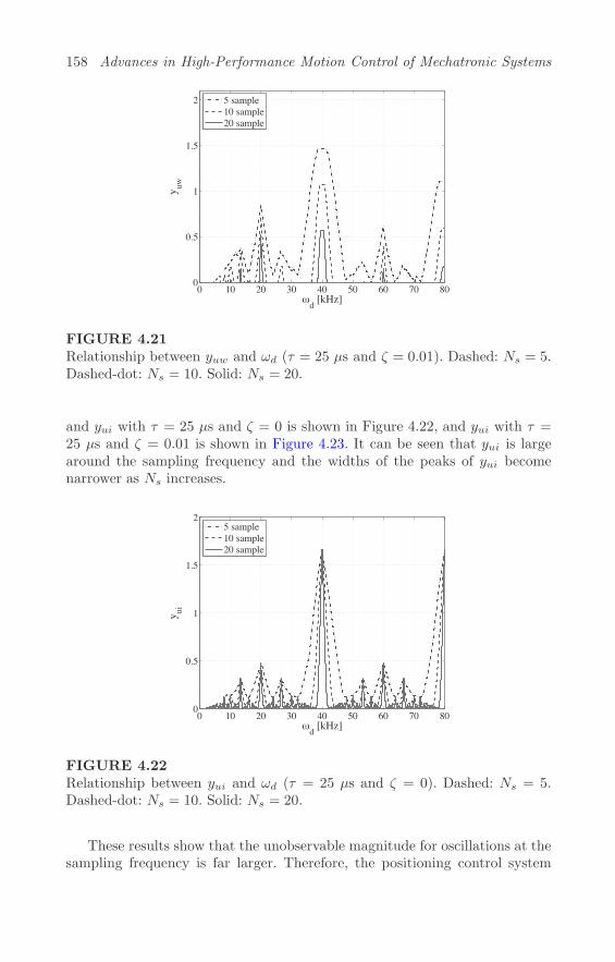
158 Advances in High-Performance Motion Control of Mechatronic Systems
0 10 20 30 40 50 60 70 800
0.5
1
1.5
2
ωd [kHz]
y uw
5 sample10 sample20 sample
FIGURE 4.21Relationship between yuw and ωd (τ = 25 μs and ζ = 0.01). Dashed: Ns = 5.Dashed-dot: Ns = 10. Solid: Ns = 20.
and yui with τ = 25 μs and ζ = 0 is shown in Figure 4.22, and yui with τ =25 μs and ζ = 0.01 is shown in Figure 4.23. It can be seen that yui is largearound the sampling frequency and the widths of the peaks of yui becomenarrower as Ns increases.
0 10 20 30 40 50 60 70 800
0.5
1
1.5
2
ωd [kHz]
y ui
5 sample10 sample20 sample
FIGURE 4.22Relationship between yui and ωd (τ = 25 μs and ζ = 0). Dashed: Ns = 5.Dashed-dot: Ns = 10. Solid: Ns = 20.
These results show that the unobservable magnitude for oscillations at thesampling frequency is far larger. Therefore, the positioning control system
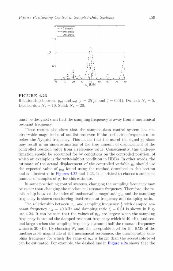
Precise Positioning Control in Sampled-Data Systems 159
0 10 20 30 40 50 60 70 800
0.5
1
1.5
2
ωd [kHz]
y ui
5 sample10 sample20 sample
FIGURE 4.23Relationship between yui and ωd (τ = 25 μs and ζ = 0.01). Dashed: Ns = 5.Dashed-dot: Ns = 10. Solid: Ns = 20.
must be designed such that the sampling frequency is away from a mechanicalresonant frequency.
These results also show that the sampled-data control system has un-observable magnitudes of oscillations even if the oscillation frequencies arebelow the Nyquist frequency. This means that the use of the signal yd alonemay result in an underestimation of the true amount of displacement of thecontrolled position value from a reference value. Consequently, this underes-timation should be accounted for by conditions on the controlled position, ofwhich an example is the write-inhibit condition in HDDs. In other words, theestimate of the actual displacement of the controlled variable yc should usethe expected value of yui found using the method described in this sectionand as illustrated in Figures 4.22 and 4.23. It is critical to choose a sufficientnumber of samples of yd for this estimate.
In some positioning control systems, changing the sampling frequency maybe easier than changing the mechanical resonant frequency. Therefore, the re-lationship between the index of unobservable magnitude yui and the samplingfrequency is shown considering fixed resonant frequency and damping ratio.
The relationship between yui and sampling frequency 1τ with damped res-
onant frequency ωd = 40 kHz and damping ratio ζ = 0.01 is shown in Fig-ure 4.24. It can be seen that the values of yui are largest when the samplingfrequency is around the damped resonant frequency which is 40 kHz, and sec-ond largest when the sampling frequency is around half the resonant frequencywhich is 20 kHz. By choosing Ns and the acceptable level for the RMS of theunobservable magnitude of the mechanical resonance, the unacceptable sam-pling frequency for which the value of yui is larger than the acceptable levelcan be estimated. For example, the dashed line in Figure 4.24 shows that the

160 Advances in High-Performance Motion Control of Mechatronic Systems
sampling frequency should not be set around 13.3 kHz, 20.0 kHz, 40.0 kHz,and 80.0 kHz, when the acceptable level is 0.2 and Ns = 10.
104 1050
0.2
0.5
1
1.5
Sampling frequency [Hz]
yui
5 sample10 sample20 sample
FIGURE 4.24Relationship between yui and the sampling frequency, with ωd = 40 kHz andζ = 0.01. Solid: Ns = 5. Dashed: Ns = 10. Dashed-dot: Ns = 20.
The dependence of yui on the measurement time τ ×Ns for the judgmentof the maximum displacement with ωd = 40 kHz and ζ = 0.01 is shown inFigure 4.25. It can be seen that yui becomes smaller with increasing τ×Ns, andthe decrease of the ratio of yui to τ ×Ns depends on the sampling frequency.When the sampling time and the acceptable level for RMS of the unobservablemagnitude of the mechanical resonance is decided, the unacceptable Ns forwhich the value of yui is larger than the acceptable level can be estimated.For example, the dashed line in Figure 4.25 shows that τ ×Ns should be morethan 0.26 ms when the acceptable level of yui = 0.2 and τ = 23.8 μs (42 kHz).
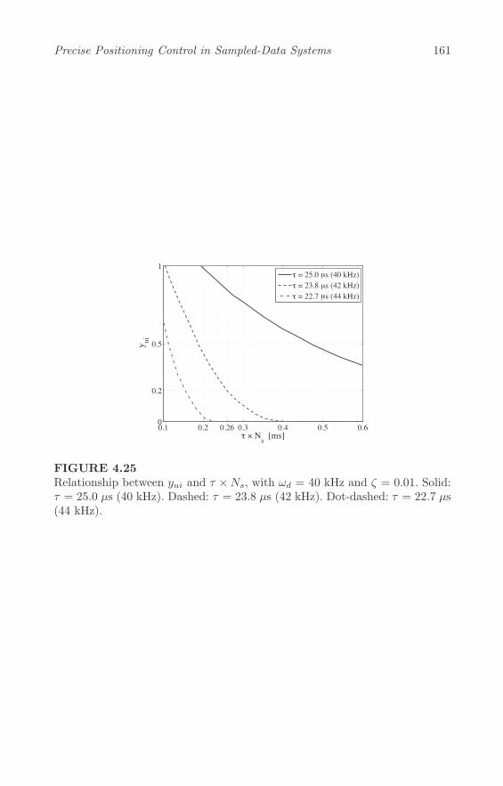
Precise Positioning Control in Sampled-Data Systems 161
0.1 0.2 0.26 0.3 0.4 0.5 0.60
0.2
0.5
1
τ × Ns [ms]
yui
τ = 25.0 s (40 kHz)τ = 23.8 s (42 kHz)τ = 22.7 s (44 kHz)
μμμ
FIGURE 4.25Relationship between yui and τ ×Ns, with ωd = 40 kHz and ζ = 0.01. Solid:τ = 25.0 μs (40 kHz). Dashed: τ = 23.8 μs (42 kHz). Dot-dashed: τ = 22.7 μs(44 kHz).
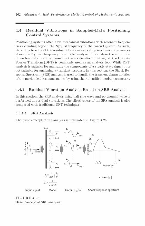
162 Advances in High-Performance Motion Control of Mechatronic Systems
4.4 Residual Vibrations in Sampled-Data PositioningControl Systems
Positioning systems often have mechanical vibrations with resonant frequen-cies extending beyond the Nyquist frequency of the control system. As such,the characteristics of the residual vibrations caused by mechanical resonancesabove the Nyquist frequency have to be analyzed. To analyze the amplitudeof mechanical vibrations caused by the acceleration input signal, the DiscreteFourier Transform (DFT) is commonly used as an analysis tool. While DFTanalysis is suitable for analyzing the components of a steady-state signal, it isnot suitable for analyzing a transient response. In this section, the Shock Re-sponse Spectrum (SRS) analysis is used to handle the transient characteristicsof the mechanical resonant modes by using their identified modal parameters.
4.4.1 Residual Vibration Analysis Based on SRS Analysis
In this section, the SRS analysis using half-sine wave and polynomial wave isperformed on residual vibrations. The effectiveness of the SRS analysis is alsocompared with traditional DFT techniques.
4.4.1.1 SRS Analysis
The basic concept of the analysis is illustrated in Figure 4.26.
FIGURE 4.26Basic concept of SRS analysis.
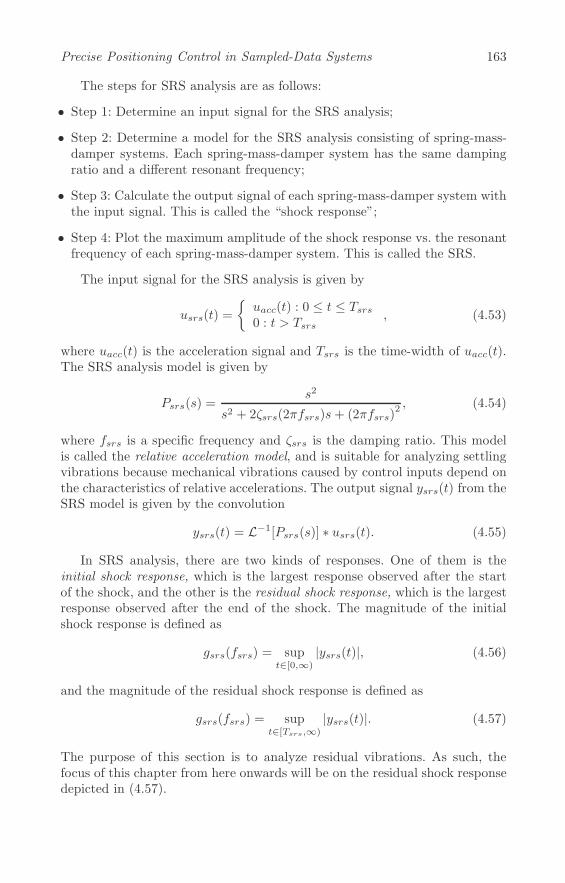
Precise Positioning Control in Sampled-Data Systems 163
The steps for SRS analysis are as follows:
• Step 1: Determine an input signal for the SRS analysis;
• Step 2: Determine a model for the SRS analysis consisting of spring-mass-damper systems. Each spring-mass-damper system has the same dampingratio and a different resonant frequency;
• Step 3: Calculate the output signal of each spring-mass-damper system withthe input signal. This is called the “shock response”;
• Step 4: Plot the maximum amplitude of the shock response vs. the resonantfrequency of each spring-mass-damper system. This is called the SRS.
The input signal for the SRS analysis is given by
usrs(t) =
{uacc(t) : 0 ≤ t ≤ Tsrs0 : t > Tsrs
, (4.53)
where uacc(t) is the acceleration signal and Tsrs is the time-width of uacc(t).The SRS analysis model is given by
Psrs(s) =s2
s2 + 2ζsrs(2πfsrs)s+ (2πfsrs)2 , (4.54)
where fsrs is a specific frequency and ζsrs is the damping ratio. This modelis called the relative acceleration model, and is suitable for analyzing settlingvibrations because mechanical vibrations caused by control inputs depend onthe characteristics of relative accelerations. The output signal ysrs(t) from theSRS model is given by the convolution
ysrs(t) = L−1[Psrs(s)] ∗ usrs(t). (4.55)
In SRS analysis, there are two kinds of responses. One of them is theinitial shock response, which is the largest response observed after the startof the shock, and the other is the residual shock response, which is the largestresponse observed after the end of the shock. The magnitude of the initialshock response is defined as
gsrs(fsrs) = supt∈[0,∞)
|ysrs(t)|, (4.56)
and the magnitude of the residual shock response is defined as
gsrs(fsrs) = supt∈[Tsrs,∞)
|ysrs(t)|. (4.57)
The purpose of this section is to analyze residual vibrations. As such, thefocus of this chapter from here onwards will be on the residual shock responsedepicted in (4.57).

164 Advances in High-Performance Motion Control of Mechatronic Systems
4.4.1.2 SRS Analysis Using Half-Sine Wave
To show the characteristics of residual vibrations in sampled-data controlsystems, SRS analyses are performed using half-sine waves that are widelyemployed as acceleration signals in SRS analyses. The acceleration signal usingthe half-sine wave is given by
uc(t) = sinπt
Tsrs, 0 ≤ t ≤ Tsrs. (4.58)
The acceleration signal using the half-sine wave with a Zero-Order-Hold(ZOH) whose sampling time Tzoh is given by
uzoh(t) = uc(nTzoh), nTzoh ≤ t < (n+ 1)Tsrs, (4.59)
where n is the sample number. The half-sine waves are shown in Figure 4.27.The maximum amount of acceleration is 1 m/s2, and the width of the Tsrs =0.5 ms.
0 0.1 0.2 0.3 0.4 0.5 0.6
0
0.2
0.4
0.6
0.8
1
Time [ms]
Acc
eler
atio
n [m
/s2 ]
w/ ZOHw/o ZOH
FIGURE 4.27Time responses of half-sine waves for SRS analysis. Dashed: with ZOH at asampling time of 25 μs (sampling frequency of 40 kHz). Solid: without ZOH.
A comparison of the results of the SRS analysis with and without the ZOHis shown in Figure 4.28. In this figure, ζsrs = 0. The SRS result without theZOH shows that residual vibration is large only when the resonant frequency isaround 1.4 kHz. In contrast, the SRS result with the ZOH shows that residualvibration is large when the resonant frequencies are around 1.4 kHz, 38.6 kHz,41.4 kHz, 78.6 kHz, and 81.4 kHz. This means that the large magnitude ofthe SRS at low frequencies is spread over all of the aliasing frequencies dueto the effects of the sampler in the ZOH. Consequently, the magnitude of theSRS around the Nyquist frequency and its integer multiples is small, and themagnitude of the SRS around the sampling frequency and its integer multiplesis large.

Precise Positioning Control in Sampled-Data Systems 165
0 20 40 60 80 100−50
−40
−30
−20
−10
0
10
Frequency [kHz]
Mag
nitu
de [d
B]
w/ ZOHw/o ZOH
FIGURE 4.28Comparison of SRS results with and without the ZOH (ζsrs = 0). Dashed:with ZOH. Solid: without ZOH.
To evaluate the effects of the damping ratio, two values of ζsrs given byζsrs = 0 and ζsrs = 0.005 are used for SRS analysis using the half-sine waveshown by the dashed line in Figure 4.28. In Figure 4.28, the case of ζsrs =0 means that the mechanical resonance has no damping, and ζsrs = 0.005means that the mechanical resonance has an average damping ratio.
In Figure 4.29, the SRS result with ζsrs = 0 shows points with nearly zero-magnitude at regular frequency intervals. These points are dependent on theperiod of the half-sine wave and the ZOH. The SRS result with ζsrs = 0.005shows that increasing the damping ratio of the resonant mode will result in adecrease in the residual vibration at almost all frequencies, except those nearthe zero-magnitude frequencies of the case where ζsrs = 0.
Figure 4.30 shows the results of the shock response ysrs(t) using ζsrs =0.005, with the half-sine wave shown by the dashed line in Figure 4.27. Inthis figure, (a) shows the result with fsrs = 20 kHz which coincides with theNyquist frequency of the ZOH, (b) shows the result with fsrs = 40 kHz whichcoincides with the sampling frequency of the ZOH, and (c) shows the resultwith fsrs = 38.6 kHz. Figure 4.27 also shows that the maximum value of theysrs(t) occurs when fsrs = 38.6 kHz. In particular, the residual vibration ofysrs(t) with fsrs = 38.6 kHz is far larger than the residual vibrations withfsrs = 20 kHz, or fsrs = 40 kHz.
To show the effects of the period of the half-sine wave, two half-sine wavesare used for SRS analysis. In Figure 4.31, the dashed line represents the half-sine wave whose period is 0.5 ms, and the solid line represents the half-sinewave whose period is 1 ms. The results of SRS analysis of these half-sine waveswith ζsrs = 0 are shown in Figure 4.32. The SRS result with the half-sinewave whose period is 1 ms shows that the residual vibration is largest when

166 Advances in High-Performance Motion Control of Mechatronic Systems
0 20 40 60 80 100−30
−25
−20
−15
−10
−5
0
5
10
15
Frequency [kHz]
Mag
nitu
de [d
B]
ζ=0ζ=0.005
(a) SRS below 100 kHz
36 37 38 39 40 41 42 43 44−25
−20
−15
−10
−5
0
5
10
Frequency [kHz]
Mag
nitu
de [d
B]
ζ=0ζ=0.005
(b) Close-up of SRS around the sampling frequency
FIGURE 4.29SRS of half-sine wave whose period is 0.5 ms, with ZOH. Solid: ζsrs = 0.005.Dashed: ζsrs = 0.
the resonant frequencies are around 700 Hz, 39.3 kHz, and 40.7 kHz. This isbecause the distance between the frequency around the sampling frequencywhere the magnitude of the SRS is largest and the sampling frequency dependson the period of the half-sine wave.
4.4.1.3 SRS Analysis Using Polynomial Wave
The half-sine wave is widely employed as an acceleration signal in SRS anal-yses. However, feedforward control systems employing time polynomials arewidely used in positioning control systems with a controlled object that canbe modeled as a rigid-body mode using a double integrator. As such, SRS

Precise Positioning Control in Sampled-Data Systems 167
0 0.1 0.2 0.3 0.4 0.5 0.6 0.7 0.8−2
−1
0
1
2
Am
plitu
de
Time [ms]
(a) fsrs: 20 kHz (the Nyquist frequency)
0 0.1 0.2 0.3 0.4 0.5 0.6 0.7 0.8−2
−1
0
1
2
Am
plitu
de
Time [ms]
(b) fsrs: 40 kHz (the sampling frequency)
0 0.1 0.2 0.3 0.4 0.5 0.6 0.7 0.8−2
−1
0
1
2
Am
plitu
de
Time [ms]
(c) fsrs: 38.6 kHz
FIGURE 4.30Results of shock response ysrs(t) using ζsrs = 0.005, with the half-sine wavesshown by the dashed line in Figure 4.27.
analyses using acceleration inputs based on polynomials-in-time are describedin this section.
A discrete-time acceleration input signal Fpoly(n) which satisfies theboundary conditions including the characteristics of a ZOH is generated withthe sampled-data polynomial given by [4]
Fpoly(n) =840n2(n−N)3(−10 + (7n− 3N)N(1 +N2))Pt
N(N2 − 4)(N2 − 1)(N2 + 5)(10 + 3(N2 +N4))τ2ff, (4.60)
where N is the period of the acceleration input in terms of samples and Pt isthe target of the moving span in meters. In this case, the acceleration signalfor SRS analysis is given by
uacc(t) = Fpoly(n), nTzoh ≤ t < (n− 1)Tzoh. (4.61)
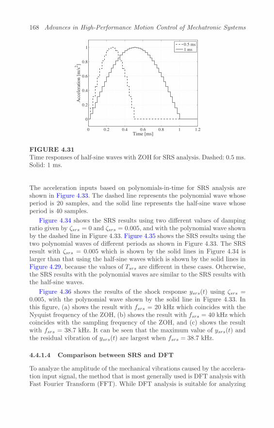
168 Advances in High-Performance Motion Control of Mechatronic Systems
0 0.2 0.4 0.6 0.8 1 1.2
0
0.2
0.4
0.6
0.8
1
Time [ms]
Acc
eler
atio
n [m
/s2 ]
0.5 ms1 ms
FIGURE 4.31Time responses of half-sine waves with ZOH for SRS analysis. Dashed: 0.5 ms.Solid: 1 ms.
The acceleration inputs based on polynomials-in-time for SRS analysis areshown in Figure 4.33. The dashed line represents the polynomial wave whoseperiod is 20 samples, and the solid line represents the half-sine wave whoseperiod is 40 samples.
Figure 4.34 shows the SRS results using two different values of dampingratio given by ζsrs = 0 and ζsrs = 0.005, and with the polynomial wave shownby the dashed line in Figure 4.33. Figure 4.35 shows the SRS results using thetwo polynomial waves of different periods as shown in Figure 4.33. The SRSresult with ζsrs = 0.005 which is shown by the solid lines in Figure 4.34 islarger than that using the half-sine waves which is shown by the solid lines inFigure 4.29, because the values of Tsrs are different in these cases. Otherwise,the SRS results with the polynomial waves are similar to the SRS results withthe half-sine waves.
Figure 4.36 shows the results of the shock response ysrs(t) using ζsrs =0.005, with the polynomial wave shown by the solid line in Figure 4.33. Inthis figure, (a) shows the result with fsrs = 20 kHz which coincides with theNyquist frequency of the ZOH, (b) shows the result with fsrs = 40 kHz whichcoincides with the sampling frequency of the ZOH, and (c) shows the resultwith fsrs = 38.7 kHz. It can be seen that the maximum value of ysrs(t) andthe residual vibration of ysrs(t) are largest when fsrs = 38.7 kHz.
4.4.1.4 Comparison between SRS and DFT
To analyze the amplitude of the mechanical vibrations caused by the accelera-tion input signal, the method that is most generally used is DFT analysis withFast Fourier Transform (FFT). While DFT analysis is suitable for analyzing

Precise Positioning Control in Sampled-Data Systems 169
0 10 20 30 40 50 60−30
−25
−20
−15
−10
−5
0
5
10
15
Frequency [kHz]
Mag
nitu
de [d
B]
0.5 ms1 ms
(a) SRS below 60 kHz
36 37 38 39 40 41 42 43 44−25
−20
−15
−10
−5
0
5
10
Frequency [kHz]
Mag
nitu
de [d
B]
0.5 ms1 ms
(b) Close-up of SRS around the sampling frequency
FIGURE 4.32Comparison of SRS results between the half-sine wave having a width of 0.5ms and the half-sine wave having a width of 1 ms. Dashed: 0.5 ms. Solid: 1 ms.
the contents of steady-state characteristics, it is not suitable for analyzingtransient characteristics.
To show the difference between DFT and SRS analyses, a DFT analysis ofthe acceleration input is performed. Figure 4.37 shows a comparison betweenthe results of the SRS and that of the DFT analysis with the polynomial waveshown by the solid line in Figure 4.33. In this figure, the solid line representsthe DFT result shown using an amplitude spectrum, the dashed line representsthe SRS result with ζsrs = 0, and the dot-dashed line represents the SRSresult with ζsrs = 0.005. These results are normalized so that the maximummagnitude is of 0 dB.
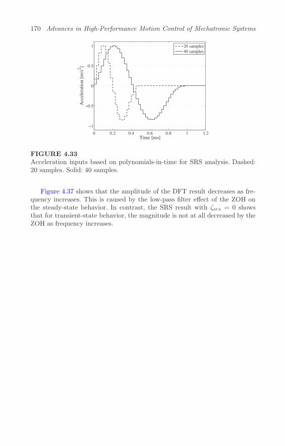
170 Advances in High-Performance Motion Control of Mechatronic Systems
0 0.2 0.4 0.6 0.8 1 1.2−1
−0.5
0
0.5
1
Time [ms]
Acc
eler
atio
n [m
/s2 ]
20 samples40 samples
FIGURE 4.33Acceleration inputs based on polynomials-in-time for SRS analysis. Dashed:20 samples. Solid: 40 samples.
Figure 4.37 shows that the amplitude of the DFT result decreases as fre-quency increases. This is caused by the low-pass filter effect of the ZOH onthe steady-state behavior. In contrast, the SRS result with ζsrs = 0 showsthat for transient-state behavior, the magnitude is not at all decreased by theZOH as frequency increases.
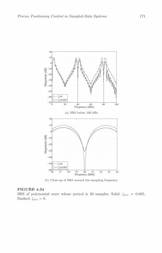
Precise Positioning Control in Sampled-Data Systems 171
0 20 40 60 80 100−70
−60
−50
−40
−30
−20
−10
0
10
20
Frequency [kHz]
Mag
nitu
de [d
B]
ζ=0ζ=0.005
(a) SRS below 100 kHz
36 37 38 39 40 41 42 43 44−60
−50
−40
−30
−20
−10
0
10
20
Frequency [kHz]
Mag
nitu
de [d
B]
ζ=0ζ=0.005
(b) Close-up of SRS around the sampling frequency
FIGURE 4.34SRS of polynomial wave whose period is 20 samples. Solid: ζsrs = 0.005.Dashed: ζsrs = 0.

172 Advances in High-Performance Motion Control of Mechatronic Systems
0 10 20 30 40 50 60−70
−60
−50
−40
−30
−20
−10
0
10
20
Frequency [kHz]
Mag
nitu
de [d
B]
20 samples40 samples
(a) SRS below 60 kHz
36 37 38 39 40 41 42 43 44−60
−50
−40
−30
−20
−10
0
10
20
Frequency [kHz]
Mag
nitu
de [d
B]
20 samples40 samples
(b) Close-up of SRS around the sampling frequency
FIGURE 4.35Comparison of SRS results between the polynomial wave with a period of 20samples and the polynomial wave with a period of 40 samples using ζsrs = 0.Dashed: 20 samples. Solid: 40 samples.

Precise Positioning Control in Sampled-Data Systems 173
0 0.5 1 1.5−2
−1
0
1
2
Am
plitu
de
Time [ms]
(a) fsrs: 20 kHz (the Nyquist frequency)
0 0.5 1 1.5−2
−1
0
1
2
Am
plitu
de
Time [ms]
(b) fsrs: 40 kHz (the sampling frequency)
0 0.5 1 1.5−2
−1
0
1
2
Am
plitu
de
Time [ms]
(c) fsrs: 38.7 kHz
FIGURE 4.36Results of shock response ysrs(t) using ζsrs = 0.005 with the polynomial waveshown by the solid line in Figure 4.33.
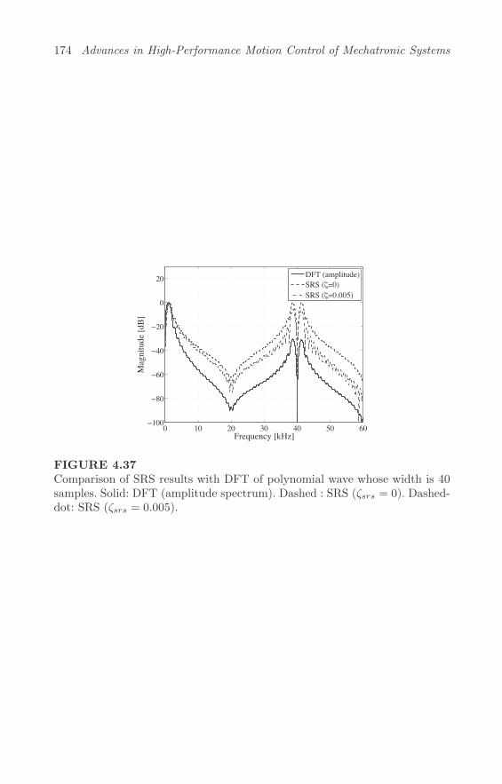
174 Advances in High-Performance Motion Control of Mechatronic Systems
0 10 20 30 40 50 60−100
−80
−60
−40
−20
0
20
Frequency [kHz]
Mag
nitu
de [d
B]
DFT (amplitude)SRS (ζ=0)SRS (ζ=0.005)
FIGURE 4.37Comparison of SRS results with DFT of polynomial wave whose width is 40samples. Solid: DFT (amplitude spectrum). Dashed : SRS (ζsrs = 0). Dashed-dot: SRS (ζsrs = 0.005).
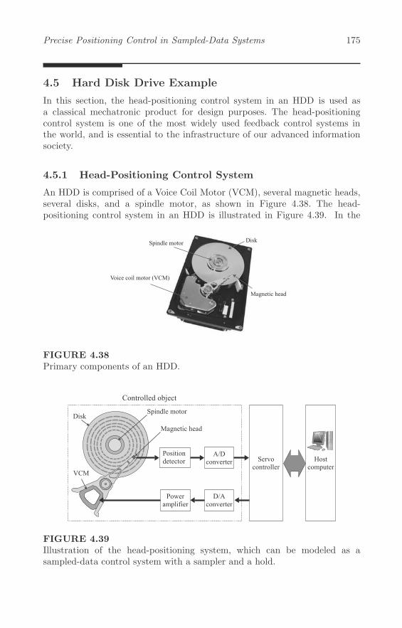
Precise Positioning Control in Sampled-Data Systems 175
4.5 Hard Disk Drive Example
In this section, the head-positioning control system in an HDD is used asa classical mechatronic product for design purposes. The head-positioningcontrol system is one of the most widely used feedback control systems inthe world, and is essential to the infrastructure of our advanced informationsociety.
4.5.1 Head-Positioning Control System
An HDD is comprised of a Voice Coil Motor (VCM), several magnetic heads,several disks, and a spindle motor, as shown in Figure 4.38. The head-positioning control system in an HDD is illustrated in Figure 4.39. In the
FIGURE 4.38Primary components of an HDD.
FIGURE 4.39Illustration of the head-positioning system, which can be modeled as asampled-data control system with a sampler and a hold.

176 Advances in High-Performance Motion Control of Mechatronic Systems
head-positioning control system, the various sources of disturbances includeperiodic disturbances caused by disk rotation known as repeatable runout, ef-fects of torque noise, and mechanical vibrations excited by the airflow inducedby the spinning disks, etc. The controlled variable is the head-position signal,which is generated from embedded information on the disks and read at afixed time interval. This means that the head-position signal is only availableas a discrete-time signal. The control input is an input command value toa VCM driver amplifier, which is calculated by a digital signal processor atcertain intervals. As such, the head-positioning control system can be thoughtof as a sampled-data control system that has a sampler and a hold.
4.5.1.1 Controlled Object
In this section, it is assumed that gain of the controlled object Pc(jω) in thecontinuous-time system is negligible when ω > 2ωs. In order to reduce thecalculation load, the frequency response of Pc(jω) is defined as
Pc(jω0) =
{Pc0(jω0), |ω0| ≤ 2ωs,0, |ω0| > 2ωs.
(4.62)
Pc0 is assumed to be given by the product of the mechanical model Ps andthe equivalent delay-time model Pdl as
Pc0(s) = Ps(s)Pdl(s). (4.63)
The mechanical model Ps is given by
Ps(s) = Kp
ψ∑l=1
αk(l)
s2 + 2ζk(l)ωnk(l)s+ ωnk(l)2 , (4.64)
where ψ is the number of modes, αk is the residue of each mode, ωnk andζk are the natural frequency in rad/s and damping ratio of the resonance,respectively, andKp is the plant gain. These parameters are chosen so that thefrequency response of the model coincides with the measured result indicatedby the solid line in Figure 4.40. To be more precise, ψ = 7 as the order of themodel is 14, Kp = 4.3× 10⁷, and the values of the other parameters are listedin Table 4.1. The dashed line in Figure 4.40 represents the frequency responseof this mathematical model.
The equivalent time delay model Pdl includes the characteristics of thedelay-time element, and is given by
Pdl(s) = e−τs, (4.65)
where τ is the equivalent time delay of 10 μs in this study.

Precise Positioning Control in Sampled-Data Systems 177
103 104−40
−20
0
20
Frequency [Hz]
Gai
n [d
B]
Measurement dataMathematical model
103 104−360
−270
−180
−90
0
Frequency [Hz]
Phas
e [d
eg.]
Measurement dataMathematical model
FIGURE 4.40Frequency response of the mechanical system.
TABLE 4.1Parameters of Ps(s)
l ωnk(l) αk(l) ζk(l)1 0 1.00 02 2π4100 −1.30 0.013 2π5700 −0.03 0.014 2π6200 −0.08 0.015 2π7650 0.12 0.026 2π8900 −0.13 0.027 2π9800 −0.35 0.03
4.5.2 Sensitivity and Complementary Sensitivity TransferFunctions
In this example, the head-positioning control system uses a multi-rate filter,and its block diagram is shown in Figure 4.2. The sampling time Ts is set as153.5 μs, resulting in ωs = 2π6516 rad/s, and the multi-rate number m is setas 4. The multi-rate hold Hm is the ZOH, and its transfer characteristic isgiven by
Hm(s) =1− e−
sTs4
s. (4.66)
The interpolator Ip consists of an up-sampler and an interpolation filter. Thetransfer function of the interpolation filter can be given by
Ip(z) = 1 + z−1 + z−2 + z−3. (4.67)
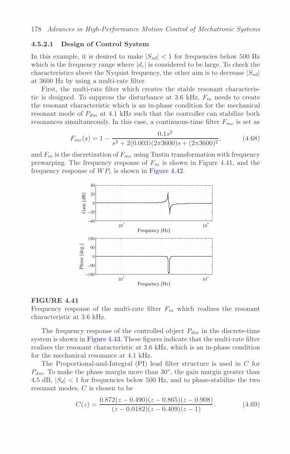
178 Advances in High-Performance Motion Control of Mechatronic Systems
4.5.2.1 Design of Control System
In this example, it is desired to make |Ssd| < 1 for frequencies below 500 Hzwhich is the frequency range where |dc| is considered to be large. To check thecharacteristics above the Nyquist frequency, the other aim is to decrease |Ssd|at 3600 Hz by using a multi-rate filter.
First, the multi-rate filter which creates the stable resonant characteris-tic is designed. To suppress the disturbance at 3.6 kHz, Fm needs to createthe resonant characteristic which is an in-phase condition for the mechanicalresonant mode of Pdm at 4.1 kHz such that the controller can stabilize bothresonances simultaneously. In this case, a continuous-time filter Fmc is set as
Fmc(s) = 1− 0.1s2
s2 + 2(0.003)(2π3600)s+ (2π3600)2, (4.68)
and Fm is the discretization of Fmc using Tustin transformation with frequencyprewarping. The frequency response of Fm is shown in Figure 4.41, and thefrequency response of WPc is shown in Figure 4.42.
103 104−40
−20
0
20
40
Gai
n [d
B]
Frequency [Hz]
103 104−180
−90
0
90
180
Phas
e [d
eg.]
Frequency [Hz]
FIGURE 4.41Frequency response of the multi-rate filter Fm which realizes the resonantcharacteristic at 3.6 kHz.
The frequency response of the controlled object Pdm in the discrete-timesystem is shown in Figure 4.43. These figures indicate that the multi-rate filterrealizes the resonant characteristic at 3.6 kHz, which is an in-phase conditionfor the mechanical resonance at 4.1 kHz.
The Proportional-and-Integral (PI) lead filter structure is used in C forPdm. To make the phase margin more than 30◦, the gain margin greater than4.5 dB, |Sd| < 1 for frequencies below 500 Hz, and to phase-stabilize the tworesonant modes, C is chosen to be
C(z) =0.872(z − 0.490)(z − 0.865)(z − 0.908)
(z − 0.0182)(z − 0.409)(z − 1). (4.69)

Precise Positioning Control in Sampled-Data Systems 179
103 104
−60
−40
−20
0
20
Gai
n [d
B]
Frequency [Hz]
103 104−360
−270
−180
−90
0
Phas
e [d
eg.]
Frequency [Hz]
FIGURE 4.42Frequency response of WPc.
0 500 1000 1500 2000 2500 3000−40
−20
0
20
Gai
n [d
B]
Frequency [Hz]
0 500 1000 1500 2000 2500 3000−360
−270
−180
−90
0
Phas
e [d
eg.]
Frequency [Hz]
FIGURE 4.43Frequency response of controlled object Pdm in discrete-time system.
The frequency response of C is shown in Figure 4.44, and the frequency re-sponse of the open-loop characteristics PdmC of the discrete-time system isshown in Figure 4.45.
The magnitude response of∑∞
l=−∞, �=0 |Γm(ω0, l)| is shown in Figure 4.46.
This figure indicates that the control system makes∑∞
l=−∞, �=0 |Γm(ω0, l)|small at frequencies below 500 Hz and at 3.6 kHz.
The frequency responses of |Sd| and |Td| are shown in Figure 4.47. The fre-quency responses of |Ssd| and |Tsd| are shown in Figure 4.48, and the frequencyresponses of |SΔ| and |TΔ| are shown in Figure 4.49.
It is clear that the characteristics of the sensitivity and complementary sen-
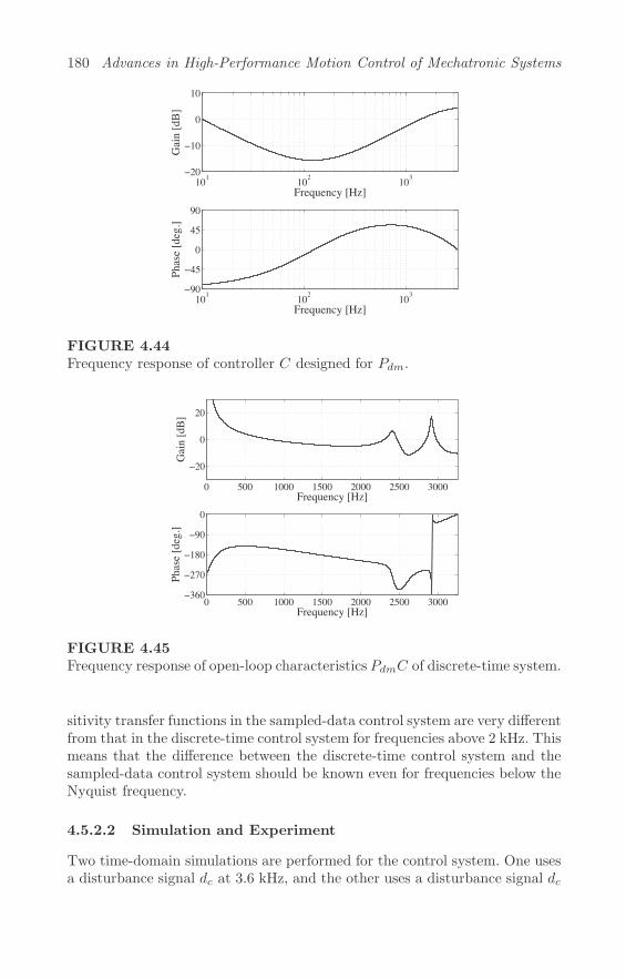
180 Advances in High-Performance Motion Control of Mechatronic Systems
101 102 103−20
−10
0
10
Gai
n [d
B]
Frequency [Hz]
101 102 103−90
−45
0
45
90
Phas
e [d
eg.]
Frequency [Hz]
FIGURE 4.44Frequency response of controller C designed for Pdm.
0 500 1000 1500 2000 2500 3000
−20
0
20
Gai
n [d
B]
Frequency [Hz]
0 500 1000 1500 2000 2500 3000−360
−270
−180
−90
0
Phas
e [d
eg.]
Frequency [Hz]
FIGURE 4.45Frequency response of open-loop characteristics PdmC of discrete-time system.
sitivity transfer functions in the sampled-data control system are very differentfrom that in the discrete-time control system for frequencies above 2 kHz. Thismeans that the difference between the discrete-time control system and thesampled-data control system should be known even for frequencies below theNyquist frequency.
4.5.2.2 Simulation and Experiment
Two time-domain simulations are performed for the control system. One usesa disturbance signal dc at 3.6 kHz, and the other uses a disturbance signal dc

Precise Positioning Control in Sampled-Data Systems 181
0 0.5 2 2.92 3.64 6 8 10−30
−25
−20
−15
−10
−5
0
5
10
Gai
n [d
B]
Frequency [kHz]
FIGURE 4.46Frequency response of
∑∞l=−∞, �=0 |Γm(ω0, l)|.
0 0.5 2 2.92 3.64 6 8 10−20
−15
−10
−5
0
5
10
Gai
n [d
B]
Frequency [kHz]
|Sd||Td|
FIGURE 4.47Magnitude responses of sensitivity and complementary sensitivity transferfunctions of the discrete-time system. Solid:|Sd|. Dashed: |Td|.
at 2.916 kHz which is an aliasing frequency of 3.6 kHz. In both simulations,the amplitude of dc = 0.1 track pitch and reference r is set to 0.
The simulation results with dc = 3.6 kHz are shown in Figure 4.50, andthe simulation results with dc = 2.916 kHz are shown in Figure 4.51. In bothfigures, yd is indicated by the solid line in (a), yd0 is indicated by the dashedline in (a), yc is indicated by the solid line in (b), and yc0 is indicated by thedashed line in (b).

182 Advances in High-Performance Motion Control of Mechatronic Systems
0 0.5 2 2.92 3.64 6 8 10−20
−15
−10
−5
0
5
10
Gai
n [d
B]
Frequency [kHz]
|Ssd||Tsd|
FIGURE 4.48Magnitude responses of sensitivity and complementary sensitivity transferfunctions of the sampled-data control system. Solid: |Ssd|. Dashed: |Tsd|.
0 0.5 2 2.92 3.64 6 8 100
5
10
15
20
25
30
Gai
n [d
B]
Frequency [kHz]
|S ||T |
ΔΔ
FIGURE 4.49Magnitude responses of |SΔ| and |TΔ| which illustrate the difference between|Ssd| and |Sd|, and the difference between |Tsd| and |Td|, respectively. Solid:|SΔ|. Dashed: |TΔ|.
The simulation results with dc = 3.6 kHz show that
||yc(t)||∞||dc(t)||∞ = 0.18,
||yc0(t)||∞||dc(t)||∞ = 0.92,
||yd(t)||∞||dc(t)||∞ = 0.13,
||yd0(t)||∞||dc(t)||∞ = 0.90, (4.70)

Precise Positioning Control in Sampled-Data Systems 183
0 0.5 1 1.5 2 2.5 3−0.2
−0.15
−0.1
−0.05
0
0.05
0.1
0.15
0.2
Time [ms]
Posi
tion
[trac
k pi
tch]
ydyd0
(a) yd and yd0
0 0.5 1 1.5 2 2.5 3−0.2
−0.15
−0.1
−0.05
0
0.05
0.1
0.15
0.2
Time [ms]
Posi
tion
[trac
k pi
tch]
ycyc0
(b) yc and yc0
FIGURE 4.50Simulated head-position with disturbance at 3.6 kHz.
and the simulation results with dc = 2.916 kHz show that
||yc(t)||∞||dc(t)||∞ = 1.85,
||yc0(t)||∞||dc(t)||∞ = 0.92,
||yd(t)||∞||dc(t)||∞ = 0.13,
||yd0(t)||∞||dc(t)||∞ = 0.90. (4.71)
These results indicate that the simulation results are almost identical to theresults in Figures 4.47 and 4.48.
To validate the effects of the proposed method, experiments are conductedusing conditions which are similar to those of the simulations. In these exper-iments, yc0 and yc are discrete-time signals with a sampling time of 38.4 μs

184 Advances in High-Performance Motion Control of Mechatronic Systems
0 0.5 1 1.5 2 2.5 3−0.2
−0.15
−0.1
−0.05
0
0.05
0.1
0.15
0.2
Time [ms]
Posi
tion
[trac
k pi
tch]
ydyd0
(a) yd and yd0
0 0.5 1 1.5 2 2.5 3−0.2
−0.15
−0.1
−0.05
0
0.05
0.1
0.15
0.2
Time [ms]
Posi
tion
[trac
k pi
tch]
ycyc0
(b) yc and yc0
FIGURE 4.51Simulated head-position with disturbance at 2.916 kHz.
which is Ts
4 . This is because the continuous-time signal cannot be measured inactual head-positioning systems. The experimental results with dc = 3.6 kHzare shown in Figure 4.52, and the results with dc = 2.916 kHz are shown inFigure 4.53. In both figures, yd is indicated by the solid line in (a), yd0 isindicated by the dashed line in (a), yc is indicated by the solid line in (b), yc0is indicated by the dashed line in (b). These experimental results show thatthey are also almost the same as the simulation results.

Precise Positioning Control in Sampled-Data Systems 185
0 0.5 1 1.5 2 2.5 3−0.2
−0.15
−0.1
−0.05
0
0.05
0.1
0.15
0.2
Time [ms]
Posi
tion
[trac
k pi
tch]
ydyd0
(a) yd and yd0
0 0.5 1 1.5 2 2.5 3−0.2
−0.15
−0.1
−0.05
0
0.05
0.1
0.15
0.2
Time [ms]
Posi
tion
[trac
k pi
tch]
ycyc0
(b) yc and yc0
FIGURE 4.52Experimental results illustrating head-position with disturbance at 3.6 kHz.
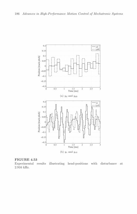
186 Advances in High-Performance Motion Control of Mechatronic Systems
0 0.5 1 1.5 2 2.5 3−0.2
−0.15
−0.1
−0.05
0
0.05
0.1
0.15
0.2
Time [ms]
Posi
tion
[trac
k pi
tch]
ydyd0
(a) yd and yd0
0 0.5 1 1.5 2 2.5 3−0.2
−0.15
−0.1
−0.05
0
0.05
0.1
0.15
0.2
Time [ms]
Posi
tion
[trac
k pi
tch]
ycyc0
(b) yc and yc0
FIGURE 4.53Experimental results illustrating head-positions with disturbance at2.916 kHz.

Precise Positioning Control in Sampled-Data Systems 187
4.5.3 Unobservable Oscillations
In this example, the unobservable magnitudes for oscillations in the head-positioning control system are analyzed. The controlled object has a primarymechanical resonance at 4.1 kHz and other mechanical resonances are muchsmaller than the primary resonance as shown by Figure 4.40 and Table. 4.1. Assuch, the focus in this example is on the unobservable oscillation of the primaryresonant mode. The damped natural frequency ωd = 2π4100 rad/s and thedamping ratio ζ = 0.01 as indicated by Table. 4.1, and yui are calculated.
The dependence of yui on the sampling frequency is shown in Figure 4.54.In the head-positioning control system, the number of servo sectors on thedisks must be decided so that the sampling frequency does not coincide withthe unacceptable sampling frequencies shown in Figure 4.54. For example,the solid line shows that most of the frequencies from 1 kHz to 10 kHz areunacceptable sampling frequencies when Ns = 5, and the acceptable levelof unobservable magnitude is 0.1. The dashed line shows that the samplingfrequency cannot be chosen to be around 1.02 kHz, 1.37 kHz, 2.05 kHz, 2.73kHz, 4.10 kHz, 82.0 kHz, and 123 kHz when Ns = 10, and the acceptablelevel of unobservable magnitude is 0.1. The dot-dashed line shows that thesampling frequency cannot be chosen to be around 2.05 kHz, 4.10 kHz, and8.20 kHz when Ns is 20, and the acceptable level of unobservable magnitudeis 0.1.
103 10400.1
0.5
1
Sampling frequency [Hz]
yui
5 sample10 sample20 sample
FIGURE 4.54Relationship between yui and sampling frequency considering the primarymechanical resonance, with ωd = 2π · 4100 and ζ = 0.01. Solid: Ns = 5.Dashed: Ns = 10. Dashed-dot: Ns = 20.
The dependence of yui on the measurement time τ ×Ns for the judgmentof maximum displacement is shown in Figure 4.55. In this figure, the solid linerepresents the result with τ = 244 μs (4.1 kHz), the dashed line represents the

188 Advances in High-Performance Motion Control of Mechatronic Systems
result with τ = 233 μs (4.3 kHz), and the dot-dashed line represents the resultwith τ = 222 μs (4.5 kHz). In the head-positioning control system, the samplenumber for the judgment of the maximum displacement Ns must be decidedso that yui is smaller than the acceptable level of unobservable magnitudecaused by the mechanical resonance at 4.1 kHz. For example, the dashed lineshows that τ × Ns should be more than 3 ms when the acceptable level ofyui = 0.1 and τ = 233 μs (4.3 kHz).
1 2 3 4 50
0.1
0.5
1
1.5
τ × Ns [ms]
yui
τ = 244 s (4.1 kHz)τ = 233 s (4.3 kHz)τ = 222 s (4.5 kHz)
μ
μμμ
FIGURE 4.55Relationship between yui and τ × Ns considering the primary mechanicalresonance. Solid: τ = 244 μs (4.1 kHz). Dashed: τ = 233 μs (4.3 kHz). Dot-dashed: τ = 222 μs (4.5 kHz).
4.5.4 Residual Vibrations
In this example, the residual vibrations of the head-positioning control systemthat uses a Two-Degrees-of-Freedom (TDOF) control system are analyzed.The block diagram of a sampled-data control system based on TDOF controlis shown in Figure 4.56.
C H PcydFp
Fa
++−
+ ycuc S
Hf
e
FIGURE 4.56Block diagram of TDOF control system.
In this example, the results of residual vibrations in track-seeking con-

Precise Positioning Control in Sampled-Data Systems 189
trol are presented. The head-positioning system uses a TDOF control systemshown in Figure 4.57. In this figure, S is a sampler, C is a feedback controller,H is a hold for the feedback control input, Hf is a hold for the accelerationfeedforward control input, and Pc is a controlled object in continuous time.Fa is an acceleration feedforward input signal in discrete time, Fp is a positionfeedforward input signal in discrete time, and Ip is an interpolator that con-sists of a ZOH and an up-sampler.Mf is a discrete-time model that generatesthe position feedforward input Fp from the acceleration feedforward input Fa,uc is the control input in continuous time, yc is a controlled variable in con-tinuous time, yd is a controlled variable in discrete time, and e is a trackingerror signal in discrete time.
C H PcydFp
Fa
++−+ ycucMf SIp
Hf
e
FIGURE 4.57Block diagram of TDOF control system for experiments.
In this system, the sampling times of S and H are denoted as τfb, and thesampling times of Fa and Hf are denoted as τff . To analyze the relationshipbetween the mechanical resonant frequency and the sampling time of the ZOH,three different values of τff are used since the mechanical resonant frequenciesare fixed and only the sampling time of the ZOH can be changed. The samplingtime of the position feedforward input signal Fp, Mf , and Ip is set as τfb sothat the feedback control has the same performance when the sampling timeof the acceleration feedforward input is changed.
4.5.4.1 Feedback Control System
In this control system, the major mechanical modes are Mode 1 which isthe rigid-body mode and Mode 2 which is the primary mechanical resonantmode as listed in Table 4.1. The feedback controller C(z) is given by theproduct of the PI-lead filter Cp(z) and the notch filter Cn(z). Cp(z) providesintegral action, and its phase stabilizes the rigid-body mode. Cn(z) stabilizesthe primary mechanical resonance by decreasing the gain of the resonance.Cp(z) is the discretization of Cpc(s) using bilinear transformation, and Cn(z)is the discretization of Cnc(s) using the pole-zero matching method. Cpc(s)and Cnc(s) provide more than 40◦ phase margin at 1 kHz and a gain marginof more than 5 dB. Cpc(s) and Cnc(s) are given by
Cpc(s) =1318(s+ 628.3)(s+ 1257)
s(s+ 25130)(4.72)
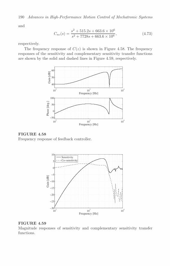
190 Advances in High-Performance Motion Control of Mechatronic Systems
and
Cnc(s) =s2 + 515.2s+ 663.6× 10⁶
s2 + 7728s+ 663.6× 10⁶, (4.73)
respectively.
The frequency response of C(z) is shown in Figure 4.58. The frequencyresponses of the sensitivity and complementary sensitivity transfer functionsare shown by the solid and dashed lines in Figure 4.59, respectively.
102 103 104
40
50
60
Gai
n [d
B]
Frequency [Hz]
102 103 104−50
0
50
100
Phas
e [d
eg.]
Frequency [Hz]
FIGURE 4.58Frequency response of feedback controller.
102 103 104−30
−25
−20
−15
−10
−5
0
5
10
Gai
n [d
B]
Frequency [Hz]
SensitivityCo−sensitivity
FIGURE 4.59Magnitude responses of sensitivity and complementary sensitivity transferfunctions.

Precise Positioning Control in Sampled-Data Systems 191
4.5.4.2 Feedforward Control System
The acceleration input Fa(n) is generated with the sampled-data polynomialshown in (4.60). To evaluate the relationship between the mechanical resonantfrequency and the sampling frequency of the ZOH, three acceleration inputswhose target seek spans Pt of 500 tracks are used. For the first input, τffwhich is the sampling time of the ZOH Hf is 115 μs, and target seek timeN = 40. For the second input, τff = 230 μs and N = 20. For the thirdinput, τff = 307 μs and N = 15. The time responses of Fa(n) for the threecases where τff = 115 μs, τff = 230 μs, and τff = 307 μs are shown inFigure 4.60(a) using solid, dashed, and dashed-dot lines, respectively.
0 0.5 1 1.5 2 2.5 3 3.5 4 4.5−200
−150
−100
−50
0
50
100
150
200
Time [ms]
Con
trol i
nput
[m/s
2 ]
115 s230 s307 sμ
μμ
(a) Acceleration feedforward inputs
0 0.5 1 1.5 2 2.5 3 3.5 4 4.50
100
200
300
400
500
Time [ms]
Hea
d po
sitio
n [tr
ack]
115 s230 s307 s
μμμ
(b) Position feedforward inputs
FIGURE 4.60Time responses of feedforward inputs. Solid: τff = 115 μs. Dashed: τff =230 μs. Dashed-dot: τff = 307 μs.

192 Advances in High-Performance Motion Control of Mechatronic Systems
The position feedforward input Fp(n) is generated by the reference modelMf (z) because the computational burden is lower than that of computing thepolynomial for the position feedforward input. Fa(n) is the input to Mf (z)via Ip(z), and the output signal from Mf (z) becomes Fp(n).
Mf (z) can be calculated from the continuous-time transfer function Pf (s)by including the delay time and performing discretization with ZOH. Pf (s) isgiven by
Pf (s) = Kp
(1
s2+
αfs2 + 2ζfωfs+ ω2
f
), (4.74)
where αf is the residue of the resonant mode, and ωf and ζf are the naturalfrequency and damping ratio of the resonant mode, respectively.
ζf should be much larger than the damping ratio of the primary mechan-ical resonance to prevent oscillation in the reference model. To calculate theposition feedforward input, αf , ζf , and ωf are determined so that the fre-quency response of Pf (s) coincides with the measured frequency response ofthe mechanical system for frequencies below 2 kHz. As such, αf = −1.3,ωf = 2π3950 rad/s, and ζf = 0.3. By including the delay time Tdl and dis-cretizing Pf (s) using a ZOH, Mf (z) is given by
Mf(z) = −3.157× 10⁻⁶ (z − 14.34)(z − 0.3574)(z + 0.1314)(z + 2.408)
z(z − 1)2(z2 − 0.9245z + 0.5648).
(4.75)The position feedforward inputs Fp(n) for the cases where τff = 115 μs,τff = 230 μs, and τff = 307 μs are shown in Figure 4.60(b) using solid,dashed, and dashed-dot lines, respectively.
4.5.4.3 SRS Analysis
The SRS results of the acceleration input in Figure 4.60(a) for the cases ofτff = 115 μs, τff = 230 μs, and τff = 307 μs are shown in Figure 4.61 usingsolid, dashed, and dashed-dot lines, respectively. ζsrs = 0.01 because it shouldbe approximately the same as that of the primary mechanical resonance at4.1 kHz shown in Table 4.1. It should be noted that the damping ratio of thismechanical resonance in the head-positioning system of HDDs is relativelylarge.
The controlled object has a primary mechanical resonance at 4.1 kHz asshown by Figure 4.40 and Table 4.1. The SRS results show that the magnitudeof the SRS at 4.1 kHz is smallest in the first case where τff = 115 μs, becausethe Nyquist frequency of the ZOH is about 4.3 kHz. The magnitude of the SRSat 4.1 kHz is largest in the second case where τff = 230 μs since the samplingfrequency of the ZOH is about 4.3 kHz. In the third case where τff = 307 μs,the magnitude of the SRS at 4.1 kHz is smaller than that of the second caseeven though the sampling time is longer than that of the second case.

Precise Positioning Control in Sampled-Data Systems 193
0 2 4 6 8 10−40
−20
0
20
40
60
Frequency [kHz]
Mag
nitu
de [d
B]
115 s230 s307 s
μ
μμμ
FIGURE 4.61Results of SRS. Solid: τff = 115 μs. Dashed: τff = 230 μs. Dashed-dot:τff = 307 μs.
4.5.4.4 Simulation and Experimental Results
To verify the results of the SRS analysis, simulations and experiments are con-ducted for track-seeking control. The simulation results for the head-positionsare shown in Figure 4.62, and those of the tracking error signals are shownin Figure 4.63. The experimental results for the head-positions are shown inFigure 4.64, and those of the tracking error signals are shown in Figure 4.65.
2.5 3 3.5 4 4.5 5 5.5 6499
499.5
500
500.5
501
Time [ms]
Posi
tion
[trac
k]
115 s230 s307 s
μμμ
FIGURE 4.62Simulation results for head positions. Solid: τff = 115 μs. Dashed: τff =230 μs. Dashed-dot: τff = 307 μs.
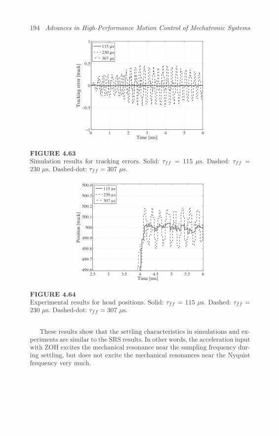
194 Advances in High-Performance Motion Control of Mechatronic Systems
0 1 2 3 4 5 6−1
−0.5
0
0.5
1
Time [ms]
Trac
king
err
or [t
rack
]
115 s230 s307 sμ
μμ
FIGURE 4.63Simulation results for tracking errors. Solid: τff = 115 μs. Dashed: τff =230 μs. Dashed-dot: τff = 307 μs.
2.5 3 3.5 4 4.5 5 5.5 6499.6
499.7
499.8
499.9
500
500.1
500.2
500.3
500.4
Time [ms]
Posi
tion
[trac
k]
115 s230 s307 sμ
μμ
FIGURE 4.64Experimental results for head positions. Solid: τff = 115 μs. Dashed: τff =230 μs. Dashed-dot: τff = 307 μs.
These results show that the settling characteristics in simulations and ex-periments are similar to the SRS results. In other words, the acceleration inputwith ZOH excites the mechanical resonance near the sampling frequency dur-ing settling, but does not excite the mechanical resonances near the Nyquistfrequency very much.
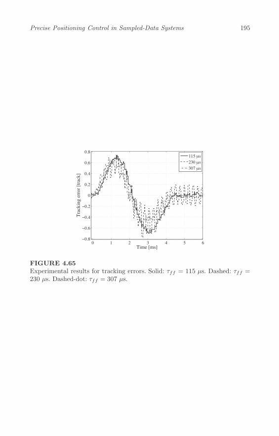
Precise Positioning Control in Sampled-Data Systems 195
0 1 2 3 4 5 6−0.8
−0.6
−0.4
−0.2
0
0.2
0.4
0.6
0.8
Time [ms]
Trac
king
err
or [t
rack
]
115 s230 s307 s
μμμ
FIGURE 4.65Experimental results for tracking errors. Solid: τff = 115 μs. Dashed: τff =230 μs. Dashed-dot: τff = 307 μs.


Bibliography
[1] T. Atsumi and W. C. Messner, “Mixed Sensitivity Problem in Sampled-Data Positioning Control Systems,” Journal of System Design and Dy-namics, Vol. 5, No. 6, pp. 1294–1309, September 2011.
[2] T. Atsumi and W. C. Messner, “Analysis of Unobservable Oscillationsin Sampled-Data Positioning Systems,” IEEE Transactions on IndustrialElectronics, Vol. 59, No. 10, pp. 3951–3960, October 2012.
[3] T. Atsumi and W. C. Messner, “Analysis of Residual Vibrations beyondthe Nyquist Frequency in Sampled-Data Positioning Control System,”Journal of System Design and Dynamics, Vol. 5, No. 7, pp. 1444–1459,November 2011.
[4] T. Atsumi, “Feedforward Control Using Sampled-Data Polynomial forTrack Seeking in Hard Disk Drives,” IEEE Transactions on IndustrialElectronics, Vol. 56, No. 5, pp. 1338–1346, May 2009.
[5] R. Ehrlich, C. Taussig, and D. Abramovitch, “Identification of SampledData Systems at Frequencies beyond the Nyquist Rate,” in Proceedings ofthe 28th IEEE Conference on Decision and Control, pp. 646–652, Tampa,FL, USA, December 13–15, 1989.
[6] P. P. Vaidyanathan, Multirate Systems and Filter Banks, Prentice-Hall,Upper Saddle River, NJ, USA, 1993.
[7] G. F. Franklin, J. D. Powell, and M. Workman, Digital Control of Dy-namic Systems, Addison Wesley Longman, Menlo Park, CA, USA, 1998.
[8] A. Okuyama, T. Hamaguchi, K. Watanabe, T. Horiguchi, K. Shishida,and Y. Nishimura, “A Design Method Based on a Shock-Response-Spectrum Analysis for Reducing Acoustic Noise of a Seeking ControlSystem in a Hard Disk Drive,” Microsystem Technologies, Vol. 9, No. 8,pp. 573–580, October 2003.
[9] C. Lalanne, Mechanical Shock, CRC Press, Taylor and Francis Group,Boca Raton, FL, USA, 2002.
[10] A. A. Mamun, G. Guo, and C. Bi, Hard Disk Drive Mechatronics andControl, CRC Press, Taylor and Francis Group, Boca Raton, FL, USA,2006.
197

198 Advances in High-Performance Motion Control of Mechatronic Systems
[11] T. Atsumi, A. Okuyama, and S. Nakagawa, “Vibration Control above theNyquist Frequency in Hard Disk Drives,” IEEE Transactions on Indus-trial Electronics, Vol. 55, No. 10, pp. 3751–3757, October 2008.
[12] T. Atsumi, “Disturbance Suppression beyond Nyquist Frequency in HardDisk Drives,” Mechatronics, Vol. 20, No. 1, pp. 67–73, February 2010.
[13] T. Atsumi and W. C. Messner, “Unobservable Settling Vibration onHead-Positioning Control in Hard Disk Drives,” in Proceedings of the18th IFAC World Congress, pp. 4052–4060, Milano, Italy, August 28–September 2, 2011.
[14] T. Yamaguchi, M. Hirata, and C. K. Pang (eds.), High-Speed PrecisionMotion Control, CRC Press, Taylor and Francis Group, Boca Raton, FL,USA, 2011.

5
Dual-Stage Systems and Control
C. K. Pang
National University of Singapore
F. Hong
A*STAR Data Storage Institute
M. Nagashima
Naval Postgraduate School
CONTENTS
5.1 Introduction . . . . . . . . . . . . . . . . . . . . . . . . . . . . . . . . . . . . . . . . . . . . . . . . . . . . . . 2005.2 System Identification of Dual-Stage Actuators in HDDs . . . . . . . . 201
5.2.1 Primary Actuator: VCM . . . . . . . . . . . . . . . . . . . . . . . . . . . . . . . . 2025.2.1.1 Continuous-Time Measurement . . . . . . . . . . . . . . 2025.2.1.2 Discrete-Time Measurement . . . . . . . . . . . . . . . . . 203
5.2.2 Secondary Actuator: PZT Active Suspension . . . . . . . . . . . 2105.2.2.1 Continuous-Time Measurement . . . . . . . . . . . . . . 2105.2.2.2 Discrete-Time Measurement . . . . . . . . . . . . . . . . . 211
5.3 Resonance Compensation Without Extraneous Sensors . . . . . . . . . 2135.3.1 Gain Stabilization . . . . . . . . . . . . . . . . . . . . . . . . . . . . . . . . . . . . . . . 2145.3.2 Inverse Compensation . . . . . . . . . . . . . . . . . . . . . . . . . . . . . . . . . . . 2145.3.3 Phase Stabilization . . . . . . . . . . . . . . . . . . . . . . . . . . . . . . . . . . . . . . 215
5.3.3.1 Using Mechanical Resonant Modes . . . . . . . . . . 2155.3.3.2 Using LTI Peak Filters . . . . . . . . . . . . . . . . . . . . . . . 2165.3.3.3 Using LTV Peak Filters . . . . . . . . . . . . . . . . . . . . . . 224
5.3.4 Experimental Verifications . . . . . . . . . . . . . . . . . . . . . . . . . . . . . . 2275.4 Resonance Compensation With Extraneous Sensors . . . . . . . . . . . . 230
5.4.1 Active Damping . . . . . . . . . . . . . . . . . . . . . . . . . . . . . . . . . . . . . . . . . 2315.4.2 Self-Sensing Actuation (SSA) . . . . . . . . . . . . . . . . . . . . . . . . . . . 231
5.4.2.1 Direct-Driven SSA (DDSSA) . . . . . . . . . . . . . . . . . 2325.4.2.2 Indirect-Driven SSA (IDSSA) . . . . . . . . . . . . . . . . 234
5.4.3 Model-Based Design . . . . . . . . . . . . . . . . . . . . . . . . . . . . . . . . . . . . . 2355.4.4 Non-Model-Based Design . . . . . . . . . . . . . . . . . . . . . . . . . . . . . . . . 238
5.5 Dual-Stage Controller Design . . . . . . . . . . . . . . . . . . . . . . . . . . . . . . . . . . . . 2425.5.1 Control Structure . . . . . . . . . . . . . . . . . . . . . . . . . . . . . . . . . . . . . . . . 242
199

200 Advances in High-Performance Motion Control of Mechatronic Systems
5.5.1.1 Parallel . . . . . . . . . . . . . . . . . . . . . . . . . . . . . . . . . . . . . . . 2435.5.1.2 Coupled Master-Slave (CMS) . . . . . . . . . . . . . . . . 2445.5.1.3 Decoupled Master-Slave (DMS) . . . . . . . . . . . . . . 245
5.5.2 Design Example . . . . . . . . . . . . . . . . . . . . . . . . . . . . . . . . . . . . . . . . . 2465.5.2.1 Primary Actuator Controller: VCM Loop . . . 2475.5.2.2 Secondary Actuator Controller: PZT Active
Suspension Loop . . . . . . . . . . . . . . . . . . . . . . . . . . . . . . 2485.5.3 Simulation Results . . . . . . . . . . . . . . . . . . . . . . . . . . . . . . . . . . . . . . . 250
5.6 Conclusion . . . . . . . . . . . . . . . . . . . . . . . . . . . . . . . . . . . . . . . . . . . . . . . . . . . . . . . . 252
5.1 Introduction
To improve tracking and positioning accuracies in high-performance engineer-ing systems, dual-stage actuation has been introduced to various industrialapplications, e.g., optical disk drives [1, 2, 3], robot manipulators [4, 5, 6], fasttool servos [7, 8], stepper and scanners [9], nanopositioners [10, 11], and par-allel kinematic machines [12, 13], etc., in order of volumetric magnitudes. Atypical dual-stage actuator consists of a primary actuator (usually of highermass, inertia, and stroke) used for coarse positioning in the low frequencyrange, and a secondary actuator (usually of lower mass, inertia, and stroke) forfine positioning in the high frequency range. While the application in variousengineering fields might differ, the underlying system and control mechanismsare similar in general. In this chapter, dual-stage systems and control will bediscussed using a commercial Hard Disk Drive (HDD) as a classical exampleof high-performance mechatronic system without loss of generality.
Dual-stage actuation has already been implemented in HDDs, and vastimprovements have been achieved after its initial successful implementations.In such HDDs, dual-stage actuation is enabled via appending a small sec-ondary actuator onto the Voice Coil Motor (VCM) which serves as the pri-mary actuator. In recent years, MicroElectricalMechanicalSystems (MEMS)and even thermal actuators (which are still in experimental and prototypingstages) have attracted much attention and they are envisaged by many re-searchers as solutions for future data storage servo systems. Currently, threetypes of secondary actuators proposed for HDDs include the (i) suspension-based piezoelectric active suspension appended onto the VCM [14], (ii) slider-based MEMS-driven [15], and (iii) head-based [16] secondary actuators. Alter-natively, they can also be categorized according to the actuation mechanism,e.g., (i) piezoelectric [17], (ii) electrostatic [18], (iii) electromagnetic [19], and(iv) thermal [20] driven actuators.
In this chapter, the dual-stage system employing the VCM as primary(coarse) actuator and the suspension-based Pb-Zr-Ti (PZT) active suspen-sion as secondary (fine) actuator in an HDD is described. In Section 5.2,the mathematical models of the VCM and PZT active suspension are identi-
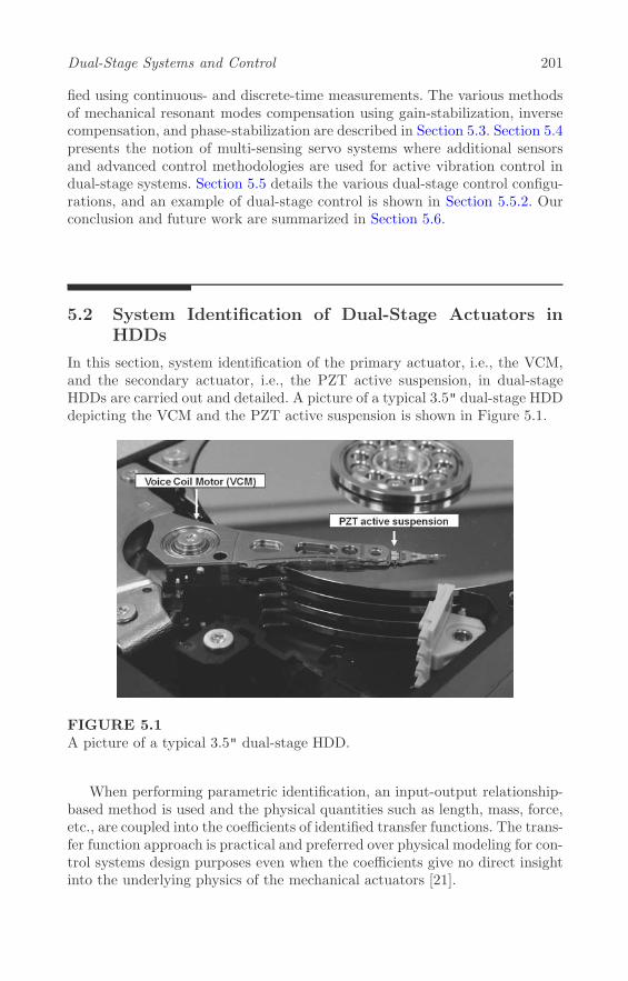
Dual-Stage Systems and Control 201
fied using continuous- and discrete-time measurements. The various methodsof mechanical resonant modes compensation using gain-stabilization, inversecompensation, and phase-stabilization are described in Section 5.3. Section 5.4presents the notion of multi-sensing servo systems where additional sensorsand advanced control methodologies are used for active vibration control indual-stage systems. Section 5.5 details the various dual-stage control configu-rations, and an example of dual-stage control is shown in Section 5.5.2. Ourconclusion and future work are summarized in Section 5.6.
5.2 System Identification of Dual-Stage Actuators inHDDs
In this section, system identification of the primary actuator, i.e., the VCM,and the secondary actuator, i.e., the PZT active suspension, in dual-stageHDDs are carried out and detailed. A picture of a typical 3.5" dual-stage HDDdepicting the VCM and the PZT active suspension is shown in Figure 5.1.
FIGURE 5.1A picture of a typical 3.5" dual-stage HDD.
When performing parametric identification, an input-output relationship-based method is used and the physical quantities such as length, mass, force,etc., are coupled into the coefficients of identified transfer functions. The trans-fer function approach is practical and preferred over physical modeling for con-trol systems design purposes even when the coefficients give no direct insightinto the underlying physics of the mechanical actuators [21].
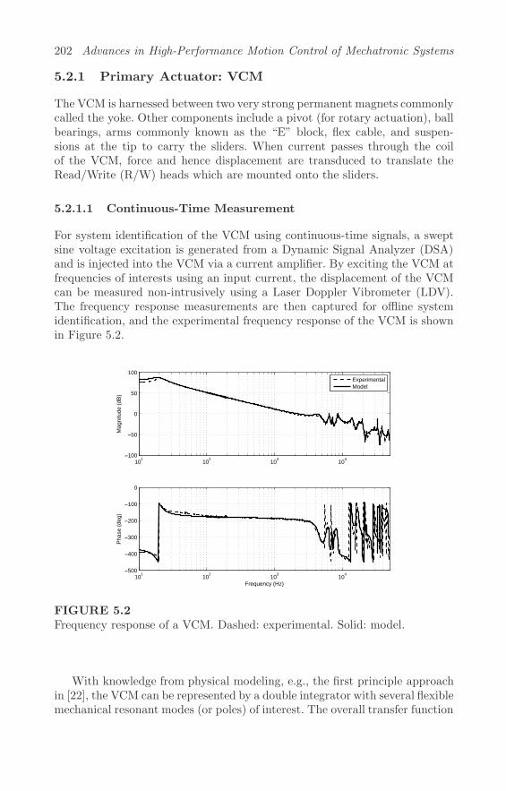
202 Advances in High-Performance Motion Control of Mechatronic Systems
5.2.1 Primary Actuator: VCM
The VCM is harnessed between two very strong permanent magnets commonlycalled the yoke. Other components include a pivot (for rotary actuation), ballbearings, arms commonly known as the “E” block, flex cable, and suspen-sions at the tip to carry the sliders. When current passes through the coilof the VCM, force and hence displacement are transduced to translate theRead/Write (R/W) heads which are mounted onto the sliders.
5.2.1.1 Continuous-Time Measurement
For system identification of the VCM using continuous-time signals, a sweptsine voltage excitation is generated from a Dynamic Signal Analyzer (DSA)and is injected into the VCM via a current amplifier. By exciting the VCM atfrequencies of interests using an input current, the displacement of the VCMcan be measured non-intrusively using a Laser Doppler Vibrometer (LDV).The frequency response measurements are then captured for offline systemidentification, and the experimental frequency response of the VCM is shownin Figure 5.2.
101 102 103 104−100
−50
0
50
100
Mag
nitu
de (d
B)
101 102 103 104−500
−400
−300
−200
−100
0
Phas
e (d
eg)
Frequency (Hz)
ExperimentalModel
FIGURE 5.2Frequency response of a VCM. Dashed: experimental. Solid: model.
With knowledge from physical modeling, e.g., the first principle approachin [22], the VCM can be represented by a double integrator with several flexiblemechanical resonant modes (or poles) of interest. The overall transfer function
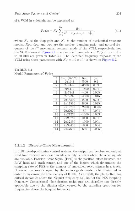
Dual-Stage Systems and Control 203
of a VCM in s-domain can be expressed as
PV (s) = KV
NV∑i=1
RV,is2 + 2ζV,iωV,is+ ω2
V,i
, (5.1)
where KV is the loop gain and NV is the number of mechanical resonantmodes. RV,i, ζV,i, and ωV,i are the residue, damping ratio, and natural fre-quency of the ith mechanical resonant mode of the VCM, respectively. Forthe VCM shown in Figure 5.1, the identified parameters of PV (s) from 10 Hzto 50 kHz are given in Table 5.1. The identified frequency response of theVCM using these parameters with KV = 1.9× 10⁴ is shown in Figure 5.2.
TABLE 5.1Modal Parameters of PV (s)
i ωV,i (rad/s) RV,i ζV,i1 2π19.5 7500 0.22 2π4449 –6500 0.093 2π6412 –1800 0.014 2π7141 –400 0.0055 2π8599 –4800 0.0156 2π13800 5500 0.027 2π17560 3800 0.0258 2π19750 –2400 0.00659 2π22620 50 0.00410 2π27270 –1300 0.00311 2π29780 1000 0.0112 2π32830 –1000 0.00113 2π38410 –800 0.00414 2π47610 650 0.005
5.2.1.2 Discrete-Time Measurement
In HDD head-positioning control systems, the output can be observed only atfixed time intervals as measurements can only be taken where the servo signalsare available. Position Error Signal (PES) is the position offset between theR/W head and track center, and one of the factors which determines thesampling rate of PES is the number of embedded servo signals in a track.However, the area occupied by the servo signals needs to be minimized inorder to maximize the areal density of HDDs. As a result, the plant often hascritical dynamics above the Nyquist frequency, i.e., half of the PES samplingfrequency. Conventional identification techniques are therefore not directlyapplicable due to the aliasing effect caused by the sampling operation forfrequencies above the Nyquist frequency.
204 Advances in High-Performance Motion Control of Mechatronic Systems
Although the LDV can also be used to measure the plant dynamics be-yond the Nyquist frequency using a similar methodology to that described inthe previous section, the displacement of the plant cannot be directly mea-sured after full assembly of the HDD. As such, it is imperative to develop amethod which can be carried out without external equipment for plant mea-surement and calibration of controller parameters in individual HDD unitsduring mass production. It is worth noting that the measurement and identi-fication methodology described in the previous section can be employed with-out distinguishing between continuous-time and discrete-time signals as well,if there are no significant dynamics beyond the Nyquist frequency.
In current literature, two kinds of non-parametric methods exist for identi-fication of HDD plant above the Nyquist frequency of the PES sampling rate.One method is to interpolate or interlace the measured plant response withanother measurement where the applied input excitation is shifted in time.Assuming the Linear Time-Invariant (LTI) property of the plant, the steady-state response of the plant for the time-shifted input excitation represents theplant response at sampling points equally shifted in time, if the sampling timeof the observation is not changed. By interpolating the frequency responses,the frequency response that is equivalent to the one measured at increasedsampling points can be reconstructed. The sampling rate of the measure-ments can be increased to arbitrarily high frequencies by reducing the sizeof the time shift and collecting as many measurements as necessary. The au-thors in [23] applied this principle to an HDD system using a discrete-timeexcitation signal. This approach can be used if the Digital-to-Analog (D/A)converter in the HDD is equipped with the functionality to shift its timingwith respect to the PES sampling operation.
The other method is to excite the plant by a single continuous-time sinu-soid. The method was developed by the authors in [24] to obtain the dynamicsof a continuous plant embedded in a closed-loop sampled-data system, and theHDD is mentioned as a possible application. Theoretically, one can obtain theplant dynamics up to arbitrarily high frequencies far beyond the Nyquist fre-quency of the PES. In practice, the continuous-time sinusoid can be replacedby a discrete-time sinusoid signal sampled at a frequency sufficiently higherthan the bandwidth of the plant as shown in [25]. Because of this approxima-tion, the frequency range for satisfactory measurement accuracy is limited bythe sampling rate of the discrete-time excitation signal.
In the following, a non-parametric method of identifying the plant dynam-ics above the Nyquist frequency based on [24] is presented. In the method, theapproximation required in [24] due to the infinite summation in computingthe transfer function is removed by directly measuring the sensitivity transferfunction of the feedback system in the discrete-time domain, using a discrete-time excitation signal instead of a continuous-time signal [25].
To investigate the effect of the sampling operation, the mathematical ex-pressions presented in [26] are briefly reviewed here. Sampling of a signal f(t)
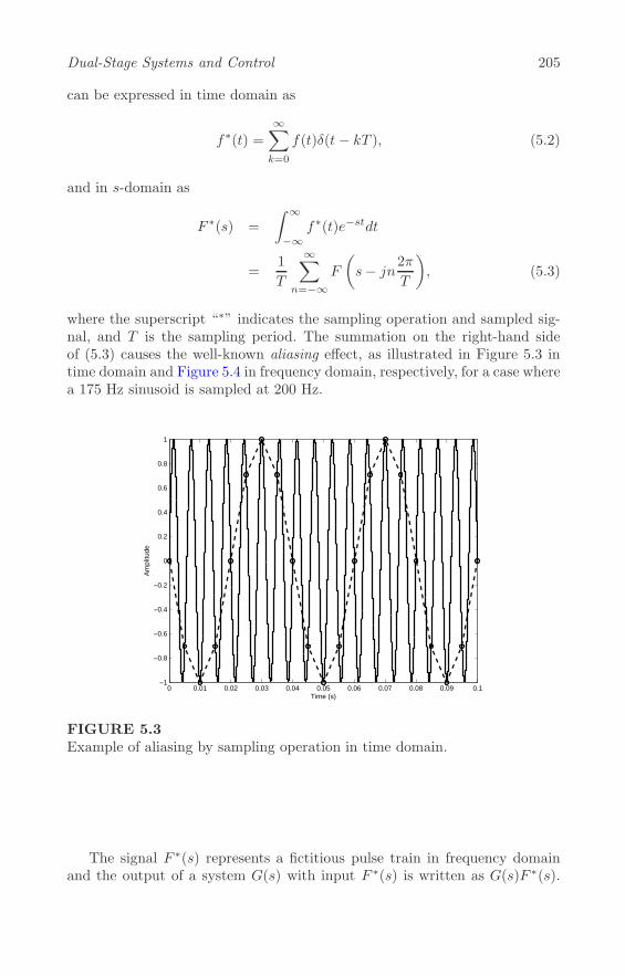
Dual-Stage Systems and Control 205
can be expressed in time domain as
f∗(t) =∞∑k=0
f(t)δ(t− kT ), (5.2)
and in s-domain as
F ∗(s) =
∫ ∞
−∞f∗(t)e−stdt
=1
T
∞∑n=−∞
F
(s− jn
2π
T
), (5.3)
where the superscript “∗” indicates the sampling operation and sampled sig-nal, and T is the sampling period. The summation on the right-hand sideof (5.3) causes the well-known aliasing effect, as illustrated in Figure 5.3 intime domain and Figure 5.4 in frequency domain, respectively, for a case wherea 175 Hz sinusoid is sampled at 200 Hz.
0 0.01 0.02 0.03 0.04 0.05 0.06 0.07 0.08 0.09 0.1−1
−0.8
−0.6
−0.4
−0.2
0
0.2
0.4
0.6
0.8
1
Time (s)
Ampl
itude
FIGURE 5.3Example of aliasing by sampling operation in time domain.
The signal F ∗(s) represents a fictitious pulse train in frequency domainand the output of a system G(s) with input F ∗(s) is written as G(s)F ∗(s).

206 Advances in High-Performance Motion Control of Mechatronic Systems
0 20 40 60 80 100 120 140 160 180 2000
0.2
0.4
0.6
0.8
1
Ampl
itude
0 20 40 60 80 100 120 140 160 180 2000
0.2
0.4
0.6
0.8
1
Frequency (Hz)
Ampl
itude
Continuous−time
Sampled−data
FIGURE 5.4Example of aliasing by sampling operation in frequency domain.
As the sampled signal F ∗(s) is periodic, sampling of this signal is expressedas
Y ∗(s) = [G(s)F ∗(s)]∗
= G∗(s)F ∗(s), (5.4)
since
[G(s)F ∗(s)]∗ =1
T
∞∑n=−∞
G
(s− jn
2π
T
)F ∗
(s− jn
2π
T
)
=
[1
T
∞∑n=−∞
G
(s− jn
2π
T
)]F ∗ (s)
= G∗(s)F ∗(s), (5.5)
provided that all sampling operations are synchronized.Using this property, the so-called pulse transfer function can be defined as
G∗(s) =Y ∗ (s)F ∗ (s)
=1
T
∞∑k=−∞
G
(s− jk
2π
T
). (5.6)
The pulse transfer function represents the relationship from the input pulsetrain to the output of the plant observed in continuous time. Although this
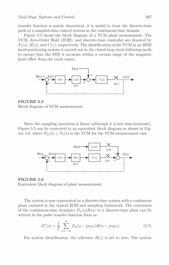
Dual-Stage Systems and Control 207
transfer function is purely theoretical, it is useful to treat the discrete-timepath of a sampled-data control system in the continuous-time domain.
Figure 5.5 shows the block diagram of a VCM plant measurement. TheVCM, Zero-Order Hold (ZOH), and discrete-time controller are denoted byP1(s), H(s), and C(z), respectively. The identification of the VCM in an HDDhead-positioning system is carried out in the closed-loop track-following modeto ensure that the PES is accurate within a certain range of the magnetichead offset from the track center.
( )D s
( )E z( )R z ( )Y z
FIGURE 5.5Block diagram of VCM measurement.
Since the sampling operation is linear (although it is not time-invariant),Figure 5.5 can be converted to an equivalent block diagram as shown in Fig-ure 5.6, where Pm(s) = P1(s) is the VCM for the VCM measurement case.
( )D s
( )E z( )R z ( )Y z
FIGURE 5.6Equivalent block diagram of plant measurement.
The system is now represented as a discrete-time system with a continuousplant enclosed in the typical ZOH and sampling framework. The conversionof the continuous-time dynamics Pm(s)H(s) to a discrete-time plant can bewritten in the pulse transfer function form as
G∗(s) =1
T
∞∑n=−∞
Pm(s− jnωT )H(s− jnωT ). (5.7)
For system identification, the reference R(z) is set to zero. The system

208 Advances in High-Performance Motion Control of Mechatronic Systems
output Y ∗(s) is the product of the discrete-time input, which is the sampledresponse of the plant Pm(s) subjected to a continuous-time excitation signalD(s), and the sensitivity transfer function of the discrete-time system writtenas
Y ∗(s) = S∗(s)[Pm(s)D(s)]∗. (5.8)
In (5.8), S∗(s) the sensitivity transfer function of the discrete-time feedbacksystem represented in a pulse transfer function form
S∗(s) =G∗(s)C∗(s)
1 +G∗(s)C∗(s). (5.9)
The frequency response of S∗(s) is periodic and can simply be obtained byevaluating Sd(e
jωT ) at ω, where Sd(z) is the discrete-time sensitivity transferfunction with z = ejwT . For measurement of the VCM, this includes the plantto be identified and therefore needs to be obtained experimentally by apply-ing a discrete-time excitation signal to the feedback system and measuringthe response of the sampled system. With Sd(e
jωT ), the sampled frequencyresponse of the plant subjected to an excitation signal D(jω) can be obtainedas
[Pm(jω)D(jω)]∗=
Y ∗(jω)Sd(ejωT )
. (5.10)
Since (5.10) is periodic with period 2πT , the plant response to a sinusoidal
excitation signal of frequency ωd can be obtained by (5.10) at frequency
ω′d = ωd − n
2π
T, (5.11)
where n ∈ Z+ is chosen such that 0 < ω′
d <2πT .
The frequency ωd of the excitation signal is not restricted by the samplingrate of the measurement, and the frequency response of the plant above theNyquist frequency of the sampling can be measured, except for frequenciesthat are integer multiples of 2π
T .Figure 5.7 shows the results of VCM plant identification obtained through
numerical simulations conducted with the models shown in Figure 5.5. Thesampling frequency of the PES measurement is 30 kHz, and the continuous-time VCM is simulated by a variable step solver with a maximum step sizeof 2.77 μs. In the simulation, the frequency response was measured for eachfixed continuous-time sinusoidal excitation signal varying from 50 Hz to 60 kHzat an interval of 50 Hz. The VCM model used is the 28th order model PV (s)identified previously in (5.1) with modal parameters in Table 5.1. It should benoted that the frequency responses at integer multiples of 2π
T are not plottedin Figure 5.7.

Dual-Stage Systems and Control 209
0 1 2 3 4 5 6x 10⁴
−150
−100
−50
0
50
Gai
n (d
B)
Plant ModelMeasurement
0 1 2 3 4 5 6x 10⁴
−150
−100
−50
0
50
100
150
Frequency (Hz)
Phas
e (d
eg)
FIGURE 5.7Frequency response measurement of VCM using PES sampled at 30 kHz.
In this example, the gain of the VCM controller C(z) is 0.1365. The loca-tions of the poles and zeros in discrete-time domain are shown in Table 5.2.
TABLE 5.2Parameters of VCM Controller C(z)
Order Zeros Poles1 −0.2199+ 0.9392i 0.00192 −0.2199− 0.9392i 0.0093 0.0741 + 0.9824i 0.50264 0.0741− 0.9824i 15 0.2163 + 0.9292i 0.0711 + 0.8581i6 0.2163− 0.9292i 0.0711− 0.8581i7 0.5777 + 0.7766i 0.2032 + 0.8504i8 0.5777− 0.7766i 0.2032− 0.8504i9 0.9896 + 0.0000i 0.5467 + 0.7287i10 0.9896− 0.0000i 0.5467− 0.7287i
In order to determine the frequency response of the continuous plant, thesensitivity transfer function Sd(e
jωT ) is measured by applying a discrete-timesinusoid from 50 Hz to 60 kHz sampled at 30 kHz as the continuous-timeexcitation signal through the ZOH. This is equivalent to Sd(e
jωT ) measuredup to 30 kHz and periodically extended up to 60 kHz.

210 Advances in High-Performance Motion Control of Mechatronic Systems
5.2.2 Secondary Actuator: PZT Active Suspension
To improve servo performance, the secondary actuator in a dual-stage systemshould be rigid (for higher damping and less number of mechanical resonantmodes) yet light (for achieving higher servo bandwidth) simultaneously. Sec-ondary actuators which possess these ideal characteristics can be used to rejectdisturbances in the control system for enhanced error correction in the highfrequency range.
In this section, system identification of a piezoelectric secondary actuatoror the PZT active suspension in a commercial dual-stage HDD is carried out.Two small parallel strips of PZT elements can be found at the base of thesuspension, and the piezoelectric ceramic PZT element has a high stiffnesswhich generates a large force by contraction and expansion. When a voltageis applied to these elements, one PZT strip expands while the other contractsto deflect the entire suspension and yields displacement of the R/W heads.PZT active suspensions often employ the push-pull or shear design accordingto the direction of polarization of the piezoelectric materials. Usually, the PZTactive suspension is designed to achieve a stroke of about 1 μm with the firstresonant mode in the range of 5–15 kHz. A picture of a two strip push-pullPZT active suspension is shown earlier in Figure 5.1.
5.2.2.1 Continuous-Time Measurement
Using the same methodology as the VCM case, the displacement of the PZTactive suspension is measured using the LDV. A swept sine voltage excita-tion is generated from a DSA at frequencies of interests, and is injected intothe PZT elements via a charge amplifier to reduce the effects of hysteresis.The frequency response measurements of the PZT active suspension are thencaptured for offline system identification as shown in Figure 5.8.
Figure 5.8 shows that the PZT active suspension can be modeled as a puregain in a large range of frequencies coupled with several high frequency me-chanical resonant modes. The transfer function of the PZT active suspensionPM (s) can be expressed in s-domain as
PM (s) = KM
NM∑i=1
RM,i
s2 + 2ζM,iωM,is+ ω2M,i
, (5.12)
where KM is the DC gain and NM is the number of mechanical resonantmodes of the PZT active suspension. RM,i, ζM,i, and ωM,i are the residue,damping ratio, and natural frequency of the ith mechanical resonant modeof the PZT active suspension, respectively. For the PZT active suspensionshown in Figure 5.1, the identified parameters of PM (s) from 10 Hz to 50 kHzare shown in Table 5.3. The identified frequency response of the PZT activesuspension using these parameters and KM = 0.3616 is shown in Figure 5.8.

Dual-Stage Systems and Control 211
101 102 103 104−60
−40
−20
0
20
Gai
n (d
B)
101 102 103 104−400
−300
−200
−100
0
Phas
e (d
eg)
Frequency (Hz)
ExperimentalModel
FIGURE 5.8Frequency response of PZT active suspension. Dashed: experimental. Solid:model.
TABLE 5.3Modal Parameters of PM (s)
i ωM,i (rad/s) RM,i(×108) ζM,i
1 2π2484 0.521 0.022 2π5461 2.005 0.0153 2π6074 2.206 0.014 2π9103 20.050 0.0125 2π12000 4.812 0.0156 2π14240 –7.218 0.0157 2π15830 –2.005 0.0158 2π18380 –5.213 0.0159 2π20000 –6.015 0.0210 2π23230 –4.010 0.0211 2π25300 –6.175 0.0212 2π30640 –5.213 0.0213 2π36000 2.566 0.01514 2π41280 –3.008 0.0215 2π48950 10.426 0.03
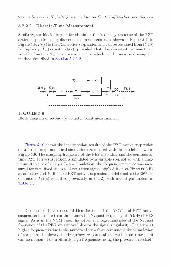
212 Advances in High-Performance Motion Control of Mechatronic Systems
5.2.2.2 Discrete-Time Measurement
Similarly, the block diagram for obtaining the frequency response of the PZTactive suspension using discrete-time measurements is shown in Figure 5.9. InFigure 5.9, P2(s) is the PZT active suspension and can be obtained from (5.10)by replacing Pm(s) with P2(s), provided that the discrete-time sensitivitytransfer function Sd(z) is known a priori, which can be measured using themethod described in Section 5.2.1.2.
( )D s
( )E z( )R z ( )Y z
FIGURE 5.9Block diagram of secondary actuator plant measurement.
Figure 5.10 shows the identification results of the PZT active suspensionobtained through numerical simulations conducted with the models shown inFigure 5.9. The sampling frequency of the PES is 30 kHz, and the continuous-time PZT active suspension is simulated by a variable step solver with a max-imum step size of 2.77 μs. In the simulation, the frequency response was mea-sured for each fixed sinusoidal excitation signal applied from 50 Hz to 60 kHzat an interval of 50 Hz. The PZT active suspension model used is the 30th or-der model PM (s) identified previously in (5.12) with modal parameters inTable 5.3.
Our results show successful identification of the VCM and PZT activesuspension for more than three times the Nyquist frequency of 15 kHz of PESsignal. As is in the VCM case, the values at integer multiples of the Nyquistfrequency of the PES are removed due to the signal singularity. The error athigher frequency is due to the numerical error from continuous-time simulationof the plant. In theory, the frequency response of the continuous-time plantcan be measured to arbitrarily high frequencies using the presented method.

Dual-Stage Systems and Control 213
0 1 2 3 4 5 6x 10⁴
−100
−50
0
50
Gai
n (d
B)
Plant modelMeasurement
0 1 2 3 4 5 6x 10⁴
−150
−100
−50
0
50
100
150
Frequency (Hz)
Phas
e (d
eg)
FIGURE 5.10Frequency response measurements of PZT active suspension using PES sam-pled at 30 kHz.
5.3 Resonance Compensation Without Extraneous Sen-sors
To improve the servo performance for next generation of high-performancemechatronic systems, the servo bandwidth needs to be further increased forenhanced positioning accuracy and speed. To achieve this, the servo loop needsto be carefully designed to take care of the disturbances (especially those atthe frequencies higher than the servo bandwidth) and should have enoughrobustness against gain and phase uncertainties. In particular, the open loopservo bandwidth should be designed at around one-third to one-quarter thefrequency of the first critical mechanical resonant mode as a rule of thumb [27].
In dual-stage HDDs, the existence of mechanical resonant modes in boththe VCM and PZT active suspension limits the increase of the gain crossoverfrequency as the gains of the actuators are usually very high at the resonantfrequencies and will degrade the closed-loop stability. As a result, the mechan-ical resonant modes excited by the air-flow would be mainly in the frequencyrange higher than the servo bandwidth, and the vibrations are amplified bythe mechanical resonant modes rather than being attenuated [28]. The largegains at the lightly damped poles not only cause oscillations in the step re-sponse, but even instability in the closed-loop servo system due to poor gainand phase margins. As such, several resonance compensation methods havebeen proposed to tackle these flexible resonant modes, and the commonly usedcontrol practices are presented in this section.

214 Advances in High-Performance Motion Control of Mechatronic Systems
5.3.1 Gain Stabilization
Gain stabilization is a technique used to suppress the energy (hence gain)of the mechanical resonant modes at the resonant frequencies by attenuatingthe signal power to avoid excitation of the corresponding resonant modes. Assuch, notch filters are commonly used to suppress the gain of the mechanicalresonant modes in the open loop transfer function [29]. Moreover, notch filtersare easy to design and implement in both continuous- and discrete-time, andare preferred over Low Pass Filters (LPFs) for their narrower band reductionin magnitude of gain at the resonant frequencies.
Suppose the ith mechanical resonant mode of a dual-stage actuator Ri(s)can be represented by
Ri(s) =(2πfR,i)
2
s2 + 2ζR,i(2πfR,i)s+ (2πfR,i)2, (5.13)
where fR,i and ζR,i are the natural frequency and damping ratio of the me-chanical resonant mode with (0 < ζR,i < 1). To cancel the gain of the me-chanical resonant mode, a straightforward notch filter designNi(s) for each i
th
resonant mode Ri(s) is
Ni(s) =(2πfD,i)
2
(2πfR,i)2s2 + 2ζR,i(2πfR,i)s+ (2πfR,i)
2
s2 + 2ζD,i(2πfD,i)s+ (2πfD,i)2. (5.14)
The damping ratio of the notch filter ζD,i is usually chosen to be√2 < ζD,i ≤ 1
to replace the lightly damped mechanical resonant modes with better dampedfilter poles. When fR,i = fD,i, some degradation in phase response is stillapparent at the resonant frequency fR,i. In this case, a high pass notch filterusing fD,i > fR,i can be constructed to reduce and even remove the phaseloss.
A setback of using notch filters is that they are not robust to paramet-ric variations, i.e., a shift in resonant frequencies might cause instability ofthe closed-loop system. Moreover, notch filters cannot completely reduce theresidual vibrations arising from the end of the track-seeking mode during modeswitching [30]. When the mechanical structural modes are excited by externaldisturbances, notch filters will also annihilate any control effort which is usedfor vibration damping [31].
5.3.2 Inverse Compensation
If the mechanical actuator contains minimum phase pole-zero pairs, a con-troller constructed by the approximated plant inverse can be used to makethe system behave as a rigid body up to high frequencies. This techniquenot only compensates for the large gain at the resonant modes, but also in-creases the gain of the anti-resonant zeros to reduce the signal blocking effectsof the anti-resonant zeros. This allows the actuator to be approximated by
Dual-Stage Systems and Control 215
the rigid-body mode for better error correction, especially at the frequen-cies of the anti-resonant zeros [32]. Moveover, inverse compensation reducesthe relative degree hence phase lag of the system up to high frequencies re-sulting in a higher servo bandwidth, which achieves a low positive gain ofthe sensitivity transfer function at high frequencies after the gain crossoverfrequency [33]. This resonance compensation phenomenon is also commonlyencountered when synthesizing H2 and H∞ optimal controllers.
However, a perfect plant inverse is not realizable in presence of unsta-ble zeros. As such, the effectiveness of the controller synthesized using theapproximated plant inverse will have to be carefully evaluated and substanti-ated. In particular, the Zero Phase Error Tracking (ZPET) controller [34] isa good candidate to achieve inverse compensation characteristics up to highfrequencies. Although the inverse compensation methodology does not appearto be robust against parametric perturbations and other uncertainties in themechanical actuator, the disturbance rejection capabilities and closed-loopstability are retained even when there is a ±5% shift in resonant frequenciesof the mechanical resonant modes [33].
5.3.3 Phase Stabilization
Contrary to gain stabilization or inverse compensation designs, the phase-stabilization design retains the high gain of the mechanical resonant mode butshapes the phase of the open loop transfer function to achieve closed-loop sta-bility. The phase-stabilization method involves designing lead compensatorsto lift the phase response of the open loop transfer function away from −180◦
to maintain stability. As such, the high loop gain at the resonant frequenciescan be maintained so that the sensitivity transfer function will have extra gainattenuation at the resonant frequencies, resulting in enhanced disturbance re-jection capabilities [22]. As the phase-stabilization methodology is achievedvia phase shaping, the technique is generally very robust if there are littlephase uncertainties in the mechanical actuator.
In the absence of mechanical resonant modes, LTI and Linear Time-Varying (LTV) peak filters can also be designed and included into the controlloop to emulate these desirable effects.
5.3.3.1 Using Mechanical Resonant Modes
The phase characteristics of the flexible resonant modes with respect to therigid body mode determines if the mechanical resonant modes are in-phase orout-of-phase. Besides performing modal analysis, this phase characteristic canalso be observed from the frequency response; a mechanical resonant modewhich is in-phase with the rigid body mode will exhibit a stable zero betweenthem, while a mechanical resonant mode which is out-of-phase with the rigidbody mode will exhibit an unstable zero between them.
The existence of in-phase mechanical resonant modes in actuators allows

216 Advances in High-Performance Motion Control of Mechatronic Systems
the phase-stabilization design to be achieved via low order controllers. Inthis design methodology, the notion of phase margins can be extended tosecond phase margin [35] or even tertiary phase margins [31] when multiple in-phase mechanical resonant modes exist. Interested readers are kindly referredto [22, 31, 35] for more details which are omitted here for brevity.
5.3.3.2 Using LTI Peak Filters
Peak filters with a high loop gain at its center frequency can also be used tocreate notches in the sensitivity transfer function to reject narrow frequencyband disturbances, similar to the advantages achieved via phase-stabilizedmechanical resonant modes. In general, it is preferable to augment the filtersinto the existing servo loop in an “add-on” fashion so that the design of eachloop can be decoupled [36]. In [37, 38], the add-on filters were placed at thedisturbance frequencies where there were no significant plant dynamics, i.e.,lightly damped plant poles. The phase stabilizability can be guaranteed byappropriately placing a zero so that the closed-loop is robust against phaseuncertainties around the disturbance frequency [39, 40]. In other cases, thepoles of the peak filter should be placed near some lightly damped plantpoles. In this case, setting the damping of the peak filter as that of the plantpoles which are within the bandwidth of the filter could be a compromisemade between performance and stability as shown in [39, 41].
In this section, novel solutions are provided for designing the disturbancefilter when significant plant dynamics are within the bandwidth of the peakfilter. The filter zero is designed appropriately so that the root loci originatingfrom both the filter poles and lightly damped plant poles enter the left-halfplane under certain low gain conditions. As such, the departure angles fromthe filter poles are no longer 180◦ but ±90◦, i.e., compromised departure anglesfrom both the filter poles and plant poles. By doing so, the stability marginespecially the gain margin is dramatically increased [42]. The resulting closed-loop systems can provide large gain attenuation, i.e., disturbance rejectioncapability at the disturbance frequency.
A peak filter is augmented into the existing servo loop in an add-on fashionas shown in Figure 5.11, where P (s), C(s), and F (s) are the plant, baselinecontroller, and disturbance filter, respectively. d, y, and r denote the outputdisturbance, plant output, and reference signal, respectively.
F
C P
d
+++++
_r y
FIGURE 5.11Block diagram of control system with an add-on peak filter.

Dual-Stage Systems and Control 217
The overall sensitivity transfer function S(s) can be given by
S(s) = S0(s)SF (s), (5.15)
where S0(s)=1
1+P (s)C(s) is the baseline sensitivity transfer function,
i.e., S(s) = S0(s) when F (s) = 0, and SF (s) can be expressed as
SF (s) =1
1 + Sh(s)F (s), (5.16)
where Sh(s)=P (s)C(s)
1+P (s)C(s) is the baseline complimentary sensitivity transfer
function. From (5.15), it can be seen that the design of baseline servo loopand the peak filter can be decoupled [36]. The baseline controller C(s) takescare of the plant P (s) to guarantee the basic stability margin, while the peakfilter F (s) takes care of the pseudo “plant” Sh(s) so that the resulting SF (s)has desired attenuation at those disturbance frequencies.
Two kinds of plant models will be considered; namely, one without signif-icant plant dynamics within the bandwidth of the peak filter followed by theother with them. The peak filter F (s) is given in the form of
F (s) = Ks(s cosϕ+ ω1 sinϕ)
s2 + 2ζ1ω1s+ ω21
, (5.17)
where K>0 is the gain of the filter and can be chosen by means of root locusanalysis to guarantee closed-loop stability. In particular, one zero of F (s)is placed at the origin to maintain a low gain in the frequency range lowerthan the disturbance frequency so that the effect of the peak filter F (s) tothe baseline servo loop can be minimized at the frequencies other than thedisturbance frequency. The other zero will be placed optimally so that theroot loci of Sh(s)F (s) originating from the poles associated with F (s) willmove in the most stable direction [40]
ϕ = arg[Sh(jω1)] +π
2, ϕ ∈ [−π
2,π
2]. (5.18)
An illustration example is shown in Figures 5.12 and 5.13. Figure 5.12 plotsthe root loci of Sh(s)F (s), where the solid and dashed line are the root lociassociated with the filter and pseudo plant, respectively. It can be seen thatthe angles of departure from the complex conjugate poles of F (s) are 180◦
as depicted by the solid line in Figure 5.12, which gives a most stable phasemargin of ±90◦.
Define the pseudo open loop transfer function G(s) as
G(s) = Sh(s)F (s), (5.19)
the phase at the disturbance frequency can be calculated by
arg[G(jω1)] = arg[Sh(jω1)] + arg[F (jω1)]. (5.20)

218 Advances in High-Performance Motion Control of Mechatronic Systems
−1 −0.5 0 0.5 1 1.5 2
x 105
−4
−3
−2
−1
0
1
2
3
4x 10⁵
Real
Imag
inar
y
−3 −2.5 −2 −1.5 −1 −0.5 0 0.5 1 1.5
x 104
−1
−0.8
−0.6
−0.4
−0.2
0
0.2
0.4
0.6
0.8
1x 10⁵
Real
Imag
inar
y
Departure angle=180o
Gain margin=�
Departure angle=180o
Gain margin=13.1
FIGURE 5.12Root loci of Sh(s)F (s). Solid: filter pole. Dashed: plant pole.
−3 −2 −1 0 1 2−2.5
−2
−1.5
−1
−0.5
0
0.5
1
1.5
2
2.5
Real
Imag
inar
y
103 104−14
−12
−10
−8
−6
−4
−2
0
2
Frequency (Hz)
Gai
n (d
B)
−1 circle
Nominal open loop P(s)C(s)
Overall open loop P(s)C(s)[1+F(s)]
Gain attenuation
(a) (b)
FIGURE 5.13(a) Nyquist plot of the open loop system; (b) Magnitude of sensitivity transferfunction of the closed-loop system. Solid: without F (s). Dashed: with F (s).
Noting arg[F (jω1)] = arctan( cosϕsinϕ ) and from (5.18), it follows that
arg[G(jω1)] = arg[Sh(jω1)] + arctan{− tan
[arg[Sh(jω1)]
]}= 0. (5.21)
In addition, the relationship among the transfer functions of the overall re-sulting open loop, baseline open loop, and pseudo open loop is
P (s)C(s)[1 + F (s)] = [1 + P (s)C(s)][1 + Sh(s)F (s)]− 1. (5.22)
If there are no significant plant dynamics near the disturbance frequency andthe disturbance frequency is much higher than the servo bandwidth, i.e.,the contribution of gain and phase of the nominal open loop P (s)C(s) to
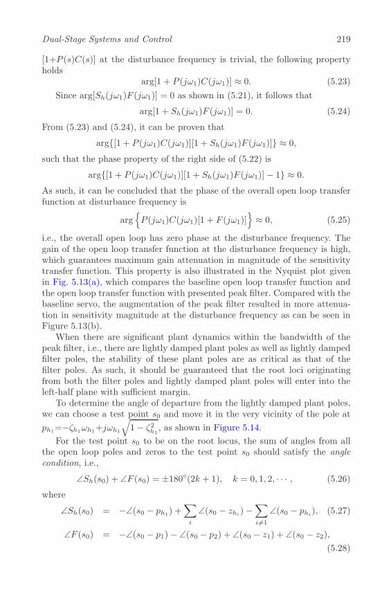
Dual-Stage Systems and Control 219
[1+P (s)C(s)] at the disturbance frequency is trivial, the following propertyholds
arg[1 + P (jω1)C(jω1)] ≈ 0. (5.23)
Since arg[Sh(jω1)F (jω1)] = 0 as shown in (5.21), it follows that
arg[1 + Sh(jω1)F (jω1)] = 0. (5.24)
From (5.23) and (5.24), it can be proven that
arg{[1 + P (jω1)C(jω1)][1 + Sh(jω1)F (jω1)]} ≈ 0,
such that the phase property of the right side of (5.22) is
arg{[1 + P (jω1)C(jω1)][1 + Sh(jω1)F (jω1)]− 1} ≈ 0.
As such, it can be concluded that the phase of the overall open loop transferfunction at disturbance frequency is
arg{P (jω1)C(jω1)[1 + F (jω1)]
}≈ 0, (5.25)
i.e., the overall open loop has zero phase at the disturbance frequency. Thegain of the open loop transfer function at the disturbance frequency is high,which guarantees maximum gain attenuation in magnitude of the sensitivitytransfer function. This property is also illustrated in the Nyquist plot givenin Fig. 5.13(a), which compares the baseline open loop transfer function andthe open loop transfer function with presented peak filter. Compared with thebaseline servo, the augmentation of the peak filter resulted in more attenua-tion in sensitivity magnitude at the disturbance frequency as can be seen inFigure 5.13(b).
When there are significant plant dynamics within the bandwidth of thepeak filter, i.e., there are lightly damped plant poles as well as lightly dampedfilter poles, the stability of these plant poles are as critical as that of thefilter poles. As such, it should be guaranteed that the root loci originatingfrom both the filter poles and lightly damped plant poles will enter into theleft-half plane with sufficient margin.
To determine the angle of departure from the lightly damped plant poles,we can choose a test point s0 and move it in the very vicinity of the pole at
ph1=−ζh1ωh1+jωh1
√1− ζ2h1
, as shown in Figure 5.14.
For the test point s0 to be on the root locus, the sum of angles from allthe open loop poles and zeros to the test point s0 should satisfy the anglecondition, i.e.,
∠Sh(s0) + ∠F (s0) = ±180◦(2k + 1), k = 0, 1, 2, · · · , (5.26)
where
∠Sh(s0) = −∠(s0 − ph1) +∑i
∠(s0 − zhi)−∑i�=1
∠(s0 − phi), (5.27)
∠F (s0) = −∠(s0 − p1)− ∠(s0 − p2) + ∠(s0 − z1) + ∠(s0 − z2),
(5.28)

220 Advances in High-Performance Motion Control of Mechatronic Systems
*
Re
Im s0
z1 z2
1hp dep,1h�
1� 2�
1�
2�
2p
1p
FIGURE 5.14Determination of angle of departure from a plant pole. “o”: zeros z1 and z2of F (s). “x”: poles p1 and p2 of F (s). “*”: pole of the plant.
with zhi and phi being the zeros and poles of the plant, respectively. z1=0,z2=−ω1 tanϕ, and p1,2 = −ζ1ω1 ± jω1
√1− ζ21 are the zeros and poles of the
peak filter, respectively.The angle of departure from the plant pole at ph1 is defined as the angle
from ph1 to the test point s0, i.e.,
φh1,dep = ∠(s0 − ph1). (5.29)
As ph1 , p1, and p2 are lightly damped poles, i.e., they are very close to theimaginary axis and s0 is in the very vicinity of ph1 , the following approxima-tions hold
∠(s0 − p2) ≈ ∠(ph1 − p2) ≈ ∠(p1 − p2) = 90◦, (5.30)
∠(s0 − z1) ≈ ∠(ph1 − z1) ≈ 90◦, (5.31)
∠(s0 − z2) ≈ ∠(ph1 − z2) ≈ ∠(p1 − z2) = 90◦ − ϕ. (5.32)
If ϕ is given by (5.18), i.e.,
ϕ =∑i
∠(jω1 − zhi)−∑i
∠(jω1 − phi) + 90◦, (5.33)
the following approximation can be obtained by noting that the point jω1 isvery close to p1, ph1 , and s0 with
∑i
∠(jω1 − zhi) ≈∑i
∠(s0 − zhi). (5.34)

Dual-Stage Systems and Control 221
In addition, the sum of the angle from jω1 to all the plant poles except thepole at ph1 can also be approximated by
∑i�=1
∠(jω1 − phi) ≈∑i�=1
∠(s0 − phi). (5.35)
As such, it can be concluded from (5.26)–(5.35) that
−φh1,dep − ∠(s0 − p1) + ∠(jω1 − ph1) = ±180◦(2k + 1). (5.36)
In Figure 5.15, we define φ1 = ∠(s0 − p1) and θ0 = ∠(jω1 − ph1). Theresonant frequency in the closed-loop (i.e., the pseudo-plant) will be slightlypushed down and the damping ratio will be smaller when there is no loop-shaping for the resonant mode. This makes the pole of the pseudo-plant atph1 lower than the resonant frequency in the complex s-plane. On the otherhand, the imaginary part of the pole at p1 will be almost equivalent to thatof jω1 if the damping ratio ζ1 is very small. The resulting layout of p1, ph1 ,and jω1 is depicted in Figure 5.15(a).
Re
Im
s0 1hp
1p 1�j1�
dep,1h� 0�
Re
Im
s0 1hp 1p
1�j
o01 =� dep,1h�0�
(a) (b)
* *
FIGURE 5.15Relationship of angles: (a) phase-shift method; (b) frequency-shift method.
Under this framework and for the resonance located at a very high fre-quency range especially those above 10 kHz, φ1 ≈ ∠(ph1 −p1) ≈ (−75◦,−90◦)and θ0 ≈ (75◦, 90◦). From (5.36) it can be concluded that the angle of depar-ture from the plant pole at ph1 is
φh1,dep = 360◦k, k = 0, 1, 2, · · · , (5.37)
which means that the plant poles will enter into the right-half plane undera very small gain margin. The closed-loop system will then be considered asunstable.
An example which has a resonant mode at 12 kHz and a damping ratio
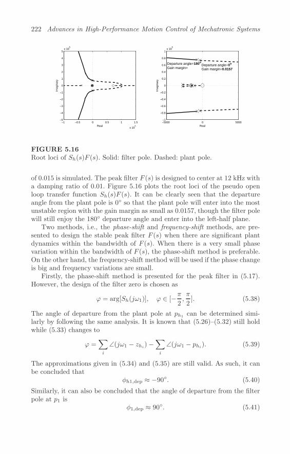
222 Advances in High-Performance Motion Control of Mechatronic Systems
−1 −0.5 0 0.5 1 1.5
x 105
−5
−4
−3
−2
−1
0
1
2
3
4
5x 10⁵
Real
Imag
inar
y
−5000 0 5000−1
−0.8
−0.6
−0.4
−0.2
0
0.2
0.4
0.6
0.8
1x 10⁵
Real
Imag
inar
y
Departure angle=180o Gain margin=�
Departure angle=0o
Gain margin=0.0157
FIGURE 5.16Root loci of Sh(s)F (s). Solid: filter pole. Dashed: plant pole.
of 0.015 is simulated. The peak filter F (s) is designed to center at 12 kHz witha damping ratio of 0.01. Figure 5.16 plots the root loci of the pseudo openloop transfer function Sh(s)F (s). It can be clearly seen that the departureangle from the plant pole is 0◦ so that the plant pole will enter into the mostunstable region with the gain margin as small as 0.0157, though the filter polewill still enjoy the 180◦ departure angle and enter into the left-half plane.
Two methods, i.e., the phase-shift and frequency-shift methods, are pre-sented to design the stable peak filter F (s) when there are significant plantdynamics within the bandwidth of F (s). When there is a very small phasevariation within the bandwidth of F (s), the phase-shift method is preferable.On the other hand, the frequency-shift method will be used if the phase changeis big and frequency variations are small.
Firstly, the phase-shift method is presented for the peak filter in (5.17).However, the design of the filter zero is chosen as
ϕ = arg[Sh(jω1)], ϕ ∈ [−π2,π
2]. (5.38)
The angle of departure from the plant pole at ph1 can be determined simi-larly by following the same analysis. It is known that (5.26)–(5.32) still holdwhile (5.33) changes to
ϕ =∑i
∠(jω1 − zhi)−∑i
∠(jω1 − phi). (5.39)
The approximations given in (5.34) and (5.35) are still valid. As such, it canbe concluded that
φh1,dep ≈ −90◦. (5.40)
Similarly, it can also be concluded that the angle of departure from the filterpole at p1 is
φ1,dep ≈ 90◦. (5.41)
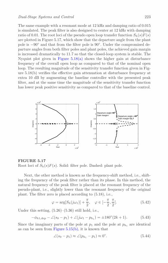
Dual-Stage Systems and Control 223
The same example with a resonant mode at 12 kHz and damping ratio of 0.015is simulated. The peak filter is also designed to center at 12 kHz with dampingratio of 0.01. The root loci of the pseudo open loop transfer function Sh(s)F (s)are plotted in Figure 5.17, which show that the departure angle from the plantpole is −90◦ and that from the filter pole is 90◦. Under the compromised de-parture angles from both filter poles and plant poles, the achieved gain marginis increased dramatically to 11.7 so that the closed-loop system is stable. TheNyquist plot given in Figure 5.18(a) shows the higher gain at disturbancefrequency of the overall open loop as compared to that of the nominal openloop. The resulting magnitude of the sensitivity transfer function given in Fig-ure 5.18(b) verifies the effective gain attenuation at disturbance frequency atextra 10 dB by augmenting the baseline controller with the presented peakfilter, and at the same time the magnitude of the sensitivity transfer functionhas lower peak positive sensitivity as compared to that of the baseline control.
−6 −4 −2 0 2
x 104
−8
−6
−4
−2
0
2
4
6
8x 10⁵
Real
Imag
inar
y
−2 −1 0 1 2
x 104
−2
−1.5
−1
−0.5
0
0.5
1
1.5
2x 10⁵
Real
Imag
inar
y
Departure angle=90o Gain margin=� Departure angle=−90o
Gain margin=11.7
FIGURE 5.17Root loci of Sh(s)F (s). Solid: filter pole. Dashed: plant pole.
Next, the other method is known as the frequency-shift method, i.e., shift-ing the frequency of the peak filter rather than its phase. In this method, thenatural frequency of the peak filter is placed at the resonant frequency of thepseudo-plant, i.e., slightly lower than the resonant frequency of the originalplant. The filter zero is placed according to (5.18), i.e.,
ϕ = arg[Sh(jω1)] +π
2, ϕ ∈ [−π
2,π
2]. (5.42)
Under this setting, (5.26)–(5.36) still hold, i.e.,
−φh1,dep − ∠(s0 − p1) + ∠(jω1 − ph1) = ±180◦(2k + 1). (5.43)
Since the imaginary parts of the pole at p1 and the pole at ph1 are identicalas can be seen from Figure 5.15(b), it is known that
∠(s0 − p1) ≈ ∠(ph1 − p1) ≈ 0◦. (5.44)

224 Advances in High-Performance Motion Control of Mechatronic Systems
−4 −3 −2 −1 0 1 2 3 4−3
−2
−1
0
1
2
3
4
Real
Imag
inar
y
104−15
−10
−5
0
5
10
15
Frequency (Hz)
Gai
n (d
B)
−1 circle
Gain attenuation
Nominal open loop P(s)C(s)
Overall open loop P(s)C(s)[1+F(s)]
(a) (b)
FIGURE 5.18(a) Nyquist plot of the open loop system; (b) Magnitude of the sensitivitytransfer function of the closed-loop system. Solid: with F (s). Dashed: with-out F (s).
As such, the angle of departure from the pole at ph1 is
φh1,dep ≈ ±90◦. (5.45)
The angle of departure from the filter pole at p1 can also be similarly approx-imated by
φ1,dep ≈ ±90◦. (5.46)
The same example with a resonant mode at 12 kHz and damping ratiobeing 0.015 is simulated. The peak filter is designed to center slightly lowerat 11.8 kHz with a damping ratio 0.01. The root loci of the pseudo openloop Sh(s)F (s) are plotted in Figure 5.19, which shows that the departureangle from the plant pole is −90◦ and that from the filter pole is 90◦. Underthese compromised departure angles from both filter poles and plant poles, theachieved gain margin is increased dramatically to 8.22 so that the closed-loopsystem is stable. The Nyquist plot given in Figure 5.20(a) shows the highergain at disturbance frequency of the overall open loop transfer function ascompared to that of the nominal open loop transfer function. The resultingmagnitude of the sensitivity transfer function given in Figure 5.20(b) verifiesthe effective gain attenuation at disturbance frequency with an extra 8 dBby augmenting the baseline controller with the presented peak filter, and atthe same time the magnitude of sensitivity transfer function has a lower peakpositive sensitivity as compared to the baseline control.
5.3.3.3 Using LTV Peak Filters
In addition to the amount of gain attenuation, the duration of the tran-sient response is the other critical design factor when designing peak filters.

Dual-Stage Systems and Control 225
−6 −4 −2 0 2
x 104
−8
−6
−4
−2
0
2
4
6
8x 10⁵
Real
Imag
inar
y
−2 −1 0 1 2
x 104
−1.5
−1
−0.5
0
0.5
1
1.5x 10⁵
Real
Imag
inar
y
Departure angle=90o Gain margin=�
Departure angle=−90o
Gain margin=8.22
FIGURE 5.19Root loci of Sh(s)F (s). Solid: filter pole. Dashed: plant pole.
−4 −3 −2 −1 0 1 2 3 4−3
−2
−1
0
1
2
3
4
Real
Imag
inar
y
104−15
−10
−5
0
5
10
15
Frequency (Hz)
Gai
n (d
B)
−1 circle
Overall open loop P(s)C(s)[1+F(s)]
Nominal open loop P(s)C(s)
Gain attenuation
(a) (b)
FIGURE 5.20(a) Nyquist plot of the open loop system; (b) Magnitude of the sensitivitytransfer function of the closed-loop system. Solid: with F (s). Dashed: with-out F (s).
However, these two design factors are contradictory to each other. Usually, atrade-off exists between the transient response and the bandwidth of the gainnotch [43, 44, 45]. The simultaneous improvement for transient response intime-domain and gain attenuation in frequency-domain could be very hard toachieve for conventional LTI filters. As such, Linear Time-Varying (LTV) fil-ters have been proposed in [46] and [47] with varying filter gain and dampingratio (or quality factor Q in communications and filter engineering).
In this section, a peak filtering scheme with improved transient responseis presented using the same peak filter structure in (5.17). The properties ofthe LTV peak filters are (i) the gain and the damping ratio of the filter are

226 Advances in High-Performance Motion Control of Mechatronic Systems
adjusted along the time to ensure faster attenuation in time-domain and widerbandwidth in the frequency-domain, (ii) the stability during the transientperiod is guaranteed by taking into account the poles of the lightly dampedplant as critical poles, and ensuring the root loci originating from these polesenter into the left-half plane through placing the filter zero properly, and(iii) during steady-state, both filter poles and plant poles should be takeninto account so that compromised departure angles from both filter poles andplant poles are adopted to ensure closed-loop stability [48].
In the transient stage, the width of the disturbance rejection band shallbe large to ensure faster attenuation. As such, the gain and damping ratio ofthe peak filter should be large and their values should be scheduled to reducealong the time as
θ(t) = θ[d− (d− 1)h(t)], (5.47)
where θ=K or ζ1, d=θ(0)/θ defines the variation range of θ(t), andh(t) describes the step response of a supportive system H(s), i.e.,h(t)=L−1{s−1H(s)} where L−1 is the inverse Laplace transform operator.For our design, H(s) is chosen as a first-order system as
H(s) =γ
s+ γ, γ > 0. (5.48)
In this case, 0 < θ < θ(0) is the lower bound of θ(t) so that θ(t) decreases inthe variation interval for d > 1. As such, (5.47) can be rewritten as
θ(t) = θ
[1 +
(θ(0)
θ− 1
)e−γt
], (5.49)
or in discrete-time as
θ(kTs) = θ
[1 +
(θ(0)
θ− 1
)e−γkTs
], (5.50)
with Ts being the step size for parametric updates.The initial value of the damping ratio can be chosen such that the poles of
the resulting filter are well-damped to ensure stability of the lightly dampedplant poles which are comparatively more critical. The lower bound of thedamping ratio is chosen to achieve the desired width of attenuation. To guar-antee the closed-loop stability for the transient stage, the root loci originatingfrom the lightly damped plant poles should enter into the left-half plane. Thefilter zero is placed according to
ϕ = arg[Sh(jω1)] + π, ϕ ∈ [−π2,π
2]. (5.51)
Similarly, the angle of departure from the plant poles is
φp,dep ≈ −180◦, (5.52)

Dual-Stage Systems and Control 227
and the angle of departure from the filter poles is
φf,dep ≈ 0◦. (5.53)
In the steady-state stage, the lower bound for the parameter tuning θ willbe adopted and fixed for the peak filter.
Due to the small damping ratio, stability of the resulting lightly dampedfilter poles is as critical as that of the plant poles. As such, the root locioriginating from both the filter poles and the plant poles should enter into theleft-half plane. The scheme of compromised departure angles similar to theLTI peak filter case in the previous section will be adopted here such that theangles of departure from the filter poles and the plant poles are
φp,dep ≈ ±90◦, (5.54)
and
φf,dep ≈ ∓90◦. (5.55)
A simple example is given here to illustrate and showcase the effectivenessof the presented method. A second-order system with a low frequency modeat 50 Hz and damping ratio of 0.4 plus a resonant mode at 12 kHz anddamping ratio of 0.015 is used. The peak filter is designed to center at 12kHz. The initial values of the parameter tuning in transient stage are chosenas K(0) = 1, ζ1(0) = 0.1, and the lower bounds are K = 0.2, ζ1 = 0.02, andγ = 3000.
The root loci of the open loop at the initial stage are plotted in Figure5.21, where it can be seen that the departure angle from a plant pole is −180◦
and that from a filter pole is 0◦. The gain margin of the plant pole is 108 whilethe gain margin of the filter pole is infinity. Figure 5.22 plots the root loci ofthe open loop at steady-state. By providing the compromised departure anglesfor both filter poles and plant poles, which are 90◦ and −90◦, respectively, theachieved gain margin is sufficiently large as infinity and 16, respectively.
The stability margins of the closed-loop systems during both transientand steady-state stages are improved using the presented add-on LTI andLTV peak filters with improved transient responses.
5.3.4 Experimental Verifications
In this section, the phase-stabilization method of resonance compensationusing mechanical resonant modes, LTI peak filters, and LTV peak filters areverified with simulations and experiments on a VCM-actuated arm in a typicalmechatronic system. In the experiments, the LDV is used to measure thelateral displacement of the VCM-actuated arm, and our presented controlalgorithms are implemented on dSPACE at a sampling frequency of 30 kHz.The frequency responses of the open loop and sensitivity transfer functionsare shown in Figures 5.23 and 5.24, respectively.

228 Advances in High-Performance Motion Control of Mechatronic Systems
−3 −2 −1 0 1 2
x 104
5
5.5
6
6.5
7
7.5
8
8.5
9
9.5
10x 104
Real
Imag
inar
y
−2 −1 0 1 2
x 105
−2
−1.5
−1
−0.5
0
0.5
1
1.5
2x 10⁵
Real
Imag
inar
yDeparture angle=−180o
Gain margin=108
Departure angle=0o Gain margin=�
FIGURE 5.21Root loci and angles of departure. Solid: filter pole. Dashed: plant pole.
−3 −2 −1 0 1 2
x 104
5
5.5
6
6.5
7
7.5
8
8.5
9
9.5
10x 104
Real
Imag
inar
y
−2 −1 0 1 2
x 105
−2
−1.5
−1
−0.5
0
0.5
1
1.5
2x 10⁵
Real
Imag
inar
y
Departure angle=90o Gain margin=�
Departure angle=−90o Gain margin=16
FIGURE 5.22Root loci and angles of departure. Solid: filter pole. Dashed: plant pole.
From Figure 5.23, it can be seen that the in-phase mechanical resonantmode at 5161 Hz has been phase-stabilized, while the out-of-phase resonantmode at 7913 Hz has been reshaped to be in-phase with the rigid body modeusing the presented resonance compensation methods with peak filters. As aresult, an attenuation gain of more than 12 dB can be observed at 5161 Hzand 7913 Hz in the magnitudes of the sensitivity transfer functions as shownin Figure 5.24, which greatly improve the disturbance rejection capabilities atboth resonant frequencies.
The transient performance is evaluated and compared between peak fil-ters with time-varying parameters using a look-up table and time-invariantparameters via simulations. Firstly, a set of gain and damping ratio valuesis obtained to reshape the critical mechanical resonant mode at 7913 Hz to

Dual-Stage Systems and Control 229
103 104−40
−30
−20
−10
0
10
20
Mag
nitu
de (d
B)
103 104−1500
−1000
−500
0
Phas
e (d
eg)
Frequency (Hz)
With peak filterWithout peak filter
FIGURE 5.23Frequency responses of open loop transfer functions.
103 104−20
−15
−10
−5
0
5
10
Mag
nitu
de (d
B)
Frequency (Hz)
With peak filterWithout peak filter
FIGURE 5.24Frequency responses of sensitivity transfer functions.
be in-phase, and are chosen as their steady-state values. Secondly, the initialvalues of the gain and damping ratio are chosen to be relatively larger thantheir steady-state values. Thirdly, the gain Kf and damping ratio ζ of the
230 Advances in High-Performance Motion Control of Mechatronic Systems
peak filter are updated using
θ(t)=θs
[1+
(θiθs
)e−γt
], (5.56)
where γ>0 is the decaying rate of the parameters. θi and θs are the initialand steady-state values of the gain or damping ratio, respectively. A sinusoidalsignal of 7913 Hz with unity amplitude is used as the output disturbance toevaluate the transient performances of the two schemes with no measurementnoise included. The LTV peak filter with initial and steady-state values of(Kf , ζ)=(2, 0.1) → (0.5, 0.01) shows improved transient performance over theLTI peak filter as shown in Figure 5.25.
0 0.5 1 1.5 2 2.5 3 3.5 4 4.5 5x 10⁻³
−1
−0.8
−0.6
−0.4
−0.2
0
0.2
0.4
0.6
0.8
1
Time (s)
PES
(�m
)
LTI filterLTV filter
FIGURE 5.25Transient performances of presented LTV and LTI peak filters.
5.4 Resonance Compensation With Extraneous Sensors
In dual-stage servo systems, it is common that the combined output remainsas the only available feedback signal even when there are two mechanical actu-ators to be precisely controlled. With the improvements in disturbance rejec-tion performance by incorporation of extraneous sensors and active-sensingmethodologies, the feasibility of employing multi-sensing servo systems [49]through enhanced sensor fusion in mechatronic systems have been studied. Re-cently, advances in piezoelectric materials also allow self-sensing servo systems
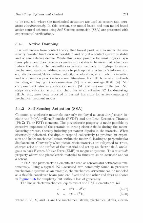
Dual-Stage Systems and Control 231
to be realized, where the mechanical actuators are used as sensors and actu-ators simultaneously. In this section, the model-based and non-model-basedactive control schemes using Self-Sensing Actuation (SSA) are presented withexperimental verifications.
5.4.1 Active Damping
It is well known from control theory that lowest positive area under the sen-sitivity transfer function is achievable if and only if a control system is stableand of zero relative degree. While this is not possible for most physical sys-tems, placement of extra sensors ensure more states to be measured, which canreduce the order of the controllers as in state feedback. In high-performancemechatronic systems, adding sensors to pick up extra actuator’s information,e.g., displacement/deformation, velocity, acceleration, strain, etc., is intuitiveand is a common practice in current literature. For HDDs, several methodsincluding employing (i) accelerometers [50] in a single-stage HDD, (ii) PZTcompound actuator as a vibration sensor [51] and (iii) one of the two PZTstrips as a vibration sensor and the other as an actuator [52] for dual-stageHDDs, etc., have been reported in current literature for active damping ofmechanical resonant modes.
5.4.2 Self-Sensing Actuation (SSA)
Common piezoelectric materials currently employed as actuators/sensors in-clude the PolyVinylDeneFlouride (PVDF) and the Lead-Zirconate-Titanate(Pb-Zr-Ti, or PZT) elements. The piezoelectric property is made possible byexcessive exposure of the ceramic to strong electric fields during the manu-facturing process, thereby inducing permanent dipoles in the material. Whenelectrically polarized, the dipoles respond collectively to produce an expan-sion and hence mechanical strain within the material, leading to perpendiculardisplacement. Conversely when piezoelectric materials are subjected to strain,charges arise on the surface of the material and set up an electric field, analo-gous to back Electro-Motive Force (EMF) in magnetic systems. This reversibleproperty allows the piezoelectric material to function as an actuator and/ora sensor.
In SSA, the piezoelectric elements are used as sensors and actuators simul-taneously. Using a typical PZT-actuated arm commonly found in precisionmechatronic systems as an example, the mechanical structure can be modeledas a flexible cantilever beam (one end fixed and the other end free) as shownin Figure 5.26 for simplicity but without loss of generality.
The linear electromechanical equations of the PZT elements are [53]
S = sET + dTE, (5.57)
D = dT + εTE, (5.58)
where S, T , E, and D are the mechanical strain, mechanical stress, electri-
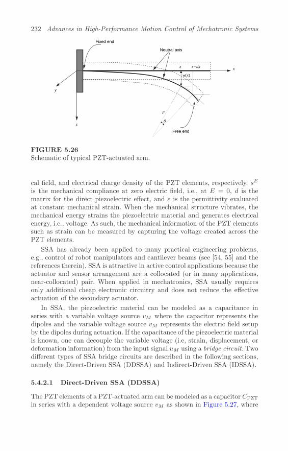
232 Advances in High-Performance Motion Control of Mechatronic Systems
x
z
y
Neutral axis
w(x)
x x+dx
ρ
θ
Fixed end
Free end
FIGURE 5.26Schematic of typical PZT-actuated arm.
cal field, and electrical charge density of the PZT elements, respectively. sE
is the mechanical compliance at zero electric field, i.e., at E = 0, d is thematrix for the direct piezoelectric effect, and ε is the permittivity evaluatedat constant mechanical strain. When the mechanical structure vibrates, themechanical energy strains the piezoelectric material and generates electricalenergy, i.e., voltage. As such, the mechanical information of the PZT elementssuch as strain can be measured by capturing the voltage created across thePZT elements.
SSA has already been applied to many practical engineering problems,e.g., control of robot manipulators and cantilever beams (see [54, 55] and thereferences therein). SSA is attractive in active control applications because theactuator and sensor arrangement are a collocated (or in many applications,near-collocated) pair. When applied in mechatronics, SSA usually requiresonly additional cheap electronic circuitry and does not reduce the effectiveactuation of the secondary actuator.
In SSA, the piezoelectric material can be modeled as a capacitance inseries with a variable voltage source vM where the capacitor represents thedipoles and the variable voltage source vM represents the electric field setupby the dipoles during actuation. If the capacitance of the piezoelectric materialis known, one can decouple the variable voltage (i.e, strain, displacement, ordeformation information) from the input signal uM using a bridge circuit. Twodifferent types of SSA bridge circuits are described in the following sections,namely the Direct-Driven SSA (DDSSA) and Indirect-Driven SSA (IDSSA).
5.4.2.1 Direct-Driven SSA (DDSSA)
The PZT elements of a PZT-actuated arm can be modeled as a capacitor CPZT
in series with a dependent voltage source vM as shown in Figure 5.27, where

Dual-Stage Systems and Control 233
a Direct-Driven SSA (DDSSA) scheme is employed as the input signal uM isapplied across the entire bridge circuit.
uM
vM
R1 C1 R3
C2
+_v1
v2 vs
Differential amplifierCPZT
C3
FIGURE 5.27Direct-Driven SSA bridge circuit.
In Figure 5.27, resistors R1 and R3 are sometimes placed in parallel withcapacitors C1 and C3 to prevent DC drifts, and the values of capacitors C1, C2,and C3 are to be determined. When the bridge circuit is subjected to inputvoltage uM , the PZT-actuated arm is transduced to give displacement yM . Thevoltage vM generated is hence proportional to yM (arising from mechanicalstrain) of the PZT-actuated arm, and can be be decoupled from uM using adifferential amplifier. From Figure 5.27, the following equations hold
v1 =CPZT
C1 + CPZT(uM − vM ), (5.59)
v2 =C2
C2 + C3uM , (5.60)
vs = v2 − v1
=
(CPZT
C1 + CPZT− C2
C2 + C3
)uM +
CPZT
C1 + CPZTvM . (5.61)
By measuring CPZT a priori and ensuring that capacitors C1 = C2 =C3 = CPZT, the bridge circuit is balanced. A PZT-actuated arm displacementestimator is established as
vs =CPZT
C1 + CPZTvM
=vM2. (5.62)
As such, vM is decoupled from the input signal uM and can be used for ac-tive control purposes. The only trade-off when driving the PZT-actuated armand the bridge circuit directly using the input signal uM is that a larger uM

234 Advances in High-Performance Motion Control of Mechatronic Systems
is needed for the same amount of required displacement yM as compared tothat without the bridge circuit [54]. This loads the input signal uM , and canbe alleviated by using the Indirect-Driven SSA (IDSSA) bridge circuit.
5.4.2.2 Indirect-Driven SSA (IDSSA)
In the Indirect-Driven SSA (IDSSA) circuit as shown in Figure 5.28, addi-tional capacitors and resistors are required in the feedback loops of opera-tional amplifiers so that the circuit acts as a high-pass filter after differentialamplification. This results in better self-sensing performance for higher Signal-to-Noise Ratio (SNR) measurements and wider sensing bandwidth to detecthigh frequency mechanical resonant modes in the PZT-actuated arm.
+_
+_
vM
+_
+_
v1
v2
CPZT
PZTC
C1
C2
C3
C4R3
R2
R4
R1
R5
R6
R3R8
uM vs
FIGURE 5.28Indirect-Driven SSA bridge circuit.
The sensing voltage vM generated from the strain of the PZT element canbe decoupled from uM as shown in the following derivations. The Laplacetransform of v1(t) and v2(t) can be derived as
v1(s) =
[1 +
C1CPZTR1R2s2 + C1R2s
C1C2R1R2s2 + (CPZT + C1 + C2)R1s+ 1
]uM (s)
− (CPZT/C2)s2
s2 + (CPZT + C1 + C2)s/C1C2R2 + (1/C1C2R1R2)vM (s),
v2(s) =
[1 +
C3C′PZTR3R4s
2 + C3R4s
C3C4R3R4s2 + (C ′PZT + C3 + C4)R1s+ 1
]uM (s), (5.63)
and the output of the IDSSA bridge circuit vS(s) is given by
vS(s) =R6
R5 +R6
R7 +R8
R8v2(s)− R7
R8v1(s). (5.64)
In this case, the components in Figure 5.28 are chosen to be⎧⎪⎪⎨⎪⎪⎩
C1 = C2 = C3 = C4 = C′PZT = CPZT,
R1 = R2 = R3 = R4,R5 = R8,R6 = R7 = kR5,
(5.65)

Dual-Stage Systems and Control 235
the bridge circuit is balanced and vM (s) is similarly decoupled from uM (s)with
vS(s)
vM (s)=
ks2
s2 + 2ζ(2πfc)s+ (2πfc)2, (5.66)
where fc=1
2π√C1C2R1R2
, ζ=√C1C2R1R2(C1+C2+CPZT)
2C1C2R2, and k are the cut-off fre-
quency, damping ratio, and gain of the high-pass filter, respectively. The com-ponents of resistors and capacitors in Figure 5.28 are chosen depending onthe desired corner frequency of the high-pass filter and sensing bandwidthaccordingly.
With the presented SSA bridge circuits, inner loop control methodologiescan be developed to stiffen the PZT-actuated arm via active damping beforethe entire outer dual-stage control loop is closed. The model-based and non-model-based designs are described in the following sections for inner loopdamping of the mechanical resonant modes in the PZT-actuated arm. For therest of the chapter, a sampler is used in the place of the ZOH H(s) in allcontrol block diagrams for brevity but without loss of generality.
5.4.3 Model-Based Design
In this section, the model-based resonance compensation design using SSA isdescribed in detail. The model-based SSA control topology with the ActiveMode Damping (AMD) controller CD is shown in Figure 5.29.
PMuD
yM
CD1
BH HB
uM
vs
+–
*My
FIGURE 5.29Model-based SSA control topology.
In Figure 5.29, the estimated displacement of the PZT-actuated arm y∗Mis obtained from SSA for feedback control. The digital inverse of displacementestimation circuit H−1
B (z) is designed from the dynamics of the displacementestimation circuit HB. H
−1B (z) is required to obtain a real time estimated y∗M
for the AMD controller CD to damp the PZT-actuated arm’s sway modesusing inner loop compensation, with possible attenuation of the torsion modeswhich was previously impossible if y∗M using SSA was unavailable [54].
The PZT-actuated arm displacement estimation circuit HB consists of thePZT-actuated arm/sensor and a differential amplifier. As vM (hence vs) inFigures 5.27 and 5.28 arises from yM , HB should be modeled by a transfer

236 Advances in High-Performance Motion Control of Mechatronic Systems
function HB(s) = vs(s)yM (s) . A digital inverse of HB(s), H
−1B (z), is constructed
to provide an estimate of the displacement of the PZT-actuated arm y∗M . Asaturation function is also included to take into account the saturation of thePZT-actuated arm as shown in Figure 5.29.
Using SSA, the collocation of the PZT-actuated arm and the PZT-actuatedarm’s displacement sensor is nearly achieved. As such, a robust AMD con-troller for damping the PZT-actuated arm’s mechanical resonant modes canbe designed, and the AMD controller CD,i(s) for each i
th mechanical resonantmode is given by
CD,i(s) = KD,i
s+ωn,i
εi
s+κiωn,i
εi
s+ ωn,is+
εiωn,i
κi
, (5.67)
to increase the damping ratios (hence reduced gains) of the PZT-actuatedarm’s torsion modes and sway modes. KD,i is set to εi in most cases. εiand κi are tuning parameters, and 1 < εi ≤ P is chosen usually for robustnessagainst natural frequency variations P % (P < 3 for most physical systems).5 < κi < 15 is then chosen to determine the amount of phase lift required tostabilize the resonant mode at the natural frequency ωn,i.
The overall AMD controller CD can be obtained from the product CD,i(s)for the total number of torsion and sway modes to be damped. Phase leadcompensators are sometimes added to reduce the phase loss introduced bythe AMD controllers and to increase the gain of the PZT-actuated arm’sdisplacement for high frequency mode detection. In essence, CD is a generalcase of traditional Positive Position Feedback (PPF) vibration controllers [56]with additional zeros. The zeros prevent causality issues in PPF arrangements,and improve the stability margin of the closed-loop system. The presentedAMD controller increases the gain of each resonant mode and stabilizes thecontrol loop using a phase lead from the zeros at
ωn,i
εi, which is a common result
when using optimal control methods such as H∞ loop shaping techniques.
Assuming the PZT-actuated arm PM has resonant modes at natural fre-quencies ωn,i and the AMD controller CD in (5.67) is included in a negativefeedback configuration as shown in Figure 5.29. The following closed-loopequation holds
yM (s)
uM (s)=
PM (s)
1 + CD(s)PM (s), (5.68)
if the closed-loop system is stable. As such, the gains of the mechanical reso-nant modes are suppressed by the AMD controller at the frequencies ωn,i of

Dual-Stage Systems and Control 237
the modes effectively by a factor of 1|CD(jωn,i)| as
∣∣∣∣yM (jωn,i)
uM (jωn,i)
∣∣∣∣ =
∣∣∣∣PM (jωn,i)
1 + CD(jωn,i)PM (jωn,i)
∣∣∣∣
≈ |PM (jωn,i)||CD(jωn,i)PM (jωn,i)|
=1
|CD(jωn,i)| , (5.69)
if |CD(jωn,i)PM (jωn,i)| >> 1.
To illustrate the effectiveness of the presented scheme on PZT-actuatedarms in precision mechatronic systems, a PZT active suspension in a com-mercial dual-stage HDD is modeled as PM (s) and identified to have torsionmodes at 4.31 kHz and 6.52 kHz, a bending mode at 11.04 kHz, and a swaymode at 21.08 kHz [54]. The simulated frequency responses of the presentedAMD controller CD(s) and the open loop transfer function CD(s)PM (s) areshown in Figure 5.30.
102 103 104−40
−20
0
20
40
Mag
nitu
de (d
B)
102 103 104−200
−150
−100
−50
0
50
100
150
Phas
e (d
eg)
Frequency (Hz)
AMD controllerOpen loop
FIGURE 5.30Simulated frequency responses. Solid: AMD controller CD(s). Dotted: openloop transfer function CD(s)PM (s).
With CD(s) in the feedback path as shown in Figure 5.29 and (5.67), theloop is closed to damp the PZT active suspensions’s torsion modes and swaymode. The experimental frequency responses of the PZT active suspensionwith and without the presented AMD controller CD are shown in Figure 5.31.It can be seen from Figure 5.31 that the PZT active suspension’s torsion modes

238 Advances in High-Performance Motion Control of Mechatronic Systems
at 4.31 kHz and 6.52 kHz (about 5 dB) as well as sway mode at 21.08 kHz(about 30 dB) are all damped by the AMD controller CD.
102 103 104−60
−40
−20
0
20G
ain
(dB)
102 103 104−1000
−800
−600
−400
−200
0
200
Frequency (Hz)
Phas
e (d
eg)
Without proposed AMD controllerWith proposed AMD controller
FIGURE 5.31Experimental frequency responses of PZT active suspension. Solid: withoutAMD controller CD. Dashed-dot: with AMD controller CD.
The presented AMD controller CD using the model-based design is moreeffective in suppressing the sway modes as compared to the torsion modes(and bending modes). This is obvious as the estimated PZT-actuated arm’sdisplacement y∗M from the displacement estimation circuit HB is only effectivein measuring in-plane components (making the in-plane sway modes observ-able and controllable) of the PZT-actuated arm and not the torsion modes(out-of-plane weakly controllable modes). This is unavoidable as the PZT-actuated arm’s displacement estimation circuit HB produces a scalar signaland the PZT-actuated arm has more degrees of freedom than control inputs,i.e., under-actuation.
5.4.4 Non-Model-Based Design
Rather than directly feeding back the strain signal from SSA, an adaptivenon-model-based control scheme is used to enhance the performance of vibra-tion suppression. In this section, the structure of the PZT-actuated arm isanalyzed, followed by the adaptive algorithm and its stability proof [57].
Assume that the cross-section of the suspension is a symmetrical area (iny−z plane) which is perpendicular to the neutral plane (in x−z plane) asshown earlier in Figure 5.26. When deformed in the x − z plane with the x-
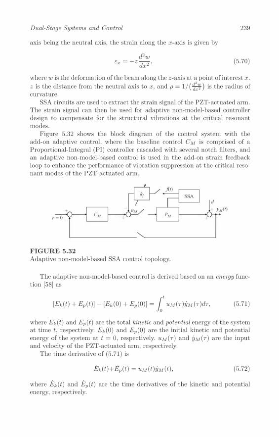
Dual-Stage Systems and Control 239
axis being the neutral axis, the strain along the x-axis is given by
εx = −z d2w
dx2, (5.70)
where w is the deformation of the beam along the z-axis at a point of interest x.
z is the distance from the neutral axis to x, and ρ = 1/(d2wdx2
)is the radius of
curvature.SSA circuits are used to extract the strain signal of the PZT-actuated arm.
The strain signal can then be used for adaptive non-model-based controllerdesign to compensate for the structural vibrations at the critical resonantmodes.
Figure 5.32 shows the block diagram of the control system with theadd-on adaptive control, where the baseline control CM is comprised of aProportional-Integral (PI) controller cascaded with several notch filters, andan adaptive non-model-based control is used in the add-on strain feedbackloop to enhance the performance of vibration suppression at the critical reso-nant modes of the PZT-actuated arm.
FIGURE 5.32Adaptive non-model-based SSA control topology.
The adaptive non-model-based control is derived based on an energy func-tion [58] as
[Ek(t) + Ep(t)]− [Ek(0) + Ep(0)] =
∫ t
0
uM (τ)yM (τ)dτ, (5.71)
where Ek(t) and Ep(t) are the total kinetic and potential energy of the systemat time t, respectively. Ek(0) and Ep(0) are the initial kinetic and potentialenergy of the system at t = 0, respectively. uM (τ) and yM (τ) are the inputand velocity of the PZT-actuated arm, respectively.
The time derivative of (5.71) is
Ek(t)+Ep(t) = uM (t)yM (t), (5.72)
where Ek(t) and Ep(t) are the time derivatives of the kinetic and potentialenergy, respectively.

240 Advances in High-Performance Motion Control of Mechatronic Systems
The adaptive non-model-based control uM (t) is designed as the combina-tion of a PI control and an adaptive strain feedback term, which is expressedas
uM (t) = −kpyM (t)− ki
∫ t
0
yM (τ)dτ − kff(t)
∫ t
0
f(τ)dτ, (5.73)
where kp and ki> 0 are proportional and integral gains, respectively. f(t) is asignal reflecting the deformation of the controlled plant, e.g., the strain, whichshould be chosen such that it is zero when the controlled plant is static withoutdeformation. The gain kf>0 is for the add-on strain feedback loop, where alarger kf leads to faster transient performance but undesired high-gain controland more energy consumption, and vice versa.
An adaptive tuning for kf can be achieved by setting kf=Y2s (t), and Ys(t)
is updated by
Ys(t) = αYs(t)yM (t)f(t)
∫ t
0
f(τ)dτ − βYs(t), (5.74)
where α>0 sets the updating rate. β>0 is introduced to avoid divergence of theintegral gains in the presence of various disturbances and plant uncertainties.With β, Ys(t) acts as a first order filter of αYs(t)yM (t)f(t)
∫ t0f(τ)dτ thus
guaranteeing convergence.Note that PI control is used in (5.73) rather than PD control in [58]. The
integral term is used to eliminate the steady-state error. To accommodate theextra term, the integral gain is chosen as ki=k
20(t), where k0(t) is adaptively
tuned by
k0(t) = γk0(t)yM (t)
∫ t
0
yM (τ)dτ, (5.75)
where γ>0 sets the updating rate of k0(t).The stability of the closed-loop system with the add-on adaptive control
is proven as follows. The Lyapunov function candidate is chosen as
V (t) = Ek(t) + Ep(t) +1
2kpy
2M (t) +
1
2α−1Y 2
s (t) +1
2γ−1k20(t). (5.76)
Using (5.72), the time derivative of V (t) is
V (t) = uM (t)yM (t) + kpyM (t)yM (t) + α−1Ys(t)Ys(t) + γ−1k0(t)k0(t). (5.77)
Substituting (5.73)–(5.75) into (5.77) yields
V (t) =[− kpyM (t)− ki
∫ t
0
yM (τ)dτ − kff(t)
∫ t
0
f(τ)dτ]yM (t)
+α−1Ys(t)[αYs(t)yM (t)f(t)
∫ t
0
f(τ)dτ − βYs(t)]
+kpyM (t)yM (t) + k20(t)yM (t)
∫ t
0
yM (τ)dτ
= −α−1βY 2s (t) ≤ 0, (5.78)

Dual-Stage Systems and Control 241
102 103 104
−40
−20
0
20
40
Gai
n (d
B)
102 103 104−800
−600
−400
−200
0
200
Phas
e (d
eg)
Frequency (Hz)
Open loopPlant model
FIGURE 5.33Frequency responses of open loop transfer functions. Dashed: plant model.Solid: open loop.
which is negative semi-definite, i.e., the closed-loop system is energy dissipativeand stable. Since the stability condition in (5.78) is independent of systemdynamics, the control system is robust against plant uncertainties.
The effectiveness of the presented scheme on PZT-actuated arms is evalu-ated with experiments on a PZT active suspension in a commercial dual-stageHDD. From Figure 5.33, it can be seen that the PZT active suspension hasresonant modes at 5.4 kHz, 16 kHz, 20.9 kHz, and 25.6 kHz. A PI controller inseries with four notch filters at these natural frequencies is used as the baselinecontroller CM . The frequency response of the open loop transfer function isshown in Figure 5.33, and a gain crossover frequency of about 1.5 kHz withsufficient gain margin and phase margins are achieved.
To explore the effects of the adaptive non-model-based control in the fre-quency range of interests, the amplitudes of the sensitivity transfer functionswith and without the presented adaptive non-model-based control are plottedin Figure 5.34. Note that the sensitivity transfer function with the adaptivenon-model-based control is measured at steady-state, i.e., after the adapta-tion has converged at each frequency. Figure 5.34 shows a 50% and 75% im-provements in vibration suppression capabilities at critical resonant modesat 5.4 kHz and 21 kHz when using the presented adaptive non-model-basedcontrol with SSA.
In the mass production of PZT-actuated arms for mechatronic systems, sig-nificant amount of parametric perturbations exist in the natural frequencies,damping ratios, and residues of the critical resonant modes. The presentedadaptive non-model-based control with SSA is more robust against paramet-ric perturbations as the strain signal is proportional to the mechanical de-
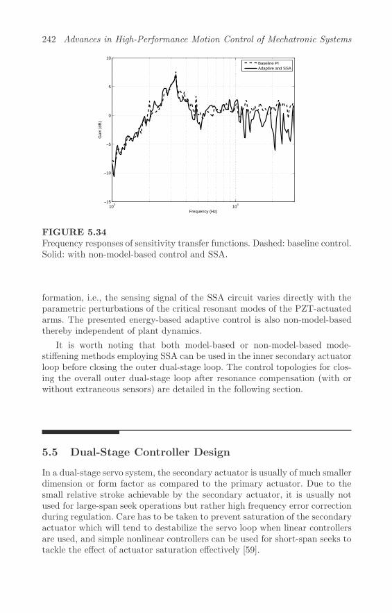
242 Advances in High-Performance Motion Control of Mechatronic Systems
103 104−15
−10
−5
0
5
10
Frequency (Hz)
Gai
n (d
B)
Baseline PIAdaptive and SSA
FIGURE 5.34Frequency responses of sensitivity transfer functions. Dashed: baseline control.Solid: with non-model-based control and SSA.
formation, i.e., the sensing signal of the SSA circuit varies directly with theparametric perturbations of the critical resonant modes of the PZT-actuatedarms. The presented energy-based adaptive control is also non-model-basedthereby independent of plant dynamics.
It is worth noting that both model-based or non-model-based mode-stiffening methods employing SSA can be used in the inner secondary actuatorloop before closing the outer dual-stage loop. The control topologies for clos-ing the overall outer dual-stage loop after resonance compensation (with orwithout extraneous sensors) are detailed in the following section.
5.5 Dual-Stage Controller Design
In a dual-stage servo system, the secondary actuator is usually of much smallerdimension or form factor as compared to the primary actuator. Due to thesmall relative stroke achievable by the secondary actuator, it is usually notused for large-span seek operations but rather high frequency error correctionduring regulation. Care has to be taken to prevent saturation of the secondaryactuator which will tend to destabilize the servo loop when linear controllersare used, and simple nonlinear controllers can be used for short-span seeks totackle the effect of actuator saturation effectively [59].

Dual-Stage Systems and Control 243
5.5.1 Control Structure
Three common control structures, i.e., the parallel, Coupled Master-Slave(CMS), and Decoupled Master-Slave (DMS), will be described in this sec-tion. It is assumed that the resonance compensation methods described in theprevious section are used for both the primary and secondary actuators, andare included in the corresponding controllers accordingly a priori.
Assuming the following nomenclature with PV being the primary actuatorand PM as the secondary actuator, CV being the primary actuator controllerand CM as the secondary actuator controller. Define LD as the open looptransfer function and TD = LD
1+LDas the complementary sensitivity trans-
fer function (or closed-loop transfer function) of the dual-stage control loop.Define SV = 1
1+CV PV, SM = 1
1+CMPM, and SD = 1
1+LDas the sensitivity
transfer functions of the primary actuator loop, secondary actuator loop, andoverall dual-stage control loop, respectively. Define eV and eM as the errorsignals, uV and uM as the control signals, yV and yM as the displacements,where the subscripts V and M indicate the primary and secondary loop, re-spectively. Define r as the reference and y as the output of the dual-stageservo system. Note that the effects of disturbances and noises are omitted inthe following block diagrams.
5.5.1.1 Parallel
As there are two actuators to be controlled in a dual-stage servo system, thefollowing Dual-Input-Single-Output (DISO) parallel control structure is in-tuitive. The functional block diagram of the parallel structure is shown inFigure 5.35, where the corresponding open loop, sensitivity, and complemen-tary sensitivity transfer functions of the parallel configuration are
LD = CV PV + CMPM , (5.79)
SD =1
1 + CV PV + CMPM, (5.80)
TD =CV PV + CMPM
1 + CV PV + CMPM. (5.81)
From (5.79), it can be seen that the gain crossover frequency of the dual-stage control loop is higher than that when using single-stage actuation solely.This can be achieved when the phase of the CV PV and CMPM are approxi-mately equal at the gain crossover frequency. In addition, the sensitivity func-tion has an addition of CMPM in the denominator as can be seen from (5.80),resulting in more effective disturbance suppression and rejection in the dual-stage control loop. Controller designs using the parallel structure usually resultin |CV PV | � |CMPM | in the low frequency range and |CV PV | � |CMPM |in the high frequency range. This frequency allocation allows the secondaryactuator to reject disturbances in the high frequency range, while the primaryactuator functions in the low frequencies for error correction.

244 Advances in High-Performance Motion Control of Mechatronic Systems
PM
CV PV+
++
_r y
CM
ev
eM
uv
uM
yv
yM
FIGURE 5.35Parallel configuration.
Among the various works on HDD dual-stage servo control using the par-allel configuration, the authors proposed the so-called PQ method in [60]. ThePQ method is a systematic procedure that simplifies the DISO control systeminto a fictitious Single-Input-Single-Output (SISO) control system for succes-sive loop closures design in the frequency domain, and interested readers arereferred to [60] for more details.
5.5.1.2 Coupled Master-Slave (CMS)
The primary advantage of a master-slave configuration is to have priorityonto one actuator over the other [61], making the secondary actuator respondfaster to external disturbances by being the “master” and the bulkier primaryactuator as the “slave” to compensate for slower variations in the relativedisplacement between the actuators.
The master-slave configuration comes in a slight variation, namely theCoupled Master-Slave (CMS) and the Decoupled Master-Slave (DMS) controlstructure. Both configurations require a secondary actuator model P ∗
M to es-timate the output of the secondary actuator y∗M which is fed to the primaryactuator controller CV . The functional block diagram of the CMS configura-tion is shown in Figure 5.36.
PM
CV PV+
++
_r y
eM
uv
uM
yv
yMCM
*MP
uM
*My
ev
FIGURE 5.36Coupled master-slave configuration.
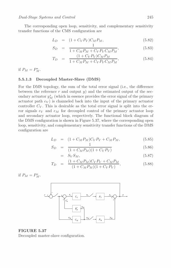
Dual-Stage Systems and Control 245
The corresponding open loop, sensitivity, and complementary sensitivitytransfer functions of the CMS configuration are
LD = (1 + CV PV )CMPM , (5.82)
SD =1
1 + CMPM + CV PV CMPM, (5.83)
TD =(1 + CV PV )CMPM
1 + CMPM + CV PV CMPM, (5.84)
if PM = P ∗M .
5.5.1.3 Decoupled Master-Slave (DMS)
For the DMS topology, the sum of the total error signal (i.e., the differencebetween the reference r and output y) and the estimated output of the sec-ondary actuator y∗M (which in essence provides the error signal of the primaryactuator path eV ) is channeled back into the input of the primary actuatorcontroller CV . This is desirable as the total error signal is split into the er-ror signals eV and eM for decoupled control of the primary actuator loopand secondary actuator loop, respectively. The functional block diagram ofthe DMS configuration is shown in Figure 5.37, where the corresponding openloop, sensitivity, and complementary sensitivity transfer functions of the DMSconfiguration are
LD = (1 + CMPM )CV PV + CMPM , (5.85)
SD =1
(1 + CMPM )(1 + CV PV )(5.86)
= SV SM , (5.87)
TD =(1 + CMPM )CV PV + CMPM(1 + CMPM )(1 + CV PV )
, (5.88)
if PM = P ∗M .
PM
CV PV+
++
_r y
eM
uv
uM
yv
yMCM
*MP
uM
*My
ev+
+
FIGURE 5.37Decoupled master-slave configuration.
246 Advances in High-Performance Motion Control of Mechatronic Systems
Note that the sensitivity transfer function of the DMS structure is theproduct of the sensitivity transfer functions of the primary actuator and thesecondary actuator loop, hence decoupled. Obviously, the DMS design canbe converted into the parallel design when the new primary actuator CV P isdesigned as
CV P = (1 + CMPM )CV . (5.89)
Using the DMS control structure, controller design and implementationwill be eased as the loops can be designed independently and dual-stage closed-loop stability will be ensured if the primary and secondary actuator loops arestable. Moreover, enhanced disturbance rejection can be ensured via sensitiv-ity transfer function loop shaping independently, since the overall dual-stagesensitivity transfer function SD is the product of the sensitivity functions inthe individual paths. The authors in [35] designed a phase-stable controller forthe PZT active suspension using the proposed second phase margin index toretain the large gain of the resonant poles for notches in the sensitivity trans-fer function. In [33], the authors proposed a Near Perfect Modeling (NPM)method to construct a virtual PZT actuated active suspension digital modelinverse to reduce the positive gain of the dual-stage sensitivity transfer func-tion using Discrete Bode’s Integral Theorem.
The performances of the CMS and DMS configuration depend highly onthe effectiveness of the secondary actuator estimator P ∗
M . If the estimatorprovides a fairly accurate estimation, i.e., yM ≈ y∗M , the expected disturbancerejection capabilities and servo performance can be achieved as a good esti-mate of the error eV in the primary actuator loop is available for decouplingcontrol. These can be achieved in some cases, e.g., using SSA on piezoelectric-driven secondary actuators [54] as described in the previous section.
5.5.2 Design Example
In this section, the dual-stage controller design methodologies are illustratedon a commercial dual-stage HDD using a DMS configuration for simplicitybut without loss of generality. In a dual-stage HDD using the PZT activesuspension as the secondary actuator, only the relative displacement of theR/W head or PES is available. With the DMS configuration, controller designis usually carried out on the VCM and PZT active suspension loop separatelyand then combined into a complete dual-stage loop. This method gives actualinsight into the working principles of the two actuators at different frequencyranges, and different control topologies will be discussed in this section.
Due to the limited displacement range of the PZT active suspension, theactuation effort between the two actuators should be distributed properlywhen designing the respective controllers. An effective dual-stage HDD loopshould have the following characteristics so that the actuators will not competewith one another [62]
Dual-Stage Systems and Control 247
• The VCM should respond to correct the errors at low frequency while thesecondary actuator will respond to the error signal at higher frequencies;
• Not more than 120◦ phase difference between the secondary actuator andVCM output at the so-called “hand-off” frequency. The typical hand-offfrequency is about 400 Hz; and
• The VCM output should exceed secondary stage output by 20 dB be-low 60 Hz to prevent saturation of the secondary actuator.
5.5.2.1 Primary Actuator Controller: VCM Loop
Using (5.1) and the identified parameters in Table 5.1, the VCM can be ap-proximated by a rigid body modeled as a double integrator at low frequencies,i.e.,
PV (s) ≈ 1.425× 10⁸
s2. (5.90)
To increase the low frequency disturbance rejection capabilities while main-taining sufficient phase margin at the gain crossover frequency, it is desired tohave an open loop transfer function with about −20 dB/dec slope at the gaincrossover frequency and less than −40 dB/dec gradient before and after thegain crossover frequency. As such, a lead-lag controller CCV (s) for the VCMis designed as
CCV (s) = KCV(s+ 100π)2
s(s+ 2π30000), (5.91)
where KCV is the gain of CCV (s).Using the gain stabilization technique, the VCM loop controller CV (s)
consists of CCV (s) with KCV = 5 and a series of notch filters of the formin (5.14) with natural frequencies fR,i at 4449 Hz, 6412 Hz, 7141 Hz, and8600 Hz to ensure that the open loop transfer function is below 0 dB after thegain crossover frequency. Using the inverse compensation technique, the VCMloop controller CV (s) consists of CCV (s) with KCV = 3.3302 and a series ofsecond-order filters with zero-pole pairs at (4449, 4775) Hz, (6412, 5691) Hz,(7141, 6973) Hz, and (8599, 7515) Hz to compensate for the stable mechanicalresonant mode and anti-resonant zero pairs.
Without considering the input delay of the plant, the mechanical resonantmodes which are in-phase with the rigid body mode can generally be phase-stabilized simultaneously using a phase-lead or phase-lag compensator if thephase of the resonant modes are in the ranges of [−180◦, 0◦) or [0◦, 180◦). Us-ing the phase stabilization technique, the VCM loop controller CV (s) consistsof CCV (s) and two notch filters of the form in (5.14) with natural frequen-cies fR,i at 3800 Hz and 4449 Hz are used. The resonant mode at 4449 Hzis phase-stabilized using an additional peak filter of the form in (5.17) whereK = 0.1778, φ = 2.5414 rad, ω1 = 2π4449 rad/s, and ζ1 = 0.015 for a larger
248 Advances in High-Performance Motion Control of Mechatronic Systems
primary phase margin. φ is chosen to be equivalent to the phase of the baselineclosed-loop transfer function at ω1. The baseline controller consists of CCV (s)with KCV = 4.9175 in series with the notch filters at 3800 Hz and 4449 Hz.ζ1 is chosen based on the desired disturbance attenuation bandwidth, and Kis chosen such that the spillover in the frequency response of the sensitivitytransfer function of the VCM loop is evenly distributed between frequenciesless than and greater than ω1.
A complex lag compensator Clag(s) centered at 6900 Hz in the form as [63]
Clag(s) =ωpωz
s2 + 2ζlgωzs+ ω2z
s2 + 2ζlgωps+ ω2p
, (5.92)
where ζlg = 0.1, and
ωp = ωm(−ζlgtanφm +√ζ2lgtan
2φm + 1), (5.93)
ωz = ωm(ζlgtanφm +√ζ2lgtan
2φm + 1), (5.94)
where ωm = 2π6900 rad/s and φm = 1.1519 rad, is also cascaded in series toensure that a phase lag of 2φm is provided at ωm. ζlg, ωm, and φm are chosensuch that sufficient phase lag is provided to phase-stabilize the resonant modesat 6412 Hz, 7141 Hz, and 8599 Hz. In addition, Clag(s) is designed to haveits poles and zeros close to the pair of VCM zeros at 5691 Hz and the pairof VCM poles at 8599 Hz, respectively, considering the changes in magnitudefrom addition of Clag(s).
The mechanical resonant modes at frequencies ranging from 4449 Hz to8599 Hz are in-phase with the rigid body mode while the resonant mode at13800 Hz is out-of-phase with the rigid body mode. The resonant modes ofthe VCM at 4449 Hz, 6412 Hz, 7141 Hz, 8599 Hz, and 13800 Hz are phase-stabilized. It is worth noting that the out-of-phase resonant mode at 13800 Hzis phase-stabilized as well due to sufficient phase lead provided by CV (s).
The open loop frequency responses of the VCM loop, i.e., CV (s)PV (s), areshown in Figure 5.38. It is worth noting that different values of KCV are usedto ensure that the gain crossover frequencies are identical for comparison andillustration purposes.
5.5.2.2 Secondary Actuator Controller: PZT Active SuspensionLoop
Using (5.12) and the identified parameters in Table 5.3, the PZT active sus-pension can be approximated as a rigid body with pure gain at low frequenciesas
PM (s) ≈ KM = 0.3616. (5.95)
The secondary actuator path can be easily stabilized by a Proportional-Integral (PI) compensator, and a first-order lag compensator CCM (s) of zero
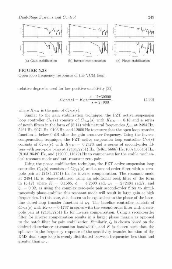
Dual-Stage Systems and Control 249
102 103 104−80
−60
−40
−20
0
20
Mag
nitu
de (d
B)
102 103 104−200
−100
0
100
200
Phas
e (d
eg)
Frequency (Hz)
(a) Gain stabilization
102 103 104−80
−60
−40
−20
0
20
Mag
nitu
de (d
B)
102 103 104−200
−100
0
100
200
Phas
e (d
eg)
Frequency (Hz)
(b) Inverse compensation
102 103 104−80
−60
−40
−20
0
20
Mag
nitu
de (d
B)
102 103 104−200
−100
0
100
200
Phas
e (d
eg)
Frequency (Hz)
(c) Phase stabilization
FIGURE 5.38Open loop frequency responses of the VCM loop.
relative degree is used for low positive sensitivity [33]
CCM (s) = KCMs+ 2π30000
s+ 2π900, (5.96)
where KCM is the gain of CCM (s).Similar to the gain stabilization technique, the PZT active suspension
loop controller CM (s) consists of CCM (s) with KCM = 0.18 and a seriesof notch filters in the form of (5.14) with natural frequencies fR,i at 2484 Hz,5461 Hz, 6074 Hz, 9103 Hz, and 12000 Hz to ensure that the open loop transferfunction is below 0 dB after the gain crossover frequency. Using the inversecompensation technique, the PZT active suspension loop controller CM (s)consists of CCM (s) with KCM = 0.2473 and a series of second-order fil-ters with zero-pole pairs at (2484, 2751) Hz, (5461, 5686) Hz, (6074, 6646) Hz,(9103, 9549) Hz, and (12000, 11672) Hz to compensate for the stable mechan-ical resonant mode and anti-resonant zero pairs.
Using the phase stabilization technique, the PZT active suspension loopcontroller CM (s) consists of CCM (s) and a second-order filter with a zero-pole pair at (2484, 2751) Hz for inverse compensation. The resonant modeat 2484 Hz is phase-stabilized using an additional peak filter of the formin (5.17) where K = 0.1585, φ = 4.2603 rad, ω1 = 2π2484 rad/s, andζ1 = 0.02, as using the complex zero-pole pair second-order filter to simul-taneously phase-stabilize this resonant mode will result in large gain at highfrequencies. In this case, φ is chosen to be equivalent to the phase of the base-line closed-loop transfer function at ω1. The baseline controller consists ofCCM (s) with KCM = 0.1737 in series with the second-order filter with a zero-pole pair at (2484, 2751) Hz for inverse compensation. Using a second-orderfilter for inverse compensation results in a larger phase margin as opposedto the notch filter for gain stabilization. Similarly, ζ1 is chosen based on thedesired disturbance attenuation bandwidth, and K is chosen such that thespillover in the frequency response of the sensitivity transfer function of theDMS dual-stage loop is evenly distributed between frequencies less than andgreater than ω1.

250 Advances in High-Performance Motion Control of Mechatronic Systems
A complex zero-pole pair second-order filter is also cascaded and insertedat (4600, 8000) Hz to provide phase lead which phase-stabilizes the resonantmodes at 5461 Hz and 6074 Hz. The damping ratios of the complex zeros andcomplex poles are 0.03 and 0.7, respectively. The zeros are lightly damped toprovide a sharp phase lead around 4600 Hz, and the poles are well damped toreduce the gain around 8000 Hz. Due to the presence of an input delay in thePZT active suspension, a partial inverse compensator is added to increase theamount of phase lead at 6074 Hz. In addition, a zero-pole pair is also cascadedand inserted at (6074, 6646) Hz for partial inverse compensation, and a first-order lag compensator with zero-pole pair at (15000, 6074) Hz is includedalong with notch filters in the form of (5.14) with natural frequencies fR,iat 9103 Hz and 13120 Hz. The first-order lag compensator is designed toreduce the high frequency gain amplification from the second-order filter withcomplex zero-pole pair at (4600, 8000) Hz and to phase-stabilize the resonantmode at 14240 Hz.
The mechanical resonant modes at frequencies ranging from 2484 Hz to12000 Hz are in-phase with the rigid-body mode, while the resonant modeat 14240 Hz is out-of-phase with the rigid-body mode. The resonant modesof the PZT active suspension at 2484 Hz, 5461 Hz, 6074 Hz, and 14240 Hzare phase-stabilized, and the resonant modes at 9103 Hz and 12000 Hz aregain-stabilized instead due to the amount of phase lag introduced by the inputdelay of the PZT active suspension. It is worth noting that the input delaymakes it possible for the out-of-phase resonant mode at 14240 Hz to be phase-stabilized.
The open loop frequency responses of the PZT active suspension loop,i.e., CM (s)PM (s), are shown in Figure 5.39.
102 103 104−80
−60
−40
−20
0
20
Mag
nitu
de (d
B)
102 103 104−200
−100
0
100
200
Phas
e (d
eg)
Frequency (Hz)
(a) Gain stabilization
102 103 104−80
−60
−40
−20
0
20
Mag
nitu
de (d
B)
102 103 104−200
−100
0
100
200
Phas
e (d
eg)
Frequency (Hz)
(b) Inverse compensation
102 103 104−60
−40
−20
0
20
Mag
nitu
de (d
B)
102 103 104−200
−100
0
100
200
Phas
e (d
eg)
Frequency (Hz)
(c) Phase stabilization
FIGURE 5.39Open loop frequency responses of PZT active suspension loop.
5.5.3 Simulation Results
In this section, simulation results of the above-mentioned dual-stage controldesign will be evaluated. For the combined dual-stage control, a DMS structureusing the gain stabilization, inverse compensation, and phase stabilization

Dual-Stage Systems and Control 251
resonance compensation methodologies will be used in the simulations. Thefrequency responses of open loop transfer functions LD using the DMS dual-stage control scheme are shown in Figure 5.40.
102 103 104−60
−40
−20
0
20
40
Mag
nitu
de (d
B)
102 103 104−200
−100
0
100
200
Phas
e (d
eg)
Frequency (Hz)
(a) Gain stabilization
102 103 104−60
−40
−20
0
20
40
Mag
nitu
de (d
B)
102 103 104−200
−100
0
100
200
Phas
e (d
eg)
Frequency (Hz)
(b) Inverse compensation
102 103 104−60
−40
−20
0
20
40
Mag
nitu
de (d
B)
102 103 104−200
−100
0
100
200
Phas
e (d
eg)
Frequency (Hz)
(c) Phase stabilization
FIGURE 5.40Frequency responses of open loop transfer functions using the DMS dual-stagecontrol scheme.
Using the gain-stabilization technique with notch filters in both theVCM and PZT active suspension loops, a dual-stage gain crossover fre-quency 1510 Hz is obtained, along with gain and phase margins of 14.1 dBand 31.8◦, respectively. Using the inverse compensation technique for boththe VCM and PZT active suspension loops, a dual-stage gain crossover fre-quency of 1520 Hz is obtained, along with gain and phase margins of 14.3 dBand 66.9◦, respectively. Using the phase-stabilization technique for both theVCM and PZT active suspension loops, a dual-stage gain crossover frequencyof 1640 Hz is obtained, along with gain and phase margins of 9.28 dBand 49.7◦, respectively. The second phase margin is 223.8◦.
The frequency responses of sensitivity transfer functions using the DMSdual-stage control scheme for the three different compensation methods areshown in Figure 5.41. It can be observed from these results that the VCM and
102 103 104−30
−25
−20
−15
−10
−5
0
5
10
Mag
nitu
de (d
B)
Frequency (Hz)
(a) Gain stabilization
102 103 104−30
−25
−20
−15
−10
−5
0
5
10
Mag
nitu
de (d
B)
Frequency (Hz)
(b) Inverse compensation
102 103 104−30
−25
−20
−15
−10
−5
0
5
10
Mag
nitu
de (d
B)
Frequency (Hz)
(c) Phase stabilization
FIGURE 5.41Frequency responses of sensitivity transfer functions using the DMS dual-stagecontrol scheme.
PZT active suspension do not compete with each other during actuation, and

252 Advances in High-Performance Motion Control of Mechatronic Systems
therefore they do not cause destructive interferences. At the hand-off frequencywhere the magnitudes of the VCM and PZT active suspension intersect, thephase difference between the VCM output and PZT active suspension outputis also much less than the suggested 120◦.
Table 5.4 shows the design specifications achieved using the above-mentioned controller designs.
TABLE 5.4Design Specifications Achieved with Dual-Stage Servo Controllers
Gain Inverse PhaseStabilization Compensation Stabilization
Order of CV 10 10 10Order of CM 11 11 14Hand-off frequency 304 Hz 371 Hz 317 HzPhase difference 84.9◦ 88.0◦ 86.7◦Gain crossover frequency 1.51 kHz 1.52 kHz 1.64 kHzGain margin 14.1 dB 14.3 dB 9.3 dBPhase margin 31.8◦ 66.9◦ 49.7◦||S||∞ 8.1 dB 2.7 dB 5.2 dB
5.6 Conclusion
In this chapter, various aspects of dual-stage systems and control from sys-tem identification (using continuous- and discrete-time measurements) todual-stage control topologies and controller design are detailed. In the ab-sence of extraneous sensors, the gain-stabilization, inverse compensation, andphase-stabilization techniques for resonance compensation are described. Thephase-stabilization design can be realized using the actuator’s in-phase me-chanical resonant modes, as well as additional add-on Linear Time-Invariant(LTI) or Linear Time-Varying (LTV) peak filters. With advanced sensor fu-sion, active damping of the mechanical resonant modes can be achieved viamulti-sensing or Self-Sensing Actuation (SSA) using direct-driven and indi-rect driven topologies on piezoelectric actuators. The additional displacementor strain information allows the mechanical resonant modes to be stiffened inthe inner loop by the developed model-based and non-model-based active con-trol methodologies. Using the HDD as a classic example of high-performancemechatronic systems, the effectiveness of the presented methodologies is eval-uated and verified on a commercial dual-stage 3.5" HDD with extensive sim-ulations and experiments.

Bibliography
[1] W. -I. Cho, N. -C. Park, H. Yang, and Y. -P. Park, “Swing-Arm-TypePZT Dual Actuator with Fast Seeking for Optical Disk Drive,” Microsys-tem Technologies, Vol. 8, Nos. 2–3, pp. 139–148, May 2002.
[2] K. H. Park, J. H. Lee, S. H. Kim, and Y. K. Kwak, “High Speed MicroPositioning System Based on Coarse/Fine Pair Control,” Mechatronics,Vol. 5, No. 6, pp. 645–663, September 1995.
[3] K. H. Park, C. H. Choi, and J. Ryu, “Hybrid Actuator for High Speedand High Precision Optical Disk Drives,” Mechatronics, Vol. 11, No. 5,pp. 527–543, August 2001.
[4] K. L. Hillsley and S. Yurkovich, “Vibration Control of a Two-Link Flexi-ble Robot Arm,” Dynamics and Control, Vol. 3, No. 3, pp. 261–280, July1993.
[5] A. Sharon, N. Hogan, and D. E. Hardt, “The Macro/Micro Manipulator:An Improved Architecture for Robot Control,” Robotics and Computer-Integrated Manufacturing, Vol. 10, No. 3, pp. 209–222, June 1993.
[6] D. Shin, I. Sardellitti, Y. L. Park, O. Khatib, and M. Cutkosky, “De-sign and Control of a Bio-Inspired Human-Friendly Robot,” InternationalJournal of Robotics Research, Vol. 29, No. 5, pp. 571–584, April 2010.
[7] B. S. Kim, J. Li, and T. C. Tsao, “Two Parameter Robust RepetitiveControl with Application to a Novel Dual-Stage Actuator for NoncircularMachining,” IEEE/ASME Transactions on Mechatronics, Vol. 9, No. 4,pp. 644–652, December 2004.
[8] A. T. Elfizy, G. M. Bone, and M. A. Elbestawi, “Design and Control ofa Dual-Stage Feed Drive,” International Journal of Machine Tools andManufacture, Vol. 45, No. 2, pp. 153–165, February 2005.
[9] C. W. Lee and S. W. Kim, “An Ultraprecision Stage for Alignment ofWafers in Advanced Microlithography,” Precision Engineering, Vol. 21.Nos. 2–3 pp. 113–122, September–December 1997.
[10] S. Woody and S. Smith, “Design and Performance of a Dual Drive Systemfor Tip-Tilt Angular Control of a 300 mm Diameter Mirror,” Mechatron-ics, Vol. 16 No. 7, pp. 389–397, September 2006.
253

254 Advances in High-Performance Motion Control of Mechatronic Systems
[11] S. K. Hung, E. T. Hwu, M. Y. Chen, and L. C. Fu, “Dual-Stage Piezoelec-tric Nano-Positioner Utilizing a Range-Extended Optical Fiber Fabry-Perot Interferometer,” IEEE/ASME Transactions on Mechatronics, Vol.12, No. 3, pp. 291–298, June 2007.
[12] D. S. Kang, T. Seo, Y. H. Yoon, B. S. Shin, X. -J. Liu, and J. Kim, “AMicro-Positioning Parallel Mechanism Platform with 100-Degree TiltingCapability,” CIRP Annals-Manufacturing Technology, Vol. 55, No. 1, pp.377–380, 2006.
[13] T. W. Seo, D. S. Kang, H. S. Kim, and J. Kim, “Dual Servo Controlof a High-Tilt 3-DOF Microparallel Positioning Platform,” IEEE/ASMETransactions on Mechatronics, Vol. 14, No. 5, pp. 616–625, October 2009.
[14] R. Evans, J. Griesbach, and W. Messner, “Piezoelectric Micro-Actuatorfor Dual-Stage Control,” IEEE Transactions on Magnetics, Vol. 35, No.2, pp. 977–982, March 1999.
[15] T. Hirano, L. Fan, W. Lee, J. Hong, W. Imaino, S. Pattanaik, S. Chan, P.Webb, R. Horowitz, S. Aggarwal, and D. Horsley, “High Bandwidth HighAccuracy Rotary Microactuator for Magnetic Hard Disk Drive TrackingServos,” IEEE/ASME Transactions on Mechatronics, Vol. 3, No. 3, pp.156–165, September 1998.
[16] H. Toshiyoshi, M, Mita, and T. Fujita, “A MEMS Piggyback Actuatorfor Hard Disk Drives,” IEEE Journal of Microelectromechanical Systems,Vol. 11, No. 6, pp. 648–654, December 2002.
[17] Y. Soeno, S. Ichikawa, T. Tsuna, Y. Sato, and I. Sato, “Piezoeletric Piggy-Back Microactuator for Hard Disk Drive,” IEEE Transactions on Mag-netics, Vol. 35, No. 2., pp. 983-987, March 1999.
[18] H. Fujita, K. Suzuki, M. Ataka, and S. Nakamura, “A Microactuator forHead Positioning System of Hard Disk Drives,” IEEE Transactions onMagnetics, Vol. 35, No. 2, pp. 1006–1010, March 1999.
[19] S. Koganezawa, K. Takashi, Y. Uematsu, T. Yamada, S. Hasegawa, andT. Ueno, “A Flexural Piggyback Milli-Actuator for Over 5 GBit/in2 Den-sity Magnetic Recording,” IEEE Transactions on Magnetics, Vol. 32, No.5, pp. 3908–3910, September 1996.
[20] J. Liu, K. Ono, J. Xu, J. Li, and M. Furukawa, “Thermal Actuator for Ac-curate Positioning Read/Write Element in Hard Disk Drive,” Microsys-tem Technologies, Vol. 18, Nos. 9–10, pp. 1583–1589, September 2012.
[21] L. Ljung, System Identification: Theory for the User, 2nd Edition, Pren-tice Hall, Englewood Cliffs, NJ, USA, 1999.

Bibliography 255
[22] T. Yamaguchi, M. Hirata, and C. K. Pang (eds.), High-Speed PrecisionMotion Control, CRC Press, Taylor and Francis Group, Boca Raton, FL,USA, 2011.
[23] M. Kawafuku, J. Eom, M. Iwasaki, and Hiromu Hirai “IdentificationMethod for Plant Dynamics Over Nyquist Frequency,” in Proceedingsof the 33rd Annual Conference of the IEEE IECON, pp. 362–367, Taipei,Taiwan, November 5–8, 2007.
[24] R. Ehrlich, C. Taussig, and D. Abramovitvh, “Identification of SampledData Systems at Frequencies Beyond the Nyquist Rate,” in Proceedingsof the IEEE CDC, pp. 646–652, Tampa, FL, USA, December 1989.
[25] M. Nagashima and S. Nakagawa, “Identification of the Secondary Ac-tuator Dynamics at Frequencies Beyond the Nyquist Rate in Dual-StageActuator Hard Disk Drive Systems,” Transactions of the Institute of Mea-surement and Control, Vol. 32, No. 2, pp. 188–210, April 2010.
[26] G. F. Franklin, J. D. Powell, and M. Workman, Digital Control of Dy-namic Systems, Addison-Weasley, 3rd Edition, 1997.
[27] C. Mohtadi, “Bode’s Integral Theorem For Discrete-Time Systems,” IEEProceedings D Control Theory and Applications, Vol. 137, No. 2, pp. 57–66, March 1990.
[28] R. Horowitz, Y. Li, K. Oldham, S. Kon, and X. Huang, “Dual-Stage ServoSystems and Vibration Compensation in Computer Hard Disk Drives,”Control Engineering Practice, Vol. 15, No. 3, pp. 291–305, March 2007.
[29] D. Abramovitch and G. Franklin, “A Brief History of Disk Drive Con-trol,” IEEE Control Systems Magazine, Vol. 22, No. 3, pp. 28–42, June2002.
[30] H. Uchida and T. Semba, “A Study of the Residual Vibration Duringthe Seek-Settling Period for Hard Disk Drives,” in Digests of the 2000APMRC, pp. MP19-1–MP19-2, Tokyo, Japan, November 6–8, 2000.
[31] C. K. Pang, F. Hong, and X. Wang, “Integrated Servo-Mechanical Con-trol Systems Design Using Nyquist Plots for High-Performance Mecha-tronics,” Microsystem Technologies, Vol. 18, Nos. 9–10, pp. 1719–1729,October 2012.
[32] C. K. Pang, S. C. Tam, G. Guo, B. M. Chen, F. L. Lewis, T. H. Lee,and C. Du, “Improved Disturbance Rejection with Online Adaptive Pole-Zero Compensation on a Φ-Shaped PZT Active Suspension,” Microsys-tem Technologies, Vol. 15, Nos. 10–11, pp. 1499–1508, October 2009.
[33] C. K. Pang, D. Wu, G. Guo, T. C. Chong, and Y. Wang, “Suppress-ing Sensitivity Hump in HDD Dual Stage Servo Systems,” MicrosystemTechnologies, Vol. 11, Nos. 8–10, pp. 653–662, August 2005.
256 Advances in High-Performance Motion Control of Mechatronic Systems
[34] M. Tomizuka, “Zero Phase Error Tracking Algorithm for Digital Con-trol,” Journal of Dynamic Systems, Measurement, and Control, Vol. 109,No. 1, pp. 65–68, March 1987.
[35] M. Kobayashi, S. Nakagawa, and S. Nakamura, “A Phase-Stabilized ServoController for Dual-Stage Actuators in Hard-Disk Drives,” IEEE Trans-actions on Magnetics, Vol. 39, No. 2, pp. 844–850, March 2003.
[36] L. Guo, “Reducing the Manufacturing Costs Associated with Hard DiskDrives—A New Disturbance Rejection Control Scheme,” IEEE/ASMETransactions on Mechatronics, Vol. 2, No. 2, pp. 77–85, June 1997.
[37] Y. -H. Kim, C. -I. Kang, and M. Tomizuka, “Adaptive and OptimalRejection of Non-Repeatable Disturbance in Hard Disk Drives,” in Pro-ceedings of the 2005 IEEE/ASME International Conference on AdvancedIntelligent Mechatronics, pp. 1–6, Monterey, CA, USA, July 24–28, 2005.
[38] J. Zheng, G. Guo, Y. Wang, and W. E. Wong, “Optimal Narrow-BandDisturbance Filter For PZT-Actuated Head Positioning Control on aSpinstand,” IEEE Transactions on Magnetics, Vol. 42, No. 11, pp. 3745–3751, November 2006.
[39] L. Sievers and A. Flotow, “Comparison and Extensions of Control Meth-ods For Narrow-Band Disturbance Rejection,” IEEE Transactions onSignal Processing, Vol. 40, No. 10, pp. 2377–2391, October 1992.
[40] W. Messner andM. Bodson, “Design of Adaptive Feedforward ControllersUsing Internal Model Equivalence,” in Proceedings of the 1994 Ameri-can Control Conference, pp. 1619–1623, Baltimore, MD, USA, June 29—July 1, 1994.
[41] K. B. Scribner, L. A. Sievers, and A. H. von Flotow, “Active Narrow-BandVibration Isolation of Machinery Noise from Resonance Substructure,”Journal of Sound and Vibration, Vol. 167, No. 1, pp. 17–40, October 1993.
[42] F. Hong and C. Du, “Stable Peak Filtering Method to Reject High Fre-quency Disturbance in Hard Disk Drives,” Journal of Advanced Mechan-ical Design, Systems, and Manufacturing, Vol. 4, No. 1, pp. 119–129,February 2010.
[43] S. -C. Pei and C. -C. Tseng, “Elimination of AC Interference in Electro-cardiogram Using IIR Notch Filter With Transient Suppression,” IEEETransactions on Biomedical Engineering, Vol. 42, No. 11, pp. 1128–1132,November 1995.
[44] R. Agarwal, E. I. Plotkin, and M. N. S. Swamy, “LMS-Optimal NotchFilters With Improved Transient Performance,” in Proceedings of the 37th
Midwest Symposium on Circuits and Systems, pp. 1019–1022, Lafayette,LA, USA, August 3–5, 1994.
Bibliography 257
[45] P. Sadovsky and K. Bartusek, “Optimisation of the Transient Responseof a Digital Filter,” Radioengineering, Vol. 9, No. 2, pp. 14–17, June 2000.
[46] C. K. Thum, C. Du, B. M. Chen, E. H. Ong, and K. P. Tan, “Midfre-quency Runout Compensation in Hard Disk Drives via a Time-VaryingGroup Filtering Scheme,” IEEE Transactions on Magnetics, Vol. 44,No. 12, pp. 4769–4779, December 2008.
[47] J. Piskorowski, “Digital Q-Varying Notch IIR Filter With TransientSuppression,” IEEE Transactions on Instrumentation and Measurement,Vol. 59, No. 4, pp. 866–872, April 2010.
[48] F. Hong and C. K. Pang, “A Peak Filtering Method with Improved Tran-sient Response for Narrow-Band Disturbance Rejection in Hard DiskDrives,” International Journal of Systems Science, in press.
[49] M. Kobayashi, T. Yamaguchi, T. Yoshida, and H. Hirai, “Multi-SensingServo with Carriage-Acceleration Feedback for Magnetic Disk Drives,” inProceedings of the 1998 American Control Conference, Vol. 5, pp. 3038–3042, Philadelphia, PA, USA, June 24–26, 1998.
[50] F. Y. Huang, W. Imaino, F. Lee, and T. Semba, “Active Damping inHDD actuator,” IEEE Transactions on Magnetics, Vol. 37, No. 2, pp.847–849, March 2001.
[51] S. -H. Lee, C. C. Chung, and C. W. Lee, “Active High-Frequency Vi-bration Rejection in Hard Disk Drives,” IEEE/ASME Transactions onMechatronics, Vol. 11, No. 3, pp. 339–345, June 2006.
[52] Y. Li, R. Horowitz, and R. Evans, “Vibration Control of a PZT Actu-ated Suspension Dual-Stage Servo System Using a PZT Sensor,” IEEETransactions on Magnetics, Vol. 39, No. 2, pp. 932–937, March 2003.
[53] J. J. Dosch, D. J. Inman, and E. Garcia, “A Self-Sensing PiezoelectricActuator For Collocated Control, Journal of Intelligent Material Systemsand Structures, Vol. 3, No. 1, pp. 166–183, 1992.
[54] C. K. Pang, G. Guo, Ben M. Chen, and T. H. Lee, “Self-Sensing Actuationfor Nanopositioning and Active-Mode Damping in Dual-Stage HDDs,”IEEE/ASME Transactions on Mechatronics, Vol. 11, No. 3, pp. 328–338,June 2006.
[55] H. Yamada, M. Sasaki, and Y. Nam, “Control of a Micro-Actuator forHard Disk Drives Using Self-Sensing Actuator, International Journal ofApplied Electromagnetics and Mechanics, Vol. 25, No. 1, pp. 247–259,2007.
[56] M. I. Friswell and D. J. Inman, “The Relationship Between Positive Po-sition Feedback and Output Feedback Controllers,” Smart Materials andStructures, Vol. 8, pp. 285-291, June 1999.

258 Advances in High-Performance Motion Control of Mechatronic Systems
[57] F. Hong and C. K. Pang, “Robust Vibration Control at Critical Reso-nant Modes Using Indirect-Driven Self-Sensing Actuation in MechatronicSystems,” ISA Transactions, Vol. 51, No. 6, pp. 834–840, November 2012.
[58] N. Jalili, M. Dadfarnia, F. Hong, and S. S. Ge, “Adaptive Non Model-Based Piezoelectric Control of Flexible Beams with Translational Base,”in Proceedings of the 2002 American Control Conference, pp. 3802–3807,Anchorage, AK, USA, May 8–10, 2002.
[59] G. Guo, D. Wu, and T. C. Chong, “Modified Dual-Stage Controller forDealing With Secondary-Stage Actuator Saturation,” IEEE Transactionson Magnetics, Vol. 39, No. 6, pp. 3587–3592, November 2003.
[60] S. J. Schroeck, W. C. Messner, and R. J. McNab, “On CompensatorDesign for Linear Time Invariant Dual-Input Single-Output Systems,”IEEE/ASME Transactions on Mechatronics, Vol. 6, No. 1, pp. 50-57,March 2001.
[61] L. Guo, D. Martin, and D. Brunnett, “Dual-Stage Actuator Servo Controlfor High Density Disk Drives,” in Proceedings of the 1999 IEEE/ASMEInternational Conference on Advanced Intelligent Mechatronics, pp. 132–137, Atlanta, GA, USA, September 19–23, 1999.
[62] M. Karaman and W. C. Messner, “Robust Dual-Stage HDD Track FollowControl Systems Design for Hand Off Shaping,” in Digests of the 2002APMRC, pp. BA5-01–BA5-02, Singapore, August 27–29, 2002.
[63] W. C. Messner, M. D. Bedillion, L. Xia, and D. C. Karns, “Lead andLag Compensators with Complex Poles and Zeros: Design Formulas forModeling and Loop Shaping,” IEEE Control Systems Magazine, Vol. 27,No. 1, pp. 44–54, February 2007.
6
Concluding Remarks from Editors
T. Yamaguchi
Ricoh Company Ltd.
M. Hirata
Utsunomiya University
C. K. Pang
National University of Singapore
CONTENTS
6.1 Transferring Technologies to Other Industries (T. Yamaguchi) . 2606.1.1 What is High-Speed Precision Motion Control? . . . . . . . . 2606.1.2 Sensing and Closing the Loop: Shifting Resource Power
to a Right Field . . . . . . . . . . . . . . . . . . . . . . . . . . . . . . . . . . . . . . . . . . 2616.1.3 Control Structure: Generating New Design Parameters 2626.1.4 Modeling: Necessity of Precise Disturbance Modeling . . 2636.1.5 Summary . . . . . . . . . . . . . . . . . . . . . . . . . . . . . . . . . . . . . . . . . . . . . . . . 263
6.2 What Can We Do when the Positioning Accuracy Reaches aLimit? (M. Hirata) . . . . . . . . . . . . . . . . . . . . . . . . . . . . . . . . . . . . . . . . . . . . . . 2676.2.1 Motivation . . . . . . . . . . . . . . . . . . . . . . . . . . . . . . . . . . . . . . . . . . . . . . . 2676.2.2 Support Vector Machine . . . . . . . . . . . . . . . . . . . . . . . . . . . . . . . . . 2676.2.3 Application to the Head-Positioning Control Problem in
HDDs . . . . . . . . . . . . . . . . . . . . . . . . . . . . . . . . . . . . . . . . . . . . . . . . . . . . 2696.2.3.1 Approach . . . . . . . . . . . . . . . . . . . . . . . . . . . . . . . . . . . . . 2696.2.3.2 Plant Model . . . . . . . . . . . . . . . . . . . . . . . . . . . . . . . . . . 2696.2.3.3 Training the Discriminant Function . . . . . . . . . . 2706.2.3.4 Validation . . . . . . . . . . . . . . . . . . . . . . . . . . . . . . . . . . . . 270
6.2.4 Summary . . . . . . . . . . . . . . . . . . . . . . . . . . . . . . . . . . . . . . . . . . . . . . . . 2726.3 Control Constraints and Specifications (C. K. Pang) . . . . . . . . . . . 274
6.3.1 Constraints and Limitations . . . . . . . . . . . . . . . . . . . . . . . . . . . . . 2746.3.1.1 Anti-Resonant Zeros . . . . . . . . . . . . . . . . . . . . . . . . . . 2766.3.1.2 Resonant Poles . . . . . . . . . . . . . . . . . . . . . . . . . . . . . . . 2776.3.1.3 Sensitivity Transfer Function . . . . . . . . . . . . . . . . 2776.3.1.4 Limitations on Positioning Accuracy . . . . . . . . 278
6.3.2 Bode’s Integral Theorem . . . . . . . . . . . . . . . . . . . . . . . . . . . . . . . . 279
259
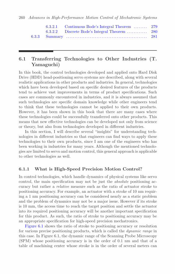
260 Advances in High-Performance Motion Control of Mechatronic Systems
6.3.2.1 Continuous Bode’s Integral Theorem . . . . . . . . 2796.3.2.2 Discrete Bode’s Integral Theorem . . . . . . . . . . . . 280
6.3.3 Summary . . . . . . . . . . . . . . . . . . . . . . . . . . . . . . . . . . . . . . . . . . . . . . . . 281
6.1 Transferring Technologies to Other Industries (T.Yamaguchi)
In this book, the control technologies developed and applied onto Hard DiskDrive (HDD) head-positioning servo systems are described, along with severalrealistic applications in other products and industries. In general, technologieswhich have been developed based on specific desired features of the productstend to achieve vast improvements in terms of product specifications. Suchcases are commonly encountered in industries, and it is always assumed thatsuch technologies are specific domain knowledge while other engineers tendto think that these technologies cannot be applied to their own products.However, it has been shown in this book that there are many cases wherethese technologies could be successfully transferred onto other products. Thismeans that new effective technologies can be developed not only from scienceor theory, but also from technologies developed in different industries.
In this section, I will describe several “insights” for understanding tech-nologies in different industries so that engineers can find ways to apply thesetechnologies to their own products, since I am one of the engineers who hasbeen working in industries for many years. Although the mentioned technolo-gies are limited to servo and motion control, this general approach is applicableto other technologies as well.
6.1.1 What is High-Speed Precision Motion Control?
In control technologies, which handle dynamics of physical systems like servocontrol, the main specification may not be just the absolute positioning ac-curacy but rather a relative measure such as the ratio of actuator stroke topositioning accuracy. For example, an actuator with a stroke of 10 nm requir-ing a 1 nm positioning accuracy can be considered nearly as a static problemand the problem of dynamics may not be a major issue. However if its strokeis 10 mm, the access time to reach the target position and settle the actuatorinto its required positioning accuracy will be another important specificationfor this product. As such, the ratio of stroke to positioning accuracy may bean appropriate specification for high-speed precision mechatronics.
Figure 6.1 shows the ratio of stroke to positioning accuracy or resolutionfor various precise positioning products, which is called the dynamic range inthis case. In Figure 6.1, the dynamic range of the Scanning Probe Microscopy(SPM) whose positioning accuracy is in the order of 0.1 nm and that of atable of machining center whose stroke is in the order of several meters can
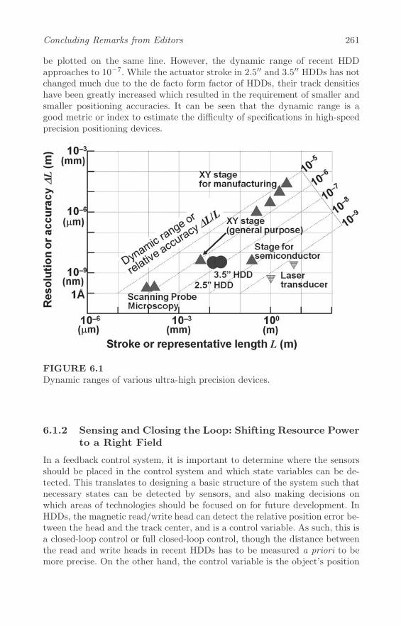
Concluding Remarks from Editors 261
be plotted on the same line. However, the dynamic range of recent HDDapproaches to 10−7. While the actuator stroke in 2.5′′ and 3.5′′ HDDs has notchanged much due to the de facto form factor of HDDs, their track densitieshave been greatly increased which resulted in the requirement of smaller andsmaller positioning accuracies. It can be seen that the dynamic range is agood metric or index to estimate the difficulty of specifications in high-speedprecision positioning devices.
FIGURE 6.1Dynamic ranges of various ultra-high precision devices.
6.1.2 Sensing and Closing the Loop: Shifting Resource Powerto a Right Field
In a feedback control system, it is important to determine where the sensorsshould be placed in the control system and which state variables can be de-tected. This translates to designing a basic structure of the system such thatnecessary states can be detected by sensors, and also making decisions onwhich areas of technologies should be focused on for future development. InHDDs, the magnetic read/write head can detect the relative position error be-tween the head and the track center, and is a control variable. As such, this isa closed-loop control or full closed-loop control, though the distance betweenthe read and write heads in recent HDDs has to be measured a priori to bemore precise. On the other hand, the control variable is the object’s position

262 Advances in High-Performance Motion Control of Mechatronic Systems
and the sensor can often detect the position of the actuator, e.g., a wafer onthe XY stage for semiconductor. In this case, the relative position error be-tween the object and the table may fluctuate due to temperature changes andcannot be detected, resulting in a semi closed-loop control.
During closed-loop control, the object is exactly on the right position whenits position error in a feedback loop is zero, but the plant dynamics and distur-bances are in the control loop. As such, the design of the feedback controllertends to be rather difficult in order to meet required performances while guar-anteeing robust stability. In the semi-closed loop control, the control of suchdynamics and disturbances is of utmost importance since some of the plantdynamics and disturbances are out of the feedback loop. Controlling the ambi-ent conditions such as temperature and active damping systems are commonlyused to stabilize or remove these effects since disturbances are the main issuein the design of the system.
When investigating the control systems of products in various industries, itcan be seen what technologies have been mainly developed for the products byrealizing how the control loop is closed. Sensor fusion and closing the controlloop are important issues at the basic structural design phase in the productdevelopment process.
6.1.3 Control Structure: Generating New Design Parame-ters
In the case of a simple control structure such as a single feedback loop us-ing a compensator like the Proportional-Integral-Derivative (PID) controller,the control design and its implementation are easier but the expected perfor-mance may be restricted due to less design parameters. On the other hand, acomplicated control structure may have more design parameters which mayimprove various performances, though it should be noted that complicatedimplementations may result in increased costs and longer execution time. Acomplicated control structure allows advanced control theories such as adap-tive control to be realized. Another possible advantage is to create new designparameters and find a way to improve targeted performances without deteri-orating or changing other performances. This is one of the greatest pleasuresof being an engineer in industries.
Examples of creating new design parameters by modifying the controlstructure are the Initial Value Compensation (IVC) using Mode SwitchingControl (MSC) as shown in Chapter 3, and a digital controller with variablemulti-rate sampling [1]. These examples are not just applications of advancedcontrol theories but rather modifying the control structure to create new de-sign parameters, and then improving the performances such as settling timeand acoustic noise.
After deciding on the basic structure of the control system, one of theimportant insights in designing a control structure is whether it is necessaryto add new design parameters to overcome any trade-offs of the control de-

Concluding Remarks from Editors 263
sign indices. In this case, additional components are required in the controlstructure to create such new design parameters.
6.1.4 Modeling: Necessity of Precise Disturbance Modeling
Recently, the importance of modeling has been well-recognized, such as themodel-based development approach, but modeling is mainly carried out on theplant or controlled object. In a typical feedback control system, the essenceof the control design is to design an optimal sensitivity transfer function fordisturbance and plant perturbation suppression, as well as an optimal comple-mentary sensitivity transfer function for robust stability. In other words, thecontrol design is a problem on how to find a compromise between them. How-ever, more sophisticated designs to improve positioning accuracy are requiredin HDD industries due to continuous requirements of storage capacity growth.As such, disturbance estimation and reduction using disturbance observersand learning or repetitive control to suppress specific periodic disturbanceshave been widely studied. Recently, precise loop-shaping based on detaileddisturbance modeling has also been studied.
A peak filter is designed to have high gain just at around 6.7 kHz where abig windage or disturbance caused by airflow is seen. The frequency responseof the controllers with and without windage compensation are shown in Fig-ure 6.2. The shaded region is the frequency range of windage, and the openloop characteristics of the system are shown in Figure 6.3. It can be seen thatthe proposed peak filter is phase-stable.
Since the peak filter reduces the amplitude of the sensitivity transfer func-tion at around 6.7 kHz very much as shown in Figure 6.4, the influence ofwindage is greatly reduced and the positioning accuracy is improved as shownby the PES spectra in Figure 6.5.
It is worth noting that 6.7 kHz is of much higher frequency as compared tothe bandwidth of feedback control. This implies that it is difficult to achievea high gain at such a high frequency range, but it is possible to find a way ofimproving positioning accuracy by modifying the controller accordingly oncethe characteristics of disturbances and plant (i.e., phase characteristics in thiscase) are precisely known. After fixing the control structure, we can designindividual controllers based on not only plant modeling but also disturbancemodeling as well.
6.1.5 Summary
In all, it is worthy to understand excellent servo control and motion controldeveloped for various industries and to try to apply them to your products. Inorder to do so, it is necessary to understand the basic features of the controlsystem. In this section, several insights on how to understand the features ofthe high-speed precision servo control system are shown along with the controlsystem development phases, i.e.,
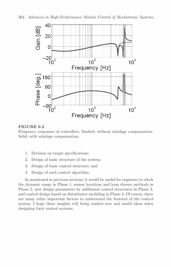
264 Advances in High-Performance Motion Control of Mechatronic Systems
FIGURE 6.2Frequency responses of controllers. Dashed: without windage compensation.Solid: with windage compensation.
1. Decision on target specifications;
2. Design of basic structure of the system;
3. Design of basic control structure; and
4. Design of each control algorithm.
As mentioned in previous sections, it would be useful for engineers to checkthe dynamic range in Phase 1, sensor locations and loop closure methods inPhase 2, new design parameters by additional control structures in Phase 3,and control design based on disturbance modeling in Phase 4. Of course, thereare many other important factors to understand the features of the controlsystem. I hope these insights will bring readers new and useful ideas whendesigning their control systems.

Concluding Remarks from Editors 265
(a) Bode diagram.
(b) Nyquist plot.
FIGURE 6.3Open loop characteristics of the system. Dashed: without windage compensa-tion. Solid: with windage compensation.

266 Advances in High-Performance Motion Control of Mechatronic Systems
FIGURE 6.4Frequency responses of sensitivity transfer functions of the system. Dashed:without windage compensation. Solid: with windage compensation.
FIGURE 6.5PES spectra. Dashed: without windage compensation. Solid: with windagecompensation.

Concluding Remarks from Editors 267
6.2 What Can We Do when the Positioning AccuracyReaches a Limit? (M. Hirata)
6.2.1 Motivation
To improve the positioning accuracies, much effort has been devoted to apply-ing various control theories in high-performance mechatronic systems. How-ever, what can we do when further improvements of the control accuracies areimpossible?
In many positioning control systems, the completion of the positioningphase must be determined correctly in order to initiate the start of the nexttask. For example in HDDs, the data read or write process cannot be starteduntil the R/W head (arriving from adjacent tracks) is settled at the center ofthe target track with an allowable positioning-error bound. As such, a fast andaccurate method of determining the completion of the positioning phase couldenhance the control performances further even when improvements in controlaccuracies are impossible. In particular, the determination will be difficultas the required control accuracy is higher than that of the current controlaccuracy and the output may exceed the tracking error bound again.
A simple way of determining the end of the positioning phase is to wait forseveral sampling periods in order to confirm that the output does not exceedthe error bound. This makes the unnecessary wait inevitable.
In this section, a method using Support Vector Machines (SVMs) is in-troduced [3]. The SVM is a well-known approach for classification, and usesa discriminant function to separate the data space into two regions. As such,the SVM has the ability to determine if the positioning phase has been fullycompleted.
6.2.2 Support Vector Machine
For given training data points (xi, yi) comprising of input data xi ∈ Rn andclass label yi ∈ {−1, 1}, the SVM is formulated as a problem to find a lineardiscriminant function f that separates the data points xi into two classesas [4]
f(xi) = 〈w,xi〉+ b, (6.1)
where 〈·, ·〉 is an inner-product, w is a normal vector of the hyperplane, andb is a bias term. As shown in Figure 6.6, the SVM separates the data pointsusing the hyperplane such that the distance from the hyperplane to the nearestdata point is maximized. The data points nearest to the hyperplane are calledsupport vectors.
The problem that maximizes the margin between the hyperplane and the

268 Advances in High-Performance Motion Control of Mechatronic Systems
01
1
FIGURE 6.6Training data and hyperplane.
nearest data point can be formulated as a quadratic programming problem as
minw,b
J (w) = minw,b
1
2〈w,w〉, (6.2)
subjected to (〈w,xi〉+ b)yi ≥ 1, i = 1, · · · , N, (6.3)
where the maximum margin is γ = 1/‖w‖. This formulation is also referredto as a primal problem. A Lagrange function is given by
L(w, b,α) = 〈w,w〉 −N∑i=1
αi{(〈w,xi〉+ b)yi − 1}. (6.4)
The dual problem
maxα
Q(α) = maxα
⎛⎝
N∑i=1
αi − 1
2
N∑i,j=1
yiyjαiαj〈xi,xj〉⎞⎠ ,
subjected to
N∑i=1
yiαi = 0, αi ≥ 0, i = 1, · · · , N, (6.5)
is obtained by differentiating (6.4) with respect to w, b and replacing themwith zeros.
When the data points are not linearly separable, they are mapped onto ahigher dimensional space using a nonlinear function φ(·) to make them separa-ble as shown in Figure 6.7. This is equivalent to using a nonlinear discriminantfunction
f(xi) = 〈w,φ(xi)〉+ b (6.6)
instead of (6.1).In general, the dimension of φ(xi) tends to be very high and optimization
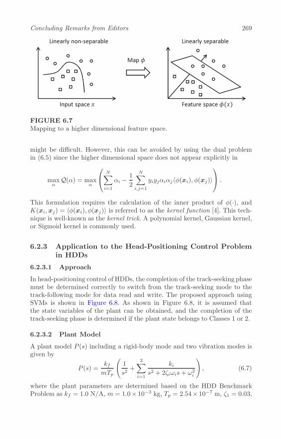
Concluding Remarks from Editors 269
Linearly non-separable Linearly separable
Input space � Feature space ����
Map �
FIGURE 6.7Mapping to a higher dimensional feature space.
might be difficult. However, this can be avoided by using the dual problemin (6.5) since the higher dimensional space does not appear explicitly in
maxα
Q(α) = maxα
⎛⎝
N∑i=1
αi − 1
2
N∑i,j=1
yiyjαiαj〈φ(xi), φ(xj)〉⎞⎠ .
This formulation requires the calculation of the inner product of φ(·), andK(xi,xj) = 〈φ(xi), φ(xj)〉 is referred to as the kernel function [4]. This tech-nique is well-known as the kernel trick. A polynomial kernel, Gaussian kernel,or Sigmoid kernel is commonly used.
6.2.3 Application to the Head-Positioning Control Problemin HDDs
6.2.3.1 Approach
In head-positioning control of HDDs, the completion of the track-seeking phasemust be determined correctly to switch from the track-seeking mode to thetrack-following mode for data read and write. The proposed approach usingSVMs is shown in Figure 6.8. As shown in Figure 6.8, it is assumed thatthe state variables of the plant can be obtained, and the completion of thetrack-seeking phase is determined if the plant state belongs to Classes 1 or 2.
6.2.3.2 Plant Model
A plant model P (s) including a rigid-body mode and two vibration modes isgiven by
P (s) =kfmTp
(1
s2+
2∑i=1
kis2 + 2ζiωis+ ω2
i
), (6.7)
where the plant parameters are determined based on the HDD BenchmarkProblem as kf = 1.0 N/A, m = 1.0× 10⁻³ kg, Tp = 2.54× 10⁻⁷ m, ζ1 = 0.03,

270 Advances in High-Performance Motion Control of Mechatronic Systems
FIGURE 6.8End of track-seeking phase determined using the SVM.
ζ2 = 0.01, ω1 = 2π4100 rad/s, ω2 = 2π7000 rad/s, k1 = −1.0, and k2 = −1.0.The state-space representation of (6.7) is omitted here due to limited space.It should be noted that the dimension of the state space is six.
6.2.3.3 Training the Discriminant Function
To extract training data from track-seeking responses, Final-State Control(FSC) inputs were obtained for a rigid-body mode model Pn = kf/(mTps
2).Pn was discretized using the Zero-Order Hold (ZOH) method at a samplingperiod of Ts = 37.879 μs, and the FSC inputs were obtained for variouscombination of seek distances from 10 to 900 tracks and seek times from 24to 130 sampling steps.
The obtained FSC inputs were applied to the plant having two vibrationmodes defined in (6.7), and the output responses were obtained. The magnifiedplot around the target track is shown in Figure 6.9 when the seek distance isfifty tracks. It should be noted that the initial positions were adjusted so thatthe target track is at Track 0. The allowable tracking-error bound is assumedto be ±0.03 of a track, which is shown by the dotted lines in Figure 6.9.
To construct a set of training data, the plant states where the correspond-ing outputs were located in the allowable tracking-error bound were collected.Next, the collected states were classified into two classes. Class 1 is a set of theplant states where the corresponding output exceeds the allowable tracking-error bound again after the current output, and Class 2 is a set of the plantstates where the corresponding output never exceeds the bound. Finally, thenonlinear discriminant function that separates Classes 1 and 2 was obtainedby the SVM using a 4th order polynomial kernel [4].
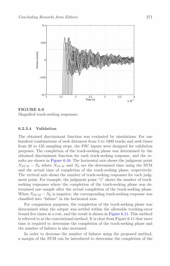
Concluding Remarks from Editors 271
1 1.5 2 2.5 3 3.5 4x 10⁻³
−0.1
−0.05
0
0.05
0.1
Time [s]
Posi
tion
[trac
k]
FIGURE 6.9Magnified track-seeking responses.
6.2.3.4 Validation
The obtained discriminant function was evaluated by simulations. For onehundred combinations of seek distances from 5 to 1000 tracks and seek timesfrom 20 to 135 sampling steps, the FSC inputs were designed for validationpurposes. The completion of the track-seeking phase was determined by theobtained discriminant function for each track-seeking response, and the re-sults are shown in Figure 6.10. The horizontal axis shows the judgment pointNSVM − N0 where NSVM and N0 are the determined time using the SVMand the actual time of completion of the track-seeking phase, respectively.The vertical axis shows the number of track-seeking responses for each judg-ment point. For example, the judgment point “1” shows the number of track-seeking responses where the completion of the track-seeking phase was de-termined one sample after the actual completion of the track-seeking phase.When NSVM −N0 is negative, the corresponding track-seeking response wasclassified into “failure” in the horizontal axis.
For comparison purposes, the completion of the track-seeking phase wasdetermined when the output was settled within the allowable tracking-errorbound five times in a row, and the result is shown in Figure 6.11. This methodis referred to as the conventional method. It is clear from Figure 6.11 that moretime is required to determine the completion of the track-seeking phase andthe number of failures is also increased.
In order to decrease the number of failures using the proposed method,a margin of the SVM can be introduced to determine the completion of the

272 Advances in High-Performance Motion Control of Mechatronic Systems
track-seeking phase on the safe side. This can be done by using the discrimi-nant function 〈w,x〉+ b = −0.8 instead of 〈w,x〉+ b = 0 in Figure 6.6. Theresult is shown in Figure 6.12, and it is confirmed that the number of failuresis drastically reduced. However, more time might be required to determinethe completion of the track-seeking phase in some cases.
6.2.4 Summary
In this example, the discriminant function was obtained by learning from thedata via simulations, though the training data from experiments can also beused. In this case, the plant model is not required, and nonlinearity of theplant will be incorporated in the discriminant function automatically.
In order to enhance the control performances of mechatronic systems, var-ious approaches other than merely increasing the positioning speeds and ac-curacies are also important. For this purpose, powerful tools such as the SVMdeveloped in other fields of research may provide significant improvements. Ihope this stimulates potential readers to find new and innovative approachesdeveloped in other areas of research.

Concluding Remarks from Editors 273
Failure 0 1 2 3 4 5 6 70
20
40
60
80
100
Judgment point
Num
ber o
f res
pons
es
FIGURE 6.10Simulation results of the proposed method using SVM.
Failure 0 1 2 3 4 5 6 70
20
40
60
80
100
Judgment point
Num
ber o
f res
pons
es
FIGURE 6.11Simulation results of the conventional method.
Failure 0 1 2 3 4 5 6 70
20
40
60
80
100
Judgment point
Num
ber o
f res
pons
es
FIGURE 6.12Simulation results of the proposed method using SVM when a margin is con-sidered.

274 Advances in High-Performance Motion Control of Mechatronic Systems
6.3 Control Constraints and Specifications (C. K. Pang)
In this section, the constraints and specifications of future high-performancemechatronic systems are detailed from a control theory perspective.
6.3.1 Constraints and Limitations
The block diagram of a typical sampled-data mechatronic system is shown inFigure 6.13. In Figure 6.13, a sampler is used in the place of the ZOH H(s)for brevity but without loss of generality.
FIGURE 6.13Block diagram of a typical sampled-data mechatronic system.
In this section, sampled-data systems will be handled using an approxi-mated continuous time system as shown in Figure 6.14.
FIGURE 6.14Block diagram of a continuous control system.
For simplicity but without loss of generality, consider the plant P = NP
DP
to be of Single Input Single Output (SISO) in series with controller C =
Concluding Remarks from Editors 275
NC
DCin a negative feedback configuration. In Figure 6.14, the plant P is the
mechanical actuator to be precisely controlled, and the controller C is thecontroller to be designed and synthesized.NC andNP are the zero polynomialsof C and P , respectively, while DC and DP are the pole polynomials of Cand P , respectively.
The open loop transfer function L is given by L = CP . The true output ywith input disturbances di, output disturbances do, and noise n in the servoloop can be obtained by
y = SPdi + Sdo − Tn, (6.8)
where S and T are the sensitivity transfer function and complementary sen-sitivity transfer function, respectively, defined by
S =1
1 + L=
1
1 + NCNP
DCDP
=DCDP
DCDP +NCNP, (6.9)
T =L
1 + L=
NCNP
DCDP
1 + NCNP
DCDP
=NCNP
DCDP +NCNP. (6.10)
The above relationships hold in both continuous and discrete time.In the standard unity negative feedback configuration shown in Figure 6.14,
there exist control conflicts and unavoidable trade-offs between attenuatingdisturbances as well as filtering measurement error and noise. For good track-ing performance and rejection of disturbances at low frequencies, effectivecontrol loop-shaping techniques are essential to avoid large control signalswhich saturate the mechatronic system.
From (6.8), it can be seen that a small S is ideal for disturbance rejection,while a small T is good for robustness against measurement noise and highfrequency uncertainties. Due to the immediate definitions of S and T in (6.9)and (6.10), respectively, the following identity always holds
S + T ≡ 1, (6.11)
i.e., S and T cannot be small simultaneously and in particular, |S| and |T |cannot be less than one-half at the same time. Fortunately, this conflict canbe resolved by making one transfer function small at one frequency band andthe other small at another. This is possible as the power spectra of referencesand disturbances are usually concentrated at low frequencies, while the powerspectra of measurement errors and noises are concentrated at high frequencies.
Knowing that T = SL as well as design specifications on S and T , an intu-itive approach to find the stabilizing controller C is via closed-loop synthesis,

276 Advances in High-Performance Motion Control of Mechatronic Systems
i.e.,
C = P−1L
= P−1S−1T. (6.12)
A problem now obviously arises as one has to choose among the many possiblearbitrary combinations of S and T although their solution “shapes” are known.The properness and characteristics of plant P are ignored and the controller Cderived via such a method might be non-causal, or even unstable if P is non-minimum phase.
As such, a more common and easier solution is to use the open loop ap-proach with L = CP . A good rule of thumb is to use high gain over low fre-quencies and decrease the gain as rapidly as possible after the gain crossoverfrequency. Cascading a large number of Low Pass Filters (LPFs) is not ad-missible due to the amount of phase lag introduced. Using Bode’s StabilityCriterion, the typical magnitude shape of a compensated open loop transferfunction of a negative feedback control system should have [5]
• Low frequency band: A large gain � 0 dB and descending with a slopeof −20N dB/dec;
• Mid frequency or crossover frequency band: Pass through 0 dB with ≈−20 dB/dec for stability; and
• High frequency band: A low gain < 0 dB and descending with a slopeof −20N dB/dec;
where N ∈ Z+\{1}.
The following results are presented.
6.3.1.1 Anti-Resonant Zeros
The presence of anti-resonant zeros implies blocking of certain signal fre-quencies by mechanical plant P . From (6.10), it can be seen that the zeropolynomial of the open loop transfer function L is the same as that of theclosed-loop transfer function T , i.e., the locations of the zeros are unaffectedby feedback control. As such, it is obvious that these zeros will inhibit inputdisturbance di rejection capabilities (by plant P ) as well as noise rejectionand tracking capabilities (by T ) at the frequencies of the anti-resonant zerosas can be seen from (6.8). To address the effects of stable anti-resonant zerosin P and T , corresponding stable poles are placed by feedback controller C inthe series compensation topology [6, 7].
In the presence of non-minimum phase (unstable) zeros, an undershoot willbe observed in the time responses with prolonged settling time. In addition,the closed-loop bandwidth has to be lowered as the extra phase lag intro-duced by these zeros reduces the phase margin. The magnitude and overallpositive area under the sensitivity transfer function also increase significantly
Concluding Remarks from Editors 277
at frequencies beyond the open loop bandwidth as depicted in the DiscreteBode’s Integral Theorem [8, 9]. To handle the effects of unstable zeros in Pand T , the Generalized Kalman-Yakubovic-Popov (GKYP) Lemma for inte-grated servo-mechanical design of the mechanical plant P is used to ensurethat T is positive real within a finite frequency range [10], by consideringthat a discrete-time system (with an equal number of inputs and outputs) isminimum phase if it is positive real [11].
6.3.1.2 Resonant Poles
Feedback control effectively shifts the location of closed-loop poles which canbe arbitrarily placed by designing C, if the mechanical plant P is controllable.From (6.9), it can be seen that the zeros of S are essentially the union set ofpoles of C and P . In order to create gain notches in S for enhanced disturbancerejection and error correction, the gain of the resonant poles in P should notbe fully compensated by using the phase-stabilization technique, e.g. [1, 12],or created by C using add-on peak filters, e.g. [13].
If C is chosen to be of low-order and the frequencies of mechanical reso-nant modes in P are fixed, the disturbance attenuation capabilities can onlybe achieved at high frequencies by decreasing the damping ratios of the polesin C and P . Similarly, the GKYP Lemma for integrated servo-mechanicaldesign of the mechanical plant P is used to ensure the mechanical resonantmodes (poles) of P are shaped to be in-phase based on finite frequency con-straints imposed on S [10].
6.3.1.3 Sensitivity Transfer Function
The sensitivity transfer function S is the transfer function from output dis-turbances do to the true output y or reference r to measured error e. As such,many existing loop-shaping methods in current literature put much emphasison improvements on tracking performances at low frequencies and disturbancerejection. One commonly used graphical tool for loop-shaping and control sys-tem design evaluation is the Nyquist plot. Two typical Nyquist curves L1(jω)and L2(jω) are shown in Figure 6.15, and the relationships between the openloop transfer function L(jω) and sensitivity transfer function S(jω) using theNyquist diagram are discussed in the continuous domain for brevity but with-out loss of generality.
Since S(jω) = 11+L(jω) with 1 + L(jω) as the output return difference
equation, the locus of |S(jω)| = 1 can be plotted as a unit disc with cen-ter at the critical point (−1 + j0). Define this disc as the Sensitivity Disc(SD) [6, 14]. For some frequencies ω− and ω+, an L(jω−) outside the SDresults in |S(jω−)| < 1 while an L(jω+) inside SD yields |S(jω+)| > 1 since|S(jω)| is the reciprocal of the distance of L(jω) to (−1 + j0). An L(jω) in-tersecting the SD corresponds to unity gain or 0 dB on the Bode Diagramof |S(jω)|.

278 Advances in High-Performance Motion Control of Mechatronic Systems
−3 −2 −1 0 1 2 3 4 5−3
−2
−1
0
1
2
3
Imag
inar
y
Real
FIGURE 6.15Nyquist plots. Solid: Sensitivity Disc (SD) with |S(jω)| = 1. Dashed: L1(jω).Dashed-dot: L2(jω).
As such, it can be seen from Figure 6.15 that L2(jω) will not have apositive area (or hump) in the sensitivity transfer function S. On the otherhand, L1(jω) enters the SD when ω ≥ ω+ and approaches the origin with aphase angle less than −π
2 . It is interesting to note that feedback is actuallydecreasing the performance of the control system when ω ≥ ω+ and the humpis increased.
With these constraints and limitations in mind, the controller C is designedto ensure that [6]
1. L(jω) is far from and does intersect with SD. If this is not possible,make L(jω) avoid SD where the frequency spectra of the distur-bances are concentrated;
2. L(jω) approach the origin at −π2 ≤ ∠L(jω) ≤ π
2 as ω → ∞ so thatthe SD is avoided. If this is not possible, make |L(jω)| ≈ 0 at thesefrequencies; and
3. L(jω) do not encircle (−1 + j0) clockwise for stability.
These considerations are valid for discrete time systems below the Nyquistfrequency as well.
6.3.1.4 Limitations on Positioning Accuracy
Assume that the input disturbances and noise are converted to an overalldisturbance model D at the output with Gaussian white noise input. The

Concluding Remarks from Editors 279
variance of true output y can be given by [15]
var(y) =1
π
∫ ∞
0
|S(jω)D(jω)|2 dω. (6.13)
Assume that the open loop transfer function L = CP is strictly proper andthe gain of L satisfies the following inequality for bandwidth requirement [16]as
|L(jω)| ≤ δ
(Ω
ω
)k+1
, (6.14)
where δ > 0 and k ≥ 1 are pre-specified scalars and δ < 0.5 is usuallyselected [17]. It is obvious that the gain of L is smaller than δ for all ω > Ωwhere Ω is the closed-loop bandwidth, and the roll-off is at least −20N dB/decwhere N ∈ Z
+\{1}.Using the definition of S, the following inequality is obtained
1
1 + δ(Ωω
)k+1≤ |S(jω)| ≤ 1
1− δ(Ωω
)k+1. (6.15)
The variance of true output y is bounded by [16]
var(y) ≥ Ω
πeβ +
1
π
∫ ∞
Ω
|D(jω)|2[1 + δ
(Ωω
)ke]2 dω, (6.16)
where ke = k+1 when k is odd, ke = k when k is even, and β =∫
Ω0
ln |D(jω)|2 dωΩ .
From (6.16), it can be seen that the positioning accuracy given by var(y) isa decreasing function of Ω. This supports the notion of improving positioningaccuracy via increasing the open loop bandwidth or gain crossover frequency,and illustrates the importance of an accurate disturbance model as depictedin the previous section. The shape of the sensitivity transfer function S is alsoimportant in improving the disturbance rejection capabilities, and is boundedby the Bode’s Integral Theorem.
6.3.2 Bode’s Integral Theorem
The Bode’s Integral Theorem was initially used to study the limitations of lin-ear control systems with non-minimum phase zeros or unstable poles. In thissection, the Continuous and Discrete Bode’s Integral Theorems are discussedalong with their implications on servo control of high-performance mecha-tronic systems.
6.3.2.1 Continuous Bode’s Integral Theorem
Theorem 1 Continuous Bode’s Integral Theorem [9]A continuous SISO and minimum phase Linear Time-Invariant (LTI) sys-tem has a stable open loop transfer function L(jω). The sensitivity transfer

280 Advances in High-Performance Motion Control of Mechatronic Systems
function of the unity negative feedback system is S(jω) = 11+L(jω) . If the
closed-loop system is stable, then∫ ∞
0
ln |S(jω)| dω = −π2Ks, (6.17)
where Ks = lims→∞ sL(s).
Corollary 1 When the relative degree of the open loop transfer func-tion L(jω) is greater than or equal to two, both Ks and the total area un-der the sensitivity transfer function S is zero. For |S(jω)| < 1 over somefrequency, it is necessary that |S(jω)| > 1 over another frequency range,thereby causing a degradation of disturbance rejection capabilities at frequen-cies whereby |S(jω)| > 1. This phenomenon is termed as the “waterbed” effect,and the relative degree of the open loop transfer function L(jω) has to be onefor unity gain of the sensitivity transfer function |S(jω)| at high frequencies.
For discrete time systems, the Discrete Bode’s Integral Theorem is morestringent and their conclusions differ.
6.3.2.2 Discrete Bode’s Integral Theorem
Theorem 2 Discrete Bode’s Integral Theorem [8, 9]A discrete time SISO and minimum phase LTI system has a stable open looptransfer function L(ejφ). The sensitivity transfer function of the unity negativefeedback system is S(ejφ) = 1
1+L(ejφ) . If the closed-loop system is stable, then
∫ π
−πln |S(ejφ)| dφ = 2π(− ln |Kz + 1|), (6.18)
where Kz = limz→∞ L(z), φ = ωT , and T is the sampling rate.
It is worth noting that the transfer functions are periodic about Nyquistfrequency π
T .
Corollary 2 When L(ejφ) is strictly proper, the Discrete Bode’s Integral The-orem in (6.18) reduces to
∫ π
−πln |S(ejφ)| dφ = 0. (6.19)
This is the waterbed effect in discrete time domain.
When the waterbed effect occurs, the magnitude of the peak of the sen-sitivity transfer function ||S||∞ is bounded by Theorem 2. Now supposethat |S(ejφ)| ≤ α < 1 and φ ∈ [−φ1, φ1], φ1 < π. From [17], it is straightfor-ward to see that
||S||∞ ≥(1
α
) φ1π−φ1
, (6.20)

Concluding Remarks from Editors 281
i.e., when the average magnitude of the sensitivity transfer function at lowfrequencies is −40 dB and the sampling frequency is 25 kHz, it can be shownthat ||S||∞ ≥ 3.5 dB if the bandwidth of the sensitivity transfer function isset at 1 kHz. As such, lowering the gain of the sensitivity transfer function atlow frequencies would result in a larger ||S||∞ at high frequencies (before theNyquist frequency).
Corollary 3 When L(ejφ) is proper with Kz < −2 or Kz > 0, then theDiscrete Bode’s Integral Theorem in (6.18) becomes
∫ π
−πln |S(ejφ)| dφ < 0. (6.21)
This implies that some loop-shaping technique is possible and may notbe bounded by the waterbed effect. This property is exploited during inte-grated servo-mechanical design of the mechanical plant P using the GKYPLemma [10].
Corollary 4 When L(ejφ) is proper with −2 < Kz < 0, the Discrete Bode’sIntegral Theorem in (6.18) implies that
∫ π
−πln |S(ejφ)| dφ > 0, (6.22)
and feedback control is now degrading sensitivity and performance rather thanimproving it.
This conclusion is similar to that of non-minimum phase systems.As a result, the presence of non-minimum zeros in the mechanical plant P
and delay from the sampled-data system causes overall positive sensitivity inmechatronic systems. However, this problem can be alleviated with the de-velopment of in-phase mechanical actuators, e.g. [18], with possible reductionto Corollary 2. This restricts the overall positive sensitivity area to zero andwithin the limits of the waterbed effect.
6.3.3 Summary
In this section, the constraints and specifications of future high-performancemechatronic systems have been described from a control theory perspective.Using a systems design methodology [19], the mechatronic system designproblem can be handled using both theoretical and graphical approaches.Our future works include development of a comprehensive integrated servo-mechanical framework considering negative-imaginary [20] and distribution-ally robust [21] properties, with specific applications to flexure-based magneticlevitation motors.


Bibliography
[1] T. Yamaguchi, M. Hirata, and C. K. Pang (eds.), High-Speed PrecisionMotion Control, CRC Press, Taylor and Francis Group, Boca Raton, FL,USA, 2011.
[2] T. Atsumi, T. Arisaka, T. Shimizu, and H. Masuda, “Head-PositioningControl Using Resonant Modes in Hard Disk Drives,” IEEE/ASMETransactions on Mechatronics, Vol. 10, No. 4, pp. 378–384, August 2005.
[3] A. Yokozuka and M. Hirata, “Determination of the End of Track Seekingof Hard Disk Drives Using Support Vector Machine,” in Proceedings ofthe 2012 ASME-ISPS/JSME-IIP Joint International Conference on Mi-cromechatronics for Information and Precision Equipment, pp. 358–360,Santa Clara, CA, USA, June 18–20, 2012.
[4] N. Cristianini and J. Shawe-Taylor, An Introduction to Support VectorMachines, Cambridge University Press, Cambridge, UK, 2000.
[5] J. Freudenberg, R. Middleton, and A. Stefanopoulou, “A Survey of In-herent Design Limitations,” in Proceedings of the 2000 American ControlConference, pp. 2987–3001, Chicago, IL, USA, June 28–30, 2000.
[6] C. K. Pang, D. Wu, G. Guo, T. C. Chong, and Y. Wang, “Suppress-ing Sensitivity Hump in HDD Dual-Stage Servo Systems,” MicrosystemTechnologies, Vol. 11, Nos. 8–10, pp. 653–662, August 2005.
[7] C. K. Pang, S. C. Tam, G. Guo, B. M. Chen, F. L. Lewis, T. H. Lee, andC. Du, “Improved Disturbance Rejection with Online Adaptive Pole-ZeroCompensation on a Phi-Shaped PZT Active Suspension,” MicrosystemTechnologies, Vol. 15, Nos. 10–11, pp. 1499–1508, October 2009.
[8] C. Mohtadi, “Bode’s Integral Theorem for Discrete-Time Systems,” IEEProceedings, Vol. 137, No. 2, pp. 57–66, March 1999.
[9] B. Wu and E. Jonckheere, “A Simplified Approach to Bode’s Theoremfor Continuous-Time and Discrete-Time Systems,” IEEE Transactionson Automatic Control, Vol. 37, No. 11, pp. 1797-1802, November 1992.
[10] Y. Z. Tan, C. K. Pang, F. Hong, and T. H. Lee, “Integrated Servo-Mechanical Design of High-Performance Mechatronics Using GeneralizedKYP Lemma,” Microsystem Technologies, in press.
283

284 Advances in High-Performance Motion Control of Mechatronic Systems
[11] L. Hitz and B. D. O. Anderson “Discrete Positive-Real Functions andTheir Application to System Stability,” IEE Proceedings, Vol. 116, pp.153–155, January 1969.
[12] M. Kobayashi, S. Nakagawa, and S. Nakamura, “A Phase-Stabilized ServoController for Dual-Stage Actuators in Hard-Disk Drives,” IEEE Trans-actions on Magnetics, Vol. 39, No. 2, pp. 844–850, March 2003.
[13] D. Wu, G. Guo, and T. C. Chong, “Midfrequency Disturbance Suppres-sion via Micro-Actuator in Dual-Stage HDDs,” IEEE Transactions onMagnetics, Vol. 38, No. 5, pp. 2189–2191, September 2002.
[14] C. K. Pang, F. Hong, and X. Wang, “Integrated Servo-Mechanical Con-trol Systems Design Using Nyquist Plots for High-Performance Mecha-tronics,” Microsystem Technologies, Vol. 18, Nos. 9–10, pp. 1719–1729,October 2012.
[15] Z. Li, G. Guo, B. M. Chen, and T. H. Lee “Optimal Track-FollowingDesign for the Highest Tracks per Inch in Hard Disk Drives,” Journal ofInformation Storage and Processing Systems, Vol. 3, Nos. 1–2, pp. 27–41,April 2001.
[16] D. Davison, P. Kabama, and S. Meerkov, “Limitation of Disturbance Re-jection in Feedback Systems with Finite Bandwidth,” IEEE Transactionson Automatic Control, Vol. 44, No. 66, pp. 1132-1144, June 1999.
[17] M. Seron, J. Braaslavsky, and G. Goodwin, Fundamental Limitations inFiltering and Control, Springer, London, UK, 1997.
[18] T. Arisaka, T. Shimizu, T. Atsumi, H. Masuda, and T. Yamaguchi, “De-velopment on In-Phase Actuator Mechanism in Hard Disk Drives,” inProceedings of the 2004 Asia-Pacific Magnetic Recording Conference,Seoul, Korea, August 16–19, 2004.
[19] C. K. Pang, T. S. Ng, F. L. Lewis, and T. H. Lee, “Managing ComplexMechatronics R&D: A Systems Design Approach,” IEEE Transactions onSystems, Man, and Cybernetics Part A: Systems and Humans, Vol. 42,No. 1, pp. 57–67, January 2012.
[20] J. Xiong, I. R. Petersen, and A. Lanzon, “Finite Frequency NegativeImaginary Systems,” IEEE Transactions on Automatic Control, Vol. 57,No. 11, pp. 2917–2922, November 2012.
[21] J. Goh and M. Sim, “Distributionally Robust Optimization and ItsTractable Approximations,” Operations Research, Vol. 58, No. 4: Part 1,pp. 902–917, July/August 2010.

Index
AAcceleration Feedforward Control (AFC), 4Acoustic noise, reduction of (HDD), 97–100
design of switching conditions, 99initial state sets, 99model-following control system, 98, 104mode switching, 98seeking noise, 97vibration, 98
AFC, see Acceleration Feedforward ControlAliasing, 205, 206Angle condition, 219Anti-resonant zeros, 276–277
BBang-bang input, 24Bode’s integral theorem, 279–281
continuous Bode’s integral theorem, 279–280discrete Bode’s integral theorem, 280–281loop-shaping technique, 281summary, 281“waterbed” effect, 280
Bumpy switching, prevention of, 96
CCMS, see Coupled Master-SlaveConcluding remarks from editors, 259–281
control constraints and specifications, 274–281anti-resonant zeros, 276–277Bode’s integral theorem, 279–281constraints and limitations, 274–279continuous Bode’s integral theorem, 279–280discrete Bode’s integral theorem, 280–281Generalized Kalman-Yakubovich-Popov Lemma, 276limitations on positioning accuracy, 278–279loop-shaping technique, 281Low Pass Filters, 276
285

286 Advances in High-Performance Motion Control of Mechatronic Systems
resonant poles, 277sensitivity transfer function, 277–278summary, 281unity gain, 277“waterbed” effect, 280
positioning accuracy reaches a limit, 267–273application to head-positioning control problem in HDDs, 269–
272approach, 269conventional method, 271Gaussian kernel, 269kernel function, 269kernel trick, 269Lagrange function, 268motivation, 267plant model, 269–270primal problem, 268Sigmoid kernel, 269summary, 272Support Vector Machine, 267–269training the discriminant function, 270validation, 271–272ZOH, 270
transferring technologies to other industries, 260–266, 260–266control structure (generating new design parameters), 262–263dynamic range, 260high-speed precision motion control, 260–261Initial Value Compensation using Mode Switching Control, 202precise disturbance modeling, 263Proportional-Integral-Derivative controller, 262Scanning Probe Microscopy, 260semi closed-loop control, 262shifting resource power to right field, 261–262summary, 263
Coupled Master-Slave (CMS), 244Current-feedback amplifier, 6
DD/A converter, see Digital-to-Analog converterDDSSA, see Direct-Driven SSADecoupled Master-Slave (DMS), 244DFT, see Discrete Fourier TransformDigital-to-Analog (D/A) converter, 6, 204Digital Signal Processor (DSP), 6Direct-Driven SSA (DDSSA), 232–234

Index 287
Discrete Bode’s Integral Theorem, 246, 276, 281Discrete Fourier Transform (DFT), 162Discrete-time measurement (dual-stage systems), 203–210
aliasing, 205, 206Digital-to-Analog converter, 204Linear Time-Invariant property, 204Nyquist frequency, 203Position Error Signal, 203pulse transfer function, 206single continuous-time sinusoid, 204system identification, 207ZOH, 207
DISO control structure, see Dual-Input-Single-Output control structureDMS, see Decoupled Master-SlaveDSA, see Dynamic Signal AnalyzerDSP, see Digital Signal ProcessorDual-Input-Single-Output (DISO) control structure, 243Dual-stage systems and control, 199–258
dual-stage controller design, 242–252control structure, 243–246Coupled Master-Slave, 244–245Decoupled Master-Slave, 245–246design example, 246–250Dual-Input-Single-Output parallel control structure, 243error correction, 242“hand-off” frequency, 247HDD dual-stage servo control, 244inverse compensation, 249Near Perfect Modeling, 246parallel, 243–244phase stabilization technique, 249PQ method, 244primary actuator controller (VCM loop), 247–248secondary actuator controller (PZT active suspension loop), 248–
250simulation results, 250–252Single-Input-Single-Output control system, 244
Micro Electrical Mechanical Systems, 200Pb-Zr-Ti active suspension, 200resonance compensation with extraneous sensors, 230–242
active damping, 231AMD controller, 237applications, 232balanced bridge circuit, 233closed-loop equation, 236

288 Advances in High-Performance Motion Control of Mechatronic Systems
damping ratio, 235, 236Direct-Driven SSA, 232–234Electro-Motive Force, 231Indirect-Driven SSA, 234–235model-based design, 235–238non-model-based design, 238–242notch filters, 239PI controller, 241PolyVinylDeneFlouride, 231PZT elements, 231Self-Sensing Actuation, 231–235strain feedback loop, 240under-actuation, 238
resonance compensation without extraneous sensors, 213–230angle condition, 219damping ratio, 227experimental verifications, 227–230frequency-shift methods, 222, 223gain stabilization, 214inverse compensation, 214–215inverse Laplace transform operator, 226Low Pass Filters, 214LTI peak filters, 215, 216–224phase-shift methods, 222phase stabilization, 215–227pseudo open loop transfer function, 217quality factor, 225using LTV peak filters, 224–227using mechanical resonant modes, 215–216Zero Phase Error Tracking controller, 215
system identification of dual-stage actuators in HDDs, 201–212aliasing, 205, 206continuous-time measurement, 202–203, 210–211Digital-to-Analog converter, 204discrete-time measurement, 203–210, 212–213Dynamic Signal Analyzer, 202“E” block, 202Laser Doppler Vibrometer, 202Linear Time-Invariant property, 204Nyquist frequency, 203, 212Position Error Signal, 203primary actuator (VCM), 202–209pulse transfer function, 206secondary actuator (PZT active suspension), 210–213single continuous-time sinusoid, 204

Index 289
system identification, 207yoke, 202ZOH, 207
Voice Coil Motor, 200Dynamic Signal Analyzer (DSA), 202
E“E” block, 202Electro-Motive Force (EMF), 231EMF, see Electro-Motive ForceEnd effector, 70Error correction, 242
FFast Fourier Transform (FFT), 168FFSC input, see Frequency-shaped Final State Control inputFFT, see Fast Fourier TransformFinal-State Control (FSC), 4, 33–39
augmented system, state-space representation of, 35final-state control with constraints, 38–39Fourier transform, 35, 37Frequency-shaped Final State Control input, 37Lagrange multiplier, 33minimum jerk input design, 34–35problem formulation, 33–34Quadratic Programming problem, 38spectrum of the control input, 35total positioning time, 35vibration minimized input design, 35–37
Focus servo, 113Fourier transform, FSC, 35, 37Frequency-shaped Final State Control (FFSC) input, 37FSC theory, see Final-State Control
GGain stabilization, dual-stage systems, 214Galvano mirror (reference switching), 114–123
current controlled amplifier, 114design of IVC, 123experimental position error, 115, 122experimental results, 123feedback controller, 115Integral-Proportional-Derivative compensator, 115mathematical model, 115–122point-to-point positioning, 115
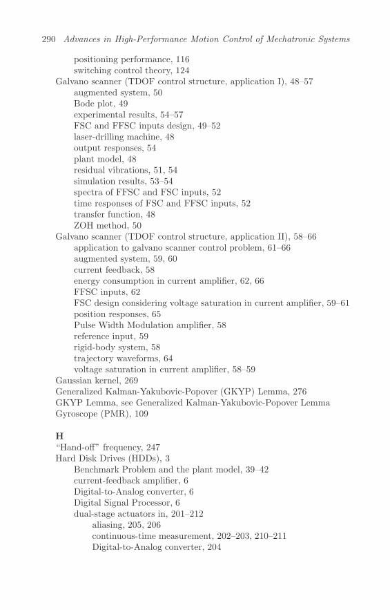
290 Advances in High-Performance Motion Control of Mechatronic Systems
positioning performance, 116switching control theory, 124
Galvano scanner (TDOF control structure, application I), 48–57augmented system, 50Bode plot, 49experimental results, 54–57FSC and FFSC inputs design, 49–52laser-drilling machine, 48output responses, 54plant model, 48residual vibrations, 51, 54simulation results, 53–54spectra of FFSC and FSC inputs, 52time responses of FSC and FFSC inputs, 52transfer function, 48ZOH method, 50
Galvano scanner (TDOF control structure, application II), 58–66application to galvano scanner control problem, 61–66augmented system, 59, 60current feedback, 58energy consumption in current amplifier, 62, 66FFSC inputs, 62FSC design considering voltage saturation in current amplifier, 59–61position responses, 65Pulse Width Modulation amplifier, 58reference input, 59rigid-body system, 58trajectory waveforms, 64voltage saturation in current amplifier, 58–59
Gaussian kernel, 269Generalized Kalman-Yakubovic-Popover (GKYP) Lemma, 276GKYP Lemma, see Generalized Kalman-Yakubovic-Popover LemmaGyroscope (PMR), 109
H“Hand-off” frequency, 247Hard Disk Drives (HDDs), 3
Benchmark Problem and the plant model, 39–42current-feedback amplifier, 6Digital-to-Analog converter, 6Digital Signal Processor, 6dual-stage actuators in, 201–212
aliasing, 205, 206continuous-time measurement, 202–203, 210–211Digital-to-Analog converter, 204
Index 291
discrete-time measurement, 203–210, 212–213Dynamic Signal Analyzer, 202“E” block, 202Laser Doppler Vibrometer, 202Linear Time-Invariant property, 204Nyquist frequency, 203, 212Position Error Signal, 203primary actuator (VCM), 202–209pulse transfer function, 206secondary actuator (PZT active suspension), 210–213single continuous-time sinusoid, 204system identification, 207yoke, 202ZOH, 207
dual-stage servo control, 244frequency response of nominal model, 7frequency response of perturbed plant model, 8head-positioning control system, 7, 136history and servo control, 8–12
application of control theories, 10–12growth in areal density, 8–10improvement of control structure, 12Linear Quadratic Gaussian/Loop Transfer Recovery, 11MEMS-based slider-driven actuators, 12Mode Switching Control structure, 11Non-Repeatable Run-Out, 9phase-stable control design, 11reference trajectory, design of, 10Repeatable Run-Out, 9technological development in servo control, 10–12
loop-sharing, 7magnetic head-positioning control in, 70mechanical structure, 5–6modeling, 6–8reduction of acoustic noise, 97–100
design of switching conditions, 99initial state sets, 99model-following control system, 98, 104mode switching, 98seeking noise, 97vibration, 98
schematic apparatus, 5spindle motor, 3Voice Coil Motor, 6
Hard Disk Drives (HDDs), positioning control, 175–195

292 Advances in High-Performance Motion Control of Mechatronic Systems
head-positioning control system, 175–177controlled object, 176delay-time element, 176repeatable runout, 176Voice Coil Motor, 175
residual vibrations, 188–195feedback control system, 189–190feedforward control system, 190–192simulation and experimental results, 192–195SRS analysis, 192ZOH, 189
sensitivity and complementary sensitivity transfer functions, 177–186design of control system, 178–180frequency responses, 179interpolation filter, 177magnitude response, 179multi-rate filter, 178simulation and experiment, 180–187time-domain simulations, 180validation of effects, 183
unobservable oscillations, 187–188dependence of sampling frequency, 187maximum displacement, 188
Hard Disk Drives (HDDs), TDOF control structure, 39–47FSC and FFSC inputs design, 42–47
design parameters, 45feedforward input, 43, 44output response, 43, 44track-seeking, 42
HDD Benchmark Problem and the plant model, 39–42Bode plots, 41parameter variations, 40track-seeking, 40
HDDs, see Hard Disk DrivesHigh-performance motion control of mechatronic systems, introduction to,
1–15brief history of HDD and its servo control, 8–12
application of control theories, 10–12growth in areal density, 8–10improvement of control structure, 12Linear Quadratic Gaussian/Loop Transfer Recovery, 11MEMS-based slider-driven actuators, 12Mode Switching Control structure, 11multi-sensing systems concept, 12Non-Repeatable Run-Out, 9

Index 293
phase-stable control design, 11reference trajectory, design of, 10Repeatable Run-Out, 9technological development in servo control, 10–12
concept, 1–5Acceleration Feedforward Control, 4Final-State Control theory, 4Hard Disk Drives, 3Initial Value Compensation, 4mechatronics, definition of, 1–2past studies, 45Proportional-Integral (PI) controller, 4Proximate Time Optimal Servomechanism, 4scope of book, 1–4settling controller, 3Shock Response Spectrum analysis, 4tracking error, 3Two-Degrees-of-Freedom control, 3Zero Phase Error Tracking Control, 4
hard disk drives as a classic example, 5–8current-feedback amplifier, 6Digital-to-Analog converter, 6Digital Signal Processor, 6frequency response of nominal model, 7frequency response of perturbed plant model, 8head-positioning control system, 7loop-sharing, 7mechanical structure, 5–6modeling, 6–8schematic apparatus, 5Voice Coil Motor, 6
IIDSSA, see Indirect-Driven SSAIEEJ, see Institute of Electrical Engineers of JapanIndirect-Driven SSA (IDSSA), 234–235Initial Value Compensation (IVC), 4Initial Value Compensation (IVC), transient control using, 69–133
background, 70–72end effector, 70free design parameters, 72linear robust control theory, 70Mode Switching Control, 71reference target, 71robot arm control, 70

294 Advances in High-Performance Motion Control of Mechatronic Systems
design of IVC, 78–97bumpy switching, prevention of, 96closed-loop poles, 88convolution matrix, 87cost function, 86design of additional input to controller, 84–89design of initial values on feedback controller, 79–83design of optimal switching condition, 89–97discrete-time domain, 92feedback controller, 84HDD head-positioning servo system, 81impulse response, 91jerk component, 87J-min-type IVC, 79Lagrange multiplier, 88Lyapunov equation, 92maximal output admissible set, 96mode switching, 80, 93performance indices, 92pole-zero-type IVC, 80positioning error, 96real coefficient matrix, 79reference trajectory, 90second-order lead-lag filter, 88track-seeking distance, 93transient responses, 82, 83undetermined real coefficients, 85vector signal, 95Voice Coil Motor, 94weighting coefficient for velocity, 82z-transformation, 86
industrial applications (mode switching), 97–114design of switching conditions, 99HDD (reduction of acoustic noise), 97–100initial state sets, 99model-following control system, 98, 104mode switching, 98optical disk drive, 113–114robot (Personal Mobility Robot), 100–113seeking noise, 97vibration, 98
industrial applications (reference switching), 114–123current controlled amplifier, 114design of IVC, 123experimental position error, 115, 122

Index 295
experimental results, 123feedback controller, 115galvano mirror for laser drilling machine, 114–123Integral-Proportional-Derivative compensator, 115mathematical model, 115–122point-to-point positioning, 115positioning performance, 116switching control theory, 124
Initial Value Compensation, 73–74coefficient matrix, 73HDD applications, 74TDOF controller, 73transfer function matrix, 73
optical disk drive, 113–114closed-loop system, 114focus servo, 113servo systems, 113state-space expression, 113tracking servo, 113
robot (Personal Mobility Robot), 100–113advantages, 100design of IVC, 111–112disadvantages, 100experimental results, 112–113feedback controller, initial value of, 109gear ratio, 110internal gyroscope, 109Lagrange equation of motion, 110mathematical model, 110–111stepwise torque reference, 109traveling mode, 100upper body, 110wheeled inverted pendulum mode, 110
switching control, overview of, 74–78closed-loop system, 76constrained control system, 76hybrid system, 74offline calculation method, 77strategy synthesis, 75supervisory role, 77target track, 78
Institute of Electrical Engineers of Japan (IEEJ), 39Integral-Proportional-Derivative (I-PD) compensator, 115Inverse Laplace transform operator, 226I-PD compensator, see Integral-Proportional-Derivative compensator

296 Advances in High-Performance Motion Control of Mechatronic Systems
IVC, see Initial Value Compensation
JJerk component, 87Jerk input, 24–26J-min-type IVC, 79
KKernel function, 269Kernel trick, 269
LLagrange equation of motion, 110Lagrange function, 268Lagrange multiplier, 33, 88Laser Doppler Vibrometer (LDV), 202LDV, see Laser Doppler VibrometerLinear Quadratic Gaussian (LQG), 11Linear Time-Invariant (LTI) property, 204Logic-based switching, 74Loop-sharing, 7Loop Transfer Recovery (LTR), 11Low Pass Filters (LPFs), 214, 276LPFs, see Low Pass FiltersLQG, see Linear Quadratic GaussianLTI property, 204LTR, see Loop Transfer RecoveryLyapunov equation, 92
MMATLAB script, example, 31Mechatronics
applications, 2definition of, 1–2
MEMS, see Micro Electrical Mechanical SystemsMicro Electrical Mechanical Systems (MEMS), 200MMTDOF control system, see Model-Matching Two-Degrees-Of-Freedom
control systemModel-Matching Two-Degrees-Of-Freedom (MMTDOF) control system,
20Mode switching (IVC), 97–114
design of switching conditions, 99HDD (reduction of acoustic noise), 97–100initial state sets, 99model-following control system, 98, 104
Index 297
mode switching, 98optical disk drive, 113–114robot (Personal Mobility Robot), 100–113seeking noise, 97vibration, 98
Mode Switching Control (MSC), 11, 71MSC, see Mode Switching ControlMulti-sensing systems concept, 12
NNear Perfect Modeling (NPM), 246Non-Repeatable Run-Out (NRRO), 9NPM, see Near Perfect ModelingNRRO, see Non-Repeatable Run-OutNyquist frequency
discrete-time measurement, 203dual-stage actuators in, Nyquist frequency, 203, 212residual vibrations, 164sampled-data systems, 148, 156SRS analysis, 164
OODOF control system, see One-Degree-Of-Freedom control systemOne-Degree-Of-Freedom (ODOF) control system, 18Optical disk drive, 113–114
closed-loop system, 114focus servo, 113servo systems, 113state-space expression, 113tracking servo, 113
PPb-Zr-Ti (PZT) active suspension, 200Personal Mobility Robot (PMR), 100–113
advantages, 100design of IVC, 111–112disadvantages, 100experimental results, 112–113feedback controller, initial value of, 109gear ratio, 110internal gyroscope, 109Lagrange equation of motion, 110mathematical model, 110–111stepwise torque reference, 109traveling mode, 100

298 Advances in High-Performance Motion Control of Mechatronic Systems
upper body, 110wheeled inverted pendulum mode, 110
PES, see Position Error SignalPI compensator, see Proportional-Integral compensatorPI controller, see Proportional-Integral controllerPID controller, see Proportional-Integral-Derivative controllerPMR, see Personal Mobility RobotPole-zero-type IVC, 80PolyVinylDeneFlouride (PVDF), 231Position Error Signal (PES), 203Positioning control, see Sampled-data systems, precise positioning control
inPQ method, 244Primal problem, 268Proportional-Integral (PI) compensator, 248Proportional-Integral (PI) controller, 4Proportional-Integral-Derivative (PID) controller, 262Proximate Time Optimal Servomechanism (PTOS), 4Pseudo open loop transfer function, 217PTOS, see Proximate Time Optimal ServomechanismPulse transfer function, 206Pulse Width Modulation (PWM) amplifier, 58PVDF, see PolyVinylDeneFlouridePWM amplifier, see Pulse Width Modulation amplifier
QQP problem, see Quadratic Programming problemQuadratic Programming (QP) problem, 38Quality factor, 225
RReference model, 20Reference switching (IVC), 114–123
current controlled amplifier, 114design of IVC, 123experimental position error, 115, 122experimental results, 123feedback controller, 115galvano mirror for laser drilling machine, 114–123Integral-Proportional-Derivative compensator, 115mathematical model, 115–122point-to-point positioning, 115positioning performance, 116switching control theory, 124
Relative acceleration model, 163
Index 299
Repeatable Run-Out (RRO), 9, 176Residual vibrations (sampled-data systems), 162–174
comparison between SRS and DFT, 168–170amplitude spectrum, 169Fast Fourier Transform, 168transient-state behavior, 170
Discrete Fourier Transform, 162residual vibration analysis based on SRS analysis, 162Shock Response Spectrum, 162SRS analysis, 162–163
output signal, 163relative acceleration model, 163shock response, 163steps, 163
SRS analysis using half-sine wave, 164–166Nyquist frequency, 164Zero-Order-Hold, 164, 165
SRS analysis using polynomial wave, 166–168damping ratio, 168discrete-time acceleration, 167
RMS amplitude, see Root-Mean-Square amplitudeRobot (Personal Mobility Robot), 100–113
advantages, 100design of IVC, 111–112disadvantages, 100experimental results, 112–113feedback controller, initial value of, 109gear ratio, 110internal gyroscope, 109Lagrange equation of motion, 110mathematical model, 110–111stepwise torque reference, 109traveling mode, 100upper body, 110wheeled inverted pendulum mode, 110
Root-Mean-Square (RMS) amplitude, 146RRO, see Repeatable Run-Out
SSampled-data polynomial input, 28–32Sampled-data systems, precise positioning control in, 135–198
calculation methods, 136–137continuous-time control system design, 136discrete-time control system design, 136hard disk drive example, 175–195

300 Advances in High-Performance Motion Control of Mechatronic Systems
controlled object, 176delay-time element, 176design of control system, 178–180feedback control system, 189–190feedforward control system, 190–192frequency responses, 179head-positioning control system, 175–177interpolation filter, 177magnitude response, 179multi-rate filter, 178repeatable runout, 176residual vibrations, 188–195sensitivity and complementary sensitivity transfer functions, 177–
186simulation and experiment, 180–187simulation and experimental results, 192–195SRS analysis, 192time-domain simulations, 180unobservable oscillations, 187–188dependence of sampling frequency, 187maximum displacement, 188
validation of effects, 183Voice Coil Motor, 175ZOH, 189
residual vibrations, 162–174amplitude spectrum, 169comparison between SRS and DFT, 168–170damping ratio, 168Discrete Fourier Transform, 162discrete-time acceleration, 167Fast Fourier Transform, 168Nyquist frequency, 164output signal, 163relative acceleration model, 163residual vibration analysis based on SRS analysis, 162shock response, 163Shock Response Spectrum, 162SRS analysis, 162–163SRS analysis using half-sine wave, 164–166SRS analysis using polynomial wave, 166–168steps, 163transient-state behavior, 170Zero-Order-Hold, 164, 165
sampled-data control system, 136

Index 301
sensitivity and complementary sensitivity transfer functions, 137–145,138–142
relationship between continuous- and discrete-time signals, 137–138
sampled-data control system using a multi-rate digital filter, 142–145
unobservable oscillations, 146–161definition of unobservable magnitude of oscillations, 146–147definition of unobservable magnitudes of oscillations with damp-
ing, 150–152example of unobservable magnitudes for oscillations with damp-
ing, 152–153histogram of event probability, 153, 155index of unobservable magnitudes, 154–161mechanical resonant frequency, 158Nyquist frequency, 156oscillations at Nyquist frequency, 148oscillations at one-third of sampling frequency, 150oscillations at sampling frequency, 147positioning control systems, 159relationship between oscillation frequency and unobservable mag-
nitude of oscillations, 146–150RMS value, 156Root-Mean-Square amplitude, 146unobservable magnitudes of oscillations with damping, 150–161worst-case unobservable magnitude, 147, 154write-inhibit condition, 151
Scanning Probe Microscopy (SPM), 260Self-Sensing Actuation (SSA), 231–235Shock response, 163Shock Response Spectrum (SRS), 4, 162Sigmoid kernel, 269Single-Input-Single-Output (SISO) system, 18, 244SISO systems, see Single-Input-Single-Output systemSPM, see Scanning Probe MicroscopySRS, see Shock Response SpectrumSSA, see Self-Sensing ActuationSupport Vector Machines (SVMs), 267SVMs, see Support Vector MachinesSwitching control (IVC), 74–78
closed-loop system, 76constrained control system, 76hybrid system, 74offline calculation method, 77strategy synthesis, 75

302 Advances in High-Performance Motion Control of Mechatronic Systems
supervisory role, 77target track, 78
Switching control theory, 124Symbolic Math Toolbox, 31
TTDOF (Two-Degrees-of-Freedom) control, 3TDOF control structure and optimal feedforward input, fast motion con-
trol using, 17–68final-state control, 33–39
augmented system, state-space representation of, 35final-state control with constraints, 38–39Fourier transform, 35, 37Frequency-shaped Final State Control input, 37Lagrange multiplier, 33minimum jerk input design, 34–35problem formulation, 33–34Quadratic Programming problem, 38spectrum of the control input, 35total positioning time, 35vibration minimized input design, 35–37
industrial application (galvano scanner I), 48–57augmented system, 50Bode plot, 49experimental results, 54–57FSC and FFSC inputs design, 49–52laser-drilling machine, 48output responses, 54plant model, 48residual vibrations, 51, 54simulation results, 53–54spectra of FFSC and FSC inputs, 52time responses of FSC and FFSC inputs, 52transfer function, 48ZOH method, 50
industrial application (galvano scanner II), 58–66application to galvano scanner control problem, 61–66augmented system, 59, 60current feedback, 58energy consumption in current amplifier, 62, 66FFSC inputs, 62FSC design considering voltage saturation in current amplifier,
59–61position responses, 65Pulse Width Modulation amplifier, 58
Index 303
reference input, 59rigid-body system, 58trajectory waveforms, 64voltage saturation in current amplifier, 58–59
industrial application (hard disk drives), 39–47Bode plots, 41design parameters, 45feedforward input, 43, 44FSC and FFSC inputs design, 42–47HDD Benchmark problem and the plant model, 39–42output response, 43, 44parameter variations, 40track-seeking, 40, 42
optimum feedforward input design, 23–32acceleration sampled-data polynomials, 32bang-bang input, 24boundary conditions, 25, 31digital implementation of minimum jerk input, 27–28MATLAB script, 31minimum jerk input, 24–26minimum time control, 23–24sampled-data polynomial input, 28–32Symbolic Math Toolbox, 31Zero-Order Hold, 27, 28
TDOF control structure, 18–23feedforward input, 22implementation of feedforward input, 22–23Model-Matching Two-Degrees-Of-Freedom control system, 20One-Degree-Of-Freedom control system, 18–19reference model, 20reference response property, 20Single-Input-Single-Output system, 18transfer matrix, 18two-degrees-of-freedom control system, 19–22
Tracking servo, 113Two-Degrees-of-Freedom control, see TDOF control
UUnder-actuation, 238Unity gain, 277Unobservable oscillations (sampled-data systems), 146–161, 187–188
dependence of sampling frequency, 187maximum displacement, 188relationship between oscillation frequency and unobservable magni-
tude of oscillations, 146–150

304 Advances in High-Performance Motion Control of Mechatronic Systems
definition of unobservable magnitude of oscillations, 146–147oscillations at Nyquist frequency, 148oscillations at one-third of sampling frequency, 150oscillations at sampling frequency, 147worst-case unobservable magnitude, 147
Root-Mean-Square amplitude, 146unobservable magnitudes of oscillations with damping, 150–161
definition, 150–152example of unobservable magnitudes for oscillations with damp-
ing, 152–153histogram of event probability, 153, 155index of unobservable magnitudes, 154–161mechanical resonant frequency, 158Nyquist frequency, 156positioning control systems, 159RMS value, 156worst-case unobservable magnitude, 154write-inhibit condition, 151
Upper body, 110
VVCM, see Voice Coil MotorVoice Coil Motor (VCM)
dual-stage systems, 200hard disk drive, 6, 175IVC design, 94
W“Waterbed” effect, 280Worst-case unobservable magnitude, 147, 154Write-inhibit condition, 151
YYoke, 202
ZZero-Order Hold (ZOH), 27, 28, 50
discrete-time measurement, 207dual-stage actuators, 207galvano scanner, 50position accuracy, 270residual vibrations, 189
Zero Phase Error Tracking Control (ZPETC), 4, 11Zero Phase Error Tracking (ZPET) controller, 215ZOH, see Zero-Order Hold

Index 305
ZPETC, see Zero Phase Error Tracking ControlZPET controller, see Zero Phase Error Tracking controllerz-transformation (IVC design), 86


![Model-based control for high-tech mechatronic systems · 6 Model-based control for high-tech mechatronic systems ongoing research on motion feedback control, including [63], [50],](https://img.dokumen.tips/doc/110x75/5ebad285f2dd182d6c4be394/model-based-control-for-high-tech-mechatronic-6-model-based-control-for-high-tech.jpg)