SYNTHESIS

Advances in Geometric Morphometrics

Philipp Mitteroecker Æ Philipp Gunz

Received: 4 February 2009 / Accepted: 5 February 2009

� The Author(s) 2009. This article is published with open access at Springerlink.com

Abstract Geometric morphometrics is the statistical

analysis of form based on Cartesian landmark coordinates.

After separating shape from overall size, position, and

orientation of the landmark configurations, the resulting

Procrustes shape coordinates can be used for statistical

analysis. Kendall shape space, the mathematical space

induced by the shape coordinates, is a metric space that can

be approximated locally by a Euclidean tangent space.

Thus, notions of distance (similarity) between shapes or of

the length and direction of developmental and evolutionary

trajectories can be meaningfully assessed in this space.

Results of statistical techniques that preserve these con-

venient properties—such as principal component analysis,

multivariate regression, or partial least squares analysis—

can be visualized as actual shapes or shape deformations.

The Procrustes distance between a shape and its relabeled

reflection is a measure of bilateral asymmetry. Shape space

can be extended to form space by augmenting the shape

coordinates with the natural logarithm of Centroid Size, a

measure of size in geometric morphometrics that is

uncorrelated with shape for small isotropic landmark

variation. The thin-plate spline interpolation function is the

standard tool to compute deformation grids and 3D visu-

alizations. It is also central to the estimation of missing

landmarks and to the semilandmark algorithm, which

permits to include outlines and surfaces in geometric

morphometric analysis. The powerful visualization tools of

geometric morphometrics and the typically large amount

of shape variables give rise to a specific exploratory style

of analysis, allowing the identification and quantification of

previously unknown shape features.

Keywords Asymmetry � Form space � Kendall shape

space � Procrustes � Semilandmarks � Thin-plate spline

Morphometrics, the measurement (metron) of shape

(morphe), is a subfield of statistics with a history going

back to the very beginnings of this discipline. For example,

in 1888 Frances Galton introduced the correlation coeffi-

cient and applied it to a variety of morphological

measurements on humans. In 1907 he invented a method to

quantify facial shape that has later been termed two-point

shape coordinates or Bookstein-shape coordinates (see

below). The application of multivariate statistical tech-

niques, which were basically developed in the first half of

the 20th century, led to so-called multivariate morpho-

metrics. But in the 1980s, morphometrics experienced a

major revolution through the invention of coordinate-based

methods, the discovery of the statistical theory of shape,

and the computational realization of deformation grids (for

historical reviews see Bookstein 1998; Rohlf and Marcus

1993; O’Higgins 2000; Adams et al. 2004; Slice 2005).

The ubiquitous application of fast personal computers has

ushered in a new era of data analysis, permitting the

exploration and visualization of large high-dimensional

P. Mitteroecker (&)

Konrad Lorenz Institute for Evolution and Cognition Research,

Adolf Lorenz Gasse 2, Altenberg A-3422, Austria

e-mail: philipp.mitteroecker@univie.ac.at

P. Mitteroecker

Department of Theoretical Biology, University of Vienna,

Althanstrasse 14, Vienna A-1091, Austria

P. Gunz

Department of Human Evolution, Max-Planck-Institute

for Evolutionary Anthropology, Deutscher Platz 6,

Leipzig D-04103, Germany

e-mail: gunz@eva.mpg.de

123

Evol Biol

DOI 10.1007/s11692-009-9055-x

data sets along with exact statistical tests based on

resampling procedures.

This new morphometric approach has been termed

geometric morphometrics as it preserves the geometry of

the landmark configurations throughout the analysis and

thus permits to represent statistical results as actual shapes

or forms. Among several geometric approaches to mor-

phometrics, the Procrustes method is the most widespread

and best understood in its mathematical and statistical

properties (Bookstein 1996; Small 1996; Dryden and

Mardia 1998). Other frequently used morphometric meth-

ods are Euclidian distance matrix analysis (Lele and

Richtsmeier 1991, 2001), elliptic Fourier analysis (Lestrel

1982), and non-label based approaches like voxel-based

morphometry (e.g., Ashburner and Friston 2000), which is

mainly applied in brain imaging. For more traditional

morphometric approaches see Blackith and Reyment

(1971), Marcus (1990), and Oxnard (1983), or the variety

of methods applied in histology (Baak and Oort 1983) and

stereology (Weibel 1979; Baddeley and Vedel Jensen

2004). For a rigorous statistical comparison of several of

these methods see Rohlf (2000a, 2000b, 2003). This article

focuses on Procrustes methods and the associated statistical

and graphical toolkit (Table 1 provides definitions of some

frequently used terms).

Geometric morphometrics is based on landmark coor-

dinates. Bookstein (1991, p. 2) defines landmarks as loci

that have names (‘bridge of the nose’, ‘tip of the chin’) as

well as Cartesian coordinates. The names are intended to

imply correspondence (biological homology) among

forms. That is, landmark points not only have their own

locations but also have the ‘‘same’’ locations in every other

form of the sample and in the average of all the forms.

These coordinate data can come from a vast array of

sources and can either be two- or three-dimensional. Two-

dimensional coordinates are usually captured using a dig-

itizing tablet or by measuring an image on the computer.

Three-dimensional data can be captured directly using a

coordinate digitizer such as a Microscribe or Polhemus, or

may be measured on surface scans or volumetric scans.

Volumetric data are based on image-slices from computed

tomographic (CT) or magnet resonance imaging (MRI)

scanners—or their high-resolution versions lCT and lMRI

(Sensen and Hallgrimsson 2009). These slices contain

gray-values that correspond to tissue densities and are

concatenated to obtain a three-dimensional representation

of an object. Surface scanners provide high-resolution 3D

representations of an object’s surface using either laser or

more traditional optical technology and may also include

texture information. Surfaces can also be extracted from

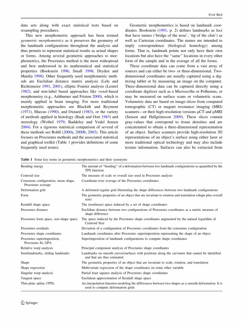
Table 1 Some key terms in geometric morphometrics and their synonyms

Bending energy The amount of ‘‘bending’’ of a deformation between two landmark configurations as quantified by the

TPS function

Centroid size The measure of scale or overall size used in Procrustes analysis

Consensus configuration, mean shape,

Procrustes average

Coordinate-wise average of the Procrustes coordinates

Deformation grid A deformed regular grid illustrating the shape differences between two landmark configurations

Form The geometric properties of an object that are invariant to rotation and translation (shape plus overall

size)

Kendall shape space The (nonlinear) space induced by a set of shape coordinates

Procrustes distance Euclidian distance between two configurations of Procrustes coordinates as a metric measure of

shape difference

Procrustes form space, size-shape space The space induced by the Procrustes shape coordinates augmented by the natural logarithm of

Centroid Size

Procrustes residuals Deviation of a configuration of Procrustes coordinates from the consensus configuration

Procrustes shape coordinates Landmark coordinates after Procrustes superimposition representing the shape of an object

Procrustes superimposition,

Procrustes fit, GPA

Superimposition of landmark configurations to compute shape coordinates

Relative warp analysis Principal component analysis of Procrustes shape coordinates

Semilandmarks, sliding landmarks Landmarks on smooth curves/surfaces with positions along the curvature that cannot be identified

and that are thus estimated

Shape The geometric properties of an object that are invariant to scale, rotation, and translation

Shape regression Multivariate regression of the shape coordinates on some other variable

Singular warp analysis Partial least squares analysis of Procrustes shape coordinates

Tangent space Euclidean approximation of Kendall shape space

Thin-plate spline (TPS) An interpolation function modeling the differences between two shapes as a smooth deformation. It is

used to compute deformation grids

Evol Biol

123

CT or MRI data. Most software packages allow landmark

coordinates to be measured directly on these virtual sur-

faces or volumetric objects.

Traditional (i.e., non-geometric) morphometric approa-

ches typically apply statistical techniques to a wide range

of measurements, such as distances and distance ratios,

angles, areas, and volumes. It is of course possible to

compute the traditional interlandmark distances and angles

from the landmark coordinates, but the original geometric

relationship among the points may not be reconstructable

from a sample of selected distance measurements. The raw

landmark coordinates, however, cannot be subject to sta-

tistical analysis before separating shape information from

overall size and ‘‘nuisance parameters’’ like position and

orientation of the specimens in the digitizing space that are

not relevant for the analysis.

The Geometry of Shape and Form

In morphometrics, the term shape is used to denote the

geometric properties of an object that are independent of

the object’s overall size, position, and orientation, whereas

the form of an object comprises both its shape and size.

Take, for example, the three landmarks A, B, and C in

Fig. 1, constituting a triangle as the simplest two-dimen-

sional configuration. The three interlandmark distances

sufficiently describe the triangle’s form: they are invariant

to rotation and translation, but contain information on

shape and overall scale. Another set of form variables

would be the distance between A and B, along with the two

perpendicular distances d and e. Angles are often avoided

in this context because of their demanding statistical

properties.

Shape variables, in contrast, are independent of the

overall size of a configuration and are often constructed by

dividing some interlandmark distances by a measure of

scale. In the absence of shape differences, overall size or

scale is an unambiguous concept and may be measured,

e.g., by any arbitrary interlandmark distance. When shape

varies across the observed geometries, size is less clearly

defined and requires either the (arbitrary) choice of a rep-

resentative single distance measure (usually one that is less

affected by the observed shape variation) or a quantity

based on a series of single size measures (such as Centroid

Size, see below, or the average of several distance mea-

surements). Another method to describe the shape of a

triangle is called two-point shape coordinates or Bookstein

shape coordinates (Bookstein 1991). Translate, scale, and

rotate the triangle in Fig. 1 until A has coordinates (0,0)

and B (1,0). The ensuing two coordinates of C (the shape

coordinates) sufficiently describe the shape of the triangle.

Alternatively, they can be computed as d and e divided by

the distance AB (the baseline size). A more general way to

compute shape coordinates, the Procrustes superimposi-

tion, is described below.

The shape of a triangle can be captured using two

variables only and thus has two degrees of freedom (df)

whereas the description of its form requires three df. In

addition to the information about the triangle’s shape, the

six coordinates of the three landmarks contain information

on scale (1 df), orientation (1 df), and position (2 df)—so

called nuisance parameters. In general, for p landmarks in k

dimensions, shape has pk-k-k(k-1)/2-1 df, that is four (for

two-dimensional data) or seven (3D) df less than the

number of landmark coordinates.

The two dimensions of shape for a triangle constitute a

two-dimensional shape space, in which a single point

represents the shape of a triangle. Interestingly, this shape

space is not a flat plane but has the form of the surface of a

sphere (Fig. 2); it is called Kendall shape space after the

Scottish mathematician who discovered it (Kendall 1981,

1984; Slice 2001). For more than three landmarks Kendall

shape space is a more complex Riemannian manifold

(a generalization to higher dimensions of a curved surface

in three dimensions). Kendall (1984) demonstrated that if

the vertices of a shape are independently and identically

distributed spherical normal variables, then the distribution

of shape is isotropic (the same in every direction) in

Kendall’s shape space (see also Bookstein 1991; Dryden

and Mardia 1998). This is an important property, guaran-

teeing that isotropic measurement error does not induce an

apparent ‘‘signal’’ in shape space.

An empirical analysis based on linear statistical

methods may thus be confounded by the non-linearity of

shape space, i.e., by variation in the pk shape coordinates

due to the curvature of shape space rather than due to

actual shape differences among the observed forms.

Because variation in biological shape is relatively small

even when observed across a wide range of different taxa,

it is possible to make a good linear approximation to the

non-linear shape space (Rohlf 1999; Marcus et al. 2000).

This linear space is of the same dimensionality as shapeFig. 1 Three landmarks A, B, and C constituting a triangle

Evol Biol

123

space and can be viewed as tangent to it, where the point

of tangency is at the reference shape (usually taken as the

sample average). Euclidean distances in this tangent

space closely resemble the distances in Kendall’s shape

space, so that the shapes projected into tangent space can

be used for analysis with standard multivariate methods.

Furthermore, the Euclidean geometry of tangent space

gives rise to meaningful notions of distance, length, and

direction, which are deeply entrenched in the rhetoric of

modern evolutionary and theoretical biology. For exam-

ple, distances (i.e., similarities) among individual shapes

or group mean shapes can be mutually related, and the

length and direction of developmental or evolutionary

trajectories can be meaningfully compared. This is not the

case for many classical ‘‘morphospaces’’ (Mitteroecker

and Huttegger, in press).

There are two principal ways to construct a tangent

space, but because of its geometric properties an orthog-

onal projection onto the space perpendicular to the vector

of shape coordinates of the reference shape is preferred in

most cases (see Rohlf 1999, for more details). Many

practitioners of morphometrics simply ignore the curva-

ture of shape space and apply standard multivariate

techniques to shape variables without prior projection into

tangent space. This may not be problematic for many data

sets (most linear methods, such as principal component

analysis, linearly approximate the curved shape space) but

may lead to serious artifacts when the variation within the

data is largely constrained to a single direction of shape

space (e.g., a single growth trajectory; see Mitteroecker

2007).

Procrustes Superimposition

For most practical applications, the parameters describing

the shapes for a sample of homologous landmark config-

urations are estimated by a Procrustes superimposition.

This procedure is a least-squares oriented approach

involving three steps (Fig. 3):

1. Translation of the landmark configurations of all

objects so that they share the same centroid (the

coordinate-wise average of the landmarks of one

form). Usually, this common centroid is sent to the

origin of the coordinate system.

2. Scaling of the landmark configurations so that they all

have the same Centroid Size—the square root of the

summed squared deviations of the coordinates from

their centroid. Centroid Size is a measure of scale for

landmark configurations, which has been shown to be

approximately uncorrelated with shape for small

isotropic landmark variation (Bookstein 1991; Dryden

and Mardia 1998). As a convention, Centroid Size is

set to one for all landmark configurations.

3. When superimposing two landmark configurations,

one of the two centered and scaled configurations is

rotated around its centroid until the sum of the squared

Euclidian distances between the homologous land-

marks is minimal. For more than two forms, this

algorithm has been extended to Generalized Procrustes

Analysis (GPA), where the rotation step is an iterative

algorithm (Gower 1975; Rohlf and Slice 1990). First,

all centered and scaled landmark configurations are

rotated to one arbitrary configuration of the sample

using the same least squares approach as above.

Subsequently, the resulting coordinates are averaged

and all configurations are rotated again to fit this

tentative consensus. These new coordinates are aver-

aged as an updated template for the next iteration. The

algorithm is repeated until convergence, which is

usually reached after a few iterations.

The coordinates of the resulting centered, scaled, and

rotated landmarks are called Procrustes shape coordinates;

their average (the consensus configuration) is the shape

whose sum of squared distances to the other shapes is

minimal and is thus the maximum likelihood estimate of

the mean for certain statistical models (Dryden and Mardia

1998). The individual differences from the average

shape are called Procrustes residuals. The Euclidian

(A) (B)Fig. 2 a The vertices of one

hundred random triangles

(independently and identically

distributed normal variables)

with an equilateral triangle as

the mean form. b The shapes of

these triangles are isotropically

distributed in Kendall’s shape

space, which has the form of the

surface of a (hemi)sphere

Evol Biol

123

distance between two sets of Procrustes shape coordinates

(i.e., the square root of summed squared coordinate-wise

differences) is referred to as Procrustes distance and

denotes the (dis)similarity in shape between two landmark

configurations.

Even though scaling the specimens to unit Centroid Size

resembles several other standard approaches to size cor-

rection, it is not the actual least squares solution. The

algorithm described above is therefore sometimes referred

to as partial Procrustes fitting. A smaller sum of squared

deviations among the landmark configurations can be

achieved by constraining the size of a configuration to the

cosine of the angle between the vector of shape coordinates

of that specimen and the vector of the mean shape. This

scaling approach results in the so-called full Procrustes fit

(Rohlf 1999). In most published analyses, however, only

partial Procrustes fitting is considered. Recently, Theobald

and Wuttke (2006) proposed a maximum-likelihood

approach to Procrustes superimposition (but see also

Bookstein 2007).

Due to the scaling step in the course of Procrustes

superimposition, the shape coordinates do not possess any

information on overall size—statistical results can only be

interpreted in terms of relative sizes within the observed

specimens. Yet, in many biological studies overall size is

an integral part of the assessed morphology and the anal-

ysis should be carried out in form space rather than in

shape space. In Mitteroecker et al. (2004a, 2005) we have

demonstrated that the Procrustes shape coordinates can be

augmented by the natural logarithm of Centroid Size to

construct Procrustes form space (also called size-shape

space). As for shape space, independently and identically

distributed spherical normal variation (such as measure-

ment error) around a mean form results in an isotropic

distribution in form space. Form space should be used

when both size and shape is of scientific concern, like in

classification studies or the analysis of development and

allometry. Developmental or evolutionary dissociation of

size and shape, such as in the context of heterochrony

(Zelditch 2001), can best be studied when contrasting

results in shape space and form space (Mitteroecker et al.

2004b, 2005; Gerber et al. 2007).

Deformation Grids

Visualization of shape differences and shape changes is a

primary aim and major strength of geometric morphomet-

rics. Morphological comparisons by deformations grids

date back to at least Albrecht Durer’s 1528 book ‘‘Vier

Bucher von menschlicher Proportion’’ and D’Arcy

Thompson’s (1915, 1917) pictorial approach of ‘‘Cartesian

transformations’’. Based on a mapping of homologous

point locations between forms, Thompson constructed

deformation grids illustrating how a part of one organism

may be described as a distortion of the same part in another

individual. Durer’s and Thompson’s approaches are visu-

ally appealing but their drawings were still made by hand

without any reference to a formal algorithm. It required fast

personal computers and the appropriate mathematics to

apply the idea of deformation grids on a computational

basis. After several other, meanwhile discarded attempts,

Bookstein (1989, 1991) introduced the method of thin-

plate spline (TPS) interpolation to compute deformation

grids in the style of Thompson and Durer. This algorithm,

borrowed from material physics, computes a mapping

function between two point configurations that maps the

measured points exactly while the space in-between is

smoothly interpolated. The notion of smoothness is

approached by minimizing the bending energy of the

deformation, a scalar quantity computed as the integral of

the squared second derivatives of that deformation. The

TPS formalism is also central to the semilandmark algo-

rithm and the estimation of missing data in morphometrics

(see below).

The TPS interpolation function from a template con-

figuration to a target configuration is usually applied to the

vertices of a regular grid so that the shape differences

between the two geometries can be read from the defor-

mation of this grid (Figs. 4 and 5a). When the actual shape

differences are subtle, the deformation can be extrapolated

by an arbitrary factor to ease the interpretation of the grid.

In the course of computation, the thin-plate spline function

is applied to each coordinate axis separately and can thus

be used for both two-dimensional and three-dimensional

data. Deformation grids have proved less effective for

Fig. 3 The three steps of

Procrustes superimposition:

translation to a common origin,

scaling to unit centroid size, and

rotation to minimize the sum of

squared Euclidean distances

among the homologous

landmarks. The resulting

landmark coordinates are called

Procrustes shape coordinates

Evol Biol

123

visualizing 3D shape differences, but because the mapping

function can be applied to any points in the vicinity of the

template landmarks, the algorithm can also be used to

deform a surface model (the vertices of a surface triangu-

lation) of the template specimen. A sequence of warped

surfaces can provide a useful alternative to deformation

grids for describing three-dimensional shape and form

differences (Fig. 5b).

The TPS function can also be applied to the pixels of an

image or to the voxels of volumetric data as derived from

CT or MRI scans. However, when warping the pixel

locations from the template to the target space according to

the two landmark configurations, pixels may overlap in the

target image (in areas of compression) or positions in the

image may be empty (in areas of expansion). To avoid such

fragmented images, the TPS algorithm is often used instead

to unwarp an image. The pixel positions of the target image

are warped to the template, identifying the pixels that

correspond across the two images. The gray values or the

color values of the target pixels are then substituted by the

corresponding values in the template image. The resulting

unwarped image is close (but not identical) to a respective

forward warping and is a continuous image with no gaps or

wholes (Fig. 5a).

In principle, bending energy is a measure of shape

difference between two landmark configurations, which

does not require Procrustes superimposition of the con-

figurations. It gives strong weight to shape differences at

a small geometric scale, while not taking into account

affine shape differences at all (shape deformations with

infinite scale). But bending energy is not a metric mea-

sure of distance (e.g., it is not symmetric) and hence is

usually not used for statistical analysis. The TPS for-

malism can also be applied to decompose shape

deformations into a range of geometrically independent

components (partial warps) with different geometric scale

and hence different bending energy (Bookstein 1989,

1991). A decomposition of the mean form (principal

warps) can be used as an orthogonal basis to span tangent

space, but is otherwise of limited biological relevance

(Rohlf 1998; Monteiro 2000).

Fig. 4 A template configuration (left) and a target configuration

(right) of five landmarks each. The deformation grid on the right

illustrates the thin-plate spline function between these configurations

as applied to the left regular grid—it is a visualization of the

differences between the two shapes

Fig. 5 a In a sample of 19 landmarks digitized on each of 691 cichlid

fish, the first principal component is visualized by a thin-plate spline

(TPS) function, applied to both a deformation grid and an image of a

fish. The left image represents a warp from the consensus configu-

ration (the average) to the negative direction of the principal

component whereas the right image is the opposite deformation, thus

representing a warp towards the positive direction (from Herler et al.,

in press). b Visualization of the average postnatal growth in the

hominoid cranium based on a shape regression on log Centroid size in

a sample of 96 landmarks and semilandmarks measured on 268

specimens. Starting from an average newborn, the TPS function is

applied at four equal steps along the vector of average growth to

the vertices of a surface triangulation, which was extracted from a

CT-scan (from Mitteroecker et al., 2004a). Note that while the TPS

function is applied directly to the deformation grid and the surface

triangulation (forward warping), the fish image is deformed by an

unwarping (see main text)

Evol Biol

123

Semilandmarks

All geometric morphometric tools strictly require that the

digitized landmarks are homologous across specimens, i.e.,

they represent the same biological locations in every indi-

vidual. Thus, anatomical landmarks need to be well defined

in all two or three dimensions of the digitizing space and

must be identifiable on all specimens in the sample. Typical

landmark locations are small cusps, invaginations, or

intersections of tissues such as bony sutures. In many

applications, however, point locations that fulfill all these

requirements are not evenly distributed across a biological

organism. A vertebrate skull, for example, has a large

number of anatomical landmarks in the face but only a few

points can be defined unambiguously on the smooth

braincase. Due to this limitation, most geometric morpho-

metric analyses of skull form have focused on the face and

the cranial base. The concept of semilandmarks (also called

sliding landmarks), first introduced in an appendix to the

‘‘Orange Book’’ (Bookstein 1991), was invented to extend

landmark-based statistics to smooth curves and surfaces. It

was first applied to two-dimensional outlines (Bookstein

1997) in a study of shape variability of sections of the

human corpus callosum (the structure that connects the left

and right hemispheres of our brain). In Gunz (2001, 2005)

and Gunz et al. (2005) we extended the algebra to curves

and surfaces in three dimensions. Alternative computational

approaches to semilandmarks can be found in Frost et al.

(2003) and Reddy et al. (2005).

Even though it is impossible to define an exact point-

to-point correspondence between landmarks on smooth

curves or surfaces, the semilandmark algorithm requires

that the structures themselves are homologous. While the

location of a landmark along the curvature may not be

identifiable, its coordinate perpendicular to the curvature is

well defined and driven by the observed morphology. The

semilandmark algorithm discards information derived from

the arbitrary spacing of semilandmarks along the curves or

surfaces, thus identifying the coordinates of biological

interest—the spacing of semilandmarks is produced as a

byproduct of the statistical analysis itself. This is achieved

by allowing the points to slide along their curve or surface

until some measure of shape difference among the con-

figurations is minimized. The two main semilandmark

algorithms differ in their optimization criteria: in one case

the bending energy of the thin-plate spline between each

specimen and the sample mean shape is minimized

whereas the Procrustes distances are minimized in the other

version of the algorithm.

To linearize the minimization problem, the semiland-

marks do not slide on the actual curve or surface but along

the tangent vectors to the curve or the tangent planes to the

surface (Fig. 6). Sliding of semilandmarks is an iterative

process repeating the following three steps: (1) computa-

tion of a tentative sample mean shape and of the tangent

vectors for each semilandmark in each specimen, (2)

sliding of semilandmarks along the tangents to minimize

either the Procrustes distances or the bending energy to the

mean, and (3) placing back the slid semilandmarks to the

nearest point on the curve or the surface, as they may slip

off the curvature (for relatively smooth curves this third

step may be omitted).

Fig. 6 When the location of a landmark on a smooth curve or surface

cannot be identified clearly, it may be treated as a semilandmark that

is allowed to slide along its curvature—only the position perpendic-

ular to the curve or surface carries a biological signal. As a

linearization of the underlying algorithm, the landmarks do not slide

along the actual curvature but on the tangent structures. For curves,

such as a section through a human corpus callosum in a or three-

dimensional ridge curves on a human cranium in b, the semiland-

marks are constrained to tangent vectors (the black and gray straight

lines, respectively). Semilandmarks on surfaces, such as the cranial

vault in b, are allowed to slide on tangent planes defined by two

vectors per semilandmark

Evol Biol

123

Semilandmarks have to be equal in number across the

sample and their starting positions should be in rough

geometrical correspondence. Clearly observable curves on

surfaces, such as ridges, should be treated as curves instead

of surface points. In general, the sampling of semiland-

marks depends on the complexity of curves or surfaces and

on the spatial scale of shape variation that is of interest.

Sampling experiments can help finding an ‘‘optimal’’

number of semilandmarks in the sense of how much

information additional points would contribute (Katina

et al. 2007).

To arrive at the same number of semilandmarks in the

same order on each specimen, it is convenient to begin with

points equidistantly spaced along outline arcs, e.g., through

automatic resampling of a polygonal approximation to the

curve. Techniques for surfaces differ substantially from

those for curves in that, except for planes and cylinders,

there is no straightforward analogue to the notion of ‘‘equal

spacing’’. We recommend beginning with a hugely

redundant sample of points on each surface, e.g., point

clouds generated by a surface scanner or extracted surfaces

from CT or MRI data. Alternatively, they can be produced

just by ‘‘scribbling’’ around the surface with a digitizing

device such as a Microscribe. On a single reference spec-

imen, one then produces a mesh of far fewer and relatively

evenly spaced points by thinning the redundant point cloud.

Points on this mesh should be denser near ridges of the

surface, especially if they are not treated as curves. This

reference mesh is then warped into the vicinity of the

surface of every other specimen using a thin-plate spline

interpolation function based on the anatomical landmarks

and the (yet unslid) curve-semilandmarks. On the surface

representation of each specimen the points nearest to the

warped mesh are taken as starting positions for the semi-

landmark algorithm. Through sliding the semilandmarks

acquire geometric homology or correspondence and can be

used in the subsequent statistical analyses just as if they

were classical landmarks.

Statistical Analysis

Statistical analysis in geometric morphometrics is per-

formed using the Procrustes shape coordinates (or other

representations of the organism’s geometry) and differs in

several respects from traditional approaches. In traditional

morphometrics, multivariate statistics is applied to a set of

measurements including distances, distance ratios, angles,

volumes, counts etc. As such variables often do not share

common units and comparable ranges of variation, they

typically are log transformed and standardized to unit

variance. Statistical analysis is thus usually based on cor-

relation matrices and comprises the full range of

multivariate techniques and statistical tests (see, e.g.,

Blackith and Reyment 1971; Marcus 1990; Oxnard 1983).

In geometric morphometrics the shape variables all possess

the same units so that analyses are based on the covariance

matrix and there exists a well-defined metric (the Pro-

crustes metric). Results of multivariate methods that

preserve this metric, such as principal component analysis,

multivariate regression, and partial least squares, can be

visualized as actual shapes or shape deformations in the

geometry of the original specimens. The algebra of the

statistical methods is the same for two- and three-dimen-

sional shape data; only the kind of visualization may differ

(see above).

Some methods which are popular in traditional mor-

phometrics, such as multiple regression, canonical

correlation analysis, and canonical variate analysis are not

equally useful in geometric morphometrics for several

reasons: most importantly they do not preserve the Pro-

crustes metric, discarding one of the core strengths of

geometric morphometrics. In addition, their computation

may be unreliable or impossible because these methods all

involve the inversion of the landmark variance-covariance

matrix. To compute a reliable matrix inverse, the number

of cases must exceed the number of variables, which is

often not the case in modern morphometrics. Also, Pro-

crustes shape coordinates usually are highly correlated

(especially when using semilandmarks), which results in a

singular covariance matrix that cannot be inverted. Even

when the number of variables is reduced, such as by

principal component analysis (see below), the results of

these methods may be difficult to interpret and to visualize

directly as shape deformations.

For example, canonical variate analysis (CVA), a pop-

ular method originally designed to classify unknown

individuals into pre-specified groups, is frequently used in

morphometrics in the style of an ordination technique and

to assess whether two or more groups differ in their mean

tendency. But when the number of variables is close to the

number of cases—a common situation in geometric mor-

phometrics—CVA will always separate groups even if they

actually possess the same mean. As a consequence, such

approaches are best avoided in geometric morphometrics

and a smaller range of multivariate methods has been

established as core statistical techniques.

Principal component analysis (PCA) is a method to

reduce a large set of variables to a few dimensions that

represent most of the variation in the data. PCA is com-

puted by an eigendecomposition of the sample covariance

matrix and is a rigid rotation of the data preserving the

Procrustes distances among the specimens. Principal

component scores are the projections of the shapes onto the

low-dimensional space spanned by the eigenvectors. They

can be plotted as two- or three-dimensional graphics and

Evol Biol

123

allow one to assess group differences, growth trends, out-

liers, etc., in the data without incorporating prior

information such as group affiliation; they are based on the

shape or form variables only. The eigenvectors or principal

components contain the weightings for the linear combi-

nations of the original variables and can be visualized as

actual shape deformations (relative warps, Bookstein 1991;

see also Fig. 5a). However, the principal components are

statistical artefacts largely depending on the composition of

the actual sample, and should not be interpreted as repre-

senting biologically meaningful factors (cf. Mitteroecker

et al. 2005; Mitteroecker and Bookstein 2007; Adams

et al., in review). There is one exception to this rule in

morphometrics: the first principal component of a single

species or population often represents allometry, the shape

variation induced by overall size variation (Klingenberg

1998). But this is only the case if allometric variation is the

dominant factor in the data, such as in an ontogenetic

sample, otherwise multivariate regression should be pre-

ferred to estimate allometry.

Multivariate regression of the shape variables on an

external variable (shape regression) is the method of

choice to assess the influence of a single factor such as a

functional or environmental variable, age, or the dose of a

drug on shape (Bookstein 1991; Monteiro 1999). The

regression of shape on the logarithm of Centroid Size is the

optimal measure of allometry (Mitteroecker et al. 2004a).

Multivariate regression is not sensitive to the number of

dependent shape variables or to their covariance structure

and the resulting vector of regression coefficients (quanti-

fying the average effect on shape) can be visualized as

shape deformation (Fig. 5b).

Partial least squares (PLS) is a method to assess rela-

tionships among two or more blocks of variables measured

on the same entities (Wold 1966; Rohlf and Corti 2000;

Bookstein et al. 2003). PLS yields linear combinations that

optimally (in a least-squares sense) describe the covari-

ances among the sets of variables and so provide a low-

dimensional basis to compare different blocks of variables.

Unlike canonical correlation analysis, the computation

does not involve the inversion of a matrix and the results

can be interpreted conveniently in terms of path models

and can be visualized as shape deformations (singular

warps). When all blocks of variables are comprised of

shape coordinates, PLS may be used to assess the ‘‘mor-

phological integration’’ among the respective anatomical

components (Bookstein et al. 2003; Bastir and Rosas 2006;

Gunz and Harvati 2007). As PLS only gives the patterns of

shape variation with the highest mutual covariance, but not

the corresponding amounts of these deformations (the

singular vectors are all scaled to unit length), a separate

scaling step may be necessary (Mitteroecker and Bookstein

2007, 2008). But the blocks may also be comprised of other

variables, such as functional, environmental, or behavioral

measures (e.g., Bookstein et al. 2002; Frost et al. 2003,

Manfreda et al. 2006), and PLS can be used to identify the

latent variables underlying the association among shape

and those factors.

Many geometric morphometric analyses are based on

randomization tests, such as permutation or bootstrap tests

(Manly 1991; Good 2000), rather than parametric methods

to assess the statistical significance level of a given

hypothesis. Most parametric tests require more cases than

variables and a specific (usually a normal) distribution of

the variables. Randomization tests, in contrast, are free

from these restrictions as long as the cases are sampled

independently. Furthermore, test statistics can be designed

even for complex hypotheses and compared with their

permutation distribution.

In summary, statistical analysis in geometric morpho-

metrics preserves the original geometry of the landmark

configurations and hence permits the visualization of

results as shape deformations. Together with the relatively

large amount of shape variables, this gives rise to a specific

exploratory style of analysis. Previously unknown shape

features can be inferred from visualizations such as TPS

deformation grids (e.g., Bookstein 2000) and vague notions

of a signal can be ‘‘calibrated’’ (Martens and Naes 1989)

with the present data. Instead of interpreting differences

along single shape coordinates or principal components, it

is more powerful to assess actual group mean differences,

shape regressions, and singular warps, which can be visu-

alized and directly related to the experimental design.

Traditional morphometrics, in contrast, is based on some

selected measures and the results are naturally restricted to

those few variables. Such classic multivariate analyses may

be sufficiently effective in assessing shape features known

prior to the data collection but are unlikely to produce

novel and unexpected findings.

Asymmetry

For bilateral objects, shape space can be partitioned into a

subspace of symmetric shape variation and a subspace of

asymmetric variation. The actual computation is based on a

Procrustes superimposition of the landmark configurations

together with their relabeled reflections (Bookstein 1991;

Klingenberg and McIntyre 1998; Mardia et al. 2000). The

Procrustes distance between a shape and its reflection is a

measure of asymmetry; it is zero only for perfectly sym-

metric shapes. A shape may be ‘‘symmetrized’’ by averaging

the shape and its superimposed reflection (Fig. 7). Con-

straining an analysis to the symmetric part of shape variation

reduces the degrees of freedom by discarding asymmetric

shape variation, including asymmetric measurement error,

which may not be of interest for the analysis.

Evol Biol

123

In a sample of shapes, asymmetric variation can be

decomposed further into directional asymmetry (the

asymmetry of the population mean) and fluctuating asym-

metry (asymmetric deviations from the population mean),

based on a multivariate analysis of variance. Fluctuating

asymmetry has been used to assess developmental insta-

bility (‘‘intra-individual variation’’) in many recent

investigations (e.g., Debat et al. 2000; Hallgrımsson et al.

2003; Schaefer et al. 2006; Willmore et al. 2006).

Missing Data in Morphometrics

From a statistical point of view, landmarks that cannot be

measured because anatomical structures are broken off or

deformed are termed ‘‘missing data’’. As geometric mor-

phometric methods require all measured specimens to have

the same number of landmarks at homologous positions,

the variables or the cases with missing values have to be

either excluded from the analysis, or the missing values

need to be estimated based on the available data. There

exists a large body of literature on methods for estimating

population parameters such as means or regressions in the

presence of missing values (for reviews and examples see

Schafer 1997; McLachlan and Krishnan 1997; Schafer and

Graham 2002). In morphometrics, particularly when

applied to the paleo-sciences, the estimates of the missing

values may be of interest themselves, e.g., as a way to

reconstruct fragmented fossils. In Gunz (2005) and Gunz

et al. (2004, in review) we have laid out a framework for

estimating missing shape coordinates, exploiting the high

redundancy of shape variables—especially when the mea-

surement points are closely spaced—and taking into

account prior biological knowledge about functional and

geometric constraints, symmetry, and morphological

integration.

The easiest yet most powerful way to deal with missing

and deformed anatomical structures is to restore bilateral

symmetry. When parts are missing on both sides or in the

symmetry plane, one can predict the coordinates of the

missing landmarks using information from complete cases.

Statistical reconstruction is aimed at optimizing the sta-

tistical likelihood of the estimate, using an extension of a

common missing data algorithm, the expectation-maximi-

zation method (Dempster et al. 1977), for Procrustes shape

variables. Geometric reconstruction employs the smooth-

ness properties of the thin-plate spline to estimate the

missing coordinates based on a single reference configu-

ration. A TPS interpolation is computed based on the

subset of landmarks that are available in both the reference

and the incomplete specimen. This interpolation function is

used to map the missing landmarks from the reference onto

the incomplete target, placing the landmark estimates so

that the deformation between the reference and the

incomplete specimen is as smooth as possible (minimum

bending energy). The reference configuration can be an

actual specimen or a Procrustes group average and may

resemble the incomplete specimens in properties such as

group affiliation, age, or geographic origin. Naturally,

choosing different references will result in slightly differ-

ent reconstructions. Whether similar conclusions may

follow from a variety of realistic alternative reconstructions

is testable in the course of the analysis: the distribution of

differently reconstructed shapes reflects the uncertainty due

to the missing data and the sensitivity to prior assumptions.

Morphometric Resources in the Internet

There emerged a range of free software for geometric

morphometric analysis in the last two decades. The Stony

Brook morphometrics site (life.bio.sunysb.edu/morph)

provides links for most of these software packages along

with morphometric data sets and bibliographies. The TPS

program series by James Rohlf, offering possibilities for

digitizing landmark, Procrustes superimposition including

semilandmarks, deformation grids, image warping, and

(A) (B)(D)

(C)

Fig. 7 Analysis of asymmetry in geometric morphometrics: a an

asymmetric configuration of 64 landmarks digitized on a photograph

of a human face. The configuration in b is the average of the

asymmetric shape a and its reflection c after Procrustes fitting,

resulting in a perfectly symmetric shape. The Procrustes distance

between a and c, which equals two times the distance between a and

b, is a measure of total asymmetry. The deformation grid d from the

symmetric consensus to the asymmetric shape in a visualizes the

pattern of asymmetry. This deformation is extrapolated by a factor of

three to ease its interpretation

Evol Biol

123

shape regression, became the standard tool for two-

dimensional landmark data. Several programs have been

developed to handle three-dimensional landmark data,

which mainly requires more extensive visualization tools.

The most comprehensive free software packages are

Morpheus et al. by Dennis Slice, Morphologika by Paul

O’Higgins, IMP by David Sheets, Past by Øyvind Ham-

mer, MorphoJ by Chris Klingenberg, and APS by Xavier

Penin. Morpheus et al., which offers elaborate 3D visual-

izations, and MorphoJ are written in Java and thus are

platform-independent. The Edgewarp3D package from Bill

Green and Fred Bookstein runs under Linux and Mac OS X

and provides tools for digitizing landmarks on 3D surfaces

and volumes, including semilandmarks on curves and

surfaces, together with many visualization options. With

the software package Landmark Editor (developed by UC

Davis in collaboration with the NYCEP morphometrics

group) one can measure landmarks on 3D surfaces and

capture semilandmarks by creating ‘‘patches’’ with equal

point count. Ian Dryden programmed several procedures

for statistical shape analysis in R (library ‘‘shapes’’) and

David Polly as well as Philipp Gunz and Philipp Mitter-

oecker developed a series of functions for geometric

morphometrics in Mathematica.

Further useful links can be found at www.morpho

metrics.org by Dennis Slice, including a possibility to

subscribe to the morphmet mailing list. An extensive

morphometrics glossary by Slice and co-workers is avail-

able at life.bio.sunysb.edu/morph/glossary/gloss1.html.

Acknowledgements We are grateful to Simon Huttegger, Astrid

Jutte, and Matthew Skinner for valuable comments on the manuscript

and thank Fred Bookstein, Dennis Slice, and Jim Rohlf for discussion.

Supported by grant GZ 200.033/1-VI/I/2004 of the Austrian Council

for Science and Technology, EU FP6 Marie Curie Research Training

Network MRTN-CT-2005-019564, and a fellowship from the Konrad

Lorenz Institute for Evolution and Cognition Research.

Open Access This article is distributed under the terms of the

Creative Commons Attribution Noncommercial License which per-

mits any noncommercial use, distribution, and reproduction in any

medium, provided the original author(s) and source are credited.

References

Adams, D. C., Rohlf, F. J., & Slice, D. E. (2004). Geometric

morphometrics: Ten years of progress following the ‘‘revolu-

tion’’. The Italian Journal of Zoology, 71(9), 5–16. doi:

10.1080/11250000409356545.

Adams, D. C., Cardini, A., Monteiro, L. R., O’Higgins, P., & Rohlf,

F. J. (in review). Morphometrics and Phylogenetics: principal

components of shape from cranial modules are neither appropriate

nor effective cladistic characters. Journal of Human Evolution.Ashburner, J., & Friston, K. J. (2000). Voxel-based morphometry—

The methods. NeuroImage, 11(6 I), 805–821.

Baak, J. P., & Oort, J. (1983). Morphometry in Diagnostic Pathology.

New York: Springer.

Baddeley, A. J., & Vedel Jensen, E. B. (2004). Stereology forStatisticians. Boca Raton: Chapman & Hall/CRC.

Bastir, M., & Rosas, A. (2006). Correlated variation between the

lateral basicranium and the face: A geometric morphometric

study in different human groups. Archives of Oral Biology,51(9), 814–824. doi:10.1016/j.archoralbio.2006.03.009.

Blackith, R. E., & Reyment, R. A. (1971). Multivariate morphomet-rics. London, New York: Academic Press.

Bookstein, F. L. (1989). Principal warps: Thin plate splines and the

decomposition of deformations. IEEE Transactions on PatternAnalysis and Machine Intelligence, 11, 567–585. doi:10.1109/

34.24792.

Bookstein, F. L. (1991). Morphometric tools for landmark data:geometry and biology (p. 435). New York: Cambridge Univer-

sity Press. xvii.

Bookstein, F. L. (1996). Biometrics, biomathematics and the

morphometric synthesis. Bulletin of Mathematical Biology,58(2), 313–365. doi:10.1007/BF02458311.

Bookstein, F. L. (1997). Landmark methods for forms without

landmarks: Morphometrics of group differences in outline shape.

Medical Image Analysis, 1(3), 225–243. doi:10.1016/S1361-

8415(97)85012-8.

Bookstein, F. L. (1998). A hundred years of morphometrics. ActaZoologica Academiae Scientarium Hungaricae, 44(1–2), 7–59.

Bookstein, F. (2000). Creases as local features of deformation grids.

Medical Image Analysis, 4(2), 93–110. doi:10.1016/S1361-8415

(00)00015-3.

Bookstein, F.L. (2007). Comment on ‘‘Maximum likelihood Procrustes

superpositions instead of least-squares’’. Posting at morphmet.

mailing list www.morphometric.org.

Bookstein, F. L., Gunz, P., Mitteroecker, P., Prossinger, H.,

Schaefer, K., & Seidler, H. (2003). Cranial integration in homo:

Singular warps analysis of the midsagittal plane in ontogeny and

evolution. Journal of Human Evolution, 44(2), 167–187. doi:

10.1016/S0047-2484(02)00201-4.

Bookstein, F. L., Streissguth, A. P., Sampson, P. D., Connor, P. D., &

Barr, H. M. (2002). Corpus callosum shape and neuropsycho-

logical deficits in adult males with heavy fetal alcohol exposure.

NeuroImage, 15(1), 233–251. doi:10.1006/nimg.2001.0977.

Debat, V., Alibert, P., David, P., Paradis, E., & Auffray, J. C. (2000).

Independence between canalisation and developmental stability

in the skull of the house mouse. Proceedings of the Royal Societyof London biology, 267(1442), 423–430.

Dempster, A., Laird, N., & Rubin, D. (1977). Maximum likelihood

from incomplete data via the EM algorithm. Journal of the RoyalStatistical Society. Series B, 39(1), 1–38.

Dryden, I. L., & Mardia, K. V. (1998). Statistical Shape Analysis.

New York: John Wiley and Sons.

Frost, S. R., Marcus, L. F., Bookstein, F. L., Reddy, D. P., & Delson,

E. (2003). Cranial allometry, phylogeography, and systematics

of large-bodied papionins (primates: Cercopithecinae) inferred

from geometric morphometric analysis of landmark data. TheAnatomical Record. Part A, Discoveries in Molecular, Cellularand Evolutionary Biology, 275(2), 1048–1072.

Gerber, S., Neige, P., & Eble, G. J. (2007). Combining ontogenetic and

evolutionary scales of morphological disparity: A study of early

Jurassic ammonites. Evolution & Development, 9(5), 472–482.

Good, P. (2000). Permutation tests: a practical guide to resamplingmethods for testing hypotheses. New York: Springer.

Gower, J. (1975). Generalized procrustes analysis. Psychometrika,40(1), 33–51. doi:10.1007/BF02291478.

Gunz, P. (2001). Using semilandmarks in three dimensions to model

human neurocranial shape (Master Thesis, University of Vienna,

Vienna, 2001).

Evol Biol

123

Gunz, P. (2005). Statistical and geometric reconstruction of hominid

crania: Reconstructing australopithecine ontogeny (Ph.D. Thesis,

University of Vienna, Vienna, 2005).

Gunz, P., & Harvati, K. (2007). The Neanderthal«chignon»: Varia-

tion, integration, and homology. Journal of Human Evolution,52(3), 262–274. doi:10.1016/j.jhevol.2006.08.010.

Gunz, P., Mitteroecker, P., & Bookstein, F. L. (2005). Semilandmarks

in three dimensions. In D. E. Slice (Ed.), Modern morphometricsin physical anthropology (pp. 73–98). New York: Kluwer

Academic/Plenum Publishers.

Gunz, P., Mitteroecker, P., Bookstein, F. L., & Weber, G. W. (2004).

Computer aided reconstruction of incomplete human crania

using statistical and geometrical estimation methods. Enter the

past: Computer applications and quantitative methods in archae-

ology. Oxford. BAR International Series, 1227, 96–98.

Gunz, P., Mitteroecker, P., Neubauer, S., Weber, G. W., & Bookstein,

F. L. (in review). Principles for the virtual reconstruction of

hominin crania. Journal of Human Evolution.

Hallgrımsson, B., Miyake, T., Wilmore, K., & Hall, B. K. (2003).

Embryological origins of developmental stability: Size, shape

and fluctuating asymmetry in prenatal random bred mice.

Journal of Anatomy, 208(3), 361–372.

Herler, J., Maderbacher, M., Mitteroecker, P., & Sturmbauer, C.

(in press). Sexual dimorphism in seven populations of Tropheus

(Teleostei: Cichlidae) from Lake Tanganyika.

Katina, S., Bookstein, F. L., Gunz, P., & Schaefer, K. (2007). Was it

worth digitizing all those curves? A worked example from

craniofacial primatology. American Journal of Physical Anthro-pology, S44, 140.

Kendall, D. (1981). The statistics of shape. In V. Barnett (Ed.),

Interpreting multivariate data (pp. 75–80). New York: Wiley.

Kendall, D. (1984). Shape manifolds, Procrustean metrics and

complex projective spaces. Bulletin of the London MathematicalSociety, 16(2), 81–121. doi:10.1112/blms/16.2.81.

Klingenberg, C. P. (1998). Heterochrony and allometry: the analysis

of evolutionary change in ontogeny. Biological Reviews of theCambridge Philosophical Society, 73(1), 70–123. doi:10.1017/

S000632319800512X.

Klingenberg, C. P., & McIntyre, G. S. (1998). Geometric morpho-

metrics of developmental instability: Analyzing patterns of

fluctuating asymmetry with Procrustes methods. Evolution;International Journal of Organic Evolution, 52(3), 363–1375.

Lele, S., & Richtsmeier, J. T. (1991). Euclidean distance matrix

analysis: A coordinate free approach for comparing biological

shapes using landmark data. American Journal of PhysicalAnthropology, 86, 415–428. doi:10.1002/ajpa.1330860307.

Lele, S., & Richtsmeier, J. T. (2001). An invariant approach tostatistical analysis of shapes. Boca Raton, Fla: Chapman & Hall/

CRC.

Lestrel, P. (1982). A Fourier analytic procedure to describe complex

morphological shape. In A. Dixon & B. Sarnat (Eds.), Factorsand mechanisms influencing bone growth (pp. 393–409). Los

Angeles: Alan R. Liss.

Manfreda, E., Mitteroecker, P., Bookstein, F. L., & Schaefer, K.

(2006). Functional morphology of the first cervical vertebra in

humans and non-human primates. Anatomical Record. Part B,New Anatomist, 289(5), 184–194. doi:10.1002/ar.b.20113.

Manly, B. F. J. (1991). Randomization and Monte Carlo methods inbiology. New York: Chapman and Hall.

Marcus, L. F. (1990). Traditional morphometrics. In F. J. Rohlf & F. L.

Bookstein (Eds.), Proc. Michigan Morphometrics Workshop(pp. 77–122). Ann Arbor, Michigan: Univ. Michigan Museums.

Marcus, L. F., Hingst-Zaher, E., & Zaher, H. (2000). Application of

landmark morphometrics to skulls representing the orders of

living mammals. Hystrix, 11(1), 27–47.

Mardia, K. V., Bookstein, F., & Moreton, I. (2000). Statistical

assessement of bilateral symmetry of shapes. Biometika, 87,

285–300. doi:10.1093/biomet/87.2.285.

Martens, H., & Naes, T. (1989). Multivariate Calibration. Chichester:

John Wiley & Sons.

McLachlan, G. J., & Krishnan, T. (1997). The EM algorithm andextensions. New York: Wiley.

Mitteroecker, P. (2007). Evolutionary and developmental morpho-

metrics of the hominoid cranium. (Ph.D. Thesis, Vienna,

University of Vienna, 2007).

Mitteroecker, P., & Bookstein, F. L. (2007). The conceptual and

statistical relationship between modularity and morphological

integration. Systematic Biology, 56(5), 818–836. doi:10.1080/

10635150701648029.

Mitteroecker, P., & Bookstein, F. L. (2008). The evolutionary role of

modularity and integration in the hominoid cranium. Evolution;International Journal of Organic Evolution, 62(4), 943–958. doi:

10.1111/j.1558-5646.2008.00321.x.

Mitteroecker, P., Gunz, P., Bernhard, M., Schaefer, K., & Bookstein, F.

(2004a). Comparison of cranial ontogenetic trajectories among

great apes and humans. Journal of Human Evolution, 46(6),

679–697. doi:10.1016/j.jhevol.2004.03.006.

Mitteroecker, P., Gunz, P., & Bookstein, F. L. (2005). Heterochrony

and geometric morphometrics: A comparison of cranial growth

in Pan paniscus versus Pan troglodytes. Evolution & Develop-ment, 7(3), 244–258. doi:10.1111/j.1525-142X.2005.05027.x.

Mitteroecker, P., Gunz, P., Weber, G. W., & Bookstein, F. L. (2004b).

Regional dissociated heterochrony in multivariate analysis.

Annals of anatomy, 186(5–6), 463–470. doi:10.1016/S0940-

9602(04)80085-2.

Mitteroecker, P., & Huttegger, S. (in press). The concept of

morphospaces in evolutionary and developmental biology:

Mathematics and metaphor. Biological Theory.

Monteiro, L. R. (1999). Multivariate regression models and geometric

morphometrics: The search for causal factors in the analysis of

shape. Systematic Biology, 48(1), 192–199. doi:10.1080/106

351599260526.

Monteiro, L. R. (2000). Why morphometrics is special. The problem

with using partial warps as characters for phylogenetic inference.

Systematic biology, 49(4), 796–800.

O’Higgins, P. (2000). The study of morphological variation in the

hominid fossil record: Biology, landmarks and geometry.

Journal of Anatomy, 197(1), 103–120. doi:10.1046/j.1469-7580.

2000.19710103.x.

Oxnard, C. E. (1983). The order of man: a biomathematical anatomyof the primates. Hong Kong: Hong Kong University Press.

Reddy, D., Harvati, K., & Kim, J. (2005). An Alternative Approach to

Space Curve Analysis Using the Example of the Neanderthal

Occipital Bun. In D. E. Slice (Ed.), Modern morphometrics inphysical anthropology. New York: Kluwer.

Rohlf, F. J. (1998). On applications of geometric morphometrics to

studies of ontogeny and phylogeny. Systematic Biology, 47(1),

147–158. doi:10.1080/106351598261094.

Rohlf, F. J. (1999). Shape statistics: Procrustes superimpositions and

tangent spaces. J Classif, 16, 197–223. doi:10.1007/s00357

9900054.

Rohlf, F. J. (2000a). Statistical power comparisons among alternative

morphometric methods. American Journal of Physical Anthro-pology, 111(4), 463–478. doi:10.1002/(SICI)1096-8644(200004)

111:4<463::AID-AJPA3>3.0.CO;2-B.

Rohlf, F. J. (2000b). On the use of shape spaces to compare

morphometric methods. Hystrix, 11(1), 9–25.

Rohlf, F. J. (2003). Bias and error in estimates of mean shape in

geometric morphometrics. Journal of Human Evolution, 44(6),

665–683. doi:10.1016/S0047-2484(03)00047-2.

Evol Biol

123

Rohlf, F. J., & Corti, M. (2000). The use of two-block partial least-

squares to study covariation in shape. Systematic Biology, 49(4),

740–753. doi:10.1080/106351500750049806.

Rohlf, F. J., & Marcus, L. F. (1993). A revolution in morphometrics.

Trends in Ecology & Evolution, 8(4), 129–132. doi:10.1016/

0169-5347(93)90024-J.

Rohlf, F. J., & Slice, D. E. (1990). Extensions of the Procrustes

method for the optimal superimposition of landmarks. System-atic Zoology, 39, 40–59. doi:10.2307/2992207.

Schaefer, K., Lauc, T., Mitteroecker, P., Gunz, P., & Bookstein, F. L.

(2006). Dental arch asymmetry in an isolated adriatic commu-

nity. American Journal of Physical Anthropology, 129(1), 132–

142. doi:10.1002/ajpa.20224.

Schafer, J. L. (1997). Analysis of incomplete multivariate data.

London: Capman and Hall.

Schafer, J. L., & Graham, J. W. (2002). Missing data: Our view of the

state of the art. Psychological Methods, 7(2), 147–177. doi:

10.1037/1082-989X.7.2.147.

Sensen, C. W., & Hallgrimsson, B. (Eds.). (2009). Advanced Imagingin Biology and Medicine: Technology, Software Environments,Applications. Berlin: Springer.

Slice, D. E. (2001). Landmark coordinates aligned by Procrustes

analysis do not lie in Kendall’s shape space. Systematic Biology,50(1), 141–149. doi:10.1080/10635150119110.

Slice, D. E. (2005). Modern Morphometrics. In D. E. Slice (Ed.),

Modern morphometrics in physical anthropology (pp. 1–45).

New York: Kluwer Press.

Small, C. (1996). The statistical theory of shape (p. 227). New York:

Springer.

Theobald, D. L., & Wuttke, D. S. (2006). Empirical Bayes

hierarchical models for regularizing maximum likelihood esti-

mation in the matrix Gaussian Procrustes problem. Proceedingsof the National Academy of Sciences of the United States ofAmerica, 103, 18521–18527. doi:10.1073/pnas.0508445103.

Thompson, D. A. W. (1915). Morphology and mathematics. Trans-actions of the Royal Society of Edinburgh, 50, 857–895.

Thompson, D. A. W. (1917). On Growth and Form. Cambridge:

Cambridge University Press.

Weibel, E. R. (1979). Stereological Methods: Practical Methods forBiological Morphometry. New York: Academic Press.

Willmore, K. E., Zelditch, M. L., Young, N., Ah-Seng, A., Lozanoff,

S., & Hallgrımsson, B. (2006). Canalization and developmental

stability in the Brachyrrhine mouse. Journal of Anatomy, 208(3),

361–372. doi:10.1111/j.1469-7580.2006.00527.x.

Wold, H. (1966). Estimation of principal components and related

models by iterative least squares. In P. R. Krishnaiaah (Ed.),

Multivariate analysis (pp. 391–420). New York: Academic

Press.

Zelditch, M. L. (Ed.). (2001). Beyond Heterochrony: The Evolution ofDevelopment. New York: Wiley-Liss.

Evol Biol

123