Embed Size (px)
Citation preview


ADVANCES INUTOMATIC CONTROL
edited by
Mihail VoicuTechnical University "Gh. Asachi" of Iasi,
Romania
KLUWER ACADEMIC PUBLISHERSBoston / Dordrecht / New York / London

Distributors for North, Central and South America:Kluwer Academic Publishers101 Philip DriveAssinippi ParkNorwell, Massachusetts 02061 USATelephone (781) 871-6600Fax (781) 681-9045E-Mail <[email protected]>
Distributors for all other countries:Kluwer Academic Publishers GroupPost Office Box 3223300 AH Dordrecht, THE NETHERLANDSTelephone 31 78 6576 000Fax 31 78 6576 254E-Mail <[email protected]>11III...
" Electronic Services < http://www.wkap.nl>
Library of Congress Cataloging-in-Publication Data
Advances in Automatic Control/edited by Mihail Voicu.p.cm.-Kluwer international series in engineering and computer science; SECS 754)
Includes bibliographical references and index.ISBN l-4020-7607-X (alk. paper)
1. Control. 2. Systems & Control Theory. 3. Control & Optimization.!. Voicu, Mihail.II. Series.
Copyright © 2004 by Kluwer Academic Publishers
All rights reserved. No part of this publication may be reproduced, stored in aretrieval system or transmitted in any form or by any means, mechanical, photo-copying, recording, or otherwise, without the prior written permission of thepublisher, Kluwer Academic Publishers, 101 Philip Drive, Assinippi Park, Norwell,Massachusetts 02061.
Permission for books published in Europe: [email protected] for books published in the United States of America: [email protected]
Printed on acid-free paper.
Printed in the United States of America.

Contents
Internal stabilization of the phase field system 1 Viorel Barbu
A solution to the fixed end-point linear quadratic optimal problem 9 Corneliu Botan, Florin Ostafi and Alexandru Onea
Pattern recognition control systems – a distinct direction in intelligent control 21 Emil Ceangă and Laurenţiu Frangu
The disturbance attenuation problem for a general class of linear stochastic systems 39 Vasile Dragan, Teodor Morozan and Adrian Stoica
Conceptual structural elements regarding a speed governor for hydrogenerators 55 Toma Leonida Dragomir and Sorin Nanu
Towards intelligent real-time decision support systems for industrial milieu 71 Florin G. Filip, D. A. Donciulescu and Cr. I. Filip
Non-analytical approaches to model-based fault detection and isolation 85 Paul M. Frank
Control of DVD players; focus and tracking control loop 101 Bohumil Hnilička, Alina Besançon-Voda, Giampaolo Filardi
On the structural system analysis in distributed control 129 Corneliu Huţanu and Mihai Postolache
On the dynamical control of hyper redundant manipulators 141 Mircea Ivănescu
Robots for humanitarian demining 159 Peter Kopacek
Parametrization of stabilizing controllers with applications 173 Vladimír Kučera
Methodology for the design of feedback active vibration control systems 193 I. D. Landau, A. Constantinescu, P. Loubat, D. Rey and A. Franco
Future trends in model predictive control 211 Corneliu Lazăr

ADVANCES IN AUTOMATIC CONTROL
vi
Blocking phenomena analysis for discrete event systems with failures and/or preventive maintenance schedules 225 Jose Mireles Jr. and Frank L. Lewis
Intelligent planning and control in a CIM system 239 Doru Pănescu and Ştefan Dumbravă
Petri Net Toolbox – teaching discrete event systems under Matlab 247 O. Pastravanu, Mihaela-Hanako Matcovschi and Cr. Mahulea
Componentwise asymptotic stability – from flow-invariance to Lyapunov functions 257 Octavian Pastravanu and Mihail Voicu
Independent component analysis with application to dams displacements monitoring 271 Theodor D. Popescu
Fuzzy controllers with dynamics, a systematic design approach 283 Stefan Preitl and Radu-Emil Precup
Discrete time linear periodic Hamiltonian systems and applications 297 Vladimir Răsvan
Stability of neutral time delay systems: a survey of some results 315 S. A. Rodrìguez, J.-M. Dion and L. Dugard
Slicot-based advanced automatic control computations 337 Vasile Sima
On the connection between Riccati inequalities and equations in H∞ control problems 351 Adrian Stoica
New computational approach for the design of fault detection and isolation filters 367 A. Varga
Setting up the reference input in sliding motion control and its closed-loop tracking performance 383 Mihail Voicu and Octavian Pastravanu
Flow-invariance method in control – a survey of some results 393 Mihail Voicu and Octavian Pastravanu
ADDENDUM Brief history of the automatic control degree course at Technical University “Gh. Asachi” of Iaşi 435 Corneliu Lazar, Teohari Ganciu, Eugen Balaban and Ioan Bejan

Preface
During the academic year 2002-2003, the Faculty of Automatic Control and Computer Engineering of Iaşi (Romania), and its Departments of Automatic Control and Industrial Informatics and of Computer Engineering respectively, celebrated 25 years from the establishment of the specialization named Automatic Control and Computer Engineering within the framework of the former Faculty of Electrical Engineering of Iaşi, and, at the same time, 40 years since the first courses on Automatic Control and Computers respectively, were introduced in the curricula of the former specializations of Electromechanical Engineering and Electrical Power Engineering at the already mentioned Faculty of Electrical Engineering. The reader interested to know some important moments of our evolution during the last five decades is invited to see the Addendum of this volume, where a short history is presented. And, to highlight once more the nice coincidences, it must be noted here that in 2003 our Technical University “Gheorghe Asachi” of Iaşi celebrated 190 years from the emergence of the first cadastral engineering degree course in Iaşi (thanks to the endeavor of Gheorghe Asachi), which is today considered to be the beginning of the engineering higher education in Romania.
Generally speaking, an anniversary is a celebration meant to mark special events of the past, with festivities to be performed solemnly and publicly according to a specific ritual. And, if a deeper insight into the human nature and the social relations and their symbolism is considered, we must recognize in such a celebration an a posteriori constitution of an ad hoc rite of passage, which periodically actualize founding events marking the advance of some people’s life, of some social groups, of some organizations and, corresponding to their emerging viability, of concrete and adequate institutions which must fulfill some well defined and / or recursively definable intellectual, social and economic tasks.
People celebrate fundamental events in many different ways. Taking into consideration that our celebration is the first one of this kind, the Faculty of Automatic Control and Computer Engineering and its two departments decided to mark their beginning moments by publishing two special books respectively. As a part of this double anniversary and

ADVANCES IN AUTOMATIC CONTROL
viii
to honor its founding events, the Department of Automatic Control Industrial Informatics decided to publish the present volume, titled Advances in Automatic Control, meant to comprise also invited papers authored by well-known scientists who, in various forms, developed collaborative works with this department.
As it can be seen from the contents, the themes dealt with in the papers of this volume cover a large variety of topics which correspondingly reflects the very different research interests of the authors: stabilization of distributed parameter systems, disturbance attenuation in stochastic systems, analysis and simulation of discrete event systems, fault detection, characterization of linear periodic Hamiltonian systems, stability of time delay systems, flow invariance and componentwise asymptotic stability, distributed control, parametrization of stabilizing controller, vibration control, predictive control, fuzzy control, intelligent decision and control, optimal control, computer aided control, robot and CIM control, DVD player control. Nevertheless, throughout this variety of interests we can distinguish two unifying features: the novelty of the approaches and / or results, which can be explicitly perceived by reading the book, and the other one, having for us the same importance but acting rather implicitly from the first conceptual idea about this book, which mirrors the high quality of the human and collaborative relations previously established between the invited authors and the members of our department.
Finally, we wish to thank all the authors for their contributions and for their cooperation in making this book a successful part of the celebration marking the founding moments and the evolution of the Department of Automatic Control and Industrial Informatics. At the same time, we express our gratitude to AUTEC GmbH and especially to Dr. h. c. Hartmut Stärke, who financially contributed to the dissemination of this book and, during the last five years, partially supported the mobility of our students and researchers. Our thanks also go to Dana Serbeniuc, who electronically prepared the camera-ready manuscript, and, in this respect, to Mitică Craus and Laurenţiu Marinovici for their benevolent and valuable counseling. At last, but not at least, we express our gratitude to Kluwer, especially to Jennifer Evans and Anne Murray for their efficient and kind cooperation during the entire process the result of which is the present volume.
It is not only a nice duty but also a great pleasure to acknowledge all of these contributions.
The Editor
INTERNAL STABILIZATIONOF THE PHASE FIELD SYSTEM
Viorel BarbuDepartment of Mathematics”Al.I. Cuza” University, 6600 Iasi, Romaniae-mail: [email protected]
Abstract The phase-field system is locally exponentially stabilizable by a finitedimensional internal controller acting on a component of the systemonly.
Keywords: internal stabilization, phase filed system
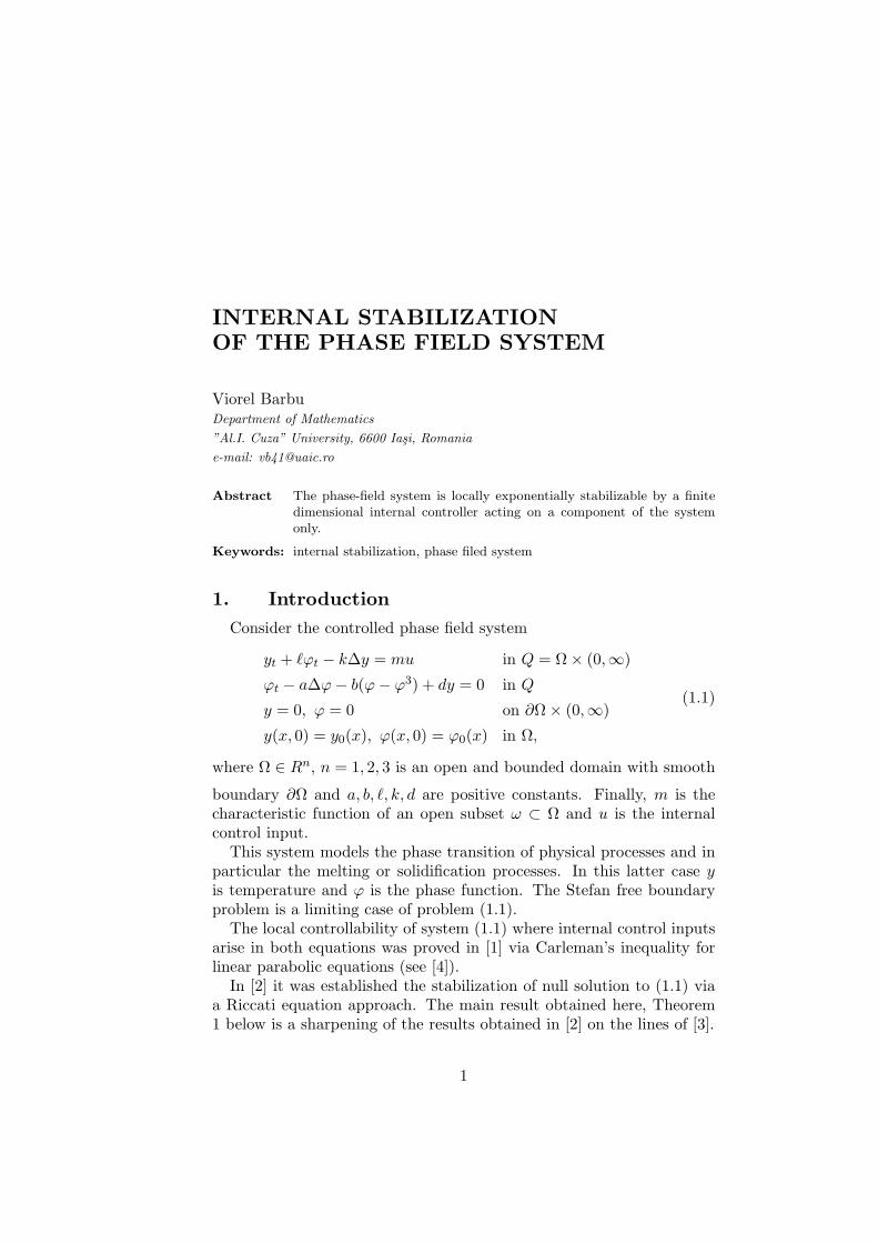
1. IntroductionConsider the controlled phase field system
yt + `ϕt − k∆y = mu in Q = Ω× (0,∞)
ϕt − a∆ϕ− b(ϕ− ϕ3) + dy = 0 in Q
y = 0, ϕ = 0 on ∂Ω× (0,∞)
y(x, 0) = y0(x), ϕ(x, 0) = ϕ0(x) in Ω,
(1.1)
where Ω ∈ Rn, n = 1, 2, 3 is an open and bounded domain with smooth
boundary ∂Ω and a, b, `, k, d are positive constants. Finally, m is thecharacteristic function of an open subset ω ⊂ Ω and u is the internalcontrol input.
This system models the phase transition of physical processes and inparticular the melting or solidification processes. In this latter case yis temperature and ϕ is the phase function. The Stefan free boundaryproblem is a limiting case of problem (1.1).
The local controllability of system (1.1) where internal control inputsarise in both equations was proved in [1] via Carleman’s inequality forlinear parabolic equations (see [4]).
In [2] it was established the stabilization of null solution to (1.1) viaa Riccati equation approach. The main result obtained here, Theorem1 below is a sharpening of the results obtained in [2] on the lines of [3].
1

2 ADVANCES IN AUTOMATIC CONTROL
2. The main resultWe set A = −∆ with D(A) = H2(Ω) ∩ H1
0 (Ω). Let ψi∞i=1 be anorthonormal basis of eigenfunctions for the operator a, i.e.,
Aψi = λiψi, i = 1, ....
(Here each eigenvalue λi is repeated according to its multiplicity.)Denote by As, 0 < s < 1, fractional powers of Q and set H = L2(Ω),
W = D(A
14
), V = D
(A
12
), with the usual norms.
For each ρ > 0 denote by Wρ the open ball in W ×W
Wρ =
(y0, ϕ0) ∈W ×W ;∣∣∣A 1
4 y0
∣∣∣2 +∣∣∣A 1
4ϕ0
∣∣∣2 < ρ2
.
Now we are ready to formulate the main result of this paper.
Theorem 1. There are N and RN : D(RN ) ⊂ H×H → H×H, linear,self–adjoint satisfying
C2
(∣∣∣A 14 y∣∣∣2+ ∣∣∣A 1
4ϕ∣∣∣2)≤ < RN (y, ϕ), (y, ϕ) > ≤C1
(∣∣∣A 14 y∣∣∣2+ ∣∣∣A 1
4ϕ∣∣∣2)
(2.1)
‖RN (y, ϕ)‖2H×H ≤ C3
(∣∣∣A 12 y∣∣∣2 +
∣∣∣A 12ϕ∣∣∣2) (2.2)
and such that the feedback controller
u = −N∑
i=1
(R11y(t) +R12ϕ(t), ψj)ωψj (2.3)
exponentially stabilizes (1.1) on Wρ. More precisely, for all (y0, ϕ0) ∈Wρ we have
|y(t)|+ |ϕ(t)| ≤ C4e−γt(‖y0‖W + ‖ϕ0‖W ) (2.4)
∫ ∞
0
(∣∣∣A 14 y(t)
∣∣∣2 +∣∣∣A 1
4ϕ(t)∣∣∣2) dt ≤ C5(‖y0‖2
W + ‖ϕ0‖2W ). (2.5)
Here RN =∥∥∥∥ R11 R12
R12 R22
∥∥∥∥ , (·, ·)ω is the scalar product in L2(ω) and
‖y‖W =∣∣∣A 1
4
∣∣∣, | · | is the norm of H. Finally, < ·, · > is the scalarproduct of H ×H.

Internal stabilization of the phase field system 3
The idea of the proof already used in [2], [3] is in few words the follow-ing. One proves first that the linearization system associated with (1.1)is exponentially stabilizable (Lemma 1) and use this fact to construct afeedback controller RN satisfying (2.1), (2.2) (Lemma 2). Finally, oneproves that controller (2.3) exponentially stabilizes system (1.1).
3. Stabilization of the linear systemsWe shall rewrite system (1.1) as
y′ + kAy − a`Aϕ− `dy + `bϕ− `bϕ3 = mu
ϕ′ + aAϕ− bϕ+ dy + bϕ3 = 0 in Q
y(0) = y0, ϕ(0) = ϕ0 in Ω.
(3.1)
Equivalently,
d
dt
(y
ϕ
)+A
(y
ϕ
)+ F
(y
ϕ
)=(mu
0
)(y
ϕ
)(0) =
(y0
ϕ0
),
(3.2)
where
A =
∥∥∥∥∥ kA− `d −a`A+ `b
d aA− b
∥∥∥∥∥ (3.3)
F
(y
ϕ
)=
(−`bϕ3
bϕ3
). (3.4)
Consider the linear control system
d
dt
(y
ϕ
)+A
(y
ϕ
)=(mu
0
)(y
ϕ
)(0) =
(y0
ϕ0
) (3.5)
i.e.,y′ + kAy − a`Aϕ− `dy + `bϕ = mu
ϕ′ + aAϕ− bϕ+ dy = 0
y(0) = y0, ϕ(0) = ϕ0.
(3.6)
We set XN = spanψiNi=1 and denote by PN the projector on XN .
We set
y = yN + zN , ϕ = ϕN + ζN ,
yN = PNy, ϕN = PNϕ, zN = (I − PN )y, ζN = (I − PN )ϕ

4 ADVANCES IN AUTOMATIC CONTROL
and rewrite system (3.6) as
yjN + (kλj − `d)yj
N − (a`λj + `b)ϕjN = (PN (mu), ψj), j = 1, ..., N,
ϕjN + dyj
N + (aλj − b)ϕjN = 0, j = 1, ..., N,
(3.7)zjN+(kλj−`d)zj
N−(a`λj+`b)ζjN=((I − PN (mu), ψj), j=N + 1, ...,
ζjN + dzj
N + (aλj − b)ζjN = 0, j = N + 1, ...,
ζN (0) = PNy0, ϕN (0) = PNϕ0,
zN (0) = (I − PN )y0, ζN (0) = (I − PN )ϕ0.(3.8)
Here
yN =N∑
j=1
yjNψj , ϕn =
N∑j=1
ϕjNψj ,
ζN =N∑
j=N+1
zjNψj , ζN =
N∑j=N+1
ζjNψj .
Lemma 1. There are yj ∈ L2(0,∞), j = 1, ..., N, such that for N largeenough the controller
u(x, t) =N∑
j=1
uj(t)ψj(x) (3.9)
stabilizes exponentially system (3.6), i.e.,
|y(t)|+ |ϕ(t)|+ |uj(t)| ≤ Ce−γt(|y0|+ |ϕ0|), ∀t ≥ 0. (3.10)
for some γ > 0.
Here | · | denotes the norm in L2(Ω).Proof. To prove Lemma 1 which is the main ingredient of the proof ofTheorem 1 we shall prove first the exact null controllability of the finitedimensional system (3.7) for N large enough.
For u given by (3.9) system (3.7) becomes
yjN + (kλj − `d)yj
N − (a`λj + `b)ϕjN =
N∑i=1
ui(t)(ψj , ψi)ω,
ϕjN + dyj
N + (aλj − b)ϕjN = 0, j = 1, ..., N.
(3.11)
The dual system of (3.7) is the following
pjN − (kλj − `d)pj
N − dqjN = 0, j = 1, ..., N,
qjN + (a`λj + `b)pj
N − (aλj − b)qjN = 0.
(3.12)

Internal stabilization of the phase field system 5
We setBN = ‖(ψj , ψi)ω‖N
i,j=1,
where (·, ·)ω, is the scalar product in L2(ω). Recall that (3.11) is nullcontrollable on [0, T ] if and only if
B∗N (pN (t)) = 0, ∀t ∈ (0, T ) (3.13)
implies thatpN (t) ≡ 0, qN (t) ≡ 0. (3.14)
By (3.13) we have
N∑j=1
(ψj , ψi)ωpjN (t) ≡ 0, i = 1, ..., N. (3.15)
On the other hand, det ‖(ψj , ψi)ω‖ = 0 because otherwise system ψjNj=1
is dependent on ω and this implies by unique continuation that ψjNj=1
is linearly dependent on Ω. Hence pN ≡ 0 and by (3.12) it follows thatqN ≡ 0. Hence system (3.11) is null controllable and this implies thatthere are ujN
j=1 (given in feedback form) such that system (3.11) isexponentially stable with arbitrary exponent γ, i.e.,
|yjN (t)|+ |ϕj
N (t)|+ |uj(t)| ≤ Ce−γt|yjN (0)|+ |ϕj
N (0)|, ∀t ≥ 0. (3.16)
Substituting (3.9) into (3.8) and taking in account (3.16) we get
12d
dt(|zj
N |2 + α|ζj
N |2) + (kλj − `d)|zj
N |2 − (a`λj + `b)zj
N · ζjN+
+αdzjNζ
jN + α(aλj − b)|ζj
N |2 = α(I − PN )(mu,ψj)ζjN ,
where α > 0 is arbitrary.For α suitable chosen (for instance for α ≥ 2a`) and N large enough
we see that
|zjN (t)|2 + α|ζj
N (t)|2 ≤ e−γN t(|zjN (0)|2 + |ζj
N (0)|2)+
+∫ t
0e−γN (t−s)
N∑j=1
|uj(s)|2ds ≤ Ce−γ1N t(|zj
N (0)|2 + |ζjN (0)|2), ∀t ≥ 0,
where γ1N > 0.
This completes the proof.Next consider the optimal control problem

6 ADVANCES IN AUTOMATIC CONTROL
Min
12
∫ ∞
0
(∣∣∣A 34 y(t)
∣∣∣2 +∣∣∣A 3
4ϕ(t)∣∣∣2 + |u(t)|2
)dt
subject to (3.7), u =N∑
j=1
uj(t)ψj
= Φ(y0, ϕ0).(3.17)
It is readily seen that
Φ(y0, ϕ0) ≤ C
(∣∣∣A 34 y0
∣∣∣2 +∣∣∣A 3
4ϕ0
∣∣∣2) ∀y0 ∈ D(A
14
), ϕ0 ∈ D
(A
14
).
(3.18)Indeed, multiplying (3.6) by A
12 y and αA
12ϕ, respectively, we get
12d
dt
(∣∣∣A 14 y(t)
∣∣∣2 + α∣∣∣A 1
4ϕ(t)∣∣∣2)+ k
∣∣∣A 34 y(t)
∣∣∣2 − a`(A
12 y(t), Aϕ(t)
)−
−`d(y(t), A
12 y(t)
)+ `b
(ϕ(t), A
12 y(t)
)+
+αa∣∣∣A 3
4ϕ(t)∣∣∣2 + α
(A
12 y(t), dy(t)− bϕ(t)
)=(mu(t), A
12 y(t)
).
For α sufficiently large we get
d
dt
(∣∣∣A 14 y(t)
∣∣∣2 + α∣∣∣A 1
4ϕ(t)∣∣∣2)+ δ
(∣∣∣A 34 y(t)
∣∣∣2 +∣∣∣A 3
4ϕ(t)∣∣∣2) ≤
≤ C(|y(t)|2 + |ϕ(t)|2 + |u(t)|2
), t > 0.
Integrating on (0,∞) and using Lemma 1 we get (3.18) as claimed.Hence there is a symmetric continuous operator RN : W × W →
W ′ ×W such that
Φ(y0, ϕ0) =12< RN (t0, ϕ0), (y0, ϕ0) > ∀(y0, ϕ0) ∈W ×W. (3.19)
We set
RN =
∥∥∥∥∥ R11 R12
R12 R22
∥∥∥∥∥ .We have also
Lemma 2. Let (y∗, ϕ∗, u∗) be optimal in (3.17). We have
u∗j (t) = −(R11y(t) +R12ϕ(t), ψj)ω, ∀t ≥ 0, j = 1, ..., N. (3.20)
Moreover,

Internal stabilization of the phase field system 7
|RN (y, ϕ)|H×H ≤ C(‖y‖+ ‖ϕ‖), ∀(y, ϕ) ∈ V (3.21)
and
< RN (y, ϕ)(y, ϕ) >≥ ω(|y|2W + |ϕ|2W ) ∀(y, ϕ) ∈W ×W. (3.22)
Finally, RN is the solution to the Riccati equation
< kAy − `aAϕ− `dy + `bϕ,R11y +R12ϕ > +
+ < aAϕ+ dy − bϕ,R12y +R22ϕ > +
+12
∣∣∣∣∣∣N∑
j=1
(R11y +R12ϕ,ψj)2ω
∣∣∣∣∣∣ ==
12
(∣∣∣A 34 y(t)
∣∣∣2 +∣∣∣A 3
4ϕ(t)∣∣∣2) , ∀(y, ϕ) ∈ D(A)×D(A).
(3.23)
The proof of Lemma 2 is exactly the same as that given in [2], [3] andso it will be omitted.
4. Proof of Theorem 1Consider the closed loop system
yt + kAy − `aAϕ− `dy + `bϕ− `bϕ3+
+mN∑
i=1
(R11y +R12ϕ,ψj)ωψj = 0
ϕt + aAϕ− bϕ+ dy = 0, t ≥ 0,
y(0) = y0, ϕ(0) = ϕ0.
(4.1)
It is easily seen that for each (y0, ϕ0) ∈ H ×H this system has a uniquesolution (y, ϕ) ∈ L2(0;T ;V ) × L2(0, T ;V ). Multiplying first equation(4.1) by R11y +R12ϕ the second by (R12y +R22ϕ) and using (3.23) weobtain after some calculation
d
dt< R(y, ϕ), (y, ϕ) > +
∣∣∣A 34 y(t)
∣∣∣2 +∣∣∣A 3
4ϕ(t)∣∣∣2 ≤ C|(R11y+R12ϕ,ϕ
3)|.
On the other hand, we have
|(R11y +R12ϕ,ϕ3)| ≤ C|R11y +R12ϕ| |ϕ|3L6(Ω) ≤
≤ C(‖y‖+ ‖ϕ‖)|ϕ|3L6(Ω) ≤
≤ C
(∣∣∣A 14 y∣∣∣ 12 +
∣∣∣A 34 y∣∣∣ 12 |ϕ|3L6 +
∣∣∣A 14ϕ∣∣∣ 12 ∣∣∣A 3
4ϕ∣∣∣ 12 |ϕ|3L6
)≤

8 ADVANCES IN AUTOMATIC CONTROL
≤ C
(∣∣∣A 14 y∣∣∣ 12 ∣∣∣A 3
4 y∣∣∣ 12 ∣∣∣A 1
4ϕ∣∣∣3 +
∣∣∣A 14ϕ∣∣∣ 12 ∣∣∣A 3
4ϕ∣∣∣ 12 ∣∣∣A 1
4ϕ∣∣∣3) ≤
≤ C
(∣∣∣A 14ϕ∣∣∣3 ∣∣∣A 3
4 y∣∣∣+ ∣∣∣A 1
4ϕ∣∣∣ ∣∣∣A 1
4ϕ∣∣∣3) ≤ C
∣∣∣A 14ϕ∣∣∣2(∣∣∣A 3
4 y∣∣∣2 +
∣∣∣A 34ϕ∣∣∣2)+
+C(∣∣∣A 3
4ϕ∣∣∣2 ∣∣∣A 1
4ϕ∣∣∣2) ≤ CΦ(y, ϕ)
(∣∣∣A 14 y∣∣∣2 +
∣∣∣A 34ϕ∣∣∣2) .
Hence for Φ(y, ϕ) ≤ ρ sufficiently small,
d
dt< R(y, ϕ), (y, ϕ) > +
∣∣∣A 34 y∣∣∣2 +
∣∣∣A 34ϕ∣∣∣2 ≤ 0.
Finally, if < R(y0, ϕ0), (y0, ϕ0) > ≤ ρ small enough we arrive to con-clusion.
References1 V. Barbu, Local controllability of the phase field system, Nonlinear Analysis, 50
(2002), 363–372.
2 V. Barbu, G. Wang, Internal stabilization of semilinear parabolic systems (to appear).
3 V. Barbu, R. Triggiani, Internal stabilization of Navier–Stokes with finite dimensionalcontrollers (to appear).
4 A.V.Fursikov, O.Yu.Imanuilov, Controllability of Evolution Equations, Lectures Notes,34(1996), Seoul University Press.

A SOLUTION TO THE FIXED END-POINT LINEAR QUADRATIC OPTIMAL PROBLEM
Corneliu Botan, Florin Ostafi and Alexandru Onea “Gh. Asachi” Technical University of Iasi Dept. of Automatic Control and Industrial Informatics Email: cbotan, fostafi, [email protected]
Abstract A linear quadratic optimal problem with fixed end-point is studied for continuous and discrete case. The proposed solution is convenient for control law implementation. Some remarks referring to the existence of the solution are indicated.
Keywords: optimal control, linear quadratic, fixed end-point, continuous-time, discrete-time
1. Introduction A completely controllable linear time invariant system is considered
x(t) Ax(t) Bu(t)= + , (1)
where nx R∈ is the state vector, mu R∈ is the control vector and A and B are matrices of the appropriate dimensions. The optimal control problem refers to the criterion
f
0
tT T
t
1J [x (t)Qx(t) u (t)Pu(t)]dt2
= +∫ , (2)
TQ Q 0= ≥ , TP P 0= > (the symbol T denotes the transposition). The problem is to find the control u(t) that transfer the system (1) from the initial state 0
0x(t ) x= to a given final state ffx(t ) x= (Anderson and
Moore, 1991; Athans and Falb, 1966). The usual case that will be considered is fx(t ) 0= . The approach for a more general case, when the target set is
fCx(t ) 0= , C∈R p×n is similar.

ADVANCES IN AUTOMATIC CONTROL
10
A similar problem can be formulated for the discrete-time case (Kuo, 1992), referring to the system x(k 1) Ax(k) Bu(k)+ = + (3)
and to the criterion
f
0
k 1T T
k kJ x (k)Qx(k) u (k)Pu(k)
2
−
=
τ= +∑ . (4)
In (3) and (4), x(k) and u(k) denote the vectors x and u at the discrete moment kτ, k Z∈ , and τ is the sampling period (we shall consider τ=1). Equation (3) can be obtained via discretization of the equation (1). It is preferred the same notations for matrices although they have, of course, different values. Since the system is time invariant, we may consider t0=0 and k0=0. The argument t or k will be omitted in the following relations if they are similar for both continuous and discrete case.
From the Hamiltonian conditions one obtains
1 Tu(t) P B (t)−= − λ , nRλ∈ , (5)
1 T
T
x(t) Ax(t) N (t), N BP B
(t) Qx(t) A (t)
−= − λ =
λ = − − λ (6)
for the continuous case and
1 Tu(k) P B (k 1)−= − λ + (7)
T
x(k 1) Ax(k) N (k 1)
(k) Qx(k) A (k 1)
+ = − λ +
λ = + λ + (8)
for the discrete case.
If the 2n-order vector x
γ = λ is introduced, the equations (6) and (8) can
be written in the form c(t) G (t)γ = γ (9) and d(k 1) G (k)γ + = γ , (10)
respectively. In the above relations
c T
A NG
Q A
− =
− − ,
T T
d T T
A NA Q NAG
A Q A
− −
− −
+ −=
− , (11)
where T 1 TA (A )− −= .

A solution to the fixed end-point linear quadratic optimal problem
11
The solution to (9)/(10) can be expressed as
0(.) (.)γ = Γ γ , (12)
where 0γ is the vector γ at the initial instant, and
11 12 2nx2n
21 22
(.) (.)(.) R
(.) (.)Γ Γ
Γ = ∈ Γ Γ , Γij ∈ Rnxn, i,j = 1,2, (13)
is the transition matrix for G. It is possible to compute γ(.) from (12) only if the initial value of the co-state vector λ is established. For this purpose, we explicit the vector x from (12)
0 02x(.) (.)x (.)11 1= Γ + Γ λ . (14)
Since fx 0= , one obtains
0 1 012f 11f x−λ = −Γ Γ , (15)
where 11f 11 f(t ,0)Γ = Γ , 12f 12 f(t ,0)Γ = Γ for the continuous case and
11f 11 f(k )Γ = Γ , 12f 12 f(k )Γ = Γ for the discrete case. This solution implies that 12fΓ is a nonsingular matrix. The conditions for non-singularity of this matrix will be discussed below. Now, the system (9)/(10) can be solved and the optimal trajectory (14) is in the two cases:
1 011 12 12f 11fx(t) [ (t,0) (t,0) ]x−= Γ − Γ Γ Γ , (16)
1 011 12 12f 11fx(k) [ (k) (k) ]x−= Γ − Γ Γ Γ . (17)
From (12) and (15) it also follows
1 021 22 12f 11f(t) [ (t,0) (t,0) ]x−λ = Γ −Γ Γ Γ , (18)
1 021 22 12f 11f(k) [ (k) (k) ]x−λ = Γ −Γ Γ Γ . (19)
The optimal control for continuous case is obtained replacing (18) in (5). For the discrete case, it has to express λ(k+1) from (8) and then use (19) and (7):
1 T T 1 T T 1 021 22 21f 11fu(k) P B A Qx(k) P B A [ (k) (k) ]x− − − − −= − Γ −Γ Γ Γ . (20)
The control vector u(k) can be computed with (20) or replacing x(k) in terms of x0 from (17). In the both cases only the open loop control is obtained. In order to obtain the closed loop control, the vector x0 is replaced in (20) from (17). But this approach implies a considerable increase of the computing difficulties, because it has to compute in real time the inverse of a time variant matrix. A similar situation also appears in the continuous case.

ADVANCES IN AUTOMATIC CONTROL
12
The method presented below avoids these difficulties. In the sequel, it will be presented only the proof for the discrete time case. For the continuous time case only the final results will be indicated. Some of these results for continuous case are indicated in (Botan and Onea, 1999).
2. Main results
2.1. Basic relations The main idea of the method is to perform a change of variable, so that one of the nxn matriceal blocks of the system matrix to be a null matrix:
(.) U (.)γ = ρ , x(.)
(.)v(.)
ρ =
(21)
with
2nx2nI 0U R
R I
= ∈
, 1 I 0U
R I− = −
. (22)
I is the n x n identity matrix and R is a n x n constant positive defined matrix. From (21) and (22) results
(.) Rx(.) v(.)λ = + . (23)
The equation for the new variables in the discrete time case is
(k 1) H (k)ρ + = ρ , (24)
where
11 121 2nx2n nxnd ij
21 22
H HH U G U R , H R , i, j 1,2
H H−
= = ∈ ∈ =
, (25)
Matrix H21 is 21 11 12 22 21H RG RG R G R G= − − + + ,
where ijG ,i 1,2= are the n x n matriceal blocks of dG . Using (11), one obtains
T T21H (I RN)A R (I RN)A Q RA− −= + − + −
or
T T 121H (I RN)A [R Q A (I RN) RA]− −= + − − + .
If we impose

A solution to the fixed end-point linear quadratic optimal problem
13
T 1R Q A (I RN) RA−= + + (26) then 21H 0= . (27)
Note that the matrix I+RN is non-singular and also that all the inverse matrices which appear in the following relations exist. One remark that (26) is the discrete Riccati equation for the LQ problem with infinite final time. Using (26), from (11) and (25) it also follows
1 T T T11 12 12 22 11H (I NR) A; H G NA ; H H (I RN)A− − − −= + = = − = = + . (28)
The transition matrix for H is k 2nx2n(k) H RΩ = ∈ . One obtains for Ω(k) a similar form as for H
11 12
22
(k) (k)(k)
0 (k)Ω Ω
Ω = Ω (29)
and
k 1
k k i k i 111 11 22 22 12 12k 11 12 22
i 0(k) H , (k) H , (k) H H H H
−− −
=Ω = Ω = Ω = =∑ .(30)
The transition matrix Γ(k) can be expressed in terms of the transition matrix Ω(k) taking into account (22), (25) and (29) and has the form:
11 12 121
11 12 22 12 22
(k) (k)R (k)(k) U (k)U
R (k) R (k)R (k)R R (k) (k)− Ω −Ω Ω
Γ = Ω = Ω − Ω −Ω Ω +Ω .(31)
The solution of system (24) is
0 0
11 120
22
x(k) (k)x (k)v
v(k) (k)v .
= Ω +Ω
= Ω (32)
The initial vector v0=v(0) results from (15) and (23) for k=0 and it is
0 1 012f 11fv ( R)x−= − Γ Γ + . (33)
Substituting (30), (31) into (33) it results
f
f
k0 1 0 1 012f 11f 12k 11v x H H x− −= −Ω Ω = − . (34)
The optimal control is obtained from (7), (8) and (23) as
1 T T 1 T Tu(k) P B A (R Q)x(k) P B A v(k)− − − −= − − − .
Replacing (32) and (34) it results

ADVANCES IN AUTOMATIC CONTROL
14
f
f
k1 T T 1 T T k 1 022 12k 11u(k) P B A (R Q)x(k) P B A H H H x− − − − −= − − + . (35)
One can remark that the optimal control can be expressed as
f su(k) u (k) u (k)= + , (36) where 1 T T
fu (k) P B A (R Q)x(k)− −= − − (37)
is the feedback component and
f
f
k1 T T k 1 0s 22 12k 11u (k) P B A H H H x− − −= (38)
is a supplementary component that depends on the initial state x0=x(0). Note that in (37) only the term 1 T Tu(k) P B A Rx(k)− −= − is a proper feedback component and it is identical with the control vector obtained in the LQ problem with infinite final time. Therefore the real time computing of the optimal control u(k) implies to establish a usual state feedback component uf(k) and a supplementary component us(k). The last one contains only one time variant element: the transition matrix k
22H , which evidently can be recursively computed. For the continuous time case, the transformed system can be written as
(t) H (t)ρ = ρ , (39)
with
1c T
F NH U G U
0 F− −
= = −
, (40)
where F A NR= − . (41)
The form (40) is obtained if we impose
TRNR RA A R Q 0− − − = , (42)
that is R satisfies the Riccati algebraic equation that appears in the continuous LQ problem with infinite final time. The transition matrix corresponding to H is
12(t, ) (t, )(t, )
0 (t, )Ψ τ Ω τ
Ω τ = φ τ , (43)
where (.)Ψ and (.)φ are the transition matrices for F and -FT, respectively and
12 t(t, ) (t, )N ( , )d
τΩ τ = Ψ θ φ θ τ θ∫ . (44)

A solution to the fixed end-point linear quadratic optimal problem
15
Since 1(.) U (.)U−Γ = Ω , one obtains
12 12
12 12
(.) (.)R (.)(.)
R (.) R (.)R (.)R (.) R (.)Ψ −Ω Ω
Γ = Ψ − Ω − φ φ + Ω . (45)
The solution to the system (39) is
0
0
x(t) x(t,0)
v(t) v
= Ω
, (46)
where 0 1 0 1 0
12f 11f 12f f f fv x x , (t ,0)− −= −Ω Ω = −Ω Ψ Ψ =Ψ (47)
with
12f 12 f(t ,0)Ω =Ω and 11f 11 f f(t ,0) (t ,0)Ω =Ω = Ψ .
From (46) and (47) it follows
1 0
12 12f f1 0
12f f
x(t) [ (t,0) (t,0) ]x
v(t) (t,0) x .
−
−
= Ψ +Ω Ω Ψ
= −φ Ω Ψ (48)
The optimal control u(t) is f su(t) u (t) u (t)= + , (49)
where the feedback component is
1 Tfu (t) P B Rx(t)−= − (50)
and the supplementary component is
1 T 1 0s 12f fu (t) P B (t,0) x− −= − φ Ω Ψ (51)
and depends on the initial state x0. As in the discrete case, the last component contains only one time variant element, namely the transition matrix (t,0)φ ; this matrix can be recursively computed.
Remark 1. It is usually desired to maintain x(t) = 0 for t > tf. For this purpose it is necessary to adopt u(t) = 0 for t > tf.
Remark 2. The performed simulation tests have indicated that a significant increase of the sampling period only for the supplementary component leads to a small difference in the system behavior. This aspect is important because offers the possibility of the decrease of the real time computing volume.

ADVANCES IN AUTOMATIC CONTROL
16
2.2 The existence of the solution As results from the previous relations, the problem has solution if the matrix
12f 12fΓ = Ω is non-singular. Indeed, one remarks from (15) that there is a unique initial vector 0 (0)λ = λ for a given 0x x(0)= if the matrix
12f 12 f(t ,0)Γ = Γ is non-singular and then the formulated problem has solution. The condition for non-singularity of the matrix 12fΓ is given by the following
Theorem If the pair (A,B) is completely controllable, then matrix 12fΓ is non-singular.
Proof. For the continuous time case, from (31) and (44) one obtains
f
Tf f
tF(t ) F (t )1 T
12 f 12 f f0
(t ,0) (t ,0) e BP B e d (t ,0)−θ −θ−Γ = Ω = − θφ∫ . (52)
Since the transition matrix f(t ,0)φ is non-singular, 12 f(t ,0)Γ is non-
singular if the matrix Tft F 1 T F
f 0(t ,0) e BP B e dσ − σΠ = σ∫ is non-singular. One
can prove (Botan, 1991) that f(t ,0) 0Π > if (A,B) is completely controllable and thus the theorem is proved. For the discrete time case, the proof is similar, but some supplementary transformations are necessary because the matriceal block
T n12H NA R−= − ∈ of the matrix 2nx2nH R∈ contains the factor A–T.
Firstly, we will establish another expression for the matriceal blocks Hij, i,j=1,2, given by (28). From (28) one obtains
1 1 111H A (R N)R− − −= + . (53)
Let us denote the matrix
1 1 1 1 TX R N R BP B− − − −= + = + . (54)
Multiplying (54) with X and then with R, it results
1 TR X XBP B R−= + . (55)
Multiplying (55) with B, one obtains
1 TRB XBP (P B RB)−= + .
This relation is multiplied with T 1(P B RB)−+ , then with TB R and then we subtract from R:
T 1 T 1 TR RB(P B RB) B R R XBP B R− −− + = − . (56)

A solution to the fixed end-point linear quadratic optimal problem
17
Let us denote TP P B RB= +
1 TN BP B−= . (57)
Using these notations and (55), relation (56) becomes
X R RNR= − . (58) From (54) and (58) one obtains
1 1(R N) R RNR− −+ = − (59) and then 1 1 1
11H R (R N) A (I NR)A− − −= + = − (60)
or
11H A BK F= + = , 1 TK P B RA−= − . (61)
From (28) one obtains
T T22 11H H F− −= = , (62)
T T T T T T T T12H NA NA F F NA A (I RN)F (N NRN)F− − − − − −= − = − = − − = − − .
But from (59) it follows N NRN N− = , so that
T12H NF−= − . (63)
Having in view (61), (62) and (63), the matrix H can be written in the form
T
T
F NFH
0 F
−
−
−=
.
Now we introduce the nonsingular matrix
T
I 0
0 F−
χ =
and carry out the transformation
1T
F ND H
0 F−
−
−= χ χ =
and analogous for the corresponding transition matrix
11k 12k1
2k(k) (k)
0− ∆ ∆
∆ = χΩ χ = ∆ , (64)

ADVANCES IN AUTOMATIC CONTROL
18
k11k F∆ = , T k
22k (F )−∆ = , k 1
i k i 112k 11 12 22
i 0D D D
−− −
=∆ =∑ .
For k=kf
ff
ff f
k 1k 1i i
12f 12 f 11 12 22 22i 0
k 1k 1 k 1i T i T T
i 0
(k ) D D D D
F N(F ) (F ) (F ) ,
−−−
=−
− −− −
=
∆ = ∆ = =
= − = −Π
∑
∑ (65)
where
fk 1
i 1 T i T
i 0F BP B (F )
−−
=Π = ∑ .
We shall prove now that Π is a positive defined matrix (Π>0) if the pair (A,B) is completely controllable. Indeed, if (A,B) is controllable, (F,B) is controllable, with F=A+BK. Since P>0 and R>0, P given by (57) is also positive defined, and also 1P 0− > ; in this case, there is a unique positive defined matrix V such as T 1VV P−= . We can express
fk 1
i T i T
i 0F BV(BV) (F )
−
=
Π = ∑
n 1 n 1V
[BV FBV ... F BV] [B FB ... F B] ...V
− − =
.
Since the last matrix is nonsingular and n 1[B FB ... F B]− is of rank n, the matrix n 1[BV FBV ... F BV]− is of the same rank, thus the pair (F,BV) is completely controllable and the matrix Π is positive defined. Since F-T is nonsingular, from (65) it follows that 12f∆ is nonsingular. From the transformation (64) we obtain T
12f 12f F∆ = Ω . Since 12f∆ and FT are nonsingular, 12fΩ is nonsingular and 12f 12fΓ = Ω is nonsingular and the theorem is proved also for the discrete case.
3. Simulation results Some simulation tests were performed for different conditions and different weight matrices in the criterion for both continuous and discrete case. The results presented bellow refer to a continuous system (1) with

A solution to the fixed end-point linear quadratic optimal problem
19
0 20 0
A , B3.5 19 6
= = − −
and to the criterion (2) with Q = diag (1, 3) and P=p=0.7. The corresponding matrices obtained via discretization were adopted for the discrete case. The sampling period is τ=0.002 s. The terminal moments are t0=0 and tf=0.3 s (and corresponding kf=150). The initial state is x(t0) = [50 0]T .
0 0 . 05 0. 1 0 .1 5 0 .2 0 .2 5 0 . 3-4 0
-3 0
-2 0
-1 0
0
1 0
2 0
3 0
4 0
5 0
x 1
x 2
u
Figure 1. The behavior of the system for continuous and discrete cases
Figure 1 presents the behavior of the system for both continuous and discrete cases; one can remark that the curves are practically the same in the two cases. The more significant differences between continuous and discrete case appears if the sampling period is increased. Figure 2 presents the same situation for the discrete case, but indicates in addition the behavior for k>kf, when the control u(k)=0 is adopted (see Remark 1).
0 0 .0 5 0 .1 0 .1 5 0 .2 0 .2 5 0 . 3 0 . 3 5 0 . 4-4 0
-3 0
-2 0
-1 0
0
1 0
2 0
3 0
4 0
5 0
x 1
x 2
u
Figure 2. The behavior of a system before and after the final time
Figure 3 presents a comparison between the basic discrete case and the case when the sampling period τ was increased by ten times only for the

ADVANCES IN AUTOMATIC CONTROL
20
supplementary component (see Remark 2); one can remark that the differences are not significant, especially referring to the states variables.
0 0 . 05 0. 1 0 .1 5 0 .2 0 .2 5 0 . 3-4 0
-3 0
-2 0
-1 0
0
1 0
2 0
3 0
4 0
5 0
x 1
x 2
u
Figure 3. The effect of the sampling period increase for the supplementary component
It was performed a comparison with the similar linear quadratic problem but with free end-point. The difference is that in the last case the state vector does not arrive in zero at the final time, but the control variable is significantly smaller.
4. Conclusions The linear quadratic optimal problem for continuous and for discrete case is studied; the results are presented especially for the discrete case. A new method is presented and it is obtained a very convenient form for the feedback optimal control law. Some considerations about the existence of the solution are presented. The theoretical and simulation results indicate a similarity between the continuous and discrete time cases.
References Anderson, B.D.O., and J.B. Moore (1990). Optimal Control, Prentice-Hall, New Jersey
Athans, M, and P.L. Falb (1966). Optimal Control, McGraw Hill, New York.
Botan, C. (1991) On the Fixed End-Point Linear Quadratic Optimal Problem. In: Proceedings of the 8th International Conf. on Control Systems and Computer Science. Polytechnic Inst. of Bucharest, pp 100-105, Bucharest.
Botan, C. and A. Onea (1999) Fixed End-Point Problem for an Electrical Drive System. In: Proceedings of the IEEE International Symposium on Industrial Electronics, ISIE’99, Bled, Slovenia, Vol. 3, pp. 1345-1349.
Kuo, B.C. (1992) Digital Control System, Saunders College Publishing, Philadelphia.

PATTERN RECOGNITION CONTROL SYSTEMS – A DISTINCT DIRECTION IN INTELLIGENT CONTROL
Emil Ceangă and Laurenţiu Frangu University "Dunărea de Jos" of Galaţi Str. Domnească 111, 2200 Galaţi, Romania E-mail: [email protected]
Abstract This paper presents an alternative approach of intelligent control: the pattern recognizing systems. The main idea is to endow the control system with the ability to learn from the experience generated by the interaction with the environment (the control object and the external world). Learning implies generalization and abstraction, through recognition of synthetic entities, which concentrate the essence of the past experience. The notions allowing learning, used in this approach, are called "control situations". The historical evolution of these notions is briefly exposed and they are analytically defined. Some results of the authors, presented in the paper, concern: the usefulness of each control situation in the hierarchical structure of intelligent control, the properties of the clusters, the learning automaton and the connections with other control techniques. For illustrating the approach, some applications of the pattern recognition control systems are presented.
Keywords: intelligent control, pattern recognition, control situations, hierarchy, adaptive control, strategy
1. Introduction A fundamental property of the intelligent control systems is their ability to extract, through learning, the relevant information from the environment. This action implies generalization and abstraction, which are frequently performed through pattern recognition (PR).

ADVANCES IN AUTOMATIC CONTROL
22
The use of the PR methods, in the space of the observations on the controlled process, started at the end of the '50s [Widrow, 1962, 1964]. A remarkable application of this period was the pattern recognition control system (PRCS) for an inverted pendulum; the neural learning automaton was built using the technology of those years (memistors). PR techniques for control purposes were also used in [Taylor, 1963], [Waltz and Fu, 1966]. In the paper [Nikolic and Fu, 1966], a milestone in the field, the control of a dynamic system with unknown properties is performed by a PRCS. Learning is driven by an uncertain teacher, who learns simultaneously with the PR controller. The paper presents the first theoretical and qualitative results, regarding the convergence of the learning processes. In some papers of the '60s, the generic term of "situation" was used instead of "pattern", having the meaning of an abstract entity, relevant for the control and diagnosis of the systems. The term was mainly adopted by the researchers in the field of automatic control, such as Aizerman, in the papers that theoretically founded the method of potential functions [Aizerman et al., 1965, 1966]. A refinement of this concept appears in the papers [Drăgan and Ceangă, 1968], [Ceangă, 1969a, 1969b], [Ceangă et al., 1971a, 1971b]. A paper that had an important influence on the evolution of the intelligent control is [Saridis, 1979]. Saridis revealed that intelligent systems are able to perform behavioral learning, i.e. they classify the information and take decisions through PR. This means that the intelligent systems perform generalization, through learning, in order to recognize some synthetic concepts, concerning the environment they are interacting with. The detailed description of such synthetic concepts, referred to with the generic term of "control situations", was approached in [Ceangă et al., 1981, 1984, 1985a, 1985b, 1991]. Recent papers, like [Seem and Nesler, 1996], [Ronco and Gawthrop, 1997a, 1997b], [Grigore, 2000], [Frangu, 2001], make use of the PRCS, in neural implementation. In general, the present approaches in intelligent control (including the PRCS approach) aim at the analogy with the human mind: [Frangu, 2001], [Truţă, 2002]. In the above mentioned papers, the PR techniques are used to form abstract concepts, hierarchically structured, according to the principle "Increasing Precision on Decreasing Intelligence" (IPDI) [Saridis, 1988, 1989]. The purpose of this paper is to present some recent results of the authors in the field of PRCS. The connections with previous results are also mentioned, in order to highlight algorithms and techniques that maintain their up-to-dateness. By structuring in a hierarchy the concepts of control situations, it will become clearer how PRCS perform the essential functions of the intelligent systems. According to Albus ([Albus, 1991]), these are: perception, model of the world, value judgment and behaviour generation. Some unsolved aspects will also be presented; in the opinion of the authors, they are important for the evolution of the field.

Pattern recognition control systems. A distinct direction in intelligent control 23
2. Control situation approaches Let us consider a control structure, such as that presented in figure 1, where the controlled process is a sampled dynamic system, with unknown or partially known properties. The particular variants of the generic concept of "Control Situation" depend on the function performed by the PRCS. They are described in the sequel.
Figure 1. Control of the process, through the learning PR system
1. Output situation. Let yi, i=1,...,p, y ∈ Yd, be the discrete values of the output variables, out of the set Yd of admissible values, which represent significant effects of the input variables v (measurable disturbance) and u (command). It is called output situation the set Si of the variables observed from the "environment", w, that determine the discrete value yi of the output, according to f, the causal input-output relationship of the controlled process:
; ; diif
i YyywwS ∈→= . (1)
Let ),(),...,1(),(),...,1([)1( ba nktuktuntytytw −−−−−−=−
( 1),..., ( )]Tcv t k v t k n− − − − (2)
be the vector of the observations from the environment, which is used to predict the value y(t), where k is the dead time. The output situation Si is:
)( ;)]()1([)()]1([ );1( djijj
i YtytytwytytwyMintwS ∈−−=−−−= .(3)
The membership of the vectors, with respect to the output situations, is given by the data recorded in the process (the discrete value of the output, at the moment t). For this reason, a supervised learning is possible, requiring no human teacher. The recognition of the output situations may be used for the

ADVANCES IN AUTOMATIC CONTROL
24
predictive evaluation of the effects of the commands addressed to the controlled process. 2. Command situation. Let us assume there are p admissible values of the command input. They form the set Ud of the discrete admissible commands: ui, i=1,...,p. Using the output, the command and the measurable disturbances, the vector of observations is defined:
a b c( ) [ ( ),..., ( 1), ( 1),..., ( ), ( ),..., ( )]Tz t y t y t n u t k u t k n v t k v t k n= − + − − − − − − − ,(4) where na, nb and nc are finite integers and k is the dead time (expressed in sampling periods). The learning system has to make use of the "experience" accumulated up to the moment t, with the purpose of determining the function that assigns to any vector of observations, z(t), the discrete command, ui(t), i=1,...,p, that maximizes the indicator Φ. It is called command situation the set Si of the vectors z, for which the discrete command ui is optimum, regarding the fulfillment of the objective:
),,(),(Max: djijj
i UuzuzuzS ∈Φ=Φ= . (5)
Consequently, to determine the control law means to deduce, through learning, the discriminant functions of the command situations Si. The essential problem is to build the teacher of the PR controller. In some cases, the teacher may be a human expert or a decision system, based on pre-existing control systems. However, in the general case, the teacher can be a predictor that recognizes output situations. Teaching the teacher and teaching the controller are performed simultaneously, in the frame of a dual control procedure. This one will be presented with the assumption that k=0, in order to simplify the expressions. At the current moment, j, the following operations are performed: a – The generation of a first approximation of the current command by recognition of the command situation. The reference for the next moment, j+1, is already known: )1( +jyr . The vector
( ) [ ( 1), ( ), ..., ( 1), ( 1), ..., ( ), ( ), ..., ( )]Tr a b cz j y j y j y j n u j u j n v j v j n= + − + − − − (6)
will be assigned (by recognition) to one of the classes cci piS ,...,1 , = . Let
suju =)( , ds Uu ∈ , be the discrete command associated to the recognized command situation. The recognition controller did not yet learn, so the chosen command su is considered to be the answer of the "student" that has to be compared to that of the "teacher". b – Based on the experience accumulated up to the current moment, j, the predictor recognizes output situations. It assigns the vectors

Pattern recognition control systems. A distinct direction in intelligent control 25
( ) [ ( ),..., ( 1), , ( 1),..., ( ), ( ),..., ( )]Ti a i b cw j y j y j n u u j u j n v j v j n= − + − − − (7)
( 1,..., c i p= ) to the classes okS , opk ,...,1= , corresponding to the discrete
values ky of the prediction )1(ˆ +jy . Making use of these predictions, the answer of the teacher is determined, according to the decision rule:
mrmrii
ujujyjwyjyjwyMin =⇒+−=+− )(||)1())((||||)1())((|| . (8)
c – The responses of the PR controller ( csSjz ∈)( , that is suju =)( ) and
of the teacher ( muju =)( ) are used for enriching the instruction set of the controller and for teaching it. d – The command muju =)( is effectively applied to the process and the response )1( +jy is recorded. This response is used to enrich the instruction set of the teacher, for predicting the output situations. The PRCS can be applied to controlled processes having unknown, nonlinear (possible variant) dynamics, whose objective is to minimize a quadratic criterion ([Ceangă et al., 1984, 1985a]. It can have the expression:
/)())()(( 22 ttukyktyEJ r ρ+−+= , (9)
where ρ is a weighting factor for the command effort. As previously, the block for the evaluation of the objective fulfillment (see figure 1) contains a PR predictor. This one recognizes the output situations and teaches the learning controller, that recognizes the command situations. 3. Adaptation situation. Let us consider an environment that changes its properties slowly. The fulfillment of the control objective requires the use of a control law
))(( tzu Ψ= , (10) where z(t) is defined by (4). The command (10) corresponds to particular properties of the controlled process. When the environment evolves, it is necessary to adapt the control law, by a finite number of adjustments,
)]([ zAi Ψ . The efficiency of the control law is determined by a set of measurable variables that form the "influence" vector, q. It is called adaptation situation ([Ceangă et al., 1991]) the set Si of vectors q, corresponding to the particular adjustment of the control law, Ai(.), which allows maintaining the control efficiency:
]),([]),([ : qzAqzAMaxqS ikk
i Φ=Φ= . (11)
Adaptation through recognition of such situations belongs to the family

ADVANCES IN AUTOMATIC CONTROL
26
of multi-model techniques ([Narendra and Balakrishnan, 1997], [Dumitrache and Mărgărit, 1999]). It represents an alternative to the classical adaptive control solutions, which frequently require complex and risky recursive computations. 4. Strategic situation. Let us consider a control system that can use, depending on the properties of the environment, more control strategies:
( ) ( ( )), 1,...,jju t T z t j r= = , (12)
where the function Tj(.) defines the j-th command strategy and z(t) is the vector of observations (for instance, that in (4)). It is called a strategic situation (from [Ceangă, 1969a, 1985b]) the set of vectors of observations z(t), corresponding to the best control strategy, out of the r possible strategies:
))](([))](([max /)( tzTtzTtzS jkk
j Φ=Φ= , (13)
where Φ(.) measures the fulfillment of the objective. The strategic situations may be defined mainly for complex systems, having various interactions and constraints, such as the biotechnological, economical or production systems. Every strategy concerns a particular tactical objective, which temporary gets the priority in order to fulfill the global objective. 5. Diagnosis situation. The behaviour of the dynamic systems may be evaluated by a set of indicators, called local criteria, which can make use of discrete information extracted by PR techniques. A global evaluation criterion may also be added, for the entire system. Let r be the vector of local criteria. It is called diagnosis situation the set of vectors in the space of local criteria, corresponding to a particular global evaluation of the controlled process. Some examples of discrete evaluations, defining the diagnosis situations, are: "admissible", "warning situation i", "emergency situation j", "damage regime", etc., where i or j have particular meanings for the supervised process. Figure 2 presents the hierarchical structure of a control system, based on control situations recognition (adapted from [Saridis, 1989]). Every hierarchical level requires the fulfillment of a different objective, expressed in concepts with different levels of abstraction. The abstraction level increases along with the hierarchy level because, according to the IPDI principle, superior levels do not require precision. The elimination of the details (reducing the entropy) may be performed by processes similar to those implied by the formation of general concepts, starting from a set of less general ones. In the following two chapters, the reasons for using PRCS and their particular learning algorithms will be presented separately, for the execution level and for the upper levels.

Pattern recognition control systems. A distinct direction in intelligent control 27
Figure 2. Hierarchical structure of a control system, recognizing control situations
3. Control situations for the upper hierarchical levels
3.1. Systems based on control situation recognition The control techniques based on adaptation, strategic or diagnosis (supervision) situations are already used in some papers. They appear explicitly or implicitly (that is, without using the terms introduced in this paper). A. The control structures that make use of the adaptation situation recognition have the advantage of a fast adaptation of the controller. [Frangu, 2001] presents two applications where the structure of adaptation through situation recognition corresponds to that in figure 3. Let
Xxntutuntytytx Tba ∈−−+−= ,)](),...,1(),1(),...,([)( , (14)
be the vector of observations, assigned by the recognition automaton to one of the adaptation situations , 1,...,a
iS i p= . The result of the classification aims at selecting the best fit controller, according to the recognized situation. In one of the mentioned applications, the controlled object is an elastic mechanical transmission, built at Laboratoire d'Automatique de Grenoble (figure 4). It is used as benchmark for robust and adaptive control techniques, in [Landau et al., 1995]. Depending on the mechanical load, the multiresonant frequency response modifies considerably its shape (figure 5).

ADVANCES IN AUTOMATIC CONTROL
28
This behaviour limits the performances obtained by robust and adaptive control techniques. Instead, the recognition of the adaptation situation is proposed.
Figure 3. Pattern Recognition Adaptation Structure (analogous with gain-scheduling)
Figure 4. Structure of the position control system
Figure 5. Frequency response of the controlled system, for three different dynamics
The vector of observations is:
Ttututytytytytx )]3(),2(),3(),2(),1(),([)( −−−−−= (15)

Pattern recognition control systems. A distinct direction in intelligent control 29
and the classification algorithm is based on the minimum distance to the prototypes of the classes. In addition, the selection automaton requires a supervisor, based on diagnosis situation recognition. When the supervisor detects the stationary regime, it doesn't allow the controller switching (the adaptation situations overlap in this regime, so the selection automaton runs out of information, as in any identification problem, when the identified dynamic object lacks excitation). In [Ronco, 1997a, 1997b] a "Local Model Network" (LMN) structure is used. It contains local linear models and corresponding local controllers, one pair for each functioning regime of the process. The recognition of the local model and, implicitly, that of the controller, is based on the vector Φ∈Φ X , which is part of the vector of observations (14). Within this method, the adaptation situations correspond to a pre-established partition. The recognition is performed by a set of RBF neurons, centered in a uniform net of points of ΦX . A different approach, proposed in [Jordan and Jacobs, 1994], is called "Adaptive Mixture of Experts". Here, the partition of the space ΦX is performed through learning, by a multilayer perceptron. Consequently, the domains of the classes (adaptation situations) are not equal, but depend on the approximation ability of each local model. B. The idea of switching the strategies, which justifies the concept of strategic situation, assumes that the current control objective can change, during the control of the process. The objective can change as a result of the evolution of the subprocesses (for instance: changes in behaviour, failure of the local control loops or even failure of the superior level) or of the interaction with the higher organized environment (for instance: human). This change can require to switch the controller, at the execution level, or to switch the method for the coordination of the subprocesses, at the middle (coordination and adaptation) level. Intuitively, the strategies may be switched through instructions like: "switch to a survival strategy, because a local loop is temporarily unavailable", "switch from cooperation with other agents to competition", "switch from stimulation of the bioreactor population to the rejection of the parasitic population", "switch from emergency medical care to the convalescence recovery method". The corresponding switching decisions may belong to the upper level (organization and scheduling) or to the middle level. There already are some well grounded papers, which investigate the properties of such systems, possibly in uncertain conditions. Among these, [Kuipers, 1994] studies the validation of heterogeneous control laws and [Johansson, 1996, 1997] present an analysis method for the stability of the heterogeneous controlled systems, regardless the type of the controller. The method makes use of piecewise defined Lyapunov functions, one for each validity domain of local controllers. The result obtained in this approach is also useful for the analysis of the systems based on adaptation situation and strategic situation recognition.

ADVANCES IN AUTOMATIC CONTROL
30
Among the problems raised by the heterogeneous command, those concerning the switching decision lead to using a strategic situation recognition automaton. The advantages of including such a subsystem are: - The automaton is a learning one, meaning it has the ability to learn from the examples, including unsupervised learning. In this variant, the recognition decision requires no information provided by the human expert, but uses the similarity of the examples, based on a measure of the objective's fulfillment. - It can model complex discrete approximation functions, whose analytical computation may be unreachable. To materialize these functions, both classical recognition algorithms and discrete output neural networks can be used. A simple example of using the strategic situations is presented in [Frangu, 2002], starting from the known benchmark, the “backer truck”. Obviously, there are initial positions of the truck who don’t accept solutions, such as the positions where the backside of the truck faces the wall, at low distance (figure 6). If starting from these positions, the backwards docking fails, regardless the chosen controller. In order to find out whether the initial position allows a solution or not, a recognition automaton will learn from the experience accumulated during the previous docking attempts (including the unsuccessful ones). The objective of the automaton is to predict if the current controller succeeds to dock, using the information of the initial position. If the automaton predicts the failure, the control system has to switch to a controller having a different objective than immediate docking (in this case, to drive forward, to the distance that allows secure docking).
Figure 6. Docking with start from initial positions (2, 1, 0) and (2, 1, π/2)
The initial position contains the truck backside coordinates: x (along the wall), y (distance to the wall) and orientation angle with respect to the wall, θ. Figure 6 presents two docking attempts, whose initial coordinates x and y are identical, but presenting different initial angles and different docking results. The vector of observations is the initial position:
Tyxz ],,[ θ= . (16)
The strategic situation to be recognized is the success or failure of the docking process, starting from that initial position. Using simulation

Pattern recognition control systems. A distinct direction in intelligent control 31
experiments, the learning set was formed. The data structure analysis showed that the boundary between classes has not a simple shape. Consequently, the classification was made through the potential functions method [Aizerman, 1964]. C. The diagnosis (or supervision) situations are currently used to diagnose the systems. However, the field of using the diagnosis situations is even larger (for instance, the detection of the stationary regime, in [Frangu, 2001]). In [Bivol et al., 1976], a complex energetic boiler plant, which includes more interconnected control loops, is considered. The evaluation of the quality of the dynamic regimes of the system considers more local criteria in the individual control loops, such as: overshot, damping factor, etc. The diagnosis situation called “normal” is defined in the space of local criteria, based on a recorded set of states, previously diagnosed by human operators. An automaton learns to recognize this situation and its opposite; it will be used to real-time diagnosis of the plant. On the other hand, each diagnosed state is associated to the known vector of parameters of the multivariable controller. Through learning, the situation “normal” in the space of local criteria is assigned to a domain defined in the space of parameters. The discriminant function of this domain may be understood as the membership function of the fuzzy set “normal”, in the space of parameters. It is used to solve the problem of optimization with constraints in the space of parameters (during the design stage).
3.2. Clusters' anatomy and learning algorithms In the case of adaptation situations, the data structure is similar to that of the output and command situations (will be analyzed next section). In the case of strategic and diagnosis situations, the data structure can be complex, with unconnected clusters, etc. Consequently, strong and general recognition methods, able to work with poor initial information, are necessary. One of these is the potential functions method, developed in the '60s by the team of Aizerman [Aizerman, 1964], at the Control Institute of the Moscow Academy. The adaptation and use of this method to the recognition of control situations appeared in [Drăgan and Ceangă, 1968], [Ceangă, 1969b]. The method is based on memorizing the "alien prototypes" or "poles", i.e. the vectors differently classified by the PRCS and by the teacher. A potential function ),( xxK is assigned to each of the memorized poles, x . Despite its generality and efficiency qualities, the method of potential functions cannot be used when the structure of clusters changes in time, because the adaptation of the discriminant functions would indefinitely increase the number of memorized poles. This drawback was noted in [Ceangă, 1969b] and two new recognition structures were proposed. They are also based on potential functions; they preserve the general character of

ADVANCES IN AUTOMATIC CONTROL
32
the initial method and provide the ability of adapting to slow changes of the data structure. The first method, called the method of floating poles ([Ceangă, 1969b]), contains a first stage of pre-learning, using the method of potential functions for the configuration of the learning system structure. In this stage, M poles are memorized. They mainly lie near the boundaries of the classes, where the recognition automaton is usually wrong. The continuation of the learning and the adaptation of the PRCS to the changes in boundaries are performed by adjusting the position of the poles, according to the "floating poles algorithm (FPA)". Essentially, this algorithm is similar to that presently used by the Kohonen neural networks. In the second method, presented in [Ceangă, 1969a, 1969b], [Bumbaru, 1970], the potential functions form the input layer of a recognition automaton (during the next decade, the structure was called RBF, when it was implemented by neural networks). As in the previous case (FPA), a first learning stage is used, when the poles xj, j = 1, M, are memorized. The poles are assigned the potential functions K (xj, x), j = 1, …, M, which form the input layer of the recognition automaton. During the second stage, the learning implies adjusting the weights of each potential function. In many papers, strategic and diagnosis situations are implicitly recognized, using neural networks (such as multilayer perceptrons). The drawback of the neural networks is the lack of transparency (no explanation about the clusters is provided). The advantage of the presented methods (disregarding the classical or neural implementation) consists in the selection of relevant poles; their position suggests the structure of the clusters, without disturbing the properties of generality and efficiency of the recognition algorithm.
4. Control situations for the execution level
4.1. Arguments for using recognition systems at the inferior level
In order to prove that controllers who recognize output and command situations are suitable, the informational approach for intelligent systems is useful. The concepts introduced by Saridis in [Saridis, 1989] (machine intelligence, knowledge flow, etc.) are used in [Frangu, 2001] to demonstrate the following property: for a system with a known level of uncertainty, there is a limit of the resolution of the discrete command, beyond which the entropy of the knowledge flow cannot increase. The same property applies to the recognition of discrete values of the output. Some practical examples, involving uncertainty, are presented in the sequel.

Pattern recognition control systems. A distinct direction in intelligent control 33
1. The actuator is, in most cases, the lowest precision element of a control loop. Excepting some particular cases, this affects the precision of mechanical positioning in the industry processes. Because of the important uncertainty, adopting a discrete set of values for the command becomes natural. If the distance between the discrete values is comparable to the uncertainty level, this operation does not lower the positioning precision.
2. The reference of the loops is often chosen according to uncertain technological requirements. In this case, maintaining the controlled object within the boundaries determined by the uncertainties of the reference is a satisfactory objective.
The two mentioned examples are also reasons for another modern control approach: hybrid systems, with continuous/discrete interface (HSCDI, [Antsaklis, 1994]). The comparative analysis of the two approaches in [Frangu, 2001] (PRCS and HSCDI) led to the following conclusions:
1. In HSCDI the partition is applied to the state space of the controlled object; the PR approach is based on the partition of the space of observations (see section 2).
2. The HSCDI approach requires the analytical state model of the controlled process, whereas the PR approach considers this model partially or totally unknown.
3. The synthesis of HSCDI requires the partition chosen by the human designer; the PRCS do not require predefined boundaries, because these result by learning.
4. There is not much knowledge about how to choose the partition of the continuous state space, in HSCDI. The number of discrete states is not equal to that of the discrete commands. This raises some particular problems, such as: how to determine the resolution of the partition, how to determine the masked states and absorbing states, etc. ([Oltean, 1998]). In PRCS, the number of classes is equal to the number of discrete commands, but the classes may contain more clusters. The learning solves this problem, assigning the same command to the clusters belonging to a class.
5. The HSCDI synthesis requires a complex sequence of design operations. Instead, the PR approach determines by learning the function that assigns the vectors of observations to the discrete commands.
4.2. Clusters' anatomy and learning algorithms The clusters' structure for the output and command situations have a stripe-like shape: the clusters lie in compact and adjacent domains of the space of observations, with similar boundaries. There is an order of the clusters, corresponding to the order of the discrete values of the variable that

ADVANCES IN AUTOMATIC CONTROL
34
generated the classes (the output or the command input). Some of the observed properties of the clusters are mentioned in [Frangu, 2001] (some of them are even demonstrated, for Hammerstein type systems). Among these:
- if the controlled system is linear, the boundaries of the clusters are parallel hyperplanes, the clusters are adjacent and disposed in order;
- the boundaries may be hyperplanes even for a larger class of nonlinear systems; to illustrate this property, four examples are presented in figure 7a-d, in a two-dimensional space of observations; the structure 7b appeared in a control problem for a biotechnological process, developed in a bioreactor [Frangu, 2001a];
- if the system does not contain hysteresis or discontinuous functions, every cluster is connected; in the contrary case, the clusters may become unconnected, subjects of some sort of space shearing (fig. 7c);
- there is a unique curve in the space of observations, which corresponds to the stationary regime and crosses all the classes; the low frequency excitation of the controlled process determines observation vectors lying in the neighborhood of this curve, whereas the vectors determined by a richer dynamics of the process are situated farther;
- if the noise disturbing the output is zero averaged, the boundaries obtained by learning converge to cluster’s true position, even if the noise is not white.
For the presented types of clusters, the appropriate recognition algorithms are those based on the minimum distance with respect to the skeleton of the clusters. If the boundaries are linear, the skeleton is the own regression line, obtainable through batch processing, which has guaranteed convergence.
a b c d
Figure 7. Possible shapes of the clusters, for the output situations
5. Conclusions and new research directions Intelligent control implies generalization and abstraction operations, which lead to synthetic concepts, necessary for operating in uncertain conditions or for the superior levels of the hierarchical control structure. These operations are performed through learning and aim at forming patterns with different levels of abstraction. In this work, the patterns generically called “control situations” are: output, command, adaptation, strategic and

Pattern recognition control systems. A distinct direction in intelligent control 35
diagnosis situations. They allow obtaining solutions of the control problems through situation recognition, in classical or neural implementation. Some of them are illustrated in the paper. Some new research directions in PRCS, in the opinion of the authors:
1. The investigation of the systems' stability, when the recognition of the adaptation situation determines the switching of the control laws or of their parameters. Considering this approach as a more general multimodel method can be the starting point [Ronco, 1997a, 1997b].
2. The investigation of the structure in figure 1, where a PR system is taught to recognize command situations, by a learning teacher, who recognizes output situations (teaching the controller by an uncertain teacher). The beginning was made by Nikolic and Fu, in 1966, when they analyzed the convergence of the learning algorithms, for the controller and for the uncertain teacher, but for a particular variant of the problem.
3. Reconsidering the PRCS approach, according to [Goertzel, 1993], where a new mathematical model of the intelligence is proposed. It integrates specific operations, like perception, induction, deduction, analogy, etc., within a network (the "master network") that operates with patterns. Induction is defined as “the construction based on the patterns recognized in the past, of a coherent model of the future”. The perception is introduced as “the network of pattern recognition processes through which an intelligence builds a model of the world” and “the perceptual hierarchy is composed of a number of levels, each one recognizing patterns in the output of the level below it”. Deduction is also introduced by pattern recognition theory. Based on the previous concepts, “intelligence is defined as the ability to optimize complex functions of unpredictable environments”. The theoretical framework of Goertzel’s model of mind can generate new ideas and research directions in the field of intelligent control.
References Aizerman, M.A., Braverman, E.M., Rozonoer, L.I. (1964) Teoreticeskie osnovy metoda
potentialnyh functii i zadace ob obucenii avtomatov raspoznovaniiu situatii na classy, Avtomatika i Telemehanika, 1964, 25, pp. 917-937.
Aizerman, M.A. (1965) Zadacia ob obucenii avtomatov razdeleniiu vhodnyh situatii na klassy (raspoznavaniiu obrazov) II IFAC Diskretnye i samonastraivaiushcesia sistemy, Iz. Mir, Moscow.
Aizerman, M.A., Braverman, E.M., Rozonoer, L.I. (1966) Problema obuceniia mashin raspoznavaniiu vneshnih situatii, Samoobuciaiushciesia avtomaticeskie sistemy, Moscow.
Albus, J.S. (1991). Outline for the theory of intelligence. IEEE Transactions on Systems, Man and Cybernetics, 21.

ADVANCES IN AUTOMATIC CONTROL
36
Antsaklis, P.J., Stiver, J.A., Lemmon, M. (1994) A Logical DES Approach to the Design of Hybrid Control Systems. Technical Report of the ISIS group at the University of Notre-Dame, ISIS-94-011, Notre-Dame, Indiana, SUA, 46556.
Bivol, I., Bumbaru, S., Ceangă, E. (1976) Defining the admissible domain of large systems, in the space of parameters, through recognition methods (in Romanian), Probleme de Automatizare: "Sisteme automate şi de prelucrare a informaţiilor", Ed. Academiei, Bucharest.
Bumbaru, S., Ceangă, E., Bivol, I. (1970) Control of the Processes with Slow-Moving Characteristics by Pattern Recognizing Systems, Proceedings 6-th Int. Symposium on Information Processing, Bled, Yugoslavia, 1970, paper H1, pp.1-4.
Ceangă, E. (1969a) Methods for characterizing a multidimensional state set of the system, through learning automata (in Romanian). PhD thesis, University Politehnica of Bucharest.
Ceangă, E., Bivol, I. (1969b) Pattern-recognizing control systems in rolling technology, Proceedings Yugoslav International Symposium on Information Processing, Bled, Yugoslavia, 1969, pp. 241-243.
Ceangă, E., Bivol, I. (1971a) Experimental research in control of complex processes, using situation recognition learning automata (in Romanian), Automatică şi Electronică, vol. 15, 1, 1971, pp. 8-12.
Ceangă, E., Necula, N. (1971b) Choosing the pattern space in the problem of control through learning systems (in Romanian), Automatica şi Electronica, Bucharest, vol. 15, 4, pp. 153-156.
Ceangă, E., Bumbaru, S., Bivol, I. (1981) About the control of processes with incomplete a priori information, using learning systems (in Romanian), Lucrările Simpozionului Naţional de Cibernetică, Ed. Academiei, Bucharest, pp. 76-81.
Ceangă, E., Bumbaru, S., Bivol, I., Vasiliu, C. (1984) Learning Controller for Automatic Control of Processes with Unknown Characteristics, The Annals of the University of Galaţi, Romania, fasc. III (Electrotechnics), II, pp. 5-10.
Ceangă, E., Vasiliu, C., Bumbaru, S. (1985a) Learning Systems with Control Situation Recognition. Proceedings of IFAC Symposium on System Optimization and Simulation, Berlin, pp. 384-389.
Ceangă, E., Bumbaru, S., Bivol, I. (1985b) Concepts and situation recognition techniques in the cybernetics systems (in Romanian), Cibernetica Aplicată, Ed. Academiei, Bucharest, pp. 48-51.
Ceangă, E., Bumbaru, S. (directors) (1991) Learning and artificial intelligent systems for diagnosis and control of the processes (in Romanian), grant 23.02.07/1991 of the Romanian Department of Education and University of Galaţi.
Drăgan, P., Ceangă, E. (1968) Research on automatic classification learning systems (in Romanian), Studii şi cercetări matematice, Ed. Academiei, Bucharest, nr. 3, pp. 321-333
Dumitrache, I., Mărgărit, L. (1999) Model reference adaptive control using multiple models, Proceedings of Control Systems and Computer Science 12, May 26-29, Bucharest, vol 1, pp. 150-155.
Frangu, L. (2001) Advanced control systems, based on pattern recognition, neural networks and image processing (in Romanian), PhD thesis, University "Dunărea de Jos" of Galaţi, Romania.

Pattern recognition control systems. A distinct direction in intelligent control 37
Frangu, L., Caraman, S., Ceangă, E. (2001a) Model Based Predictive Control using Neural Network for Bioreactor Process Control, Control Engineering and Applied Informatics, 3, April, pp.29-38.
Frangu, L., Ceangă, E., Caraman, S., Boutallis, Y. (2002) A pattern recognition approach to intelligent behaviour. Switching the strategies, IEEE Symposium - Intelligent Systems, September 10-12th, 2002, Varna, Bulgaria, pp. 369-372.
Goertzel, B., (1993) The Structure of Intelligence. A new Mathematical Model of Mind. Springer.
Grigore, O., Grigore, O. (2000) Control of Nonlinear Systems Using Competitive Neural Networks, Proceedings of OPTIM (Optimization of Electrical and Electronical Equipment), May, 11, 2000, Braşov, pp. 671-674.
Jordan, M.I., Jacobs, R.A. (1994) Hierarchical mixtures of experts and the em algorithm, Neural Computation, 6, pp. 181-214.
Johansson, M., Rantzer, A. (1996) Computation of Piecewise Quadratic Lyapunov Functions for Hybrid Systems, Technical report (June 1996), Lund Institute of Technology, Sweden.
Johansson, M., Malmborg, J., Rantzer, A., Bernhardsson, B., Arzen, K. (1997) Modelling and Control of Fuzzy, Heterogenous and Hybrid Systems, 3-rd IFAC Symposium on Intelligent Measuring Instruments for Control Applications, SICICA'97, Annecy, France, June 1997, pp. 33-38.
Kuipers, B., Astrom, K. (1994) The Composition and Validation of Heterogenous Control Laws, Automatica, Pergamon Press, 30, pp. 233-249.
Landau, I.D., Rey, D., Karimi, A., Voda, A., Franco, A. (1995) A flexible Transmission System as a Benchmark for Robust Digital Control, European Journal of Control, 1995, 1, pp. 77-96.
Narendra, K., Balakrishnan, J. (1997) Adaptive control using multiple models, IEEE Trans. On Automatic Control, vol. 42, 1997, 2, pp. 171-187.
Nikolic, Z.J., Fu, S.K. (1966) An algorithm for learning without external supervision and its application to learning control systems, IEEE Trans. on Automatic Control, 7
Oltean, V.E. (1998) Contributions to modelling, analysis and synthesis of hybrid systems with continuous/discrete interface (in Romanian). PhD thesis, University "Dunărea de Jos" of Galaţi, Romania.
Ronco, E., Gawthrop, P.J. (1997a) Incremental model reference adaptive polynomial controllers network, Technical report CSC 97003, University of Glasgow, Dept. of Mech. Eng. (available at www.mech.gla.ac.uk).
Ronco, E., Gawthrop, P.J. (1997b) Neural networks for modelling and control, Technical report CSC 97008, University of Glasgow, Dept. of Mech. Eng. (available at www.mech.gla.ac.uk).
Saridis, G. N. (1979). Towards the Realization of Intelligent Controls. Proceedings of the IEEE, 67, pp. 1115-1133.
Saridis, G. N. (1988). Entropy Formulation of Optimal and Adaptive Control. IEEE Transactions on Automatic Control, 33, pp. 713-721.
Saridis, G. N. (1989). Analytic Formulation of the Principle of Increasing Precision with Decreasing Intelligence for Intelligent Machines. Automatica, 25, pp. 461-467.

ADVANCES IN AUTOMATIC CONTROL
38
Seem, J.E., Nesler, C.N. (1996) A new Pattern Recognition Adaptive Controller, IFAC Congress, San Francisco.
Taylor, W.K. (1963) Samonastraivaiuşciesia ustroistvo upravleniia, ispolizuiuşcee raspoznavanie obrazov, IFAC Congress, Basel (Diskretnîe i samonastraivaiuşciesia sistemî, Nauka, Moskva, 1965).
Truţă, A.M. (2002) Modeling the learning process at the human cortex level (in Romanian), PhD thesis (in Romanian), University Politehnica of Bucharest, 2002.
Waltz, M.D., Fu, S.K. (1966) A heuristic approach to reinforcement learning control systems, IEEE Transactions on Automatic Control, 4.
Widrow, B. (1962) Generalization and information storage in networks of adaline 'neurons', in "Self Organizing Systems 1962", Yovitz, Jacobi, Goldstein, Eds. Washington DC, Spartan Books, pp. 435-461.
Widrow, B. (1964) Pattern Recognition and Adaptive Control, IEEE Trans. Appl. in Industry, 9.

THE DISTURBANCE ATTENUATION PROBLEM FOR A GENERAL CLASS OF LINEAR STOCHASTIC SYSTEMS
Vasile Dragan and Teodor Morozan Institute of Mathematics of the Romanian Academy P.O. Box 1-764, Bucharest, Romania, email: [email protected]
Adrian Stoica University “Politehnica” of Bucharest Faculty of Aerospace Engineering Str. Splaiul Independentei No. 313 RO-060042 Bucharest, Romania, e-mail: [email protected]
Abstract The aim of this paper is to present a solution to the disturbance attenuation problem for stochastic systems subjected both to multiplicative white noise and to Markovian jumps. Based on a Bounded Real Lemma type result for the considered class of stochastic systems, necessary and sufficient solvability conditions are derived in terms of the solutions of a specific system of matrix inequalities.
Keywords: stochastic systems, multiplicative white noise, Markov jumps, γ -attenuation
problem, Bounded Real Lemma
1. Introduction and problem formulation The disturbance attenuation problem plays an important role in a wide variety of control applications. It is a well-known fact that the sensitivity reduction, the robust stabilization with respect to various type of uncertainty, tracking and filtering problems, to mention only a few of such applications, can be converted into disturbance attenuation problems. In the deterministic

ADVANCES IN AUTOMATIC CONTROL 40
framework this problem is solved by various H ∞ control techniques (see e.g. (Doyle, et al., 1989; Gahinet and Apkarian, 1994) and their references). In the stochastic case, corresponding state-space solutions have been also derived. Thus, for systems with multiplicative white noise such results can be found for instance in (Boyd, et al., 1994; Hinrichsen and Pritchard, 1998) and (Dragan and Morozan, 1997) for the time-varying case. The disturbance attenuation problem for systems with Markov jumps has been addressed, too. Corresponding theoretical developments in this case are given for example in (Dragan and Morozan, 2001; Dragan, et al., 1998; Stoica and Yaesh, 2002). The aim of this paper is to present a solution to the disturbance attenuation problem for stochastic systems subjected both to multiplicative white noise and to Markovian jumps. Before stating the problem, some notations are introduced and some preliminary results are briefly recalled. Consider the stochastic system subjected both to multiplicative white noise and to Markov jumps:
( ) ( )( ) ( ) ( )( ) ( ) ( )01
r
k kk
dx t A t x t dt A t x t dw t=
= η + η∑ , (1)
where ( ) , 0n nkA i R k r×∈ ≤ ≤ are given, ( ) ( ) ( )( )*
1 , , rw t w t w t= … is a
standard Wiener process (see e.g. (Friedman, 1975)) and ( ) , 0t tη ≥ is a right continuous homogeneous Markov chain with the state space the set
1, , d= …D and the probability transition matrix ( ) QtP t e= , where
ijQ q = , 1
0,d
ijj
q i=
= ∈∑ D and 0ijq ≥ if i j≠ . The σ -algebras
( ( ), [0, ])t w s s t= σ ∈F and ( ( ), [0, ])t s s t= σ η ∈G are assumed independent for all 0t ≥ . By tH it is denoted the smallest σ -algebra containing tF and tG . Throughout the paper ( )2
, [0, ),wLη ∞ R stands for the space of all functions
( )u t measurable non-anticipative with respect to the family of the σ -
algebras tH with values in R and with ( ) 2
0E u t dt
∞ < ∞ ∫ , where E
denotes as usual the expectation. By [ | ( ) ]E x t iη = it is denoted the conditional expectation on the event ( )t iη = . The space of all ( )n n× symmetric matrices is denoted by nS , d
nS represents the space of all
( ) ( )( )1 , ,H H H d= … with ( ) ,nH i i∈ ∈S D and ,d
n mM stands for the
space of ( ) ( )( )1 , ,A A A d= … where ( ) ,n nA i i×∈ ∈R D .

The disturbance attenuation problem 41
Definition 1. The zero solution of the stochastic system (1) is called exponentially stable in mean square (ESMS), or equivalently ( )0 , , ;rA A Q… is stable if there exist 0α > and 1β ≥ such that
( ) ( ) ( )02 2
0 0 0 0, , | t tE x t t x t i e x−α − η = ≤ β
for any 0 00, ,nt t x i≥ ≥ ∈ ∈R D , where ( )0 0, ,x t t x denotes the solution of the system (1) with the initial condition 0
nx ∈R at 0t . Consider the stochastic controlled system:
( ) ( )( ) ( ) ( ) ( )( )
( )( ) ( ) ( ) ( )( ) ( )
( ) ( )( ) ( ) ( )( ) ( )
0 0
1
,
r
k k kk
dx t A t x t B t u t dt
A t x t B t u t dw t
y t C t x t D t u t=
= η + η
+ η + η
= η + η
∑ (2)
where ( ) mu t ∈ R is the control variable and ( ) py t ∈ R denotes the output. If ( )0 , , ;rA A Q… is stable then one can consider the input-output operator T
associated to (2), defined on ( )2, [0, ),RmwLη ∞ with values on
( )2, [0, ), pwLη ∞ R , as ( )( ) ( )uu t y t=T , where
( ) ( )( ) ( ) ( )( ) ( )u uy t C t x t D t u t= η + η ,
( )ux t denoting the solution of the first equation (2) with the initial condition
( )0 0ux = . The norm of this linear bounded input-output operator is denoted by T . With the above notations and definitions, one can now state the disturbance attenuation problem. Consider the two-input, two-output stochastic system:
( ) ( )( ) ( ) ( )( ) ( ) ( )( ) ( )
( )( ) ( ) ( )( ) ( ) ( )( ) ( ) ( )
( ) ( )( ) ( ) ( )( ) ( ) ( )( ) ( )( ) ( )( ) ( ) ( )( ) ( )
0 0 0
1
0 0 ,
r
k k k kk
z zv zu
dx t A t x t G t v t B t u t dt
A t x t G t v t B t u t dw t
z t C t x t D t v t D t u t
y t C t x t D t v t
=
= η + η + η
+ η + η + η
= η + η + η
= η + η
∑ (3)
where the input variable ( ) 1mv t ∈ R denotes the exogenous signals,

ADVANCES IN AUTOMATIC CONTROL 42
( ) 2mu t ∈R denotes the control variable, ( ) 1pz t ∈R is the regulated output and ( ) 2py t ∈R represents the measured output. The matriceal coefficients
( ) ( ) ( ), , ,0k k kA i G i B i k r≤ ≤ , ( ) ( ) ( ) ( ) ( )0 0, , , , ,z zv zuC i D i D i C i D i i ∈D , are given matrices of appropriate dimensions. The class of admissible controllers has the state-space equations:
( ) ( )( ) ( ) ( )( ) ( )
( ) ( )( ) ( ) ( )( ) ( ) ,
c c c c
c c c
dx t A t x t B t y t dt
u t C t x t D t y t
= η + η = η + η
(4)
where ( ) cncx t ∈R with 0cn > being a given integer. When coupling the
controller (4) to the system (3) one obtains the resulting closed-loop system:
( ) ( )( ) ( ) ( )( ) ( )
( )( ) ( ) ( )( ) ( ) ( )
( ) ( )( ) ( ) ( )( ) ( )
0 0
1
,
cl cl cl cl
r
kcl cl kcl kk
cl cl cl
dx t A t x t G t v t dt
A t x t G t v t dw t
z t C t x t D t v t=
= η + η
+ η + η
= η + η
∑ (5)
where
( ) ( ) ( ) ( ) ( ) ( ) ( )( ) ( ) ( )
( ) ( ) ( ) ( ) ( ) ( ) ( )
( ) ( ) ( ) ( ) ( )( ) ( )
( ) ( ) ( ) ( ) ( )
( ) ( ) ( ) ( ) ( ) ( ) ( )( ) ( ) ( ) ( ) ( )
0 0 0 00
0
0
0 0 00
0
0
0
0
,
,1 ,0 0
,
,1 ,0
,
,
c ccl
c c
k k c k ckcl
ccl
c
k k ckcl
cl z zu c zu c
cl zv zu c
A i B i D i C i B i C iA i
B i C i A i
A i B i D i C i B i C iA i k r
G i B i D i D iG i
B i D i
G i B i D i D iG i k r
C i C i D i D i C i D i C i
D i D i D i D i D i i
+=
+
= ≤ ≤ +
= +
= ≤ ≤
= + = + ∈ .D
(6)
Then the disturbance attenuation problem is formulated as follows: given 0γ > find necessary and sufficient conditions for the existence of a
controller (4) of prescribed order cn such that ( )0 , , ;cl rclA A Q… is stable and the input-output operator clT associated with (5) has the norm less than γ .

The disturbance attenuation problem 43
2. Stochastic Bounded Real Lemma The following result proved in (Drăgan et al., 2003) is a stochastic version of the well-known Bounded Real Lemma of the deterministic framework and it plays a key role for the main result presented in the next section.
Theorem 1 (Bounded Real Lemma) The following are equivalent: (i) The system ( )0 1, ,..., ;rA A A Q is stable and < γT ;
(ii) It exists ˆ ˆ ˆ ˆ( (1),..., ( )) , ( ) 0dnX X X d X i= ∈ >S satisfying the following
LMI on dn m+S :
ˆ( , ) 0,X γ <N
ˆ( , )X γN denoting the generalized dissipation matrix associated with the system (2) and with the parameter γ , namely 1( ) ( ( , ), ..., ( , ))dX X X= γ γN N N , where
( )( ) ( )
( ) ( ) ( )11 12
*
12 22
, ,, ,
, ,
i i
i i i
X XX
X X
γ γ γ = γ γ
N NN
N N
with:
( ) ( ) ( ) ( ) ( )
( ) ( ) ( ) ( ) ( ) ( )
( ) ( ) ( ) ( ) ( ) ( ) ( ) ( )
( ) ( ) ( ) ( ) ( ) ( )
*11 0 0
* *
1 1
* *12 0
1
2 * *22
1
,
,
, .
i
r d
k k ijk j
ri
k kk
ri
m k kk
X A i X i X i A i
A i X i A i q X j C i C i
X X i B i A i X i B i C i D i
X I D i D i B i X i B i
= =
=
=
γ = +
+ + +
γ = + +
γ = −γ + +
∑ ∑
∑
∑
N
N
N
(iii) There exists ( ) ( )( )1 ,..., , 0dnY Y Y d Y= ∈ >S such that
( ) ( ) ( ) ( )
( ) ( ) ( ) ( )( ) ( ) ( ) ( )( ) ( ) ( ) ( )
0,0 0, 0, 1 0, 2
*0, , , 1 , 2
* *0, 1 , 1 1, 1 1, 2
* * *0, 2 , 2 1, 2 2, 2
, , , ,
, , , , 0, , , ,, , , ,
r r r
r r r r r r r
r r r r r r r
r r r r r r r
Y i Y i Y i Y i
Y i Y i Y i Y iY i Y i Y i Y iY i Y i Y i Y i
+ +
+ +
+ + + + + +
+ + + + + +
<
W W W W
W W W W
W W W W
W W W W
, (7)
i ∈D , where

ADVANCES IN AUTOMATIC CONTROL 44
( ) ( )( ) ( ) ( ) ( )( ) ( ) ( )( ) ( ) ( ) ( ) ( )( ) ( ) ( ) ( ) ( )( ) ( ) ( ) ( ) ( )( )
( ) ( ) ( )( ) ( ) ( ) ( )
* *0,0 0 0 0 0
* *0, 0
* *0, 1 0
0, 2 1 , 1 , 1 ,
,
*,
, / 2 / 2
, , 1,...,
,
, ,..., ,..., ,
, ,1 , , ,
, , 1 ,
ii n ii n
k k k
r
r i i i i i i d
l k l k
l l l l
Y i A i q I Y i Y i A i q I B i B i
Y i Y i A i B i B i k r
Y i Y i C i B i D i
Y i q Y i q Y i q Y i q Y i
Y i B i B i l k r l k
Y i B i B i Y i l r
+
+ − +
= + + + +
= + =
= +
=
= ≤ ≤ ≠
= − ≤ ≤
0
W
W
W
W
W
W
W ( ) ( ) ( )( ) ( ) ( )
( )( ) ( ) ( ) ( ) ( )( )
*, 1
* 21, 1
, 2
2, 2
, , 1 ,
,
, 0,1 1
, diag 1 ,..., 1 1 ,..., .
l r l
r r p
l r
r r
Y i B i D i l r
Y i D i D i I
Y i l r
Y i Y Y i Y i Y d
+
+ +
+
+ +
= ≤ ≤
= − γ
= ≤ ≤ +
= − − − − + −
W
W
W
3. Main result In this section the disturbance attenuation problem with an imposed level of attenuation γ > 0 is considered. The developed approach is based on an LMI technique and it extends to the stochastic framework the existing results in the deterministic context. The following known fact (see e.g. (Boyd et al., 1994)) will be used to derive necessary and sufficient conditions guaranteeing the existence of a γ -attenuating controller.
Lemma 1 (Projection Lemma) Let 1*, , ν ×νν×ν∈ = ∈R RZ Z Z U and 2ν ×ν∈RV with 1 2, ,ν ν ν positive integers. Consider the following basic
linear inequality:
* * * 0+ Θ + Θ <Z U V V U (8)
with the unknown variable 1 2ν ×νΘ∈R . Then the following are equivalent: (i) There exists 1 2ν ×νΘ∈R solving (8);
(ii) * 0<U UW ZW (9)
and * 0<V VW ZW , (10)
where UW and VW denote any bases of the null spaces KerU and KerV , respectively.
The next result provides necessary and sufficient conditions for the existence of a controller of type (4) solving the disturbance attenuation problem for the system (3).

The disturbance attenuation problem 45
Theorem 2 For a 0γ > , the following are equivalent: (i) There exists a controller of order 0cn > solving the disturbance attenuation problem with the level of attenuation 0γ > for the system (5);
(ii) There exist:
( (1),..., ( )) , ( ) 0,dnX X X d X i i= ∈ > ∈S D ,
( (1),..., ( )) , ( ) 0,dnY Y Y d Y i i= ∈ > ∈S D ,
( (1),..., ( )) , ( ) 0,dnS S S d S i i= ∈ > ∈S D ,
( ) ( )( ) ,1 ,..., ,c
dn nN N N d N= ∈M
such that:
( ) ( ) ( ) ( )( )
* * 00 1
10,i
V iV i V i X
V i
< N (11)
( ) ( ) ( ) ( ) ( ) ( ) ( )( )
( ) ( ) ( )
( ) ( ) ( )( ) ( )
1
* *0,0 0,1 1 0, 1
* 20,1
*1
*
*0, 1 1, 1
0 0 0
0 0 0 0
0 0 0
0 0 0
r r
m
r
r r r
i i U i N i U i N i i
i I
N i U i S i
N i U i S i
i i
+
+ + +
Π Π − − Π
Π −γ − − <
− −
Π Π
(12)
( )
( ) ( )( ) ( )*
0rank
0
n
n c
X i II Y i N i n n
N i S i
= +
, (13)
where
( )( )
0
1
V iV i
is a basis of ( ) ( )0 0Ker ,C i D i
( )
( )
0
1r
U i
U i+
denotes a basis of ( ) ( ) ( )* * *0Ker r zuB i B i D i ,

ADVANCES IN AUTOMATIC CONTROL 46
( ) ( ) ( )( ) ( )
( ) ( ) ( ) ( ) ( ) ( ) ( ) ( )
( ) ( ) ( )
( ) ( ) ( ) ( ) ( ) ( ) ( ) ( )
( ) ( ) ( ) ( ) ( ) ( )
( ) ( ) ( ) ( ) ( ) ( ) ( ) ( )
1
11 12*
12 22
* *11 0 0
1
*
1
* *12 0
1
2 * *22
1
* *0,0 0 0 0 0
, ,, ,
, ,
,
,
,
i
r
k kk
d
ij z zj
r
k k z zvk
r
m zv zv k kk
ii
X i X iX i
X i X i
X i A i X i X i A i A i X i A i
q X j C i C i
X i X i G i A i X i G i C i D i
X i I D i D i G i X i G i
i U i A i Y i Y i A i q Y i U i
=
=
=
=
=
= + +
+ +
= + +
=−γ + +
Π = + +
∑
∑
∑
∑
N NN
N N
N
N
N
( ) ( ) ( ) ( ) ( ) ( ) ( ) ( )
( ) ( ) ( ) ( ) ( ) ( ) ( ) ( )
( ) ( ) ( ) ( ) ( )
( ) ( ) ( ) ( ) ( )
( ) ( )[ ] ( ) ( ) ( ) ( )
( ) ( )
* * * *0 0 1
1
* *1 0 0
1
* *1 1
1
* *0,1 1
0
*0, 1 0 1 , 1 , 1 ,
1, 1
,
,
0
diag 1
r
k k z rk
r
r z k kk
r
k k r rk
r
k k r zvk
r n i i i i i i d
r r
U i Y i A i U i U i Y i C i U i
U i C i Y i U i U i A i Y i U i
U i Y i U i U i U i
i U i G i U i D i
i U i I q Y i q Y i q Y i q Y i
i Y Y i
+=
+=
+ +=
+=
+ − +
+ +
+ +
+ +
− −
Π = +
Π =
Π =−
∑
∑
∑
∑
( ) ( ) ( )( )
( ) ( ) ( )( ) ( )*
1 , 1 ,
, .
Y i Y d
Y i N iY i i
N i S i
− +
= ∈
D
Proof. The outline of the proof is similar with the one in the deterministic framework. The stochastic feature of the considered system does not appear explicitly in the following developments of the proof. This feature appears only in the specific formulae of the Bounded Real Lemma. (i)⇒ (ii) Assume that it exists a controller of form (4) stabilizing the system (3) such that cl < γT . Using the implication (i)⇒ (ii) of Theorem 1 (Bounded Real Lemma) for the closed loop system it results that there exist:
( (1),..., ( )) , ( ) 0c
dcl cl cl n n clX X X d X i+= ∈ >S
such that

The disturbance attenuation problem 47
Ni ( Xcl , γ) < 0 , (14)
where
( ) ( ) ( ) ( ) ( ) ( )( ) ( )
( ) ( ) ( ) ( ) ( ) ( )
( ) ( ) ( ) ( )
( ) ( ) ( ) ( ) ( ) ( ) ( )
( ) ( ) ( ) ( )1
* * *
* *0
*
1 1
* * *0
1
2 *
1
, ,
,
,
.
cl cl cl cl i cli cl
i cl i cl
cl cl cl cl cl cl
r d
kcl cl kcl ij clk j
r
i cl cl cl kcl cl kcl cl clk
r
i cl m kcl cl kclk
X i C i C i XX
X X
X i A i X i X i A i
A i X i A i q X j
X G i X i G i X A i D i C i
X I G i X i G i
= =
=
=
+γ =
= +
+ +
= + +
= −γ +
∑ ∑
∑
∑
L PN
P R
L
P
R
Based on Schur complement arguments it is easy to see that (14) is equivalent with:
( )( ) ( ) ( ) ( ) ( ) ( ) ( ) ( )
( ) ( ) ( ) ( ) ( ) ( ) ( )( ) ( ) ( ) ( ) ( )
( ) ( ) ( ) ( ) ( )( ) ( )
1
1
* * * *0 1
* * * *20 1
1 1 0 0 0
0 00 0
cl cl ocl cl cl rcl cl cl
cl cl m cl cl rcl cl cl
cl cl cl cl cl
cl rcl cl rcl cl
cl cl p
X i X i G i A i X i A i X i C i
G i X i I G i X i G i X i D i
X i A i X i G i X i
X i A i X i G i X iC i D i I
−γ − < −
−
L
,(15)
where ( )( ) ( ) ( ) ( ) ( ) ( )* *0 0 0
1
.d
cl cl cl cl cl ij clj
X i A i X i X i A i q X j=
= + + ∑L
Let us introduce the following notations:
( ) ( ) ( ) ( )
( ) ( ) ( ) ( )
( ) ( ) ( )
00
00
0, , 0 ,
0 0 0
0 0, , 1 ,
0 0 0
0, 0 ,
0
c
c
k kk k
kk
n
nz z
A i G iA i G i k r
B i B iB i B i k r
I
IC C i C i
C i
= = ≤ ≤
= = ≤ ≤
= =

ADVANCES IN AUTOMATIC CONTROL 48
( ) ( ) ( ) ( )
( ) ( ) ( )( ) ( )
00
00 , ,
, .
zu zu
c cc
c c
D i D i D iD i
A i B ii i
C i D i
= =
Θ = ∈
D
Using (6) one obtains:
( ) ( ) ( ) ( ) ( )( ) ( ) ( ) ( ) ( )
( ) ( ) ( ) ( ) ( )( ) ( ) ( ) ( )
0
0
0
0
, 0 ,
, .
kcl k k c
kcl k k c
cl z zu c
cl zv zu c
A i A i B i i C i
G i G i B i i D i k r
C i C i D i i C i
D D i D i i D i i
= + Θ
= + Θ ≤ ≤
= + Θ
= + Θ ∈D
With the above notations one can easily see that (15) can be rewritten in the basic linear matrix inequality form:
( ) ( ) ( ) ( ) ( ) ( ) ( )** * 0,c ci i i i i i i i+ Θ + Θ < ∈Z U V V U D , (16)
where
( )
( )( ) ( ) ( ) ( ) ( ) ( ) ( ) ( )( ) ( ) ( ) ( ) ( ) ( ) ( )( ) ( ) ( ) ( ) ( )
( ) ( ) ( ) ( ) ( )( ) ( )
( ) ( ) ( ) ( ) ( )
1
1
2 1
* * * *0 1
* 2 * * *0 1
1 1
* *0 1
0 0
0 00 0
0c
cl cl o cl r cl z
cl m cl r cl zv
cl cl cl
cl r cl r cl
z zv p
c clm n m
X i X i G i A i X i A i X i C i
G i X i I G i X i G i X i D i
X i A i X i G i X ii
X i A i X i G i X iC i D i I
i B i X i B i X+ ×
−γ
− = − −
=
L
Z
U ( ) ( ) ( ) ( )
( ) ( ) ( ) ( ) ( )2 1
* *
0 0 0 , ,c c
r cl zu
p n p r n n
i B i X i D i
i C i D i i + × + +
= ∈ V D
(17)
and
( )( ) ( ) ( ) ( ) ( ) ( )* *0 0 0
1
d
cl cl cl cl cl ij clj
X i A i X i X i A i q X j=
= + + ∑L .
Therefore the existence of a stabilizing γ -attenuation controller for (3) is equivalent with the solvability of (16). Based on Lemma 1, (16) is feasible if and only if there exist:

The disturbance attenuation problem 49
( ) ( ) ( )* 0i i i <U UW Z W (18)
( ) ( ) ( )* 0,i i i i< ∈V VW Z W D , (19)
where ( ) ( ),i iU VW W denote bases of the null spaces of ( )iU and of ( )iV , respectively. It is easy to see that a basis of the null space of ( )iU is:
( ) ( ) ( )1 ,i i i−=U UW X W (20)
where
1 1
( ) diag( ( ), , ( ),..., ( ), )cl m d cl pi X i I X i X i I=X
and ( )iUW is a basis of the null subspace of the matrix:
( ) ( ) ( ) ( ) ( ) ( )2 1
* * * *0 10 .
c r zum n mi B i B i B i D i+ × = U
A basis of the null subspace of ( )iU is
( )
( )
( )
( )( )
1
0
1
1
0 0 00 0 0
0 0
0 00 0 0
m
r
r
T iI
T i Li
T i LU i+
=
UW , (21)
where
( ) ( ) 0: , 0 ,
0 c
kk
n
U iT i k r L
I
= ≤ ≤ =
and
( )
( )
0
1r
U i
U i+
is a basis of the null subspace of the matrix:
( ) ( ) ( ) ( )* * * *0 1 .r zuB i B i B i D i

ADVANCES IN AUTOMATIC CONTROL 50
A suitable choice for ( )iVW is the following:
( )
( )
( )( )1
0
1
00 0
00
cp r n n
V i
i V iI + +
=
VW , (22)
where ( )( )
0
1
V iV i
is a basis of the null subspace of the matrix ( ) ( )0 0C i D i .
Consider the partition of ( )clX i :
( ) ( ) ( )( ) ( )*cl
X i M iX i
M i X i
=
with ( ) n nX i ×∈R . Then by direct computations one obtains:
( ) ( ) ( )
( ) ( ) ( ) ( )( ) ( )
( ) ( )( )
1
0,0 0,1 0, 0, 1*
0,1*
*0,
*0, 1
0 0
0 0
0 0
r r
cl
r cl
r p
i i i i
i X i
i i ii X i
i I
+
+
Ψ Ψ Ψ Ψ
Ψ − = Ψ − Ψ −
V VW Z W , (23)
where
( ) ( ) ( ) ( ) ( ) ( ) ( ) ( )
( ) ( ) ( ) ( ) ( ) ( ) ( ) ( ) ( ) ( )( ) ( ) ( ) ( ) ( )( )
* *0,0 0 0 0 0
1
* * * 2 *0 0 1 1 0 0 1 1
* * * *0, 0 1
,
0 , 1 ,
d
ijj
k k k cl
i V i A i X i X i A i q X j V i
V i X i G i V i V i G i X i V i V i V i
i V i A i V i G i X k r
=
Ψ = + +
+ + − γ
Ψ = + ≤ ≤
∑
( ) ( ) ( ) ( ) ( )* * * *0, 1 0 1 .r z zvi V i C i V i D i+Ψ = +
Using again Schur complement arguments it follows that condition (19) together with (23) is equivalent with:
( ) ( ) ( ) ( ) ( ) ( )1 * *0,0 0, 0, 0, 1 0, 1
1
0.r
k cl k r rk
i i X i i i i−+ +
=
Ψ + Ψ Ψ + Ψ Ψ <∑
Detailing the coefficients in the above inequality, (11) directly follows. In order to explicit the condition (18) one first computes:

The disturbance attenuation problem 51
( ) ( ) ( )( )( ) ( ) ( ) ( ) ( ) ( ) ( ) ( )
( ) ( ) ( ) ( )( ) ( ) ( ) ( )
( ) ( ) ( ) ( )( ) ( ) ( )
1
1
1 1
* * * *0 0 1
* 2 * * *0 1
1 1 0 0
0 00 0
r z
m r zv
r r
z zv p
i i i
Y i G i Y i A i Y i A i Y i C i
G i I G i G i D i
Y iA i Y i G i
A i Y i G i Y iC i Y i D i I
− − =
−γ
− =
− −
X Z X
L
, (24)
where
( )( ) ( ) ( ) ( ) ( ) ( ) ( ) ( )* * 10 0 0
1
d
ijj
Y i A i Y i Y i A i q Y i Y j Y i−
=
= + + ∑L (25)
( ) ( )1clY i X i−= . (26)
Introduce the following notation:
( ) ( ) ( )( ) ( ) ( )* , .n nY i N i
Y i Y i RN i S i
×
= ∈
Using (21), (24), (25) and (20), (18) becomes:
( ) ( ) ( ) ( ) ( ) ( )( )
( ) ( ) ( )
( ) ( ) ( )
1
* *0,0 0,1 1
* 20,1
*1
*
0 000 0
0 0
r
m
r
i i U i N i U i N i
i I
N i U i S i
N i U i S i
Π Π − −
Π −γ <− − − −
, (27)
where
( ) ( ) ( ) ( ) ( ) ( ) ( ) ( ) ( ) ( )( ) ( )
( ) ( ) ( ) ( ) ( ) ( ) ( ) ( ) ( ) ( ) ( ) ( )
( ) ( ) ( ) ( ) ( ) ( ) ( ) ( ) ( )
* * 10,0 0 0 0 0*
1
* * * * *0 0 1 1 0
1
* * *0 1 1
1 1
.
r
ijj
r
k k z r r zkr r
k k k k r rk k
Y ii U i A i Y i Y i A i q Y i N i Y j U i
N i
U i Y i A i U i U i Y i C i U i U i C i Y i U i
U i A i Y i U i U i Y i U i U i U i
−
=
+ +=
+ += =
Π = + +
+ + +
+ − −
∑
∑
∑ ∑

ADVANCES IN AUTOMATIC CONTROL 52
By Schur complement arguments it follows that (27) is equivalent with (12) Further, taking into account that:
( )( ) ( )( ) ( )
( ) ( ) ( ) ( ) ( )( )( ) ( ) ( ) ( )
( )
*
11 *
1 *
0rank
0
0 0
rank 0 0 ,0 0
X i II Y i N I =
N i S i
X i Y i N i S i N i
Y i N i S i N iS i
−−
−
− − −
( ) 0S i > and ( ) ( ) ( ) ( )1 * 0Y i N i S i N i−− > , it follows that (26) gives
( ) ( ) ( ) ( ) ( )( ) 11 *X i Y i N i S i N i−−= − ,
from which (13) directly follows. (ii) ⇒ (i) Assume that there exist ( ) ( ) ( ), ,X i Y i N i and ( )S i verifying (11)-(13). By (12) it follows that ( )1, 1 0r r i+ +Π < namely
( ) ( ) ( )( ) ( )* 0
Y i N iY i
N i S i
= >
and therefore ( )Y i is invertible. Moreover ( )1Y i− has the structure
( )X i ∗ ∗ ∗
,
where by ∗ the irrelevant entries have been denoted. From the developments performed to prove the implication (i) ⇒ (ii) it follows that (18) and (19) are verified by ( ) ( )1
clX i Y i−= and hence (16) has a solution which fact guarantees the existence of a stabilizing and γ -attenuating controller. Thus the proof ends. When the existence conditions stated in part ii) are accomplished, the construction of the γ -attenuating controller of imposed order cn is made according with the proof of part ii) ⇒ i), by solving (16) with respect to
( ) , .c i iΘ ∈D
4. Conclusions In this paper the disturbance attenuation problem for stochastic systems subjected both to multiplicative white noise and to Markovian jumps has

The disturbance attenuation problem 53
been considered. The solution of this problem is determined in the set of deterministic controllers of fixed order. Necessary and sufficient solvability conditions are derived in terms of some specific matrix inequalities which solution allows computing the γ -attenuating controller.
References Boyd, S., L. El-Ghaoui, E. Feron and V. Balakrishnan (1994). Linear matrix inequalities in
systems and control theory. Studies in Applied Mathematics, SIAM, Philadelphia, PA, Vol. 15.
Doyle, J.C., K. Glover, P. Khargonekar and P. Francis (1989). State-space solutions to standard 2H and H∞ control problem. IEEE-Trans. Autom. Control, Vol. 34, 831-848.
Drăgan, V. and T. Morozan (1997). Global solutions to a game-theoretic Riccati equation of stochastic control. Journal of differential equations, Vol. 138, 328-350.
Drăgan, V., A. Halanay and A. Stoica (1998). A small gain and robustness for linear systems with jump Markov perturbations. Proceedings of Mathematical Theory of Networks and Systems (MTNS), Padova, Italy, 6-10 July.
Drăgan, V. and T. Morozan (2001). Game-theoretic coupled Riccati equations associated to controlled linear differential systems with jump Markov perturbations. Stochastic Analysis and Applications, Vol. 19, 715-751.
Drăgan, V., T. Morozan and A. Stoica (2003). A stochastic version of the Bounded Real Lemma. To appear in Mathematical Repports.
Friedman, A. (1975). Stochastic differential equations and applications. Academic Press.
Gahinet, P. and P. Apkarian (1994). A linear matrix inequality approach to H∞ control. International Journal Robust and Nonlinear Control, No. 4, 421-448.
Hinrichsen, D. and A.J. Pritchard. Stochastic H ∞ (1998). SIAM J. Control and Optim., 36, 1504-1538.
Petersen, I.R., V.A. Ugrinovskii and A.V. Savkin (2000). Robust Control Design Using H ∞ Methods. Springer Verlag.
Stoica, A. and I. Yaesh (2002). Robust H ∞ control of wings deployment loops for an uninhabited air vehicle-the jump Markov model approach. Journal of Guidance Control and Dynamics, Vol. 35, 407-411.


CONCEPTUAL STRUCTURAL ELEMENTS REGARDING A SPEED GOVERNOR FOR HYDROGENERATORS
Toma Leonida Dragomir and Sorin Nanu “Politehnica” University of Timisoara Dept. of Automation and Industrial Informatics Bd. V. Parvan 2, RO-1900 Timisoara, Romania E-mai : [email protected]
Abstract: This paper was conceived in the circumstances that literature references regarding speed governors for hydro-generators are either qualitative when come from producers, or uppermost theoretical when come from academic environment. The paper applies to governors produced by U.C.M. Reşiţa that are in operation since many years, designed jointly with Dep. of Automation from “Politehnica” University in Timişoara. Are presented base elements that allowed designing of governor that stands on actual international norms, and elements regarding a previous analysis using simplified models for external blocks.
Keywords: hydro-generator, speed governor, structure, design
1. Introduction In principle, the speed control relies on two kinds of mechanic-electric interactions that concern the turbine-generator group: interactions that originate in changing of mechanical power (opening of blades and impact process with water) and interactions that originate in exchanging the electrical power with exterior. Hereby:
The turbine blades opening-closing operation, performed by wicked gates has, from a systemic point of view, the meaning of control action. It determines the changing of power both carried to group pm as a result of interaction with exterior, and transmitted inside the

ADVANCES IN AUTOMATIC CONTROL 56
group pG. The control variable is the stroke y of wicked gates. The changing of electrical power pG exchanged by the generator with
exterior, as a result of the external processes of the generator, can be considered a disturbing, measurable action of load type.
In order to maintain the speed variations of turbine-generator group, determined by the electrical stress of generators, i.e. the variation of power pG, between normal limits, the automatic change of the position of stator blades is performed. The operation is accomplished by a control system that automatically strikes in the position of stator blades, with the aid of wicked gates. A simplified block diagram of such system is depicted in fig.1.
Figure 1. Fundamental block diagram for speed control by power compensator
The automatic intervention of electro-hydraulic controller (REH) is performed, on one side, depending on the rotational speed, (sensed as changing in frequency f from prescribed value f*), and on other side, depending on the changing of power pG (measured) from prescribed value p*. The intervention depending on power has two characteristics: the first is an anticipative compensator characteristic, used for attenuation and damping of the effects of rotational speed variations, the second is the locking of power variations in a vicinity of prescribed value for it. In the steady state regime, the two deviations that determine the control of wicked gates, i.e. frequency deviation ∆f = f-f* and the issued power deviation ∆p = pG - p*, are in equilibrium. The ratio of deviations is characterized by a proportionality coefficient bpp.
1ppp b f−∆ = − ∆ . (1)
The relation (1) reflects the compensation effect mentioned before: ∆p represents the deviation of power issued from prescribed value, due to the deviation ∆f of frequency in energetic network from prescribed value. For speed control, the possibility of adjusting bpp and maintaining the proportionality (1) are of fundamental importance. Within this context, power speed droop is considered. In accordance to fig.1, the automatic interventions depending on

Conceptual structural elements regarding a speed governor 57
frequency / rotational speed deviations and power deviations can be achieved with the aid of feedbacks brought from the group shaft, respectively from generator bars. At the start-up, up to the moment of connecting the generator to network, because there is no power issued, the feedback after the blades position is used instead of power feedback (fig.2). In this case, the problem of droop is considered relatively to
py b f∆ = − ∆ (2)
between frequency deviation and the variation of blades position ∆y = y - y∗. The opening speed droop is considered in this case.
Figure 2. A structure of speed control system with compensating block after opening
The usual structures are variable; they switch from a start-up structure, with an opening speed droop, to a permanent structure, with power speed droop. In principle, is possible to maintain both feedbacks even after start-up, the contribution of opening feedback being much reduced that power feedback. In order to increase transient performances of the controller with variable structure, i.e. the accelerating of feedback, the signals ∆f and y are additionally processed. The result is a so-called tachometric with transient droop structure. They present, besides the permanent speed droop, an extra dynamic feedback, proportional to the stroke of wicked gates of main servomotor. Its effect exponentially dumps, reaching a zero value in steady state. The output of this block (temporary droop signal) is used for dynamic correction of the position of electro-hydraulic servo-system. In fig.3 the corresponding extension of fig.2 is presented. The simplest implementation block diagram for opening temporary speed droop is presented in fig.4. In accordance to (IEC, 1970), (IEC, 1997), the opening temporary speed droop coefficient bt is the slope of static characteristic of speed depending on opening of the controller, in a point of operation, when permanent droop is zero. In steady state regime, the diagram in fig.5 accomplishes:
1( )y −∆ = +t pb b ∆f (3)

ADVANCES IN AUTOMATIC CONTROL 58
and for bp=0 it becomes
=t
-1∆y b ∆f . (4)
In diagram, Td represents the temporary time constant.
Figure 3. Tachometric structure with opening temporary speed droop
Figure 4. Speed control structure with opening permanent and temporary speed droop
Figure 5. Block diagram of the ensemble speed governor-stabilized servomotor
Due to practical reasons for correct adaptation of group to particular conditions in working node, is compulsory for the coefficients bp, bt, and Td to be adjustable. This represents a complex problem in analogical implementations, but yet simple in digital implementations. In (Nanu, 2003) is represented a broad analysis of speed controller’s

Conceptual structural elements regarding a speed governor 59
structure, expanded more or less detailed in bibliographic sources as: international standards and norms, company ads and offers, articles. The approaches vary from principles, general structures to detailed, theoretical or particular structures, but irrelevant due to their simplicity or linearization considered. Within this context, a presentation of some conceptual aspects of a speed governor structure, developed in “Politehnica” University of Timişoara together with UCM Resiţa is considered useful. The structure was used for hydro-generators in 3 MVA – 7 MVA and 35 MVA – 55 MVA domains of power. Initially it was implemented in analogical variant that is already in use since 4 years. Consequently, it was developed in digital variant. The purpose of this paper is to present the ensemble of the controller, together with some details, containing original elements.
2. The main structural conceptual elements
2.1. Design hypothesis The basic hypothesis the speed governor structure was designed on (the structure contains the blocks that realizes the opening permanent droop, opening temporary droop and power permanent droop), are:
Electro-hydraulic servo-system is stabilized with a schematic like in fig.3. The details of block “Servo-system stabilizer” do not represent the purpose of this paper. In steady state, the stabilized servo-system is corresponding to a schematic like in fig.5, constituted by two proportional elements with gain KS and Ky. The input signal Uy
* is the reference from speed governor REG-V, and the feedback Uy is the output from measurement element for y.
The REG-V structure has to allow the independent adjustment of bpp, bp, bt, and Td parameters.
The dependency between the opening of wicked gates and power at constant speed has the aspect in fig.6. In reality, there is a family of complex non-linear characteristics. The idealization like in fig.6 permits the understanding of phenomena.
Figure 6. Dependency between the power issued by generator and stroke

ADVANCES IN AUTOMATIC CONTROL 60
No constructive elements that protect (technical and partially conceptual) the governor and control system are detailed: the limiting elements on different channels of governor, anti-wind-up elements, the protective element for bumps when switching from a structure to another (e.g. from the manual to automatic regime, from opening permanent droop to power permanent droop structure).
2.2. Integrator type-loop and droop providing The governor structure developed is presented in fig.7. (Vancea, 1998). Following will be explained how this structure ensures, for the loop containing block c2, an integrator behavior that means in steady state automatically Ua = 0. Practically, the value of Ua will be very small and hence the (1), (2) and (3) conditions will be carried out.
Figure 7. Implemented governor structure
An integrator type system behaves in principle like an integrator block, and the idea of using them in this application is due to the necessity of fulfilling the IEEE steady-state conditions. (IEC, 1997). The integrator character can be accomplished in different manners. One of this starts from structure in fig.8a, where the blocks S1 and S2 are each stable and have the

Conceptual structural elements regarding a speed governor 61
transfer coefficients K1 and K2 so that
1 2 1K K K= = . (4)
K1 and K2 are constants if S1 and S2 are linear. If the systems are non linear, then K1 and K2 depend on the point of operation. Hence, if the S1 and S2 have the characteristics y1=f1(u1), respectively y2=f2(u2), then, in order to fulfill condition (4), f2 will be the inverse of f1 (f2=f1
-1). Must be observed that the feedback is positive (a more detailed elaboration is in (Dragomir, et al., 2001), (Dragomir, 2002)).
Figure 8. Integrator type connection between two blocks
Qualitatively, the integrator character is associated to the fact that gain K of the loop in fig.8a is 1, and, consequently, when an external signal u is applied like in fig.8b or 8c, the loop can reach an equilibrium state, or can be in a steady state only if the input u is zero. Otherwise, theoretically, the signals in system can vary with infinite amplitude, but practically- in case of physical systems- they will determine the saturation of the output of at least one system S1 or S2. Quantitatively, the problem can be treated more general, more or less harshly, as the systems are linear or non-linear. The loops with integrator character can be used, in principle, to control any v signal that contributes to serial transfer of information within the loop. The principle is depicted in fig.9a where S1 and S2 are the systems in fig.8b or 8c, v = y1 is the signal that must be controlled and w is the prescribed signal. In this case, the difference w-v plays the role of u.
u = w – v (5)
If, with the feedback from y1, the scheme obtained is stable, then for K = 1 it automatically fulfils, in steady state, the condition:
v = y1 = w, (6)
and v takes exactly the prescribed value. Practically, K≠1 so that the schematic accomplishes in steady state
1−
−= = −
1
1
1 Kv y 1 wK
, (7)
that means a control error in steady state

ADVANCES IN AUTOMATIC CONTROL 62
1K1K −
=−
=wvwε v . (8)
a b
Figure 9. Integrator character loops for stationary control of a signal in serial chain
In fig.9b there is an extension of idea from fig.8 used for building the governor in fig.7. S3 is a stable, inertial subsystem, with the steady state transfer characteristic
)(yfy 133 = . (9) The structure serves to control either v = y3 to value
(w)fyv 13
−== (10) using a command
)(yfy 31
31−= (11)
generated by integrator type S1-S2 loop, or y1 to value
(w))(ffy 1131
−−= . (12) In the same time, the extension in fig.9b appends to structure in fig.9a the derivative system S1', intended to accomplish the opening temporary droop. With this structure the dynamic of integrator type loop is modified while the dependencies (10) and (11) or (12) are maintained. A qualitative analysis of these structures is provided by (Nanu, 2003) In accordance to IEE standard and equation (2), the opening permanent droop is calculated with the formula:
1
pn n
f yb ∆ ) ∆( )f y
−
= − (
. (2')

Conceptual structural elements regarding a speed governor 63
The controller in fig.7 allows the controlled adjustment by operator of the bp droop with the formula (13) where p% pb 100 b= , and p% n nα b 1.6 f ∆y⋅ = .
∆fp%
1∆y uα b
= −⋅
. (13)
This formula depicts the dependency between the voltage variation ∆fu at the output of frequency measurement block, which calculates the network frequency variation, and the stroke ∆y of the wicked gates servomotor. Within this dependency, the bp% droop is adjustable and it influences in inverse proportion the variations of y. The values of bp% were 1,2,10 in the application. Alike formula (13) and in accordance to definition (4) of bt% the diagram in fig.7 accomplishes, for bp% = 0 and Td → ∞, for the steady state dependency t% tb 100 b= :
∆f
t%
1∆y ∆uα b
= − ⋅⋅
. (14)
Here, t% tb 100 b= . In accordance to main operation regimes (loaded and unloaded) that require different dynamic for speed governor, in the applications
btg,s %∈5%, 10%, ...,50% and Td ∈ 0.1, 0.2, ..., 4.9s for loaded operation mode,
btg,s %∈ 10%, 20%, ..., 100% and Td ∈ 0.1, 0.2, ..., 9.9s for unloaded operation mode.
The block that achieves the power droop was designed after the following principle: the power issued by generator is a function of opening y, in accordance to a functional dependency p(y), which is specific for every dam (fig.6). Considering that the characteristic can be practically identified with a proper precision in order to be inversed over the active domain, the inverse dependency y=f-1(p) can be used to carry out an extra power feedback, that compensate the opening permanent droop, no matter about its value. Using this feedback together with power droop feedback, a diagram is obtained that ensures either the power droop as per standards, and allows the shockless switching of governor from opening droop to power droop. The switching is performed at the moment the loading of generator is started. The system has the structure in fig.10. The behavior of scheme as a structure with only power droop is obtained by proper design of Kpp (parting into two branches, one for power droop and the other for opening droop). Kmp is the gain of the power measuring element and Kpp is the gain inside governor for power. Starting point in building Kpp is the use of schematic in fig.11 instead of fig.10 due to the use of p = f(y) dependency. With K(•)

ADVANCES IN AUTOMATIC CONTROL 64
different gains were marked. In order to emphasize the fact that in real system there is no physical connection ∆y→p a dotted line was used.
Figure 10. Structure of REG-V with opening and power feedback
Figure 11. The structure of REG-V with opening and power feedback using p=f(y)
In (Nanu, 2003) is shown that with
%b
KKKK
%bKK
K pyypmp
ypp
ypmppp ⋅
α⋅
⋅−⋅
⋅α
= , (15)
where
pp%pp b100b ⋅= , (16)
and considering the interactions inside the speed control system, the structure in fig.12 is obtained. In this structure appear only the channels that carry out the power droop according to (17) (and the opening transient droop). It is adjusted through coefficient bpp%.
%
1f
ppu
bα ∆= − ∆⋅
∆y . (17)

Conceptual structural elements regarding a speed governor 65
The values of bpp% are in the set 1%, 2%, ..., 12%.
Figure 12. Structure of Kpp block
3. The analysis of speed (frequency) control system In order to simulate the operating of speed governor, its model was included into the control system presented in fig.13. In this figure, the following abbreviations were used: SSEH- stabilized servo-system, SAT- adduction-turbine system, GS-synchronous generator. Other notations: Cm – active torque, Cr-component of resistant torque corresponding to interaction with electro-energetic system, Cr1- component of resistant torque corresponding to local consumers, U- the voltage at generator bars, ω- the angular frequency of U, uwy and uwp - references for y and p, issued by “opening assignment” and “power assignment” in fig.7.
Figure 13. Structure used for studying of REG-V behavior
In fig.14 is presented a Simulink model used for simulation of system in fig.13. Obviously, it is a simplified model. The signals accompanied by symbol „ ^ ” are represented in norm values. The signal uwx corresponds to references uwy and uwp. The block REG-V and SSEH includes both the structure REG-V presented before and stabilized electro-hydraulic servo-system. The Simulink model of SSEH is presented in fig.15. The block SAT is

ADVANCES IN AUTOMATIC CONTROL 66
dived into two parallel channels SAT-1 and SAT-2. It is a non-minimum phase system and the division offered simulations facilities. The consumer and local load are included in blocks Ext.Net., Inertia and Ext.Net. and Elas (elastically). Signal df^v represents the frequency shocks that can appear in system and wdf signal is the frequency reference. “Norm” block is meant to norm the signal y, while “G.S.-Inertia” block characterizes the rotor inertia. The electro mechanic time constant considered is 6.9 seconds.
Figure 14. Simulink model used for simulation of structure in fig.13
The structure in fig.15 depicts the stabilization manner of electro-hydraulic servo-system. The model, as the one in fig.14, is strong non-linear. The significance of parameters is like in (Dragomir, et al., 1996). In comparison to this paper, some changes concerning integrator blocks not connected to wind-up phenomena were performed (Nanu, 1997).
Figure 15. Simulink model of SSEH In next figures some results obtained by simulation are presented. They corres-pond fully qualitative and most quantitative to real behavior of control systems. Fig.16 and fig.17 depicted the behavior of the system when bpp% = 11%, respectively bpp% = 10% and the power reference changes from 44MW to

Conceptual structural elements regarding a speed governor 67
47MW at t=0 sec. and back to 44 MW at t=30 sec. Are recorded the issued power (p), norm of frequency (f∧), and the opening of wicked gates (y). Some highlights: non-minimum phase character, hysteretic effect at SSEH level (fig. 16a and 17a), appearance of steady state errors (fig. 16b and 17b) due to considering an external power system comparable to the generator, capability of SSEH to bear the stress without touching the saturation (fig.16c and fig.17c) [-0.18 m, 0.18 m].
- a -
- a -
- b -
- b -
- c - Figure 16. System behavior for bpp = 11%
- c -
Figure 17. System behavior for bpp = 10%
Fig.18 and fig.19 show the behavior of system in following conditions: initially, system operates at equilibrium, at nominal power of 44MW and frequency 49.984 Hz. At t=0 moment, the prescribed power changes to 47

ADVANCES IN AUTOMATIC CONTROL 68
MW and at t=30 sec a rapid change is produced in network frequency with 1Hz (fig.18) or –0.5Hz (fig.19). Up to 30 seconds, the behavior is already known. Following-up, can be noticed, aside from non minimum phase system behavior, the capability of group to contribute to frequency correction (the group has no the capability to correct by itself the frequency deviation) and also the changes of y away from saturation, that means its ability to maintain speed to variations even greater of network frequency.
- a -
- b -
- c - Figure 18. System behavior for
+1 Hz change
- a -
- b -
- c -
Figure 19. System behavior for -0.5 Hz change

Conceptual structural elements regarding a speed governor 69
4. Conclusions In order to obtain a speed controller for small medium power hydro generators, different structures of governors are used. Generally, they are qualitatively reasoned and companies protect information. The paper presents a structure of governor used in application by U.C.M. Reşiţa DCP in two hydroelectric power plants in Romania and Turkey. Structure is based on stabilizing the electro-hydraulic servo-system and on the principle of integrator type main loop. This principle allows the control of every parameter imposed by norms: power speed droop, opening permanent speed droop, opening transient speed droop. The design results were validated in practice. For theoretical validation, governor was simulated through a model very near to practical one. The adduction-turbine, synchronous generator and external (load) system have an approximate model. The simulation scenarios show an allowed behavior. Acknowledgements The authors want to acknowledge the team from U.C.M. Reşiţa –DCP, especially Mr. Ioan Grando and Stefan Lozici, for the possibility offered to cooperate in achieving (design, production, testing, calibration) the speed governors, respectively for the special quality of communication.
References Dragomir, T.L., Dranga, O., and Nanu, S. (1996). About an Electro hydraulic speed governor
structure, In Proceedings of National Conference on System Theory, SINTES 8, 87-95, Craiova.
Dragomir, T.L.and Nanu, S. (2001). About some integrator feature structures, In Buletinul Stiintific al UPT, Seria Automatica si Calculatoare, 46 (60),, 11-16.
Dragomir, T.L. (2002). Proportional Elements And Proportional Feedbacks, Periodica Politechnica, Transactions on AC & CS, 47 (61), 89-92.
International Electrotechnical Commission IEC, (1970). International code for testing of speed governing systems for hydraulic turbines, Bureau Central de la Commision Electrotechnique Internationale, Geneve, Suisse.
International Electrotechnical Commission, IEC61362 (1997). Guide to specification of hydroturbine control system, Final Draft International Standard, International code for testing of speed governing systems for hydraulic turbines, Bureau Central de la Commision Electrotechnique Internationale, Geneve, Suisse.
Nanu, S. (1997). Double integrator element with limitation protected against reset wind-up, Buletinul Stiintific UPT, 42 (56), 91-97.
Nanu, S. (2003). Contribuţii la dezvoltarea unor structuri de regulatoare de viteză pentru hidrogeneratoare, Phd Thesis, UPT.
Vancea, F. (1998). Digital speed governor for hydro-generators, Diploma Thesis, UPT.


TOWARDS INTELLIGENT REAL-TIME DECISION SUPPORT SYSTEMS FOR INDUSTRIAL MILIEU
F. G. Filip, D. A. Donciulescu The National Institute for R&D in Informatics-ICI Bucharest, Romania
Cr. I. Filip Academy of Economic Studies, School of Management, Bucharest Bucharest, Romania
Abstract Decision support systems (DSS) are human-centered information systems meant to help managers placed on different authority levels to make more efficient and effective decisions for problems evincing an imperfect structure. These systems are very suitable information tools to apply to various management and control problems that are complex and complicated at the same time. Several issues concerning the modern trends to build anthropocentric systems are reviewed. Then the paper surveys several widely accepted concepts in the field of decision support systems and some specific aspects concerning real-time applications. Several artificial intelligence methods and their applicability to decision-making processes are reviewed next. The possible combination of artificial intelligence technologies with traditional numerical models within advanced decision support systems is discussed and an example is given.
Keywords: artificial intelligence, decision, human factors, manufacturing, models
1. Introduction The role and place of the human operator in industrial automation systems started to be seriously considered by engineers and equally by psychologists towards the middle of the 7th decade. Since then, this aspect

ADVANCES IN AUTOMATIC CONTROL 72
has been constantly and growingly taken into consideration in view of famous accidents of highly automated systems and of incomplete fulfillment of hopes put in CIM systems [Martenson, 1996; Johanson, 1994]. The evaluation of the place of man in the system has known a realistic evolvement, triggered not only by practical engineer experience but also by the debates from academia circles. A long cherished dream of automatic engineers, that of developing “completely automated systems where man would be only a consumer” or “unmanned factories”, tends to fade away – not only due to ethical or social motivations, but more important because the technical realization of this dream proved to be impossible. A possible solution seems to be the use of artificial intelligence methods (such as knowledge based systems) in the control of industrial systems, since these methods minimize the thinking effort in the left hemisphere of the human brain. Artificial neural networks, functioning similar with the right hemisphere of the human brain, became since 1990 also increasingly attractive, especially for problems that cannot be efficiently formalized with present human knowledge. Even so, “on field”, due to strange combinations of external influences and circumstances, rare or new situations may appear that were not taken into consideration at design time. Already in 1990 Martin et al showed that “although AI and expert systems were successful in solving problems that resisted to classical numerical methods, their role remains confined to support functions, whereas the belief that evaluation by man of the computerized solutions may become superfluous is a very dangerous fallacy”. Based on this observation, Martin et al (1991) recommend “appropriate automation”, integrating technical, human, organizational, economical and cultural factors. This paper aims at surveying from an anthropocentric perspective several concepts and technologies for decision support systems with particular emphasis on real time applications in manufacturing systems.
2. Anthropocentric systems
2.1. Anthropocentric manufacturing systems Anthropocentric manufacturing systems (AMS) emerged from convergent ideas with roots in the social sciences of the ‘50s. Kovacs and Munoz (1995) present a comparison between the anthropocentric approach (A) and the technology-centered approach (T) along several directions: a) role of new technologies: complement of human ability, regarding the increase of production flexibility, of product quality and of professional life quality (A), versus decrease of worker number and role (T); b) activity content at operative level: autonomy and creativity in accomplishing complex tasks at individual or group level (A), versus passive execution of

Towards intelligent real-time decision support systems 73
simple tasks (T); c) integration content and methods: integration of enterprise components through training, development of social life, of communication and co-operation, increased accesses to information and participation in decision taking (A), versus integration of enterprise units by means of computer-aided centralization of information, decision and control (T); d) work practice: flexible, based on decentralization principles, work multivalence, horizontal and vertical task integration and on participation and co-operation (A), versus rigid, based on centralization, strict task separation at horizontal and vertical level associated with competence specialization (T).
2.2. Human-centered information systems Johanson (1994) shows that “failure and delay encountered in the implementation of CIM concepts” must be sought in organizational and personnel qualification problems. It seems that not only CIM must be considered but also HIM (human integrated manufacturing)”. In a man-centered approach integration of man at all control levels must be considered starting with the early stages of a project. In Filip (1995), 3 key questions are put from the perspective of the “man in system” and regarding the man – information tool interaction: a) does the information system help man to better perform his tasks? b) what is the impact of man- machine system on the performance of the controlled object? c) how is the quality of professional life affected by the information system? Most of the older information systems were not used at the extent of promises and allocated budget because they were unreliable, intolerant (necessitating a thread of absolutely correct instructions in order to fulfill their functions), impersonal (the dialogue and offered functions were little personalized on the individual user) and insufficient (often an IT specialist was needed to solve situations). It is true that most of this problems have been solved by IT progress and by intense training, but nevertheless the problem of personalized systems according to the individual features of each user (such as temperament, training level, experience, emotional state) remains an open problem especially in industrial applications. The second question requires an analysis of effectiveness (supply of necessary information) and efficiency (supply of information within a clear definition of user classes – roles – and real performance evaluation for individuals – actors – who interact with the information tool along the dynamic evolution of the controlled object). In the case of industrial information systems, the safety of the controlled object may be more important than productivity, effectiveness or efficiency. As Johanson (1994) pointed out, “in a technology-oriented approach the trend to let the information system take over some of the operator tasks may lead to disqualification and even to boredom under normal conditions and to

ADVANCES IN AUTOMATIC CONTROL 74
catastrophic decisions in crisis situations”. This last observation is also a part of the answer to the last question, which answer holds an ethical and social aspect besides the technical one. Many years ago, Briefs (1981) stated, rather dramatically, that the computerization of intellectual work seem to imply “a major threat to human creativity and to the conscious development”. This remark was motivated by "the trend to polarize people into two categories. The first one groups IT specialists, who capitalize and develop their knowledge and creativity by making more and more sophisticated tools. The second one represents the broad mass of users, who can accomplish their current tasks quickly and easy, without feeling tempted to develop an own in-depth perception of the new and comfortable means of production". As Filip (1995) noticed, “it is necessary to elaborate information systems that are not only precise, easy to use and attractive, all at a reasonable cost, but also stimulating to achieve new skills and knowledge and eventually to adopt new work techniques that allow a full capitalization of individual creativity and intellectual skills”. The aim to develop anthropocentric information systems applies today as well, but the designer finds little use in generally formulated objectives with no methods to rely on. It is possible to formulate derived objectives representing values for various attributes of information systems: a) broad service range (not “Procustian”) – for the attribute “use ”; b) transparency of system structure in regard to its capability to supply explanations – for the attribute “structure ”, and c) growing adaptability and learning capabilities – for the attribute “construction”
3. DSS - basic concepts The DSS appeared as a term in the early '70ies, together with managerial decision support systems. The same as with any new term, the significance of DSS was in the beginning a rather vague and controversial notion. While some people viewed it as a new redundant term used to describe a subset of MISs, some other argued it was a new label abusively used by some vendors to take advantage of a term in fashion. Since then many research and development activities and applications have witnessed that the DSS concept definitely meets a real need and there is a market for it (Holsapple and Whinston, 1996; Power, 2002)
3.1. Decision- making process Decision- making (DM) process is a specific form of information processing that aims at setting- up an action plan under specific circumstances. There are some examples: setting-up an investment plan, sequencing the operations in a shop floor, managing a technical emergency

Towards intelligent real-time decision support systems 75
a.s.o. Several models of a DM are reviewed in the sequel. Nobel Prize winner H. Simon identifies three steps of the DM process, namely: a) “intelligence”, consisting of activities such as data collection and analysis in order to recognize a decision problem, b) “design”, including activities such as problem statement and production and evaluation of various potential solutions to the problem, and c) “choice”, or selection of a feasible alternative to the implementation. If a decision problem cannot be entirely clarified and all possible decision alternatives cannot be fully explored and evaluated before a choice is made then the problem is said to be “unstructured “ or “semi-structured”. If the problem were completely structured, an automatic device could have solved the problem without any human intervention. On the other hand, if the problem has no structure at all, nothing but hazard can help. If the problem is semi-structured a computer-aided decision can be envisaged. The ‘econological’ model of the DM assumes that the decision-maker is fully informed and aims at extremizing one or several performance indicators in a rational manner. In this case the DM process consists in a series of steps such as: problem statement, definition of the criterion (criteria) for the evaluation of decision alternatives, listing and evaluation of all available alternatives, selection of the “best” alternative and its execution. It is likely that other DM models are also applicable such as: a) the “bounded rationality” model, that assumes that decision-making considers more alternatives in a sequential rather than in a synoptic way, use heuristic rules to identify promising alternatives and make then a choice based on a “satisfying” criterion instead of an optimization one; b) the “implicit favorite” model, that assumes that the decision-maker chooses an action plan by using in his/her judgment and expects the system to confirm his choice (Bahl, Hunt, 1984). While the DSS based on the “econological” model are strongly normative, those systems that consider the other two models are said to be “passive”. In many problems, decisions are made by a group of persons instead of an individual. Because the group decision is either a combination of individual decisions or a result of the selection of one individual decision, this may not be “rational” in H. Simon's acceptance. The group decision is not necessarily the best choice or combination of individual decisions, even though those might be optimal, because various individuals might have various perspectives, goals, information bases and criteria of choice. Therefore, group decisions show a high “social” nature including possible conflicts of interest, different visions, influences and relations (De Michelis, 1996). Consequently, a group DSS needs an important communication facility.

ADVANCES IN AUTOMATIC CONTROL 76
4. DSS technology
4.1. General issues A distinction should be made between a specific (application-oriented) DSSs (SDSS) and DSS tools. The former is used by particular decision-makers (“final users”) to perform their specific tasks. Consequently, the systems must possess application-specific knowledge. The latter are used by “system builders” to construct the application systems. There are two categories of tools: integrated tools and basic tools. The integrated tools, called DSS “generators” (DSSG), are prefabricated systems oriented towards various application domains and functions and can be personalized for particular applications within the domain provided they are properly customized for the application characteristics and for the user's specific needs. The DSS basic construction tools can be general-purpose or specialized information technology tools. The first category covers hardware facilities such as PCs, workstations, or software components such as operating systems, compilers, editors, database management systems, spreadsheets, optimization libraries, browsers, expert system shells, a.s.o. Specialized technologies are hardware and software tools such as sensors, specialized simulators, report generators, etc, that have been created for building new application DSSs or for improving the performances of the existing systems. An application DSS can be developed from either a system generator, to save time, or directly from the basic construction tools to optimize its performances. The generic framework of a DSS, first proposed by Bonczek, Holsapple, and Whinston (1980) and refined later (Holsapple and Whinston, 1996), is quite general and can accommodate the most recent technologies and architectural solutions. It is based on three essential components: Language [and Communications] Subsystem (LS), b) Knowledge Subsystem (KS) and c) Problem Processing Subsystem (PPS Recently, Power (2002) expanded Alter's DSS taxonomy and proposed a more complete and up-to-date framework to categorize various DSS in accordance with one main dimension (the dominant component) and three secondary dimensions (the target user, the degree of generality, and the enabling technology)
4.2. Real time DSS for manufacturing Most of the developments in the DSS domain have addressed business applications not involving any real time control. In the sequel, the real time decisions in industrial milieu will be considered. Bosman (1987) stated that control problems could be looked upon as a "natural extension" and as a "distinct element" of planning decision making processes (DMP) and

Towards intelligent real-time decision support systems 77
Sprague (1987) stated that a DSS should support communication, supervisory, monitoring and alarming functions beside the traditional phases of the problem solving process. Real time (RT) DMPs for control applications in manufacturing are characterized by several particular aspects such as: a) they involve continuous monitoring of the dynamic environment; b) they are short time horizon oriented and are carried out on a repetitive basis; c) they normally occur under time pressure; d) long-term effect are difficult to predict (Charturverdi et al, 1993). It is quite unlikely that an "econological" approach, involving optimization, be technically possible for genuine RT DMPs. Satisfying approaches, that reduce the search space at the expense of the decision quality, or fully automated DM systems (corresponding to the 10th degree of automation in Sheridan’s (1992) classification), if taken separately, cannot be accepted either, but for some exceptions. At the same time, one can notice that genuine RT DMPs can come across in "crisis" situations only. For example, if a process unit must be shut down, due to an unexpected event, the production schedule of the entire plant might turn obsolete. The right decision will be top take the most appropriate compensation measures to "manage the crisis" over the time period needed to recomputed a new schedule or update the current one. In this case, a satisfying decision may be appropriate. If the crisis situation has been previously met with and successfully surpassed, an almost automated solution based on past decisions stored in the information system (IS) can be accepted and validated by the human operator. On the other hand, the minimization of the probability of occurrences of crisis situations should be considered as one of the inputs (expressed as a set of constraints or/and objectives) in the scheduling problem. For example in a pulp and paper mill, a unit plant (UP) stop may cause drain the downstream tank (T) and overflow the upstream tank and so, shut/slow down the unit plants that are fed or feed those tanks respectively. Subsequent UP starting up normally implies dynamic regimes that determine variations of product quality. To prevent such situations, the schedule (the sequence of UP production rates) should be set so that stock levels in Ts compensate to as large extent as possible for UP stops or significant slowing down (Filip, 1995). To sum up those ideas, one can add other specific desirable features to the particular subclass of information systems used in manufacturing control. An effective real time DSS for manufacturing (RT DSSfM) should support decisions on the preparation of "good" and "cautious" schedules as well as "ad hoc”, pure RT decisions to solve crisis situations (Filip, 1995).
5. AI based decision- making As discussed in the previous section, practical experience has shown that, in many cases, the problems are either too complex for a rigorous

ADVANCES IN AUTOMATIC CONTROL 78
mathematical formulation, or too costly to be solved by using but optimization and simulation techniques. Moreover, an optimization-based approach assumes an “econological” model of the DM process, but in real life, other models of DM, such as “bounded rationality” or “implicit favorite” are frequently met. To overcome these difficulties several alternatives based on artificial intelligence are used (Dhar and Stein, 1997, Filip, 2002). The term Artificial Intelligence (AI) currently indicates a branch of computer science aiming at making a computer reason in a manner similar to human reasoning.
5.1. Expert systems The Expert System (ES) is defined by E. Feigenbaum (the man who introduced the concept of “knowledge engineering”) as “intelligent computer programs that use knowledge and inference procedures to solve problems that are difficult enough to require significant human expertise for their solution”. As in the case of the DSS, one can identify several categories of software products in connection with ES: application ES or “Knowledge Based Systems” (KBS), that are systems containing adequate domain knowledge which the end user resorts to for solving a specific type of problem; system “shells”, that are prefabricated systems, valid for one or more problem types to support a straightforward knowledge acquisition and storage; basic tools such as the specialized programming languages LISP, PROLOG or object-oriented programming languages. One can easily notice the similarity of the ES and DSS as presented in Section 4. Also several problem types such as prediction, simulation, planning and control are reported to be solved by using both ESs and traditional DSSs. At the same time, one can notice that while there are some voices from the DSS side uttering that ESs are only tools to incorporate into DSSs, the ES fans claim that DSS is only a term denoting applications of ESs. Even though those claims can be easily explained by the different backgrounds of tool constructors and system builders, there is indeed a fuzzy border between the two concepts. However a deeper analysis (Filip and Barbat, 1999) can identify some real differences between typical ESs and typical DSSs such as: a) the application domain is well-focused in the case of ES and it is rather vague, variable, and, sometimes, unpredictable in the case of the DSS; b) the information technology used is mainly based on symbolic computation in the ESs case and is heavily dependent on numerical models and database, in traditional cases; c) the user's initiative and attitude towards the system are more creative and free in the DSs case in contrast with ESs case, when the solution may be simply accepted or rejected.

Towards intelligent real-time decision support systems 79
5.2. Case-based reasoning The basic idea of Case-Based Reasoning (CBR) consists in using solutions already found for previous similar problems to solve current decision problems. CBR assumes the existence of a stored collection of previously solved problems together with their solutions that have been proved feasible and acceptable. In contrast with the standard expert systems, which are based on deduction, CBR is based on induction. The operation of CBR systems basically includes the first or all the three phases: a) selection from a knowledge base of one or several cases (decision situations) similar to the current one by using an adequate similarity measure criterion; b) adaptation of the selected cases to accommodate specific details of the problem to solve. This operation is performed by an expert system which is specialized in adaptation applications; "differential” rules are used by the CBR system to perform the reasoning on differences between the problems; c) storing and automatically indexing of the just processed case for further learning and later use.
5.3. Artificial neural networks Artificial Neural Networks (ANN), also named connectionist systems, are apparently a last solution to resort to when all other methods fail because of a pronounced lack of the structure of a decision problem. The operation of ANN is based on two fundamental concepts: the parallel operation of several independent information processing units, and the learning law enabling processors adaptation to current information environment Expert systems and ANNs agree on the idea of using the knowledge, but differ mainly on how to store the knowledge. This is a rather explicit (mainly rules or frames), understandable manner in the case of expert systems and implicit (weights, thresholds) manner, incomprehensible by the human in case of connectionist systems. Therefore while knowledge acquisition is more complex in case of ES and is simpler in case of ANN, the knowledge modification is relatively straightforward in case of ES but might require training from the very beginning in case a new element is added to ANN. If normal operation performance is aimed at, ANNs are faster, more robust and less sensitive to noise but lack “explanation facilities”.
6. Knowledge based DSS
6.1. Combined technologies It has been noticed that some DSS are “oriented” towards the left hemisphere of the human brain and some others are oriented towards the right hemisphere. While in the first case, the quantitative and computational

ADVANCES IN AUTOMATIC CONTROL 80
aspects are important in the second, pattern recognition and the reasoning based on analogy prevail. In this context, there is a significant trend towards combining the numerical models and the models that emulate the human reasoning to build advanced DSS. Over the last three decades, traditional numerical models have, along with databases, been the essential ingredients of DSS. From an information technology perspective, their main advantages (Dutta, 1996) are: compactness, computational efficiency (if the model is correctly formulated) and the market availability of software products. On the other hand, they present several disadvantages. Because they are the result of intellectual processes of abstraction and idealization, they can be applied to problems that possess a certain structure, which is hardly the case in many real-life problems. In addition, the use of numerical models requires that the user possesses certain skills to formulate and experiment the model. As it was shown in the previous section, the AI-based methods supporting decision-making are already promising alternatives and possible complements to numerical models. New terms such as “tandem systems”, or “expert DSS-XDSS” were proposed to name the systems that combine numerical models with AI based techniques. A possible task assignment is given in Table 1 (inspired from Dutta, 1996). Even though the DSS generic framework (mentioned in Section 4.2) allows for a conceptual integration of AI based methods, for the time being, the results reported mainly refer specific applications and not general ones, due to technical difficulties arising from the different ways of storing data or of communicating parameters problems, and from system control issues (Dutta, 1996).
Table 1. A possible task assignment in DSS H NM ES ANN CBR
Intelligence Perception of DM situation Problem recognition
I/E I/P
P
I
Design • Model selection • Model building • Model validation • Model solving • Model experimentation
M/I M M
I/M
E
I I
M/I
P
P
I
Choice Solution adoption and release
E
P
Legend for Table 1. NM - numerical model, ES - rule based expert system, ANN - artificial neural network, CBR - case based reasoning, H - human decision-maker, P - possible, M - moderate, I - intensive, E - essential
6.2. Example DISPATCHER is a series of DSSs, developed over a twenty-year time period, to solve various decision-making problems in the milieu of continuous

Towards intelligent real-time decision support systems 81
‘pure material’ process industries. The system initially addressed the short-term production-scheduling problem. Then it evolved in both function set supported and new technologies used in order to satisfy users’ various requirements (see Figure 1). New supported functions such as tank sizing, maintenance planning and even acceptance and planning of raw materials or/and utility purchasing allow a certain degree of integration of functions within the [extended] enterprise (Filip, Bărbat, 1999).
NEW ITS • Expert Systems • Object Orientation • DSS concepts
ENTERPRISE REQUIREMENTS
• Integration • Low Cost Solution • New Applicationsi • New Functions funcţii
HUMAN FACTOR • Decision Styles • Knowledge Enrichment • Higher Resposabilities • WTSC
1980 1982 1987 1990 1994 1997
Optimisation Sparse Models
Multilayer Modelling
Scheme
Extended Enterprise
Models
Adaptive service
GUI DMKO
What if ... ?
Figure 1. The evolution of the DSS DISPATCHER line [Filip, Barbat,1999)]
Numerous practical implementations of the standard version of DISPATCHER helped draw interesting conclusions. First, the system has been considered by most users as being flexible enough to support a wide range of applications and, in some cases, its utilization migrated from the originally intended one. It has been used in crisis situations (mainly due to significant deviation from the schedule, to equipment failures or other emergencies) as well as in normal operation or in training applications. However, though the system is somehow transparent, and the users have sound domain ("what"- type) knowledge (DK), they have behaved in a "wise" or even "lazy" (Rasmunsen, 1983) manner, mainly trying to keep their mental load under an average willing to spend capacity (WTSC). This can be explained by the initial lack of tool ("how"-type) knowledge (TK) as well as by insufficient work motivation.

ADVANCES IN AUTOMATIC CONTROL 82
To fight the lack of TK and to stimulate users’ creativity and quest for new skills, a declarative model of an "ambitious" and knowledgeable operator (DMKO) was proposed (Filip, 1993). DMKO is one component of a multilayer, modeling scheme that also includes: the external model (formulated in user’s terms, b) the conceptual model (addressing the system builder’s needs), and c) internal (performance model (meant for the use of the “toolsmith” programmer. It supports a) model building for various decision contexts, b) problem feasibility testing to propose corrective measures (for example limit relaxation or transformation of fixed/known perturbations into free variables etc.), c) automatically building the internal model from the external description, choosing the appropriate solving algorithm, d) experimenting the problem model, for example by producing a series of alternatives through modifying various parameters in answer to qualitative assessments (made by the user) of the quality of simulated solutions, followed by due explanations. To handle the complexity and diversity of the technologies used, object orientation has been adopted. Efforts have been made to introduce new intelligence into the system, especially for evaluating user’s behavior so that DMKO (originally meant for supporting a certain "role") could dynamically adapt to specific needs of particular "actors", in an attempt at rendering the system less impersonal. Of course, there are other reported results combining traditional numeric methods with KBS to build "hybrid" or "tandem" DSSfM. Apparently such systems are primarily meant for making numerical computation easier, including heuristics so that the space search for optimization/simulation algorithms is adapted / reduced. It should be noted that the approach presented here is mainly human factor- centered and aims at increasing system acceptance rather than improving its computational performance.
7. Conclusions Several important issues on the design of anthropocentric modern information systems were reviewed. DSS, as a particular kind of human- centered information system, was described with particular emphasis on real-time applications in the industrial milieu. The possible integration of the AI-based methods within DSS with the view to evolve DSS from simple job aids to sophisticated computerized decision assistants was discussed Several further developments have been foresighted such as:
• Incorporation and combination of newly developed numeric models and symbolic/sub-symbolic (connectionist) techniques in advanced, user-friendly DSS will continue; also the use of “fuzzy logic” methods are expected to be intensively used in an effort to reach the “unification” of man, numerical models, expert systems and artificial neural networks;

Towards intelligent real-time decision support systems 83
• Largely distributed group decision support systems that intensively use new, high-performance computer networks will be created so that an ever larger number of people from various sectors and geographical locations are able to communicate and make “co-decisions” in real-time in the context of new enterprise paradigms;
• Mobile communications and web technology will be ever more considered in DSS, thereby people will make co-decisions in “virtual teams”, no matter where they are temporarily located;
• Other advanced information technologies such as virtual reality techniques (for simulating the work in highly hostile environments) or “speech computers” are likely to be utilized.
References Bahl, H.C., R.G. Hunt(1984). Decision making theory and DSS design. DATABASE, 15(4),
10-14.
Bonczek, R.H., C.W. Holsapple, A.B. Whinston (1980). Foundations of Decision Support Systems. Academic Press, New York.
Briefs, V. (1981). Re-thinking industrial work: computer effects on white-collar workers. Computers in Industry, 2, 76-89.
Bosman, A.(1987). Relations between specific Decision Support Systems. Decision Support Systems,3, 213-224.
Chartuverdi, A. R., G.K. Hutchinson, D.L. Nazareth (1993). Supporting complex real-time decision-making through machine learning. Decision Support Systems, 10, 213-233.
De Michelis, G. (1996). Co-ordination with co-operative processes. In: Implementing Systems for Support Management Decisions. (P. Humphrey, L. Bannon, A. Mc. Cosh, P. Migliarese, J. Ch. Pomerol Eds). 108-123, Chapman & Hall, London.
Dhar, V., R. Stein (1997). Intelligent Decision Support Methods: The Science of Knowledge Work. Prentice Hall, Upper Saddle River, New Jersey.
Dutta, A (1996). Integrated AI and optimisation for decision support: a survey. Decision Support Systems, 18, 213-226.
Filip, F. G. (1995). Towards more humanised real-time decision support systems. In: Balanced Automation Systems; Architectures and Design Methods. (L. M. Camarinha – Matos and H. Afsarmanesh, Eds.), 230-240, Chapman & Hall, London.
Filip, F.G. (2002). Computer Aided Decision-Making: Basic Methods and Tools. Expert Publishers and Technical Publishers (In Romanian).
Filip, F. G., B. Barbat (1999). Industrial Informatics. Technical Publishers, Bucharest (In Romanian).
Holsapple, C. W., A.B. Whinston (1996). Decision Support Systems: A Knowledge - Based Approach. West Publishing Company, Minneapolis/St. Paul.
Johannsen,G. (1994). Integrated systems engineering the challenging cross discipline. In: Preprints IFAC Conf. On Integrated Syst. Engng., 1-10, Pergamon Press, Oxford.
Kovacs, J., A. B. Munoz (1995). Issues in anthropocentric production systems. In: Balanced

ADVANCES IN AUTOMATIC CONTROL 84
Automation Systems; Architectures and Methods (L. Camarinha – Matos, H. Afsarmanesh, Eds.), 131-140, Chapman & Hall, London.
Martenson, L. (1996). Are operators in control of complex systems? In: Preprints, IFAC 13th World Congress (J. Gertler, J.B. Cruz; M.Peshkin, Eds.), vol. B, 259 – 270.
Martin, T., J. Kivinen, J.E. Rinjdorp, M.G. Rodd, W.B. Rouse (1980). Appropriate automation integrating human, organisation and culture factors. In: Pre-prints IFAC 11th World Congress vol. 1 , 47 – 65.
Power, D. J. (2002) Decision Support Systems: Concepts and Resources for Managers. Quorum Press, Westport, Connecticut.
Sheridan,T.B.(1992). Telerobotics, Automation, and Human Supervisory Control. MIT Press.
Sprague Jr., R.H. (1987). DSS in context. Decision Support Systems, 3, 197-202.
Rasmunsen, J. (1983). Skills, roles and knowledge, signal signs and symbols and other distinctions in human performance model. IEEE Trans. On Syst., Man and Cybern.-SMS, 13, 257-266.

NON-ANALYTICAL APPROACHES TO MODEL-BASED FAULT DETECTION AND ISOLATION
Paul M. Frank Universität Duisburg – Essen Bismarckstr. 81, 47057 Duisburg, Germany e-mail: [email protected]
Abstract The paper deals with the treatment of modeling uncertainties in model-based fault detection and isolation (FDI) systems using different kinds of non-analytical models which allow accurate FDI under even imprecise observations and at reduced complexity.
Keywords: fault detection and isolation, modeling uncertainty, robustness, qualitative models
1. Introduction All real systems in nature – physical, biological and engineering systems – can malfunction and fail due to faults in their components. The chances for failures are increasing with the systems’ complexity. The complexity of engineering systems is permanently growing due to the growing size of the systems and the degree of automation, and accordingly increasing are the chances for faults and aggravating their consequences for man and environment. Therefore, increased attention has to be paid to reliability, safety and fault tolerance in the design and operation of engineering systems. But obviously, compared to the high standard of perfection that nature has achieved with its self-healing and self-repairing mechanisms in complex biological organisms, the fault management in engineering systems is far behind the standards of their technological capabilities and is still in its infancy, and much work is left to be done.

ADVANCES IN AUTOMATIC CONTROL 86
In automatic control systems, defects may happen in sensors, actuators, components of the controlled object, or within the hardware or software of the control framework. A fault in a component may develop into a failure of the whole system. This effect can easily be amplified by the closed loop, but the closed loop may also hide an incipient fault from being observed until a situation is reached in which failing of the whole system is unavoidable. Even making the closed loop robust or reliable (by using robust or reliable control algorithms) can not solve the problem in full. It may help to make the closed loop continue its mission with the desired or a tolerable degraded performance, despite the presence of faults, but when the faulty device continues to malfunction, it may cause damage to man and environment due to the persistent impact of the faults (i.e., leakage in gas tanks or in oil pipes etc.). So, both robust control and reliable control exploiting the available hardware or software redundancy of the system may be efficient ways to maintain the functionality of the control system, but it can not guarantee safety or environmental compatibility. A realistic fault management has to guarantee dependability which includes both reliability and safety. Dependability is a fundamental requirement in industrial automation, and a cost-effective way to provide dependability is fault-tolerant control (FTC). The key issue of FTC is to prevent local faults from developing into system failures that can end the mission of the system and cause safety hazards for man and environment. Because of its increasing importance in industrial automation, FTC has become an emerging topic of control theory. Fault management in engineering systems has many facets. Safety-critical systems, where no failure can be tolerated, need redundant hardware to accomplish fault recovery. Fail-operational systems are insensitive to any single component fault. Fail-safe systems perform a controlled shut-down to a safe state with graceful degradation when a critical fault is detected. Robust and reliable control ensures stability or pre-assigned performance of the control system in the presence of continuous or discrete faults, respectively. Fault-tolerant control (FTC) provides online supervision of the system and appropriate remedial actions to prevent faults from developing into a failure of the whole system. In advanced FTC systems, this is attained with the aid of fault detection and isolation (FDI) in order to detect the faulty components, followed by appropriate system reconfiguration. Not only that FDI has become a key issue in FTC, it is also the core of fault-tolerant measurement (FTM). The goal of FTM is to ensure reliability of the measurements in a sensor platform by replacing erroneous sensor readings by reconstructed signals due to the existing analytical redundancy. FDI has also become a basic tool for offline tasks such as condition-based maintenance and repair carried out according to the information from early fault monitoring.

Non analytical approaches to model based fault detection 87
The backbone of modern FDI systems is the model-based approach, where the model contains what is known under the term analytical redundancy. Making use of dynamic models of the system under consideration allows us to detect small faults and perform high-quality fault diagnosis by determining time, size and cause of a fault during all phases of dynamic system operations. The classical approach to model-based FDI makes use of functional models in terms of an analytical (“parametric”) representation. A fundamental difficulty with analytical models is that there are always modeling uncertainties due to unmodeled disturbances, simplifications, idealizations and parameter mismatches which are basically unavoidable in the mathematical modeling of a real system. They may be subsumed under the term unknown inputs and are not mission-critical. But they can obscure small faults, and if they are misinterpreted as faults they cause false alarms which can make an FDI system totally useless. Hence, the most essential requirement for an analytical model-based FDI algorithm is to provide robustness w. r. t. the different kinds of uncertainties. This problem is well recognized in the control community, and analytical approaches to robust FDI schemes that enable the detection and isolation of faults in the presence of modeling uncertainties have attracted increasing research attention in the past two decades, and there is both a great number of different solutions of this problem with a good theoretical foundation [11, 12, 14, 32, 33, 38]. More relevant literature on analytical approaches to robust FDI can be found in the books of Patton, Frank and Clark [30, 31], Gertler [16] and Chen and Patton [7]. Surprisingly, much less attention has been paid to the use of qualitative models in FDI systems, also known as knowledge-based redundancy methods, in which case the parameter uncertainty problem does inherently not appear. The appeal of the qualitative approaches lies in the fact that qualitative models permit accurate FDI decision making even under imperfect system modeling and imprecise measurements. Moreover, qualitative model-based approaches may end up in less complex FDI systems than comparably powerful analytical model-based approaches. At present, increased research is going on in this field of FDI using non-analytical modeling including computational intelligence, and there is a good deal of publications with most encouraging results, see, for example, [1, 10, 11, 13, 15, 21, 23, 24, 25, 26, 33, 37, 39, 46]. In this paper, we focus our attention on how to cope with modeling uncertainties and imprecise measurements by using non-analytical, i.e., qualitative, structural, data-based and computationally intelligent models. Our intention is to stress the fact that modeling abstraction enables us to make accurate decisions for FDI with less complexity even in the face of large modeling uncertainty, measurement imprecision and lack of system knowledge.

ADVANCES IN AUTOMATIC CONTROL 88
2. The model-based approach to FDI
2.1. Diagnostic strategy The basic idea of the model-based approach to FDI is to compare the behavior of the actual system with that of its functional model. The diagnostic strategy can follow either of the two policies:
1) If the measurements of outputs are inconsistent with those of a fault-free model with the same input, this indicates that a fault has occurred.
2) If the measurements are consistent with the model behavior corresponding to a certain fault scenario, fi, then the fault scenario, fi is declared.
The diagnostic strategy depends on the kind of model used. In the first case the nominal, fault-free behavior of the system is modeled, and the inconsistency of the actual system behavior with that of the model indicates a fault. Alternatively one can model a faulty behavior for a particular pre-assigned fault scenario; if such a fault model is used the consistency of the actual system with the model indicates that the assumed fault scenario has occurred. In this paper we will only discuss the more common approach of using a fault-free (“nominal”) reference model. In general, the FDI task is accomplished by the following two-step procedure (Fig.1):
1) Residual/symptom generation. This means to generate residuals/ symptoms that reflect the faults of interest from the measurements or observations of the actual system. If the individual faults in a set of faults are to be isolated, one has to generate properly structured residuals or directed residual vectors.
2) Residual/symptom evaluation. This is a logical decision making process to determine the time of occurrence of faults (fault detection) and to localize them (fault isolation). If, in addition, faults are to be identified, this requires the determination of the type, size and cause of a fault (fault analysis).
Figure 1. The two-step process of residual generation and evaluation

Non analytical approaches to model based fault detection 89
2.2. Types of models for residual generation It has been mentioned earlier that any kind of model that reflects the faults can be used for residual generation. The most appropriate model is the one which allows a accurate fault decision at a minimum false alarm rate and low complexity. There is a variety of different kinds of non-analytical models that can be used for this task. The types of models can roughly be classified into four categories, namely analytical (quantitative), qualitative, knowledge-based (statistical, fuzzy, computationally intelligent), data-based (fuzzy, neural), structural. The classification of the corresponding residual generation methods is shown in Figure 2.
SYMPTOM GENERATION
SIGNAL-BASED MODEL-BASED
ANALY-TICAL
KNOWLEDGE-BASED
DATA-BASED
PARITYSPACE
OBSER-VER
PARA-METERESTIM.
QUALI-TATIVE(FUZZY)
FUZZY NEURAL
STRUC-TURAL
Figure 2. Classification of different model-based approaches to residual generation
Analytical models with usual uncertainties are problematic for FDI unless one can do without those parts of the model which carry substantial uncertainty. To get rid of the uncertain part is the main problem of all robust FDI strategies. It means that finally one has to concentrate on the certain part of the model which reflects the faults of interest, and neglect the uncertain part.
3. FDI with non-analytical models
3.1. The power of abstraction The best way to overcome model uncertainties is to avoid them from the very beginning. That is to say, to use such kinds of models that are not precisely (analytically) defined in terms of parameters. The use of non-analytical models, such as qualitative or structural models, and dealing with symptoms rather than signals means an increase of the degree of abstraction, which plays a fundamental role, however, in reaching accurate results for FDI. Logically, achieving accurateness in FDI implies that the check of the reference model must be accurate, i.e., it must be in agreement with the observations of the fault-free system even if these observations are

ADVANCES IN AUTOMATIC CONTROL 90
imprecise. This is possible with an according degree of abstraction of the model. In addition, abstraction may reduce the complexity of the model and consequently of the resulting FDI system. Figure 3 shows the typical relationship between model complexity, measurement imprecision and modeling uncertainty of an accurate model for FDI depending on different kinds of modeling. It can be seen that, to reach accuracy, the required complexity is maximum for precise, i.e. quantitative analytical models, and it decreases considerably with the degree of abstraction obtained by the use of non-analytical models. This means that accurate decisions are possible even in case of imprecise observations if abstract (non-analytic) modeling is applied, or, in other words: A reduction of complexity of robust FDI algorithms can be obtained by increasing the degree of abstraction of the model
Figure 3. Complexity of an accurate model for FDI versus uncertainty and imprecision
3.2. FDI based on qualitative models
3.2.1. Qualitative approaches to FDI
Qualitative models reduce the resolution of the representations by introducing tolerances in order to emphasize relevant distinctions and ignore unimportant or unknown details. Under imprecise observations this description represents the systems accurately if a set of values rather than single values become the primitives of representation. In the last decade, the study of applying qualitative models to system monitoring and FDI received much attention, see, e.g., [10, 21, 22, 23, 34], and the concept of qualitative (knowledge based) observer was introduced [13]. Typical qualitative descriptions of variables are signs [9], intervals [20], [23] or fuzzy sets [35]. As a fuzzy set can be divided into a series of intervals, the use of the α -cut identity principle proposed by Nguyen [29] allows to reduce fuzzy mappings into interval computations. Therefore, intervals are the fundamental representations in qualitative modeling. The

Non analytical approaches to model based fault detection 91
rough representation of variables leads to the imprecision of the qualitative model which relates the variables to each other. According to the available information about a system, there are different possibilities for a qualitatively representation of the information of the dynamic process. Basically, a qualitative simulation method should be responsible for retaining the accuracy of the represented system behavior (so called soundness property following the definition of Kuipers [20]), so that the FDI approaches based on them can avoid false alarms. The most important types of representation known are:
• Qualitative differential equations (QDE) [20, 35] • Envelope behavior (e.g.), [5, 18] • Stochastic qualitative behavior [23, 46].
Other relevant methods to qualitative models for fault diagnosis are, e.g., signed directed graphs [22], logical based diagnosis [24] and structural analysis [36]. Dynamic behaviors are not emphasized in these methods, their main concern is the causality or correlativity among various parts of the systems, which are useful for performing fault isolation and fault analysis.
3.2.2. FDI using qualitative observers based on QDE
Conceptually, a qualitative differential equation can be considered as the extension of an ordinary differential equation
( , , )x g x u= θ , (1)
where x, u and θ denote the vectors of state variables, known inputs and parameters with the dimension of n, r and s, respectively. However, in a QDE, the variables take intervals as their values and the variant of the non-linear function g(.) is allowed to include various imprecise representations: e.g., interval parameters, non-analytical functions empirically represented by IF-THEN rules and even, in the algorithm QSIM of Kuipers [18], unknown monotonic functions. If the non-linear function g(.) is rational, its corresponding QDE can be readily derived from it by using the natural interval extension of the real function [28]. Qualitative simulation procedures that are composed of the two main steps “generation” and “test/exclusion” are basically different from the numerical ones. The behavior of continuous variables is discretely represented by a branching tree of qualitative states. The resulting qualitative observer (QOB) based on QDE is an extension of a qualitative simulator, and it functions in further reducing the number of irrelevant behaviors (including spurious solutions) to the system under consideration [39] as illustrated in Fig. 4. The principle of observation filtering is that the simulated qualitative behavior of a variable must cover its counterpart of the measurements obtained from the system itself; otherwise the simulated behavioral path is inconsistent and can be eliminated. Since

ADVANCES IN AUTOMATIC CONTROL 92
these procedures do not lead to the violation of the accuracy of the qualitative behavior under fault free condition, the output of QOB is the refined prediction behavior in this case.
Figure 4. Qualitative observer
However, when a fault occurs and causes a significant deviation of the system output such that no consistent predicted counterpart of the output could be generated, the output of the QOB becomes an empty set, which indicates the fault occurrence. Following this principle, fault detection and sensor fault isolation can be implemented [39]. It is important to note that, in exchange with the advantage of requiring weaker process knowledge in this method, one has to put up with an increase in computational complexity and less sensitivity to small faults.
3.2.3. Fault detection based on envelope behaviors
A key issue of improving the small fault detectability when applying qualitative methods is that the qualitative system behavior should be predicted as precisely as possible. Different from the qualitative model and the simulation method presented above, the model considered in this and the next sections is of less ambiguity. In other words, imprecision in equation (1) is caused only by interval parameters and interval initial states, the structure of g(.) is considered to be fully known. While qualitative behaviors here are interval values of system variables against time, qualitative simulation aiming at producing all possible dynamic behaviors means the generation of their envelope. Once the envelope is generated, the fault detection task is a direct comparison between the envelope and the measurements. In fault-free case, the measurements are contained in the envelope; otherwise, it indicates a fault. Recently, many efforts have been made to increase the efficiency of classical qualitative simulation, i.e., to avoid unnecessary conservativeness. More quantitative information is brought into the model representation [3], and simulation methods tend to be more constructive. Kay and Kuipers [18] and Verscovi et al. [38] propose approaches based on standard numerical methods to obtain the bounding behavior. In [5, 19] Bonarini et al. and Keller et al. treat the interval parameters and the state variables as a super-cube, whose evolution at any time is specified by its external surface. Armengo et al. [1] present the computation of envelopes making use of modal interval analysis.

Non analytical approaches to model based fault detection 93
3.2.4. Residual generation via stochastic qualitative behaviors
Another qualitative representation of system behaviors is the stochastic distribution under partitioned state and output spaces. Beginning with the similar model assumptions as in section 3.3.1, the parameter vector is in θ and the initial state is uniformly distributed within a prescribed area, say cell 0. Xi(t) and Yi (t) denote the probabilities that the trajectories of the respective state and output variables, which start from all initial states in cell 0, fall into the i-th cell at any time t. The behavior can be approximately represented by a Markov chain [46]. It turns out that the new state and output variables X and Y can be described by the following discrete hidden Markov model (HMM):
)()(),()1( kVkXuAkX +=+ θ (2)
)1()()1( +=+ kXCkY θ , (3)
where V represents the influence of spurious solutions. A fault detection scheme based on the HMM is shown in Fig. 5 [46]. A qualitative observer (QOB) aiming at attenuating the effect of V and watching over the possible abnormal behavior of measurements is applied. The residual r and its credibility ν can be calculated, the latter reflects the degree of spurious solutions.
Figure 5. Observer-based residual generation using HMM
3.3. Residual generation employing computational intelligence
In the case of fault diagnosis in complex systems, one is faced with the problem that no or insufficiently accurate mathematical models are available. The use of data-model-based (neural) diagnosis expert systems or in combination with a human expert, is then a much more appropriate way to proceed. The approaches presented in the following section employ computational intelligence techniques such as neural networks, fuzzy logic, genetic algorithms and combinations of them in order to cope with the problem of uncertainty, lacking analytical knowledge and non-linearity [15].

ADVANCES IN AUTOMATIC CONTROL 94
3.3.1. Neural observer-based residual generation
Neural networks can be used as non-linear multiple-input single-output (MISO) models of ARMA type to set up different kinds of observer schemes [15, 27]. The neural networks replace the analytical models of observer-based FDI. If instead of a single multiple-input multiple-output structure a separate neural network is taken for each output, a set of smaller neural networks can be used for each class of system behavior. The type of neural network employed for this task is of a mixed structure called dynamic multi-layer perceptron (DMLP-MIX) integrating three generalized structures of a DMLP [25]. These three are: the DMLP with synaptic generalized filters, which have each synapse represented by an ARMA filter with different orders for denominator and numerator, the DMLP with internal generalized filters [2] integrating an ARMA filter within the neurons before the activation function, and the DMLP with a connectionist hidden layer, which has a partially recurrent structure interconnecting only the hidden units. The mixed structure is implemented selecting either a basic architecture or a combination of them. The training of the DMLP-MIX neural network is performed by applying dynamic back propagation, the problem of structural optimization is solved with the help of a genetic algorithm [26]. Two types of observer schemes for actuator, component and instrument fault detection have been proposed by Marcu et al. [27]: the neural single observer scheme (NSOS) and the neural dedicated observer scheme (NDOS).
3.3.2. Fuzzy observer-based residual generation
There are many ways of using fuzzy logic to cope with uncertainty in observer-based residual generation [15]. The resulting type of fuzzy observer depends upon the type of the fuzzy model used. Fuzzy modeling can roughly be classified into four categories: fuzzy rule-based, fuzzy qualitative, fuzzy relational and fuzzy functional (Tagaki-Sugeno type).
3.3.3. Residual generation with hierarchical fuzzy neural networks
Here the fault diagnosis system is designed by a knowledge-based approach and organized as a hierarchical structure of fuzzy neural networks (FNN) [6]. FNNs combine the advantage of fuzzy reasoning, i.e. being capable of handling uncertain and imprecise information, with the advantage of neural networks, i.e. being capable of learning from examples. The neural nets consist of a fuzzification layer, a hidden layer and an output layer. Fault detection is performed through the knowledge-based system, where the detection rules are generated from knowledge obtained from the structural decomposition of the overall system into subsystems and operational experience. After detecting a fault the diagnostic module is triggered, which consists of a hierarchical structure (usually three layers) of FNNs. The number of FNNs is determined by the number of faults considered. The

Non analytical approaches to model based fault detection 95
lower level only contains one FNN, which processes all measured variables. The FNNs on the medium level are fed by all measurements but also by the outputs of the previous level. The upper level consists of an OR operation on the outputs of the medium level. This hierarchical structure can cope with multiple simultaneous faults under highly uncertain conditions.
3.3.4. Fuzzy residual evaluation
Fuzzy logic is especially useful for decision making under considerable uncertainty. The three main categories of current residual evaluation methods are: classification (clustering) or pattern recognition, inference or reasoning, and threshold adaptation. Although all approaches employ fuzzy logic, the first one is actually data-based while the other two are knowledge-based.
3.3.5. Fuzzy clustering
The approach of fuzzy clustering actually consists of a combination of statistical tests to evaluate the time of occurrence of the fault and the fuzzy clustering to provide isolation of the fault [8]. The statistical tests are based on the analysis of the mean and the variance of the residuals, e.g., the CUSUM test [17]. The subsequent fault isolation by means of fuzzy clustering consists of the two following steps: In an online phase the characteristics of the different classes are determined. A learning set which contains residuals for all known faults is necessary for this online phase. In the online phase the membership degree of the current residuals to each of the known classes is calculated. A commonly used algorithm is the fuzzy C-means algorithm [4].
3.3.6. Fuzzy reasoning
The basic idea behind the application of fuzzy reasoning for residual evaluation is that each residual is declared as normal, high or low with respect to the nominal residual value [8, 37]. These linguistic attributes are defined in terms of fuzzy sets, and the rules among the fuzzy sets are derived from the dynamics of the system. For fault detection, the only relevant information is whether or not the residual has deviated from the fault free value, and hence it is only necessary to differentiate between normal and abnormal behavior. However, if isolation of faults is desired, it may be necessary to consider both the direction and magnitude of the deviation.
3.3.7. Fuzzy threshold adaptation
Fuzzy reasoning has been applied with great success to threshold adaptation [13, 33]. In the case of poorly defined systems it is difficult or even impossible to determine adaptive thresholds. In such situations the fuzzy logic approach is much more efficient. The relation for the adaptive threshold can be defined as a function of input u and output y by

ADVANCES IN AUTOMATIC CONTROL 96
0( , ) ( , )T u y T T u y= + ∆ (4)
Here To = T0(u0, y0) denotes a constant threshold for nominal operation at the operational point (uo, y0) where only the effects of the stationary disturbances including measurement noise are taken into account. The increment ( , )T u y∆ represents the effects of u(t) and y(t) caused by the modeling errors. These effects are described in terms of IF-THEN rules and the variables by fuzzy sets (e.g. SMALL, MIDDLE, LARGE, etc.) that are characterized by proper membership functions. As a typical example of an industrial application we consider the residual evaluation via fuzzy adaptive threshold of a six-axis industrial robot (Manutec R3) [13, 33]. Let the goal be to detect a collision of the robot by checking the moments of the drives. A model of the robot is available, but without knowledge of the friction of the bearings, which is highly uncertain. It is known, however, that the residual of the moment is heavily distorted by the friction which strongly depends on the arm acceleration. This knowledge can be formulated by rules. For example for the third axis the following rules apply:
IFspeed small, THENthreshold middle IFacceleration high, THENthreshold large IFacceleration very high, THEN threshold very large IF acceleration of any other axis very high, THEN threshold middle.
The linguistic variables small, middle, high, very high, large, very large are defined by proper membership functions [33], they are assigned intuitively based on the experience of the operators or the manufacturers of the robot. Figure 6 shows the time shape of the threshold together with the shape of the residual of axis 3 for a particular maneuver of the robot. Note that at t = 4,5 sec the heavy robot which can handle 15 kg objects in its gripper, hits an obstacle which causes a momentum of about 5 Nm. As can be seen, this small fault can be detected at high robustness to the uncertainty caused by the neglected unknown friction.
Figure 6. Obstacle detection of a robot with fuzzy adaptive threshold

Non analytical approaches to model based fault detection 97
3.4. FDI based on structural models The use of structural system models together with structural analysis is another way of abstraction of the modeling of the system behavior in order to increase the robustness of the FDI algorithm to model uncertainties. Here we only consider the structure of the constraints, i.e., the existence of links between variables and parameters rather than the constraints themselves [36]. The links are usually represented by a bi-partite graph, which is independent of the nature of the constraints and variables (quantitative, qualitative, equations, rules, etc.) and of the values of the parameters. Structural properties are true almost everywhere in the system parameter space. This represents indeed a very low-level easy-to-obtain model of the system behavior, which is logically extremely insensitive to changes in the system parameters but, of course, also to parametric faults. The important tasks of structural analysis are solved with the aid of the analysis of the system structural graph and its canonical decomposition. An important factor in the canonical decomposition is the property of causality which complements the bi-partite graph with an orientation. FDI is performed with the aid of analytical redundancy relations based on a structural analysis and the generation of structured residuals. Note that the use of structural models together with the strong decoupling approach solves automatically the robustness problem in structurally observable systems.
4. Conclusion The paper reviews the methods of handling modeling uncertainties, incomplete system knowledge and measurement imprecision in model-based fault detection and isolation by using non-analytical models. It is pointed out that abstract non-analytical models may be superior over analytical models with respect to uncertainty, imprecision and complexity. The paper outlines the state of the art and relevant on-going research in the field approaching the modeling uncertainty and measurement imprecision problem in FDI by various types of non-analytical models.
References [1] Armengo, J., L. Travé-Massuyès, J. Vehi and M. Sáinz (1999). Semi-qualitative
simulation using modal interval analysis. In: Proc. of the 14th IFAC World Congress 99, Beijing, China.
[2] Ayoubi, M. (1994). Fault diagnosis with dynamical neural structure and application to a turbo-charger. In: IFAC Symp. SAFE-PROCESS'94, Espoo, Finland, Vol. 2.
[3] Berleant, D. and B. Kuipers (1992). Qualitative-numeric simulation with q3. In: Recent Advances in Qualitative Physics (B. Faltings and P. Struss, Eds.). MIT Press Cambridge, Mass.

ADVANCES IN AUTOMATIC CONTROL 98
[4] Bezdek, J. C. (1991). Pattern Recognition with Fuzzy Objective Functions Algorithms. Plenum Press, New York.
[5] Bonarini, A. and G. Bontempi (1994). A qualitative simulation approach for fuzzy dynamical models. ACM transactions on Modeling and Computer Simulation 4(4), pp. 285-313.
[6] Calado, J. M. F. and J. M. Sa da Costa (1999). Online fault detection and diagnosis based on a coupled system. In: Proc. ECC'99, Karlsruhe.
[7] Chen, J and R. Patton (1999). Robust model-based fault diagnosis for dynamic systems. Kluwer Academic Publishers.
[8] Dalton, T., N. Kremer and P. M. Frank (1999). Application of fuzzy logic based methods of residual evaluation to the three tank benchmark. In: ECC'99, Karlsruhe.
[9] de Kleer, J. and J.S. Brown (1984). Qualitative physics based on confluences. Artificial Intelligence 24, pp. 7-83.
[10] Dvorak, D. and B. Kuipers (1989). Model-based monitoring of dynamic systems. In: Proc. 11th Intern. Joint Conf. on Art. Intell., Detroit, MI. pp. 1238-1243.
[11] Frank, P. M. (1990). Fault diagnosis in dynamic systems using analytical and knowledge-based redundancy - A survey and some new results. Automatica 26, pp. 459-474.
[12] Frank, P.M. (1994). Enhancement of robustness in observer-based fault detection. Int. J. Control, 59, pp. 955-981.
[13] Frank, P.M. (1996). Analytical and qualitative model-based fault diagnosis – A survey and some new results. Europ. J. Control 2, pp. 6-28.
[14] Frank, P.M., G. Schreier and E. Alcorta Garcia (1999). Nonlinear observers for fault detection and isolation. In: New Directions in Nonlinear Observer Design (Ed.: H. Nejmeijer et al.). Springer, pp. 399-422.
[15] Frank, P.M. and T. Marcu (2000). Diagnosis strategies and systems: Principles, Fuzzy and neural approaches. In: Teodorescu, H.-N. et al. (Eds.). Intelligent Systems and Interfaces. Kluwer Akademic Publishers.
[16] Gertler, J.J. (1998). Fault Detection and Diagnosis in Engineering Systems. Marcel Dekker.
[17] Gomez, R. E. (1995). Modellbasierte Fehlererkennung und -diagnose in Mehrgroessensystemen mit Hilfe statistischer Methoden. PhD Thesis Univ. Bochum Germany.
[18] Kay, H. and B. Kuipers (1993). Numerical behavior envelopes for qualitative models. In: Proc. of the 7th National Conf. on Artificial Intelligence, pp. 606-613.
[19] Keller, U., T. K. Wyatt and R. R. Leitch (1999). Frensi - a fuzzy qualitative simulator. In: Proc. of Workshop on Applications of Interval Analysis to Systems and Control, Girona, Spain. pp. 305-313.
[20] Kuipers, B. (1986). Qualitative simulation. Artificial Intelligence 66(29), pp. 289-338.
[21] Leitch, R., Q. Shen, G. Conghil, M. Chantler and A. Slater (1994). Qualitative model-based diagnosis of dynamic systems. In: Colloquium of the Institution of Measurement and Control, London.

Non analytical approaches to model based fault detection 99
[22] Leyval, L., J. Montmain and S. Gentil (1994). Qualitative analysis for decision making in supervision of industrial continuous processes. Mathematics and computers in simulation 36, pp. 149-163.
[23] Lunze, J. (1994). Qualitative modeling of linear dynamical systems with quantized state measurements. Automatica 30(3), pp. 417-431.
[24] Lunze, J. (1995). Künstliche Intelligenz für Ingenieure, Band 2: Technische Anwendungen. Oldenbourg Verlag, München.
[25] Marcu, T., L. Mirea and P. M.Frank (1998). Neural observer schemes for robust detection and isolation of process faults. In: UKACC Int. Conf. CONTROL'98, Swansea, UK. Vol. 2.
[26] Marcu, T., L. Ferariu and P. M. Frank (1999a). Genetic evolving of dynamical neural networks with application to process fault diagnosis. In: ECC'99, Karlsruhe.
[27] Marcu, T., M. H. Matcovschi and P. M. Frank (1999b). Neural observer-based approach to fault detection and isolation of a three-tank system. In: ECC'99, Karlsruhe.
[28] Moore, R. (1979). Methods and applications of Interval analysis. SIAM. Philadelphia.
[29] Nguyen, H.T. (1978). A note on the extension principle for fuzzy sets. Journal of Mathematical Analysis and Applications 64, pp.369-380.
[30] Patton, R., P. M. Frank and R. N. Clark (1989). Fault diagnosis in dynamic systems. Prentice Hall.
[31] Patton, R., P. M. Frank and R. N. Clark (2000). Issues of fault diagnosis for dynamic systems. Springer Verlag.
[32] Rambeaux, F. F. Hammelin and D. Sauter (1999). Robust residual generation via LMI. In: Proc. of the 14th IFAC World Congress 99, Beijing, China.
[33] Schneider, H. Implementation of fuzzy concepts for supervision and fault detection of robots. In: Proc .of EUFIT’93, Aachen, pp. 775-780.
[34] Shen, L. and P. Hsu (1998). Robust design of fault isolation observers. Automatica, 34, pp. 1421-1429.
[35] Shen, Q and R. Leitch (1993). Fuzzy qualitative simulation. IEEE Trans. SMC 23(4).
[36] Staroswiecki, M., J. P. Cassar and P. Declerck (2000). A structural framework for the design of FDI system in large scale industrial plants. In: Issues of Fault Diagnosis for Dynamic Systems ( Patton, Frank and Clark, Eds.). Springer, pp. 453-456.
[37] Ulieru, M. (1994). Fuzzy reasoning for fault diagnosis. 2nd Int. Conf. on Intelligent Systems Engineering.
[38] Verscovi, M., A. Farquhar and Y. Iwasaki (1995). Numerical interval simulation. In: International Joint Conference on Artificial Intelligence IJCAI 95. pp. 1806-1813.
[39] Zhuang, Z. and P.M. Frank (1997). Qualitative observer and its application to fault detection and isolation systems. J. of Systems and Contr. Eng., Proc. of Inst. of Mech. Eng., Pt. I 211(4), pp. 253-262.
[40] Zhuang, Z. and P.M Frank (1999). A fault detection scheme based on stochastic qualitative modeling. In: Proc. of the 14th IFAC World Congress 99, Beijing, China.


ON THE STRUCTURAL SYSTEM ANALYSIS IN DISTRIBUTED CONTROL
Corneliu Huţanu and Mihai Postolache “Gh. Asachi” Technical University Department of Automatic Control and Industrial Informatics Blvd. Mangeron 53A, 700050 Iasi, Romania Fax, Phone: +40 - 32 - 23 07 51 E-mail: [email protected], [email protected]
Abstract Large scale systems often consist of several relatively autonomous subsystems sharing common resources, material or energy flows, and informational networks. Distributed control of such systems requires the use of some decomposition, modeling and analysis techniques in order to stabilize the global system and to fulfill further design requirements. In the paper some techniques based on structural investigations trying to infer the properties of the interconnected system (eigenvalues and fixed modes) from the properties of its constituent subsystems are discussed.
Keywords: structural analysis, system decomposition, interconnected systems, decentralized control
1. Centralized VS distributed control systems
Consider the centralized control problem of a given plant P
: , ( ), ,P U Y y f u u U y Y→ = ∈ ∈ , (1)
where u, y are their input and output, respectively. Finding a (single) control unit is required, whose main tasks are i) to ensure asymptotic stability of the closed loop system for a given class of command signals and disturbances, and ii) to meet dynamical I/O behavior of the system as specified. This approach turns out to be not suitable for many of the modern plants at present. Today’s plants are highly integrated systems based on the cooperation between several machines and industrial robots. All these constituents are more or less interconnected by information networks, material and energy flows, or share common resources.

ADVANCES IN AUTOMATIC CONTROL
130
Such large scale systems are characterized by at least one of the following properties: i) large size and high dimension of the plant model; ii) presence of uncertainties regarding the model and the plant structure; iii) restrictions concerning the information access due to the geographical distribution of several component subsystems; iv) an interconnection structure that links together the constituent subsystems, either directly (at the subsystems level) or indirectly, by means of a common subsystem or by common resources (at the system level). Each of these properties causes a centralized control unit of the large scale system to be hard to find at reasonable costs. A distributed control approach of such a large scale system is more appropriate due to the intrinsic isomorphism that can be established between the structure of the controlled system and the structure of the distributed control unit. This way the global control problem splits into several smaller but still interrelated control problems that are easier to solve by smaller control units providing communication capabilities. This is the so called “off-line” phase of decentralized control. It can be the subject of some decomposition techniques applied to the global system, as well as to the global control problem. Also, redefining of the control problem has often to be made at this level, to take into account new properties such as flexibility, reliability, or robustness of the control unit. Such aims may become more important than a limited, short term optimum behavior, and they have not been addressed primarily by the classical multivariable control theory. A certain methodology is needed in order to deal with large scale systems: i) specification of the system objectives; ii) system decomposition in N interconnected subsystems; iii) analysis of the isolated subsystems to reveal their qualitative and quantitative properties; iv) inferring the overall system properties from those of the isolated subsystems taking into account the interconnection structure.
1.1. Decomposition of large scale systems Let S be a large scale system defined by
, , , , ,
, ,f g
S U X Y f g t
U X X X Y
=
× → → (2)
where U, X, and Y are the input, state, and output sets, respectively. The system S is to be decomposed in N sub-systems Si , i=1, N ,
, , , , ,
,i i
i i i i if g
i i i i i
S U X Y f g t
U X X X Y
=
× → → (3)
with Ui ⊂ U, Xi ⊂ X, Yi ⊂ Y.

On the structural system analysis in distributed control
131
There are two ways to have the system S split in subsystems: i) horizontally, and ii) vertically, respectively. Horizontal decomposition can be made based on structural criteria as well as based on mathematical conversions followed by partitioning and parametric decomposition (Lunze, 1992). When direct coupling links between subsystems are used, the result of the horizontal decomposition phase is an interconnected system as shown in Figure 1. Its interconnected structure can be expressed as s = H(z) = Lz, (4)
where L is the interconnection matrix, L=[lij], lij∈0,1, ∀i,j= N,1 .
z1
z1z2
zN
u1 y1
s1
s1 . . .z2
u2 y2
s2 zN
uN yN
sN SN
Couplingss=Lz
S2S1
s2
sN
Figure 1. System decomposition into several directly coupled subsystems
Further vertical decomposition refers mainly to the control unit. It leads to a hierarchical structure, usually consisting of up to three layers (Ionescu, 1982): i) operational layer; ii) planning layer, and iii) strategic layer. The operational layer is the one resulting from the horizontal decomposition process.
1.2. Linear models for decentralized systems As stated before, a global model such as the well known centralized linear state model:
0, (0) ,
x Ax Buy Cx Du x x= +
= + = (5)
with x∈Rn, u∈Rm, y∈Rr, A, B, C, and D constant matrices of suitable sizes, is useless for the large-scale system control even if such a model could be found. Instead of it, smaller size order models of the subsystems together with the interconnection structure model should be used when the analysis and design of the decentralized control unit is in view. The I/O Oriented Model. It allows only for a decentralized I/O characterization of the large scale system while state information continues to remain centralized. It can be derived from (5) where input and output variables are partitioned into N smaller size components

ADVANCES IN AUTOMATIC CONTROL
132
[ ]TNuuuu ...21= ; [ ]TNyyyy ...21= (6)
dim ui = mi, dim yi = ri, Ni ,1= ,
as well as the input matrix B and the output matrices C and D
0
1
, (0) ,
, 1, .
N
S i ii
N
i S i i j jj=1
x Ax B u x x
y C x D u i N
=
= + ⋅ =
= ⋅ + ⋅ =
∑
∑ (7)
The Interaction Oriented Model. Each subsystem is considered a standalone system, having its own state, input, and output variables. It is described by a centralized smaller order linear model
, 1, , (0) ,
i i i i i i i
i i i i i i i
i zi i zi i zi i i i0
x A x B u E sy C x D u F s
z C x D u F s i N x x
= + +
= + +
= + + = =
(8)
where dim xi = ni, dim ui = mi, dim yi = ri, dim si = msi, dim zi = rzi. Consider the subsystem couplings being fully described by the algebraic equation
s = Lz , (9)
where [ ]1 2 ... TNs s s s= , [ ]1 2 ... T
Nz z z z= with dim s = ms = ∑N
isim
1=,
dim z = rz = ∑N
iir
1=z .
Due to the absence of direct couplings from the local inputs ui to the local outputs yi as well as between the interaction inputs si and outputs zi., the decentralized I/O model of the overall system can be written
, (0) ,
, 1, ,
N
i ii i ij j i i i i0j=1j i
i i i
x A x A x B u x x
y C x i N≠
= + + =
= =
∑ (10)
where
A = [Aij]N×N, where Aii = Ai + Ei Lii Czi, Aij = Ei Lij Czj, i≠j
B = diag Bi, C = diag Ci, D = 0. (11)

On the structural system analysis in distributed control
133
2. Analysis of decentralized systems The following three theorems are well known from the multivariable feedback control of centralized systems described by the state space linear model
0, (0) .
x Ax Buy Cx x x= +
= = (12)
The solution of the differential equation (12) may be expressed as
0 0( ) ( )
n ntt (t )i ii i i i i
i=1 i=0
y t C v w e x Cv w B e u dλ λ −θ= + ⋅ ⋅ ⋅ θ θ∑ ∑∫ , (13)
where λi are the n different eigenvalues of the system (12), and vi, wi are the corresponding right and left eigenvectors, respectively.
Theorem 1 The input mode tiBi
iewm λ= and the eigenvalue λi is said to be controllable if one of the following equivalent conditions is satisfied
[ ] niBIAw i ,1,0i =∀≠−λ (14)
rank [ ] .,1, ninBIA i =∀=−λ
Theorem 2 The output mode tλiCi
ievm = and the eigenvalue λi is said to be observable if one of the following equivalent conditions is satisfied
,0≠
−i
i vC
IA λ rank nin
CIA i ,1, =∀=
−λ. (15)
Theorem 3 The set of centralized fixed eigenvalues is identical to the set of the uncontrollable and unobservable eigenvalues of the system (12).
The centralized fixed modes cannot be changed even by any dynamic output feedback. Negative values of the real part of such fixed eigenvalues make difficult to fulfill some design requirements, while positive values is the worst case: the system is unstable and cannot be stabilized. In the following, the I/O oriented model (7) of the system (12) is considered together with the decentralized static control law
u = -Ky y , (16)
where Ky is the decentralized feedback matrix
Ky = diag(Ky1,Ky2, … , KyN) . (17)

ADVANCES IN AUTOMATIC CONTROL
134
2.1. Decentralized fixed modes and eigenvalues Decentralized fixed modes are defined in a similar manner as the centralized ones, corresponding to those eigenvalues of the closed loop system that remain unchanged for any decentralized feedback applied to the system (Corfmat et al. 1973). First, according to (17) Ky∈Rm x r, so the centralized fixed modes are all decentralized fixed modes too. However, further decentralized fixed modes may occur due to the decentralized control structure, even if the closed loop system is completely controllable and observable.
Theorem 4 (Anderson et al., 1981) The eigenvalue λ[A] is a decentralized fixed one if and only if a disjoint partition of the index set I =1, 2,..., N exists, consisting of the sets D = i1, i2,..., ik and H = ik+1, ik+2,..., iN, D ∩H = ∅, D ∪H=I , so that the following condition is satisfied
rank 0D
H
A I BnC
− λ <
, (18)
where
1 2 1 2
, ,
, .
1 2 k k+1 k+2 N
k k k N
D Si Si Si H Si Si Si
T TT T T T T TD Si Si Si H Si Si Si
B B B B B B B B
C C C C C C C C+ +
= =
= =
… …
… …
It is obvious that the eigenvalue λ[A] is not a decentralized fixed one if there exists at least one channel (ui, yi), i∈I so that λ[A] is both controllable and observable through it. Decentralized fixed eigenvalues are either uncontrollable or unobservable or both of them at the same time through any of the decentralized I/O control channels. Theorem 4 provides a necessary and sufficient condition for an eigenvalue to be a decentralized fixed eigenvalue. It assures that if the eigenvalue λ[A] is uncontrollable through the I/O channels i, ∀i∈ D, then it cannot be made controllable by any decentralized feedback control at the I/O control channels i, ∀i∈ H by which it is observable. Conversely, it assures that if the eigenvalue λ[A] is unobservable through the I/O channels i, ∀i∈ H, then it cannot be made observable by any feedback control at the I/O control channels i, ∀ i ∈ D by which it is controllable. The condition (18) is independent by the decentralized control matrix Ky. It reveals a property the system has to be provided with for a decentralized fixed mode to exist. However, exploiting the condition provided by the Theorem 4 to find the decentralized fixed modes leads to complex mathematical operations with the centralized model of the large-scale system. In the

On the structural system analysis in distributed control
135
following, equivalent conditions will be given that establish a connection between the decentralized fixed modes and the properties of the subsystems described by the interaction oriented model (10) in a simplified form
01 0 ,.
i i i i i i i
i i i i zi i i i
x A x B u E s
y C x , z C x , i ,N ,x ( ) xs Lz
= + +
= = = = =
(19)
If all the subsystems i∈I are completely controllable and observable through their local I/O channel (ui, yi), then the eigenvalues of the isolated subsystems can all be changed by an appropriate decentralized I/O feedback. However, even if all subsystems and the overall system are completely controllable and observable, the overall system may still have decentralized fixed modes, as exemplified in (Lunze, 1992). Thus, sufficient conditions for a subsystem eigenvalue to be a decentralized fixed eigenvalue of the overall system can be tailored to the interaction-oriented model. To begin with, it is clear that a subsystem eigenvalue λ[Ai] is a decentralized fixed eigenvalue of the overall system (19) if it is either uncontrollable through both the inputs ui and si or unobservable through both the outputs yi and zi.
Subsystem Subsystem
Interconnections Control unit i
Subsystem
s1
z1zi
ui
siyi
sN
zN Second “control unit”
Figure 2. The i-th subsystem and its I/O channels: (ui, yi), (si, zi)
For the subsystem i assimilated to a plant with two control units, as shown in Fig.2 the following theorem is given.
Theorem 5 A subsystem eigenvalue λ[Ai] is a decentralized fixed eigenvalue of the overall system (19) if at least one of the following conditions holds
rank ii
ii nC
EλIA<
−0
, rank izi
ii nC
BλIA<
−0
. (20)
These conditions can be derived directly from Theorem 4 applied to the subsystem i while its control structure is considered as in Fig.2. In other words, λ[Ai] is a decentralized fixed eigenvalue of the overall system (19) if it is not and cannot be made either simultaneously controllable through si

ADVANCES IN AUTOMATIC CONTROL
136
and observable through yi, nor simultaneously controllable through ui and observable through zi. Finally, Theorem 4 can also be applied to the subsystem i with embedded interconnections, having N I/O channels, while the matrices A, BD şi CH are aggregated from the subsystem matrices Ai, Bi, Ci, Ei, Czi, and Lij, using the relations (11), as described in (Lunze, 1992). A subsystem eigenvalue that turns out to be a decentralized fixed value does not depend on the interconnections between subsystems. These values remain unmodified even if some subsystems are decoupled from the overall system or other subsystems are later connected.
2.2. Decentralized structural fixed modes and eigenvalues Large scale systems control often cannot make use of a precise linear model. However, some properties of the system can be determined in spite of the uncertainties regarding the parameters and the structure of the plant. Such structural properties are valid for a relatively large area of numerical values instead of being strongly dependent on some singular parameter values (Sezer, 1981). The structure of a system S (A, B, C) may be described through the mean of a structure matrix or graph. All the matrices of the system (1) A, B, and C may be converted as structure matrices Sa= [A], Sb= [B], and Sc= [C], respectively, by using the following notation
0 0,
0 .ij
ijij
, aa
* , a
= = ≠ (21)
The class S consists of all systems having the same structure matrices Sa, Sb, and Sc
S (Sa, Sb, Sc) = (A, B, C) / [A] = Sa, [B] = Sb, [C] = Sc . (22)
The graph representation of class S can be derived from the structure matrix Q attached to the system
.0
0 0 00 0
a b
c
X U YS S X
Q US Y
=
. (23)
There are n=dim x state vertices xi, m=dim u input vertices ui, and r=dim y output vertices yi within the structure graph G (Q). An edge from one vertex vi to another vertex vj exists if and only if the corresponding entry qij = * in matrix Q in (23).

On the structural system analysis in distributed control
137
Definition 1 For a structure matrix Sa, a set of independent entries is defined as a set of indeterminate ‘*’ entries, no two of which lie on the same row or column.
Definition 2 The structural rank (s-rank) of Sa is defined as being the maximum number of elements contained in a set of independent entries. A typical relation between numerical and structural investigations can be defined. The structural rank of a structure matrix Sa is equal to the maximum rank of all admissible matrices having the same structure s-rank Sa = max rank
a
AA S∈
. (24)
Equation (24) specifies that almost all matrices A∈Sa have a numerical rank equal to the structural rank. In other words, rank A < s-rank Sa holds only for some exceptional matrices A, whose entries lie on a hyper surface, and, thus, they are relatively infrequent.
Definition 3 A class S of systems is said to be structurally controllable (s-controllable) or structurally observable (s-observable) if there exists at least one admissible realisation (A, B, C)∈S which is completely controllable or completely observable, respectively. As a consequence, the s-controllability and s-observability of a class S are necessary conditions for the numerical controllability and observability, respectively, for almost all systems from class S.
Definition 4 A class of systems S is said to be input connectable if for every state vertex v in the graph G (Q) there is a path from at least one of the input vertices to v. It is said to be output-connectable if for every state vertex v a path to at least one output vertex exists. Input-connectivity and output-connectivity guarantees that
s-rank [ ] nBIA =− λ and s-rank nC
IA=
− λ, for λ ≠ 0 and almost all
admissible systems. Taking these into account, the structural counterpart of Theorems 1, 2 is
Theorem 6 A class S of systems is s-controllable if and only if it is input-connectable, and s-rank [Sa Sb] = n. The class S is s-observable if and only if it is output-connectable, and s-rank [Sa
T ScT]T = n.
Definition 5 A class S of systems has structurally fixed modes if all the admissible systems of that class have fixed modes.
As a result, a given system (A, B, C) has fixed modes if its container class S([A],[B],[C]) has structural fixed modes. On the other hand, a class S has no structural fixed modes if at least one system completely controllable and observable (A, B, C) ∈ S exists, i.e. if the class S is s-controllable and

ADVANCES IN AUTOMATIC CONTROL
138
s-observable. Subsequently, the presence of structural fixed modes can be checked using the s-controllability and s-observability conditions established by Theorem 6.
Theorem 7 A class S of systems has structurally fixed modes if and only if at least one of the conditions of Theorem 6 is not satisfied. Structural fixed modes of type I occur due to the missing input or output connectivity, otherwise structural fixed modes, if exists, are said to be of type II.
Although the conditions of Theorem 6 refer to the open loop system, a good graphical representation for them can be made based on the closed loop system which takes into account the static output feedback u = –Kyy. The structure matrix Q0 of the closed loop system is
0
0 * *0 0 ,
0 0 * *
a b
c
S SQ E E
S
= =
. (25)
Compared to G (Q), the closed loop graph G (Q0) has supplemental edges from all the output nodes to all the input ones, expressing the information flow across the feedback links. As any system mode can be changed only if it is placed within a closed loop in the graph G (Q0), structural fixed modes exist only if there are vertices in G (Q0) that cannot be embedded in such closed loops. As any input can be linked to any output using a proper static feedback, state vertices are part of no closed loop only if they are disconnected from all the inputs or all the outputs. The second condition may be examined starting from the following considerations. The condition s-rank [Sa Sb] = n may be equally expressed as the requirement that every state vertex must have at least an edge from different state or input vertices (or any line of [Sa Sb] must have at least one indeterminate entry placed on different columns). Similar meanings can be given to the condition s-rank [Sa
T ScT]T = n: every state vertex must have at
least an edge to different state or output vertices (or any column of [Sa Sb] must have at least one indeterminate entry placed on different lines). These two conditions are simultaneously satisfied if there are disjoint closed loops or cycles in G (Q0) with all the state vertices embedded within at least one of them. All these closed loops yields to a cycle family, whose dimension is given by the number of state vertices included. The necessary and sufficient condition given by Theorem 7 can be expressed in the equivalent form of
Theorem 8 A class S of nth-order systems has structurally fixed modes if and only if at least one of the conditions is satisfied for graph G (Q0):
I. S is neither input-connectable nor output-connectable. II. There does not exist a cycle family of width n.

On the structural system analysis in distributed control
139
Structural fixed modes as they were defined for the centralized model (5) have been generalized for interconnected systems described by the decentralized I/O model (10). Thus, the graph for the decentralized closed loop system may be derived from the following structure matrix
[ ] [ ]
[ ]
111 1
1
1
0
0
0
00 0
0
0
0 0
0
N
N NN N
d
N
BA A
A A B
Q
C
C
∗
= ∗
. (26)
Applying Theorem 8 for the decentralized feedback system matrix Qd one can claim that for the class Sd of N interconnected subsystems there are structurally fixed modes if at least one of the following conditions is satisfied for graph G (Qd):
I. There exists a subsystem vertex, which is not connectable to any channel (ui,yi).
II. There does not exist a cycle family of width N. Another way to establish if an interconnected system has structural fixed modes can be derived by investigating each subsystem together with its couplings to and from the other subsystems. Thus, while the subsystem i is considered as shown in Fig.2, the attached graph G (Qdi)
[ ] [ ] [ ]
[ ][ ]
=
00000000
0000000000
zi
i
iii
di
CC
**
EBA
Q (27)
may be used in order to check if an eigenvalue of the subsystem is a structurally fixed eigenvalue for the overall system. Given the class Sd of systems whose ith subsystem structure is described by Qdi, the class Sd has structurally fixed modes if there exists an index i so that at least one of the following conditions are satisfied for the graph G (Qdi):
I. There exists a state vertex, which is not connectable to any channel (ui, yi).
II. There does not exist a cycle family of width ni.

ADVANCES IN AUTOMATIC CONTROL
140
3. Conclusions Structural investigations concerning the existence of decentralized fixed modes are important due to their impact on the stabilizability of the plant. A decentralized stabilizability theorem may be given which is similar to Theorem 3. The eingenvalues of the plant and their associated modes can be all modified using a decentralized static feedback u= -Kyy if and only if there are no decentralized fixed modes. Making all the decentralized eigenvalues to be controllable and observable trough the same channel leads to a centralized design procedure of the decentralized control problem. Other solutions presented in the literature (Lunze, 1992) are decentralized dynamical compensation, and the replacement of a centralized state feedback by a decentralized output feedback without changing the eigenvalues established at the previous stage. Having the control units interconnected via an industrial control network is a different approach to solve the overall control problem in a distributed way. This approach may overcome many of the constraints imposed by the decentralized structure of the controller (Wang et al., 1978). Structural analysis of the large scale system still offers useful information as long as it is focused on the centralized fixed modes of the system.
References Anderson, B.D.O. and D.J. Clements (1981). Algebraic characterization of fixed modes in
decentralized control, Automatica, 17, 703-71.
Corfmat, J.P. and A.S. Morse (1973). Stabilization with decentralized feedback control, IEEE Trans. Autom. Control , AC-18, 679-681.
Lunze, I. (1992). Feedback Control of Large Scale Systems. Prentice Hall, Dresden.
Ionescu, T. (1982). Sisteme şi echipamente pentru conducerea proceselor. Editura Didactică şi Pedagogică, Bucureşti.
Sezer, M.E. and D.D. Šiljac (1981). Structurally fixed modes, Syst. Control Letters, 1, 60-64.
Wang, S.H. and E.J. Davison (1978). Minimization of transmission cost in decentralized control systems, Int. J. Control, 28, 889-896.

ON THE DYNAMICAL CONTROL OF HYPER REDUNDANT MANIPULATORS
Mircea Ivanescu Automatic and Computer Department University of Craiova A. I. Cuza Str. No. 13, Craiova 1100, Romania E-mail:[email protected]
Abstract The control problem of the spatial tentacle manipulator is presented. The difficulties determined by the complexity of the nonlinear integral - differential equations are avoided by using a very basic energy relationship of this system. Energy-based control laws are introduced by using only the relations that determine the energy stored in the system. A PD controller and a fuzzy controller are discussed. Numerical simulations for spatial and planar tentacle models are presented in order to prove the efficiency of the method.
Keywords: tentacle, distributed parameter system, fuzzy controller
1. Introduction An ideal tentacle manipulator is a non-conventional robotic arm with an infinite mobility. It has the capability to take sophisticated shapes and to achieve any position and orientation in a 3D space. These systems are also known as Hyper-Redundant Manipulators or Hyper-Degree-Of-Freedom (HDOF) Manipulators and, over the past several years, there has been a rapidly expanding interest in the study and construction of them. The control of these systems is very complicated and a great number of researchers tried to offer solutions for this difficult problem. Hemami (1984) analyzed the control by cables or tendons meant to transmit forces to the elements of the arm in order to closely approximate the arm as a truly continuous backbone. Also, Mochiyama et al. have investigated the problem of controlling the shape of an HDOF rigid-link robot with two-degree-of-freedom joints using spatial curves (Mochiyama and Kobayashi, 1999;

ADVANCES IN AUTOMATIC CONTROL 142
Mochiyama et al., 1998). Important results were obtained by Chirikjian and Burdick (1990, 1992, 1995) who laid the foundations for the kinematical theory of hyper-redundant robots. Their results are based on a “backbone curve” that captures the robot’s macroscopic geometric features. The inverse kinematical problem is reduced to determining the time varying backbone curve behavior. New methods for determining “optimal” hyper-redundant manipulator configurations based on a continuous formulation of kinematics are developed. Gravagne (2000) analyzed the kinematical model of “hyper-redundant” robots, known as “continuum” robots. Robinson and Davies (1999) present the “state of art” of continuum robots, outline their areas of application and introduce some control issues. In other papers (Suzumori et al., 1991; Cieslak and Moreki, 1994; Shigoma, 1996) several technological solutions for actuators used in hyper-redundant structures are presented and conventional control systems are introduced. All these papers treat the control problem from the kinematical point of view and few researchers focus their efforts on the dynamic problem of these systems. The dynamic models of these manipulators are very complicated. Chirikjian (1993b) proposed a dynamic model for hyper-redundant structures as an infinite degree-of-freedom continuum model and some computed torque control systems are introduced. Ivanescu (1984) presented a dynamic model for an ideal planar tentacle system and discussed optimal control solutions. Ivanescu and Stoian (1995) proposed a sequential distributed control for a tentacle manipulator actuated by electrorheological fluids. The difficulty of the dynamic control is determined by integral-partial-differential models with high nonlinearities that characterize the dynamic of these systems. In Appendix 1 of this paper the dynamic model of an ideal spatial tentacle manipulator is presented and the difficulties to obtain a control law are very clear. In this paper we treat the control problem by using a very basic energy relationship of these models and avoid the difficulties determined by the complexity of the dynamic model. The energy-based controller (Ge, et al., 1996; Wang, et al., 2001) determines the control law by using only the relations that determine the energy stored in the system. By this method, a class of controllers that can assure the motion of the manipulator to a desired position with good performances is proposed. The method is verified for an ideal spatial tentacle manipulator and the control laws are numerically simulated. The paper is organized as follows: section 2 reviews the basic principles of a tentacle manipulator; section 3 presents the general relationship of the energy for these systems; section 4 introduces the control law; section 5 verifies by computer simulations the control laws for a 2D and 3D tentacle manipulator. In Appendix 1 the dynamic model of a 3D manipulator is inferred and in Appendix 2 and 3 the control laws are demonstrated.

On the dynamical control of hyper redundant manipulators 143
2. Background We will consider an ideal tentacle arm, with a uniformly distributed mass and torque, with ideal flexibility that can take any arbitrary shape (Figure 1). Technologically, we will analyze a backbone structure with peripheral cells that can determine the shape of the arm by an appropriate control. We will neglect friction and structural damping. The essence of the tentacle model is a 3-dimensional backbone curve C
that is parametrically described by a vector r(s) ∈ R3 and an associated frame Φ(s) ∈R3×3 whose columns create the frame bases (Figure 2a). The independent parameter s is related to the arc-length from the origin of the curve. We denote by l the total length of the arm on curve C. The position of a point s on curve C is defined by the position vector, ( )srr = , (1)
where s ∈ [0, l]. For a dynamic motion, the time variable will be introduced, ( )t,srr = .
X
Y
Z
q(s)
θ(s)
r(s)
(b)
ez
P eyex
φs
φ0
φl
r(s)
(a) 0
xe
0ze
0ye
X O Y
Z
Figure 1. Tentacle model Figure 2. a) Backbone structure; b) Backbone parameters
We used a parameterization of the curve C based upon two “continuous angles” θ(s) and q(s) (Chirikjian and Burdick, 1990, 1992, 1995), (Figure 2b). At each point ( )t,sr , the robot’s orientation is given by a right-handed orthonormal basis vector zyx e,e,e and its origin coincides with point ( )t,sr . The set of backbone frames can be parameterized as
( ) ( ) ( ) ( )( )t,set,set,set zyxs =Φ (2)
( )( ) ( ) ( ) ( ) ( )( ) ( ) ( ) ( ) ( )
( ) ( )
−−−
=Φ θθθ
θθθ
t,sct,ss0t,sst,sct,sct,sct,sst,sst,sst,sct,sst,sc
t
qqs (3)
with ,sins,cosc θ=θ= θθ etc.

ADVANCES IN AUTOMATIC CONTROL 144
For a small variation ds along curve C, ( ) ( ) ( )t,dssrt,srdt,sr +=+ (4)
the new frame is given by
( ) ( ) ( ) ( )( )t,dsset,dsset,dsset zyxdss +++=Φ + (5)
The position vector on curve C is given by
( ) ( ) ( ) ( )[ ]Tt,szt,syt,sxt,sr = , (6) where
( ) ( ) ( )s
0x s,t sin s ,t cosq s ,t ds′ ′ ′= θ∫ (7)
( ) ( ) ( )s
0y s, t cos s , t cosq s , t ds′ ′ ′= θ∫ (8)
( ) ( )s
0z s, t sinq s , t ds′ ′= ∫ (9)
with [ ].s,0s ∈′ We can adopt the following interpretation (Chirikjian and Burdick, 1990, 1992, 1995; Gravagne and Walker, 2000): at any point s the relations (6)-(9) determine the current position and the matrix sΦ contains the robot’s orientation, and the robot’s shape is defined by the behavior of functions ( )sθ and ( )sq . The robot “grows” from the origin by integrating to get ( )t,sr .
3. Energy - work relationship The method developed in this paper is based on the energy-work relationship of the tentacle manipulator. To simplify, we will consider the (OYZ) planar model of an ideal tentacle arm without friction and structural damping. For this model, the main parameter is the angle between the tangent to the curve and axis Y, at time t (Figure 3), q = q(s,t).
Yq
s-∆s
∆sA’
A F
l
l
L (l-s)
L (l-(s-∆s))
s O
Z
Figure 3. Energy-work relationship

On the dynamical control of hyper redundant manipulators 145
We consider as initial position the horizontal position when total energy, kinetic and potential, is zero. We will assume that the mechanical work required to move the (l – s) – length arm from the horizontal position (initial position) to the motion position is L (l – s). If an element ∆s is moved by a torque M to a new position defined by the angle q, at a time t, the mechanical work will be
L (l–(s–∆s)) = L (l–s)+ ( ) ( )t
0M s, τ q s, τ dτ∫ , (10)
where
( ) ( )qq s, t s, tt
∂=
∂
but
( ) ( ) st,sFt,sM ∆= (11)
and (10) becomes
L (l–(s–∆s)) = L (l–s)+ ( ) ( )t
0F s, τ q s, τ dτ∆s∫ . (12)
We can define the derivative of the mechanical work as
( ) ( )( ) ( )
∆s 0
- s +∆s - - sd s= lim
ds ∆sl l
→
L LL (13)
or
( ) ( ) ( )
t
0
d s= F s, τ q s, τ dτ
ds ∫L
. (14)
By integration, the mechanical work will be
( ) ( ) ( )l t
s 0
s = F s , τ q s , τ dτds′ ′ ′∫ ∫L ,. (15)
where [ ].,ss l∈′ . For all the arm, l – length, it results
( ) ( ) [ ]l t
0 0= F s , τ q s , τ dτds , s 0,l′ ′ ′ ′∈∫ ∫L (16)
We can extend this result for the 3-dimensional model which means the motion controlled by two angles θ and q,
( ) ( ) ( ) ( )( )l tθ q0 0
= F s, τ θ s, τ + F s, τ q s, τ dτds∫ ∫L , (17)
where ( ) ( )t,sF,t,sF qθ represent the distributed forces on the length of the

ADVANCES IN AUTOMATIC CONTROL 146
arm that determine motion and orientation in the 3-dimensional space. Thus, from the energy-work relationship, we have the following equation
( ) ( ) ( ) ( ) ( ) ( ) ( ) ( )( )l t
K P K P q0 0
W t W t W 0 W 0 F s, s, F s, q s, d dsθ + − + = τ θ τ + τ τ τ ∫∫ ,(18)
where WK(t) and WK(0), WP(t) and WP(0) are the total kinetic energy and total potential energy of the system at time t and 0, respectively. From (18), we have
( ) ( ) ( ) ( ) ( ) ( )( )l
K P q0W t W t F s, s, F s, q s, dsθ+ = τ θ τ + τ τ∫ . (19)
4. Control laws The classical methods are often impossible to apply to this manipulator with hyper-redundant configurations. The great number of parameters, theoretically an infinite number of parameters, the complexity of the dynamical model make the application of the classical algorithms to obtain the control law very difficult. For example, in Appendix 1 we determined the dynamical model of a 3D spatial tentacle manipulator,
( )( )
s sq q0 0
s sθ θ0 0
G q,θ,q,θ,q,θ ds ds = F
G q,θ,q,θ,q,θ ds ds = F ,
′ ′′
′ ′′
∫ ∫
∫ ∫ (20)
where Gq, Gθ are nonlinear functions of the motion parameters (the exact forms and notations are presented in Appendix 1) and Fq, Fθ are distributed forces along the arm in the q-plane and θ-plane, respectively. The dynamical model of this system is determined as a nonlinear integral differential equation and the difficulty of finding a control law is well-known. Ivanescu (1984) determined an optimal control for minimum energy criterion, Chirikjian and Burdick (1990, 1992, 1995) use the approximation methods and Hemami (1984), Gravagne and Walker (2000), Mochiyama and Kobayashi (1999), Mochiyama et al. (1998), Robinson and Davies (1999), Suzumori et al. (1991), Cieslak and Moreki (1994) analyze the kinematical position control. In all these papers the simplified procedures are treated or the difficult components are neglected in order to generate a particular law for position or motion control. In contrast to these traditional methods, we will develop the dynamic control law from the basic energy-work relationship and that can generate the closed-loop stability of the system (Ge et al., 1996; Wang et al., 2001). This method avoids the complex problems derived by a nonlinear derivative integral model and offers an easy solution to implement an adequate controller.
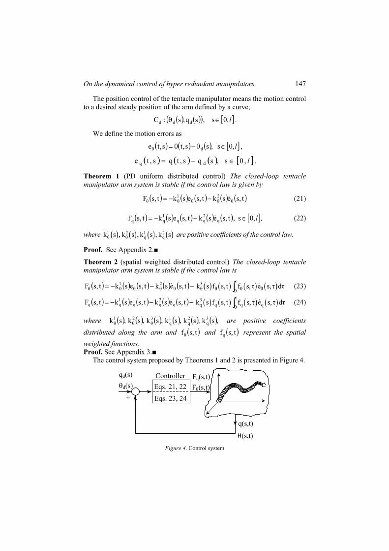
On the dynamical control of hyper redundant manipulators 147
The position control of the tentacle manipulator means the motion control to a desired steady position of the arm defined by a curve,
( ) ( )( ) [ ]l,0s,sq,s:C ddd ∈θ .
We define the motion errors as
( ) ( ) ( ) [ ]l,0s,ss,ts,te d ∈θ−θ=θ ,
( ) ( ) ( ) [ ]l,0s,sqs,tqs,te dq ∈−= .
Theorem 1 (PD uniform distributed control) The closed-loop tentacle manipulator arm system is stable if the control law is given by
( ) ( ) ( ) ( ) ( )t,seskt,seskt,sF 21θθθθθ −−= (21)
( ) ( ) ( ) ( ) ( ) [ ]l,0s,t,seskt,seskt,sF q2qq
1qq ∈−−= , (22)
where ( ) ( ) ( ) ( )1 2 1 2q qk s , k s , k s , k sθ θ are positive coefficients of the control law.
Proof.. See Appendix 2.
Theorem 2 (spatial weighted distributed control) The closed-loop tentacle manipulator arm system is stable if the control law is
( ) ( ) ( ) ( ) ( )−−−= θθθθθ t,seskt,seskt,sF 21 ( ) ( ) ( ) ( )t3θ θ θ θ0
k s f s, t f s,τ e s,τ dτ∫ (23)
( ) ( ) ( ) ( ) ( )−−−= t,seskt,seskt,sF q2qq
1qq ( ) ( ) ( ) ( )t3
q q q q0k s f s, t f s,τ e s,τ dτ∫ (24)
where ( ) ( ) ( ) ( ) ( ) ( ),sk,sk,sk,sk,sk,sk 3q
2q
1q
321θθθ are positive coefficients
distributed along the arm and ( )t,sfθ and ( )t,sfq represent the spatial weighted functions. Proof. See Appendix 3. The control system proposed by Theorems 1 and 2 is presented in Figure 4.
_ +
Fq(s,t)Fθ(s,t)Eqs. 21, 22
Eqs. 23, 24
Controllerqd(s) θd(s)
q(s,t)
θ(s,t) Figure 4. Control system

ADVANCES IN AUTOMATIC CONTROL 148
Equations (21), (22) and (23), (24) define a generalized PD controller with good performances of the position control for an ideal tentacle model without friction and internal damping and for a control criterion defined by a steady desired position.
5. Discussion a. The stability proofs are independent of the system dynamics and thus the problems associated with model-based controllers (Ivanescu, 1984; Ivanescu and Stoian 1995; Ge et al., 1996) are avoided. Also, the controllers (21), (22) and (23), (24), respectively, are independent of the system parameters and thus possess stability robustness to system parameter uncertainties. b. The infinite dimensionality of the system determines difficulties in the selection of the control parameters .k,k,k,k 2
q1q
21θθ Of course, the closed-
loop system stability requires only as ,0k1 >θ ,0k 2 >θ ,0k1q > 0k 2
q > but a practical experiment or simulation imposes a procedure in order to reach an adequate performance. Certainly, this parameter selection had to be associated with dynamic model of the system. Difficulty of the problem determines methods, rather heuristic, to evaluate the control coefficients. c. We will suggest an approximate method for evaluating the control parameters. We assume that: A1. The arm motion is a “small” motion that verifies the condition:
( ) ( ) ,t,sqt,sq δ<′′−′ [ ],s,0s,s ∈′′′ [ ]ft,0t∈ , (25)
where δ is a positive constant, sufficiently small. A2. A sequential spatial control is assumed, the elements of the arm achieve the desired position step by step: the first element achieves the desired position, then the second, and so on. The control system (21), (22), by the conditions A1, A2, can be approximated in the error space by the equation
,0ehgekeke iii2
1i
i2
2i
i =∆
+∆ρ
+∆ρ
+ N,...,2,1i = , (26)
where ( )idii qhh = represents the nonlinear term determined in the error
space by the gravitational component and 2i
1i k,k corresponds to 2
q1q ii
k,k or
,k,k 21ii θθ in the q -plane or θ -plane, respectively. (The procedure is
presented in the section 6). Equation (26) can be rewritten in the classic terms of the damping ratio
iζ and the natural frequency ,inω

On the dynamical control of hyper redundant manipulators 149
i i
2 *i i n i i i ine 2 e e h e 0+ ζ ω + ω + = , (27)
where
i
11 2i
n 2
k ω = ρ∆
(28)
( )2
11i
2
2i
i
k2
k
∆ρ=ζ (29)
i*i hgh
∆= . (30)
For this model, we suggest a method based by the sliding mode control in which the trajectory is forced along the switching line, directly to the origin, by the control of damping ratio iζ (Figure 5).
ei
-m
ei . O
DSMC
DSMC
Figure 5. Direct Sliding Mode Control
This special control is named DSMC (Direct Sliding Mode Control) and was introduced for linear systems. Ivanescu and Stoian (1995) presented an extension for nonlinear systems. The DSMC control can be obtained if the damping ratio iζ verifies the conditions (see the following Section):
2n
*i2
ii
h1ω
+>ζ (31)
2n
*i i
h ω−> . (32)
The increasing of iζ determines an over damped motion but we appreciate that this control ensures a good robustness of the global system. d. This parameter selection is based by the approximate system but it can be used in order to establish the main domains of the control coefficients.

ADVANCES IN AUTOMATIC CONTROL 150
Simulation examples presented in the following Section will confirm this procedure. e. The functions ( ) ( )t,sf,t,sf qθ can be introduced in order to achieve good performances when the desired trajectory has a "non-smooth form", with corners and group forms. We can use as fθ, fq the functions of the distance between the real position and the corner points (or terminal points) of the desired trajectory.
6. Simulations In this section, some numerical simulations are carried out as 3D and 2D tentacle manipulators. Test 1. We consider a spatial tentacle manipulator that operates in OXYZ space. The mechanical parameters are: linear density ρ=2.2 kg/m and the length of the arm l = 0.6 m. The initial position of the arm is assumed to be horizontal (OY-axis),
( ) ( ) [ ]6.0,0s;00,sq;00,s ∈==θ , (33)
and the desired position is represented by a curve C1 in OXYZ frame that is defined in terms of motion parameters as
( ) ( ) s10
sq;s12
s:1C ddπ
=π
=θ . (34)
The control law is chosen as (21), (22) where the proportional and derivative coefficients are selected as
( ) ( )( ) ( )
1 1
2 2
12.5
1.58 .q
q
k s k s
k s k sθ
θ
= =
= = (35)
(The selection of coefficients will be explained in the following Test). To solve the integral-differential system (A.1.9), (A.1.10) with the control law (21), (22), (27) we used a discretization of the s-space, with an increment ∆ = 0.1 m,
si = i⋅∆ , i = 1,2, …, 6, and a MATLAB system is used for simulation. The error for the global system is defined as
( ) ( ) ( )( ) ( ) ( )( )( )∫ θ−θ+−=l
0
2d
2d dsst,ssqt,sqte (36)
( ) ( ) ( )∫
∂θ∂
+∂∂
=l
0
dst,st
t,stqte . (37)

On the dynamical control of hyper redundant manipulators 151
The result of simulation is presented in Figure 6. We selected only most significant five intermediary positions of the motion and the phase portrait has the form presented in Figure 7. We see the stability of motion and error convergence to zero.
-12 -10 -8 -6 -4 -2 00
50
100
150
200
250Phase Portrait
error
d(er
ror)/
dt
Figure 6. 3D motion simulation Figure 7. 3D phase portrait
Test 2. A better understanding of the control can be obtained for 2D tentacle arm. We analyze now the case of a planar tentacle model in OXZ plane. The dynamic model is obtained from the equation (A1.9), (A1.10) for ,0=θ
( ) ( ) ( )s s
2
0 0s
q0
q cos q q q sin q q q q sin q q ds ds
g cosq ds F .
′ ′ ′′ ′ ′′ ′ ′ ′′ ′′ ′ ′ ′′ ρ − + − − − +
′ ′+ρ =
∫∫
∫ (38)
The control law is reduced to the form
( ) ( ) ( )( ) ( )t,sqksqt,sqkt,sF 2qd
1qq −−−= . (39)
A spatial discretization ,is ∆= i = 1, 2, …, 6, is introduced. The system (38), (39) can be rewritten in the error space by using the constraint A1 (Section 5) as
( ) 0eqhgekekem
1iidii
1qi
2q
m
1ii
2ii
=∑ρ+++∑∆ρ==
, (40)
where ( ) ( ) ( ) ( )∆−∆=∆= iqt,iqt,iete di (41)
( )∆=
=
∂∂
=
isqq
didq
Hqh (42)

ADVANCES IN AUTOMATIC CONTROL 152
and ( )qHH = is determined by the gravitational component
( ) qcosqH = . (43)
A sequential spatial control strategy (constraint A2 – Section 5) determines a decomposition of the global motion. For the first element, m = 1,
0eghekeke 1111q1
2q1
211
=ρ+++∆ρ , (44)
the control law determines
( ) 0telim 1t=
∞→. (45)
Then, for the second element, m = 2,
0eghekeke 2221q2
2q2
222
=ρ+++∆ρ , (46) we obtain ( ) 0telim 2t
=∞→
. (47)
We repeat the procedure for each element, m = 3, 4, … . In this case, we can use for each element the dynamic model
,0eqsingee2e idi2ninii iii
=⋅∆
−ω+ωζ+ i = 1, 2, …, 6. (48)
The DSMC control (Figure 5) imposes the condition
mee
i
i −= . (49)
The condition for convergence of the motion to zero, on the switching line (49), can readily be found as
2n
d2i
i
iqsing
1ω∆
⋅−>ζ (50)
2nd ii
qsingω<
∆. (51)
For the simulation test we choose the initial position of the arm as the vertical line (OZ-axis)
( ) [ ]6.0,0s,2
0,sq:2D ∈π
= , (52)
and the desired position is a semicircle, that is approximated by

On the dynamical control of hyper redundant manipulators 153
( ) 6,...,2,1i,6
s3
sq:2C iid =π
−π
= . (53)
We choose an uniform natural frequency ,24in =ω i=1, 2, …, 6, and for
verifying the conditions (50), (51), (53) we select
,5.1i =ζ i=1, 2, …, 6. (54)
From (28), (29) we obtain the control coefficients
,5.12k1i = ,58.1k2
i = i=1,2,…,6. (55)
The results of the simulations are presented in Figure 8 and the phase portrait is plotted in Figure 9.
0 0.01 0.02 0.03 0.04 0.05 0.06-3.5
-3
-2.5
-2
-1.5
-1
-0.5
0
0.5Phase Portrait
error
d(er
ror)
/dt
Figure 8. 2D phase portrait Figure 9. 2D motion simulation
7. Conclusions The paper treats the control problem of a tentacle manipulator. In order to avoid the difficulties generated by the complexity of the nonlinear integral-differential equations that define the dynamic model of this system, the control problem is avoided by using a very basic energy relationship of this dynamic model. The energy relationships of a tentacle manipulator are inferred. An energy-based control law is introduced by using only the relations that determine the energy stored in the system. Two controllers are proposed that generate the PD control laws and a procedure of control coefficient selection is discussed. In Appendix 1 is obtained the dynamic model of a spatial tentacle arm that allows for the checking of the control laws. Numerical simulations for spatial and planar tentacle models illustrate the efficiency of the method.

ADVANCES IN AUTOMATIC CONTROL 154
Appendix 1 We will consider a spatial tentacle model, an ideal system, neglecting friction and structural damping. We assume a uniformly distributed mass with a linear density ρ [kg/m]. We will consider a non-extensible arm with a constant length l (Figure 2a, 2b). We will use the notations: ( ) [ ] [ ]ft,0t,,0s,t,sqq ∈∈= l ,
( ) [ ] [ ]ft,0t,,0s,t,s ∈∈θ=θ l ,
( ) [ ] [ ]ft,0t,s,0s,t,sqq ∈∈′′=′ ,
( ) [ ] [ ]ft,0t,,0s,t
t,sqq ∈∈∂
∂= l ,
( ) [ ] [ ]ft,0t,s,0s,t
t,sqq ∈∈′∂′∂
=′ ,
( ) [ ] [ ]f2
2
t,0t,s,0s,t
t,sqq ∈∈′∂
′∂=′ ,
( ) [ ] [ ]f2
2
t,0t,s,0s,t
t,sqq ∈∈′′∂
′′∂=′′ ,
. . . . . . . . . . . . . . . . . . . . . . . . . . . . .. . ,
( ) [ ] [ ]fqq t,0t,,0s,t,sFF ∈∈= l ,
. . . . . . . . . . . . . . . . . . . . . . . . . . . . . . . .
The position of a point P is
s
0s
0s
0
x = cosq sinθ ds
y = cosq cosθ ds
z = sinq ds
′ ′ ′
′ ′ ′
′ ′
∫
∫
∫
(A.1.1)
and the velocity components are
( )( )
sx 0
sy 0
sz 0
v = -q sinq sinθ + θ cosq cosθ ds
v = -q sinq cosθ -θ cosq sinθ ds
v = qcosq ds .
′ ′ ′ ′ ′ ′ ′
′ ′ ′ ′ ′ ′ ′
′ ′
∫
∫
∫
(A.1.2)
For an element dm, kinetic and potential energy will be

On the dynamical control of hyper redundant manipulators 155
2k vdm
21dW ⋅= (A.1.3)
zgdmdWp ⋅⋅= , (A.1.4)
where dm = ρds. (A.1.5) From (A.1.2)-(A.1.5) we obtain,
( )
( )
2s
k0 0
2 2s s
0 0
1W qsinq sin cosq cos ds2
q sinq cos cosq sin ds q cosq ds ds
l ′ ′ ′ ′ ′ ′= ρ − θ + θ θ + ′ ′ ′ ′ ′ ′ ′ ′ ′ ′+ − θ − θ θ +
∫ ∫
∫ ∫
(A.1.6)
∫ ∫ ′′ρ=l
0
s
0p dssdqsingW . (A.1.7)
The dynamic model is obtained by using Lagrange equations of motion
Fq
Wq
Wq
Wdtd pkk =
∂
∂+
∂∂
−
∂∂ , (A.1.8)
where qW∂∂
denotes a functional partial (variational) Gateaux derivative
(Wang, 1965) that is defined as the variation of the functional W with respect to the function q at a point s∈[0, l]. From (A.1.6), (A.1.7) it results,
( )( )(∫ ∫ −′′′+′′−′′′′′ρs
0
s
0
qcosqcosqqcosqsinqsinq ( ) +θ′−θ ′′′′′θ′ sinqsinqcos
( )( )+′′′−θ ′′−θ′′′′′+ qcosqsincosqsinqcosq 2 ( ) −θ ′′−θ′′′′θ′ cosqsinqcos2
( )) +′′′′−′′′′′− sdsdqqsinqq ∫ =′′ρs
0qFsdqcosg (A.1.9)
( )(∫ ∫ +θ′−θ ′′′′′′ρs
0
s
0
sinqcosqsinq ( ) −θ′−θ ′′′′′θ′ cosqcosqcos
( )+θ′−θ ′′′′′′− sinqcosqcosq 2 ( ) −θ′−θ ′′′′′θ′ sinqcosqcos ( )) θ=′′′θ′−θ ′′′′′′θ′− Fsdsdcosqcosqsinq . (A.1.10)

ADVANCES IN AUTOMATIC CONTROL 156
Appendix 2 We consider the following Lyapunov function (Ivanescu, 1984)
( ) ( ) ( ) ( ) ( ) ( ) ( )( )dst,seskt,sesk21tWtWtV
0
2q
1q
21pk ∫ +++= θθ
l
. (A.2.1)
V(t) is positive definite because the terms that represent the energy WK and WP are always
WK(t) ≥ 0, WP(t) ≥ 0 .
From (17) we obtain (for a steady desired position),
( ) ( ) ( ) ( ) ( )( ( ) ( ) ( ) ( ) ( ) ( )1 1q q q q q
0
V t F s,t e s,t F s,t e s,t k s e s,t e s,t k s e s,t e s,tl
θ θ θ θ θ= + + +∫ .
(A.2.2)
If we use the control law defined by the relations (21) and (22), we will have
( ) ( ) ( )( ) ( ) ( )( )( )∫ +−= θθ
l
0
2q
1q
21 dst,seskt,sesktV (A.2.3)
( ) 0tV ≤ . (Q.E.D)
Appendix 3 We extend the Lyapunov function (A.2.1) as
( ) ( ) ( ) ( ) ( ) ( ) ( )( 1 2 1 2k p q q
0
1V t W t W t k s e s,t k s,t e s,t2
l
θ θ= + + + +∫
( ) ( ) ( ) +
ττ⋅τ+ ∫ θθθ
2t
0
3 d,sf,sesk ( ) ( ) ( ) dsd,sf,sesk2t
0qq
3q
ττ⋅τ∫ .(A.3.1)
In this case,
( ) ( ) ( ) ( ) ( )(∫ ++= θθ
l
0qq t,set,sFt,set,sFtV
+ ( ) ( ) ( ) ( ) ( ) ( ) ++θθθ t,set,seskt,set,sesk qq1q
1
( ) ( ) ( ) ( ) ( ) +τττ+ ∫ θθθθθ
t
0
3 d,sf,set,sft,sesk

On the dynamical control of hyper redundant manipulators 157
+ ( ) ( ) ( ) ( ) ( ) dsd,sf,set,sft,seskt
0qqqq
3q
τττ∫ (A.3.2)
and by using the control laws (23) and (24) we obtain
( ) ( ) ( )( ) ( ) ( )( )( )∫ +θ−= θ
l
0
21q
21 dst,sqskt,ssktV (A.3.3)
( ) 0tV ≤ . (Q.E.D)
References Chirikjian, G. S. and J. W. Burdick (1990) An Obstacle Avoidance Algorithm for Hyper-
Redundant Manipulators, Proc. IEEE Int. Conf. on Robotics and Automation, Cincinatti, Ohio, May, pp. 625 – 631.
Chirikjian, G. S. and J. W. Burdick (1992). Kinematically Optimal Hyper-Redundant Manipulator Configurations, Proc. IEEE Int. Conf. on Robotics and Automation, Nice, May, pp. 415 – 420.
Chirikjian, G. S. (1993a). A General Numerical Method for Hyper-Redundant Manipulator Inverse Kinematics, Proc. IEEE Int. Conf. on Robotics and Automation, Atlanta, May, pp. 107 – 112.
Chirikjian, G. S. (1993b). A Continuum Approach to Hyper-Redundant Manipulator Dynamics, Proc. 1993 Int. Conf. on Intelligent Robots and Systems, Yokohama, Japan, July, pp. 1059-1066.
Chirikjian, G. S. and J. W. Burdick (1995). Kinematically Optimal Hyper-Redundant Manipulator Configurations, IEEE Trans. Robotics and Automation, vol. 11, no. 6, Dec., pp. 794 – 798.
Cieslak, R. and A. Moreki (1994). Technical Aspects of Design and Control of Elastic’s Manipulator of the Elephants Trunk Type, 5th World Conference on Robotics Research, Sept. 27-29, Cambridge, Massachusetts, pp. 1351-1364.
De Laurentis, K.I. (2002). Optimal Design of Shape Memory Alloy Wire Bundle Actuators, Proc. of the 2002 IEEE Int. Conf. on Robotics and Automation, Washington, May, pp. 2363-2368.
Ge, S.S., T.H. Lee and G. Zhu (1996). Energy-Based Robust Controller Design for Multi-Link Flexible Robots, Mechatronics, vol. 6, no. 7, pp. 779-798.
Gravagne, I.D. and I. D. Walker (2000). On the kinematics of Remotely - Actuated Continuum Robots, Proc. 2000 IEEE Int. Conf. on Robotics and Automation, San Francisco, April, pp. 2544-2550.
Gravagne, I.D. and I. D. Walker (2001). Manipulability, Force, Compliance Analysis for Planar Continuum Manipulators, Proc. IEEE / RSI International Conference o Intelligent Robots and Systems, pp. 1846-1867.
Hale, J.K. and J.P. Lasalle (1967). Differential Equations and Dynamical Systems, Academic Press.

ADVANCES IN AUTOMATIC CONTROL 158
Hemami, A. (1984). Design of Light Weight Flexible Robot Arm, Robots 8 Conference Proceedings, Detroit, USA, June 4-7, pp. 1623-1640.
Ivanescu, M. (1984). Dynamic Control for a Tentacle Manipulator, Proc. Int. Conf. on Robotics and Factories of the Future, Charlotte, pp. 315-327.
Ivanescu, M. and V. Stoian (1995). A Variable Structure Controller for a Tentacle Manipulator, Proc. IEEE Int. Conf. on Robotics and Automation, Nagoya, May 21-27, pp. 3155-3160.
Mishkin, E. and L. Braun Jr. (1961). Adaptive Control Systems, New York, McGraw Hill.
Mochiyama, H., E. Shimeura and H. Kobayashi (1998). Direct Kinematics of Manipulators with Hyper Degrees of Freedom and Serret-Frenet Formula, Proc. 1998 IEEE Int. Conf. on Robotics and Automation, Leuven, Belgium, May, pp. 1653-1658.
Mochiyama, H. and H. Kobayashi (1999). The Shape Jacobian of a Manipulator with HyperDegrees of Freedom, Proc. 1999 IEEE Int. Conf. on Robotics and Automation, Detroit, May, pp. 2837-2842.
Robinson, G. and J.B.C. Davies (1999). Continuum Robots – A State of the Art, Proc. 1999 IEEE Int. Conf. on Robotics and Automation, Detroit, Michigan, May, pp. 2849-2854.
Shigoma, K. B. (1996). Robot Grasp Synthesis Algorithms: A Survey, The International Journal of Robotics Research, vol. 15, no. 3, pp. 230-266.
Suzumori, K., S. Iikurav and H. Tanaka (1991). Development of Flexible Micro-Actuator and its Application to Robot Mechanisms, IEEE Conference on Robotics and Automation, Sacramento CA, April, pp 1564-1573.
Wang, P.K.C. (1965). Control of Distributed Parameter Systems, in Advance in Control Systems, by C.T. Leondes, Academic Press.
Wang, L.-X. (1999). Analysis and Design of Hierarchical Fuzzy Systems, IEEE Trans. on Fuzzy Systems, vol. 7, No. 5, Oct., pp. 617-624.
Wang, Z.P., S.S. Ge and T.H. Lee (2001). Non-Model-Based Robust Control of Multi-Link Smart Materials Robots, Asian Conference on Robotics and its Applications, 6-8 June, Singapore, pp. 268-273.

ROBOTS FOR HUMANITARIAN DEMINING
P. Kopacek Institute of Handling Devices and Robotics, Vienna University of Technology Favoritenstr. 9–11, A–1040 Vienna, Austria [email protected]
Abstract “Humanitarian demining”, is growing up dramatically in the last decade. Here a new idea – application of a very well known tool from production automation “advanced robots” - will be presented. These robots of the new generation offer possibilities to solve this task in a very efficient way. Finally “Humanitarian Demining Multi Agent Systems – HDMAS” an autonomous, intelligent robot swarm for cleaning minefields in the future is discussed.
Keywords: landmines, demining, robots, MAS, robot swarms
1. Introduction According to current estimates, more than 100.000.000 anti-personnel and other landmines have been laid in different parts of the world. A similar number exists in stockpiles and it is estimated that about two million new ones are being laid each year. According to recent estimates, mines and other unexploded ordnance are killing between 500 and 800 people, and maiming 2.000 others per month (Red Cross, 1995), mainly innocent civilians who had little or no part in the conflicts for which the mines were laid. Anti-personnel mines are usually designed not to kill, but to inflict horrible injuries instead (McGrath, 1994). However, many victims eventually die of their injuries, and suffer a long and agonizing death, often with little medical attention. Some countries have banned the use of landmines and others are supportive of a complete ban. However, their low cost ($1- $30) and the large numbers in existing stockpiles make them an attractive weapon for insurgency groups which operate in may countries with internal conflicts – the most common cause of wars today. They are used for self-defense

ADVANCES IN AUTOMATIC CONTROL 160
by villages and groups of people traveling in many districts where civil law and order provide little effective protection. Many countries retain massive landmine barriers on their borders or near military installations. Some of the most severe landmine problems exist in Egypt, Angola, Afghanistan, Rwanda, Bosnia, Cambodia, Laos, Kuwait, Iraq, Chechnya, Kashmir, Somalia, Sudan, Ethiopia, Mozambique and the Falkland Islands.
2. Landmines Landmines are usually very simple devices which are readily manufactured anywhere. There are two basic types of mines: anti-vehicle or anti-tank (AT) mines and anti-personnel (AP) mines. AT mines are comparatively large (0.8 – 4 kg explosive), usually laid in unsealed roads or potholes, and detonate which a vehicle drives over one. They are typically activated by force (>100 kg), magnetic influence or remote control. AP mines are much smaller (80-250g explosive, 7-15cm diameter) and are usually activated by force (3-20kg) or tripwires. There are currently over 700 known types with different designs and actuation mechanisms. We have two main categories of AP mines. A blast mine is usually small and detonates which a person steps on it: the shoe and foot is destroyed and fragments of bone blast upwards destroying the leg. When a fragmentation mine explodes, metal fragments are propelled out at high velocity causing death or serious injuries to a radius of 30 or even 100 meters, and penetrating up to several millimeters of steel if close enough. Simple fragmentation mines are installed on knee high wooden posts and activated by tripwires (stake mines). Another common type of fragmentation mine (a bounding mine) is buried in the ground. When activated, it jumps up before exploding. Mines of one type have often been laid in combination with another type to make clearance more difficult: stake mines with tripwires may have buried blast mines placed around them.
3. Demining; state of the art First you have to find the mines and then you must destroy. Used methods for identifying mines today are:
- Manually: by humans – deminers – equipped with e.g. metal detectors.
- Dogs: using dogs that sniff the explosive contents of the mines, has significant limitations and cannot be regarded to as general-purpose solution.
- High-tech methods for mine detection: radar, infrared, magnetic tools,

Robots for humanitarian demining 161
touching sensors (piezo resistive sensor) …. Also GPS is used for finding the place again where a mine lies, and for the navigation of the robots.
Today used methods for destroying and removal are: brutal force methods include ploughs, rakes, heavy rolls, flails mounted on tanks. The problems with these methods are that.
- Ploughs only can by used to clear roads for military use. Mines are only pushed to the side of the road. Some ploughs also attempt to sieve the mines from the displaced soil.
- Flails are mechanical devices, which repeatedly beat the ground, typically with lengths of chain. These chains are attached to a rotating drum and their impact on the ground causes the mines to explode, but this can cause severe damage to cultivable land.
- Rollers generally consist of a number of heavy circular discs, which are rolled along the ground in order to cause the explosion of any mines.
Before demining can start, surveys are needed to produce detailed maps of minefields to be cleared. The survey team may use specially trained dogs to narrow down the limits of a mined area, and normally verifies a one or two meter wide “safe lane” around each minefield to define the minefield which may be surrounded with unknown land or other minefields. Typical minefields are 100-200m across and 0.1-10ha in area. Hand-prodding is today the most reliable method of mine clearing, but it is a very slow, and extremely dangerous. People performing this type of clearing can normally only perform this task for twenty minutes before requiring a rest. This method clears one square meter of land in approximately 4 minutes. The tools of a deminer are:
1. A whisker wire which is gently swung or lifted to check for tripwires.
2. A metal detector which is swung from side to side to check for metal objects.
3. A prodder (typically a bayonet, screw driver or knife) which is used to probe the ground at an angle of about 30 degrees to the horizontal and to excavate earth from around a suspect object. Usually a prodder is used to investigate a suspect metal object. However, which dealing with minimum metal mines or large numbers of metal fragments, the entire area has to be prodded by hand.
The UN estimates the cost of removing a single mine at 300 to 1000 $. The primary factor is the local cost of labor. So in low labor-cost countries such as (Cambodia, Afghanistan, or Africa) US$ 100 per month is a high rate pay for manual work, even with the obvious risks. In contrast, the labor cost for de-mining in the former Yugoslavia may be twenty times higher.

ADVANCES IN AUTOMATIC CONTROL 162
Thinking about the number of mines is rather pointless which estimates range from a few million word-wide (including national borders) to 150 million. It is much more sensible to think in terms of the areas of land which are:
a) known to be affected by mines, and are important to local or displaced population:
homes, food producing land, roads, infrastructure (roads, canals, power lines, water supplies etc.);
b) believed to be affected by mines; c) known or believed to be affected by mines, but land is of no
immediate importance. The standard which is required for humanitarian demining is a guaranteed 99.6% clearance. Therefore the remaining risk to be injured or killed by a mine is 0.4%. Mechanical mine clearance means either actuating the mine, or removing it for later destruction. For actuating ploughs are pushed by a tank or an armored bulldozer. There is a bulldozer with a rotating cylinder in front, digging up to 50cm into the ground. The vehicle has been tested in Mozambique. Although it did not reach the 99.6% UN requirements, it removed 25.000 mines in a six-month campaign. Another demining vehicle uses the same principle, with closer teeth. It is based on a Leopard 1 main battle tank chassis to which a rotating roller is added. The tank can be remote controlled from 500m away. In normal terrain this vehicle should clear up to 20.000 square meters per hour with total safety for the mine-clearing team. The disadvantage is that mines includes a lot of chemicals which when they detonate are put into the ground which is later used for food producing.
4. Robots for demining
4.1. State of the art Several projects have proposed the use of autonomous robots to search for antipersonnel mines. The sensor problem is nearly solved now and it will take only little time until a combination of sensors will be available and sufficiently tested in order to give full confidence that all the mines have been discovered. There may be false alarms, but no mine must be left. Once the location of a mine is known, several manual techniques are easily applied to neutralize it. A robot can also be developed to do this easy job, which is simply to go to a precise spot, avoiding obstacles and other mine locations. Then it should deposit a shaped charge or some chemical to destroy the mine. The necessary features of a demining robot are:
- Ability to distinguish mines from false alarms like soil clumps, rocks, bottles and tree roots.

Robots for humanitarian demining 163
- Operation in a variety of soil types, moisture contents and compaction states.
- Ability to detect both types or in fact variety of different mine types and sizes.
- Operation in vegetated ground cover. - Costs may be lower then 10.000 US$ including the sensors.
Today there are some appropriate, reasonable cheap sensors available or in development based on optical technologies, acoustic and seismic detection, radio frequency resonance absorption spectroscopy, trace explosion detection. Worldwide approximately 100 companies or research institutes offers intelligent, mobile platforms but the price is too high according to the small lot sizes in production. It’s only a question of time until this problem is solved. Random navigation for covering the field and searching for mines has been proposed. Even with improved algorithms applied to a group of robots, it is difficult to accept ignoring a small proportion of uncovered areas. Systematic navigation is theoretically easy with a global positioning system (GPS), but the resolution must be better than the size of the detector, in order to be sure to cover all the area. A robot has been designed as a light-weight autonomous robot to search for antipersonnel mines. The pressure force on the ground, 5kg, is not intended to trigger the mines. The sensor head oscillates under the alternating movement of the wheels, in order to scan a width of about 1.2 m. the project is suspended until an adequate sensor, weighing less than 4kg, can be installed inside the head. Research groups experienced with walking robots try to suggest the use of their devices for this application. Snake robots are more attractive, since they should be able to crawl close to the ground inside dense vegetation. Their design is, however, quite challenging. The advantages of robots for demining are
- Minefields are dangerous to humans; a robotic solution allows human operators to be physically removed from the hazardous area.
- Robots can be designed not to detonate mines. - The use of multiple, inexpensive robotized search elements minimizes
damage due to unexpected exploding mines, and allows the rest of the mission to be carried on by the remaining elements.
- Teams of robots can be connected so that one team is for searching and one for destroying or displacement.
This means that many robots are searching and a few or only one robot is destroying or displacing the mines. But there are also disadvantages of using robots:
- it is very difficult for robots to operate in different frequently rough terrain;

ADVANCES IN AUTOMATIC CONTROL 164
- they are still expensive; - you need special qualified operators.
4.2. Multi Agent Systems - MAS
A MAS consists of a number of intelligent, co-operative and communicative hardware agents – mobile robots – getting a common task. Because of the intelligence they are able to divide the task in subtasks as long as at least one agent is able to fulfill one subtask. Repeating this procedure yields the solution of the common task. Newest research goes in the direction of MMAS - Multiple Multi Agent Systems – different MAS are involved for the solution of a complex task. A MAS get a whole task. The host computer divides the whole task in a number of different subtasks as long as a distinct subtask can be carried out by at least one agent. The agents will fulfill their subtasks in a cooperative way until the whole task is solved. Such a global task could be: assemble a car. The agents – mobile, intelligent assembly robots – have to create subtasks (e.g. assembling of wheels, windows, brakes,......) in an optimal way (equal distribution of the workload of the agents) and distribute to the agents. The main hurdles for MAS-research are the complexity of the whole system. This complexity is dramatically increasing by adding new agents. Therefore the interaction, communication, coordination of the tasks between agents, and control are the topics for the development of a Multi Agent System ( MAS ). For heterogeneous robots it is difficult to implement the communication, because each robot has its own kinematical structure, programming language etc.. Furthermore the range of frequencies used for communication and the capability of RF modules is limited. It is necessary to develop standardized communication protocols and methods, which should be one of the works for the next years. Fig.1a. shows the present situation of the communication between the host and the agents. For the future the agents should also communicate with the host and also with the other agents as shown in Fig. 1b and Fig.1c. The characteristics of MAS are:
• each agent has incomplete information or capabilities for solving the problem and, thus, has a limited viewpoint;
• there is no system global control; • data are decentralized; • computation is asynchronous.
In scientific papers one uses various approaches and denotations to subdivide control strategies for autonomous mobile robots in different types. There are two fundamental describing ideas: the functional and the behavior based approach.

Robots for humanitarian demining 165
H
A1
A2
An
a. Communication only between host and agents
H A2
A1
An
b. Partial communication between host and agents as well as between the agents
H
An
A1
A2
c. Full communication between host and agents as well as between the agents
Figure 1. Different types of MAS H : Host computer; A1, A2,.....,An : Agents;
________: full communication; ------------ : partial communication
4.3. Robot Swarms – MAS - for demining Robot swarms improve the capacity of robotic applications in different areas where robots are already used today. Robot swarms are similar to – or a synonym for - ‘Multi Agent Systems – MAS’. These systems are very well known in software engineering – “software agents” - since more than twenty years. In the last years there are more and more works related to “hardware agents” like robots forming “robot swarms”. Applying robots for demining there are two possibilities:
a. using mobile, intelligent multipurpose robots equipped with devices for mine detection, mine removing as well as mine transportation;
b. using three different swarms of single-purpose robots equipped either with detection devices or removing devices or transportation facilities.
Our approach is the second one – three different swarms in the minefield. The detection robots scan the field for possible mines. If a metallic part –

ADVANCES IN AUTOMATIC CONTROL 166
probably a landmine is detected one of the removal robots close to this site removes the mine and takes it over to a transportation robot with free capabilities. This robot transports the mine to a collection area out of the minefield. The whole process is fully autonomous. Operators are only needed for monitoring and of course maintenance. To achieve this goal the robots must have a high level of intelligence and must be able to communicate among themselves. Since the power supply of mobile robots is very limited there is also need for docking stations. The host computer in Fig. 2 is necessary to solve the path planning problem in a dynamic environment. Each robot represents for all other robots a dynamic obstacle which has to be avoided. The host computer controls the movements of all robots by means of wireless communication. But soon such a host computer will be obsolete (Fig.1c). Software implemented in the onboard computer of each robot will take over this task.
Figure 2. Humanitarian Demining Robot Swarms [Kopacek, 2002b]
Using different single purpose robots for the different tasks reduces the weight of the robots. Therefore it is much easier to design robots which are lightweight enough not to cause an explosion while crossing over a mine field. As mentioned before the use of modular robots is perfect for the design of task-specific demining robots because of the similarities between the tasks. [Shivarov, 2001] Since the complexity of a system raises the susceptibility to trouble exponential it is always better to keep devices as simple as possible and therefore to use simpler robots. Using smaller robots extends the operational time before re-fuelling or re-charging is necessary or at least prevents the use of bulky and heavy batteries or tanks. On the other side the second possibility requires an increased effort in communication between the robots in the swarm. If every robot is able to perform the whole demining process by itself the communication is reduced

Robots for humanitarian demining 167
more or less to get each other out of the way and ensure to cover all the area. However the task-specific robots have to exchange a lot more of data. The detection robots must work together since they are equipped with different detection technologies. When they have found a mine they must signal it to the removal robots and they have to inform after done work the transportation robots.
4.3.1. Detection robots
The robots for the detection of landmines are probably the most simplest of the three types. The basic composition of modules common for all three types has to be upgraded only with the detection system. There are several detection technologies in use respectively under development, none of them able to detect a mine alone by itself. The solution is to use two or more of these different sensors simultaneously. The first logical step would be to attach different sensors on one robot. Since there are weight limits, and limits in the amount of available energy, this is probably not the best solution. Some of these technologies need strong power sources and some of them are relatively heavy constructed. These facts will not help to keep the weight of the robot low, so using for each type of sensor a single robot seems to be the better solution. The detection robots should communicate with each other, change data and coordinate their work. If one robot with one distinct detection technology has found a possible target, the area should be verified by all other detection technologies before any further action is started. Therefore the different technologies must be compatible to allow coordination. At least the data from the sensors should be assessed by the same software. Combining results from different mine detection technologies is not easy and demands special strategies. These so-called sensor fusion technologies are not only of concern for mine detection. Another important point is the power supply of the detection swarm. One possibility is to equip detection robots with an autonomous power source. But this could complicate the recharging of the system. There would be need for extra docking stations and at the worst for each detection technology a different docking station. This cooperation during the development and design process of the modular robot system and landmine detection sensors is of greater concern than only for an appropriate modular interface. Some of these sensor systems are extremely sensible and may drop in performance in presence of distinct materials. Using these materials for parts of the robot system which has to carry the sensor technology has to be avoided. And many of the sensor techniques work by using radiation in some range of the electromagnetic spectrum. It has to be guaranteed that systems of the robot do not jam the sensor technology or the other way round.

ADVANCES IN AUTOMATIC CONTROL 168
4.3.2. Removal robots
The removal of landmines is probably the heaviest work during the whole de-mining process. This is clearly a matter of the type of soil in which the mines are buried. But generally this task needs the highest forces and therefore the system has to be more stiff and heavy constructed. The removal robots have also the most complex part to fulfill. While the detection robots only transport the detection technology and the transportation robots have to accomplish an advanced pick and place task, the removal robots have to, in case of buried mines, dig out a highly sensitive device, which must be handled extremely carefully, but at the same time applying relatively high forces to penetrate the soil. In addition the excavation of a mine is every time a different procedure. The main parameters which differ for each buried mine are the type and shape of the mine, the position relative to the surface and the type of soil in which the mine is buried. Since the excavation is a complex task a dexterous robot arm with a high number of degrees of freedom is likely to be used. For the mine removal various end-effectors may be necessary. The robot arm can be equipped with a variety of standard tools which are similar to tools used for manual excavation. All forms of shovels are doubtless of interest to remove foremost close grained material. Grippers may used to sweep stones or other bigger obstacles. These tools are commercially available and well proven. Up to the present the most removal work performed at hazardous materials was executed teleported. For that the aid of sensors is mainly limited to force and torque sensors which ensure not to apply too high forces to the sensible object. But the whole process is controlled by an operator using video cameras to lead the tools. Using a robot for autonomous removal of landmines presupposes the usage of sensors to compensate the teleoperator. Two broad classes of sensing technologies support earthmoving automation. One class allows determining the state of the robot itself, the other class concerns perception of the environment around the earthmover. Local state is achieved by measuring displacements at the robots various joints. If the actuators are hydraulic cylinders the use of position transducers would be a good choice. An alternative is to use joint resolvers, like potentiometers, directly at rotary joints. Another form of state estimation is to locate the robot arm with respect to some fixed coordinate frame. Many sensing modalities have been used including, GPS, inertial sensors and reflecting beacons. Successful estimation schemes combine several of these techniques.
4.3.3. Transportation robots
The transportation seems to be quite simpler than the removal of a landmine. Basically the robot has to pick up the landmine, store it somewhere during the transportation and deliver it at the collection point.

Robots for humanitarian demining 169
An important decision in respect of the transportation robots is the number of mines the robots should be able to carry. Carrying only one mine would it make possible to use a rather simple robot. At the best it may possible to retrench the storing place for the landmine. The robot could pick up the mine with a gripper, lift it up somewhat above the ground and transport it to the collection area while holding it tight with the gripper. The use of a dexterous robot arm, like that one for the removal task, would be disproportionate. A simple 2 DOF lift onboard the mobile robot platform could be sufficient. On the other side the application of a transportation robot with the ability to carry more than one mine is in a manner useful too. Since transportation robots are likely to be rather slow this approach is much more timesaving. The volume of saved time depends on the amount and distribution of collection areas in proportion to the field of activity as well. But establishing lesser collection areas simplifies the further strategy for the disposal of the collected landmines. To give the robot the ability to transport more than one mine it must be equipped with some sort of storage device. One principle would be of use to make the storage device of protective material to mitigate accidentally explosions. One possibility is to use a lockable storage device. But therefore the device must be designed with regard to a maximal allowed load of explosives. An explosion inside a locked container exceeding the maximal allowed load may be worse than without any protective measures. Fragments of the blasting container could damage the robot in addition. For this reason it would be better to use a container which is opened upwards. This guarantees a way out for the pressure wave in case of an accidental explosion. An important factor for the decision of using single or multi transport robots is the density of the minefield. If there are only few landmines per surface unit the application of single-mine transportation robots is more likely. In this case the work quota of the detection robots is much higher compared to that of the removal and transportation robots. Therefore raising the working capacity of the transportation robots would not increase the overall efficiency perceptible.
4.4. Realization The features of the robot for these three tasks have to be quite different. For detection a light-weight robot only able to carry little load has to be developed. For removal the robot has to be more stiff and heavy constructed because removal requires force. The size of transportation robots depends on the number and kind of the mines to be transported. Another point of view which has to be taken into account is the time necessary for these operations. Detection is usually relatively fast and is not so time consuming than removal. According to some experiences the

ADVANCES IN AUTOMATIC CONTROL 170
removing time is 3 to 5 times more than the detection time. Transportation time is also relatively small. Therefore it could be advantageous to use three different types of robots (Fig. 2): robots for detection (D), robots for removal (R) and robots for transportation (T) of the mines. One main disadvantage of this philosophy is if a robot of the swarm D (detection) has found or detected a mine it has to send a command to the host computer or to the other robots. The host computer or the other robots have to decide which of the robots of the swarm R (removal) is in the neighborhood of this mine and not busy at that time with removal operations on another mine. If a robot of the swarm R is selected this robot gets usually wireless the position data and some other information about the place of the mine. The R robot is now moving to displace and start with the removal work. After the removal of the mine it has to place the mine on the ground in a distinct position. One of the transportation robots (T) have to pick up the mines and have to carry it to a collecting place.
4.4.1. Mobile robots
Today we are in the position to develop robots of all three types mainly using commercially available mobile platforms. As pointed out earlier it is not economically feasible to develop so-called single purpose robots for each of these three types. A good approach could be a kind of a tool kit [Shivarov, 2001] of mobile robots consisting of a mobile platform and different equipments and tools compatible in hard- and software. A good approach could be to have two platforms, one with wheels or chains and one walking platform. According to the types of mines as well as the surface of the minefield these platforms could be equipped with necessary tools in a very short time. Usually the mobile robots of both types available today are moving relatively slow. Speed for wheeled and chained robots is between 0.5 and 0.7 m/s, walking robots are usually much slower. This could be a disadvantage concerning the demining time but from the viewpoint of control and path planning it is much easier to work with such slow robots. We have in that case the usual problem of path planning of robots in a changing environment. Usually in a minefield we have fixed obstacles like trees, rocks, buildings as well as moving obstacles usually the robots of the own or other swarms.
4.4.2. Humanoid robots [Kopacek, 2003]
The main feature of a real human is the two legged movement and the two legged way of walking. In principle the stability during the walking decreases with the number of the legs. At the begin of this development there were consequently 8, 6 and 4 legged robots copied from the nature (insects, swarms,

Robots for humanitarian demining 171
…). In the future two legged robots should be responsible for human tasks like service applications, dangerous tasks, tasks on the production level, support of humans in everyday life … The main advantage of legged robots is the ability to move in a rough terrain without restrictions like wheeled and chained robots. Two legged robots could work in environments which were until now reserved only for humans. In addition to walking such robot could realize other movements like climbing, jumping, swimming, …. Walking robots are much more flexible than robots with other movement possibilities. Especially fixed and moved obstacles can be surmounted by legged robots. Two legged robots require new technologies in the field of robotics. In some cases a combination from well known methods of mechanical engineering, electrical engineering, electronics, control engineering, computer sciences, applied physics are necessary. Currently there are worldwide two categories of two legged humanoid robots available:
• “Professional” humanoid robots. • “Research” humanoid robots.
The humanoid robots of the first category are mostly developed but very expensive and currently not available on the market. The robots of the second category a usually prototypes Therefore for several tasks e.g. humanitarian demining a two legged, humanoid robot should be developed. These robots could be applied for all three tasks of demining – detection, removing and transportation in the future.
5. Summary As pointed out demining is today a very time consuming, dangerous and expensive task. Automatic demining e.g. as presented in this paper by robots, is today and will be in the future a powerful tool to solve these problems. All the existing and planed robots for humanitarian demining are only able to detect the mines. Brutal force methods destroy mines without detection – but with a not reasonable probability. In a next step our robots have to be able to remove the mines from the ground. “Multi Agent Systems – MAS” [Kopacek, 2002a] are very well known in software engineering since more than 20 years. In the last years there are some works related to the application in production automation. A MAS consists of a number of intelligent, co-operative and communicative hardware agents e.g. robots getting a common task. Because of the intelligence they are able to divide the whole task in subtasks as long as at least one of the agents is able to fulfill one subtask. Repeating this procedure yields the solution of the common task. Newest

ADVANCES IN AUTOMATIC CONTROL 172
research goes in the direction of MMAS – Multiple Multi Agent Systems – different MAS are involved for the solution of a complex task. In a mid or long term perspective it might be possible to develop “Humanitarian Demining Multi Agent Systems – HDMAS ” consisting of a number of such robots or agents [3]. Robot swarms or HDMAS for demining especially with two legged (humanoid) robots are currently only a vision but will be reality in the nearest future.
References McGrath, R. (1994): Landmines, Legacy of Conflict: A Manual for Development Workers,
Oxfam, Oxford.
Red Cross (1995): Landmines must be stopped. International Committee of Red Cross, Geneva, Switzerland.
Trevelyan, J. (1997): Robots and landmines. Industrial Robot, 24 (1997), Nr.2, p.114-125
Baudoin, Y. et.al. (2000): “Humanitarian Demining: Sensory and Robotics”. Proceedings of the IMEKO World Congress 2000, Vienna, Vol. XI, p. 241 – 251.
Kopacek, P. (2000): “SWIIS – An Important Expression of IFAC’s Commitment to Social responsibility”, Preprints of the IFAC Workshop on Supplemental Ways for Improving International Stability – SWIIS 2000, May 2000, Ohrid, Macedonia.
Shivarov, N. (2001): “A tool kit for modular, intelligent, mobile robots”. PhD. Thesis, Vienna University of Technology, 2001.
Kopacek, P. (2002a): “Demining Robots – a tool for International Stability”. Proceedings of the 16th IFAC World Congress, Barcelona, July 2002.
Kopacek, P. (2002b): Robot Swarms for Demining. Proceedings of the IARP Workshop “Robots for Humanitarian Demining – HUDEM`02”, Vienna, Austria, 2002; p. 39-44.
Kopacek, P. (2003): Humanoid Robots for Demining – Vision or Reality. Proceedings of the IARP Workshop “Robots for Humanitarian Demining – HUDEM`03”, Pristina, Kosovo, 2003 (In publishing).

PARAMETRIZATION OF STABILIZING CONTROLLERS WITH APPLICATIONS 1
Vladimír Kučera Czech Technical University in Prague, Faculty of Electrical Engineering Center for Applied Cybernetics, Prague, Czech Republic http://www.fel.cvut.cz/dean/, [email protected]
Abstract This contribution addresses, in a tutorial and retrospective manner, the parametrization of all controllers that stabilize a given plant with rational transfer function. An account of the classical results that paved the way for the parametrization is given. The parametrization result is then derived for several definitions of stability. The parameter, which is a qualified rational function, is shown to appear in the feedback system transfer functions in an affine manner. A two-step procedure for control system synthesis is then formulated, namely to determine all stabilizing controllers first, then meet additional performance specifications by selecting the parameter. Various applications of this procedure are given and illustrated by numerous examples. Advantages as well as limitations of this approach are discussed.
Keywords: linear systems, feedback systems, stabilization, parametrization, control system synthesis
1. Introduction The majority of control problems can be formulated using the diagram shown in Figure 1. Given a plant S, determine a controller R such that the feedback control system is (asymptotically) stable and satisfies some additional performance specifications such as reference tracking, disturbance attenuation, optimality, robustness, or system integrity. It is natural to separate this task into two consecutive steps: (1) stabilization and (2) achievement of additional performance specifications. To do this, all solutions of the first step, i.e. all controllers that stabilize the given plant, must be found. 1 Supported by the Ministry of Education of the Czech Republic under Project LN00B096

ADVANCES IN AUTOMATIC CONTROL 174
r e
d
u v y+
– R S
+
+
Figure 1. Feedback control system
How can one characterize such controllers? In case the plant is stable and one stabilizing controller R is known, then
1
RVSR
=+
is a stable rational function. On the other hand, if V is any given stable rational function, then the corresponding controller
1
VRSV
=−
must necessarily stabilize the plant S. Therefore the stabilizing controllers can be parametrized by the set of stable rational functions (Newton, et al., 1957). As argued by Kučera (2002), if Hsens denotes the reference-to-error transfer function (sometimes called the sensitivity function) and Hcomp the disturbance-to-control transfer function (the so called complementary sensitivity function) in the closed loop control system, namely
SR
H+
=1
1sens ,
SRSRH+
=1comp ,
then the preceding result can be phrased as follows: the control system is stable if and only if Hcomp = SV, since V can be interpreted as the reference-to-control transfer function from r to v. This means that Hcom must absorb all the unstable zeros of the plant S. In case the plant is unstable, however, V is no longer arbitrary: the zeros of V must absorb all the unstable poles of S. To derive stability conditions, one needs to know the (unstable) poles and zeros of the plant. Expressing S as the ratio of two coprime polynomials, S = b/a, and assuming the controller in a like form, R = n/m, the two closed loop transfer functions can be written as
,aXbnam
maH =+
= :sens bYbnam
nbH =+
= :comp .
Consequently, a stable control system calls for stable rational functions X and Y. These functions cannot be arbitrary, however, since Hsens + Hcomp = 1. A stability equation follows (Strejc, 1967)

Parametrization of stabilizing controllers with applications 175
1=+ bYaX . Any stabilizing controller can be expressed as R = Y/X, where X and Y is a stable rational solution pair of the stability equation (Kučera, 1974). This solution can be expressed in parametric form, furnishing in turn an explicit parametrization (Youla, et al., 1976a) of all stabilizing controllers
bTxaTyR
−+
= .
Here x and y are any polynomials satisfying the equation ax + by = 1 while T is a parameter ranging over the set of stable rational functions (and bound to satisfy x – bT ≠ 0). The set of stabilizing controllers admits transfer functions R that are not proper. Example: given S(s) = 1/s, one calculates x = 0, y = 1 so that
TsTsR −
=1)( .
Taking T = 1 leads to the stabilizing controller R(s) = 1 – s. The resulting feedback system is asymptotically stable but, alas, it has poles at s = ∞. If impulse modes are to be eliminated, stability has to be defined in a different way. The asymptotic stability of the control system in Fig. 1 will be replaced by the requirement that any external input d, r of bounded amplitude result in the internal signals e, v (hence also u, y) of bounded amplitude. One can say that such a control system is internally stable. While the control system is asymptotically stable if and only if its characteristic polynomial is Hurwitz, it is internally stable if and only if the four transfer functions from d, r to e, v (or u, y) are proper (analytic at the point s = ∞) and stable (analytic at the closed right half plane Re s ≥ 0). Naturally, this notion of stability does not capture hidden modes in the plant and in the controller. These modes, however, cannot be stabilized by output feedback anyway. That is why the internal stability is a natural option. In order to study internal stability, it is convenient to express the transfer functions of unstable systems as ratios of two coprime transfer functions, each representing a stable system. Internal stability can than be told by inspection: the four transfer functions have a trivial denominator. This is a key observation in an attempt to obtain a simple condition for the internal stability of closed loop systems (Desoer, et al., 1980). Accordingly, the polynomial fractional representations used in the study of asymptotic stability will be replaced by fractional representations over proper and stable rational functions. For example, the integrator transfer function S(s) = 1/s will be written in the form
11)(−
λ+
λ+=
ss
ssS ,

ADVANCES IN AUTOMATIC CONTROL 176
where λ is a positive real; the particular value of λ is irrelevant. When studying discrete-time control systems, the typical proper stable fractional representation has the form
111
11)(
−
λ−−
λ−=
−=
zz
zzzS ,
where | λ| < 1. A legitimate choice is λ = 0. Proper and stable rational functions in z whose poles are all located at the point z = 0 can be viewed as polynomials in z – 1:
1
11
111)(
−
−−
−=
−
=
zz
zz
zzS .
This representation has been in use for a long time, see Kučera (1979). The methodology explained above provides an elegant justification for the use of z – 1 in lieu of z in the synthesis of discrete-time control systems.
2. Parametrization We shall now derive a parametrization of all controllers that internally stabilize a plant with a given rational transfer function, which is not necessarily proper, nor stable. The derivation is a variation of the one given by Vidyasagar (1985).
Theorem 1 Let S = B/A, where A and B are coprime, proper and stable rational functions. Let X and Y be two proper and stable rational functions satisfying the Bézout equation 1=+ BYAX . Then the set of all controllers that internally stabilize the control system shown in Fig. 1 is given by
BWXAWYR
−+
=
where W is a parameter ranging over the set of proper and stable rational functions such that X – BW ≠ 0. Proof. It consists of three steps. 1) Fist we shall show that if S = B/A and R = N/M are two coprime fractions of proper and stable rational functions, and if C is defined by C := AM + BN, then the control system is internally stable if and only if 1/C is proper and stable. Indeed, the control system is internally stable if and only if the four transfer functions
=
+
=
rd
BNBMANAM
Crd
SRSR
SRyv 11
11

Parametrization of stabilizing controllers with applications 177
are proper and stable. The sufficiency part of the claim is evident: the transfer functions are all seen to be proper and stable. The necessity part is not evident: the denominator C can have zeros in Re s ≥ 0 or at the point s = ∞ which, conceivably, might cancel in all four numerators AM, AN, BM, and BN. However, this is impossible as the pairs A, B and M, N are both coprime. 2) Further we shall show that a controller R internally stabilizes the plant S = B/A if and only if it can be expressed in the form R = M/M for some proper and stable rational solution pair M, N of the Bézout equation AM + BN = 1. Indeed, if the equation is satisfied, then C = 1 and the control system is internally stable. Conversely, if some controller MNR = internally stabilizes S, then NBMAC += and the inverse C1 is proper and stable. Therefore, CMM = and CNN = is a proper and stable rational solution pair of the Bézout equation and it defines the same controller MNMNR == . The proper and stable factor C is seen to cancel from both sides of the Bézout equation. 3) Finally we shall prove that all proper and stable rational solution pairs of the equation AM + BN = 1 are given by
AWYN,BWXM +=−= ,
where X, Y is a particular solution pair of this equation and W is a parameter that ranges over the set of proper and stable rational functions. Indeed, M and N satisfy the Bézout equation:
1=++− )()( AWYBBWXA .
It remains to show that every solution pair of the equation has the form shown above for some proper and stable rational function W. We have
)()( YNBMXA −=− .
Since A and B are coprime, A is a factor of N – Y while B is a factor of X – M. Put W := (N – Y)/A. Then X – M = BW, and the claim has been proved. Let us illustrate the above theorem by determining all controllers that internally stabilize the plant
1
1)(−
=s
sS .
A fractional representation of the plant transfer function is obtained as follows
.1
1)(,11)(,
)()(
11
+=
+−
==− s
sBsssA
sAsB
s

ADVANCES IN AUTOMATIC CONTROL 178
The Bézout equation
1)(1
1)(11
=+
++
− sYs
sXss
has a particular solution X(s) = 1, Y(s) = 2 so that the formula for all stabilizing controllers reads
)(
111
)(111
)(sW
s
sWss
sR
+−
+
−+
= ,
where W is a parameter that ranges over the set of proper stable rational functions. The set of stabilizing controllers clearly contains controllers of any finite order. If only PI controllers are of interest, one puts
s
ksksR IP +
=)( .
These controllers correspond to the parameter
IP
IIPP
ksks
kskksksW
++
+−−+−=
2
2 )1()1()( .
Consequently, kP > 0 and kI > 0 in order for W to be proper and stable. Theorem 1 can be applied to both continuous-time and discrete-time controllers. Accordingly, a rational function is defined to be stable if it is analytic either in Re s ≥ 0 or in | z | ≥ 1. In the case of discrete-time systems, additional constraints have to be imposed: the transfer functions S and R are proper (so that the plant and the controller are causal systems) and one of them is strictly proper (so that the closed loop system is causal). The chronology of samples in the control system is usually taken in such a way that R is to be strictly proper. Selecting a particular solution pair X, Y of the Bézout equation such that Y is strictly proper, and constraining the parameter W to be strictly proper and stable will achieve this requirement. Incidentally, no distinction need be made between asymptotic and internal stability in discrete-time systems – impulsive modes do not exist.
3. Control system design The most important property of the parametrization is that all transfer functions in an internally stable control system are affine functions of the parameter W. In contrast, the controller R appears in a nonlinear fashion:

Parametrization of stabilizing controllers with applications 179
+−+−
=+=rd
AWYBBWXBAWYABWXA
rd
SRSR
SRyv
)()()()(1
11
As R and W are in a one-to-one correspondence, it is convenient to use W in the design process and return to R subsequently. Thus the parametrization of all stabilizing controllers makes it possible to separate the design process into two steps: the determination of all stabilizing controllers and the selection of the parameter that achieves the remaining design specifications. The extra benefit is that both tasks are linear.
3.1. Asymptotic properties Asymptotic properties of control systems can easily be accommodated in the sequential design procedure. These include the elimination of an offset due to step references, the ability of system output to follow a class of reference signals, or the asymptotic elimination of specific disturbances. The design procedure is best illustrated by an example. Given a plant with transfer function
1
1)(−
=s
sS
find an internally stabilizing controller that asymptotically eliminates harmonic disturbances
100
β)(2 +
+=
s
αssd
as well as the offset due to step references
s
sr γ)( =
at the plant output y. Here α and β are arbitrary constants that parametrize the amplitude and phase of the family of all harmonic signals that have frequency 10. Similarly γ serves to describe the class of step references with arbitrary magnitude. The first step is to determine the set of all internally stabilizing controllers. Referring to the previous example,
)(
111
)(111
)(sW
s
sWss
sR
+−
+
−+
= ,
where W is a proper stable rational parameter function. The next step is to accommodate the specifications by constraining the parameter. When r = 0, the output y equals

ADVANCES IN AUTOMATIC CONTROL 180
++
β+α
++
+
+−
+=
−
12s
12100)(
111
11)(
2
1
2
2
ssssssW
sssy .
When d = 0, the tracking error e = r – y equals
+
+
+−
+
−=
−
1γ
1)(
111
1
1)(
1
ssssW
ss
sse .
Both functions are to be proper and stable, thus the inverses must be absorbed in
)(1
11 sWs +
− .
This condition means that
)(1
)(12
100)(1
11 212
2sW
sssW
ssssW
s +=
++
+=
+−
for some proper and stable rational functions W1 and W2. Taking the least common multiple, one obtains
3
3
)1(
100)(1
11+
+=
+−
s
sssWs
so that the simplest parameter equals
12
1973)(2
2
++
++=
ss
sssW .
The resulting controller is
100
101974)(2
2
+
+−=
s
sssR .
3.2. Optimal control The sequential design procedure will be further illustrated on the design of linear-quadratic optimal controllers. Given a plant with transfer function S(s) in the form of a coprime fraction of two proper and stable rational functions, S = B/A. The task is to find a continuous-time controller that internally stabilizes the control system of Fig. 1 while minimizing the effect of the disturbance d on the output y in the sense of minimizing the H2 norm of the transfer function

Parametrization of stabilizing controllers with applications 181
,1 SR
SH+
=
which is defined by
∫∞
∞−
= ωω d)(21 22 jHHπ
.
The set of all internally stabilizing controllers is described by the formula
BWXAWYR
−
+= ,
where AX + BY = 1 and W is a proper and stable rational parameter. In the internally stable control system, one has
QWP −=−= :)( BWXBH ,
where P and Q are some proper stable rational functions. Consider the inner-outer factorization (Doyle, et al., 1992) of Q defined as Q = QiQ0, where Qi has unit magnitude on the imaginary axis and Q0 has no zeros in Re s ≥ 0. With this factorization,
2
0
2
0202 WQQPWQ
QPQWQQPQWP
jjjj −=
−=−=− .
Next P/ Qi is decomposed as
−+
+
=iii Q
PQP
QP ,
where · + is analytic in Re s ≥ 0 and · – is strictly proper and analytic in Re s ≤ 0. With this decomposition,
2
2
W
WWQ
QiQ
P
iQP
QiQ
P
iQP
iQP
2
2
2
2
2
2
0
00
−
+
−
+=
−+=
−
+−
as the cross-terms contribute nothing to the norm. The last expression is a complete square whose first part is independent of W. Hence the minimizing parameter is

ADVANCES IN AUTOMATIC CONTROL 182
WQQP
W i
0
+
=
and if it is indeed proper and stable, it defines the unique optimal controller. The consequent minimum norm equals
2
2min−
=i
W QPH .
If the minimizing W happens to be improper or unstable, then no optimal controller exists. To illustrate, consider the following example:
1
1111)(
−
+
+−
=−
=s
sss
sssS
The Bézout equation has a particular solution X = 2, Y = –1. The class of all internally stabilizing controllers is
1
112
11
−
+
−+
+−−= W
ssW
sssR )(
for an arbitrary proper stable rational W. The disturbance-to-output transfer function is
Wss
sssH
2
11
112
+
−−
+
−=)( .
The inner-outer factorization yields
111
0
2
=
+
−= Q,
ssQi ,
and the stable-antistable decomposition is
1
42112
−+=
−
+=
sss
QP
i
.
The H2 norm of H attains minimum for W = 2. The corresponding optimal controller is
4
1−=
ssR )( .
Note that R is not proper. Nevertheless the control system is internally stable: the impulsive mode of the controller cannot be excited in the closed loop. From the practical point of view, however, the control system will not

Parametrization of stabilizing controllers with applications 183
perform satisfactorily at high frequencies and a suboptimal strictly proper controller may be preferable.
3.3. Robust stabilization Generally speaking, the notion of robustness means that some characteristic of the feedback system holds for every plant in a set. There are three ingredients in this definition. Firstly, robustness refers to some particular characteristic of the control system, like stability, asymptotic tracking, suboptimal level of performance, or some other performance condition. Secondly, the characteristic is to hold for every plant in the set. The ultimate goal is that it holds for the actual plant. The actual plant is unknown, however, so the best one can do is to make the characteristic hold for a large enough set of plants. Finally, one fixed controller guarantees robustness. Consequently, it makes no sense to call a control system robust unless the particular characteristic and the set of plant models are specified. The basis technique to model plant uncertainty is to model the plant as belonging to a set. Such a set can be either structured – for example, there is a finite number of uncertain parameters – or unstructured – the frequency response lies in a set in the complex plane for every frequency. The unstructured uncertainty model is more important for several reasons. Firstly, relying on the frequency response, it provides a good connection with the classical techniques and tools. Secondly, it is well suited to represent high-frequency modeling errors, which are generically present and caused by such effects as infinite-dimensional electromechanical resonance, transport delays, and diffusion processes. Finally, and most importantly, the unstructured model of uncertainty leads to a simple and useful design theory. The unstructured set of plants is usually constructed as a neighborhood of the nominal plant, with the uncertainty represented by an additive, multiplicative, fractional, or feedback perturbation (Zhou and Doyle, 1998). The size of the neighborhood is measured by a suitable norm, most common being the H∞ norm that is defined for any rational function analytic on the imaginary axis as ω)(supω jHH =
∞.
This norm has a simple control engineering interpretation. It is the distance in the complex plane from the origin to the farthest point on the Nyquist plot of the transfer function, and it appears as the peak value on the Bode magnitude plot. This section will illustrate the design for robust stability under unstructured norm-bounded multiplicative perturbations. Consider a nominal plant with transfer function S and its neighborhood S∆ defined by
)()]()(1[()( sSsMssS ∆+=∆ ,

ADVANCES IN AUTOMATIC CONTROL 184
where M is a fixed proper stable rational function and ∆ is a variable proper stable rational function such that 1≤∆
∞. The idea behind this uncertainty
model is that ∆M is the normalized plant perturbation away from 1:
MS
S∆=−∆ 1 .
Hence if 1≤∆∞
, then for all frequencies
)(1)(
)(ω≤−
ω
ω∆ jMjS
jS
so that )( ωjM provides the uncertainty profile while ∆ accounts for phase uncertainty. Now suppose that R is a controller that internally stabilizes the nominal plant S. It follows from the Nyquist diagram that
)()(1)()()( ωω+<ωωω jRjSjMjRjS
for all ω. Consequently, the controller R will internally stabilize the entire family of plants S∆ if and only if
11
<+ ∞
MSR
SR.
This is a necessary and sufficient condition for robust stabilization of the nominal plant S. The set of all internally stabilizing controllers for S = B/A is described by the formula
BWXAWYR
−
+= ,
where AX + BY = 1 and W is a proper and stable rational parameter. The robust stability condition then reads
1<−∞
QWP ,
where P := BYM and Q := – BAM are proper stable rational functions. Any proper and stable rational W that satisfies this inequality then defines a robustly stabilizing controller R for S. In case W actually minimizes the norm one obtains the best robustly stabilizing controller. As an example, consider a plant with the transfer function
s
sssS τ
τ−
−+
= e11)( ,

Parametrization of stabilizing controllers with applications 185
where the time delay τ is known only to the extent that it lies in the interval 0 ≤ τ ≤ 0.2. The task is to find a controller that stabilizes the uncertain plant Sτ. The time-delay factor sτ−e can be treated as a multiplicative perturbation of the nominal plant
11)(
−
+=
sssS
by embedding Sτ in the family )()]()(1[()( sSssMsS ∆+=∆ ,
where ∆ ranges over the set of proper and stable rational functions such that 1≤∆
∞. To do this, M should be chosen so that the normalized
perturbation satisfies
ω)(1e1ω)(ω)( ωτ jM
jSjS j ≤−=− −∆
for all ω and τ. A little time with the Bode magnitude plot shows that a suitable uncertainty profile is
913)(
+
+=
sssM .
Figure 2 is the Bode magnitude plot of this M and 1e −− sτ for τ = 0.2, the worst value.
Figure 2. Bode plots of M (dotted) and 1e 2.0 −− s (solid)
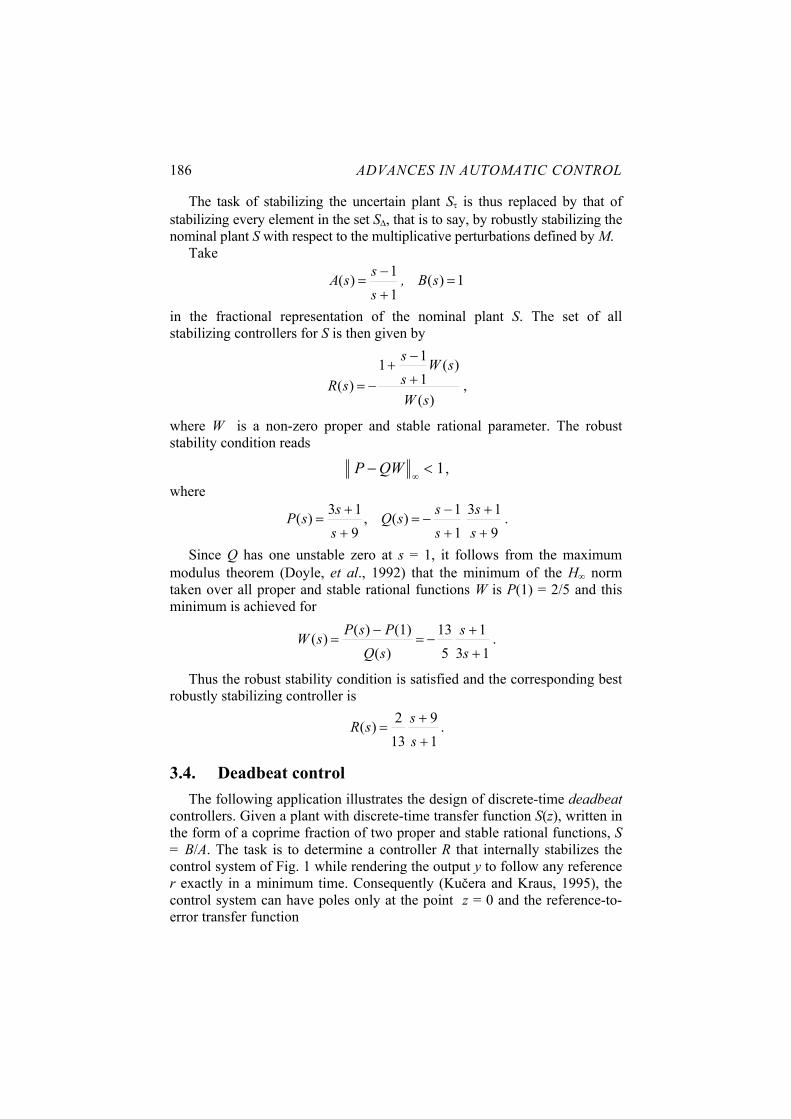
ADVANCES IN AUTOMATIC CONTROL 186
The task of stabilizing the uncertain plant Sτ is thus replaced by that of stabilizing every element in the set S∆, that is to say, by robustly stabilizing the nominal plant S with respect to the multiplicative perturbations defined by M. Take
1)(11)( =
+
−= sB,
sssA
in the fractional representation of the nominal plant S. The set of all stabilizing controllers for S is then given by
)(
)(111
)(sW
sWss
sR +
−+
−= ,
where W is a non-zero proper and stable rational parameter. The robust stability condition reads
1<−∞
QWP , where
913
11)(,
913)(
+
+
+
−−=
+
+=
ss
sssQ
sssP .
Since Q has one unstable zero at s = 1, it follows from the maximum modulus theorem (Doyle, et al., 1992) that the minimum of the H∞ norm taken over all proper and stable rational functions W is P(1) = 2/5 and this minimum is achieved for
131
513
)((1))()(
+
+−=
−=
ss
sQPsPsW .
Thus the robust stability condition is satisfied and the corresponding best robustly stabilizing controller is
19
132)(
+
+=
sssR .
3.4. Deadbeat control The following application illustrates the design of discrete-time deadbeat controllers. Given a plant with discrete-time transfer function S(z), written in the form of a coprime fraction of two proper and stable rational functions, S = B/A. The task is to determine a controller R that internally stabilizes the control system of Fig. 1 while rendering the output y to follow any reference r exactly in a minimum time. Consequently (Kučera and Kraus, 1995), the control system can have poles only at the point z = 0 and the reference-to-error transfer function

Parametrization of stabilizing controllers with applications 187
SR
H+
=1
1
must be a polynomial of least degree possible in z –1.
In the control system so designed, the polynomial H is given by the formula QWPBWXAH −=−= :)(
and its degree can be minimized by a choice of W: it suffices to identify W with the quotient of P/Q so that H becomes the remainder. To illustrate, consider a discrete-time integrator plant
1
1
(1 ε) (1 ε)( )
1 1z z
S zz z
−ε + − ε + −= = −− −
sampled at the unit rate and displacement ε of input and output sampling instants, with 0 < ε ≤ 1. The Bézout equation admits a solution
111 −=−−+= zzY,zzX )(ε)(1)( .
The set of all stabilizing controllers that allocate the closed loop poles to the point z = 0 is
Wzzz
WzzzzR
111
111
])(1[)(11
)1()(
−−−++−−+
−−−−−=
εεε
for an arbitrary polynomial W(z – 1). The resultant transfer function from r to e is
WzzzzzH 11111(1 −−+−−−+−= −−−−− ]ε)(1)[ε(1 ]ε)(1)[1)( 1z .
Taking the quotient of the polynomial division of 11 −−+ zε)(1 by 21 −−+− zz ε)(1ε gives the parameter W = 0; hence the optimal controller
1
1
)(11)(
−−+
−=
z
zzRε
and the polynomial
H(z) = ]ε)(1)[1 11(1 −−+−− zz .
The tracking error will vanish in three sampling periods.
3.5. Stabilization subject to input constraints Most plants have inputs that are subject to hard limits on the range of variations that can be achieved. The effects of actuator saturation on a control system are poor performance and/or instability. Stabilization subject

ADVANCES IN AUTOMATIC CONTROL 188
to input constraints can be formulated either as a local stabilization, when saturation is avoided for a set of initial states and the control system behaves as a linear one, or as a global stabilization, when saturation is allowed to occur and the control system is nonlinear. Consider the saturation avoidance approach. Given a discrete-time plant
0xzTzuzSzy )()()()( +=
with the input
...zuzuuzu +++= −− 22
110)(
subject to the constraints
...,,,k,uuu k 210=≤≤− +− ,
where u+ and u – are positive constants and x0 is the initial state. The task is to find a controller (zero initial state assumed) of the form
)()()( zyzRzu −=
such that the control system is locally asymptotically stable for any initial state x0 of the plant within a given polyhedron : nNxxPN ≤= , where N is a matrix and n is a vector. Denote S = B/A and T = C/A the fractional representation of the plant. The control sequence in a stable feedback system is
0xAWYCu )( −= .
Taking W in the form of a power series around the point z = ∞
...zpzpzW ++= −− 22
11)(
shows that the control sequence is an affine function of the parameters p1, p2, … of the form
...,,k,x...,p,p 21021 == )(kk Mu ,
and satisfies the given constraint if x0 belongs to the polyhedron )(: mxppMxPM ≤= ,..., 21 , where
=
−
−=
−
+
−
+
uuuu
m,,...p,pM
,...p,pM,...p,pM
,...p,pM
,...p,pM)(
)()(
)(
)(
212
212
211
211
21 .

Parametrization of stabilizing controllers with applications 189
Now x0 is in PN , so that PN must be contained in PM. Applying the Farkas lemma (Henrion, et al., 2001), one concludes that the stabilization problem has a solution if and only if there exists a matrix P with non-negative entries and real numbers p1, p2, … such that
mPnMPN ≤= ,,...p,p )( 21 .
This is a linear program for P and p1, p2, … . The stabilizing controller is then obtained by putting
...zpzpzW +−+−= 22
11)( .
If the power series W is approximated by a polynomial, then the program has a finite dimension. To illustrate, consider the plant described by the input-output and state-output transfer functions
11 21
2211
−− −=
−=
zT,
zS )()( zz .
The plant input is constrained as
...,,k,uk 2111 =≤≤− .
and the initial state x0 belongs to the polyhedron
≤
− 3
13
1
11
x:PN (that is, |x0| ≤ 1/3).
The set of stabilizing controllers is found to be
)(
()()(zW
zWzzzR+
−−=
−−
1
)212 11
and the corresponding control sequence is
011 224( xzWzzzu )]()(1[) −−−−−= .
Now start with W(z) = 0 and check whether the resulting linear program for P is feasible:
≤
−=
− 1
144
11
313
1P,P .
It is not, hence no controller of order 1 stabilizes the plant.

ADVANCES IN AUTOMATIC CONTROL 190
Proceed by choosing W(z) = p1 z –1 and check whether the resulting linear program for p1 and P is feasible:
[ ] [ ]1
31 1 1 1 1
3
14 2 4 2 4 4 , 1 1 1 1
1T TP p p p p P
= − − + − ≤ −
.
It is, and the solution
18 0 8 02 1,0 8 0 83 3
T
p P
= − =
furnishes the stabilizing controller
1
11
5122
−
−−
+
−=
z.zzzR )( .
The actual polyhedron of stabilizable initial states is
[ ] [ ]01: 8 8 8 8 1 1 1 13
T TMP x− − ≤ (that is, |x0| ≤ 3/8)
and it includes PN as a proper subset. The successive selection of a feasible parameter results in the increase of the order of the stabilizing controller. This points out to a potential weakness of the design procedure based on parametrization: each time an additional design specification is achieved, the order of the controller is increased.
4. Conclusions The parametrization of internally stabilizing controllers can easily be extended to multi-input multi-output systems (Vidyasagar, 1985). Rational matrices are represented as „matrix fractions“, that is to say, as the left and right factorizations
LLPP BAABS 11 −− ==
of two proper and stable rational matrices, where PA and PB are right coprime and LA and LB are left coprime. The set of all internally stabilizing controllers is given by
)()())(( 11LLLLPPPP WAYWBXWBXWAYR +−=−+= −− ,
where the proper and stable rational matrices LX , LY and PX , PY satisfy the Bézout identity
IAYBX
XYBA
PP
PP
LL
LL =
−
−

Parametrization of stabilizing controllers with applications 191
and W is a proper and stable rational matrix parameter (Kučera, 1975; Youla, et al., 1976b). It is interesting to note that the set of internally stabilizing controllers can be parametrized also for plants with irrational transfer functions. This is possible whenever such a transfer function is expressed in the form of a fraction of two coprime proper and stable rational functions. This property is by no means evident (Vidyasagar, 1985) and it holds, for instance, for transfer functions having a finite number of singularities in 0Re ≥s , each of which is a pole. Even more striking is the observation that internally stabilizing controllers can be parametrized for nonlinear plants, where transfer functions no longer exist. The key condition is again the possibility of factorizing the nonlinear mapping that defines the plant into two „coprime“ mappings, one of them representing a stable system while the other one representing the inverse of a stable system (Hammer, 1985). Technical assumptions may prevent one from parametrizing the entire set of internally stabilizing controllers; still, the subset may be large enough for practical purposes. The parametrization of all stabilizing controllers is a result that launched an entire new area of research and that has ultimately become a new paradigm for the design of optimal and robust control systems. Being of algebraic nature (Kučera, 1993), it is a result of high generality and elegance. The stabilizing controllers are obtained by solving a linear equation. This is not because the plant to be controlled is linear but because it is an element of the ring of fractions defined over the ring of stable plants (Vidyasagar, 1985). The requirement of stability is thus expressed as one of divisibility in a ring: an element a divides an element b if there exists an element x satisfying ax = b. That is why x is the solution of a linear equation. There is a dual result: the parametrization of all plants that can be stabilized by a fixed controller. This result is useful in system identification. In fact, the (difficult) problem of closed-loop identification of the plant becomes a (simple) problem of open-loop identification of the parameter, as discussed by Anderson (1998). Consequently, the parametrization may facilitate the study of dual control.
References Anderson, B.D.O. (1998). From Youla-Kucera to identification, adaptive and nonlinear
control. Automatica, 34, 1485-1506.
Desoer, C.A., R.W. Liu, J. Murray and R. Saeks (1980). Feedback system design: The fractional representation approach to analysis and synthesis. IEEE Trans. Auto. Control, 25, 399-412.
Doyle, J.C., B.A. Francis and A.R. Tannenbaum (1992). Feedback Control Theory. Macmillan, New York.

ADVANCES IN AUTOMATIC CONTROL 192
Hammer, J. (1985). Nonlinear system stabilization and coprimeness. Int. J. Control, 44, 1349-1381.
Henrion, D., S. Tarbouriech and V. Kučera (2001). Control of linear systems subject to input constraints: a polynomial approach. Automatica, 37, 597-604.
Kučera, V. (1974). Closed-loop stability of discrete linear single variable systems. Kybernetika, 10, 146-171.
Kučera, V. (1975). Stability of discrete linear feedback systems. In: Proc. 6 th IFAC World Congress, Vol. 1, Paper 44.1. Pergamon, Oxford.
Kučera, V. (1979). Discrete Linear Control: The Polynomial Equation Approach. Wiley, Chichester.
Kučera, V. (1993). Diophantine equations in control – a survey. Automatica, 29, 1361-1375.
Kučera, V. (2002). Parametrization of stabilizing controllers. In: Proc. 8th IEEE International Conference on Methods and Models in Automation and Robotics, 87-94. Politechnika Szczecińska, Szczecin.
Kučera V. and F.J. Kraus F. J. (1995). FIFO stable control systems. Automatica, 31, 605-609.
Newton, G.C., L.A. Gould and J.F. Kaiser (1957). Analytic Design of Linear Feedback Controls. Wiley, New York.
Strejc, V. (1967). Synthese von Regelungssystemen mit Prozessrechner. Akademie-Verlag, Berlin.
Vidyasagar, M. (1985). Control System Synthesis: A Factorization Approach. MIT Press, Cambridge.
Youla, D.C., J.J. Bongiorno and H.A. Jabr (1976a). Modern Wiener-Hopf design of optimal controllers, part I: the single-input case. IEEE Trans. Auto. Control, 21, 3-14.
Youla, D.C., H.A. Jabr and J.J. Bongiorno (1976b). Modern Wiener-Hopf design of optimal controllers, part II: the multivariable case. IEEE Trans. Auto. Control, 21, 319-338.
Zhou, K. and J.C. Doyle (1998). Essentials of Robust Control. Prentice-Hall, Upper Saddle River.

METHODOLOGY FOR THE DESIGNOF FEEDBACK ACTIVE VIBRATIONCONTROL SYSTEMS
Ioan Dore Landau, Aurelian Constantinescu,Daniel Rey, Alphonse FrancoLaboratoire d’Automatique de GrenobleENSIEG, BP 46, 38402 Saint Martin d’Heres, Francefax: + 33 (0)4 76 82 62 44e-mail: [email protected]
Patrice LoubatHutchinson - Centre de RechercheRue Gustave Nourry, BP 31, 45120 Chalette-sur-Loing, France
Abstract This paper presents an integrated methodology for feedback control ofactive vibration attenuation systems. The basic steps of the method-ology are: open loop identification of the secondary path, design of arobust digital controller, identification in closed loop of a ”control ori-ented” model, redesign of the controller based on the closed loop identi-fied model and controller reduction. The feasability of this methodologyis illustrated by its application on the Hutchinson active suspension.
Keywords: active control, active suspension, feedback control, closed loop identifi-cation, controller order reduction.
1. IntroductionFeedback is used in active vibration control mainly for three reasons:
Absence of a measurement correlated with the vibration source(which is necessary for feedforward control).Wide band vibration attenuation.Potential robustness of performances with respect to system modelvariations.
A number of techniques has been proposed for the design of feedbackcontrollers dedicated to active vibration attenuation [2, 3, 4]. Often an
193

194 ADVANCES IN AUTOMATIC CONTROL
adaptation loop is added for the tuning of the controller because eitherthe identified model is not enough accurate or because the designedcontroller is not enough robust. For more details on feedback used inactive vibration control see [4]-Chapter 3.
The key contributions of the present paper are related to:the identification of a good ”design model” by using up to dateopen loop and closed loop identification methods and model vali-dation tests;the design of a robust controller allowing to achieve severe perfor-mance constraints in terms of the frequency attenuation charac-teristics;the use of a recent developed efficient controller reduction methodpreserving the desirable properties of the nominal closed loop sys-tem.
For more details on this methodology see [1].To be specific we will start by presenting the system under consider-
ation for the experimental verification of the methodology.The structure of the system is presented in Fig. 1, a photo of the
system being presented in Fig. 2. The controller will act upon the piston(through a power amplifier) in order to reduce the residual force. Thesystem is controlled by a PC via an I/O card, the sampling frequencybeing 800Hz.
Figure 1. The active suspension system
The equivalent scheme is shown in Fig. 3.The system input, u(t) is the position of the piston, the output y(t)
being the residual force measured by a force sensor (see figs. 1, 3).The principle of the active suspension is to vary the system’s stiffness
in order to attenuate the vibrations generated by the part that we wantto isolate (primary force, disturbance). In our case, the primary forcehas been generated using a shaker controlled by a signal given by thecomputer.

Methodology for the design of feedback active vibration control systems 195
Figure 2. Active suspension system (photo)
We call primary path transfer function (q−d1C
D) the transfer function
between the signal sent to the shaker, p and the residual force y(t).
We call secondary path transfer function (q−d B
A) the transfer function
between the input of the system, u(t) and the residual force. The inputof the system being a position and the output a force, the secondarypath transfer function has a double differentiator behaviour.
Figure 3. Block diagram of the active suspension system
The frequency characteristic of the identified primary path model (theeffect of the disturbances on the output), between the excitation of theshaker and the residual force is shown in Fig. 4. The control objectiveis to minimize the modulus of the transfer function between the inputsignal of the shaker and the residual force at low frequencies, using afeedback control. In other words, to attenuate the first vibration mode,without amplifying the disturbance effect in low frequencies (below 31Hz) and minimizing the maximum amplification of the disturbances over35 Hz by distributing it through the high frequencies up to 200 Hz.

196 ADVANCES IN AUTOMATIC CONTROL
0 0.05 0.1 0.15 0.2 0.25 0.3 0.35 0.4 0.45 0.5−30
−20
−10
0
10
20
30
40Primary path identified model
f [Hz]
Mag
nitu
de [d
B]
Figure 4. The frequency characteristic of the primary path model (input: shaker’ssignal, output: residual force)
Assuming that a good model of the system is available, the difficultyin controller design comes from the constraints in low frequencies (noamplification is allowed below 31Hz). In our case the allowed amplifi-cation in the frequency region over 35Hz is ≤ 3dB. See for example [2]for less stringent frequency specifications.
The methodology proposed for the design of feedback active vibrationcontrol is illustrated in Fig.5.
The first stage is the open loop identification and validation of a dis-crete time model for the secondary path (between the piston’s positionand the residual force).
Then a controller based on this open loop identified model is designedand implemented (open loop based controller). The pole placement withshaping of the sensitivity functions by convex optimization is used forthe design [11].
Once the open loop based controller is implemented, an identificationin closed loop is carried out [8]. This allows to get a better design model,since identification in closed loop (using appropriate algorithms) willenhance the precision of the estimated model in the critical frequencyregions for control.
Then a re-design of the controller is done based on the closed loopidentified model (nominal closed loop based controller).
The nominal controller is then implemented and tested.The next stage is the reduction of the controller complexity, which can
be done using simulated or real data. The algorithms used for controllerreduction will preserve the desirable properties of the nominal closedloop system [9, 6].

Methodology for the design of feedback active vibration control systems 197
Figure 5. Design methodology
The last stage is a comparison in real time between the performancesof the nominal and reduced order controllers.
The paper is organized as follows: Section 2 will discuss the modelidentification (in open and in closed loop). Section 3 will present thecontroller design methodology. Section 4 will present the controller re-duction technique. Section 5 will illustrate the application of the designmethodology to the Hutchinson active vibration attenuation system.
2. Open and closed loop identificationFrom a practical point of view, the identification of a plant model is
the first thing to do for the design of a controller.The identification of a system is an experimental approach for esti-
mating a model of the real system. The identification procedure can bedivided in four different steps:

198 ADVANCES IN AUTOMATIC CONTROL
I/O data acquisition (under an experimental protocol).Estimation of the model complexity.Estimation of the model parameters and choice of the noise model.Validation of the identified model.
An important point in the identification of a system is the excitation sig-nal. In this paper we use as excitation signal a PRBS (Pseudo RandomBinary Sequence). See [10] for details.
2.1. Open loop identificationThe open loop identification algorithms minimize the error between
the output of the real system and the output of the estimated model.In other words, they try to estimate a model whose output fits as muchas possible the part of the output of the real system generated by theexcitation signal. For details on open loop identification and validationsee [10].
2.2. Closed loop identificationClosed loop identification can be used when a controller (i.e. based on
an open loop identified model) exists, in order to obtain a better modelof the real plant since the precision of the estimated model is improvedin the critical frequency regions for control. Of course, this requires touse specific algorithms.
K
P.A.A.
G
r
u
u y
y
CLε
+
+
+
−
−
−
K
G
p
+
+
Figure 6. Identification in closed loop
The closed loop identification algorithms minimize the error betweenthe true closed loop system and the adjustable predictor of the closedloop. The objective of the closed loop identification is to obtain a betterpredictor for the closed loop, using a better estimation of the plant

Methodology for the design of feedback active vibration control systems 199
model. The predictor of the closed loop is formed by the controller andthe estimated plant model (see Fig. 6). For more details on the closedloop identification see [7, 8].
3. Controller designThe method used in this paper for the computation of a robust digital
controller is the pole placement method with shaping of the sensitivityfunctions by convex optimization.
The combined pole placement/sensitivity function shaping methodconsists of placing the dominant closed loop poles, specifying some fixedparts of the controller and then adding auxiliary poles and controllerparts to fulfill specifications on the output and input sensitivity functionsby a convex optimization procedure [11].
3.1. Plant representation and controller structureThe structure of a linear time invariant discrete time model of the
plant (on which is based the design of the controller) is
G(z−1) =z−dB(z−1)
A(z−1), (1)
where:
d = number of sampling periods on the plant pure time delay;A = 1 + a1z
−1 + . . . + anAz−nA ;
B = b1z−1 + . . . + bnB
z−nB .
The controller to design is a RS-type controller (see Fig. 7). The sensi-
Figure 7. Structure of RS-controller
tivity functions for the closed loop are:

200 ADVANCES IN AUTOMATIC CONTROL
the output sensitivity function (the transfer function between theperturbation p1(t) and the output y(t)):
Syp(z−1) = −A(z−1)S(z−1)P (z−1)
; (2)
the input sensitivity function (the transfer function between theinput of the plant u(t) and the output y(t)):
Sup(z−1) = −A(z−1)R(z−1)P (z−1)
, (3)
where P (z−1) are the poles of the closed loop.
3.2. Design problem formulationThe problem may be formulated as follows: Given a nominal plant
model Gnom =z−dBnom
Anomobtained by identification, define:
the fixed parts of the controller (HR and HS);the desired closed loop behaviour (the dominant closed loop polesPD and the acceptable region for the optimized ones);the desired upper bounds Wx(ω) for the modulus of the sensitivityfunctions (performance and robustness objectives);an objective to be minimized.
3.3. Controller parameterizationThe parameterization used for the controller is the Youla-Kucera Pa-
rameterization:
R
S=
HR(R0 + AnomHSQ)HS(S0 − z−dBnomHRQ)
, (4)
where the fixed parts of the controller, HR, HS and Anom, Bnom arepolynomials of z−1.
The central controller (Q = 0) can be obtained by solving the Bezoutequation for R0 and S0:
AnomHSS0 + z−dBnomHRR0 = PD, (5)
where PD is a stable polynomial containing the desired dominant closedloop poles. Expressing Q as a fraction of polynomials β and α (with αstable), we obtain:

Methodology for the design of feedback active vibration control systems 201
R
S=
HR(R0α + AnomHSβ)HS(S0α − z−dBnomHRβ)
(6)
Pnom = AnomS + z−dBnomR = PDα, (7)
where the zeros of PD are the fixed closed loop poles and the zeros of αare the additional (optimized) ones.
Using the parameterization and constraint formulation presented above,a controller (R and S) with the required properties may be obtained byconvex optimization. For more details on the optimization proceduresee [11].
4. Controller reductionThe design of a robust controller (see Section 3) leads normally to
high order controllers. There exist two main approaches to obtain areduced order controller:
to reduce the order of the plant model and then to compute a loworder controller based on the reduced model;
to compute a high order controller based on the nominal plantmodel, and then to reduce the order of the obtained controller.
The second approach seems more appropriate because the approximationis done in the final step of the controller design. In addition, the firstapproach in this case did not allowed to obtain enough simple controllers.
Identification in closed loop offers an efficient methodology for thecontroller order reduction. The most important aspect of the controllerreduction is to preserve as much as possible the desirable closed loopproperties.
One block diagram for reduced order controller identification is pre-sented in Fig. 8. The simulated nominal closed loop system (the upperpart of Fig. 8) is constituted by the nominal designed controller, K andthe best identified plant model, G. The lower part is constituted bythe estimated reduced order controller, K and the plant model, G. Itis assumed that the nominal controller stabilizes the real plant and theidentified plant model.
The parametric adaptation algorithm will try find the best reducedorder controller of a given order which will minimize the closed loop inputerror (the difference between the input of the plant model generated inthe nominal simulated closed loop, u, and the input of the plant modelgenerated by the closed loop using the reduced order controller, u).
Identification of a reduced order controller can also be done using realdata [9].

202 ADVANCES IN AUTOMATIC CONTROL
Figure 8. Closed-loop identification of reduced order controllers using simulateddata (input matching: CLIM)
One can also consider as an objective for controller order reductionto minimize the closed loop error between the plant output generatedin the nominal simulated closed loop and the plant output generated inthe closed loop using the reduced order controller (CLOM algorithms)[5].
For more details on the algorithms see [9, 5, 6].An important aspect for the reduction procedure, from the valida-
tion point of view, is that the reduced order controllers should stabilizethe nominal model, G, and they should give sensitivity functions whichare close to those obtained with the nominal controller in the criticalfrequency regions for performance and robustness [9].
5. Application of the designed methodology toan active suspension
The design methodology proposed in the previous sections will beillustrated on an active suspension. The active suspension has beenpresented in the Section 1 of this paper.
The primary path transfer function has been identified in open loop.The excitation signal sent at the input of the shaker is a PRBS with 10cells shift register and the frequency divider p = 2. For the identificationwe used 2048 data points.
The primary path identified model has the following orders: nC = 12,nD = 9, delay d1 = 2. The frequency characteristic of the identifiedmodel is presented in Fig. 4.

Methodology for the design of feedback active vibration control systems 203
One can see that there exist several vibration modes, the first one(that we desire to attenuate) being at 31.5Hz with a damping factor0.093.
We shall present below the results obtained, step by step.
5.1. Step 1: Open loop identification of a discretemodel for the secondary path
The excitation signal sent at the input of the system (the piston) isa PRBS with 9 cells shift register and the frequency divider p = 4. Forthe identification we used 2048 data points.
The reason of using a frequency division p = 4 is that we are interestedto obtain a good model in low frequencies, a PRBS with p = 4 having ahigher energy in low frequencies. See [10] for details.
The identified model of the secondary path has the following orders:nA = 12, nB = 11, delay d = 2, and it has been identified using theRecursive Maximum Likelihood method with a variable forgetting factor.
The frequency characteristic of the identified model is presented inFig. 9 (thin line), the first vibration mode being at 31.98Hz with adamping factor 0.078. As we can see, there are 6 vibration modes fromwhich 5 are very low damped (< 0.078). We have chosen the best modelfrom the point of view of the open loop validation techniques.
0 50 100 150 200 250 300 350 400−40
−30
−20
−10
0
10
20
30
40Active suspension identified models (open and closed loop)
Mag
nitu
de [d
B]
f [Hz]
Open loop identified modelf1 = 31.98 Hz; xi = 0.078f2 = 145.08 Hz; xi = 0.712f3 = 158.59 Hz; xi = 0.040f4 = 239.56 Hz; xi = 0.037f5 = 279.19 Hz; xi = 0.028f6 = 364.73 Hz; xi = 0.016
Closed loop identified modelf1 = 32.76 Hz; xi = 0.085f2 = 107.70 Hz; xi = 0.641f3 = 157.13 Hz; xi = 0.062f4 = 221.92 Hz; xi = 0.024f5 = 273.02 Hz; xi = 0.033f6 = 371.13 Hz; xi = 0.045
Figure 9. The frequency characteristics of the secondary path model (input: pistondisplacement, output: residual force)

204 ADVANCES IN AUTOMATIC CONTROL
5.2. Step 2: Design of a robust controllerHaving now an open loop identified model, identified in Step 1, one
can pass to the computation of a robust digital controller. We used themethodology presented in Section 3.
In order to compute the controller, we fixed a pair of dominant polesat the frequency of the first vibration mode of the open loop identifiedmodel with a damping factor 0.8. We introduced also some fixed partsin the controller (in HR):
HR = 1+q−1 (assures the opening of the loop at 0.5fs - robustnessreason);a pair of zeros at 215Hz with a damping factor 0.01 (assures a verylow gain of the controller at the frequency where the energy of thePRBS used for identification is low (0.25fs) and where thereforeone has an uncertainty on the model);a pair of zeros at 20.5Hz with a damping factor 0.01 (assuresthe opening of the loop in low frequencies, because of the factthat attenuating the first vibration mode may other way produceamplification in low frequencies (below 31Hz)).
The constraints on the sensitivity functions are the templates presentedin Fig. 10. The template on the Syp function has been established as afunction of the desired disturbance rejection, the one on Sup is a functionof the saturation problems of the actuator. The template on Syp is at−12dB at the frequency corresponding to the first vibration mode andat 0dB at the frequencies over 35Hz (up to 150Hz), because we shouldlike a very little amplification in this frequency region. We ask a littlevalue of Sup at 0.25fs because of the uncertainties of the identified modelin this frequency region. The objective is to minimize the Syp sensitivityfunction in the regions of interest (see the template) without stickingout from the template on Sup.
The resulting controller (the nominal one) has the following complex-ity (the orders of polynomials R and S): nR = 27, nS = 28. The outputsensitivity function Syp, respectively the input one, Sup, are presentedin Fig. 10. From Fig. 10 one can see that we obtain a good disturbancerejection (low magnitude of Syp) at the frequency corresponding to thefirst vibration mode (≈ 31Hz) and that we do not amplify at all in lowfrequencies. The maximum amplification over 31Hz is below 3dB.
5.3. Step 3 and 4: Controller implementation andclosed loop identification
Having now the nominal controller (which stabilizes also the realplant), computed at Step 2, we can proceed to the closed loop iden-

Methodology for the design of feedback active vibration control systems 205
50 100 150 200 250 300 350−15
−10
−5
0
5
10
Mag
nitu
de [d
B]
Output sensitivity
Model Template
0 50 100 150 200 250 300 350 400
−40
−30
−20
−10
0
10
Frequency [Hz]
Mag
nitu
de [d
B]
Input sensitivity
Figure 10. Sensitivity functions
Table 1. Closed loop validation results
Plant model Open loop Closed loop
C.L. Err. var. 1.5368 0.1477
|RN(i)|max 0.4802 0.0340
Vinnicombe 0.7624 0.3587
tification of the secondary path in order to improve the quality of theopen loop identified model (see Step1).
We use the same excitation signal from the open loop identification(Step 1) and we add it on the input of the system (the piston), which isnow in feedback with the nominal controller (see Fig. 3)
We identify a model having the same complexity as the open loopone. We use the F-CLOE (Filtered Closed Loop Output Error) method[8].
The closed loop validation results for the open loop, respectivelyclosed loop identified models, are presented in Table 1. The first twolines give the variance of the residual closed loop error and the maxi-mum of the normalized cross correlations between estimated output andresidual closed loop error. The third line gives the Vinnicombe distancebetween the identified transfer function of the real closed loop systemand the closed loop transfer function of the simulated closed loop (nomi-nal controller + model to validate). For details on closed loop validationand Vinnicombe distance see [8, 10], and [12], respectively.
One can see that the closed loop identified model validates better thanthe open loop one.

206 ADVANCES IN AUTOMATIC CONTROL
5.4. Step 5: Re-design of a controllerHaving now a better model of the real system, we compute a robust
digital controller based on this model, in order to improve the perfor-mances of the controller on the real system.
The controller based on the closed loop identified model is obtainedusing the same methodology and the same constraints (templates on thesensitivity functions) imposed in Step 2.
5.5. Step 6: Performance testsIn order to test the performances of the nominal controller on the real
system, we present the spectral density of the residual force in open andin closed loop (see Fig. 11). One can see an attenuation of about 7dB
0 50 100 150 200 250 300 350 400−50
−40
−30
−20
−10
0
10
f [Hz]
Spectral density of the residual force in open and in closed loop
Vrm
s [d
B]
Open loop Closed loop (nominal controller)
Figure 11. Spectral density of the residual force in open and in closed loop
at the frequency corresponding to the first vibration mode (≈ 31Hz),without any amplification in low frequencies. The tolerated amplifica-tion (3 dB) over 35 Hz has been verified, so the controller obtainedaccomplished the desired performances.
5.6. Step 7: Controller reductionIn order to do the order reduction of the nominal controller, we shall
give the results obtained using the CLIM direct reduction method pre-sented in Section 4, based on simulated data. The plant model usedis the closed loop identified model. We use as external input a PRBSgenerated by 10 cells register and with a frequency divider of p = 2. Weuse 4096 data points and a variable forgetting factor. For more details,see [9, 6].

Methodology for the design of feedback active vibration control systems 207
We present the reduction results by showing the sensitivity functions(Syp and Sup in figs. 12, 13) for the nominal controller Kn with nR =27, nS = 28 and for three reduced order controllers: K1 with nR = 19,nS = 20, K2 with nR = 12, nS = 13 and K3 with nR = 9, nS = 10respectively (a fixed part HR = 1+q−1 has been imposed in the reducedorder controllers). K3 controller has a lower complexity than the poleplacement one.
0 0.05 0.1 0.15 0.2 0.25 0.3 0.35 0.4 0.45 0.5−8
−6
−4
−2
0
2
4Syp − Output sensivity function
f / fs
dB
Nominal (nR = 27, nS = 28)nR = 19, nS = 20 nR = 12, nS = 13 nR = 9, nS = 10
Figure 12. Output sensitivity for the active suspension (controller reduction usingCLIM algorithm on simulated data)
0 0.05 0.1 0.15 0.2 0.25 0.3 0.35 0.4 0.45 0.5−50
−40
−30
−20
−10
0
10
Sup − Input sensivity function
f / fs
dB
Nominal (nR = 27, nS = 28)nR = 19, nS = 20 nR = 12, nS = 13 nR = 9, nS = 10
Figure 13. Input sensitivity for the active suspension (controller reduction usingCLIM algorithm on simulated data)

208 ADVANCES IN AUTOMATIC CONTROL
Note: The reduced controller K2 corresponds to the complexity ofthe pole placement controller.
One can see the closeness of the sensitivity functions.Similar results are obtained by using real data for the reduction of the
controller complexity.
5.7. Step 8: Performance testsTo illustrate the performances of the resulting controllers (Kn, K1,
K2 and K3) on the real system, the spectral density of the residualacceleration in open and in closed loop is shown in Fig. 14. The spec-tral densities obtained in closed loop operation are compared to thosecorresponding to the open loop operation.
The performances of the reduced order controllers are close to thatof the nominal controller and all achieve a significant reduction of thevibrations around the first vibration mode of the plant model.
0 50 100 150 200 250 300 350 400−50
−40
−30
−20
−10
0
10
f [Hz]
Spectral density of the residual acceleration in opened and in closed loop (simulated data)
Vrm
s [d
B]
Open loop Nominal (nR = 27, nS = 28)nR = 19, nS = 20 nR = 12, nS = 13 nR = 9, nS = 10
Figure 14. Spectral density of the residual acceleration in open and in closed loop(controller reduction using CLIM algorithm on simulated data)
6. ConclusionsThe methodology presented in this paper allowed to design a feedback
control for an active vibration system and has been successfully testedin real time.
The real system has been identified in open and in closed loop. Theresulting controller accomplished the desired performances. The nominalcontroller has been simplified by a procedure preserving the closed loopproperties. The reduced order controller (19 parameters instead of 55)gives very close results to those of the nominal controller.

Methodology for the design of feedback active vibration control systems 209
References[1] Constantinescu, A. (2001). Commande robuste et adaptative d’une suspension
active. These de doctorat. Institut National Polytechnique de Grenoble.
[2] Curtis, A. R. D. (1997). A methodology for the design of feedback control sys-tems for the active control of sound and vibration. Active 97 pp. 851–860. Bu-dapest - Hungary.
[3] Friot, E. (1997). Optimal feedback control of a radiating plate under broadbandacoustic loading. Active 97 pp. 873–884. Budapest - Hungary.
[4] Fuller, C. R., S. J. Elliott and P. A. Nelson (n.d.). Active control of vibration.Academic Press. London.
[5] Karimi, A. and I. D. Landau (2000). Controller order reduction by direct closedloop identification (output matching). Proceedings IFAC Symp. ROCOND 2000,Prague.
[6] Landau, I. D., A. Karimi and A. Constantinescu (2001). Direct controller orderreduction by identification in closed loop. Automatica (37), 1689–1702.
[7] Landau, I. D. and A. Karimi (1997a). An output error recursive algorithm forunbiased identification in closed loop. Automatica 33(5), 933–938.
[8] Landau, I. D. and A. Karimi (1997b). Recursive algorithms for identification inclosed loop: a unified approach and evaluation. Automatica 33(8), 1499–1523.
[9] Landau, I. D. and A. Karimi (2000). Direct closed loop identification of reducedorder controllers (input matching). Proceedings of IFAC Symp. SYSID 2000, S.Barbara.
[10] Landau, I. D., R. Lozano and M. M’Saad (1997). Adaptive control. Springer.London.
[11] Langer, J. and I. D. Landau (1999). Combined pole placement/sensitivityfunction shaping method using convex optimization criteria. Automatica35(6), 1111–1120.
[12] Vinnicombe, G. (1993). Frequency domain uncertainty and the graph topology.IEEE Trans. on Automatic Control 38, 1371–1383.


FUTURE TRENDS IN MODEL PREDICTIVE CONTROL
Corneliu Lazar “Gh. Asachi” Technical University of Iaşi Department of Automatic Control and Industrial Informatics Bd. D. Mangeron nr. 53A, 700050 Iaşi, Romania E-mail:[email protected]
Abstract Model predictive control is a control technique in which a finite horizon optimal control problem is solved at each sampling instant to obtain the control input. The measured state is used as initial state and only the first control of the calculated optimal sequence of controls is applied to the plant. A key advantage of this form of control consists in its ability to cope with complex systems and hard constraints on controls and states. This resulted in a wide range of applications in industry, most of them in the petro-chemical branch. In this survey, a selected history of model predictive control is presented, with the purpose to outline the principles of this control methodology and to analyze the progress that has been made. The initial predictive control algorithms, mainly based on input/output models, are recalled in the introduction and then we focus on the more recent work done in nonlinear model and hybrid model predictive control. The stability problem and the computational aspects are discussed to formulate some fruitful ideas for the future research.
Keywords: model predictive control, discrete-time systems, nonlinear systems, hybrid systems, constraints, stability
1. Introduction Model Predictive Control (MPC) is a control strategy that offers attractive solutions, already successfully implemented in industry, for the regulation of constrained linear or nonlinear systems and, more recently, also for the regulation of hybrid systems. Within a relatively short time, MPC has

ADVANCES IN AUTOMATIC CONTROL 212
reached a certain maturity due to the continuously increasing interest shown for this distinctive part of control theory, and this has been illustrated by the prolific literature on this subject, including (Garcia et al., 1989; Qin and Badgwell, 1997; Allgöwer et al., 1999; Camacho and Bordons, 1999; Morari and Lee, 1999; Mayne et al., 2000; Rawlings, 2000; Maciejowski, 2002). The reason for the rapid development of MPC algorithms mainly consists in the intuitive way of addressing the control problem. In comparison with conventional control, which uses a pre-computed control law, predictive control is built around the following key principles: the explicit use of a process model for calculating the future behavior of the plant, the optimization of an objective function subject to constraints (which yields an optimal control sequence) and the receding horizon control strategy. The MPC methodology involves solving on-line an open-loop optimal control problem subject to input, state and/or output constraints. The graphical interpretation of this concept is depicted in Fig. 1.
Figure 1. Graphical interpretation of model predictive control
At each sampling instant k, the measured variables and the process model (linear, nonlinear or hybrid) are used to predict the future behavior of the controlled plant over a specified discrete-time horizon called prediction horizon (N). This is achieved considering a future control scenario as the input sequence applied to the process model, which must be calculated such that certain desired (imposed) objectives are fulfilled. To do that, a cost function is minimized subject to constraints, yielding an optimal control sequence over a discrete-time horizon named control horizon (Nu). Note that Nu ≤ N and if the control horizon is strictly smaller than the prediction horizon, the control input will be kept constant after Nu sampling time

Future trends in model predictive control 213
instants. According to the receding horizon control strategy, only the first element of the computed optimal control sequence is then applied to the plant. The original MPC algorithms, addressing linear systems exclusively, utilized only input/output models. In this framework, several solutions have been proposed both in the industrial world, IDCOM – Identification and Command (later MAC – Model Algorithmic Control) at ADERSA (Richalet et al., 1978) and DMC – Dynamic Matrix Control at Shell (Cutler and Ramaker, 1980), which use step and impulse response models, and in the academic world (the adaptive control branch) MUSMAR – Multistep multivariable adaptive regulator (Mosca et al., 1984), predictor-based self tuning control (Peterka, 1984), EHAC – Extended Horizon Adaptive Control (Ydstie, 1984), EPSAC – Extend Predictive Self-Adaptive Control (De Keyser and Van Cauwenberghe, 1985). Other MPC algorithms were also developed later on, from which the most significant ones are GPC – Generalized Predictive Control (Clarke et al., 1987) and UPC – Unified Predictive Control (Soeterboek, 1992). Next, the MPC algorithms have been designed for state-space models and extensions to nonlinear models followed shortly. In the framework of Nonlinear Model Predictive Control (NMPC), several alternatives have been studied and implemented with good results, such as dual-mode NMPC (Michalska and Mayne, 1993), quasi-infinite horizon NMPC (Chen and Allgöwer, 1996; Chen and Allgöwer, 1998) or contractive NMPC (de Oliveira Kothare and Morari, 2000). Also, a more recent stabilizing NMPC algorithm has been presented in (Magni et al., 2001). The first MPC approach to the control of hybrid systems has been reported quite recently in (Bemporad and Morari, 1999). Since then, several MPC schemes have been proposed for particular relevant classes of hybrid systems, such as the ones in (Bemporad et al., 2000; De Schutter and Van den Boom, 2001; De Schutter et al., 2002; Mayne and Rakovic, 2002; Lazar and Heemels, 2003). By now, the linear MPC theory is quite mature. Important issues such as on line computations, the interplay between modeling-identification and control, and system theory subjects like stability and robustness are well defined. In the sequel, we will only focus on the NMPC and the MPC framework for hybrid systems and the associated problems.
2. NMPC - Basic concepts and problem formulation When nonlinear systems (models) are employed, despite the slightly different problem formulation, the basic concepts are still the key principles of predictive control. The use of a nonlinear model only complicates the finite horizon optimal control problem that has to be solved on-line. Consider the general discrete-time nonlinear systems described by the

ADVANCES IN AUTOMATIC CONTROL 214
difference equation:
),(1 kkk uxfx =+ (1)
subject to input and state constraints of the form:
,0 , 0 , ≥∀∈≥∀∈ kX xkUu kk (2)
where nkx ℜ∈ is the state vector, m
ku ℜ∈ is the control input vector and f(.) = [f 1(.), f 2(.), …. , f n(.)]T is a vector containing smooth nonlinear functions of their arguments, which are zero at zero. In the simplest form, the sets U and X are defined by:
maxminmaxmin | ,| xxxxXuuuuU kn
kkm
k ≤≤ℜ∈=≤≤ℜ∈= ,(3)
where umin, umax, xmin, xmax are given constant vectors. The control objective is to regulate the state x to a desired equilibrium point xr. As any equilibrium point xr can be reduced to the origin via a suitable change of coordinates, we consider for the rest of the paper that the goal is to steer system (1) to the origin, while fulfilling the constraints (2). The predictive control approach to the above stated control problem leads to the minimization of the cost function:
( ) ( )∑−
=+=
1
0,),(
N
ikNkikikk xLuxFxJ u (4)
subject to:
1 ( , ), ,
, [0, ], [ , ],
, [0, ],u
kk k k k k k k k
u N ui k i k
i k
x f x u x x
u U i N u u , i N N
x X i N
+ = =
∈ ∈ = ∈
∈ ∈
(5)
where ] . . . [ |1|1|0 kNkkk uuu −=u are the manipulated controls, F(.) is the stage cost and L(.) is a suitable terminal state penalty term. The stage cost specifies the desired control performances and it is usually a quadratic function in x and u: ( ) i
Tii
Tiii RuuQxxuxF +=, (6)
with Q and R positive definite and symmetric weighting matrices. Note that, for simplicity, it is assumed that the prediction horizon N is equal to the control horizon Nu. Thus, the NMPC control problem can be stated as: Problem 1 Solve:

Future trends in model predictive control 215
kkkikikkk
xxNiXxN-iUuxJ =∈∈∈∈ /0// ]; ,0[ , ];1 ,0[ ,|),(min uu
, (7)
which yields the optimal control sequence
] . . . [ /1/1/0 kNkkk uuu −=u , (8)
and apply to plant (1) only the first element of (8). The initial condition from (5) shows that the system model used to predict the future in the controller is initialized by the actual system state. In general, at each time instant k the full state xk is assumed to be measured or must be estimated. Model-plant mismatch and disturbances are not represented in the optimization problem. In general it would be desirable to use an infinite prediction horizon, i.e.
∞=N , and to minimize the cost function (4) with L = 0, in order to achieve stability of the closed-loop system. However, the open-loop optimal control problem that must be solved on-line is often formulated using a finite prediction horizon, resulting thus in a finite parameterized problem which allows a (real-time) numerical solution of the nonlinear programming Problem 1. It is obvious that the shorter the prediction horizon is, the less time consuming are the calculations involved, so it is advantageous from a computational point of view to implement MPC schemes using short horizons. Still, the problem now consists in the fact that the actual closed-loop input and state trajectories will differ from the open-loop trajectories, even if no model mismatch and no disturbances are present. Moreover, it is by no means true that a repeated minimization of a finite horizon cost function in a receding horizon manner leads to an optimal solution also for the infinite horizon problem with the same stage cost F (Bitmead et al., 1990). In fact the two solutions differ significantly if a short horizon is utilized, which implies that there is no guarantee that the NMPC closed-loop system will be stable. Hence, when using finite horizons in standard NMPC, the employed cost function cannot be simply developed from the desired physical objectives.
2.1. NMPC algorithms with guaranteed stability The most perceptive way to achieve stability, when an NMPC algorithm is utilized to calculate the control law, is to choose an infinite prediction horizon. In this case, with the state available for measurement, no model mismatch and no disturbances it follows directly from Bellmann’s principle of optimality that the open-loop input and state trajectories calculated at a specific time instant k as a solution of the NMPC Problem 1, are in fact identical with the closed-loop trajectories of the nonlinear plant. This implies closed-loop stability because any feasible predicted trajectory goes to the origin. Since nearly all stability proofs for NMPC follow along the same basic steps as for the infinite horizon proof, at this point, it is worth mentioning the

ADVANCES IN AUTOMATIC CONTROL 216
key ideas: considering the cost function as a Lyapunov function, it is first shown that feasibility at one time instance does imply feasibility at the next time instance for the nominal case, in a second step, it is established that the cost function is strictly decreasing and thus the state and the input are converging to the origin, and finally, in a third step, asymptotic stability is established using the continuity of the cost function at the origin and its monotonicity properties. Unfortunately, an infinite horizon for the NMPC Problem 1 is only useful as a theoretical concept, because the solution of such a high dimension optimization problem is extremely difficult, if not impossible to obtain. Due to this reason, finite horizon approaches are preferred for NMPC, despite the inconsistencies between the open-loop predicted trajectories and the closed-loop actual trajectories mentioned above. Instead of using an infinite prediction horizon, stability is achieved / guaranteed by adding suitable constraints (not connected with physical restrictions or desired performance/ requirements) and penalty terms to the original cost function (4). Therefore, these extra conditions are referred as stability constraints. In the following, two representative finite horizons NMPC schemes with guaranteed stability are presented. Dual-mode NMPC This NMPC approach was introduced in (Michalska and Mayne, 1993) and consists in the use of two different controllers that are applied in different regions of the state space depending on the state being inside or outside of some terminal region that contains the origin. For the case in which the state is outside the terminal region an NMPC controller with a variable finite horizon is applied and, when the current state has entered the terminal region, a linear state feedback control law is employed. Thus, the proposed NMPC algorithm utilizes the following twofold control strategy:
0 / ,, .k k
kk k
u if xu
Kx if x∉Ω
= ∈Ω (9)
The terminal region Ω and the state feedback are calculated off-line such that the terminal region is a positive invariant region of attraction for the nonlinear system controlled by the linear state feedback algorithm and thus, the input and state constraints are satisfied with this linear controller in Ω. According to the dual-mode approach, when the state is outside Ω, the length N of the horizon is considered as an additional minimizer and Problem 1 to be solved, becomes:
/ / 0/,min ( , , ) | , [0, 1]; , [0, ];
kk k i k i k k ku N
J x u N u U i N - x X i N x x∈ ∈ ∈ ∈ = (10)
with the additional terminal inequality constraint
BNx Ω∈ , (11)

Future trends in model predictive control 217
which ensures that at the end of the horizon, the state has to lie on the boundary ΩB of the terminal region Ω. Starting from the outside of terminal region, the dual-mode NMPC controller guarantees the reaching of the terminal region boundary in a finite time. The close-loop stability is attained due to the use of a stabilizing local linear feedback control law. From the computational point of view, the dual-mode NMPC solution is more attractive because a inequality constraint is used, rather than a terminal equality constraint. The main drawback consists in the requirement to switch between control strategies and in determining the terminal region Ω. Quasi-infinite horizon NMPC The quasi-infinite horizon NMPC strategy was presented in (Chen and Allgöwer, 1996) and then further developed in (Chen and Allgöwer, 1998), where the inequality stability constraint
Ω∈Nx (12)
and the quadratic terminal penalty term
NTNN PxxxL =)( (13)
have been added to the standard NMPC Problem 1. The authors started from an infinite horizon cost function described by
∑∞
=
∞∞ =
0),(),(
iiikk uxFxJ u , (14)
where ∞ku is an infinite length control sequence. Splitting (14) in two parts,
Problem 1 can be recast as:
+= ∑∑∞
=
−
=∞∞
∞∞ Niii
N
iii
kkk
k
uxFuxFxJ ),(),(min),(min1
0uuu . (15)
The basic idea is that the final cost L is not a performance specification that can be chosen freely, but rather that the P matrix must be pre-computed such that the penalty term (13) is a good approximation of the second term in (15) (the infinite stage cost). Unfortunately, this is not usually feasible for general nonlinear systems, without introducing further restrictions. In particular, if the case is that the trajectories of the closed-loop system remain within some neighborhood of the origin (Ω) from the time instant k + N towards infinity, then, an upper bound on the second term of (15) exists. The terminal region Ω is built such that a local state feedback law similar to the one employed in dual-mode NMPC asymptotically stabilizes the nonlinear system in Ω. Moreover, it is shown in (Chen and Allgöwer, 1998) that if the terminal region Ω and the terminal penalty matrix P is chosen according to

ADVANCES IN AUTOMATIC CONTROL 218
Procedure 1 of (Chen and Allgöwer, 1998), then
∑∞
=≤
NiN
TNii PxxKxxF ),( , (16)
holds and the following equality is obtained
),(min),(min kkkk xJxJNkk
uuuu
=∞∞∞
, (17)
with J being the cost function as in the standard NMPC Problem 1. This implies that the optimal value of the finite horizon optimization problem bounds the value of the corresponding infinite horizon optimization problem, and thus asymptotic stability of the closed-loop system can be achieved, irrespectively of the control performance specifications. Although the idea of using a local state feedback and a terminal inequality constraint are inspired by dual-mode NMPC, the main advantage of quasi-infinite NMPC comes from the fact that the control law is calculated solving the same NMPC problem, not depending on the state being inside or outside the terminal region, so no switching is involved in this case.
3. MPC for hybrid systems A general model of hybrid systems leads to an extremely high complexity approach for the synthesis, analysis and computation of the controller. So it is necessary to focus on particular subclasses of hybrid systems that allow efficient computational methods for MPC and capture a wide range of industrially relevant processes. In the following, we present two subclasses to which MPC has already been applied successfully.
3.1. MPC of mixed logical dynamical systems Mixed logical dynamical (MLD) systems are a subclass of hybrid systems described by interacting physical laws, logical rules and operating constraints. For this class of systems there are both continuous and binary inputs, states, outputs and auxiliary variables. MLD systems include a wide set of models, among which linear hybrid systems, finite state machines, some classes of discrete event systems, systems with discrete or qualitative inputs, constrained linear systems, bilinear systems, piecewise linear output functions, nonlinear dynamic systems where the nonlinearity can be expressed through combinational logic. The main motivation for the MLD framework is that in many applications the system to be controlled should be described by means of differential equations as well as by means of logic (i.e. due to on/off switches, gears or valves). In the MLD setting the logic is

Future trends in model predictive control 219
converted into integer variable linear inequalities to make the model mathematically tractable. This leads to a description of MLD systems with linear dynamic equations subject to linear mixed-integer inequalities (i.e. inequalities involving continuous and logical variables). The MLD systems are described by equations of the form (Bemporad and Morari, 1999):
1 1 2 3
1 2 3
2 3 1 4 5 ,
k k k k k
k k k k k
k k k k
x Ax B u B B zy Cx D u D D zE E z E u E x E
δδ
δ
+ = + + +
= + + +
+ ≤ + +
(18)
where TTb
Trk kxkxx )]( )([= is the state vector with rn
r kx ℜ∈)( denoting the
continuous part of the state and with bnb kx 1,0)( ∈ denoting the logical
(discrete) part of the state, and k is sampling time instant. The output ky and the input ku have a similar structure as the state vector, and rr
kz ℜ∈ , br
k 1,0∈δ are auxiliary variables. MPC proved to be a successful tool for stabilizing MLD systems to a desired reference point, or for solving the (reference trajectory) tracking problem. The first MPC algorithm formulated for MLD systems (Bemporad and Morari, 1999) performs, at each sampling time instant k, the following operations: Solve:
),(min
2|1
2|1
2|1
1
2|1
2|)
4
32
1
Qekik
QekikQekik
N
iRekikQekikkkv
yy
zz
uuxxxvJk
−+
+−+−+
+−+−=
−+
−+−+
=−++∑
δδ (19)
subject to:
1 1 2 3
1 2 3
k k k k k
k k k k k
x Ax B u B B zy Cx D u D D z
+ = + + δ +
= + + δ + (20.1)
2 3 1 4 5k k k kE E z E u E x Eδ + ≤ + + (20.2)
|k N k ex x+ = . (20.3)
Apply to plant (18) only the first element of the optimal control sequence ],...,,[ *
|1*
|1*|
*kNkkkkkk uuuv −++= , namely *
|kku , accordingly to the receding horizon control strategy.

ADVANCES IN AUTOMATIC CONTROL 220
In the above equations, the standard MPC notation has been used, where N is the prediction horizon and kikx |+ represents the value of the state vector after i - steps ahead in the future, calculated at the sampling time instant k using the MLD model (18), the measured state kx and the corresponding inputs from the control sequence kv . Also, in equation (19), the quintuple
),,,,( eeeee yzux δ is an equilibrium quintuple for the MLD system (18) and
Q. denotes the Euclidean norm weighted by matrix Q. Note that the
optimization of the cost function (19) must be fulfilled subject to the feasibility constraints (20.1) (which ensure that feasibility at one sampling instant implies feasibility at the next time instant), the constraints (20.2), imposed by the nature of the MLD system, and the terminal state equality constraint (20.3) that guarantees stability. Provided that the matrices used in the objective function (19) are positive definite and that the constrained minimization problem is initially feasible, it has been proven in (Bemporad and Morari, 1999) that the MPC control law (19)-(20) stabilizes the closed loop system (18)-(19)-(20). The potentialities of the method and its impact in process control have been demonstrated through simulation case studies on a Kawasaki Steel gas supply system in (Bemporad and Morari, 1999). However, this MPC approach has a drawback, which consists of a mixed integer quadratic programming problem (MIQP), NP hard, which must be solved on-line at each sampling time instant subject to constraints. Although there are several algorithms for solving the MIQP problem, such as cutting plane methods, decomposition methods, logic-based methods and branch and bound methods, a high computational effort is required, which restricts this control scheme to slow processes. Also, condition (20.3) will not be satisfied for any N so if the prediction horizon is chosen too small, a solution to the constrained optimization problem may no longer exist, hence feasibility is lost. These problems were addressed in (Bemporad et al., 2000), where infinity norms have been used in (19) instead of 2-norms and an explicit solution has been obtained for the MPC problem for MLD systems. This can be achieved by reformulating the original MPC problem as a multiparametric mixed integer linear program (mp-MILP) and obtaining the explicit piecewise linear control law off-line. The equality constraint (20.3) has been removed, and a terminal cost has been added to the cost function (19), such that stability is guaranteed irrespective of the length of the prediction horizon. Thus, the computational effort is reduced and feasibility is increased. However, due to the fact that the explicit piecewise linear control law calculated off-line consists in a set of state feedbacks, which are used in certain regions of the state space, a finite number of linear inequalities has to checked at each sampling time to determine in which region the current state

Future trends in model predictive control 221
resides. Hence, the explicit solution still requires some on-line computations, which increase in complexity with the length of the prediction horizon (the number of control regions increases).
3.2. MPC of Piecewise Affine (PWA) systems Another relevant class of hybrid systems is the class of PWA systems, described by equations of the form (Sontag 1981):
jjj fkuBkxAkx ++=+ )()()1( for jkukx
Ω∈
)()(
, (21)
where sSjfBA nj
nxmj
nxnj ..., 2, ,1 , , , =∈∀ℜ∈ℜ∈ℜ∈ , 0≥k denotes
the discrete-time instant and | Sjj ∈Ω is a finite set of polytopes (i.e. compact and convex polyhedrons) with mutually disjoint interiors. The PWA systems are particularly important due to the fact that equivalences exist between piecewise affine systems and several other relevant classes of hybrid systems (Heemels et al., 2001). Recently an optimal control solution and an optimal control and receding horizon control solution have been presented in (Kerrigan and Mayne, 2002) for constrained PWA systems with bounded disturbances. The optimal control is determined in this case by comparing the solutions of a finite number of multiparametric linear programming problems, instead of solving on-line a multiparametric mixed integer linear programming problem. Although this approach might not be realizable for large or complex systems (due to the computations required for calculating the robust controllable sets), the controllable sets theory can be used for studying the feasibility of the MPC problem for MLD systems (i.e. a lower bound N~ on the prediction horizon can be estimated such that feasibility is guaranteed for any N N≥ ). Another MPC algorithm for piecewise affine systems, that uses reverse transformation, has been presented in (Mayne and Rakovic, 2002). An approach for reducing the on-line computational load encountered in MPC algorithms for piecewise affine systems has been presented in (Lazar and Heemels, 2003). This method is based on an algorithm that solves off-line the controllability problem with respect to an invariant target set. The algorithm calculates a minimum of discrete events controllable path to the target set and organizes the resulting state space regions (sets) in a tree-like structure. For an initial state (or a measured state), a controllable path to the target set with a minimal number discrete events is easily obtained and a resulting ordered sequence of state space regions is pre-computed; each region corresponds to a single sub-model, part of the piecewise affine system. Then, it has been shown that under suitable assumptions the

ADVANCES IN AUTOMATIC CONTROL 222
minimal discrete events controllable path can be used to develop a semi-explicit (sub-optimal) computationally more friendly MPC algorithm for piecewise affine systems.
4. Conclusions
The research on model predictive control has now reached a relatively mature stage. This rapidly evolving control methodology has proved to be a successful solution for the control of industrial applications where hard constraints are presents. The research in the academic world has been focused on the stability and the robustness of model predictive control. These problems have already been thoroughly investigated for linear and nonlinear systems, leading to a (all most) complete framework. Recently, model predictive control has also been extended to some relevant classes of hybrid systems and hybrid MPC tends to become as trendy as nonlinear MPC.
References Allgöwer, F., T.A. Badgwell, S.J. Qin, J.B. Rawlings and S.J. Wright, (1999). Nonlinear
predictive control and moving horizon estimation – An introducing overview. In Advances in Control: Highlights of ECC’99, (P.M. Frank, Ed. London: Springer), pp. 391-449.
Bemporad, A. and M. Morari (1999). Control of systems integrating logic, dynamics, and constraints, Automatica, Vol. 35, pp. 407-427.
Bemporad, A., F. Borrelli and M. Morari, (2000). Optimal controllers for hybrid systems: Stability and piecewise linear explicit form. In Proceedings of the 39th IEEE Conference on Decision and Control, Sydney, Australia.
Bitmead, R.R., M. Gevers, and V. Wertz, (1990). Adaptive optimal control – The thinking man’s GPC, Englewood Cliffs, NJ: Prentice-Hall.
Camacho, E.F. and C. Bordons, (1999). Model Predictive Control, Springer-Verlag, London.
Chen, H. and F. Allgöwer, (1996). A quasi-infinite horizon predictive control scheme for constrained nonlinear systems. In Proc. 16th Chinese Control Conference, pp. 309-316, Qindao.
Chen, H. and F. Allgöwer, (1998). Nonlinear model predictive control schemes with guaranteed stability. In C. Berber, R. und Kravaris, editor, Nonlinear Model Based Process Control, pp.465-4494, Kluwer Academic Publishers, Dodrecht.
Clarke, D.W., C. Mohtadi and P.S. Tuffs, (1987). Generalized predictive control: I – the basic algorithm and II – Extensions and interpretations, Automatica, Vol. 23, pp. 137-160.
Cutler, C.R. and B.L. Ramaker, (1980). Dynamic matrix control – A computer control algorithm, Proc. of Joint Automatic Control Conference, San Francisco, USA.
De Keyser, R.M.C., and A.R. Van Cauwenberghe, (1985). Extended prediction self-adaptive control, IFAC Symp. on Identification and System Parameter Estimation, York, U.K., pp. 1255-1260.

Future trends in model predictive control 223
De Oliveira Kothare, S.L. and M. Morari., (2000). Contractive Model Predictive Control for Constrained Nonlinear Systems, IEEE Transactions on Automatic Control, Vol. 45(6), pp. 1053-1071.
De Schutter, B. and T.J.J. van den Boom, (2001). Model predictive control for max-plus-linear discrete events systems, Automatica, Vol. 37(7), pp.1049-1056.
De Schutter, B., T.J.J. van den Boom and G.J. Benschop, (2002). MPC for continuous piecewise-affine systems. In Proceedings of the 15th IFAC World Congress, Barcelona, Spain.
Garcia, C.E., D.M. Prett and M. Morari, (1989). Model Predictive Control: Theory and Practice – a Survey, Automatica, Vol. 25(3), pp. 1753-1758.
Heemels, W.P.M.H., B. De Schutter and A. Bemporad, (2001). Equivalence of hybrid dynamical models, Automatica, Vol. 37, pp. 1085-1091.
Kerrigan, E.C. and D.Q. Mayne, (2002). Optimal control of constrained, piecewise affine systems with bounded disturbances. In Proceedings of the 41st Conference on Decision and Control, Las Vegas.
Lazar, M. and W.P.M.H. Heemels, (2003). A semi-explicit MPC set-up for constrained piecewise affine systems. In Proceedings of the European Control Conference, Cambridge.
Maciejowski, J.M., (2002). Predictive Control with Constraints. Prentice Hall. Harlow, England.
Magni, L., G. De Nicolao, L. Magnani and R. Scattolini, (2001). A stabilizing model-based predictive control algorithm for nonlinear systems, Automatica, Vol. 37(9), pp. 1351–1362.
Mayne, D.Q., J.B. Rawlings, C.V. Rao and P.O.M. Scokaert, (2000). Constrained model predictive control, Automatica, Vol. 36, pp. 789-814.
Mayne, D.Q. and S. Rakovic, (2002). Optimal control of constrained piecewise affine discrete time systems using reverse transformation. In Proceedings of the 41st Conference on Decision and Control, Las Vegas.
Michalska, H. and D. Q. Mayne, (1993). Robust receding horizon control of constrained nonlinear systems, IEEE Transactions on Automatic Control, AC-Vol. 38(11), pp. 1623-1633.
Morari, M. and J.H. Lee, (1999). Model predictive control: Past, present and future. Computers and Chemical Engineering, 23, 667-682.
Mosca, E., G. Zappa and C. Manfredi, (1984). Multistep horizon self-tuning controllers. In Proceedings of the 9th IFAC World Congress, Budapest.
Qin, S.J. and T.A. Badgwell, (1997). An overview of industrial model predictive control technology. In Chemical Process Control-AIChE Symposium Series (J. Kantor, C. Garcia and B. Carnahan, Eds. New York: AIChE), pp. 232-256.
Peterka, V., (1984). Predictor-based self tuning control. Automatica, Vol. 20, pp. 39-50.
Rawlings, J.B., (2000). Tutorial Overview of Model Predictive Control, IEEE Control Systems Magazine, Vol. 20(3), pp. 38-52.
Richalet, J.A., A. Rault, J.L. Testud and J. Papon, (1978). Model predictive heuristic control: applications to an industrial process, Automatica, Vol. 14, pp.413-428.
Soeterboek, R., (1992). Predictive Control - A unified approach, Englewood Cliffs, NJ:

ADVANCES IN AUTOMATIC CONTROL 224
Prentice-Hall.
Sontag, E.D., (1981). Nonlinear regulation: the piecewise linear approach, IEEE Transactions on Automatic Control, Vol. 26(2), pp. 346-357.
Ydstie, B.E., (1984). Extended horizon adaptive control. Proc. of the 9th IFAC World Congress, Budapest, Hungary.

BLOCKING PHENOMENA ANALYSIS FOR DISCRETE EVENT SYSTEMS WITH FAILURES AND/OR PREVENTIVE MAINTENANCE SCHEDULES*
Jose Mireles Jr. Instituto de Ingeniería y Tecnología de la Universidad Autónoma de Ciudad Juárez Ave. del Charro 450 Nte., Cd. Juárez, Chih. MÉXICO E-mail: [email protected], [email protected]
Frank L. Lewis Automation & Robotics Research Institute University of Texas at Arlington (UTA) 7300 Jack Newell Blvd. S., Fort Worth, TX 76118-7115, USA E-mails: [email protected]
Abstract We present an analysis of possible blocking phenomena, deadlock, in Discrete Event Systems (DES) having corrective and/or Preventive Maintenance Schedules (PMS). Although deadlock avoidance analysis for several classes of DES systems has been widely published, and although different approaches for PMS exist, it is not obvious how to mix deadlock avoidance and maintenance theories to improve throughput. In this paper we show that for some DES structures having reentrant flow lines, it is not necessary to stop activities in the DES, for the case one or more machines in production lines are in PMS. However, PMS may cause deadlock to occur if activities continue in some machines. We propose deadlock-free dispatching rules derived by performing circular wait analysis for possible deadlock situations in systems with PMS. This is accomplished by integrating the PMS structure and failure dynamics into
* Research supported by ARO Grants DAAD19-00-1-0037, NSF-CONACyT DMI-0219195,
and PROMET from Mexico

ADVANCES IN AUTOMATIC CONTROL 226
a separate DES system that acts as a disturbance in the primary Reentrant Flow-line DES system. We propose a matrix formulation and a Finite State Machine to synchronize both subsystems.
Keywords: deadlock avoidance, Petri nets, discrete event systems, reentrant flow lines, maintenance
1. Introduction In this paper we address the problem of avoiding possible deadlock situations on Flexible Manufacturing Systems or Discrete Event Systems (DES) having shared resources in Reentrant Flow-lines [Kumar 93], with scheduled maintenance jobs. It is no doubt Preventive Maintenance (PM) is a vital activity for improving machines availability in DES. This improving of availability is due to the decreased number of corrective maintenance jobs in machines, which lead to a much more costly production times. PM methods, like the Reliability-Centered Maintenance method has been used for years, and is still a recommended approach [Smith 1992]. Recent studies have proven advantages of using PM techniques. For example, [Hicks 1990] has shown improvements in cost-reduction in different Army sites in the state of Texas. In Hicks’ work, recommendations are given to keep improving PM schedules. One important recommendation is the search for automated expert systems for optimal use of machines in systems with PM schedules. In this paper, we present one expert system with PM schedules based on matrices that avoid blocking phenomena in reentrant flow-lines. If DES contains Multipart Reentrant flow-lines (MRF), i.e. shared resources perform more than one job for same product, in a system producing several products, and if it is possible not to stop processes, even if one or more machines are in PM, then blocking phenomena can occur if jobs are not correctly sequenced in the remaining non-in-maintenance resources. This blocking phenomenon is known as system deadlock [Banaszak et al. 90, Hsieh et al. 94, Ezpeleta et al. 95, Fanti et al. 97, Lewis et al. 98]. Therefore, it is very important that the Discrete Event (DE) controller, after knowing which resources are in PM or corrective maintenance, properly sequences jobs and assigns available resources. In this paper we restrict our analysis to systems lacking key resources [Gurel et al. 00]. These key resources are critical structured resources that might lead to possible Second Level Deadlock (SLD) [Fanti et al. 00]. Systems lacking SLD are called regular. In [Mireles et al. 02], we provide a matrix tests for system regularity. Based on the decision-making matrix formulation introduced in [Lewis 92-93], this paper presents the development of a deadlock-free augmented discrete event controller for regular MRF systems with failures and PMS. This augmented controller contains a framework capable of handling failures and maintenance-

Blocking phenomena analysis for discrete event 227
capabilities in the DES structure. We describe the DE controller (DEC) formulation, and show how to analyze and compute in matrix notation the structures needed for deadlock-free dispatching algorithms. Based on these matrix constructions, we integrate PM systems’ information for deadlock-free dispatching rules in our augmented DEC matrix formulation by limiting the work-in-progress (WIP) in some critical subsystems, which we define later. This is accomplished by integrating a Finite State Automata system composed of the primary Reentrant Flow-line DES system, and the disturbance-acting PMS structure containing failure dynamics.
2. Matrix-based discrete event controller A novel Discrete Event Controller (DEC) for manufacturing workcells was described in [Lewis et al. 93, Mireles et al. 01a-b]. This DEC is based on matrices, and it was shown to have important advantages in design, flexibility and computer simulation. The definition of the variables of the Discrete Event Controller is as follows. Let v be the set of tasks or jobs used in the system, r the set of resources that implement/perform the tasks, u the set of inputs or parts entering the DES. The DEC Model State Equation is described as
Cucurv uFuFrFvFx ⊗⊕⊗⊕⊗⊕⊗= , (1)
where: x is the task or state logical vector, vF is the job sequencing matrix,
rF is the resource requirements matrix, uF is the input matrix, ucF is the conflict resolution matrix, and uc is a conflict resolution vector. This DEC equation is performed in the AND/OR algebra. That is, multiplication ⊗ represents logical “AND,” addition ⊕ represents logical “OR,” and the over-bar means logical negation. From the model state equation, the following four interpretations are obtained. The job sequencing matrix Fv reflects the states to be launched based on the current finished jobs. It is the matrix used by [Steward 81] and others and can be written down from the manufacturing Bill of Materials. The resource requirement matrix Fr represents the set of resources needed to fire possible job states this is the matrix used by [Kusiak et al. 92]. The input matrix Fu determines initial states fired from the input parts. The conflict resolution matrix Fuc prioritizes states launched from the external dispatching input Cu , which has to be derived via some decision making algorithm [Graves 81]. The importance of this equation is that it incorporates matrices Fv and Fr, previously used in heuristic manufacturing systems analysis, into a rigorous mathematical framework for DE system computation. For a complete DEC formulation, one must introduce additional matrices, Sr and Sv, as described next. The state logic obtained from the state equation

ADVANCES IN AUTOMATIC CONTROL 228
is used to calculate the jobs to be fired (or task commands), to release resources, and to inform about the final products produced by the system. These three important features are obtained by using the three equations:
Start Equation (task commands) xSv VS ⊗= (2)
Resource Release Equation xSr rS ⊗= (3)
Product Output Equation xSy y ⊗= . (4)
3. Matrix analysis of MRF systems In these sections we present a technique for deadlock-free dispatching for MRF systems with maintenance schedules, and show how to implement some notions from other papers using matrices. First, we integrate PM systems in MRF structures using our matrix approach, and then, we determine the deadlock constructions needed for free dispatching. This yields computationally efficient algorithms for analyzing the structure of MRF and deadlock-free dispatching.
Part P1 Part P2
R1a
(2) Robots type 1
R1b
R3a
R3b R3c
R2a
R2b
C3 conveyor
Part P1 out
Part P2 out
Conveyor C1
ConveyorC2
(2) MachinesType A
(2) Robots type 3
(2) Robots type 2
(2) Machines Type B
Figure 1. Multipart Reentrant Flow Line Problem
Consider the following definition of Multiple Reentrant Flow-lines, which define the sort of discrete-part manufacturing systems that can be described by a Petri net. The characteristics of MRF systems are:
• No preemption. A resource cannot be removed from a job until this job is completed.
• Mutual exclusion. A single resource can be used for only one job at a time.

Blocking phenomena analysis for discrete event 229
• Hold while waiting. A process holds the resources already allocated to it until it has all resources required to perform a job.
• For the DE systems we consider in our analysis, the following are their particularities:
• Each job uses only one resource. • After each resource executes one job, it is released immediately for its
availability. • In this paper we also consider handling scheduled preventive
maintenance, as well as machine failures. An example of a class of MRF system is given next. Consider the Multipart Reentrant Flow-line problem shown in Figure 1. This system uses two types of machining resources and three types of robotic resources, machine types A and B, and robots type 1, 2 and 3. Any of the (two) robotic resources type 1 moves incoming parts P1 and P2 to conveyors C1 and C2 respectively. Any of the (two) robotic resources type 2 can accomplish two jobs, jobs R2a and R2b. Job type R2a moves part type P2 from conveyor C2 to buffer of (any of the two) machines type B. Job type R2b moves machined part type P2 from (any of the two) machines type B to conveyor C3. Any of the (two) robotic resources type 3 can accomplish three jobs, jobs R3a, R3b, and R3c. Job type R3a moves part type P1 from conveyor C1 to buffer of (any of the two) machines type A. Job type R3b moves machined part type P1 from (any of the two) machines type A to parts out P1. Job type R3c moves machined part type P2 from conveyor C3 to parts out P2. In this example, for simplicity, we are assuming buffer sizes on conveyors and machines equal to one. This assumption will help us emphasize possible deadlock situations when resources are been in failure or scheduled for maintenance. Also, if we consider larger buffers, we will reach a practical point where the buffer might be full and so our same deadlock situation will appear.
3.1. Failure/Maintenance DES structure In this section we present an extension of the matrix framework presented in section 2 to incorporate DES systems with Failure and/or PMS. When human operators proceed to fix failures in machines/resources or proceed to perform a preventive maintenance, their jobs can be seen as specific jobs holding such machines/resources. The problem is that holding such resources being in Failure or PMS can lead to system deadlock. Therefore, in order to be able to control a DES with failures and/or maintenance schedules, one has to consider that each of such machine/robotic resources is in one of three possible states: In-Service state, Failure state, or in PM state. Then, for each resource in a PN representation, has to illustrate the Failure and PM states, as in the PN addition system in figure 2. We call this PN system the Failure-

ADVANCES IN AUTOMATIC CONTROL 230
Maintenance (FM) system. In this figure, the places and transitions highlighted as “In-Service Status” belong to the FMR system, where tx and ty represent transitions •Jobij and Jobij•, for the j number of jobs from resource Ri. Notice that transition tfij fires when a failure occurs in resource Ri (for i=1,2…n=number of resources) while performing operation Jobij, after finishing this repair job, tfrij should be fired (in the PN from figure 2, this can be easily ensured by adding a virtual place between each tfij and tfrij transition pairs). Transition tmi will fire when a preventive maintenance Mpi for resource Ri is requested. When a transition tfij fires, a failure repair job, Frepi, is requested for execution. Maintenance times for jobs type Mpi are deterministic times. However, repair time jobs, type Frepi, are stochastic and not deterministic, and usually Frepi job times are larger than Mpi job times. Note that in order to improve throughout, transitions tfij are preferred over all others. However, transition tmi is not always an ‘urgent’ transition to fire due to a scheduled PM, by presence of a new token in place Manti. This is, the supervisor can decide whether it is more important to finish pending jobs, or proceed to maintenance of corresponding resource Ri.
other jobs other jobs failures j tmi tx tfij
Ri Jobii Frepi
Manti Mprevi
tmri ty trij finish other
pending jobs j
Maintenance status
In-Service status
Failure status
Figure 2. Corrective, In-Service and Preventive status of FM
The definition of the Failure-Maintenance system structure follows. Since the structure discussed in section 2 is now augmented by the addition of corrective and PMS, the FM structures, we need to re-define the formulation from section 2. For this, we need to include jobs type Frepi and Mprevi (the repair and the maintenance jobs, respectively), and the control transitions that activate these jobs for every type of resources Ri. We include these sets in our now augmented matrix form. We integrate these FM structures by incorporating in matrices F and S the transitions and places shown in figure 3. This figure shows black and gray dots, representing ones and zeros in the rows & columns shown. To properly maintain FM structures, we supervise the maintenance-integrated system, and keep track of job markings that belong to this system. That is, the number of tokens in the FM addition

Blocking phenomena analysis for discrete event 231
system for each resource plus the number of tokens in the job set of same resource is always constant and equal to the initial marking in that resource (assuming no maintenance is in schedule at the time the initial marking is calculated.) Resource places are he only places shared between PM structures and the original PN (with no PMs). Notice also that for any of these two options, the ‘travel’ of tokens between one system to the other is through resource places R. Unless, of course, if a failure happens at the moment a machine is performing a job, a token passes from that job to failure status job place Frepi (by firing corresponding tfij). For this case, we consider the part was not finished, and stays in standby as a damaged part or for to be re-machined. Then, when failure happens, tfij is fired with high priority and start maintenance failure job type Frepi.
Figure 3. Fu, Fv, Fr, SvT,, Sr
T matrices for resource R1
This separation of systems MRF and FM is practical for the following reasons:
1) Since FM system does not have resource loops and does not generate extra resource loops if exist any in the general existing system, this facilitates deadlock analysis on the MRF system without worrying about dynamics on FM systems.
2) It is possible to maintain and control an independent FM subsystem with its appropriate PMS, and the existing general system by properly handling the marking vectors from both systems. It is clear that at any given time, the total number of tokens in a job set from a specific resource set, plus the available set of resources from that set is maintained equal to the initial marking of that resource set. This total number of tokens is diminished by one, for every job been in maintenance, i.e. been in its corresponding FM system’s job set. Then, by maintaining for each resource this number of tokens equal always to the sum of tokens from both systems, it is possible to maintain control of the MRF and FM systems.
Figure 2 shows the FM Petri net system structure that has to be added for

ADVANCES IN AUTOMATIC CONTROL 232
each resource in the FMR system to supervise preventive and corrective jobs. Figure 3 shows the matrix representation section representing only the FM system of resource R1. For the class of MRF systems we are considering including FM, deadlock can occur only if there is a circular wait relation among resources [Deitel 84, Gurel et.al 00]. Circular wait relations are ubiquitous in reentrant flow-lines and in themselves do not present a problem. However, if a circular wait relation develops into circular blocking, then one has deadlock. But, as long as dispatching is carefully performed, the existence of circular wait relations presents no problem for regular systems [Gurel et.al 00]. In this paper we restrict our analysis to regular systems. This systems lack key resources. These key resources are critical structured resources that might lead to possible Second Level Deadlock (SLD) [Fanti et al. 00] situations in MRF systems. In [Mireles et al. 02a-b], we provide a matrix tests for system regularity.
3.2. Circular waits: simple circular waits and their unions In this section we present a matrix procedure to identify all circular waits (CW) in MRF systems. CWs are special wait relationships among resources described as follows. Given a set of resources R, for any two resources ri, rj ⊂R, ri is said to wait for rj, denoted ri→rj, if the availability of ri is an immediate requirement to release rj, or equivalently, if there exists at least one transition x∈•ri∩ri•. Circular waits among resources are a set of resources ra, rb,…rw, which wait relationships among them are ra→ rb→…→rw, and rw→ ra. The simple Circular Waits (sCW), are primitive CWs which do not contain other CWs. If sCW are present in the PN system structure, these are identified by constructing a digraph of resources. [Hyenbo 95] demonstrated a technique to identify such sCW. We used his approach to construct digraphs in matrix form. The entire sets of CWs are the sCW plus the circular waits composed of unions of non-disjoint sCW (unions through shared resources among sCW.) In [Mireles et al. 01], we obtained two matrices, Cout and G, using digraph theory and string algebra. Cout provides the set of resources which compose every CW (in rows), that is, an entry of ‘one’ on every (i,j) position means that resource j is included in the ith CW. G provides the set of composed CWs (rows) from unions of sCW (columns), that is, an entry of ‘one’ on every (i,j) position means that jth sCW is included in the ith composed CW.
3.3. Deadlock analysis: identifying critical siphons and critical subsystems
Three important sets associated with the CWs C are the siphon-job sets Js(C), the critical siphons, Sc(C), and critical subsystems, Jo(C). The critical

Blocking phenomena analysis for discrete event 233
siphon of a CW is the smallest siphon containing the CW. Note that if the critical siphon ever becomes empty, the CW can never again receive any tokens. This is, the CW has become a circular blocking. The siphon-job set, Js(C), is the set of jobs which, when added to the set of resources contained in CW C, yields the critical siphon. The critical siphons of that CW C are the conjunction of sets Js(C) and C. The critical subsystems of the CW C, are the job sets J(C) from that C not contained in the siphon-job set Js(C) of C. That is Jo(C) = J(C)\ Js(C). The job sets of CW C are defined by J(C) = ∪r∈C J(r), for J(r) = r••∩J, where J is the set of all jobs. In order to implement efficient real-time control of the DES, we need to compute these sets in matrix form. We need intermediate quantities •• CC and , input and output transitions from C, and which in matrix form for each CW are denoted dC and Cd respectively, computed as,
dC = Cout Sr, and (5)
Cd = Cout FrT . (6)
In terms of these constructions, matrix form sets are described next, indicating ‘one’ on every entry (i,j) for places that belong to that set existing in every ith CW. The job sets described earlier for each CW C, J(C), in matrix form (for all CWs arranged in rows) are described by
JC = dC Fv = Cd T
vS . (7)
The siphon-job sets are defined for each ith CW Ci as Js(Ci):= J(Ci)∩( •• CC \ ). In matrix notation, we can obtain them for all CWs by
Js = JC ∧ )( d vFC . (8)
The critical subsystems, Jo(Ci) = J(Ci)\ Js(Ci), in matrix form for all CWs Ci are obtained by
Jo = JC ∧ )( d FvC . (9)
4. Deadlock avoidance In terms of the constructions just given, we now present a minimally restrictive resource dispatching policy that guaranties absence of deadlock for multi-part reentrant flow lines. To efficiently implement in real time a DE controller with this dispatching policy we use matrices for all computations. We consider the case where the system is regular, that is, it cannot contain the Critical Resources (CR) (so-called structured bottleneck resources or ‘key resources’ [Gurel et al. 00] existing in Second Level

ADVANCES IN AUTOMATIC CONTROL 234
Deadlock (SLD) structures [Fanti et al. 97, 00].) For this case, we described in [Mireles et al. 02], a mathematical test to verify that MRF systems are regular. If that is not the case, we can still use this matrix formulation, but with a different dispatching policy designed for systems containing second level deadlock structures. We will present such dispatching policy for FMRF systems having CR in a forthcoming work.
4.1. Dispatching policy In this section we consider dispatching for regular systems. In [Lewis et al. 98] was given a minimally restrictive dispatching policy for regular systems that avoids deadlock for the class of MRF systems considered in this paper, but without the failures or PMS. To understand this policy, note that, for this class of systems, a deadlock is equivalent to a circular blocking (CB). There is a CB if and only if there is an empty circular wait (CW). However, CB is possible (for regular systems) if and only if (iff) the corresponding critical siphon from any CW is empty. This is, there is a deadlock iff all tokens of the CW are in the Critical Subsystem. Therefore, the key to deadlock avoidance is to ensure that the WIP in the Critical Subsystems is limited to one less job than the total number of initial tokens in the CW (i.e. the total number of resources available in the CW). Preliminary off-line computations using matrices are used to compute the Critical Systems. A supervisor is assigned to each Critical Subsystem (CS) who is responsible for dynamic dispatching by counting the jobs in that CS and ensuring that they do not violate the following condition, for each CW Ci,
m(Jo(Ci)) < mo(Ci). (10)
That is, the number of enabled places contained in the CS for each Ci must not reach the total number of resources contained in that Ci. In (10), mo(Ci), is the initial marking of Ci,. However, having failures and PM jobs, the total number of available resources will be diminished. So that mo(Ci) does not represent anymore the actual available resources contained for that Ci. To be able to keep track of such available resources, we need to define the total number of job places from systems FM corresponding to resources contained in a CW Ci, by JMF(Ci). Then, if we diminish mo(Ci) by jobs currently in failure and/or PM in JMF(Ci), our CB supervision test (10), we will be able to ensure actual available resources which will ensure deadlock-free dispatching. This is, our new CB supervision test is
m(Jo(Ci)) < mo(Ci) - JMF(Ci). (11)
A graphical example of using (11) is pictured in Figure 4. This system has two circular waits, C1=M1, R3, and C2=M2, R2. This system

Blocking phenomena analysis for discrete event 235
contains five FM systems split as separate subsystems. Notice that initial mo(Ci)=4 for i=1,2.
FM 5 st
ruct
ure
Std.
PN
stru
ctur
e
tm1 tf11 tf12
Mant1 Mp1
tmr1
R1 tr11 tr12
Frep1
tmm1
Mantm1Mpm1
tmm1
tfm1
tfrm1
M1 Frepm1
tmm2
tmrm2
tm3
Mantm2 Mpm2
M2
tfm2
tfrm2
Frepm2
tf31 tm2
Mant2 Mp2
tm2
R2
tf21 tf22
tr21 tr22
Frep2 Mant3 Mp3
R3
tmr3
tf32 tf33
Pin1
tr31 tr32 tr33
Frep3
tf11 tr11 tf31 tr31 tf32 tr32 tfm1 trm1
M1 C1
R1a R3a R3b Pout2c1 m1t1 t2 t3 t4 t5 t6
R1
R2 R3
Pin2 R1b R2a R2b Pout2 c2 m2t7 t8 t9 t10 t11 t12 C3 t13 R3c t14
tf12 tr12 tf21 tr21 tf22 tr22
M2C2 tfm2 tfrm2
tf33 tr33 C3
Figure 4. Complete Petri Net and FM5 system structures
The current status shown in Figure 4, is that CW C1 has two jobs pending in m(Jo(C1))=2, jobs R3a and m1. Then, since JMF(C1)=0 (no jobs in places Fm1, Mmp1, Fr3, and Mp3), and mo(C1)=4, we are able to fire transition t3 to have a total of three tokens allowed by (11). However, since a new attempt to start a PM job at place Mpm1 is in place, and if we fire transition tmm1, JMF(C1) will become one, then we should not fire t3 since C1 would be in deadlock, due to (11). For CW C2, the allowable number of resources should be <mo(C2) - JMF(C2). This is, should be smaller that 3. Then, we can not fire transition t9, since C2 will get into CB until failure maintenance Frep2 is finished. Therefore, it is better not to get into blocking and wait till one of the jobs m2 is finished to diminish m(Jo(C2)) by firing t11. The appropriate way to keep the markings of resources equal in both systems is to use Finite State Automata techniques to supervise both subsystems alternatively. This is, run one (several) discrete event(s) in any one of these subsystems, then holds its markings and passes the new marking of resources R, m(R), before one run event(s) in the other subsystem. This Finite Element Machine interaction between subsystems is shown in Figure 5.

ADVANCES IN AUTOMATIC CONTROL 236
For implementation of the DEC, in every DE iteration, we can use any desired dispatching policy. For example, FBFS, which maximizes WIP and machine percent utilization. However, it is known that FBFS often results in deadlock. Therefore, we combine FBFS with our new deadlock avoidance test (11). Thus, before we dispatch the FBFS resolution, we must examine the marking outcome with our deadlock policy. If this resulting outcome does not satisfy (11), then the algorithm denies or pre-filters in real time the firing and we apply again the FBFS conflict resolution strategy for the next possible allowable firing sequence. Then, using FBFS while permitted, we will try to satisfy in most of the current status of the cell the case m(Jo(Ci)) = mo(Ci) - JMF(Ci)-1. The later condition is an extended policy from that called MAXWIP policy, defined in [Huang et al. 96].
Coordinator Coordinator DES
- Preventive Maintenance Schedules - Failure Maintenance - Failure/maintenance record-keeping statistics - Analysis - Report generation - Report generation
- Automatic dispatching - Deadlock-free dispatch - Job routing - Throughput - Analysis - Report generation
FM SYSTEM OBJECTIVES PN/DES CONTROLLER’S OBJECTIVES
FM
Figure 5. Finite State Automata interactions between the FM subsystem and DES controller structure
5. Conclusions We show an analysis of blocking phenomena in Discrete Event Systems (DES) having corrective and/or Preventive Maintenance Schedules (PMS). We show that for some DES structures having reentrant flow-lines, it is not necessary to stop all activities in the DES, for the case one or more machines are in corrective and/or PMS. We proposed deadlock-free dispatching rules derived by performing circular wait analysis for possible deadlock situations. We analyzed the so-called critical siphons, certain critical subsystems and resources to develop a DE controller that guarantees deadlock-free dispatching with PMS by limiting the work-in-progress in the critical subsystems associated with each CW. This is accomplished by integrating a Finite State Automata supervision between two subsystems. One system is the Reentrant Flow-line system structure controlled by the DES matrix formulation, and an extra DES system contains the failure and preventive maintenance dynamics, called FM system structure. Deadlock-free dispatching is possible by passing the markings of available resources between these two subsystems. The extra

Blocking phenomena analysis for discrete event 237
FM DES system acts as a disturbance in the primary Reentrant Flow-line DES system.
References Banaszak Z. A. and B. H. Krogh. “Deadlock Avoidance in Flexible Manufacturing Systems
with Concurrently Competing Process Flows.” IEEE Trans. Robotics and Automation, RA-6, pp. 724-734 (1990).
Ezpeleta S. D., J. M. Colom and J. Martinez. “A Petri Net Based Deadlock Prevention Policy for Flexible Manufacturing Systems.” IEEE Trans. Robotics and Automation, RA-11, pp. 173-184 (1995).
Fanti M.P., B. Maione, S. Mascolo, and B. Turchiano. “Event-Based Feedback Control for Deadlock Avoidance in Flexible Production Systems.” IEEE Transactions on Robotics and Automation, Vol. 13, No. 3, June 1997.
Graves S.C. “A Review of Production Scheduling.” Operations Research, vol. 29, no. 4 (1981).
Gurel A., S. Bogdan, and F.L. Lewis. “Matrix Approach to Deadlock-Free Dispatching in Multi-Class Finite Buffer Flowlines.” IEEE Transactions on Automatic Control. Vol. 45, no. 11, Nov. 2000, pp. 2086-2090.
Hicks D.K. “Preventive Maintenance Program: Evaluation and Recommendations for Improvements.” U.S. Army Construction Engineering Research Laboratory (USACERL). Report OMB No. 0704-0188. June 1990.
Hsieh F.-S. and S.-C. Chang. “Dispatching-Driven Deadlock avoidance controller Synthesis for Flexible Manufacturing Systems.” IEEE Trans. Robotics and Automation, RA-11, pp. 196-209 (1994).
Hyuenbo C., T. K. Kumaran, and R. A. Wysk. “Graph-Theoretic Deadlock Detection and Resolution for Flexible Manufacturing Systems.” IEEE Transactions on Robotics and Automation, vol. 11, no. 3, pp. 413-421 (1995).
Kumar, P.R. “Re-entrant lines.” Queueing Systems: Theory and Applications. vol. 13, pp. 87-110, SW, (1993).
Kusiak A. and J. Ahn. “Intelligent Scheduling of Automated Machining Systems.” Computer Integrated Manufacturing Systems, vol.5, no.1, Feb. 1992, pp. 3-14. UK (1992).
Lewis F. L.. “A Control System Design Philosophy for Discrete Event Manufacturing Systems.” Proc. Int. Symp. Implicit and Nonlinear Systems, pp. 42-50, TX (1992).
Lewis, F.L., H.-H. Huang and S. Jagannathan. “A systems approach to discrete event controller design for manufacturing systems control.” Proceedings of the 1993 American Control Conference (IEEE Cat. No.93CH3225-0). American Autom. Control Council. pp.1525-31 vol.2. Evanston, IL, USA (1993).
Lewis F.L., Gurel A, Bogdan S, Docanalp A, Pastravanu OC. “Analysis of Deadlock and Circular Waits using a Matrix Model for Flexible Manufacturing Systems.” Automatica, vol.34, no.9, Sept. 1998, pp.1083-100. Publisher: Elsevier, UK (1998).
Mireles, J. and F.L. Lewis, “On the Development and Implementation of a Matrix-Based Discrete Event Controller.” MED01, Proceedings of the 9th Mediterranean Conference on Control and Automation. Pub. on CD, ref MED01-012. June 27-29 2001. Dubrovnik, Croatia 2001, a).

ADVANCES IN AUTOMATIC CONTROL 238
Mireles, J. and F.L. Lewis. “Intelligent Material Handling: Development and Implementation of a Matrix-Based Discrete Event Controller.” IEEE Transactions on Industrial Electronics. Vol. 48, No. 6, December 2001, b).
Mireles, J. and F.L. Lewis, A. Gurel. “Deadlock Avoidance for Manufacturing Multipart Reentrant Flow Lines Using a Matrix-Based Discrete Event Controller.” Int. Journal of Production Research. 2002.
Smith A.M. “Preventive Impact on Plant Availability.” Proceedings 1992 Annual Reliability and Maintainability Symposium. pp. 177-180. 1992.
Steward, D. V. “The Design Structure System: A Method for Managing the Design of Complex Systems.” IEEE Trans. On Engineering Management, vol. EM-28, no. 3, pp. 71-74 (1981).

INTELLIGENT PLANNING AND CONTROL IN A CIM SYSTEM
Doru Pănescu and Ştefan Dumbravă “Gh. Asachi” Technical University of Iaşi Department of Automatic Control and Industrial Informatics Bd. D. Mangeron nr. 53A, 700050 Iaşi, Romania
Abstract A CIM planning and control architecture is presented, mainly regarding its software aspects. The system was developed and tested on a flexible manufacturing cell endowed with industrial equipment. Artificial intelligence methods and tools were used, namely expert systems, multiagent systems and rule based programming. The approach that combines centralized planning and monitoring with de-centralized and distributed decision making and control sub-systems aims at a high flexibility and autonomy.
Keywords: computer-integrated manufacturing, artificial intelligence, agents, expert systems, planning
1. Introduction The use of new Artificial Intelligence (AI) techniques for planning and controlling in Robotics and CIM (Computer-Integrated Manufacturing) systems is a topical approach (Murphy, 2000; Parunak, 1999). One problem in applying the new methods is the difficulty of testing them on industrial systems. With respect to this, the presented research has the advantage of being based on a benchmark system that is used for both research and education. As depicted in Fig. 1, this system is exploiting a Flexible Manufacturing Cell (FMC), mainly endowed with real industrial equipment. In order to test a new planning and control architecture it was considered that the respective cell is part of a CIM system, so that various FMCs may exchange resources among them and the planning and control approach must be able to handle this. The goal for the whole system is to assemble the desired type and number of products, in the shortest time. A classical

ADVANCES IN AUTOMATIC CONTROL 240
planning and control solution was carried out first (Pănescu, 2001); now a new one is under development, so that an optimal operation, greater autonomy and flexibility should be obtained.
Figure 1. The layout of the FMC; 1 – robot controllers; 2 – storage devices for raw parts; 3 – IRB 1400 robot; 4 – PC Mill 55 machine tool; 5 – FlexLink conveyor; 6 – OptiMaster vision control station; 7 – IRB 2400 robot; 8 – assembly table; 9 – storage device for processed parts; 10 – storage device for final products
Though in the considered manufacturing system there is a certain sequence of main operations, namely part processing, quality control and assembly, certain issues make the planning and control processes difficult. These are as follows:
• The main operations are accompanied by auxiliary operations, which must be properly planned to assure no interruption for the system; these refer to part transfer, feeding/unfeeding of the machine tools and storage devices.
• The time parameters of the FMCs are variable. • There are certain resources that act as bottlenecks. For example, in the
FMC where the experiments were conducted these are the two robots, the conveyor and the storage devices. Concerning them, a wrong planning may cause deadlocks.
• To increase the CIM system autonomy and flexibility, the production goals were considered to appear randomly, and the planning system
1
1 2
3
4
8 7
100
5
9
2 6

Intelligent planning and control in a CIM system 241
should be able to deal with them. It means that the planning process is to be interleaved with execution phases and re-planning when needed.
To handle all these situations a new architecture was developed, making use of expert systems and agents techniques, as it is shown in the next paragraphs.
2. The architecture of the planning and control system The control of the CIM system is achieved in a hierarchical manner. The decision part is placed on the higher level sending main commands towards the classical control sub-systems (robots and machine tools controllers, etc). This level is composed of a multi-expert system in conjunction with some multiagent systems, as shown in Fig. 2. An expert system deals with CIM planning and another one is in charge with production monitoring. The first expert system is continually receiving the goals and is also considering the tasks already fulfilled by the CIM system, based on the results from the monitoring expert system. Thus an adaptable operation is possible; as soon as some outputs (e.g. processed parts) are available from any FMC, they will be considered in the planning process. Such an operation is supported by the chosen implementation that is a rule based one; the monitoring expert system sends facts towards the planning one, and these activate in an opportunistic manner rules that plan new activities based on newly available resources (e.g. certain products’ assembly using the recently processed parts).
Planning Expert Systems Monitoring Expert Systems
ResourcesGoals
FMC1
Multiagent system
IRB 2400
IRB 1400
FMCn
Multiagent system
Operational elements
M1 M2 Mi Mj
Figure 2. Planning and control architecture
It is to note that the planning and control architecture possesses both centralized and decentralized features. The two expert systems provide a centralized management of the main CIM systems goals – assembling of the products. Otherwise a distributed architecture is achieved through the use of several FMCs with specific planning and control systems. As already mentioned, for each FMC the control architecture is a hierarchical one. On

ADVANCES IN AUTOMATIC CONTROL 242
the top level there is a software multiagent system that gets the action decisions. These are transmitted to the control systems of the real equipment, namely to the operational elements. For example, in the FMC1, the one used for experiments (see Fig. 1), the two robots receive the action decisions. In this way, in an indirect manner, the robots have been transformed in the two agents of a multiagent system. This solution was adopted as the robot controllers can run only programs in their specific programming environment (the RAPID language). Thus, the CLIPS programs (Giarratano and Riley, 1989) that implement two software agents, representing action planning for each robot, are running on two distinct computers, being connected (by an Ethernet link) with the robot controllers.
3. On flexible manufacturing planning based on multiagent systems
In the considered FMC and generally in a manufacturing process, the robots may appear as actors establishing the main events. Many of the features required for such a role, like autonomous, flexible operation and continuous interaction with the environment, are naturally conducting towards the agent systems technique (Wooldridge, 2002). According to the architecture of Fig. 2, two software agents have been considered, named M1 and M2, corresponding to and guiding the two robots of the FMC1. By the interaction with the planning expert system and between themselves, both agents are goal based ones (Russel and Norvig, 1995). As FMC1 is a cell that can provide both part processing and assembly, for M1 the main goals refer to assembling certain products, and for M2 these correspond to the auxiliary operations related to part processing on the machine tool. Besides these, secondary goals for M1 are the ones received from M2 (when this one needs its help) and also those arising from its own motivation (e.g. the conveyor discharge). For M2, when there is no main goal, it may also take into account secondary goals received from M1 or its own goals, which refer to liberating some resources. For example, if there is no primary goal from M1 (no goal to supply the machine tool), and some raw parts are on conveyor, M2 will decide to transfer a raw part from conveyor to the storage device; thus the conveyor that is a shared resource is freed. A hierarchy exists between the two agents: M1 is ranked higher than M2; this means that M2 must accomplish the goals on part processing received from M1 first (these are its primary goals) and only then consider its own goals. Even so, the dependence between the two agents is not a unilateral one, but a reciprocal one (Wooldridge, 2002). Indeed M1 depends on M2 in satisfying certain production goals. This is the case when a certain part is needed for assembling and is not available from another production cell, conducting to the necessity of being produced on the machine tool of FMC1.

Intelligent planning and control in a CIM system 243
In such a case M2 has to consider the goal received from M1 and decide about a sequence of actions for machine tool feeding, starting of the processing, and finally transferring of the processed part, via conveyor, to the robot represented by the agent M1. Meanwhile M2 depends on M1, as in certain conditions it cannot fulfill some tasks only by itself. This is the case when the machine tool must be fed and there is no raw part in the storage device near the IRB 1400 robot. Then the agent M2 will ask the help of M1, which may pass a raw part from the storage device near it, by using the conveyor. A main property for a multiagent system is its communication ability. In the designed scheme there are several communication channels. First, there is a transfer of information from the planning expert system to the multiagent systems dedicated to various FMCs, representing the goals these must achieve. Then, the agents of the same system can exchange messages between them. Semantically these refer to assertions, requests, acceptances and refusals (Wooldridge, 2002), while syntactically they are all under the form of the facts in a rule based system (the agents are implemented in CLIPS). Even for the information received from environment, namely from the robot controllers, there is a C interface, which converts it into facts that are included in the agents’ knowledge bases. As an example on how planning and control of the FMC1 are managed, starting from the goal of assembling a certain product, M1 will make a request towards M2 when a certain part is needed for assembling and it is not already available from another FMC. When the message is received – the formalism is closed to that of KQML (Wooldridge, 2002) – in the knowledge base of M2 the following fact appears: (goal of M1 part type D) The above fact is under the CLIPS appearance and if it activates a chain of rules that find a plan for the respective goal fulfillment, then a message of acceptance will be sent to M1. When the agent M2 cannot manage by itself, but there is a plan of fulfilling the goal by cooperation, a conditional acceptance is sent back towards M1. This may be the case in the considered example when the raw part necessary for processing a part of type D is not available in the storage device near the IRB 1400 robot. After receiving the message, the following fact appears in the knowledge base of M1: (goal of M2 raw_part for type D) This one activates a chain of rules, which search for an adequate raw part in the storage near the IRB 2400 robot and the possibility of transferring it to the IRB 1400 robot. In the peculiar case when the conveyor and the storages near the IRB 2400 robot are full, the agent M1 further asks the help of M2 that will be requested to discharge a position from the conveyor.

ADVANCES IN AUTOMATIC CONTROL 244
The above example illustrates how a multiagent cooperation strategy can conduct to solving, in an autonomous manner, manufacturing problems with multiple robotic actions. The mechanisms of agents’ goal based motivation and communication proved to be useful in some other cases, as follows.
• When a storage device or the conveyor is full the robots will take the initiative (there is a self-motivation with respect to this) to discharge it, even if there is no production goal justifying this by that time. After such an action, the agent responsible for it will inform the other ones, by sending a message of assertion type. Such behavior was chosen when the Petri net of the FMC1 was studied and the necessity of deadlock avoidance was considered.
• As already mentioned, there is a continuous exchange of information between the multiagent systems and the two expert systems from the top level. This allows the planning and control system to manage the whole CIM system operation, even if the duration of various operations is variable. For example, in the FMC1, when a part is processed on the machine tool and one of the same kind arrives from another FMC, the IRB 2400 robot will immediately use this in the assembling process, in order to minimize the time of product delivery. In such a case the agent M1 informs M2 about the event and so M2 will make a plan to store the processed part in its storage. If such a plan fails (e.g. its storage of processed parts is full), M2 will further ask for the cooperation of M1. In the same time, as the monitoring expert system is informed about such events by the multiagent systems of the corresponding FMCs, a feedback is sent towards the planning expert system and re-planning is started.
• Besides messages of acceptance, illustrated in the previous cases, refusals are also possible. As an example, when M2 receives a goal to process a certain part on the machine tool and there is no corresponding raw part in its storage device it will ask the help of M1. In the case that the storage device near the IRB 2400 robot does not contain any corresponding raw part, the answer of M1 to the request of M2 will be a refusal. In this case, the monitoring expert system is informed about the failure of the processing operation, and again the planning expert system will have to re-plan the goal towards another cell.
4. Conclusion A few conclusions resulted from the research developed so far on AI based planning and control in CIM. As with other new techniques, there is a gap between research and industrial application of multiagent systems; the presented architecture is to be regarded as reducing this gap, because real

Intelligent planning and control in a CIM system 245
equipment and problems were used. Agents and expert systems, through the way they consider the environment, the communication and the opportunist management of events, are able to deal with ill-structured problems. This is the case for many CIM systems, since it can be difficult to possess, from the beginning, all necessary information for planning and control, but this may appear randomly, as it is the case of the market’s requests. Moreover, when the CIM system is a complex one, with several manufacturing cells, the combination of centralized/de-centralized planning and control provided by the proposed architecture, together with the modularity of the respective AI methods, conduct to a greater adaptability and autonomy, in comparison with the classical solutions. Through a hierarchical structure, with the AI sub-systems on higher levels, robotic applications get new enhancements, as this contribution showed. Even using current industrial robots, which possess little intelligence, when connected with software agents these can become more flexible tools, and CIM systems that have such robots as central actors can be much easier deployed.
References Giarratano, J. and G. Riley (1989). Expert Systems: Principles and Programming, pp. 373 –
497. PWS-KENT, Boston.
Murphy, R. (2000). Introduction to AI Robotics, pp. 15 – 36, 293 – 309. The MIT Press, Cambridge, Massachusetts.
Parunak, V. D. H. (1999). Industrial and Practical Application of DAI. In: Multiagent Systems: a modern approach to distributed artificial intelligence (Weiss, G. (Ed)), pp. 377 – 414. The MIT Press, Cambridge, Massachusetts.
Pănescu, D., M. Voicu, Şt. Dumbravă, R. Roşioru, G. Porumb, C. Brăescu and V. Dorin (2001). The Development of a Flexible Manufacturing System for CIM Education. Bulletin of the Polytechnic Institute of Iaşi, XLVII, pp. 75 – 83.
Russell, S. and P. Norvig (1995). Artificial Intelligence: A Modern Approach, pp. 42 – 44. Prentice Hall, Upper Saddle River, New Jersey.
Wooldridge, M. (2002). An Introduction to Multiagent Systems, pp. 17 – 43, 125, 163 - 183. John Wiley & Sons, Baffins Lane, Chichester.


PETRI NET TOOLBOX – TEACHING DISCRETE EVENT SYSTEMS UNDER MATLAB
Octavian Pastravanu, Mihaela-Hanako Matcovschi and Cristian Mahulea Department of Automatic Control and Industrial Informatics Technical University "Gh. Asachi" of Iasi Blvd. Mangeron 53A, 700050 Iasi, Romania, Tel./Fax: +40-232-230.751 E-Mail: opastrav, mhanako, [email protected]
Abstract A MATLAB toolbox has been developed to handle the basic problems of discrete event dynamical systems that are modeled by Petri nets. In the Petri Net Toolbox five types of Petri nets (untimed, transition-timed, place-timed, stochastic and generalized stochastic), with finite or infinite capacity, can be used. A user-friendly graphical interface allows activating three simulation modes (accompanied or not by animation) and running specific functions that cover the key topics of analysis such as coverability tree, structural properties (including invariants), time-dependent performance indices, max-plus state-space representations. A design procedure is also available, based on parameterized models. By incorporating instruments to explore the dynamics of Petri net models, as well as animation facilities to support the intuitive understanding and to guide the users in the exploitation of the software, the Petri Net Toolbox proves to be a valuable aid for Control Engineering education.
Keywords Control Engineering education, discrete event systems, Petri nets, MATLAB software
1. Motivation and objectives The Petri Net Toolbox (PN Toolbox) was designed, implemented and tested at the Department of Automatic Control and Industrial Informatics of the Technical University „Gh. Asachi” of Iaşi. It is software for simulation, analysis and design of discrete event systems (DES), based on Petri net (PN)

ADVANCES IN AUTOMATIC CONTROL 248
models, and embedded in the MATLAB environment. Our initiative brought remarkable benefits for training and research because Control Engineering students are familiar with the exploitation of Graphical User Interfaces (GUIs) (The MathWorks, 2001a) based on this popular software. The integration of the PN Toolbox with the MATLAB philosophy has the incontestable merit of broadening the MATLAB's utilization domain towards the area of discrete-event systems, which is now covered only by the State-Flow package. The orientation of the PN Toolbox was also meant to permit further development in the sense of hybrid systems, since MATLAB incorporates comprehensive libraries for studying continuous and discontinuous dynamics. In the current version (namely 2.0) of the PN Toolbox, five types of classic PN models are accepted, namely: untimed, transition-timed, place-timed, stochastic and generalized stochastic. The timed nets can be deterministic or stochastic, and the stochastic case allows using appropriate functions to generate random sequences corresponding to probability distributions with positive support. The default type of an arc is regular, but the user is allowed to change it into double or inhibitor, if necessary. Unlike other PN software, where places are meant as having finite capacity, our toolbox is able to operate with infinite-capacity places. In addition, the PN Toolbox allows the assignment of priorities and/or probabilities to conflicting transitions. As an educational aid, this software is suitable for applications illustrating the theoretical concepts provided by courses on PNs with different levels of difficulty, e.g. (Pastravanu, 1997), (Pastravanu et al. 2002), (Matcovschi, 2003), allowing relevant experiments for studying the event-driven dynamics of physical systems encountered in many technical fields (such as flexible manufacturing systems (FMSs), computer systems, communication protocols, power plants, power electronics). The main goal envisaged by the designers of the PN Toolbox was to provide a collection of instruments for education and training at a graduate level, exploitable under MATLAB. Therefore, the focus was placed on developing students’ skills in mastering PN models as a generous framework for dealing with discrete-event systems. Although a large number of tools are advertised for various types of PN problems (Mortensen, 2003), the unified treatment permitted by the PN Toolbox for untimed, deterministic/stochastic P- and T-timed PNs, stochastic and generalized stochastic PNs, ensures the premises for an efficient instruction. Thus, the user needs a short time to learn how to handle the PN Toolbox and his major intellectual effort is invested in the construction and careful analysis of the PN models. The interest shown by the authors for the convenient usage of the PN Toolbox is reflected by the numerous improvements brought to its previous versions (Mahulea et al., 2001), (Matcovschi et al., 2001), (Matcovschi et al., 2002).

Petri net toolbox – Teaching discrete event systems under MATLAB 249
For attaining the proposed teaching goal, we preferred to orient our work towards enhancing the quality and reliability of the procedures devoted to standard topics rather than developing new algorithms. Consequently, the authors’ attention focused on the following targets: (i) implementation of efficient algorithms for simulation, analysis and synthesis, (ii) creation of powerful visual support for the intuitive understanding of PN model usage, and (iii) elaboration of a comprehensive online help including animated demonstrative examples of handling the software.
2. Simulation, analysis and design The PN Toolbox has an easy to exploit GUI (Matcovschi et al., 2003) that gives the possibility to draw PNs in a natural fashion and allows a straightforward access to various commands starting adequate procedures for exploiting the PN models. The simulation mechanism is based on the rule for enabling and firing of transitions specific to the type of the current PN model. Consequently, the simulation is driven by an asynchronous clock corresponding to the occurrence of events (Cassandras, 1993). In the untimed case, the sequencing of the events is reduced to simply ordering their occurrence, without any temporal significance, unlike the timed case when simulation requires a continuous correlation with physical time. Three modes of simulation are implemented in the PN Toolbox, namely: Step, Run Slow and Run Fast. The Step and Run Slow simulation modes are accompanied by animation; the user can record the progress of the simulation in a log file with HTML format. After ending a simulation (run in any of the three modes) a number of Performance Indices are available to globally characterize the simulated dynamics. They refer to: (i) transitions: Service Sum (the total number of firings during the simulation), Service Rate (the mean frequency of firings), Service Distance (the mean time between two successive firings), Utilization (the fraction of time when server is busy); and (ii) places: Arrival Sum, Throughput Sum (the total number of arrived/departed tokens), Arrival Distance, Throughput Distance (the mean time between two successive instants when tokens arrive in/depart from the place), Waiting Time (the mean time a token spends in a place), Queue Length (the average number of tokens weighted by time). For timed or (generalized) stochastic PNs, while in the Step and Run Slow simulation modes, the Scope facility opens a new MATLAB window that displays (dynamically) the evolution of a selected performance index versus time. For untimed PN models, the behavioral properties (e.g. boundedness, liveness, reversibility, etc.) may be studied based on the coverability tree of the net. The coverability tree is built with or without the ω-convention. The ω-convention means the usage of a generic symbol (herein denoted by “ω”) for referring to unbounded markings (Murata, 1989). The structural

ADVANCES IN AUTOMATIC CONTROL 250
properties are approached as integer programming problems (Matcovschi et al., 2001); the minimal-support P- and T-invariants (Martinez and Silva, 1982), (David and Alla, 1992) are displayed, on request, in separate windows. A facility for the synthesis of timed or (generalized) stochastic PN models is Design, which allows exploring the dependence of a Design Index on one or two Design Parameters that vary within intervals defined by the user. For each test-point belonging to this (these) interval(s) a simulation-experiment is performed in the Run Fast mode. The results of all these simulation-experiments yield a graphical plot (2-D or 3-D, respectively) defining the dependence of the selected Design Index on the Design Parameter(s); the extreme values of the Design Index are numerically displayed. The PN Toolbox is able to derive, directly from the topology and initial marking of a place-timed event graph, the max-plus state-space representation (Bacelli et al., 1992). The following facilities are available for the max-plus analysis (Matcovschi et al., 2002): displaying the matrix-form of the equations; max-plus simulation; graphical plots of the simulation results.
3. Visual information and animated demos To enlarge the addressability of the PN Toolbox, it includes a series of animation facilities aiming either to support the intuitive understanding or to guide the users in the exploitation of the software. In the simulation modes Step and Run Slow, numerical computation is accompanied by animation whose role consists in feeding the user with visual information (current token contents of the places, currently firing transition), complementary to the numerical data available at the end of a simulation experiment. The animation technique is based on the general philosophy of the object-oriented graphics system, called Handle Graphics (The MathWorks Inc., 2001b). The nodes and arcs of a model are uniquely identified as MATLAB objects whose properties define (i) the characteristics of the PN, (ii) the graphical representation of the objects in the special area reserved for model drawing and (iii) the simulation status. The animation effects are obtained by automatically calling the set function for the properties referring to the appropriate instance of an object. At the same time, the PN Toolbox was meant to illustrate, by short movies, behaviors that are typical for discrete event systems, for example sequential/parallel sharing of resources, routing policies, services in queuing networks, etc. The implementation combines, by means of the ActionScript Toolbox for Macromedia Flash (Macromedia, 2003), various techniques such as 2D and 3D graphics developed in Adobe Photoshop 7 (Adobe Systems Inc, 2003) and Maya 4.5 (Alias|Wavefront Inc, 2003), respectively. Each movie shows the physical motion of a real-life system synchronized with the token dynamics in the associated PN model, as resulting from the tutorial examples commented on in the following section. The movies are

Petri net toolbox – Teaching discrete event systems under MATLAB 251
accessible on the web site we have created for the PN Toolbox (Mahulea et al., 2003). On the PN Toolbox site, the user can also find the online help of our software as well as some animated demos whose purpose is to present specific sequences of operations in handling the GUI and the interpretation of numerical results. Watching these demos, the user learns how to handle the key problems of discrete event systems within a PN framework: usage of adequate PN type (untimed, P/T-timed, stochastic or generalized stochastic) in model construction, study of behavioral/structural properties, analysis of max-plus representation, simulation and interpretation of the results, parameterized design, etc.
4. Tutorial examples The four tutorial examples briefly described below were designed to prove the effectiveness of the PN Toolbox in assisting the DES training based on the Petri net theory. These examples cover a large area of classical topics and the incorporated animation is extremely profitable especially for the beginners along the lines detailed in the previous section. Demo 1 refers to a computer system with two processors sharing two disks (in parallel) which is a version of the “Two Dinning Philosophers” well-known problem (Dijkstra, 1968), illustrated by a movie from which a frame is captured in fig. 1.
Figure 1. Frame in the Demo 1 movie illustrating the “Two Dinning Philosophers” problem together with the dynamics of the associated PN model

ADVANCES IN AUTOMATIC CONTROL 252
The addressed problems are: construction of an untimed Petri net model; analysis of deadlock (via the coverability tree); prevention of deadlock through lookahead feedback (Lewis et al., 1995); access to the following information about the Petri net model: incidence matrix, minimal-support P- and T-invariants, structural properties. Demo 2 refers to a manufacturing system with a sequentially shared robot (Desrocheres and Al-Jaar, 1993), (Zhou and DiCesare, 1993), illustrated by a movie from which a frame is captured in fig. 2. The addressed problems are: construction of a P-timed Petri net model; analysis of deadlock (via simulation); prevention of deadlock by limiting the number of pallets; analysis of time-dependent performance indices and study of a performance index depending on two design parameters (see fig. 3).
Figure 2. Frame in the Demo 2 movie illustrating the functioning of a manufacturing
system concomitantly with the dynamics of the associated PN model
Demo 3 refers to a flow-shop system with three machines, adapted from (Bacelli et al., 1992). The addressed problems are: simulation and animation in the Run Slow mode; record of the simulation results in a log file; computation of the cycle time, max-plus analysis of a place-timed event graph: max-plus state-space representation, setting of the values for the input vectors, max-plus based simulation and plots of the components for the input, state or output vectors (see fig. 4). Demo 4 refers to an open markovian queuing network (Cassandras, 1993). This demo illustrates: construction of a generalized stochastic Petri

Petri net toolbox – Teaching discrete event systems under MATLAB 253
net model; usage of the Scope and Diary facilities; analysis of time-dependent performance indices.
Figure 3. Frame in Demo 2 introducing, by animation, the usage of parameterized design
Figure 4. Frame in Demo 3 presenting, by animation, the usage of max-plus analysis

ADVANCES IN AUTOMATIC CONTROL 254
5. Conclusions Despite the large offer of software products available for MATLAB, none of its toolboxes provides instruments able to handle Petri net models. This fact has motivated the development of the PN Toolbox based on a user-friendly graphical interface that makes it very attractive for students because they don’t have to spend time for code writing and their attention can exclusively focus on the topics of Control Engineering. The facilities created for simulation, analysis and design prove useful in many types of applications including a wide range of event-driven dynamics, as illustrated by the four tutorial examples briefly presented in the text.
References Adobe Systems Inc (2003). Home Page, http://www.adobe.com.
Alias|Wavefront Inc. (2003). Home Page, http://www.aliaswavefront.com.
Bacelli, F., G. Cohen, G.J. Olsder and J.P. Quadrat (1992). Synchronization and Linearity, An Algebra for Discrete Event Systems, Wiley, New York.
Cassandras, C.G. (1993). Discrete Event Systems: Modeling and Performance Analysis, Irwin.
David, R. and H. Alla (1992). Du Grafcet aux Réseaux de Petri (2e édition), Hermes, Paris.
Desrocheres, A.A. and R.Y. Al-Jaar (1993). Modeling and Control of Automated Manufacturing Systems. IEEE Computer Society Press, Rensselaer, Troy, New-York.
Djikstra, E. W. (1968). “Co-operating sequential processes”, in F. Genyus (Ed.), Programming Languages, New York Academic, pp. 43-112.
Lewis, F., H.H. Huang, O. Pastravanu and A. Gurel (1995). “Control Systems Design for Flexible Manufacturing Systems”, in A. Raouf, and M. Ben-Daya (Eds.), Flexible Manufacturing Systems: Recent Developments, Elsevier Science, pp. 259-290.
Macromedia Inc. (2003). Home Page, http://www.macromedia.com.
Mahulea, C., L. Bârsan and O. Pastravanu (2001). “Matlab Tools for Petri-Net-Based Approaches to Flexible Manufacturing Systems”, in F.G. Filip, I. Dumitrache and S. Iliescu (Eds.), 9th IFAC Symposium on Large Scale Systems LSS 2001, Bucharest, Romania, pp. 184-189.
Mahulea, C., M.H. Matcovschi and O. Pastravanu (2003). Home Page of the Petri Net Toolbox, http://www.ac.tuiasi.ro/pntool.
Martinez, J. and M. Silva (1982). “A Simple and Fast Algorithm to Obtain All Invariants of a Generalized Petri Net”, in C. Girault and W. Reisig (Eds), Application and Theory of Petri Nets, Informatik Fachberichte 52, Springer, pp. 301-310.
Matcovschi, M.H., C. Mahulea and O. Pastravanu (2001). “Exploring Structural Properties of Petri Nets in MATLAB”, 7th International Symposium on Automatic Control and Computer Science SACCS 2001, Iasi, Romania.
Matcovschi, M.H., C. Mahulea and O. Pastravanu (2002). “Computer Tools For Linear Systems Over Max-Plus Algebra”, 5th International Conference on Technical Informatics CONTI'2002, Timisoara, Romania.

Petri net toolbox – Teaching discrete event systems under MATLAB 255
Matcovschi, M.H. (2003). Markov Chains and Markovian Queueing Systems (in Romanian), Ed. Gh. Asachi.
Matcovschi, M.H., C. Mahulea and O. Pastravanu (2003). “Petri Net Toolbox for MATLAB”, 11th IEEE Mediterranean Conference on Control and Automation MED'03, Rhodes, Greece.
The MathWorks Inc. (2001a). Building GUIs with MATLAB. Natick, Massachusetts.
The MathWorks Inc. (2001b). Using MATLAB Graphics. Natick, Massachusetts.
Mortensen, K.H. (2003). Petri Nets Tools and Software, http://www.daimi.au.dk/ PetriNets/tools.
Murata, T. (1989). “Petri Nets: Properties, Analysis and Applications”, Proc. of the IEEE, vol. 77, pp. 541-580.
Pastravanu, O. (1997). Discrete Event Systems. Qualitative techniques in a Petri Net Framework (in Romanian), Ed. Matrix Rom.
Pastravanu, O., M.H. Matcovschi and C. Mahulea (2002). Applications of Petri Nets in Studying Discrete Event Systems (in Romanian), Ed. Gh. Asachi.
Zhou, M.C. and F. DiCesare (1993). Petri Net Synthesis for Discrete Event Control of Manufacturing Systems, Kluwer, Boston.


COMPONENTWISE ASYMPTOTIC STABILITY - FROM FLOW-INVARIANCE TO LYAPUNOV FUNCTIONS
Octavian Pastravanu and Mihail Voicu Department of Automatic Control and Industrial Informatics Technical University “Gh. Asachi” of Iasi Blvd. Mangeron 53A, 700050 Iasi, Romania Phone/Fax: +40-232-230751 E-mail: [email protected], [email protected]
Abstract In previous works on componentwise asymptotic stability (CWAS), the analysis of CWAS for a given linear system requested the investigation of an auxiliary system of difference (in the discrete-time case) or differential (in the continuous-time case) inequalities, built from the state equation of the studied system. Our paper shows that, by the adequate usage of the infinity norm, the analysis of CWAS can circumvent the construction of such inequalities and can apply the standard tools of asymptotic stability (ε - δ formalism, properties of the operator describing the system dynamics, Lyapunov functions) directly to the studied system. These novel results reveal the complete meaning of CWAS as a special type of asymptotic stability.
Keywords: componentwise asymptotic stability, stability analysis, flow-invariant sets, linear systems
1. Introduction The concepts of componentwise asymptotic stability (CWAS) and componentwise exponential asymptotic stability (CWEAS) were introduced and characterized for continuous-time dynamical systems by Voicu, who explored the linear dynamics in (Voicu, 1984a; b) and the nonlinear dynamics in (Voicu, 1987). Voicu's works relied on the theory of time-dependent flow-invariant sets (Pavel, 1984) which allowed a refinement of the standard stability notions, by the individual monitoring of the state-space

ADVANCES IN AUTOMATIC CONTROL
258
trajectories approaching an equilibrium point. Later on, CWAS and CWEAS were extended by Hmamed to continuous-time delay linear systems (Hmamed, 1996) and to 1-D and 2-D linear discrete systems (Hmamed, 1997). Recently, Pastravanu and Voicu dealt with CWAS and CWEAS of interval matrix systems in both discrete-time and continuous-time cases (Pastravanu and Voicu, 1999; 2002). For a survey of some results based on time-dependent flow-invariant sets see (Voicu and Pastravanu, 2003). All the researches mentioned above focused on the characterization of CWAS / CWEAS via difference inequalities (in the discrete-time case) and differential inequalities (in the continuous-time case). Consequently, emphasis was placed on studying the properties of the operators defining such inequalities, which were different from the operators describing the system dynamics. The purpose of the current paper is to point out the existence of direct links between the dynamics of the studied system and CWAS / CWEAS as a special type of asymptotic stability. It is shown that such links are ensured by the usage of infinity norm and operate as particular forms of well-known results in the classical theory of stability. Thus, the analysis of CWAS / CWEAS can circumvent the construction of the inequalities mentioned above and can apply standard tools in stability theory directly to the investigated system. During the last decade, the infinity norm has been used in several works devoted to the study of polyhedral invariant sets and their application in control – see, for instance, the remarkable survey paper (Blanchini, 1999) and the papers cited therein. For most of these researches, the polyhedral invariant sets do not depend on time, or if they do, the time-dependence is understood as a contraction of exponential type, operating uniformly on the constraints of the initial conditions (which is actually induced by the exponential-type decreasing of a non-quadratic Lyapunov function associated with linear systems). Therefore, such researches (focusing on the generality of the polyhedrons, but neglecting the generality of the time dependence) do not realize that the studied invariance is strongly related to a special type of asymptotic stability (actually meaning CWAS / CWEAS). Besides the intrinsic value of the stability analysis tools developed by our paper, we are also able to bridge the gap between the research trend commented above and the CWAS / CWEAS framework. Thus, CWAS / CWEAS as special type of AS, reveal the complete meaning of the invariance for symmetrical rectangular sets, whose dependence of time is a priori stated and explicitly defined.
2. CWAS and CWEAS derived from flow invariance This short presentation of the key concepts and results on CWAS and CWEAS is based on the initial formulation proposed for the continuous-time case in (Voicu, 1984a; b) and, later on, unified for discrete-time and continuous-

Componentwise asymptotic stability
259
time cases in (Pastravanu and Voicu, 1999, 2002). Consider the linear system:
'( ) ( ), ,n nt t ×= ∈x Ax A R (1)
where t ∈T denotes the independent variable with discrete-time meaning +=T Z , or continuous-time meaning +=T R , and the action of the operator
( )' is defined by:
( 1) for the discrete-time case ;
'( )( ) for the continuous-time case .t t
tt t
+
+
+ ∈ == ∈ =
x T Zx
x T R (2)
Definition 1. Given the vector function ( ) : nt →h T R , which fulfils the following conditions: (a) in the discrete-time case ( +=T Z ), h(t) has positive components
( ) 0ih t > , 1, ,i n= … , and lim ( ) 0t
t→∞
=h ,
(b) in the continuous-time case ( +=T R ), h(t) is differentiable, has positive components ( ) 0ih t > , 1, ,i n= … , and lim ( ) 0
tt
→∞=h , system (1) is called
componentwise asymptotically stable (CWAS) with respect to ( )th if
0 0 0 0, , : | ( ) | ( ) | ( ) | ( ), 1, ,i i i it t t t x t h t x t h t i n∀ ∈ ≤ ≤ ⇒ ≤ =T … ,(3)
where ( ), 1, ,ix t i n= … , denote the state variables of system (1). CWAS allows the individual monitoring of each state variable and therefore it represents a refinement of the standard concept of asymptotic stability where the evolution is characterized in the global terms of a vector norm.
Theorem 1 All the functions ( )th that fulfill the conditions in Definition 1 are solutions of the difference inequality (in the discrete-time case) or differential inequality (in the continuous-time case):
( ) ( )t t′ ≥h A h , (4)
where the matrix n n×∈A R is built from matrix A in equation (1), as follows: (a) for the discrete-time case:
| |, , 1, ,ij ija a i j n= = ; (5a)
(b) for the continuous-time case:
, 1, , ,
| |, , , 1, , .ii ii
ij ij
a a i na a i j i j n
= == ≠ =
(5b)

ADVANCES IN AUTOMATIC CONTROL
260
System (4) confers a consistent dynamical signification to the operator A , pointing out the origin of the CWAS concept in the theory of flow-invariant sets. Within this context, it is worth saying that system (4) might have solutions ( )th that do not fulfill the condition lim ( ) 0
tt
→∞=h in Definition
1, but such solutions are able to define time-dependent sets, which are flow-invariant with respect system (1).
Theorem 2 System (1) is CWAS with respect to an arbitrary ( )th which fulfils the conditions in Definition 1, if and only if the matrix A built according to (5a) or (5b) is stable in Schur or Hurwitz sense, respectively.
The usage of CWAS with respect to a particular vector function ( )th of exponential type yields: Definition 2. (a) In the discrete-time case, system (1) is called componentwise exponential asymptotically stable (CWEAS) if there exist a vector n∈d R , with positive components 0, 1, ,id i n> = … , and a constant 0 1r< < such that
00 0 0, , : | ( ) | | ( ) | , 1, , .t t
i i i it t t t x t d r x t d r i n+∀ ∈ = ≤ ≤ ⇒ ≤ =T Z … (6a)
(b) In the continuous-time case, system (1) is called componentwise exponential asymptotically stable (CWEAS) if there exist a vector n∈d R , with positive components 0, 1, ,id i n> = … , and a constant 0r < such that
00 0 0, , : | ( ) | | ( ) | , 1, ,rt rt
i i i it t t t x t d e x t d e i n+∀ ∈ = ≤ ≤ ⇒ ≤ =T R … . (6b)
The linearity of the dynamics of system (1) guarantees the equivalence between CWAS and CWEAS.
Theorem 3 For both discrete-time and continuous-time cases, system (1) is CWAS with respect to an arbitrary ( )th which fulfils the conditions in Definition 1 if and only if system (1) is CWEAS.
On the other hand, the exponential form of the vector function ( )th considered in Definition 2 results in an algebraic characterization of CWEAS, or, equivalently, CWAS.
Theorem 4 System (1) is CWAS (or equivalently CWEAS), if and only if the system of inequalities constructed with the matrix A (5a) or (5b):
, , 0, 1, , ,nir d i n r≤ ∈ > = ∈Ad d d R R… , (7)
has solutions 0 1r< < in the discrete-time case, or 0r < in the continuous-time case, respectively.

Componentwise asymptotic stability
261
The special structure of matrix A built according to (5a) or (5b) induces a spectral property to A of crucial importance for the compatibility of inequality (7):
Theorem 5 Denote by ( )iλ A , 1, ,i n= … , the eigenvalues of the matrix A . i) (a) If A is defined according to (5a), then A has a real nonnegative eigenvalue (simple or multiple) denoted by max ( )λ A , meaning the spectral radius, which fulfills the dominance condition
max| ( ) | ( ), 1, , .i i nλ λ≤ =A A … (8a)
(b) If A is defined according to (5b), then A has a real eigenvalue (simple or multiple), denoted by max ( )λ A , meaning the spectral abscissa, which fulfills the dominance condition
maxRe[ ( )] ( ), 1, , .i i nλ λ≤ =A A … (8b)
ii) The system of inequalities (7) is compatible if and only if
max ( ) rλ ≤A . (9)
3. CWAS / CWEAS and ε ~ δ formalism Although it was eminently clear that CWAS, or, equivalently, CWEAS represented a stronger concept than the standard asymptotic stability, no proof has been constructed yet for this statement in terms of norms (which actually provide the classical tools for defining asymptotic stability). Let us show that the exponential asymptotic stability incorporates the concept of CWEAS as a special case, by using the well known ε ~ δ language. Therefore consider the following general condition which ensures the exponential asymptotic stability for the equilibrium point 0 of linear system (1) (e.g. (Michel and Wang, 1995), pp. 107):
(a) for the discrete-time case:
0( )0 00 ( ) 0, 0 1: ( ) ( ) : ( ) t tt t t tε δ ε ω δ ε εω −∀ > ∃ > < < ≤ ⇒ ∀ ≥ ≤x x ;(10a)
(b) for the continuous-time case:
0( )0 00 ( ) 0, 0 :|| ( ) || ( ) :|| ( ) || t tt t t t eωε δ ε ω δ ε ε −∀ > ∃ > < ≤ ⇒ ∀ ≥ ≤x x , (10b)
where || || denotes an arbitrary vector norm in nR . On the other hand, define the vector norm:
1|| || || ||−∞ ∞=Dx D x , (11)

ADVANCES IN AUTOMATIC CONTROL
262
where the diagonal matrix
1diag , , nd d=D (12)
is built with the positive constants 0, 1, ,id i n> = .
Theorem 6 System (1) is CWEAS if and only if condition (10) is met with ( )δ ε ε= , rω = and for the vector norm || || ∞D given by (11).
Proof. The inequality 0|| ( ) ||t ε∞ ≤Dx is equivalent to the componentwise inequality 0| ( ) |t ε≤x d and (a) for the discrete-time case, the inequality 0( )|| ( ) || t tt rε −
∞ ≤Dx is equivalent to the componentwise inequality 0( )| ( ) | t tt rε −≤x d for 0t t≥ ;
(b) for the continuous-time case, the inequality 0( )|| ( ) || r t tt eε −∞ ≤Dx is
equivalent to the componentwise inequality 0( )| ( ) | r t tt eε −≤x d for 0t t≥ .
Proving that the CWEAS property is obtainable from the general definition of the exponential asymptotic stability, this result motivates us to further explore the standard instruments used by the stability analysis of linear systems in order to characterize CWAS / CWEAS.
4. CWAS / CWEAS and properties of operator A Theorems 4 and 5 are extremely valuable in characterizing the CWAS (CWEAS) of system (1), because they permit a complete exploration of the link between the scalar r, vector d and matrix A constructed according to (5). Nevertheless, they are unable to link r and d directly to matrix A used in system (1). One can overcome this disadvantage, by introducing the matrix norm subordinate to the vector norm || || ∞D defined in (11) with (12):
1|| || || || , n n− ×∞ ∞= ∈DM D MD M R . (13)
Theorem 7 Consider a square matrix A and the matrix A built from it according to (5). A positive vector d and a constant r are a solution of inequality (7) if and only if ( ) rµ ∞ ≤D A , (14)
where ( )µ ∞D A denotes a matrix measure defined by: (a) for A built according to (5a):
( ) || ||µ ∞ ∞=D DA A ; (15a)
(b) for A built according to (5b):

Componentwise asymptotic stability
263
0
|| || 1( ) lim
τ
τµ
τ∞
∞ → +
+ −= D
DI A
A . (15b)
Proof. Algebraic inequality (7) can be written as:
1
(1/ ) , 1, ,n
i ij jj
d a d r i n=
≤ =∑ … , (16)
or, equivalently:
1, , 1
max (1/ )n
i ij ji n jd a d r
= =
≤
∑ . (17)
(a) For the discrete-time case, all the elements ija constructed in accordance with (5a) are nonnegative and, therefore, (17) is equivalent to:
1|| || r−∞ ≤D AD , (18a)
which, taking into account (15a), means inequality (14). (b) For the continuous-time case, in accordance with (5b) all the elements
,ija i j≠ , are nonnegative. If the same big positive constant 21 || ||≥ Aτ , is
added to both sides of each inequality (16), then all the elements 1iia + τ become also nonnegative and, therefore, (16) is equivalent to:
1 1 1|| ( ) || rτ τ
−∞+ ≤ +D I A D , (18b)
which, taking into account (15b), means inequality (14).
Remark 1. The matrix measure defined by (15b) for ID = the identity matrix is frequently referred to as the "logarithmic norm" (Deutsch, 1975)], although it does not meet all the properties of a norm. Remark 2. The n inequalities given by (16), which are equivalent to CWEAS, express the condition that the generalized Gershgorin disks of the matrix A lay inside the unit circle or in the left half plane of the complex plane. In the continuous-time case these disks are identical to those of the matrix A (as pointed out in (Voicu, 1984b)), and in the discrete-time case, they can be identical to those of the matrix A, or symmetrical with respect to the imaginary axis of the complex plane. Therefore the usage, in the very recent paper (Polyak and Shcherbakov, 2002), of condition (16) for the particular case 1id = ,
1, ,i n= … , as a parametric definition for a property called "superstability" has no reason and yields particular forms of the CWEAS results available from (Voicu, 1984a; b; 1987)], (Pastravanu and Voicu, 1999; 2002).

ADVANCES IN AUTOMATIC CONTROL
264
Theorem 8 The dominant eigenvalue max ( )λ A introduced in Theorem 4 fulfills the condition:
max ( ) min ( )
idiag dλ µ ∞=
= DDA A , (19)
where ( )µ ∞D A is defined by (15a) or (15b), in accordance with the procedure for building A (5a) or (5b), respectively.
Proof. (a) In the discrete-time case, (19) results from the equality proven in (Theorem 2, (Stoer Witzgall, 1962)) for nonnegative matrices:
1max
( ) min || ||idiag d
λ −∞=
=D
A D AD , (20a)
together with: 1 1|| || || || ( )µ− −
∞ ∞ ∞= = DD AD D AD A . (21a)
(b) In the continuous-time case, (19) results along the same lines, by taking into consideration the nonnegativeness of the matrix +I Aτ , as well as the fact that for small 0τ > (i.e. 21/ || ||τ ≤ A satisfied) one can write:
1
max
1 1( ) min || ( ) ||idiag d
λτ τ
−∞=
+ = +D
I A D I A D (20b)
and
1 1
0 0
1 1 1 1lim || ( ) || lim || ( ) || ( )τ τ
µτ τ τ τ
− −∞ ∞ ∞→ + → +
+ − = + − =
DD I A D D I A D A . (21b)
Theorem 9 Linear system (1) is CWAS / CWEAS if and only if (a) for the discrete-time case, there exists a vector with positive entries
n∈d R , such that ( ) 1µ ∞ <D A , (22a)
(b) for the continuous-time case, there exists a vector with positive entries n∈d R , such that
( ) 0µ ∞ <D A , (22b)
where ( )µ ∞D A is defined according to (15a) and (15b), respectively.
Proof. It results directly from Theorems 2 and 5 combined with Theorem 8.
5. CWAS / CWEAS and Lyapunov functions The previous results fully motivates the idea of investigating CWAS by special Lyapunov functions, whose expressions contain precise information about the vector functions ( )th used in Definition 1.

Componentwise asymptotic stability
265
Theorem 10 Consider a vector function ( )th that fulfills the conditions in Definition 1. System (1) is CWAS with respect to ( )th , if and only if
1
1 2
( , ( )) || ( ) ( ) || ,( ) diag ( ), , ( )
V t x t t x tt h t h t
−∞=
=H
H … (23)
is a weak Lyapunov function for system (1). Proof. Given the properties of the vector function ( )th , in both discrete-time and continuous-time cases ( , ( )) 0V t t >x for any t and ( ) 0t ≠x . (a) In the discrete-time case, ( , ( ))V t tx is a weak Lyapunov function for system (1) means:
( 1, ( 1)), ( ) \ 0:( , ( ))
n V t tt tV t t++ +
∀ ∈ = ∀ ∈xT Z x Rx
(24a)
which can be also written as:
1 1
1|| ( ( 1) ( ))( ( ) ( )) ||
, ( ) \ 0: 1|| ( ) ( ) ||
n t t t tt t
t t
− −∞
+ −∞
+∀ ∈ = ∀ ∈ ≤
H AH H xT Z x R
H x. (25a)
If (25a) is true, then we have:
1
1 1
|| ( ) ( )|| 1: max || ( ( 1) ( ))( ( ) ( )) || 1
t tt t t t t
−∞
− −+ ∞
=∀ ∈ = + ≤
H xT Z H AH H x , (26a)
that is equivalent to the boundedness of the operator norm:
1:|| ( 1) ( ) || 1t t t−+ ∞∀ ∈ = + ≤T Z H AH . (27a)
Now, taking into account the equality:
1 1: || ( 1) ( ) || || ( 1) ( ) || ,t t t t t− −+ ∞ ∞∀ ∈ = + = +T Z H AH H AH (28a)
relationship (27a) yields:
1:|| ( 1) ( ) || 1t t t−+ ∞∀ ∈ = + ≤T Z H AH , (29a)
which means that inequality (4) is satisfied with ( )th meeting conditions in Definition 1, i.e. system (1) is CWAS with respect to ( )th . Conversely, if system (1) is CWAS with respect to ( )th , then relationship (27a) holds and allows writing:
1 1
1
1 11
1
|| ( ( 1) ( ))( ( ) ( )) ||, ( ) \ 0:
|| ( ) ( ) ||
|| ( 1) ( ) || || ( ) ( ) |||| ( 1) ( ) || 1,
|| ( ) ( ) ||
n t t t tt t
t t
t t t tt t
t t
− −∞
+ −∞
− −−∞ ∞
∞−∞
+∀ ∈ = ∀ ∈ ≤
+≤ = + ≤
H AH H xT Z x R
H x
H AH H xH AH
H x
(30a)

ADVANCES IN AUTOMATIC CONTROL
266
which shows that (25a) is true, i.e. ( , ( ))V t tx defined by (23) is a weak Lyapunov function. (b) In the continuous-time case, ( , ( ))V t tx is a weak Lyapunov function for system (1) means that ( , ( ))V t tx is nonincreasing along any trajectory of system (1), i.e.
, ( ) \ 0, 0: ( , ( )) ( , ( )) 0nt t V t t V t tτ τ τ+∀ ∈ = ∀ ∈ ∀ > + + − ≤T R x R x x , (24b)
which, for small 0τ > can be also written as:
1 1
1|| ( ( )( ) ( ))( ( ) ( )) ||
, ( ) \ 0: 1|| ( ) ( ) ||
n t I t t tt t
t tτ τ− −
∞+ −
∞
+ +∀ ∈ = ∀ ∈ ≤
H A H H xT R x R
H x. (25b)
If (25b) is true, then, for small 0τ > , we have:
1
1 1
|| ( ) ( )|| 1, max || ( ( )( ) ( ))( ( ) ( )) || 1
t tt t t t tτ τ
−∞
− −+ ∞
=∀ ∈ = + + ≤
H xT R H I A H H x ,(26b)
that is equivalent to boundedness of the operator norm:
1:|| ( )( ) ( ) || 1t t tτ τ−+ ∞∀ ∈ = + + ≤T R H I A H . (27b)
Now, taking into account the equality: 1 1: || ( )( ) ( ) || || ( )( ) ( ) ||t t t t tτ τ τ τ− −
+ ∞ ∞∀ ∈ = + + = + +T R H I A H H I A H ,(28b)
valid for small 0τ > , relationship (27b) yields:
1:|| ( )( ) ( ) || 1t t tτ τ−+ ∞∀ ∈ = + + ≤T R H I A H , (29b)
which means that inequality (4) is satisfied with h(t) meeting conditions in Definition 1, i.e. system (1) is CWAS with respect to h(t). Conversely, if system (1) is CWAS with respect to h(t), then relationship (27b) holds and allows writing:
1 1
1
1 11
1
|| ( ( )( ) ( ))( ( ) ( )) ||, ( ) \0:
|| ( ) ( ) ||
|| ( )( ) ( ) || || ( ) ( ) |||| ( )( ) ( ) || 1,
|| ( ) ( ) ||
n t t t tt t
t t
t t t tt t
t t
τ τ
τ ττ τ
− −∞
+ −∞
− −−∞ ∞
∞−∞
+ +∀ ∈ = ∀ ∈ ≤
+ +≤ = + + ≤
H I A H H xT R x R
H x
H I A H H xH I A H
H x (30b)
which shows that (25b) is true, i.e. ( , ( ))V t tx defined by (23) is a weak Lyapunov function.
For the particular case when testing CWEAS and the vector function

Componentwise asymptotic stability
267
( )th considered in Definition 1 is of exponential type (see Definition 2), the explicit time-dependence of the Lyapunov function becomes redundant as shown below.
Theorem 11 System (1) is CWEAS with 0, 1, ,id i n> = , if and only if
( ( )) || ( ) ||V t t ∞= Dx x (31)
is a strong Lyapunov function.
Proof. Given the particular form of matrix D used in (31), ( ( )) 0V t >x for any t and ( ) 0t ≠x ), in both discrete-time and continuous-time cases. (a) In the discrete-time case, ( ( ))V tx is a strong Lyapunov function for system (1) means:
( ( 1))
, ( ) \0: 1( ( ))
n V tt t
V t++
∀ ∈ = ∀ ∈ <x
T Z x Rx
, (32a)
which can be also written as:
1 1
1|| ( )( ( )) ||
, ( ) \ 0: 1|| ( ) ||
n tt t
t
− −∞
+ −∞
∀ ∈ = ∀ ∈ <D AD D x
T Z x RD x
. (33a)
If (33a) is true, then we have:
1
1 1
|| ( ) ( )|| 1: max || ( )( ( ) ( )) || 1
t tt t t
−∞
− −+ ∞
=∀ ∈ = <
D xT Z D AD D x , (34a)
that is equivalent to boundedness of the operator norm:
1:|| || 1t −+ ∞∀ ∈ = <T Z D AD . (35a)
Thus, we have shown that
1( ) || || || || 1µ −∞ ∞ ∞= = <D DA A D AD , (36a)
which, in accordance with Theorem 9, ensures CWEAS of system (1) with 0, 1, ,id i n> = .
Conversely, CWEAS of system (1) with 0, 1, ,id i n> = , means CWAS with respect to ( ) tt r=h d , 0 1r< < , which, according to Theorem 10, is equivalent to:
( 1) 1 1
1|| ( )( ( )) ||
, ( ) \ 0: 1|| ( ) ||
t t tn
tr r r t
t tr t
− + − − −∞
+ − −∞
∀ ∈ = ∀ ∈ ≤D A D D x
T Z x RD x
(37a)
or, furthermore:

ADVANCES IN AUTOMATIC CONTROL
268
1 1
1|| ( )( ( )) ||
, ( ) \ 0: 1.|| ( ) ||
n tt t r
t
− −∞
+ −∞
∀ ∈ = ∀ ∈ ≤ <D AD D x
T Z x RD x
(38a)
Thus, we have proved the validity of (33a) and, consequently of (32a), i.e. ( ( ))V tx is a strong Lyapunov function for system (1). (b) In the continuous-time case, ( ( ))V tx is a strong Lyapunov function for system (1) means:
0
( ( )) ( ( )), ( ) : lim 0n V t V tt R tτ
ττ+
→ +
+ −∀ ∈ = ∀ ∈ <
x xT x R , (32b)
which, for small 0τ > can be also written as:
1 1
1|| ( ) ( )) ||
, ( ) \ 0: 1|| ( ) ||
n tt t
tτ− −
∞+ −
∞
+∀ ∈ = ∀ ∈ <
D I A DD xT R x R
D x. (33b)
If (33b) is true, then, for small 0τ > , we have:
1
1 1
|| ( )|| 1, max || ( ( ) )( ( )) || 1
tt tτ
−∞
− −+ ∞
=∀ ∈ = + <
D xT R D I A D D x , (34b)
that is equivalent to boundedness of the operator norm:
1:|| ( ) || 1t τ−
+ ∞∀ ∈ = + <T R D I A D . (35b) Thus, we have shown that
1
0 0
|| || 1 || ( ) || 1( ) lim lim 0
τ τ
τ τµ
τ τ
−∞ ∞
∞→ + → +
+ − + −= = <D
DI A D I A D
A , (36b)
which, in accordance with Theorem 9, ensures CWEAS of system (1) with 0, 1, ,id i n> = .
Conversely, CWEAS of system (1) with 0, 1, ,id i n> = , means CWAS with respect to ( ) rtt e=h d , 0r < , which, according to Theorem 10, is equivalent to:
( ) 1 1
1
, ( ) \ 0:
|| ( ( ) )( ( )) ||1
|| ( ) ||
n
r t rt rt
rt
t t
e e e te t
τ τ+
− + − − −∞
− −∞
∀ ∈ = ∀ ∈
+≤
T R x R
D I A D D xD x
(37b)
or, furthermore:
1 1
1|| ( ) ( )) ||
, ( ) \ 0: 1.|| ( ) ||
n rtt t e
tττ− −
∞+ −
∞
+∀ ∈ = ∀ ∈ ≤ <
D I A DD xT R x R
D x(38b)

Componentwise asymptotic stability
269
Thus, we have proved the validity of (33b) and, consequently, of (32b), i.e. ( ( ))V x t is a strong Lyapunov function for system (1).
Remark 3. In papers (Kiendl et al, 1992), (Polanski, 1995), (Loskot et al, 1998) the usage of Lyapunov function (31) is understood in the sense of standard AS, but pointing out the invariance of a time-independent polyhedral set. Papers (Blanchini, 1994; 1995) notice that Lyapunov function (31) induces a time-dependence of exponential type for the invariant polyhedral sets; however the stability analysis is addressed within the classical framework, without any interpretation of the componentwise meaning. Moreover, the case of invariant polyhedral sets with arbitrary time-dependence (not only exponential) remains completely ignored by these two papers.
6. Conclusions By using the infinity norm, well-known results from the classical theory of stability can be particularized so as to characterize CWAS / CWEAS as a special type of asymptotic stability. Thus, our approach allows developing connections between the dynamics of system (1) and CWAS / CWEAS, by circumventing the usage of auxiliary system (4) and applying standard tools in stability theory directly to system (1). The key results refer to the exploitation of the following instruments: ε - δ formalism (Theorem 6), properties of operator A (Theorem 9), time-dependent Lyapunov functions for testing CWAS with respect to an arbitrary vector function (Theorem 10) and time-independent Lyapunov functions for testing CWEAS (Theorem 11).
References Blanchini, F. (1994) "Ultimate boundedness control for uncertain discrete-time systems via
set-induced Lyapunov functions", IEEE Trans. on Aut. Control, vol. 39, pp. 428-433.
Blanchini, F. (1995). "Nonquadratic Lyapunov functions for robust control", Automatica., vol. 31, pp.2061-2070.
Blanchini, F. (1999). "Set invariance in control - Survey paper", Automatica, vol. 35, pp. 1747-1767.
Deutsch, E. (1975). "On matrix norms and logarithmic norms", Numerische Mathematik, vol. 24, pp. 49-51.
Hmamed, A. (1996). "Componentwise stability of continuous-time delay linear systems", Automatica, vol. 32, pp. 651-653.
Hmamed, A. (1997). "Componentwise stability of 1-D and 2-D linear discrete systems", Automatica, vol. 33, pp. 1759-1762.
Kiendl, H., J. Adamy and P. Stelzner (1992). "Vector norms as Lyapunov functions for linear systems", IEEE Trans. on Aut. Control, vol. 37, pp. 839-842.

ADVANCES IN AUTOMATIC CONTROL
270
Loskot, K., A. Polanski and A. Rudnicki (1998). "Further comments on vector norms as Lyapunov functions for linear systems", IEEE Trans. on Aut. Control, vol. 43, pp. 289-291.
Michel, A. N. and K. Wang (1995). Qualitative Theory of Dynamical Systems, Marcel Dekker, New York.
Pastravanu, O. and M. Voicu (1999). "Flow-invariant rectangular sets and componentwise asymptotic stability of interval matrix systems", in Proc. 5th European Control Conference, Karlsruhe, CDROM.
Pastravanu, O. and M. Voicu (2002). "Interval matrix systems - Flow-invariance and componentwise asymptotic stability", Differential and Integral Equations vol. 15, pp. 1377-1394.
Pavel, H. N. (1984). Differential Equations, Flow-Invariance and Applications. Pitman, Boston.
Polanski, A. (1995). "On infinity norms as Lyapunov functions for linear systems", IEEE Trans. on Aut. Control, vol. 40, pp. 1270-1273.
Polyak, B. T. and P. S. Shcherbakov (2002). "Superstable linear control systems. I. Analysis", Avtomat. i Telemekh, pp.37--53, (Russian).
Stoer, J. and C. Witzgall (1962)."Transformations by diagonal matrices in a normed space", Numerische Mathematik, vol. 4, pp.158–171.
Voicu, M. (1984a). "Free response characterization via flow-invariance", in Prep. 9th IFAC World Congress, Budapest, vol. 5, pp. 12–17.
Voicu, M. (1984b). "Componentwise asymptotic stability of linear constant dynamical systems", IEEE Trans. Automat. Control, vol. 10, pp. 937–939.
Voicu, M. (1987 ). "On the application of the flow-invariance method in control theory and design", in Prep. 10th IFAC World Congress, Munich, vol. 8, pp. 364–369.
Voicu, M., Pastravanu O. (2003). "Flow-invariance method in control: a survey of some results", in Voicu M. (Ed.), Advances in Automatic Control, Kluwer, pp. 393–434 (in this volume).


FUZZY CONTROLLERS WITH DYNAMICS, A SYSTEMATIC DESIGN APPROACH
Stefan Preitl and Radu-Emil Precup “Politehnica” University of Timisoara, Dept. of Automation Bd. V. Parvan 2, RO-1900 Timisoara, Romania Phone: +40-256-4032-24, -29, -26, Fax: +40-256-403214 E-mail: [email protected], [email protected]
Abstract The paper presents aspects concerning the systematic design of fuzzy controllers (of Mamdani type and Takagi-Sugeno type) with dynamics. There are considered PI and PID fuzzy controllers resulting in fuzzy control systems which are type-II and type-III fuzzy systems according to Koczy (1996) and Sugeno (1999). The fuzzy controllers are applicable to a wide range of applications.
Keywords: PI controllers, fuzzy controllers, dynamics, design, digital simulation
1. Introduction The “classical” engineering approach to the reality is essentially a qualitative and quantitative one, based on a more or less “accurate” mathematical modeling. In this context the elaboration of the control strategy and of the controller requires an “as accurate as possible” quantitative modeling of controlled plant (CP). Some advanced control strategies require even the permanent reassessment of the models and of the parameters values characterizing these (parametric) models. By many aspects the fuzzy control is more pragmatic by the capability to use a linguistic characterization of the quality of CP behavior and to adapt it as function of the concrete conditions of CP operation. The basic fuzzy controllers (FCs) with dynamics have a specific nonlinear behavior, accompanied by anticipative, derivative, integral and – more general – predictive effects and adaptation possibilities to the concrete operating conditions. The “coloring” of the linguistic characterization of CP evolution – based on experience – will be done by means of parameters which enable the modification of FC features.

ADVANCES IN AUTOMATIC CONTROL 284
In some applications the development of fuzzy control systems (FCSs) is often done by heuristic means that can be sometimes accompanied by failures. A systematic design approach can be advantageous; some design procedures developed by the authors and presented in this paper compensate the lack of general design methods applicable to certain categories of systems. The authors thank the colleagues from the “Gh. Asachi” Technical University of Iasi for the possibility to meet and share opinions concerning controller development techniques, and for the opportunity offered by the Symposium on Automatic Control and Computer Science where the authors have presented research results; part of these results are included in this paper.
2. Of fuzzy controllers: continuous time analysis The shape of the non-linearity (Driankov, et al., 1993) of a FC can be modeled in a large variety of forms by an adequate choice of the variable parameters taking part to the FC informational modules. The FCs can obtain dynamic features by additional dynamic processing of some of system variables in terms of differentiation and / or integration. The effects of these components can be reflected either in permanent regimes – by the disturbance rejection or just the alleviation of the control error – or in dynamic ones, by improving the phase margin (in generalized sense), reducing the overshoot, the settling time, and / or relaxing the stability conditions. The derivative (D) and integral (I) components can be implemented in conventional digital version; these components can create a quasi-continuous (Q-C) equivalent of the analogue D and I components, respectively. Two methods for the accomplishment of Q-C D and I components are presented as follows. Firstly, for the D component, the usual computation relation is given by the relation (1):
∗∈−⋅= − NkeeT
d kks
k ,)(11 , (1)
with Ts – the sampling period. In the case of a rapid variation of the input variable e(t) which could be harmful on the implementation of the D component, then either ek can be pre-filtered in terms of a first order delay (PT1) law, or the D component is obtained as function of the actual sample ek and of an “old sample” ek-m. Secondly, for the I-component, a version of computation relation is given by the relation (2):
∑∑∑−
=
−
==
=+=+==1
0
1
00withor,
k
iikkkk
k
iik
k
iik exexeee σσ . (2)

Fuzzy controller with dynamics, a systematic design 285
Such characterizations will also permit a relative Q-C equivalence of the digital case; by using the first order Pàde approximation, these two components can be expressed as:
)(
2/1)(,)(
2/1)( se
TsTs
sseTs
ssds
s
s
⋅⋅
⋅+≈⋅
⋅+≈ σ . (3)
The equations (3) ensure a continuous pseudo-transfer function for the FC with dynamics; it justifies the analysis of FCs in the linear case (Siler and Ying, 1989). By employing the widely accepted experience in the design of PI controllers and the very good control features offered by these controllers (zero steady-state, enhancement of control system (CS) dynamics – alleviation of the settling time and / or of the overshoot – by the pole-zero cancellation technique), the knowledge on linear PI controllers can be incorporated in the properties of strictly speaking FCs (without dynamics). The PI fuzzy controllers (PI-FCs) are very useful because starting from the features of a basic linear PI controller can systematically develop them. But, the arbitrary introduction of dynamic components in the FC structure creates a lot of difficulties mainly concerning the interpretation of introducing the dynamics in CS behavior in different regimes, and the increase of the number of the degrees of freedom in controller design and implementation. The analysis of the behavior of some FCSs has been performed in (Precup and Preitl, 1995). There will be obtained two versions of PI-FCs, the position type and the velocity type. The position type PI-FC can be further accomplished in two versions obtaining the integral component on either the output or the input of the FC, in structures of fuzzy controllers of Mamdani (Mamdani, 1974) or of Takagi-Sugeno type (Takagi and Sugeno, 1985). The Mamdani version of position type PI-FC – presented here – is characterized by the presence of the integral component on FC output, with the basic relation:
∫ ⋅⋅⋅+⋅⋅=t
FdFi dekkekktu0
21 ])()([)( τττ . (4)
The relation (4) characterizes a typical dependence for a PI controller. By expressing (4) in its operational form, the Q-C equivalent of the PI-FC is obtained:
)(2/1
2/1)( 21 se
Tsskkk
TsTs
ksus
dFFs
si ⋅
⋅+⋅⋅+⋅
⋅
⋅+⋅≈ . (5)
Therefore, the expression of the pseudo-transfer function can be expressed:

ADVANCES IN AUTOMATIC CONTROL 286
)1()( ic
c Tss
ksH ⋅+⋅≈ with
2,
1
21 sd
F
Fi
s
Fic
Tk
kk
TT
kkk +⋅=
⋅= . (6)
The position type PI-FC is characterized by the following discrete time equation obtained by differentiating (4) and using (1):
−⋅⋅+⋅⋅+= −
−s
kkFdkFiskk T
eekkekkTuu 1
211 . (7)
Hence, the discrete time equation of an incremental PI-FC obtains immediately the form (8):
1221 )( −⋅⋅−⋅⋅+⋅⋅=∆ kFdkFdsFik ekkekkTkku , (8)
where ∆uk = uk – uk -1 stands for the increment of control signal. Using the presented approach there can be also developed many versions of PD fuzzy controllers (PD-FCs) and of PID fuzzy controllers (PID-FCs) (see, for example, Tang and Mulholland (1987) Kawaji, et al. (1991), Galichet and Foulloy (1995), Moon (1995), Mann, et al. (1999).
3. Details regarding a design method for Mamdani PI fuzzy controllers
The standard version of the Mamdani type PI-FC with integration of output / control signal, Fig.1, is based on the numerical differentiation of the control error ek under the form of the increment of control error, ∆ek = ek – ek
-1, and on the numerical integration of the increment of control signal ∆uk. The FCSs with Mamdani type PI-FCs are type-II fuzzy systems (Koczy, 1996; Sugeno, 1999). The design of this controller starts with expressing the discrete time equation of the Q-C digital PI controller (PI-C) in its incremental (velocity type) version: )( kkPkIkPk eeKeKeKu ⋅+∆⋅=⋅+∆⋅=∆ α , (9)
where the parameters KP, KI, α are functions of kC, Ti:
)1()( ii
CC Ts
Tsk
sH ⋅+⋅⋅
= , si
s
P
I
i
sCI
i
sCP TT
TKK
T
TkK
TT
kK −⋅
⋅==
⋅=
⋅−⋅=
22
,,2
1 α .(10)
On the basis of (10) and of the representation of ∆uk in the phase plane <∆e, ek>, Fig.2, the pseudo-fuzzy features of the Q-C digital PI-C are worthwhile: - there exists a “zero control signal line” ∆uk = 0, having the equation (11):
0=⋅+∆ kk ee α ; (11)

Fuzzy controller with dynamics, a systematic design 287
- this line divides the phase plane in two half-planes, with ∆uk > 0 and ∆uk < 0;
- the distance from any point of the phase plane to the “zero control signal line” corresponds to the absolute value of the increment of control signal |∆uk |; it is influenced by the properties of the strictly speaking FC.
The fuzzification can be solved as follows: for the input linguistic variables (LVs) ek and ∆ek there are chosen 5 (or more, but an odd number) linguistic terms (LTs) with regularly distributed triangular type membership functions (m.f.s) having an overlap of 1, and for the output LV ∆uk there are chosen 7 LTs with regularly distributed singleton type m.f.s, Fig.3, corresponding to the specific strictly positive parameters of this PI-FC, Be, B∆e, B∆u. These parameters are in connection with the shapes of the m.f.s of the LTs corresponding to the input and output LVs. The complete rule base can be expressed as a decision table in the form of Table 1. The inference and defuzzification methods represent the designer’s option (Driankov, et al., 1993).
Figure 1. Structure of PI-FC with integration on controller output
Figure 2. Phase plane representation of quasi-continuous digital PI controller
Figure 3. Shapes of membership functions of Mamdani PI fuzzy controller with integration on controller output

ADVANCES IN AUTOMATIC CONTROL 288
Table 1. Decision table of Mamdani PI-FC with integration on controller output
∆ek \ ek NB NS ZE PS PB
PB ZE PS PM PB PB PS NS ZE PS PM PB ZE NM NS ZE PS PM NS NB NM NS ZE PS NB NB NB NM NS ZE
The main steps of the design method are: - the dependence (11) is valid for the “zero control signal line”, resulting in:
e
e
k
k
BB
ee ∆=
∆=α ; (12)
- a further the condition in the form of (13) is fulfilled along the “constant control signal line”, ∆uk = B∆u:
ePkkPku BKeeKuB ∆∆ ⋅=⋅+∆⋅=∆= )( α ; (13)
- the condition (13) can be transformed into:
eIePu BKBKB ⋅=⋅⋅=∆ α ; (14)
based on designer’s experience; one of the parameters, for example Be, is chosen, and the other two parameters, B∆e and B∆u, result from (13) and (14). It must be highlighted that by applying this method for tuning the FC parameters, Be, B∆e, B∆u, the parameters of the basic linear PI-C (10), kC and Ti, are taken into consideration in the design relations (13) and (14). Such controllers have been applied in several papers including (Precup and Preitl, 2001). The obtained control signal in its incremental form ∆uk can be further used in the CS: directly, if the actuator contains the integral component (I), or by computing the actual value of control signal according to (15):
kkk uuu ∆+= − 1 . (15)
4. Details regarding a design method for Takagi-Sugeno PI fuzzy controllers
The structure of a Takagi-Sugeno PI fuzzy controller is similar to that presented in Fig.1, but the FCSs with these FCs are type-III fuzzy systems (Koczy, 1996; Sugeno, 1999). The specific feature of Takagi-Sugeno FCs with dynamics is in the fact that the consequent of the rule base can contain expressions of conventional controllers resulting in a blend of conventional

Fuzzy controller with dynamics, a systematic design 289
controllers due to the interpolative property of the fuzzy control rules (Babuska and Verbruggen, 1996). The FCS comprising a Takagi-Sugeno PI-FC presented in this Section will ensure desired behaviours of the FCSs in dynamic regimes with respect to the step modifications of the reference input (w) and of four types of disturbance inputs (v). This is ensured for the beginning by the separate design of two continuous time linear PI controllers of type (10). For the design of the Takagi-Sugeno PI-FC it is necessary to discretize these two continuous linear PI controllers. The use of Tustin’s method results in two incremental Q-C digital PI-Cs:
kwIk
wP
wkk eKeKuu ⋅+∆⋅=∆=∆ ,
kvIk
vP
vkk eKeKuu ⋅+∆⋅=∆=∆ , (16)
where the parameters of these two incremental digital PI controllers, KPw,
KIw and KP
v, KIv, are computed in terms of (17):
w
i
swCw
Iwi
swC
wP T
TkK
TT
kK ⋅
=
⋅
−⋅= ,2
1 , v
i
svCv
Ivi
svC
vP T
TkK
TT
kK ⋅
=
⋅
−⋅= ,2
1 . (17)
The structure of the proposed Takagi-Sugeno PI-FC is presented in Fig.4, and it consists of: the strictly speaking PI-FC, the additional fuzzy block FB1 for computing the current regime rk, the fuzzy block FB2 for computing the current status sk, and the linear blocks with dynamics. The blocks PI-FC, FB1, FB2 are Takagi-Sugeno fuzzy systems, and the inference and defuzzification methods can be selected according to the designer’s option. The fuzzification is done by the m.f.s from Fig.5 (∆wk = wk–wk -1 – increment of reference input) outlining the parameters of the Takagi-Sugeno PI-FC to be determined by the design method: Be, B∆e, B∆w, Bs, Bw, Bv. The fuzzy block FB1 has the role of observing the dynamic regime by computing the variable rk. The linguistic terms “WR” and “VR” correspond to the dynamic regimes caused by the modification of w (wr) and v (vr), respectively. The fuzzy block FB2 that operates in parallel with PI-FC, computes the variable sk characterizing the current status of the fuzzy control system. The linguistic term “ZE” corresponds to an accepted steady-state regime with almost zero ek and ∆ek, and the linguistic term “P” corresponds to the situations when either ek is non-zero or ek is zero but it has the tendency to modify. The rule bases by Precup and Preitl (2002), expressed as decision tables, assist the inference engines of FB1 and FB2. The inference engine of the strictly speaking PI-FC employs the rule base gathered in the decision table from Table 2. Such a decision table ensures quasi-PI behaviour of the PI-FC. An additional parameter α was introduced, α ∈ (0, 1], for the sake of FCS performance enhancement.

ADVANCES IN AUTOMATIC CONTROL 290
Figure 4. Structure of Takagi-Sugeno PI-FC
Figure 5. Accepted input membership functions
Table 2. Decision table of Takagi-Sugeno PI-FC
rk
WR VR
ek ek
N ZE P N ZE P
P ∆ukw ∆uk
w α ∆ukw ∆uk
v ∆ukv α ∆uk
v
ZE ∆ukw ∆uk
w ∆ukw ∆uk
v ∆ukv ∆uk
v
∆ek
N α ∆ukw ∆uk
w ∆ukw α ∆uk
v ∆ukv ∆uk
v
In comparison with the previous Section, the fuzzy controller design becomes more complex due to the increased number of fuzzy blocks, and it consists mainly in the following steps:
- choose the values of the parameters Bw and Bv; since these values have to be different in order to create a clear difference between the two regimes, wr and vr; this is achieved by choosing Bw = 1 and Bv = 2;
- choose the values of the parameters B∆w and Bs; these values must be sufficiently small to clearly point out the constant values of wk, and of ek and ∆ek, respectively; for a unit step modification of w and a 2% settling time is accepted the recommended values for these two parameters are B∆w = 0.02 and Bs = 0.02;
- design two continuous PI-Cs (with respect to the reference input and with respect to the disturbance input) and compute the value of the

Fuzzy controller with dynamics, a systematic design 291
parameter Be there is applied the modal equivalences principle (Galichet and Foulloy, 1995) resulting in:
)2(2 sm
iese TTBTB −⋅=∆ , (18)
where Tim represents the medium value of the integral time constant,
and Be is chosen in accordance with the experience of the control system designer. The relation (18) will ensure the approximate equivalence between the Takagi-Sugeno PI-FC and the separately designed two linear PI controllers (Precup and Preitl, 2002).
5. Advanced structures of fuzzy controllers By starting with the PI fuzzy controllers presented in Sections 3 and 4, there will be presented here design aspects regarding the controllers with fuzzy adaptation of conventional controller parameters and predictive fuzzy controllers.
5.1. Controllers with fuzzy adaptation of conventional PI controller parameters
This class of controllers belongs to the class of self-tuning nonlinear controllers having some features. Firstly, the (basic) conventional controller used in the CS is developed on the basis of a classical design method, for a settled steady-state operating point. Secondly, depending on the modification of CP operating conditions, the parameters of the conventional controller are on-line adapted by the fuzzy adaptation block (F-AB) based on a specific fuzzy adaptation strategy (see also the results of De Silva (1991) and Zhao, et al. (1993)). The structure of a CS comprising a Q-C digital PI-C (in incremental version (9)) with fuzzy adaptation of the parameters kC, Ti or KP, KI as function of ek and ∆ek is presented in Fig.6-a. This Q-C digital PI-C has at least two control features:
- firstly, the integral term, KI⋅ek, mainly affects the overshoot; therefore, the value of KI is adjusted as function of the control error;
- secondly, the proportional term, KP⋅∆ek, affects both the first settling time / the rise time and the overshoot; the increase of KP results in the increase of the overshoot and in the decrease of the first settling time. In accordance with these features, the F-AB can be defined and designed by taking into account the following aspects:
- the F-AB1 module adjusts the coefficient KP, and the F-AB2 module adjusts the coefficient KI; both modules of the F-AB admit as inputs the LVs ek and ∆ek; each input LV has 3 or 5 LTs with triangular type

ADVANCES IN AUTOMATIC CONTROL 292
m.f.s having initial distribution with an overlap of 1 (Fig.6-b); the specific parameters are Be
P, B∆eP and Be
I, B∆eI, respectively;
Figure 6. CS with fuzzy adaptation of the parameters of a Q-C digital PI-C
- the LTs corresponding to the output LVs, KP and KI, respectively, have regularly or non-regularly initially distributed singleton type m.f.s (Fig.6-c); the specific tuning parameters are BP
S, BPM, BP
B and BI
S, BIM, BI
B, respectively; - the rule base has to be defined by taking into account the particular
features of the application involved.
5.2 PID fuzzy predictive controllers The PID fuzzy predictive controllers (defined here in the sense given by Tzafestas (1985)) can be developed by starting with the incremental version of the Q-C digital PID controller (PID-C):
kDkPkIk eKeKeKu 2∆+∆+=∆ ,
2112 2 −−− +−=∆−∆=∆ kkkkkk eeeeee , (19)
where ∆2ek represents the second increment of control error, and KP, KI, KD are the parameters of the Q-C digital PID-C. These parameters can be derived from the parameters of the conventional continuous PID-C by a discretization method. Two versions of PID fuzzy predictive controllers have been developed by the authors, the PID fuzzy predictive controller with first order prediction, and the PID fuzzy controller with second order prediction, based on the

Fuzzy controller with dynamics, a systematic design 293
prediction of the control error. The approach is quite different from that usually known under the name of fuzzy predictive control, which mainly deals with the use of fuzzy goals and fuzzy constraints in predictive control (Skrjanc, et al., 1996). The PID fuzzy predictive controller with first order prediction is designed by starting with the prediction of the control error defined by:
212 −− −⋅= kkk eee , (20)
and on the substitution of it into (19). The result is in the discrete time equation (21): )( 11 −− ⋅+∆⋅=∆ kkPIk eeKu β , (21)
with the parameters KPI and β computed by Precup and Preitl (1994). This version of PID fuzzy controller is characterised by the fact that (21) is similar to the discrete time equation of a Q-C digital PI-C, (9). Therefore, an FC approximately equivalent to the controller characterised by (21) can be designed; this FC has two input LVs (ek–1 and ∆ek–1) and one output LVs (∆uk), and the rest of elements are as in Sections 3 and 4. The PID fuzzy predictive controller with first order prediction is designed by starting with the prediction of the control error in terms of:
321 5.025.2 −−− ⋅+⋅−⋅= kkkk eeee . (21)
Then, the substitution of ek from (21) into (19) yields:
)(5.0 1112
−−− ⋅+∆⋅+∆⋅⋅=∆ kkPIkPIDk eeKeKu β , (22)
with KPID as in (Precup and Preitl, 1994). The equation (22) can be transposed in a fuzzy manner (for the sake of CS performance enhancement) by two ways resulting in two versions of FCs:
- the first version: ∆u k is obtained by the addition of the crisp term 1
25.0 −∆⋅⋅=∆ kPIDck eKu to the increment of control signal I
ku∆ given by the PID fuzzy predictive controller with first order prediction presented before;
- the second version: the term cku∆ can be provided by another FC
resulting in a parallel connection of two FCs. Both PID fuzzy predictive controllers can be implemented in either Mamdani versions or Takagi-Sugeno ones, and their design is performed by using the results from Section 3 and Section 4.
6. Case study; implementation aspects
The case study corresponds to the class of CPs with the transfer functions:

ADVANCES IN AUTOMATIC CONTROL 294
[ ])1(/)( Σ+= sTsksH PP (a), [ ])1)(1(/)( 1 Σ++= sTsTsksH PP (b),(23)
with TΣ – small time constant or time constant corresponding to the sum of parasitic time constants, TΣ < T2 < T1, which characterize well enough many control applications with electrical drives playing the role of CPs. The goal of the case study is to design a Takagi-Sugeno PI-FC based on two methods for optimal tuning of controller parameters meant for controlling the low order benchmarks (23) with integral character, by taking into consideration the conventional CS structure (Fig.6, with a certain controller in the framed part). The classical design approach is the ESO method by Preitl and Precup (1999) providing a PI or a PID controller that can ensure very good CS performance. In both cases, the open-loop and closed-loop transfer functions with respect to the reference input (w) have unified forms with the design parameter β chosen by the designer as a compromise between desired all control system performance. An example of digital simulation results of the designed CSs with respect to w ensured by the Takagi-Sugeno PI-FC in comparison with the PI-C is illustrated in Fig.7 when controlling the benchmark (23), with kP = 1 and TΣ =1 sec. Regarding the adaptive control structure in Fig.6 employing Mamdani PI-FC there appear problems at the implementation because the parameters of the C are modified. For ensuring a bump-less transfer from a digital PI-C to another one with different parameter sets, there are previously computed the “past values” which are necessary to the digital PI-C having the new set of parameters, Fig.8, with (Preitl and Precup, 2001):
- for the old digital PI-C:
11 )( −− ⋅−⋅++= kIkIPkk eKeKKuu , (24)
- for the new digital PI-C:
1***
1 )( −− ⋅−⋅++= kIkIPkk eKeKKuu , (25)
where KP, KI represent the parameters of the old digital PI-C, KP*, KI
*
Figure 7. Digital simulation results for CSs with PI-C and Takagi-Sugeno PI-FC

Fuzzy controller with dynamics, a systematic design 295
Figure 8. Transfer from the old digital PI-C to the new one
are the parameters of the new digital PI-C and ek -1* stand for the new
initial conditions (“past values”). This is a general implementation problem which appears also in variable structure Mamdani FCs. As a matter of principle, in the case of Takagi-Sugeno FCs this problem is reported to be guaranteed by the FC operation principle itself. However, in the case of Mamdani FCs the relations (24) and (25) can be seen as linear equivalents of the FCs over the past and actual sampling interval (with appropriately computed parameters), and this is a version to ensure a bump-less transfer from one FC to another.
7. Conclusions The paper presents some aspects regarding attractive systematic design approaches to the development of FCs with dynamics offering design and implementation recommendations. For some applications the FCS performance indices are approximately guaranteed by the design methods. The presented transparent methods, focussed on PI-FCs, enable the design of other FCs with dynamics including the PD and the PID ones. All presented PI fuzzy controllers can be extended without any difficulties to PID fuzzy controllers due to the fact that the conventional PID-C can be expressed – in some conditions – as a series connection of two conventional controllers, a PD one (implemented in fuzzy manner like the PI-FC but without the integration of controller output) and a PI one; such a solution reduces strongly the dimension of the rule base in comparison with the situation of PID fuzzy controllers with three input LVs. The case study can correspond to the speed control of a separately excited DC drive, and validates the design approaches and controller structures.
References Babuska, R. and H.B. Verbruggen (1996). An Overview on Fuzzy Modeling for Control.
Control Engineering Practice, 4, 1593-1606.
De Silva, C.W. (1991). Simulation Studies of an Analytical Fuzzy Tuner for a PID Servo. Proceedings of ACC'91, 2100-2105.
Driankov, D., H. Hellendoorn and M. Reinfrank (1993). An Introduction to Fuzzy Control. Springer-Verlag, Berlin, Heidelberg, New York.
Galichet, S. and L. Foulloy (1995). Fuzzy Controllers: Synthesis and Equivalences. IEEE Trans. on Fuzzy Systems, 3, 140-148.

ADVANCES IN AUTOMATIC CONTROL 296
Kawaji, S., T. Maeda and N. Matsunaga (1991). Design of Fuzzy Control System Based on PD Control Scheme. Proceedings of 4th IFSA World Congress, Brussels, 77-80.
Mamdani, E.H. (1974). Application of Fuzzy Algorithms for Control of a Simple Dynamic Plant. Proceedings of IEE, 121, 1585-1588.
Mann, G.K.I., B.-G. Hu and R.G. Gosine (1999). Analysis of Direct Action Fuzzy PID Controller Structure. IEEE Trans. on SMC – part B, 29, 371-388.
Moon, B.S. (1995). Equivalence between Fuzzy Logic Controllers and PI Controllers for Single Input Systems. Fuzzy Sets and Systems, 69, 105-113.
Koczy, L.T. (1996). Fuzzy If-Then Rule Models and Their Transformation into One Another. IEEE Trans. on Systems, Man, and Cybernetics – part A, 26, 621-637.
Precup, R.-E. and S. Preitl (1993). Fuzzy Control of an Electro-hydraulic Servo-system under Nonlinearities Constraints. Proceedings of 1st EUFIT’93 European Congress, Aachen, 3, 1524-1530.
Precup, R.-E. and S. Preitl (1994). On a Fuzzy Digital PID Predictive Controller. Proceedings of 2nd IEEE Mediterranean Symposium on “New Directions in Control and Automation”, Chania, Crete, 669-673.
Precup, R.-E. and S. Preitl (1995). On the Transfer Properties of a SISO Fuzzy Controller with Adaptable Static Characteristic. Proceedings of 5th Symposium on “Automatic Control and Computer Science – SACCS’95”, Iasi, 1, 132-137.
Precup, R.-E. and S. Preitl (2001). On the Development of Fuzzy Controllers for Electro-hydraulic Systems. Proceedings of 7th Symposium on “Automatic Control and Computer Science – SACCS’93”, Iasi, CD-ROM, 4 pp.
Precup, R.-E. and S. Preitl (2002). Development Method for a Takagi-Sugeno PI Fuzzy Controller. Preprints of 15th IFAC World Congress, Barcelona, CD-ROM, paper s390, 6 pp.
Preitl, S. and R.-E. Precup (1999). An Extension of Tuning Relations after Symmetrical Optimum Method for PI and PID Controllers. Automatica, 35, 1731-1736.
Preitl, S. and R.-E. Precup (2001). Introduction to Control Engineering. Editura Politehnica Publishers, Timisoara (in Romanian).
Siler, W. and H. Ying (1989). Fuzzy Control Theory – the Linear Case. Fuzzy Sets and Systems, 33, 275-290.
Skrjanc, I., K. Kavsek-Biasizzo, D. Matko and O. Hecker (1996). Fuzzy Predictive Control Based on Relational Matrix Model. Computers in Chemical Engineering, 20, S931-S936.
Sugeno, M. (1999). On Stability of Fuzzy Systems Expressed by Fuzzy Rules with Singleton Consequents. IEEE Trans. on Fuzzy Systems, 7, 201-224.
Takagi, T. and M. Sugeno (1985). Fuzzy Identification of Systems and Its Application to Modeling and Control. IEEE Trans. on S MC, 15, 116-132.
Tang, K.L. and R.J. Mulholland (1987). Comparing Fuzzy Logic with Classical Controller Designs. IEEE Trans. on SMC, 17, 1085-1087.
Tzafestas, S.G. (1985). Applied Digital Control. North-Holland, Amsterdam.
Zhao, Z.-Y., M. Tomizuka and S. Isaka (1993). Fuzzy Gain Scheduling of PID Controllers. IEEE Trans. on SMC, 23, 1392-1398.

DISCRETE TIME LINEAR PERIODICHAMILTONIAN SYSTEMSAND APPLICATIONS
Vladimir RasvanDepartment of Automatic Control,University of Craiova,A. I. Cuza Str. No. 13, RO 200585 Craiova, ROMANIA,e-mail : [email protected]
Abstract Linear canonical (Hamiltonian) systems are familiar to the engineeringcommunity both from Rational Mechanics and Control. In RationalMechanics an “evergreen” problem is that of the λ-zones of stabilityin connection with parametric resonance while in Control these systemsbelong to the field of Linear Quadratic Theory, being strongly connectedto Matrix Riccati Equation. In both cases some robustness problemsare met but they deal with different classes of systems: totally stable inthe first and hyperbolic in the second case.The present survey gives an account of these topics especially of theirdiscrete-time counterpart.
Keywords: Hamiltonian systems, periodic coefficients, robustness
1. Introduction. Motivation and basic problemsRecently more attention is paid again to the theory of linear canon-
ical/Hamiltonian systems, with a special reference to the discrete timecase. There are several reasons for such an attention and we shall men-tion here but a few. We start with a topic that is familiar to controlengineers - the linear quadratic control theory. More precisely, let usconsider the differential controlled system
x = A(t)x + B(t)u(t) , x(t0) = x0, (1)
and an associated integral index
Jx0,u(t0, t1) =∫ t1
t0
F(t, u(t), x(t))dt + G(x(t1)), (2)
297

298 ADVANCES IN AUTOMATIC CONTROL
where the quadratic forms F and G are defined as
F(t, u, x) = u∗K(t)u + u∗L(t)∗x + x∗L(t)u + x∗M(t)x(3)G(x) = x∗Gx,
the matrices K(t), M(t), G being Hermitian. The integral in (2) isviewed as defined along the pairs (u , x) satisfying (1). Two basicproblems are stated for the system defined by (1), (2) and (3)
i) the Liapunov function problem : find a quadratic form V(t, x) =x∗H(t)x such that there exists some δ > 0 in order that
x∗H(t)x + (A(t)x + B(t)u)∗H(t)x + x∗H(t)(A(t)x + B(t)u)≥ −F(t, u, x) + δ(|x|2 + |u|2) , ∀x ∈ C
n, u ∈ Cm;(4)
ii) the optimization problem of minimizing (2) along all admissiblepairs satisfying (1).
These two problems, see, e.g. (Yakubovich, 1986;1991) are in fact con-nected with some very actual problems in control theory : optimal sta-bilization (problem ii) with G = 0 and t1 → ∞), stability radius andabsolute stability, forced oscillations a.o..
The above mentioned topics are connected with matrix Riccati dif-ferential equation and it is a well established fact that the Riccati dif-ferential equation is associated to a linear canonical (Hamiltonian inthe complex coefficient case) system. The discrete-time counterparts ofthese topics are also well known to the researchers, especially the Riccatiequation occurring from the dynamic programming approach to the op-timization problem (Halanay, 1962; Halanay, 1963; Tou, 1963; Halanayand Rasvan, 2000).
As pointed out by Yakubovich (1991) there are several other problemsleading to Hamiltonian systems : non-oscillatory/oscillatory behavior indifferential equations, some self-adjoint boundary value problems, totalstability of linear Hamiltonian systems, parametric resonance.
Especially oscillation and boundary value problems are now studied inthe discrete-time framework due to the efforts of Erbe and Yan (1992a;1992b; 1993; 1995), Bohner(1996), Bohner and Dosly(1997), Bohner,Dosly and Kratz (to appear); see also the books (Ahlbrandt and Peter-son, 1996; Kratz, 1995).
Parametric resonance represents an interesting applied topic that hasto be viewed in the context of the extensions of the results concerningHill equation and of some classical results due to Zukovskii(1891/1893)and Liapunov(1899a; 1899b).
These topics send all to the theory of λ-zones of stability for lin-ear Hamiltonian systems which has been considered in the monumen-tal paper of M.G. Krein(1955). Other references are the survey of

Discrete time linear periodic Hamiltonian systems and applications 299
Krein and Yakubovich(1963) and the monograph by Yakubovich andStarzinskii(1972).
The extension of the theory of λ-zones to the discrete-time case is anurgent task and it is in progress (Halanay and Rasvan, 1999; Rasvan,2000; Rasvan, 2002).
The two main topics mentioned here - the one connected to the linearquadratic theory and the other one concerned with λ-zones - requireproperties of the associated Hamiltonian systems that are quite differentin their nature. For this reason we shall present in this survey a modelproblem for each case.
2. Forced oscilations in systems with sectorrestricted nonlinearities
The study of forced oscillations in discrete-time affine systems is mo-tivated by such applications as digital signal processing by nonlinearsignal processors (Wade, 1994). Here also the ”almost linear behav-ior” i.e. existence of a unique bounded on the whole real axis solutionthat is exponentially stable and of the same type as the forcing termis of interest. We would like to insist on almost periodic signals sincethey correspond to modulated signals; in the discrete-time case almostperiodic sequences (discrete signals) are obtained in a natural way bysampling periodic signals when the sampling period and the period of thecontinuous time signal are in an irrational ratio (Halanay and Wexler,1968).
We shall consider here the systemxk+1 = Akxk − bkφk(c∗kxk) + fk (5)
under the following basic assumptions: i) the matrix sequences Akk,the vector sequences bkk, ckk and the sequence φk(·)k are N -periodic sequences; ii) φk(σ) are continuous with respect to σ and satisfy
0 ≤ φk(σ1) − φk(σ2)σ1 − σ2
≤ Φ (6)
for any σ1 = σ2 and k = 0, N − 1; iii) fk has bounded components forall integers k, possibly periodic or almost periodic. Also in the periodiccase the period of fk may equal N , the period of system’s coefficients,but this is not compulsory.
In order to state the main result on discrete-time systems, we needintroduction of the following linear discrete-time Hamiltonian system:
xk+1 = (Ak − 12Φ
bkc∗k)xk − 1
Φbkb
∗kpk+1
pk = − 14Φ
ckc∗kxk + (Ak − 1
2Φbkc
∗k)
∗pk+1.(7)

300 ADVANCES IN AUTOMATIC CONTROL
We may now state:
Theorem 1. Consider system (5) under the basic assumptions i) - iii)and assume additionally the following: iv) the multipliers of Ak are in-side the unit disk D1 of the complex plane i.e. Ak defines an exponentiallystable evolution; v) the triple (Ak, bk, ck) and Φ are such that
det(Ak − 12Φ
bkc∗k) = 0, 0 ≤ k ≤ N − 1. (8)
vi) the Hamiltonian system (7) is exponentially dichotomic and stronglydisconjugate (non-oscillatory).
Then there exists a bounded sequence satisfying (5) for all k ∈ Z,which is periodic if fk is periodic and almost periodic if fk is almostperiodic. Moreover this solution of (5) is exponentially stable.
An explanation of the terms is here necessary : a linear periodicHamiltonian system with the general form
yk+1 − yk = Bkyk + Dkzk+1 (9)zk+1 − zk = −Akyk − B∗
kzk+1 , Ak = A∗k, Dk = D∗
k
is called exponentially dichotomic if its multipliers are not located on theunit circle. Let y, z be m-dimensional and consider the m linearly in-dependent solutions x1
k, . . . , xmk corresponding to the multipliers which
are located inside the unit disk (here x is the 2m-column vector hav-ing y and z as component vectors). If the m × m matrix (y1
k . . . , ymk )
has rank m for k = 0, 1, . . . , N − 1, the Hamiltonian is called stronglydisconjugate.
Let us remark that if the Hamiltonian system (7) is such (i.e. expo-nentially dichotomic and strongly disconjugate) then it can be shown(Halanay and Ionescu, 1994) that the associated discrete-time Riccatimatrix equation
Hk − A∗kHk+1Ak −
−(1Φ
− b∗kHk+1bk)−1(12ck − A∗
kHk+1bk)(12ck − A∗
kHk+1bk)∗ = 0 (10)
has a N -periodic global solution such that
1Φ
− b∗kHk+1bk > 0 (11)
and this periodic solution is stabilizable in the following sense: if thecontrolled system
xk+1 = Akxk + bkµk (12)

Discrete time linear periodic Hamiltonian systems and applications 301
is considered, by choosing the control (input) sequence as follows
µk = −(1Φ
− b∗kHk+1bk)−1(12ck − A∗
kHk+1bk)∗xk (13)
the ”closed loop” linear system
xk+1 = [Ak − bk(1Φ
− b∗kHk+1bk)−1(12ck − A∗
kHk+1bk)∗]xk (14)
is exponentially stable.Let us remark also that exponential dichotomy and strong discon-
jugacy are robust with respect to system’s coefficients perturbations(Yakubovich, 1990; 1991). This property is important for computa-tional purposes: the matrix Riccati equation (9) may be replaced by thediscrete-time Riccati inequality
Hk − A∗kHk+1Ak −
−(1Φ
− b∗kHk+1bk)−1(12ck − A∗
kHk+1bk)(12ck − A∗
kHk+1bk)∗ ≥ δI (15)
and this inequality by a Linear Matrix inequality (LMI)(
Hk − A∗kHk+1Ak
12ck − A∗
kHk+1bk
(12ck − A∗
kHk+1bk)∗ 1φ− b∗kHk+1bk
)
≥ δIn+1 (16)
together with the condition HN = H0. In fact this is a Dynamic LinearMatrix Inequality but since we assumed tht Hk is N -periodic, a simpledimension augmentation reduces (16) to a N(n+1)×N(n+1) LMI thatmay be solved using the existing software.
3. Total stability and λ-zones. The second ordersystem
Total stability means boundedness of all solutions on R (Z). For linearcanonical systems total stability analysis goes back to Zukovskii(1891/1893) and Liapunov(1899a; 1899b) who considered the simplest case ofa scalar equation
y′′
+ λ2p(t)y = 0, (17)
where p(t) is T -periodic and λ is real. Obviously this reduces to thesimplest canonical system.
We call λ0 a λ-point of stability of (17) if for λ = λ0 all solutions of(17) are bounded on R. If moreover all solutions of any equation of (17)type but with p(t) replaced by p1(t) sufficiently close to p(t) (in some

302 ADVANCES IN AUTOMATIC CONTROL
sense) are also bounded for λ = λ0 then λ0 is called a λ-point of strong(robust) stability.
Remark that we might take p1(t) = λp(t) with λ = λ0. In this case itwas established by Liapunov himself(Liapunov, 1899a; 1899b) that theset of the λ-points of strong stability of (17) is open and if it is nonemptyit decomposes into a system of disjoint open intervals called λ-zones ofstrong stability.
Equation (17) belongs to the more general class of linear periodicHamiltonian systems described by
x = λJH(t)x (18)
with H(t) a T -periodic Hermitian 2m × 2m matrix and
J =(
0 Im
−Im 0
)
. (19)
For this system the results of Liapunov have been generalized by M.G. Krein (1955), Gelfand and Lidskii (1955), V. A. Yakubovich andmany other; the final part of this long line of research was the bookof Yakubovich and Starzinskii(1972). As pointed out by Krein andYakubovich(1963) this research is motivated by various problems in con-temporary physics and engineering (e.g. dynamic stability of structures,parametric resonance both in Mechanical and Electrical Engineering,Quantum-Mechanical treatment of the motion of the electron in a peri-odic field - see the book of Eastham(1973) - and other).
There exist discrete counterparts of the results concerning total stabil-ity and λ-zones; the research is in progress (Halanay and Rasvan, 1999;Rasvan, 2000; Rasvan, 2002).
Let us remark that the development of this research which followsclosely the line of M.G. Krein is top-down i.e. from most general frame-work to its applications. Here we shall present one of the simplest casesaiming to a better understanding of various generalizations. Considerthe real scalar version of (9) but with a parameter λ
yk+1 − yk = λ(bkyk + dkzk+1) (20)zk+1 − zk = −λ(akyk + bkzk+1)
with ak, bk, dk being real and N -periodic. If we denote x = col(y , z)then (20) may be written as the recurrence xk+1 = Ck(λ)xk with Ck(λ)defined by
Ck(λ) =(
1 −λdk
0 1 + λbk
)−1(1 + λbk 0−λak 1
)
= (21)
=1
1 + λbk
((1 + λbk)2 − λ2dkak λdk
−λak 1
)
.

Discrete time linear periodic Hamiltonian systems and applications 303
Obviously this is a matrix with rational items, having a real pole atλ = −1/bk. At the same time det Ck(λ) ≡ 1 hence it is an unimodularmatrix. As known, for periodic systems the structure and the stabil-ity properties are given by system’s multipliers - the eigenvalues of themonodromy matrix UN (λ) = CN−1(λ) . . . C1(λ)C0(λ). As a product ofrational unimodular matrices UN (λ) is also rational and unimodular (un-like the continuous-time case when it is an entire matrix function). Itfollows that the characteristic equation of UN (λ) in this case is
2 − 2A(λ) + 1 = 0, (22)
where 2A(λ) = tr(UN (λ)) - the trace of the unimodular monodromymatrix of (20); the functionA(λ) is called characteristic function of thecanonical system. Its properties are essential for defining and computingthe λ - zones. In the continuous time case A(λ) is an entire function whilein the case of (20) it is a rational function with its poles the real numbers−1/bk, k = 0, N − 1 (these poles may not be distinct). In the followingwe shall see, once more, that not all properties of A(λ) in the continuoustime case are valid mutatis mutandis in the discrete time case.
In the following we shall assume that (20) is of positive type in thesense of Krein (1955) i.e. Hk ≥ 0,∀k,
∑N−10 Hk > 0. This positivity
assumption allows obtaining some basic properties of the characteristicfunction A(λ) and of system’s multipliers - the roots of (22)
i) all zeros of the rational function A(λ) − α, where |α| ≤ 1, are realand for |α| = 1 are simple i.e. A
′(λ) = 0 for those λ such that
|A(λ)| < 1 ; the roots of A(λ) ± 1 are at most double ;ii) the non-real multipliers with || = 1 (but = ±1) are of definite
type in the sense of Krein (1955) i.e. (Ju, u) = 0 where ( , )denotes the usual Euclidean scalar product, u is the eigenvectorassociated to the multiplier and J , defined by (19), is taken form = 1.
Since the two non-real multipliers are conjugate, their eigenvectors aresuch: if (λ) has u as eigenvector, then (λ) has u as eigenvector. Wededuce that one multiplier is K-positive i.e. with (Ju, u) > 0 while theother one is K-negative i.e. with (Ju, u) < 0. (The term of K-positivewas coined by Ekeland(1991); the original terms of Krein were 1st kindfor K-positive and 2nd kind for K-negative).
There are also other properties of A(λ) and of F (λ) = A2(λ)−1 whichdepend strongly on the structure of these functions. Generally speaking,the elements of UN (λ) - the monodromy matrix - are rational functionswith −b−1
k as real poles. Using the analysis of A(λ) and F (λ) aroundλ = 0 and the properties mentioned above we obtain

304 ADVANCES IN AUTOMATIC CONTROL
A(λ) =(1 − λ/α1)(1 − λ/α2) . . . (1 − λ/αK)(1 + λb1)µ1(1 + λb2)µ2 . . . (1 + λbr)µr
(23)
F (λ) = A2(λ) − 1 = a2λ2 (1 − λ/λ1)ν1(1 − λ/λ2)ν2 . . . (1 − λ/λq)νq
(1 + λb1)µ1(1 + λb2)µ2 . . . (1 + λbr)µr,
where a2 < 0, νi ≤ 2 and∑r
1 µi = N . We shall have
d2
dλ2(ln A(λ)) =
A′′(λ)A(λ) − (A
′(λ))2
(A(λ))2=
= −K∑
1
1(λ − αi)2
+r∑
1
µjb2j
(1 + λbj)2.
If λ∗ is a critical point of A(λ) i.e. A′(λ∗) = 0 then
d2
dλ2(ln A(λ)) |λ=λ∗=
A′′(λ∗)A(λ∗)(A(λ∗))2
.
From now on we have to consider two different cases.i) µj = 0, ∀j i.e. A(λ) and F (λ) are entire functions of polynomial
type; this was also the case for continuous time Hamiltonian systemsanalyzed by Krein (1955), Yakubovich (e.g. Yakubovich and Starzinskii,1972) and others. For any critical point we shall have A
′′(λ∗)A(λ∗) < 0;
the critical points are extrema - maxima or minima - and |A(λ∗)| ≥ 1;remark that in any case λ∗ = 0 is a maximum of A(λ), A(0) = 1.
Let the non-zero roots of F (λ) with their multiplicities (at most 2each) be ordered as follows
. . . < λ−4 ≤ λ−3 < λ−2 ≤ λ−1 < 0 < λ1 ≤ λ2 < λ3 ≤ λ4 < . . . (24)
the sequence being obviously finite. The graphic of A(λ) is as in fig. 1and its properties may be summarized as follows
Theorem 2. Let bk = 0, ∀k; all zeros of the polynomial A2(λ) − 1 arereal and among them at least one is positive and one negative. Thesezeros may be indexed as in (24) and we have F (λ) as in fig.1. On any in-terval (λ2k, λ2k+1), k ≥ 0 or (λ2k−1, λ2k), k ≤ 0 the function (−1)kA(λ)is increasing and −1 < A(λ) < 1. On any interval (λ2k−1, λ2k), k ≥ 1or (λ2k−2, λ2k−1), k ≤ 0 two cases are possible : either (−1)kA(λ) > 1on that interval and the interval contains a maximum of (−1)kA(λ) andonly one, or λ2k−1 = λ2k(λ2k−2 = λ2k−1) and then the maximum is(−1)kA(λ2k−1) = 1.

Discrete time linear periodic Hamiltonian systems and applications 305
Figure 1. The graphic of an entire A(λ)
If we use the formulae for the multipliers - roots of (22) - namely
1,2(λ) = A(λ) ±√
A2(λ) − 1
it is obvious that the intervals (λ2k, λ2k+1), k ≥ 0 or (λ2k−1, λ2k), k ≤ 0correspond to stability zones (−1 < A(λ) < 1 imply 1,2(λ) = α ±√
1 − α, |j(λ)| = 1) while the other ones correspond to instabilityzones; the “degenerate” intervals described by λ2k−1 = λ2k(λ2k−2 =λ2k−1) are included in the stability zones.
ii) µj ≥ 1 i.e. assume that A(λ) and F (λ) are rational functionswith real poles. This situation is specific for discrete-time systems, show-ing that not all properties of continuous-time systems migrate mutatis-mutandis to discrete-time ones. Nevertheless some properties of A(λ)and F (λ) from the previous case are indeed valid now also: the absenceof critical points of A(λ) within (−1, 1) and the multiplicity of the zerosof F (λ) which is at most 2. But the poles of A(λ) induce the fact thatthe behavior of A(λ) outside (−1, 1) might be more complicated thanpreviously. The fact that A(λ) is monotonic on (−1, 1) implies the al-ternance of stability and instability zones in this case also. The centralzone - around the maximum A(0) = 1 - keeps its form and it is a stabilityzone. Also any pole belongs to an instability zone but an instability zonemay contain more than one pole; instability zones without poles are alsopossible as well as more than one critical point in the stability zone. Apossible representation of A(λ) is given in fig. 2. We may state
Theorem 3. Assume some bk = 0. All zeros of A2(λ) − 1 are real,among them being at least one positive and one negative. The non-zero

306 ADVANCES IN AUTOMATIC CONTROL
roots of F (λ) - which are at most of multiplicity 2 - may be ordered asin (24), their sequence being finite, and the representations of (23) arevalid. On any interval (λ2k, λ2k+1), k ≥ 0 or (λ2k−1, λ2k), k ≤ 0 A(λ)is monotone and −1 < A(λ) < 1 . On any interval (λ2k−1, λ2k), k ≥ 1or (λ2k−2, λ2k−1), k ≤ 0 one of the following situations may occur :a) the interval does not contain any pole of A(λ) and |A(λ)| > 1 butwith finite values; if the interval is just a point (λ2k = λ2k+1, k ≥ 0 orλ2k = λ2k−1, k ≤ 0) this point corresponds to an extremum equal to ±1;b) the interval contains at least a pole of A(λ) and such an interval maycontain extrema of A(λ) (but not compulsory).
Figure 2. The graphic of A(λ) having real poles
4. Multipliers’ “Traffic rules”The term “multiplier motion” was introduced by M. G. Krein and
reflects a property called by him strong stability and which turns outto represent for the contemporary control engineer a special (and veryinteresting) case of robust stability (for a class of linear systems).
For a better explanation we shall start from the well known problemof robust stability (in the sense of Liapunov) of some linear systems withconstant coefficients. The necessary and sufficient condition of stabilityis given by the location of the roots of system’s characteristic equationin C
− (for continuous-time systems) or inside the unit disk D1 ⊂ C (fordiscrete-time systems). A well known fact - the continuous dependenceof the roots of a polynomial on its coefficients - is the basis of anotherwell known fact : sufficiently small perturbations of the coefficients donot modify the half-plane to which the roots belong (or, in the other case,

Discrete time linear periodic Hamiltonian systems and applications 307
the roots do not leave the interior or the exterior of D1) ; for this reasonthe exponential stability of linear systems with constant coefficients isrobust.
The same type of analysis is valid for linear systems with periodiccoefficients (both continuous and discrete-time) since their solutions alsohave a structure which is defined by the roots of a certain characteristicequation - the characteristic equation of the monodromy matrix - themultipliers of the system. In both cases - continuous and discrete-time- the multipliers have to be located inside the unit disk D1 ⊂ C in orderto have exponential stability.
Let us turn now to the Hamiltonian systems with periodic coefficients.Here the multipliers have a certain symmetry: they occur in pairs - oneinside D1, another outside D1 . Consequently exponential stability isnot possible but only boundedness on R (Z) otherwise the system hasan exponential dichotomy (half of its linearly independent solutions tendexponentially to 0 fort → ∞ while half tend exponentially to 0 for t → −∞). This bound-edness of solutions on R (Z) is called stability and, due to linearity,it corresponds to (non-asymptotic) stability. Therefore all multipliershave to be located on the unit circle, being either simple or of simpletype (with simple elementary divisors).
Generally speaking such a location is not robust with respect to per-turbations of the coefficients: the roots of the equation have to jumpeither inside D1 or outside D1 . But the symmetry which is specific toHamiltonian systems introduces some corrections to these simple facts.Indeed, if the multipliers are all simple the stability is robust since theycannot leave the circle under small perturbations because this wouldbreak the above mentioned symmetry.
If in some point of the unit circle ∂D1 = z ∈ C|z = eθ there is amultiplier of multiplicity larger than 1 it could leave the circle withoutaffecting the symmetry since the multiple multiplier would split. Butthis representation is far of being complete: speaking about multiplier“motion” we viewed them just as points in C - a purely geometric vision.In fact it is necessary that these points (complex numbers) were mul-tipliers of a neighboring Hamiltonian system with respect to the basicone. But such a perturbation is not always possible; in fact we requireexistence of sufficiently small perturbations which preserve the Hamil-tonian character of the system and this requirement depends essentiallyon the kind of the multipliers that coincide at some point of ∂D1.
If these multipliers are of different kinds - such perturbed Hamilto-nians do exist. But if they are of the same kind i.e. the non-simplemultiplier is definite (K-positive or K-negative, as well as its conjugate

308 ADVANCES IN AUTOMATIC CONTROL
which has the opposite kind) then such a perturbed Hamiltonian - whichwould imply the leaving of the unit circle ∂D1 - cannot exist.
We deduce that if one would imagine a continuous perturbation ofthe Hamiltonian leading to an “encounter” of multipliers of the samekind on ∂D1, they could not “jump” from the circle; on the contrary,if the “encounter” is of multipliers of different kinds resulting in a non-simple multiplier of mixed type, a certain perturbation (whose existenceis now ensured) would imply leaving of the circle and destabilizing theHamiltonian system.
We may conceive some kind of kinematic representation: since any2m - dimensional strongly stable Hamiltonian system has exactly mmultipliers of one kind and m of the opposite, they might be numbered insuch a way that a multiplier with given number (“label”) would “move”continuously on ∂D1 when the Hamiltonian would be perturbed by someadmissible perturbation. In their motion on the circle (fig. 3a) thesemultipliers obey the so-called “multipliers’ traffic rules” formulated byKrein (1955) :
κ1) if two multipliers of the same kind “cross” on ∂D1 they cannot“jump” from the circle since, due to the spectral symmetry (Lia-punov - Poincare theorem) they should reach one the inside andthe other the outside of D1 ; but since they are of the same kindthey could reach only one side. This is a direct consequence ofTheorem 1.2 of (Krein, 1955) which gives also a sufficient condi-tion of strong stability : all multipliers should be located on theunit circle and be of definite kind (the necessity of this conditionhas been proved later by Gelfand and Lidskii (1955).
κ2) if two multipliers of different kinds “cross” on ∂D1 then spectralsymmetry does not restrict any longer the “leave” of the unit circle.
5. The multiplier traffic in the scalar caseWe consider again the second order system of Section 3. This system
has 2 multipliers and if λ belongs to a stability zone i.e. |A(λ)| < 1 thenone of them is K-positive and the other one K-negative. Let λ > 0 andλ ∈ (λ2k, λ2k+1). For the K-positive multiplier we shall have (Yakubovichand Starzinskii, 1972; Rasvan, 2002)
ϕ′1(λ) = − 1
(Ju1(λ), u1(λ))
N−1∑
0
[
ak|y1k(λ)|2 + 2bk(y1
k(λ)z1k+1(λ))
+ dk|z1k+1(λ)|2
]
(25)

Discrete time linear periodic Hamiltonian systems and applications 309
and therefore ϕ′1(λ) < 0 ; here ϕ1(λ) is the phase of the multiplier
1(λ) = exp(ϕ1(λ)). It follows that the multiplier moves clockwise onthe lower semi-circle of ∂D1 , from +1 to −1 if A(λ) decreases from +1to −1 and on the upper semi-circle from −1 to +1 if A(λ) increasesfrom −1 to +1. The K-negative multiplier moves counter-clockwise onthe complementary semi-circle.
Let now λ belong to an instability zone i.e. |A(λ)| > 1. The twomultipliers are real, given by the formulae of Section 3 ; moreover
d1
dA= 1 +
A√A2 − 1
> 0,d2
dA= 1 − A√
A2 − 1< 0. (26)
These equations show that the multipliers move on the real axis outsideor inside the unit disk, keeping the well known symmetry with respectto the unit circle. We have now to consider separately the two casesanalyzed previously at Section 3:
i) if A(λ) is a polynomial then in any instability zone (λ2k−1, λ2k)it has a unique extremum. When λ covers this instability zone themultipliers leave the encounter point (A(λ2k−1), 0) from ∂D1 to moveoutside and inside the unit disk on the real axis up to some extremalpositions and further to return to the same point of the circle since(A(λ2k−1), 0) = (A(λ2k), 0). Then the motion will continue on the circlesince a new stability zone follows. Since a stability zone with increasingA(λ) is followed by an instability zone and next by another stabilityzone with decreasing A(λ) a.s.o. it is obtained the image of a continuousmotion of the two multipliers which move each on its own semi-circle,meet in (±1, 0), leave the circle remaining on the real axis inside andoutside the unit disk, return to the same point and follow the motion onthe other semi-circle preserving the sense of motion (fig.3b). If λ2k is anextremum i.e. A
′(λ2k) = 0 the multipliers continue the motion on the
circle since λ remains in a stability zone;ii) if A(λ) is rational then an instability zone may contain poles or maybe pole-free. Assume first that the instability zone is such : in this casethe multiplier traffic is exactly as previously.
Let now be a single pole of even multiplicity in the instability zone.This case is much alike to the pole-free case but the “extremum” is in-finite. The multiplier of first kind may reach the origin while that ofsecond kind may reach ±∞ returning to the splitting point and contin-uing on the corresponding semi-circles.
If the single pole within the instability zone is of odd multiplicitythen the multiplier of first kind crosses the origin, the one of secondkind “jumps from one infinity to the other” and the two multipliers

310 ADVANCES IN AUTOMATIC CONTROL
Figure 3. Multiplier “traffic” (scalar case)
return to the point of the circle which is the diametrically opposed onthe real axis to the splitting one.
If within the instability zone there are several poles of A(λ) the mul-tipliers may oscillate on the real axis in the sense that they tend to ±∞(and 0), return approaching the circle, move away again etc. It is quiteclear the essential role of the summarized multiplicity of the poles withinthe instability zone : if it is even the return to the circle passes throughthe splitting point (fig.3c) and if it is odd - through the diametricallyopposed on the real axis (fig.3d).
6. The scalar equationThe discretized version of (17) is obtained by taking the symmetric
difference which preserves the Hamiltonian character
yk+1 − 2yk + yk−1 + λ2pkyk = 0. (27)
We may introduce
yk+1 − yk = λzk+1

Discrete time linear periodic Hamiltonian systems and applications 311
to obtain the system
yk+1 − yk = λzk+1 (28)zk+1 − zk = −λpkyk
which is alike (20) but with bk = 0; in this case A(λ) is polynomial andwe may refer to fig.1 and to considerations made at Section 5, Case i).Moreover, as pointed out in (Rasvan, 2002), the end points of the centralstability zone being the first(largest) negative and the first (smallest)positive characteristic numbers of the skew -periodic boundary valueproblem defined by (28) and the boundary conditions y0 = −yN , z0 =−zN the estimates for the width of the central stability zone of Kreintype given in (Rasvan, 2002) are valid. Among them we would liketo mention the discrete version of the well known Liapunov criterionformulated for (17)(Liapunov, 1899a).
Proposition 1. (Rasvan, 2002) All solutions of (27) are bounded pro-vided pk ≥ 0,
∑N−10 pk > 0 and λ2 < 4/N(
∑N−10 pk).
In this way all assertions of Liapunov’s paper (Liapunov, 1899a) havebeen extended to the discrete-time case using the general frameworkdeveloped in (Krein, 1955). Worth mentioning that even in this case theLiapunov criterion is only a sufficient estimate of the stability zone whilenot very conservative. The exact width of the central stability zone isgiven by the inequality (Halanay and Rasvan, 1999).
λ2 < π/N(N−1∑
0
pk).
As pointed out by Krein (1955), the results of Liapunov for the centralstability zone of (17) have been extended to the case when p(t) has valuesof both signs (Liapunov, 1899b) but the cited reference contained noproofs. The proofs are to be found following the line of (Krein, 1955)(seeSection 9 of this reference or (Yakubovich and Starzinskii, 1972)); thediscrete version can be obtained in an analogous way following the hintscontained in the cited references and using the results of (Halanay andRasvan, 1999).
7. Concluding remarksWe have surveyed throughout the paper some basic results on discrete-
time periodic Hamiltonian systems with particular reference to robust-ness. The field is filled up with open problems. We do not have a com-plete discrete analogue of the theorem of Yakubovich on linear quadratic

312 ADVANCES IN AUTOMATIC CONTROL
theory (Yakubovich, 1986) and many of the Krein type results for thetheory of λ-zones and its applications are still under research for thediscrete-time case e.g. discrete-time parametric resonance.
References[1] Ahlbrandt, D.C. and A.C. Peterson (1996). Discrete Hamiltonian Systems: Dif-
ference Equations, Continued Fractions and Riccati Equations, Kluwer Aca-demic Publishers, Dordrecht-Boston.
[2] Bohner, M.(1996). Linear Hamiltonian difference systems: disconjugacy and Ja-cobi conditions. J. Math. Anal. Appl. 199, 804-826.
[3] Bohner, M. and O. Dosly(1997). Disconjugacy and transformations for symplec-tic systems. Rocky Mountain J. Math. 27, 707-743.
[4] Bohner, M., O. Dosly and W. Kratz (to appear). An oscillation theorem fordiscrete eigenvalue problems. Rocky Mountain J. Math.
[5] Eastham, M.S.(1973). The spectral theory of periodic differential equations. Scot-tish Acad. Press, Edinburgh.
[6] Ekeland, I.(1991). Convexity Methods in Hamiltonian Mechanics. Springer Ver-lag, Berlin-Heidelberg-New York.
[7] Erbe, L. and P. Yan (1992a). Disconjugacy for linear Hamiltonian differencesystems. J. Math. Anal. Appl. 167, 355-367.
[8] Erbe, L. and P. Yan (1992b). Qualitative properties of Hamiltonian differencesystems. J. Math. Anal. Appl. 171, 334-345.
[9] Erbe, L. and P. Yan (1993). Oscillation criteria for Hamiltonian matrix differencesystems. Proc. Amer. Math. Soc. 119, 525-533.
[10] Erbe, L. and P. Yan (1995). On the discrete Riccati equation and its applicationsto discrete Hamiltonian systems. Rocky Mountain J. Math. 25, 167-178.
[11] Gelfand, I.M. and V.B. Lidskii (1955). On the structure of the regions of stabilityof linear canonical systems of differential equations with periodic coefficients (inRussian). Uspehi Mat. Nauk 10, 3-40 (English version AMS Translations 8(2),143-181, 1958).
[12] Halanay, A.(1962). Un probleme d’optimisation pour les systemes auxdifferences finies. C.R. Acad.Sci. Paris 254, 2512-2513.
[13] Halanay, A.(1963). An optimization problem for discrete-time systems (inRomanian). In: Probleme de Automatizare V, 103-109. Editura Academiei,Bucharest.
[14] Halanay, A. and V. Ionescu (1994). Time-Varying Discrete Linear Systems.Birkhauser Verlag, Basel-Boston-Berlin.
[15] Halanay, A. and Vl. Rasvan (1999). Stability and boundary value problemsfor discrete-time linear Hamiltonian systems. Dynam. Systems Appl. 8, 439-459(Special Issue on ”Discrete and Continuous Hamiltonian Systems” edited by R.P. Agarwal and M. Bohner).
[16] Halanay, A. and Vl. Rasvan (2000). Oscillations in Systems with Periodic Coef-ficients and Sector-restricted Nonlinearities. In Operator Theory; Advances andApplications 117 (V. Adamian and H. Langer. (Eds)), 141-154. Birkhauser Ver-lag, Basel.

Discrete time linear periodic Hamiltonian systems and applications 313
[17] Halanay, A. and D.Wexler (1968). Qualitative Theory of pulse systems (in Ro-manian). Editura Academiei, Bucharest ( Russian Edition by Nauka, Moscow,1971).
[18] Kratz, W. (1995). Quadratic Functionals in Variational Analysis and ControlTheory, Mathematical Topics vol. 6, Akademie Verlag, Berlin.
[19] Krein, M.G.(1955). Foundations of the theory of λ-zones of stability of a canoni-cal system of linear differential equations with periodic coeffi- cients (in Russian).In In Memoriam A.A.Andronov, 413-498. USSR Acad. Publ.House, Moscow(English version AMS Translations 120(2), 1-70, 1983).
[20] Krein, M.G. and V.A. Yakubovich (1963). Hamiltonian systems of linear differ-ential equations with periodic coefficients (in Russian). In Proceedings of Int’lConference on Nonlin.Oscillations 1, 277-305. Ukrainian SSR Acad.Publ.House,Kiev (English version AMS Translations 120(2), 139-168, 1983).
[21] Liapunov, A.M.(1899a). Sur une equation differentielle lineaire du second ordre.C.R. Acad. Sci. Paris 128, 910-913.
[22] Liapunov, A.M.(1899b): Sur une equation transcendente et les equationsdifferentielles lineaires du second ordre a coefficients periodiques. C.R. Acad.Sci. Paris 128, 1085-1088.
[23] Rasvan, Vl.(2000). Stability zones for discrete time Hamiltonian systems.Archivum mathematicum tomus 36, 563-573 (CDDE2000 issue).
[24] Rasvan, Vl.(2002). Krein-type Results for λ-Zones of Stability in the Discrete-time Case for 2-nd Order Hamiltonian Systems. Folia FSN UniversitatisMasarykianae Brunensis, Mathematica 10, 1-12 (CDDE2002 issue)
[25] Tou, J.T.(1963). Optimum design of digital control systems. Academic Press,N.Y.
[26] Zukovskii, N.E.(1891/1893). Conditions for the finiteness of integrals of theequation d2y/dx2 + py = 0 (in Russian). Matem. Sbornik 16, 582-591.
[27] Yakubovich, V.A.(1986). Linear quadratic optimization problem and frequencydomain theorem for periodic systems I. Sib.Mat.Z, 27, 181-200 (in Russian).
[28] Yakubovich, V.A.(1990). Linear quadratic optimization problem and frequencydomain theorem for periodic systems II. Sib.Mat.Z, 31, 176-191 (in Russian).
[29] Yakubovich, V.A.(1991). Nonoscillation of Linear Periodic Hamiltonian Equa-tions and Related Topics. St.Petersburg Math. J., 3, 1165-1188.
[30] Yakubovich, V.A. and V.M. Starzinskii (1972). Linear differential equations withperiodic coefficients (in Russian). Nauka Publ. House, Moscow (English versionby J. Wiley, 1975).
[31] Wade, G.(1994) S ignal coding and processing. Cambridge Univ.Press, Cam-bridge.


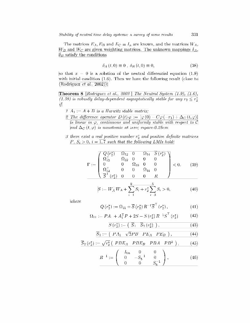


ON THE CONNECTION BETWEEN RICCATI INEQUALITIES AND EQUATIONS IN H ∞ CONTROL PROBLEMS
Adrian Stoica University “Politehnica” of Bucharest, Faculty of Aerospace Engineering Str. Splaiul Independentei No. 313, RO-77226 Bucharest, Romania e-mail: [email protected]
Abstract The paper presents some connections between the solvability conditions expressed in terms of linear matrix inequalities and the ones using Riccati equations. It is shown that the methodology based on the Bounded Real Lemma, mainly used in the singular H ∞ control theory, can be successfully employed in nonsingular problems, providing solvability conditions in terms of the stabilizing solutions to algebraic Riccati equations.
Keywords: H ∞ control, linear matrix inequalities, Riccati equations, Bounded Real Lemma, stabilizing solutions.
1. Introduction
The H ∞ theory captured a major interest in control engineering and in applied mathematics over the last two and half decades. This interest is determined by the fact that the H ∞ optimization provides elegant solutions for many practical problems. Robust control, tracking, filtering, fault detection and identification are only some of the most known areas of applications. From an historical perspective, there were several directions in which the study of this problem has been orientated. Among them one can mention the methods based on operator theory and interpolation, mostly used in the early period (Adamjan et al., 1978), (Ball and Helton, 1983), reduction to Nehari problems (Francis, 1986), polynomial approaches (Kwakernaak, 1986). A major contribution is brought by the

ADVANCES IN AUTOMATIC CONTROL 352
state-space results derived in (Glover and Doyle, 1988), (Doyle et al., 1989) providing necessary and sufficient solvability conditions for the so-called nonsingular H ∞ control problem. These conditions are expressed in terms of the stabilizing solutions of some game-theoretic algebraic Riccati equations (ARE). Explicit formulae and parameterization of the set of all solutions have been also obtained. State-space solutions for the nonsingular H ∞ control problem are also derived by a different technique using the generalized Popov-Yakubovich theory in (Ionescu et al., 1999), (Ionescu and Stoica, 1999). The singular H ∞ control problem arises from the nonsingular case by removing some assumptions. The approaches develop in (Gahinet and Apkarian, 1994), (Boyd et al., 1994), (Iwasaki and Skelton, 1994) use a different methodology, based on the Bounded Real Lemma in inequality form. In this case the solvability conditions are expressed in terms of the feasibility of some specific linear matrix inequalities (LMI). In contrast with the nonsingular H ∞ control problem where the solvability conditions and the solution are derived starting from some particular problems fully exploiting the nonsingularity assumptions, in the singular case the developments are easily performed directly for the general case. Although efficient numerical algorithms to determine the solutions of the corresponding LMI have been developed, there are applications when ill conditioned numerical computations and instabilities occur (see e.g. (Gahinet and Apkarian, 1994)). In such cases it is preferable to replace, if possible, the conditions based on Riccati inequalities by Riccati equations for which several alternative algorithms to compute their stabilizing solutions are available. The aim of this paper is to present some connections between the solvability conditions expressed in terms of LMI and the ones using ARE. It is shown that the general methodology based on the Bounded Real Lemma, mainly used in the singular H ∞ control theory, can be successfully employed in nonsingular problems, providing solvability conditions in terms of the stabilizing solutions to ARE.
2. Problem formulation and preliminary results Consider the generalized two-input, two-output system T with the state space equations:
( ) ( ) ( ) ( )( ) ( ) ( ) ( )( ) ( ) ( )
1 1 2 2
1 1 11 1 12 2
2 2 21 1 ,
x t Ax t B u t B u t
y t C x t D u t D u t
y t C x t D u t
⋅= + +
= + +
= +
(1)
where ( ) nx t ∈R is the state vector, 11 ( ) mu t ∈R is the external input vector,

On the connection between Riccati inequalities and equations in H ∞ 353
22 ( ) mu t ∈R denotes the control variable, 1
1 ( ) py t ∈R includes the regulated output variables and ( ) 2
2py t ∈R is the measured outputs vector. Then, the
H ∞ control problem consists in finding a controller K such that the resulting system obtained by (1) taking 2 2u Ky= is internally stable and
1 1u yT∞< γ , where 0γ > is a given level of attenuation.
1 1y uT denotes the
transfer function from 1u to 1y of the resulting system and the H ∞ norm of a stable system with the transfer function G(s) is defined as
( ) ( )1/ 2maxsup ( ) ( )TG s G j G j−∞<ω<∞∞
= λ − ω ω , max ( )λ ⋅ denoting the
maximal eigenvalue of ( )⋅ . In the following, two preliminary results are stated. The first one is also known as the Bounded Real Lemma and an early proof of it is given in (Anderson and Vongpanitlerd, 1973).
Lemma 1 (Bounded Real Lemma) Let ( ) ( ): , , ,H s A B C D= be a stable system with , ,n n n m p nA B C× × ×∈ ∈ ∈R R R and p mD ×∈R . Then the following assertions are equivalent: i) ( )H s
∞< γ ;
ii) There exists 0X > such that:
T T
T T 0 ;m
m
A X XA XB CB X I D
C D I
+ −γ < −γ
iii) 2 T 0mI D Dγ − > and the Riccati equation
( )( ) ( )1T T 2 T T T T 0mA X XA XB C D I D D B X D C C C−
+ + + γ − + + =
has a stabilizing solution.
Based on the above result, the following theorem providing necessary and sufficient solvability conditions to the H ∞ control problem is proved in (Gahinet and Apkarian, 1994):
Theorem 1 Consider the generalized system (1) and a scalar 0γ > . Then the following assertions are equivalent: i) It exists an kn -order controller such that the resulting system
1 1u yT is
stable and 1 1u yT
∞< γ ;
ii) There exist the symmetric matrices , , ,n nR S R > 0 S 0×∈ >R , such that:

ADVANCES IN AUTOMATIC CONTROL 354
1
1 11
11 1 1 11
12 1 11 12
1 11
0 00 0 0
0
T TT
p
T Tm mm
AR RA RC BC R I D
I 0 IB D - I
+ −γ < γ
N N
N N (2)
1
1 11
1 121 21
22 1 11 22
1 11
0 00 0 0
0 0
T TT
T Tm
p pp
A S SA SB C
B S I DI IC D - I
+
−γ < γ
N N
N N (3)
0, rank ,n nk
n n
R I R In n
I S I S
≥ ≤ +
(4)
where 11
12
N
N and 21
22
N
N denotes bases of the null spaces of the matrices
2 12T TB D
and [ ]2 21C D , respectively.
A crucial role for the further developments is played by the next proposition which proof can be found for example in (Gahinet, 1992):
Proposition 1 If the pair ( ),C A where ,n n p nA C× ×∈ ∈R R has no imaginary unobservable modes then the following assertions are equivalent: i) The Riccati type inequality 0T TAR RA RC CR Q+ + + < (5)
with 1 1 2 2T T n nQ B B B B ×= − ∈R symmetric has a symmetric matrix solution
ˆ 0R > ; ii) The Riccati equation
0T TA X XA XQX C C+ + + = (6)
has a stabilizing solution X . If the conditions i) or ii) are accomplished then 1ˆ0 X R−≤ < .
3. The nonsingular H ∞ control problem In this section it is shown that the solvability conditions in the nonsingular H ∞ case expressed in terms of Riccati equations can be directly recovered via Proposition 1 by the general result stated in Theorem 1.
Theorem 2 Assume that the following conditions hold: A1) 12 12 2
Trank D D m= and 21 21 2Trank D D p= ;

On the connection between Riccati inequalities and equations in H ∞ 355
A2) The system ( )2 1 12, , ,A B C D has no invariant zero on the imaginary axis, that is:
22
1 12rank ,nA j I B
n mC D− ω
= + ∀ω∈
R .
A3) The system ( )1 2 21, , ,A B C D has no invariant zero on the imaginary axis, that is:
12
2 21rank ,nA j I B
n pC D− ω
= + ∀ω∈
R.
Then the H ∞ control problem has an n -order solution if and only if:
1 1
2 211 11 11 11
ˆ ˆ T Tp mI D D and I D Dγ > γ > (7)
and the game-theoretic Riccati equations:
( ) ( )
( ) ( )1 1
1 1
1 12 2
1 11 11 11 1 1 11 11 11 1
1 12 2
1 11 11 1 2 2 1 11 11 1
ˆ ˆ ˆ ˆˆ ˆ ˆ ˆ ˆ ˆ ˆ ˆ
ˆ ˆˆ ˆ ˆ ˆ ˆ ˆ ˆ ˆ 0
TT T T T
p p
T T T T T2p p
A B D I D D C X A B D I D D C X
X B I D D B B B X C I D D C
− −
− −
+ γ − + + γ − + γ − − + γ γ − =
(8)
( ) ( )
( ) ( )1 1
1 1
1 12 2
1 11 11 11 1 1 11 11 11 1
1 12 2
1 11 11 1 2 2 1 11 11 1 0
T T T Tm m
T T T T T2m m
A B D I D D C Y A B D I D D C Y
Y C I D D C C C Y B I D D B
− −
− −
+ γ − + + γ − + γ − − + γ γ − =
(9)
have the stabilizing solutions 0X ≥ and 0Y ≥ respectively, satisfying the condition:
( ) 2 ,XYρ < γ (10)
where ( )ρ ⋅ denotes the spectral radius of ( )⋅ and:
( ) ( )
( )( )
1 1
1
1
2 12 1 1 1 2 12 11 2 12
1 12 12 1 11 12 12 11
1 21 2 1 1 21 21
1 1 11 21 2 2 21 11 11 21 21
ˆ ˆ ˆ: , : , :ˆ ˆ: , : ,
: , : ,
: , : , : .
2
p p
m
2 m
A A B D C B B B D D B B D
C I D D C D I D D D
A A B D C B B I D D
C C D D C C D C D D I D D
+ + +
+ +
+ +
+ + +
= − = − =
= − = −
= − = −
= − = = −
(11)

ADVANCES IN AUTOMATIC CONTROL 356
Proof. The proof is based on Proposition 1 and on Theorem 1. Thus, Theorem 1 shows that the general H ∞ problem has a solution if and only if conditions (2)-(4) hold. In the particular case of the nonsingular H ∞ problem studied in this section, a basis of the null space of the matrix
2 12T TB D
is given by:
11
12 12 2 12
0,n
T T
I
D B U+
= −
N
N (12)
where 12U denotes a basis of the null space of 12TD , that is 12 12 0TD U = .
Then the inequality (2) yields:
( )( )
1
2 2 1 2 12 1
12 1 12 12 11
1 12
ˆ ˆ ˆ ˆ ˆ ˆ
0ˆ
T T T
T T T T2 12
T T11 m
AR RA B B RC B U B
U C R B - U U U D
B D U I
+ − γ + γ + γ γ < −γ
(13)
with 0R > . Further two properties of the matrix 12U are further presented. According with the Singular Value Decomposition Theorem, it exists a unitary matrix 1 1p pU ×∈R such that
( )1 2 2
12 0 p m m
ΣD U
− ×
=
, (14)
where, by virtue of assumption A1, Σ is nonsingular. Thus it results that:
( )2 1 2
112 0 T
m p mD Σ U+ −× −
= (15)
and
1 2
12
0.
p mU U
I −
=
(16)
Taking into account that U is unitary, by the above equation it follows that
1 212 12
Tp mU U I −= (17)
and
12 12 12 12 .TU U I D D += − (18)
On the other hand, by (13) one deduces that

On the connection between Riccati inequalities and equations in H ∞ 357
1
12 12 12 11
11 12
0.T T
Tm
U U U D
D U I
−γ <
−γ
Writing the Schur complement of the element (1,1) and taking into account (17) and (18), from the above inequality one obtains:
( )1 1
111 12 12 11 0.T +
m pI D I D D D−−γ + γ − <
Based on the general properties of the pseudo-inverse one deduces that
( ) ( )1 1 112 12 12 12 12 12
T+ + +p p pI D D I D D I D D− = − − , (19)
which shows that the above inequality is equivalent with the first inequality (7). On the other hand, notice that 2 12
ˆ 0B U = . Using (17) and (18), the Schur complement of the element (2,2) of the matrix in the left side of (13) becomes:
( ) ( )
( ) ( )
1
1
1 1 1
2 2 11 1 12 12 111
1 12 12 1
1 11 11 12 12 1 11 12 12 11
ˆ ˆ ˆˆ
................... .................................. 0.ˆ
T TT +
pT +p
T T + T +p m p
AR RA B BB RC I D D D
RC I D D C R
B D I D D C R I D I D D D
−−
− −
+ − γ + γ − +γ −
<
+ γ − −γ + γ −
Taking into account (19) and the notations (11) one directly obtains that the above inequality is equivalent with:
1
1 12 2 1 1 1 1 11
1 11 11 1 11 11
ˆ ˆ ˆ ˆ ˆˆ ˆ ˆ ˆ0.ˆˆ ˆ ˆ ˆ
T T TT
T T Tm
AR RA B B RC C R B RC D
B D C R I D D
− −
− −
+ − γ + γ + γ <
+ γ −γ + γ (20)
The Schur complement of the element (2,2) of the matrix in the left side of the above inequality has the property:
( ) ( )
( ) ( )1 1
1 1
1 12 2
1 11 11 11 1 1 11 11 11 1
1 12 2
1 11 11 1 1 11 11 1 2 2
ˆ ˆ ˆ ˆˆ ˆ ˆ ˆ ˆ ˆ ˆ ˆ
ˆ ˆˆ ˆ ˆ ˆ ˆ ˆ ˆ ˆ 0.
TT T T T
p p
T T T T Tp p
A B D I D D C R R A B D I D D C
RC I D D C R B I D D B B B
− −
− −
+ γ − + + γ − +γ γ − + γ γ − − <
Denoting 1ˆ :R R−= γ , from the above inequality one obtains that:

ADVANCES IN AUTOMATIC CONTROL 358
( ) ( )
( ) ( )1 1
1 1
1 12 2
1 11 11 11 1 1 11 11 11 1
1 12 2 2
1 11 11 1 1 11 11 1 2 2
ˆ ˆ ˆ ˆˆ ˆ ˆ ˆ ˆ ˆ ˆ ˆ ˆ ˆ
ˆ ˆˆ ˆ ˆ ˆ ˆ ˆ ˆ ˆ ˆ 0.
TT T T T
p p
T T T T Tp p
A B D I D D C R R A B D I D D C
RC I D D C R B I D D B B B
− −
− −
+ γ − + + γ −
+γ γ − + γ − − <
.(21)
In the following one shows that the pair:
( ) ( )1 1
1 12 22
11 11 1 1 11 11 11 1ˆ ˆ ˆˆ ˆ ˆ ˆ ˆ ˆ,T T T
p pI D D C A B D I D D C− −
γ − + γ −
(22)
has no unobservable modes on the imaginary axis. Indeed, assuming that it exists ω∈R such that
( )
( )1
1
1T T21 11 11 11 1
1T2 2
11 11 1
ˆ ˆˆ ˆ ˆ ˆrank ,
ˆˆ ˆ
n p
p
j I A B D I D D Cn
I D D C
−
−
ω − − γ − <
γ −
by the above condition it results that:
( )( )
( )( )
11
11
1 1T T2T T2 2 1 11 11 11 11 11 11 11
11T2 2T2 2 11 11 111 11
1
ˆ ˆˆ ˆ ˆ ˆˆ ˆ ˆ ˆrank
ˆˆ ˆˆ ˆ
ˆrank .
ˆ
n pn p
pp
n
j I A B D I D D CI B D I D D
I D D C0 I D D
j I An
C
−−
−
ω − − γ −γ − γ −γ − ω −
= <
Using the definitions of A and 1C it results that:
( )1
2 12 1
12 12 1
n
p
j I A B D Crank n
I D D C
+
+
ω − + <
−
or equivalently, there exists ,nv v 0∈ ≠R such that
( )1
2 12 1
12 12 1
0.n
p
j I A B D Cv
I D D C
+
+
ω − + = −
On the other hand, from the above equation it follows that:

On the connection between Riccati inequalities and equations in H ∞ 359
2 12 1 2
1 12 12 1 12
0,0
nj I A B D C B v
C D D C D
+
+
− ω + − =
−
that is,
2
2
1 12 12 1
00.
nn
m
Ij I A BC D D C I+
− ω + = −
(23)
Since the vector:
212 1 12 1
0: 0,
0n
m
I vvw
D C I D C v+ +
= = ≠ − −
by (23) it results that
22
1 12rank ,nj I A B
n mC D
− ω + < +
contradicting thus the assumption A2. Therefore the pair (22) has no imaginary unobservable modes and then, applying Proposition 1 for the inequality (21) it follows that the Riccati equation (8) has a stabilizing solution 0X ≥ . The proof of the fact that the Riccati equation (9) has a stabilizing solution is similar and it is based on Proposition 1 together with the assumption A3. On the other hand, by Proposition 1 it also results that
1 1ˆ0 X R R− −≤ < = γ and 1 1ˆ0 Y S S− −≤ < = γ . The first condition (4) in Theorem 2 is equivalent with 0nRS I− ≥ , from which (10) directly follows. The second condition (4) is automatically fulfilled for the case kn n= . The sufficiency part of the theorem simply results by the same steps of the necessity part, in reversed order.
4. A class of H ∞ controllers The result presented in this section is inspired by the paper (Sampei et al., 1990). It gives a strictly proper solution to the H ∞ control problem and it may be applied both in the singular and in the nonsingular case.
Theorem 3 It exists an n -order strictly proper controller H ∞ controller ( ): , , ,0k k kK A B C= if and only if the two following conditions are
accomplished i)
1
211 11 0T
mI D Dγ − > , and

ADVANCES IN AUTOMATIC CONTROL 360
ii) There exist the matrices 2m nF ×∈R and 2n pK ×∈R such that: a) Either the Riccati equations:
( ) 0F X =R (24) and ( ) 0K Y =S , (25)
where
( ) ( ) ( ) ( )
( ) ( ) ( ) ( )1
2 2 1 1 12 11
12
11 11 1 1 12 11 1 12 1 12
: T TF
TT TTm
X A B F X X A B F XB C D F D
I D D XB C D F D C D F C D F−
= + + + + + +
× γ − + + + + +
R
(26)
and
( ) ( ) ( ) ( )
( ) ( ) ( )( )1
2 2 1 1 21 11
12
11 11 1 1 21 11 1 21 1 21
: T T TK
T TT T Tp
Y A KC Y Y A KC YC B KD D
I D D YC B KD D B KD B KD−
= + + + + + +
× γ − + + + + +
S
(27)
have the stabilizing solutions 0X ≥ and 0Y ≥ such that
( ) 2XYρ < γ (28)
or, equivalently b) The Riccati inequalities
( ) 0F X <R (29)
and ( ) 0K Y <S (30)
have the solutions ˆ 0X > and ˆ 0Y > satisfying the condition
( ) 2ˆ ˆXYρ < γ . (31)
Moreover, if the conditions i) and ii) are satisfied then an H ∞ controller has the following realization in terms of the solutions to the Riccati inequalities (29) and (30)
( ) ( )( )
12
2 2
12
ˆ ˆ ˆ
ˆ ˆ
,
2k n
2k n
k
A A B F I YX KC YM
B I YX K
C F
−
−
= + + γ − γ −
= −γ γ −
=
(32)
where

On the connection between Riccati inequalities and equations in H ∞ 361
( )
( ) ( )
( ) ( ) ( )1
2 12 1 12
1
21 1 12 11
1
11 11 1 11 1 12
ˆ:
ˆ ˆ ˆ
ˆ ˆ .
T T
T2n k
T T T2m F
M F B X D C D F
I YX Y B D B FD D
I D D B X D C D F X
−
−
= + + + γ − − +
× γ − + + − R
(33)
Proof. Necessity. The condition i) immediately follows taking into account that
1 1y uT∞< γ implies
( ) ( )1 1 2max ,
T
R R R R R R R RC j I A B D C j I A B D− − λ − ω − + ω − + < γ
∀ ω∈ ∪ ±∞R , from which making ω→∞ , it results that
1
2TR R mD D I< γ . Since 11RD D= , i) directly follows. Further one proves ii).
Assume that it exists a strictly proper controller ( 0kD = ) solving the H ∞ control problem for the generalized system (1). Then according with the Bounded Real Lemma it follows that it exists 0RX > such that:
0Π < , (34) where
( )( )
( )1
12: T T T
R R R R R R R R m R R
T T TR R R R R R
Π A X X A X B C D I D D
B X D C C C
−= + + + γ −
× + + (35)
and
[ ]2 11 12 11
2 21, , , .k
R R R k Rk k k
A B C BA B C C D C D D
B C A B D
= = = =
(36)
Consider the partitions:
1T T; , and ; ,n n n n
R RS N R M
X S S X R RN S M R
−× × = ∈ = ∈
R R . (37)
Without reducing the generality of the reasoning one can consider a solution 0RX > of (34) such that the matrix M introduced above is nonsingular. Indeed, if M is singular one can always consider a small enough perturbation such that M becomes nonsingular, 1
RX − remains positive definite and condition (34) holds. Therefore, in the following it is assumed that M is invertible. Define:

ADVANCES IN AUTOMATIC CONTROL 362
: .0n
R MT
I
=
(38)
Since M invertible, T is invertible, too. Then the inequality (34) is equivalent with:
: 0.TΠ TΠT= < (39)
Performing the partition
11 1211
12 22
: 0, ,n nT
Π ΠΠ Π
Π Π×
= < ∈
R (40)
direct algebraic computations using (35), (36), (38), and the equations obtained from the equality 1
R RX X I− = , give:
( ) ( )
( ) ( )( ) ( ) ( )
1
11 2 2
12
1 1 12 11 11 11
1 11 1 12 1 12 1 12
T
T Tm
TT T
Π R A B F A B F R
B R C D F D I D D
B D C D F R R C D F C D F R
−
= + + +
+ + + γ − × + + + + +
(41)
and
( ) ( ) ( )
( ) ( )1
22 1 21 1 11
12
11 11 1 21 11 1 1 1,
T T
TT T Tm
Π S A KC A KC S S B KD C D
I D D B KD S D C C C−
= + + + + + +
× γ − + + +
(42)
where the following notations have been introduced:
1 1: , : .Tk kF C M R K S NB− −= = (43)
Since 0,Π < it follows that 11 0Π < and 22 0Π < . Further one can write
11Π given by (41) in the equivalent form:
( ) ( )
( ) ( )
( ) ( ) ( )
( )
1
1
1 1
1
12
2 1 11 11 11 1 12
12
2 1 11 11 11 1 12
12
1 12 11 11 11 11 1 12
12
1 11 11 1 0.
T Tm
TT T
m
T T Tp m
T Tm
A B F B I D D D C D F R
R A B F B I D D D C D F
R C D F I D I D D D C D F R
B I D D B
−
−
−
−
+ + γ − +
+ + + γ − + + + + γ − +
+ γ − <
(44)

On the connection between Riccati inequalities and equations in H ∞ 363
Taking into account that 1
211 11 0T
mI D Dγ − > and 0R > , one deduces from (44) that the matrix
( ) ( )1
12
2 1 11 11 11 1 12T T
mA B F B I D D D C D F−
+ + γ − +
is Hurwitz. Then applying Proposition 1 it results that the Riccati equation
( ) ( )
( ) ( )
( ) ( )
( ) ( )
1
1
1
1 1
12
2 1 11 11 11 1 12
12
2 1 11 11 11 1 12
12
1 11 11 1 1 12
12
11 11 11 11 1 12 0
TT T
m
T Tm
TT Tm
T Tp m
A B F B I D D D C D F X
X A B F B I D D D C D F
XB I D D B X C D F
I D I D D D C D F
−
−
−
−
+ + γ − + + + + γ − +
+ γ − + +
× + γ − + =
has a stabilizing solution 10 X R−≤ < . Since the above equation coincides with (24) it follows that this equation has a stabilizing solution 0X ≥ . Further 22Π given by (42) can be written in the equivalent form:
( ) ( )( ) ( )
( ) ( ) ( )
( )( ) ( )
1
1
1
1
12
22 1 21 11 11 11 1
12
1 21 11 11 11 1
12 2
1 21 11 11 11 11 1 21
12
1 21 1 21 1 11 11 1 0
TT T
p
T Tp
TT Tp
T T T2 2p
Π A KC B KD D I D D C S
S A KC B KD D I D D C
S B KD D I D D D B KD S
S B KD B KD S C I D D C
−
−
−−
−−
= + + + γ − + + + + γ −
+ γ + γ − +
+ γ + + + γ γ − < (45)
with 0S > . Applying again Proposition 1 it results that the Riccati equation:
( ) ( )( ) ( )
( )( ) ( ) ( )
1
1
1
1 1
12
1 21 11 11 11 1
12
1 21 11 11 11 1
12
1 11 11 1
12 2
1 21 11 11 11 11 1 21 0
TT T
p
T Tp
T T2p
TT Tm p
A KC B KD D I D D C Y
Y A KC B KD D I D D C
YC I D D C Y
B KD I D I D D D B KD
−
−
−
−−
+ + + γ − + + + + γ −
+ γ γ −
+ γ + + γ − + =

ADVANCES IN AUTOMATIC CONTROL 364
has a stabilizing solution 10 Y S −≤ < . The above Riccati equation can be rewritten as
( ) ( ) ( )
( ) ( )( )( )
1
2 22 2 1 1 21 11
12 2
11 11 1 11 1 21
21 21 1 21 0.
T T T
T T T Tp
T
A KC Y Y A KC YC B KD D
I D D C Y D B D K
B KD B KD
−
−
−
+ + + + γ γ + +
× γ − γ + +
+ γ + + =
Multiplying the above equality by 2γ and denoting : 2Y Y= γ , one directly obtains (25) and thus one concludes that it has the stabilizing solution 0Y ≥ . On the other hand, since 0RX > , it results that 0T
RTX T > . Taking into account again (37), and the equations obtained from the equality
1R R nX X I− = one obtains:
0n
n
R II S
<
, (46)
from which it results 1R S −> or equivalently, 1 1nR S I− − < . Since, as shown
earlier 10 X R−≤ < and 10 : 2Y Y S− −≤ = γ < , the condition (31) in the statement directly follows. The inequalities (29), (30) and (31) follows by pre and post multiplication of (44) and (45) by 1R− and 1S − , respectively. Sufficiency. Consider the nonsingular transform
ˆ0
n n
n
I IT
I
= − (47)
and define
( )
( )2 1 2 1
2 1 2 1
ˆ ˆ ˆ,
ˆ ˆ ˆ ˆR
Y Y XX
Y X Y X
− −
− −
γ − γ − = − γ − γ −
(48)
where ˆ 0X > and ˆ 0Y > satisfy (29), (30) and (31). Then it follows that
1
ˆ ˆˆ ˆ .
ˆ ˆT
R 2
X XTX T
X Y −
−=
− γ
By a Schur complement argument, it results using (31) that ˆ ˆ 0TRTX T >
and therefore 0RX > . Consider now the controller with the state-space realization defined in (32) and (33). Computing ˆ ˆ ˆ: TΠ TΠT= with T defined

On the connection between Riccati inequalities and equations in H ∞ 365
by (47) and with Π having the expression (35), direct algebraic computations give:
( )
( )2 1
ˆ 0ˆ ,
ˆ ˆ ˆ0
F
1F
XΠ
Y Y Y− −
= γ
R
S
Taking into account (29), (30) it follows that ˆ 0Π < and thus 0Π < . Since 0RX > , according with the Bounded Real Lemma it results that the strictly
proper controller ( ), ,k k kA B C is a solution to the H ∞ control problem.
5. Conclusions The theoretical developments in Section 2 show that the well-known solvability conditions for the nonsingular H ∞ control problem can be easily obtained in a general form by Theorem 1 and Proposition 1. For 2
TF B X= − and 2
TK YC= − , (24) and (25) coincide with the Riccati equations derived in (Doyle et al., 1989).
References Adamjan, V.M., D.Z. Arov and M.G. Krein (1978). Infinite block Hankel matrices and related
extension problems. AMS Transl., Vol. 111, 133-156.
Anderson, B.D.O. and S. Vongpanitlerd (1973). Network Analysis. Prentice Hall, Englewood Cliffs.
Ball, J.A. and J.W. Helton (1983). A Beurling-Lax theorem for the Lie group ( ),U m n which contains most classical interpolation theory. J. Op. Theory, Vol. 9, 107-142.
Boyd, S., L. El-Ghaoui, E. Feron and V. Balakrishnan (1994). Linear matrix inequalities in systems and control theory. Studies in Applied Mathematics, SIAM, Philadelphia, PA, Vol. 15.
Doyle, J.C., K. Glover, P. Khargonekar and P. Francis (1989). State-space solutions to standard 2H and H∞ control problem. IEEE-Trans-Autom. Control, Vol. 34, 831-848.
Francis, B.A. (1986). A course in H∞ control theory. Springer Verlag.
Gahinet, P. (1992). A New Representation of H∞ Suboptimal Controllers. Rapport de Recherche, No. 1641, INRIA.
Gahinet, P. and P. Apkarian (1994). A linear matrix inequality approach to H∞ control. International Journal Robust and Nonlinear Control, No. 4, 421-448.

ADVANCES IN AUTOMATIC CONTROL 366
Glover, K. and J.C. Doyle (1988). State-space formulae for all stabilizing controllers that satisfy an H∞ -norm bound and relations to risk sensitivity. Systems & Control Letters, Vol. 11, 167-172.
Ionescu, V., C. Oara and M. Weiss (1999). Generalised Riccati Theory and Robust Control: A Popov Function Approach, John Wiley, 1999.
Ionescu, V. and A. Stoica (1999). Robust Stabilisation and H ∞ Problems. Kluwer Academic Publishers, 1999.
Iwasaki, T. and R.E. Skelton (1994). All controllers for the general H∞ control problem: LMI existence conditions and state pace formulas. Automatica, Vol. 30, 1307-1317.
Kwakernaak, H. (1986). A polynomial approach to minimax frequency domain optimization of multivariable feedback systems, Int. J. Contr., Vol. 44, 117-156.
Sampei, M., T. Mita and M. Nakamichi (1990). An algebraic approach to H∞ output feedback control problems. Systems & Control Letters, Vol. 14, 13-24.

NEW COMPUTATIONAL APPROACH FORTHE DESIGN OF FAULT DETECTION ANDISOLATION FILTERS
A. VargaGerman Aerospace Center,DLR - OberpfaffenhofenInstitute of Robotics and MechatronicsD-82234 Wessling, Germany.E-mail: [email protected]
Abstract We propose a numerically reliable computational approach for the design ofresidual generators for fault detection and isolation filters. The new approach isbased on computing solutions of least dynamical orders of linear equations withrational matrix coefficients in combination with special rational factorizations.The main computational ingredients are the orthogonal reduction of the associ-ated system matrix pencil to a certain Kronecker-like staircase form, the solutionof a minimal dynamic cover design problem, and the computation of stable andproper rational factorizations with diagonal denominators. For all these com-putations we discuss numerically reliable algorithms relying on matrix penciland descriptor system techniques. The proposed residual generator design ap-proach is completely general, is applicable to both continuous- and discrete-timesystems, and can easily handle even unstable and/or improper systems.
Keywords: Fault detection, fault isolation, linear rational equations, rational factorizations,numerical methods.
1. IntroductionIn the model based fault diagnosis, the fault detection task is achieved by
detecting discrepancies between the outputs of the monitored plant and thepredictions obtained with a mathematical model. These discrepancies - calledalso residuals - are indications of faults and are produced by special devicescalled residual generators. From a system theoretic point of view, the resid-ual generators are physically realizable systems having as inputs the measuredoutputs and the control inputs of the monitored system, and as outputs the gen-erated residuals. The residual generators are usually implemented as parts ofcontrol algorithms or as independent monitoring procedures.
367

368 ADVANCES IN AUTOMATIC CONTROL
Several algorithms underlying the design of residual generators require themanipulation of rational matrices. For low dimensional systems, this is pos-sible to some extent by using symbolic manipulation software as provided bytools like Maple or Mathematica. However for large order systems, symboliccomputation is not anymore applicable because of tremendous manipulationefforts, and therefore the use of numerical algorithms is the only possible op-tion. The need to address the numerical issues encountered in designing faultdetection and isolation filters has been already recognized by (3). By usingrecently developed numerically reliable descriptor system algorithms, many ofcomputational problems in the fault detection field can be addressed for highdimensional systems.
We propose a new computational approach for the design of residual gen-erators for fault detection and isolation filters based on solving linear equa-tions with rational matrix coefficients. Additionally, rational factorization tech-niques are employed to ensure the properness and stability of the resultingresidual generators. For the solution of these computational problems we pro-pose numerically reliable algorithms relying on descriptor system techniques.The main computational ingredient in solving linear equations with rationalmatrices is the orthogonal reduction of the associated system matrix pencil toa certain Kronecker-like staircase form. Using this form a solution can be eas-ily constructed, without the need to explicitly invert any rational or polynomialmatrix. To determine stable and proper solutions of least dynamical orders,minimal dynamic cover design techniques in combination with coprime fac-torization procedures are employed. The proposed computational approach todesign residual generators for fault detection and isolation filters is completelygeneral, is applicable to both continuous- and discrete-time systems, and caneasily handle even unstable and/or improper systems. The design procedure ofresidual generators can be easily implemented using the robust numerical toolsavailable in the DESCRIPTOR SYSTEMS Toolbox developed by the author1.
2. Design of fault detection and isolation filtersConsider the linear time-invariant system described by the input-output re-
lations
y(λ) = Gp(λ)u(λ) + Gf (λ)f(λ) + Gd(λ)d(λ), (1)
where y(λ), u(λ), f(λ), and d(λ) are Laplace- or Z-transformed vectors of thep-dimensional system output vector y(t), m-dimensional plant input vectoru(t), q-dimensional fault signal vector f(t), and r-dimensional disturbancevector d(t), respectively, and where Gp(λ), Gf (λ) and Gd(λ) are the transfer-function matrices (TFMs) from the plant inputs to outputs, fault signals tooutputs, and disturbances to outputs, respectively. According to the system

New computational approach for the design of fault detectors 369
type, λ = s in the case of a continuous-time system or λ = z in the case of adiscrete-time system.
The fault detection and isolation (FDI) problem can be formulated as fol-lows: determine a linear residual generator (or detector) of least dynamicalorder having the general form
r(λ) = R(λ)[
y(λ)u(λ)
]
(2)
such that: (i) r(t) = 0 when f(t) = 0; and (ii) ri(t) = 0 when fi(t) = 0, fori = 1, . . . , q. Besides the requirement that the TFM of the detector R(λ) hasleast possible McMillan degree, it is also necessary, for physical realizability,that R(λ) is a proper and stable TFM.
One possibility to determine a least order R(λ) is to solve the followingminimal design problem (18): choose a suitable diagonal M(λ) (i.e., stable,proper and invertible) and find a least McMillan degree solution R(λ) of thelinear equation with rational matrices
R(λ)[
Gf (λ) Gd(λ) Gp(λ)O O Im
]
=[
M(λ) O O]
(3)
which is stable and proper. This equation arises by imposing for a detectorof the general form (2) the condition that r(λ) = M(λ)f(λ) for all d(λ) andu(λ).
To solve the above equation for properly chosen M(λ), the minimum degreealgorithm of (23) can be considered as basis for a possible numerical approachusing polynomial techniques. Alternatively, provided [Gf (λ) Gd(λ) ] is leftinvertible, a numerically reliable inversion based procedure has been proposedby (18). Here we compute first (using a state space based approach) a leastorder left-inverse G+(λ) of
G(λ) =[
Gf (λ) Gd(λ) Gp(λ)O O Im
]
and then determine R(λ) as the numerator of a stable and proper fractionalrepresentation G+
1 (λ) = M(λ)−1R(λ), where G+1 (λ) represents the first q
rows of G+(λ) and M(λ) is diagonal. Note that determining a least orderR(λ) is part of the computation of the left-inverse G+(λ), and can be explicitlyaddressed.
In this paper we propose an alternative approach based on solving the ra-tional equation (3) to obtain a least order stable and proper solution R(λ) bychoosing an appropriate M(λ). This computation can be performed in severalsteps involving manipulation of rational matrices. For each step we proposematrix pencil based reliable numerical algorithms which allow to determine

370 ADVANCES IN AUTOMATIC CONTROL
the solution by computing exclusively with real matrices of state space mod-els. By using the proposed approach, the fault detection and isolation filterdesign problem can be solved in the most general setting. Thus our approachrepresents a completely general solution to the FDI problem, being a numer-ically reliable computational alternative to various inversion based methods(4, 5, 10, 13, 8, 3, 9).
3. Solving rational equationsFor the design of residual generators in the most general setting, we have to
solve a rational equation of the form (3), where we have the additional free-dom of choosing a diagonal M(λ) such that the resulting R(λ) is proper andstable. Since the solution is in general non-unique, we would like to computea solution which has the least McMillan degree.
In order to solve this problem, we consider, for convenience, the more gen-eral dual problem to solve a linear rational system of the form
G(λ)X(λ) = F (λ)M(λ), (4)
where G(λ) and F (λ) are given p × m and p × q rational TFMs, respectively,and we need to choose an invertible diagonal M(λ) such that the resultingsolution X(λ) is proper, stable and has the least possible McMillan degree.It is a well known fact that the system (4) has a solution provided the rankcondition
rank G(λ) = rank [G(λ) F (λ) ] (5)
is fulfilled. We assume throughout the paper that this condition holds.For a given M(λ) the general solution of (4) can be expressed as
X(λ) = X0(λ) + XN (λ)Y (λ),
where X0(λ) is a particular solution of (4) and XN (λ) is a rational basis ma-trix for the right nullspace of G(λ). Thus a straightforward procedure to solve(4) would be to compute first X0(λ) and XN (λ) for M(λ) = I , then to deter-mine a suitable Y (λ) to obtain a solution X(λ) of least McMillan degree, andfinally to choose an appropriate M(λ) ensuring the stability and properness ofX(λ) = X(λ)M(λ).
The main difficulty using this approach is the computation of Y (λ) in thecase when X0(λ) is not proper. In this case the corresponding Y (λ) can beimproper as well and for this computation there is no known computationalprocedure. In contrast, if X0(λ) and XN (λ) are proper rational matrices, thenthe resulting proper Y (λ) can be determined by employing the approach pro-posed by (12) based on minimal cover design techniques. The following con-ceptual procedure is merely a refining of the above steps in order to guarantee

New computational approach for the design of fault detectors 371
the applicability of the approach of (12). For this, we determine M(λ) in a fac-tored form M(λ) = Mf (λ)Ms(λ), where Mf (λ) is a proper and stable factorchosen to ensure the properness of X0(λ) and Ms(λ) is a proper and stablefactor chosen to ensure the stability of the solution X(λ). In what follows weformalize the main steps of the solution procedure and subsequently we dis-cuss suitable computational methods based on pencil manipulation techniquesto perform these steps.
1. Compute a particular solution X0(λ) satisfying G(λ)X0(λ) = F (λ).
2. Compute a proper rational basis XN (λ) of the right nullspace of G(λ).
3. Compute a diagonal Mf (λ) having the least McMillan degree such thatX0(λ) := X0(λ)Mf (λ) is proper.
4. Determine a proper Y (λ), such that the solution
X(λ) = X0(λ) + XN (λ)Y (λ)
has the least possible McMillan degree.
5. Determine a diagonal Ms(λ) having the least McMillan degree such thatX(λ) := X(λ)Ms(λ) is stable.
In what follows we discuss numerically reliable state space computationalalgorithms for each step of the above procedure.
3.1. Computation of X0(λ)
Let assume that the compound TFM [G(λ) F (λ) ] has a minimal descriptorrealization of order n of the form
Eλx(t) = Ax(t) + BGu(t) + BF ν(t)
ξ(t) = Cx(t) + DGu(t) + DF ν(t)(6)
satisfying
[G(λ) F (λ) ] = C(λE − A)−1[BG BF ] + [DG DF ]. (7)
According to the system type, λ also represents here either the differentialoperator λx(t) = x(t) in the case of a continuous-time system or the advanceoperator λx(t) = x(t + 1) in the case of a discrete-time system. Note thatfor most of practical applications [G(λ) F (λ) ] is a proper TFM, thus we canalways choose a realization such that E = I . However, for the sake of gener-ality, we only assume that the pencil A − λE is regular, without assuming Eis nonsingular. In this way, we will also cover the most general case of solvingrational linear systems.

372 ADVANCES IN AUTOMATIC CONTROL
Let SG(λ) and SF (λ) be the system matrix pencils associated to the real-izations of G(λ) and F (λ)
SG(λ) =[
A − λE BG
C DG
]
, SF (λ) =[
A − λE BF
C DF
]
.
Using the straightforward relations[
A − λE BG
O G(λ)
]
=[
In O−C(A − λE)−1 Ip
]
SG(λ)
[A − λE BF
O F (λ)
]
=[
In O−C(A − λE)−1 Ip
]
SF (λ)
it is easy to see that X(λ) is a solution of G(λ)X(λ) = F (λ) if and only if
Y (λ) =[
Y11(λ) Y12(λ)Y21(λ) X(λ)
]
satisfiesSG(λ)Y (λ) = SF (λ). (8)
The existence of the solution of (8) is guaranteed by (5), which is equivalent to
rank SG(λ) = rank [SG(λ) SF (λ) ]. (9)
It follows that instead of solving the rational equation G(λ)X(λ) = F (λ), wecan solve the polynomial equation (8) and take
X(λ) =[
O Im]Y (λ)
[OIq
]
.
In fact, since we are interested in the second block column Y2(λ) of Y (λ), weneed only to solve
[A − λE BG
C DG
]
Y2(λ) =[
BF
DF
]
(10)
and compute X(λ) as
X(λ) =[
O Im]Y2(λ).
The condition (9) for the existence of a solution becomes
rank[
A − λE BG
C DG
]
= rank[
A − λE BG BF
C DG DF
]
. (11)

New computational approach for the design of fault detectors 373
To solve (10), we isolate a full rank part of SG(λ) by reducing it to a par-ticular Kronecker-like form. Let Q and Z be orthogonal matrices to reduceSG(λ) to the Kronecker-like form
SG(λ) := QSG(λ)Z =
Br Ar − λEr Ar,reg − λEr,reg ∗0 0 Areg − λEreg ∗0 0 0 Al − λEl
,
(12)where Areg −λEreg is a regular subpencil, the pair (Ar −λEr, Br) is control-lable with Er nonsingular and the subpencil Al − λEl has full column rank.The above reduction can be computed by employing numerically stable algo-rithms as those proposed in (15, 1).
If Y 2(λ) is a solution of the reduced equation
SG(λ)Y 2(λ) = Q
[BF
DF
]
. (13)
then Y2(λ) = ZY 2(λ) and thus
X(λ) =[
O Im]ZY 2(λ)
is a solution of the equation G(λ)X(λ) = F (λ). Partition
Q
[ −BF
−DF
]
=
B1
B2
B3
in accordance with the row structure of SG(λ). Since Al−λEl has full columnrank, it follows from (11) that B3 = 0. Thus, we can choose Y 2(λ) of the form
Y 2(λ) =
Y 12(λ)Y 22(λ)Y 32(λ)
O
,
where the partitioning of Y 2(λ) corresponds to the column partitioning ofSG(λ). Choosing Y 12(λ) = 0, we obtain
[
Y 22(λ)Y 32(λ)
]
=[
λEr − Ar λEr,reg − Ar,reg
O λEreg − Areg
]−1[
B1
B2
]
.
Let partition [O Im ]Z in accordance with the column structure of SG(λ) as
[O Im ]Z = [Dr Cr Creg Cl ] (14)

374 ADVANCES IN AUTOMATIC CONTROL
and denote
A − λE =[
Ar − λEr Ar,reg − λEr,reg
O Areg − λEreg
]
, B =
[
B1
B2
]
,
C = [Cr Creg ]
Then a particular solution X0(λ) of the equation G(λ)X(λ) = F (λ) can beexpressed in form of a descriptor realization
X0(λ) = C(λE − A)−1B.
To compute X0(λ) we employed exclusively orthogonal similarity transforma-tions. Therefore, this step is numerically stable, because we can easily showthat the computed system matrices in the presence of roundoff errors are exactfor an original problem with slightly perturbed data.
Some properties of X0(λ) can be easily deduced from the computed Kro-necker -like form. The poles of X0(λ) are among the generalized eigenvaluesof the pair (A,E) and are partly fixed, and partly freely assignable. The fixedpoles represent the controllable eigenvalues of the pair (B2, Areg − λEreg).The generalized eigenvalues of the pair (Ar, Er) are called the ”spurious”poles, and they originate from the column singularity of G(λ). These polesare in fact freely assignable by appropriate choice of a (non-orthogonal) righttransformation matrix (18).
If G(λ) and F (λ) have no common zeros then the pair (B2, Areg − λEreg)is controllable. This condition is always fulfilled in the case of solving a sys-tem (4) originating from FDI problems, where F (λ) = [I 0]T is a constantfull column rank matrix. In this case, the solution X0(λ) will be proper if[Gf (λ) Gd(λ) ] (see (1) ) has no infinite zeros (i.e., all infinite eigenvaluesof the matrix pair (Areg, Ereg) are simple). Moreover, a stable and propersolution will exist provided [Gf (λ) Gd(λ) ] is additionally minimum-phase.
More generally, the solution X(λ) of G(λ)X(λ) = F (λ) will have no polein γ (finite or infinite) if cγ(G) = cγ([G F ]), where cγ(G) is the contentof G(λ) in γ as defined by (21). Roughly, this is equivalent to say that thepole and zero structures of G(λ) and [G(λ) F (λ)] at γ coincide. For practi-cal computations, this implies that some or all of common zeros of G(λ) and[G(λ) F (λ)] will cancel. This cancellation can be done either explicitly byremoving the uncontrollable eigenvalues of the pair (B2, Areg − λEreg) us-ing orthogonal staircase algorithms (14), or implicitly at the next steps, duringdetermining X0(λ) and X(λ).
Remark 1. In this moment, we can easily determine a stable and proper so-lution of (4) by choosing an invertible diagonal M(λ) such that X(λ) :=X0(λ)M(λ) is stable and proper. The computation of M(λ) can be done using

New computational approach for the design of fault detectors 375
methods discussed in (18). Note however that the resulting solution is usuallynot of least McMillan degree. Therefore, the next steps of the proposed proce-dure address exclusively the least order aspect.
3.2. Computation of XN(λ)
Using the same reduction of SG(λ) to SG(λ) as in (12), a nullspace basisXN (λ) of G(λ) can be computed from a nullspace basis YN (λ) of SG(λ) as
XN (λ) = [O Im ]ZY N (λ)
We can determine Y N (λ) in the form
Y N (λ) =
I(λEr − Ar)−1Br
OO
.
With Cr and Dr defined in (14), we obtain a descriptor realization of XN (λ)as
XN (λ) = Cr(λEr − Ar)−1Br + Dr.
Note that XN (λ) is a proper TFM which has least McMillan degree (19).Moreover, the poles of XN (λ) are freely assignable by appropriately choos-ing the transformation matrices Q and Z to reduce the system pencil SG(λ).
Remark 2. We can express XN (λ) to have the same state, descriptor and
output matrices as X0(λ). If we denote Br =[
Br
O
]
, then XN (λ) can be also
expressed asXN (λ) = C(λE − A)−1Br + Dr (15)
This representation is evidently not minimal, since all generalized eigenvaluesof the pair (Areg, Ereg) are uncontrollable.
3.3. Selecting Mf(λ)
In principle, this computation can be done simply by solving q independentproper right coprime factorization (RCF) problems for the single-input sys-tems corresponding to each of q columns of X0(λ). Assuming X0,i(λ) is thei-th column of X0(λ), we can compute the proper RCF
X0,i(λ) =X0,i(λ)mf,i(λ)
,
where mf,i(λ) and X0,i are both proper and mutually coprime. The resultingscalar transfer-function mf,i(λ) and rational vector X0,i(λ) are the i-th diago-nal element of Mf (λ) and the i-th column of X0(λ), respectively.

376 ADVANCES IN AUTOMATIC CONTROL
The transfer functions mf,i(λ) can be chosen, for example, in the form
mf,i(λ) =1
(λ + α)n∞,i,
where n∞,i is the number of infinity zeros of X0,i(λ) and α is an arbitraryvalue, representing a desired stability degree for the solution. It is possibleto determine n∞,i efficiently from the resulting Kronecker-like form of thesystem pencil SG(λ). We can assume that Areg−λEreg and B2 are partitionedconformably and have the structure
Areg − λEreg =[
Af − λEf Af,∞ − λEf,∞O A∞ − λE∞
]
, B2 =
[
Bf
B∞
]
,
where Af −λEf and A∞−λE∞ contain the finite and infinite invariant zerosof SG(λ). If we denote b∞,i the i-th column of B∞, then n∞,i + 1 is just theorder of the controllable part of the pair (A∞ − λE∞, b∞,i). To compute n∞,i
we can apply the generalized controllability staircase algorithm of (14) to thepair (E∞ − λA∞, b∞,i) (note that A∞ and E∞ are interchanged).
After having determined a minimal state-space realization (AMf−λI,BMf
,CMf
, 0) for Mf (λ), it is necessary to compute a proper descriptor represen-
tation of X0(λ) = X0(λ)Mf (λ). This can be done in two steps: first, re-move all uncontrollable infinite eigenvalues from the state-space realization ofX0(λ)Mf (λ) applying the algorithm of (14) and then remove the non-dynamicpart applying standard techniques (22). Both steps can be performed efficientlyby exploiting the inherited structure of the system matrices of X0(λ) from theKronecker-like structure of SG(λ). Note that in the first step we also eliminatethe uncontrollable infinite eigenvalues originating from the common infinitepoles and zeros of G(λ) and F (λ). We omit further details here because oflack of space.
3.4. Computation of a least order X(λ)
We assume that X0(λ) and XN (λ) are proper TFMs and possess state-spacerepresentations sharing the same descriptor, state and output matrices
[
X0(λ) XN (λ)]
=
[A − λE B Br
C D Dr
]
(16)
with E non-singular. This can be easily achieved by performing all relevanttransformations employed to eliminate the non-proper part of X0(λ)Mf (λ)also on the non-minimal realization (15) of XN (λ).
It was shown by (12) that computing a least order solutionX(λ) = X0(λ)+XN (λ)Y (λ) by choosing an appropriate proper Y (λ) is equivalent to deter-

New computational approach for the design of fault detectors 377
mine a feedback matrix Fr and a feedforward matrix Lr to cancel the maxi-mum number of unobservable and uncontrollable poles of
X(λ) =
[A + BrFr − λE B + BrLr
C + DrFr D + DrLr
]
.
It can be shown that if we start with a minimal realization of [G(λ) F (λ) ],then we can not produce any unobservable poles in X(λ) via state-feedback.Therefore, we only need to determine the matrices Fr and Lr to cancel themaximum number of uncontrollable poles.
(12) has shown that this problem can be solved as a minimal order dynamiccover design problem. Consider the set
J = V : Im B + AV ⊂ Im Br + V,where A := E−1A, B := E−1B, and Br := E−1Br. Let J ∗ denote the setof subspaces in J of least dimension. If V ∈ J∗, then a pair (Fr, Lr) can bedetermined such that
(A + BrFr)V + Im (B + BrLr) ⊂ V.
Thus, determining a minimal dimension V is equivalent to a minimal ordercover design problem, and a conceptual approach to solve it has been indicatedby (12). The outcome of his method is, besides V , the pair (Fr, Lr) whichachieves a maximal order reduction by forcing pole-zero cancellations. Thisapproach has been turned into a numerically reliable procedure by (20). In thisprocedure Fr and Lr are determined from a special controllability staircaseform of the pair (A − λE, [ Br B ]) obtained by using a numerically reliablemethod relying on both orthogonal and non-orthogonal similarity transforma-tions. An additional feature of this procedure is that all uncontrollable eigen-values of the pair (A − λE, B), arising from common poles or zeros of G(λ)and F (λ) are also eliminated.
3.5. Selecting Ms(λ)
The computation of Ms(λ) can be done simply by solving q stable RCFproblems for the single-input systems corresponding to each columnXi(λ) ofX(λ)
Xi(λ) =Xi(λ)ms,i(λ)
.
One distinctive feature of these single-input factorization problems is that eachXi(λ), has generally an uncontrollable descriptor realization. This aspect ishandled automatically when employing the Algorithm GRCF-P of (16). Sinceeach of resulting ms,i(λ) has least McMillan degree, the resulting diagonalmatrix Ms(λ) has least McMillan degree as well.

378 ADVANCES IN AUTOMATIC CONTROL
4. ExamplesExample 1. Consider the following simple continuous-time example taken
from (6):
Gp(s) =
1s + 1
1(s + 1)2
, Gf (s) =
[01
]
, Gd = 0.
A minimal order left-inverse of Gf (s) is Q(s) = [ 0 1 ], which is properand stable. According to (4), a residual generator can be determined in theobserver-like form
r(s) = Q(s)(y(s) − Gp(s)u(s)).
This leads to a second order stable and proper detector
R(s) = Q(s)[ I − Gp(s) ] =[
0 1 − 1(s + 1)2
]
which is however not of least possible order.We apply now the proposed approach to compute a least order detector. For
this simple model we will explicitly manipulate rational matrices instead ofstate space matrices. The TFMs defining the equation (4) are given by
G(s) =
0 1 01
s + 11
(s + 1)21
, F =[
10
]
.
A particular solution X0(s) of the equation G(s)X(s) = F and a rationalnullspace basis XN (s) of G(s) are
X0(s) =
01
− 1(s + 1)2
, XN (s) =
−101
s + 1
.
Note that XT0 (s) is the second order detector determined previously. If we
choose Y (s) =1
s + 1, then we obtain a first order stable and proper detector
R(s) = (X0(s) + XN (s)Y (s))T =[
− 1s + 1
1 0]
having the least possible McMillan degree.

New computational approach for the design of fault detectors 379
Example 2. This example is the descriptor system described in (11) corre-sponding to a linearized three-links planar manipulator model. This model hasstate vector dimension n = 11, command input vector dimension m = 3, faultvector dimension q = 2, no disturbance input, and output vector dimensionp = 4 . This model is not minimal and a minimal realization has order 5 andis proper.
The method proposed by (11) is essentially equivalent to design two inde-pendent FDI filters. By considering the fault input 1 as fault and fault input 2as disturbance, a 4-th order FDI filter R1(s) has been designed by (11). Sim-ilarly, by considering fault input 2 as fault and fault input 1 as disturbance, heobtained a 4-th order FDI filter R2(s). In this way, a FDI filter of order 8 hasbeen determined by stacking the two designed filters
R(s) =[
R1(s)R2(s)
]
.
By using the new approach proposed in this paper we can determine a resid-ual generator which has a least order equal to 2. In the rational system (4) tobe solved G(s) is 5× 7 and F (s) is 5× 2, thus R(s) = XT (s) will be a 2× 7matrix. A particular solution X0(s) has been determined having a state spacerealization of order 10, with the pair (A,E) having 3 finite and 7 infinite gen-eralized eigenvalues. The nullspace basis XN (s) is 7 × 2 and has dynamicalorder 3. With Mf (s) of the form Mf (s) = 1
s+1I2, we can eliminate all infinite
poles of X0(s) and the resulting proper solution X0(s) = X0(s)Mf (s) hasorder 5. After performing the minimum cover design, we get a stable solutionX(s) = X(s) of order 2 with both eigenvalues stable and equal to -1. Forreference purposes we give the resulting 2-nd order FDI filter
R(s) =
−0.01042s + 0.04455s + 1
0.03462s + 1
−0.03899s + 1.936s + 1
1s + 1
s
s + 10
· · ·−0.02753s + 1.377
s + 10
0.03899s + 1
0.02753s + 1
0 − 1s + 1
0 0
.
5. ConclusionsWe proposed numerically reliable approaches to solve several basic com-
putational problems encountered in the design of FDI filters, namely: (1) thesolution of linear rational equations; (2) the computation of rational nullspacebases of rational matrices; (3) the reduction of the dynamical orders of the so-lutions by employing minimal dynamic cover design techniques; and (4) the

380 ADVANCES IN AUTOMATIC CONTROL
computation of stable and proper rational factorizations with diagonal denomi-nators. Each of these computations can be performed using numerically stableor numerically reliable algorithms. Using such algorithms, the FDI problemcan be solved in the most general setting. Our approach provides, for the firsttime, a satisfactory numerical solution to this problem. Note that least orderresidual generator design algorithms have been already proposed to solve thesimpler fault detection problem (i.e., without isolation) by (7) using a polyno-mial basis approach, and by (19) using state space computational techniques.
For the implementation of the proposed residual generator design approach,all necessary basic numerical software is available in the DESCRIPTOR SYS-TEMS Toolbox for MATLAB (17), as for example, the computation of Kro-necker -like staircase forms, computation of standard and special controllabil-ity forms (required in minimum cover design), computation of poles and zerosof descriptor systems, determination of minimal realizations, stable coprimefactorization, etc. The basic computational tools in this toolbox are severalfunctionally rich MEX-functions, representing MATLAB interfaces to power-ful and numerically robust Fortran subroutines partly available in the controland systems library SLICOT (2).
Notes1. http://www.robotic.dlr.de/control/num/desctool.html
References
[1] Beelen, T. and P. Van Dooren (1988). An improved algorithm for the computation ofKronecker’s canonical form of a singular pencil. Lin. Alg. & Appl. 105, 9–65.
[2] Benner, P., V. Mehrmann, V. Sima, S. Van Huffel and A. Varga (1999). SLICOT – asubroutine library in systems and control theory. In: Applied and Computational Control,Signals and Circuits (B. N. Datta, Ed.), Vol. 1., pp. 499–539. Birkhauser.
[3] Chen, J. and R. J. Patton (1999). Robust Model-Based Fault Diagnosis for Dynamic Sys-tems, Kluwer Academic Publishers, London.
[4] Ding, X. and P. M. Frank (1990). Fault detection via factorization. Systems & ControlLett. 14, 431–436.
[5] Frank, P. M. and X. Ding (1994). Frequency domain approach to optimally robust residualgeneration and evaluation for model-based fault diagnosis. Automatica 30, 789–804.
[6] Frisk, E. (2000). Order of residual generators – bounds and algorithms. Prepr. IFAC Symp.SAFEPROCESS’2000, Budapest, Hungary, pp. 599–604.
[7] Frisk, E. and M. Nyberg (2001). A minimal polynomial basis solution to residual gener-ation for fault diagnosis in linear systems. Automatica 37, 1417–1424.
[8] Gertler, J. (1998). Fault Detection and Diagnosis in Engineering Systems, Marcel Dekker,New York.
[9] Gertler, J. (2000). Designing dynamic consistency relation for fault detection and isola-tion. Int. J. Control 73, 720–732.

New computational approach for the design of fault detectors 381
[10] Gertler, J. J. and R. Monajemy (1995). Generating directional residuals with dynamicparity relations. Automatica 31, 627–635.
[11] Hou, M. (2000). Fault detection and isolation for descriptor systems. In: Issues of FaultDyagnosis for Dynamic Systems (R. J. Patton, P. M. Frank and R. N. Clark, Eds.),Springer Verlag, London. pp. 115–144.
[12] Morse, A. S. (1976). Minimal solutions to transfer matrix equations. IEEE Trans. Autom.Control 21, 131–133.
[13] Peng, Y., A. Youssouf, Ph. Arte and M. Kinnaert (1997). A complete procedure for resid-ual generation and evaluation with application to a heat exchanger. IEEE Trans. ControlSystems Technology 5, 542–555.
[14] Varga, A. (1990). Computation of irreducible generalized state-space realizations. Kyber-netika 26, 89–106.
[15] Varga, A. (1996). Computation of Kronecker-like forms of a system pencil: Applications,algorithms and software. Proc. CACSD’96 Symposium, Dearborn, MI, pp. 77–82.
[16] Varga, A. (1998). Computation of coprime factorizations of rational matrices. Lin. Alg.& Appl. 271, 83–115.
[17] Varga, A. (2000). A descriptor systems toolbox for MATLAB. Proc. CACSD’2000 Sym-posium, Anchorage, Alaska.
[18] Varga, A. (2002). Computational issues in fault-detection filter design. Proc. ofCDC’2002, Las Vegas, Nevada.
[19] Varga, A. (2003a). On computing least order fault detectors using rational nullspacebases. Prepr. of IFAC Symp. SAFEPROCESS’2003, Washington D.C.
[20] Varga, A. (2003b). Reliable algorithms for computing minimal dynamic covers.(submitted to CDC’2003).
[21] Verghese, G. and T. Kailath (1981). Rational matrix structure. IEEE Trans. Autom. Con-trol 26, 434–439.
[22] Verghese, G., B. Levy and T. Kailath (1981). A generalized state-space for singular sys-tems. IEEE Trans. Autom. Control 26, 811–831.
[23] Wang, S.-H. and E. J. Davison (1973). A minimization algorithm for the design of linearmultivariable systems. IEEE Trans. Autom. Control 18, 220–225.


SETTING UP THE REFERENCE INPUT IN SLIDING MOTION CONTROL AND ITS CLOSED-LOOP TRACKING PERFORMANCE
Mihail Voicu and Octavian Pastravanu Department of Automatic Control and Industrial Informatics Technical University “Gh. Asachi” of Iaşi Blvd. Mangeron 53A, 700050 Iaşi, Romania, Phone / Fax: 40-232-230751 e-mail: [email protected], [email protected]
Abstract On the background of the design of sliding motion controller based on flow – invariance method, the paper presents a solution for setting up the reference input. It uses a state transformation which contains, as a component of the new state vector, the error between the reference input v(t) and the plant output y(t). It is shown that the feedback sliding mode controller ensures the closed-loop tracking performance y(t) = v(t) = VsinΩt under certain conditions in the amplitude – frequency domain (V, Ω).
Keywords: reference input, feedback control, sliding motion control, flow – invariance method, tracking performance
1. Introduction In this paper, based on two necessary and sufficient conditions, obtained via flow – invariance method, which allow a unified design of the sliding domain reaching and sliding motion, one approaches the problem of setting up the reference input. Some preliminaries on sliding motion control and the necessary and sufficient conditions for sliding motion and for sliding domain reaching are presented in section 2. In section 3 one presents a solution for setting up the reference input which takes the natural advantage of the feedback control explicitly and directly dependent on the error between the reference input and the plant output. Some concluding remarks are formulated in section 3.

ADVANCES IN AUTOMATIC CONTROL 384
2. Reaching and sliding motion control Consider the linear time – invariant system:
n qu ,t , ,u ,.
+= + + ∈ ∈ ∈ ∈R R R Rx Ax b Dz x z , (1)
,y y= ∈ Rhx , (2)
where x is the state (completely and directly available for measurement), u and y are the scalar control and output respectively, and z is a disturbing input; : ( ), : ( ), : ( )ij j ija b d= = =A b D and )(: jh=h are constant matrices of appropriate dimensions. Let us associate with system (1), (2) the following switching hyperplane:
: ; 0n TS s= ∈ = =Rx c x , (3)
where [ ]1: Tnc c= …c , with 1nc = , is a constant vector and T)(
symbolizes the transposition. Defining the state transformation from [ ]1 1: T
n nx x x−=x to
[ ]1 1T
nx x s−= …x , with Ts = c x , by:
1
( )
0, : 1
nTn
− = =
Ix Px P c , (4)
where In–1 is the unit matrix of order n–1, and c(n) denotes the vector obtained by deleting the n-th element of c, system (1), (2) becomes:
( ) ( ) ( ) ( ) ( )n
n n n n nu z= + + +x Ex a s b D , (5)
( ) ( ) ( ) ,T n T T n T Tn n n u = − + + + s c A a c x c a s c b c Dz (6)
xhP ~1−=y . (7)
In (5) – (7) ( )ij in j: a a c= −E is an ( 1) ( 1)n n− × − matrix, A(n) and D(n) denote the matrices obtained by deleting the n – th row and column of A and D respectively, an is the n-th column of A; ( ) ( ), n
n nx a and ( )nb denote the vectors obtained by deleting the n-the component of x, an and b, respectively. The achievement of sliding motion of x on S towards an equilibrium point in S⊂Rn consists in the synthesis of control ( , )u t x , discontinuous on

Setting-up the reference input in sliding motion control 385
S, such that the following three requirements are fulfilled:
1. For every initial pair )\(),( 00 St nRR ×∈ +x , with 00 )( xx =t , system (1) evolves towards S, i.e. its state reaches hyperplane S, in a reaching point, after a finite time interval 00 ],,[ tt >ττ . This is the reaching condition.
2. Since the reaching instant τ, corresponding to the reaching point, the state of system (1), (2) remains to evolve on S. This evolution is called the ideal sliding motion and S is the ideal sliding domain for system (1), (2). This is the ideal sliding motion condition.
3. The ideal sliding motion (on S) must be asymptotically stable towards an equilibrium point (usually or conventionally 0~ == xx ) belonging to S. (Subsidiary and implicitly the disturbance rejection is (eventually) desirable.) This is the stability condition of the ideal sliding motion.
Chronologically (i.e. in the dynamics of system (1), (2)), conditions 1o and 2o must be successively fulfilled, while 2o and 3o must be simultaneously satisfied. This means that for each pair (t0, x0)∈R+×(Rn \ S) the whole evolution of system (1), (2) covers two concatenated time intervals: first, a finite one, [t0, τ], according to condition 1o, followed by the second one, (τ, tf), finite or not, according to conditions 2o and 3o. This essential and, as a matter of fact, natural concatenation of the reaching process followed by the ideal sliding motion has been approached in a unified manner by Voicu and Moroşan (1989; 1991; 1997), Moroşan and Voicu (1994), and Moroşan (1994) using the flow – invariance method, see (Voicu, 1984a; 1984b; 1987; Voicu and Pastravanu, 2003). According to (Voicu and Moroşan, 1997), the starting point of this approach was formalized by Definition 1 (pertaining to the ideal sliding domain) and correspondingly characterized by Theorem 4 (based on the flow – invariance method), and, via the flow structure of the state space induced by sliding motion control (unfolded by Theorem 1), by Theorem 5 which characterizes the reaching process as a natural flowing precursor of the ideal sliding motion. In view of Definition 1 and Theorems 4 and 5 (Voicu and Moroşan, 1997) it follows that for the control design only equation (6) rewritten in the following equivalent form is to be used:
1
1
( )n
T i n T n T Ti i
i
s c x s u−
=
= − + + +∑c a a c a c b c Dz , (8)
where ai is the i-th column of A. Taking into account the possibility that cT(ai – ci an) = 0 for some i, let us define the index sets:
1, 2, ..., 1 , ; ( ) 0T i niI n J i I c c= − = ∈ − ≠a a . (9)

ADVANCES IN AUTOMATIC CONTROL 386
For cTb ≠ 0, one can synthesize the following control algorithm:
( ) ( )( ) ( ) ( )r s n z nu u s u u= − − −x x , (10)
where
0
0
, 0,( ) , 0, 0,
, 0,r r r
su s s s
s
<= + = =− >
δρ δ δ
δ (11)
has to control the reaching process;
( ), 0,
( ) ,, 0,
i is n i i i
i ii J
x su x
x s∈
<= Ψ Ψ = >
∑xβα
(12)
is the sliding motion control;
0( )
0
, 0,( )
, 0,z ns
us
<= >
xβα
(13)
ensures the disturbance rejection. Clearly, ρ, δ0,αi, β i (i ∈ J) and α 0, β0 are the design parameters of the variable structure controller which are to be adjusted in order to fulfill the requirements 1o – 3o. Using inequalities (15) and (16) of Theorem 4 (Voicu and Moroşan, 1997), for equation (8) the following result can be formulated.
Theorem 1 Hyperplane S is the ideal sliding domain for system (1) – (4), (10) – (13), with cTb ≠ 0, if and only if
( )( ), ,
T T i ni i
T T i ni i
αi J
≥ −
≤ − ∈
c b c a c ac b c a c aβ
(14)
0
0
sup ( )
inf ( ).
T T
tT T
t
t
t
≥
≤
c b c Dz
c b c Dz
α
β (15)
In order to characterize the reaching process as a precursor of the sliding motion, let us introduce the following reaching function:
0( )
0 0(| | ) sgn( ), [ , ],( )
0 , ( , ),
t t
f
s e s t tr t
t t
− − + − ∈ = ∈
λδ δ τ
τ (16)
where s0 = : s(x0) = s(x(t0)), and δ > 0, λ > 0, τ > t0 are pre-assignable

Setting-up the reference input in sliding motion control 387
parameters. It is easy to verify that the reaching function (16) satisfies the statements 1o and 2o of Theorem 5 (Voicu and Moroşan, 1997), with
( ) 001
0 ||1ln tst >++= − δλτ (τ being the reaching instant, i.e. r(τ) = 0). Using the statement 3 of Theorem 5 (loc cit) with (11) – 13), under (14), (15), one can formulate the following result.
Theorem 2 For each pair (t0, x0)∈R+×(Rn \ S) the state of system (1) – (4), (10) – (13), with cTb ≠ 0, reaches ideal sliding domain S if and only if
0 .
T T n
T T n
≥ +
≤
c b c ac b c a
ρ λδ
(17)
Equations (10) – (13) and inequalities (14), (15) and (17) define the (variable) structure and the adjustable parameters of the controller according to requirements 1o and 2o. Using the equivalent control method (Utkin, 1978), i.e. by solving the equation: 0s = (18)
(according to (6)) with respect to u and replacing the result, with s = 0, into (5), one obtains the ideal sliding equations:
1 1( ) ( ) ,n n= +x A x D z (19)
0s = (20)
where matrices A1 and D1 can be appropriately calculated. If rank rank [ ],=b b, D (21)
then (Utkin, 1978) 1 0=D (22)
and the disturbance rejection is ensured. The stability of system (19) depends on A1 only and may be improved (according to requirement 3o) by an additional state/output feedback in (10). Under these circumstances the state (and output) trajectories of system (1) – (4), (10) – (13) evolve with pre-assignable velocity (for the state only) from each initial state x0
∈ Rn \ S towards ideal sliding domain S and then towards the final equilibrium point 0~ == xx (and y = 0 respectively).
3. Setting up the reference input The problem of setting up the reference input in the control (variable) structure with a sliding motion controller may be solved in the following two manners.

ADVANCES IN AUTOMATIC CONTROL 388
The first solution, presented and analyzed by Utkin (1978), consists in the introduction of an additional term in equation (10), depending on the scalar reference input v. This means that (10) has to be replaced by:
,v cu u u= + (23)
where vu vα= (24)
is the reference input term with α = constant, and ( ) ( )( ) ( ) ( )c r s n z nu u s u u= − − −x x (25)
is the reaching, sliding motion and rejection control. Because output y should track reference input v, coefficient α is to be chosen, e.g. pertaining to the steady state of the whole system, such that: ss ssy v= (26)
(subscript ss denotes the steady state), i.e.
0det,)( 11 ≠−= −− AbhAα . (27)
Unlike this solution, the second one, which is addressed in the sequel, takes the natural (and classical) advantage of the feedback control explicitly and directly dependent on the error between reference input v and plant output y, i.e. (for instance):
1 :x v y= − . (28)
In order to expose this solution, let us consider the plant:
qn utu RRRR ∈∈∈∈++= + zxzDbxAx ,,,, (29)
y = hx , (30)
where x is the state (completely and directly available for measurement), and , ,A b D and h are time – invariant matrices of appropriate dimensions. The trivial case 1: 0nh h = = …h being excluded, for the sake of
simplicity, let us suppose that:
1 0h ≠ (31) (as it was subsidiary assumed by (28)). In this case, error (28), with (30), may be taken into consideration, for instance, by the transformation:
1v= −x i Qx (32)

Setting-up the reference input in sliding motion control 389
where
1 (1)
1: ,
0 n
h
−
=
hQ
I (33)
i1 is the first column of In and (1)h is obtained by deleting the first element of
row matrix h . Using the transformation (32) with (33) for the plant described by (29) and (30), one obtains:
u= + + +x Ax b Dz Fw , (34)
y v= +hx , (35)
where
[ ]
1
1 1
: , : , ,
: , , : 1 0 0
−= = − = −
= − = − …A QAQ b Qb D QDF a i h
(36)
[ ] 2: Tv v= ∈ Rw . (37)
In comparison with equation (1), equation (36) contains the disturbing term Fw and, in control equation (10) the term uz has to be replaced with uzw accordingly. Under these circumstances Theorem 1 must be adequately completed as follows.
Theorem 3 Hyperplane S is the ideal sliding domain for system (34), (35), (3), (4), (10) – (13), with cTb ≠ 0, if and only if (14), (15) are met and
0
0
sup ( )
inf ( )
T T
tT T
t
t
t
≥
≤
c b c Fw
c b c Fw
α
β. (38)
At the same time, for the reaching function (16), Theorem 2 is to be applied to system (34), (35), (3), (4), (10) – (13). According to (19) and (20), the ideal sliding equations are now:
1 1 1( ) ( )n n= + +x A x D z F w , (39)
0s = , (40)
where matrices A1, D1 and F1can be appropriately calculated. In addition to (21), (22), one has to point out that if
rank rank [ , ]=b b F (41)

ADVANCES IN AUTOMATIC CONTROL 390
then
1 0=F (42)
and the rejection of disturbance w is also ensured. Clearly, related to the steady state of the whole system, one may assert that if A1 is Hurwitzian, then 0= =x x , together with (32), (33), as a final result of the control (10), yield the steady state (26) as a natural consequence of the feedback control explicitly and directly dependent on the error between v and y. Moreover, for any w (see (37)) satisfying conditions (38), the system (34), (35), (3), (4), (10) – (13), after a settling time depending on x0, λ and δ (from (16)) and the greatest real part of the eigenvalues of Hurwitzian matrix A1, achieves the closed-loop tracking performance:
( ) ( )y t v t= . (43)
4. Closed-loop tracking performance The employment of (15) and (38) pertaining to the choice of parameters α0 and β0 demands some knowledge about disturbance z and reference input v (see (37)). In order to illustrate the tracking performance of the closed-loop system and, correspondingly, to determine the tracking conditions in the amplitude – frequency domain, let us consider that the system is not disturbed by z, i.e. z = 0, and the reference input has the following form:
v(t) = VsinΩt. (44)
Using (44) in (38), with (36), (37), and by assuming that cTb > 0 and 000 >−= βα , one successively obtains:
),cossin(sup 11
00 ΩtΩctΩV T
t
TT +−≥−= acbcbc βα
( ) ( ) .2/1
21
2100
+≥−= ΩcV TTT acbcbc βα (45)
Tacking into account that usually
max000 αβα ≤−=< , (46)
where maxα depends on some technological limits (saturation, limited control power) characterizing the plant (30), from (45) and (46) one obtains for the closed-loop tracking performance (43) the following admissible amplitude – frequency domain:

Setting-up the reference input in sliding motion control 391
( ) ( ) ( ) ( ) ,2/1
21
21max
2/12
121
0
−−
+≤
+≤ ΩcΩcV TTTT acbcacbc αα (47)
which is ensured by the feedback control explicitly and directly dependent on the error (28) between reference input v and plant output y. Finally, let us remark that suitable transformations such as (32), which include the input – output error (28) and some other errors pertaining to the velocity, acceleration etc, may be taken into consideration in order to improve the tracking behavior of the feedback control systems with sliding motion controller.
5. Concluding remarks In this paper, on the background of two necessary and sufficient conditions, obtained via flow – invariance method, which allow a unified design of the (variable structure) state feedback controller ensuring the sliding – domain reaching and the sliding motion, one gives a solution for setting-up the reference input for the whole system containing a variable structure controller. Unlike the usual solution (which consists in an additional term dependent on the reference input, in the plant control), the solution presented in the paper uses a state transformation (e.g. (32), (33)) which contains, as a component of the new state vector, the error between the reference input v and the plant output y. Under these circumstances the feedback controller based on this new state vector, under certain conditions and after an inherent settling time, ensures the closed-loop tracking performance ( ) ( )y t v t= .
References Moroşan, B.I. (1994). Digital Variable – Structure Systems Studied by Flow – Invariance
Method. Doctoral thesis (in Romanian), Technical University of Iaşi.
Moroşan, B.I., Voicu, M. (1994). General sliding mode systems analysis and design via flow – invariance method. Studies in Informatics and Control, vol. 3, 4, pp. 347 – 366.
Utkin, V.I. (1978). Sliding Modes and Their Application in Variable Structure Systems. MIR, Moscow.
Voicu, M. (1984a). Free response characterization via flow – invariance. 9-th World Congress of IFAC, Budapest. Preprints, vol. 5, pp. 12 – 17.
Voicu, M. (1984b). Componentwise asymptotic stability of linear constant dynamical systems. IEEE Trans. on AC, AC – 29, 10, pp. 937 – 939.
Voicu, M. (1987). On the application of the flow – invariance method in control theory and design. 10 – th World Congress of IFAC, Munich. Preprints, vol. 8, pp. 364 – 369.
Voicu, M., Moroşan, B.I. (1989). State space flow structure induced by sliding motion control. Bul. Inst. Politehnic din Iaşi, III, t. XXXV (XXXIX), 3 – 4, pp. 25 – 29.

ADVANCES IN AUTOMATIC CONTROL 392
Voicu, M., Moroşan, B.I. (1991). Variable – structure controller for feedback positioning of d.c. electric motor. Rev Roum. Sci. Techn., ser. Electrot. Energet., t. 36, 2, pp. 247 – 264.
Voicu, M., Moroşan, B.I. (1997). Variable – structure control characterization and design via flow – invariance method. Int. J. Automation Austria, Jg. 5, 1, pp. 12 - 24.
Voicu M., Pastravanu O. (2003). Flow-invariance method in control – a survey of some results. In Voicu M. (Ed.), Advances in Automatic Control, Kluwer, pp. 393 - 434 (in this volume).

FLOW-INVARIANCE METHODIN CONTROL - A SURVEY OFSOME RESULTS
Mihail Voicu and Octavian PăstrăvanuDepartment of Automatic Control and Industrial Informatics
Technical University of Iasi
Blvd. D. Mangeron 53A, RO-700050 Iasi, Romania
E-mail: mvoicu,[email protected]
Abstract This paper represents a survey of the main contributions of the twoauthors to the application of the flow-invariance method in control sys-tem analysis and design. By considering time-dependent state hyper-intervals, a componentwise approach has been developed for the evalua-tion of the behaviour of continuous-time dynamical systems, in general,and of their stability (regarded as a free response) in particular. Thus, aspecial type of asymptotic stability, called componentwise (exponential)asymptotic stability was introduced, which allows individual monitoringof each state variable, unlike the standard concept of asymptotic sta-bility offering a global characterisation in terms of vector norms. Con-sequently, new and refined instruments were created for the analysisof linear and nonlinear dynamical systems, with constant or intervaltype coefficients. These instruments are equally useful in synthesis fordealing with componentwise stabilizability and detectability. The sameframework constructed on the flow-invariance background is also able toaccommodate the design of the sliding motion control. The paper doesnot contain proofs for the enounced results in order to keep the size ofthe text under some moderate limits, but these proofs can be found inthe cited references.
Keywords: control systems, time dependent flow-invariance, componentwise asymp-totic (exponential) stability, componentwise absolute stability, robust-ness, interval matrix systems, nonlinear uncertain systems, componen-twise detectability and stabilizability, sliding motion control
1. IntroductionGenerally speaking, the object of flow-invariance theory is the “stream”,in the state space X of a dynamical system (described by a differentialequation), of state trajectories x(t), 0 0[ , ],f ft t t t t , starting in the
initial states 0 0( )x t x X and arriving in the corresponding current
states ( )x t X . More precisely, the evolution operator :t X X ,

394 ADVANCES IN AUTOMATIC CONTROL
which generates the flow of Σ, is the application that transforms the(set of) initial states into (the set) of current states and, under certainassumptions and details, Σ itself can be represented by x(t) = Φt(x0).As expected, the notion of flow and the entire conceptual vision aroundit, based on the investigations of Φt and by means of Φt, offer morerefined instruments for the qualitative analysis of differential equationsthat may unfold more subtle structural properties and characterizationsof dynamical systems. In this respect the classical attributive (joint)concept of invariance opened a special field of research that studies theexistence and characterizations of some (nonempty) flow-invariant sub-setsXi ⊆ X (not necessarily time-invariant) having the property that foreach x0 ∈ Xi system Σ fulfils x(t) ∈ Xi for each t ∈ [t0, tf ]. It is worthto be noticed here that such behaviour, interesting by itself because itcertainly occasions a deeper insight into the structure of dynamical sys-tems, characterizes large classes of real dynamical systems encounteredin engineering (electric circuits and networks, neuronal networks, con-trol systems), biology, ecology, pharmacokinetics etc. In these cases thesystem evolution must satisfy certain state and control constraints con-cerning and conditioning their normal functioning and their very phys-ical existence respectively. In this context the theoretical research canensure a meaningful non-conventional knowledge of significant classes ofreal systems and, at the same time, accurately enlighten subtle aspectsof theoretical and practical interest for various applications.
The method of flow-invariance emerged, in the theory of differen-tial equations, from the pioneering research developed by Nagumo [1]and Hukuhara [2] at the middle of the last century. Further signifi-cant contributions have been brought by many well-known mathemati-cians, among which Brezis [3], Crandall [4], Martin [5]. Two remarkablemonographs on this field are due to Pavel [6], and Motreanu and Pavel[7]. Voicu, in [8] – [20], by using the flow-invariance method for statehyper-intervals, defines and characterizes the componentwise asymptoticstability (CWAS) and the componentwise exponential asymptotic sta-bility (CWEAS) and analyses their subsidiary aspects and connectionswith some other properties pertaining to the sphere of stability concept.Recent results extend the concepts of CW(E)AS for interval matrix sys-tems and for a certain class of nonlinear systems, including the analysisof robustness and of the preservation of CW(E)AS under certain dis-turbances, (Pastravanu and Voicu, [21] – [29]), for time-delay systemsand 1D and 2D linear discrete-time systems (Hmamed, [30], [31]), fornon-symmetrical hyper-intervals (Hmamed and Benzaouia, [32]), and fortime-discrete neural networks (Chu, [33]). Further results on the synthe-sis problems of the CWEAS state feedback controller and of the CWEAS

A survey on flow-invariance based results in control systems 395
state observer are reported by Voicu [34] – [40], Voicu and Bulea [41],and by Voicu [42]. A unified approach, due to Pastravanu and Voicu[43], efficiently solves these two problems by using a convex optimisa-tion procedure with a cost function expressed by a matrix infinity normequivalently involving CWEAS. According to Voicu and Morosan [44] –[50], Morosan [51] – [56], and Morosan and Voicu [57], [58], another fieldof successful application of the concept of CWEAS is that of variablestructure (sliding motion) control. Recently, the flow-invariance prin-ciples have been adapted by Pastravanu and Voicu in order to addressrefined objectives in the analysis [21] - [23] and synthesis [43] of linearsystems with discrete-time dynamics.
The current paper is a survey that collects (partially according to theleading idea of [59]) the principal results generated by the applicationof the flow-invariance method (on time-dependent state hyper-intervals)for the componentwise evaluation of the evolution and of the stabilityof dynamical systems (Sections 2 – 4, and 5). The remainder of the pa-per deals with the characterization of componentwise detectability andstabilizability (Section 6) and the synthesis of the sliding motion con-trol based on the flow-invariance approach (Section 7). Motivated, onthe one hand, by the natural necessity of a cursive and compact presen-tation of the results (definitions and the afferent theorems, pertinentlycommented) and, on the other hand, by some constraints viewing themaximum length of the text, the paper does not contain any proof ofthe enounced theorems. For these proofs the cited references are recom-mended. Finally (Section 8), some concluding remarks are formulatedand further research directions are identified.
2. Constrained Evolution of Dynamical ControlSystems
2.1. General Definition and Characterizations, [15]Consider the nonlinear continuous-time dynamical system:
x = f(t,x,u), t ∈ R+,x ∈ Rn,u ∈ Rm, (2.1)
where x is the state, u is the control, and f is a vector function.According to the usual attributes of a dynamical control system, as-
sume that u belongs to the following set of admissible controls:
U =:u ∈ C0; u(t) ∈ U(t) ⊂ Rm, t ∈ T
, (2.2)
where C0 is the set of the piecewise continuous vector functions (i.e. leftdiscontinuous in a number of points) on the time interval:

396 ADVANCES IN AUTOMATIC CONTROL
T =: [t0, t1) ⊆ R+, t1 > t0, (2.3)
and U(t) is a compact (time-dependent) subset. In compliance withthese control constraints, one has to assume that x(t) also belongs toa certain compact (time-dependent) subset X(t) ⊂ Rn. Under thesecircumstances the problem concerning the constrained evolution of con-trol system (2.1) on T × U ×X is consistent and can be dealt with theflow-invariance method.
Definition 2.1 The evolution of control system (2.1) is called T U X–constrained evolution if for each x(t0) =: x0 ∈ X(t0) and for each u ∈ Uthe response of control system (2.1) satisfies:
x(t) ∈ X(t) ∀t ∈ T. (2.4)
According to [60] the T U X–constrained evolution of control system(2.1), under the condition that the Cauchy solution is unique (i.e. fis continuous and locally Lipschtzian in x), is equivalent with the flow-invariance of X(t) for each u ∈ U on T . This means that the generalresult on flow-invariance given in [1] (apud [6]) may be used in orderto characterize the T U X–constrained evolution. For the simplicity ofwriting of the next result, let us denote by d(v;V ) the distance fromv ∈ Rn to the set V ⊂ Rn.
Theorem 2.1 The control system (2.1), with f continuous and locallyLipschitzian in x, has a T U X–constrained evolution if and only if:
limh↓0
inf h−1d (v + hf(t,v,u(t));X(t+ h)) = 0 ∀(t,u,v) ∈ T × U ×X.
(2.5)This general result may be used both for analysis and design of con-
trol system (2.1) for previously given f and specifiable T , U and X.In this respect many possibilities to investigate the dynamics of controlsystems may be considered. As in other cases of general results thathave in view the applications too, the tangential condition (2.5) must beappropriately converted into more transparent and easier to handle for-mulas. A possibility, involving a very simple calculation of the distanced, consists in the specialization of X(t) in form of a hyper-interval in Rn
which leads to an evaluation of system constrained evolution by its statecomponents.
2.2. Componentwise Constrained Evolution, [15]For a concise formulation of the next results, let us introduce some
notations. Let v =: (vi), w =: (wi) ∈ Rk; |v| =: (|vi|); v ≤ w (v <

A survey on flow-invariance based results in control systems 397
w) or v ≥ w (v > w) mean the componentwise inequalities: vi ≤wi (vi < wi) or vi ≥ wi (vi > wi), respectively. V⊂Rn is a com-pact set and g:V→Rn, with g =: (gi), is continuous, and z=: (zi)∈V isfixed; Cz
v denotes the operator which “catches” g(v) at z∈V in a diago-nal manner, i.e. Cz
v g(v) =: [g1(z1, v2, ..., vn), ..., gi(v1, ..., zi, ..., vn), ...,gn(v1, ..., vn−1, zn)]∗ ([ ]∗ means transposition); further, extV Cz
v g(v)denotes the vector with the components extV gi(v1, ..., zi, ..., vn), whereext may be min or max. Let a : T → Rn, a : T → Rn, a(t) ≤ a(t), bedifferentiable, and let b : T → Rm, b : T → Rm, b(t) ≤ b(t), be contin-uous. Usually both x and u are subject to certain prescribed constraintswhich in the most cases have in view their components. Thus, with thetwo pairs of functions the following time-dependent hyper-intervals maybe respectively defined:
X(t) =: v ∈ Rn; a(t) ≤ v ≤ a(t) , t ∈ T, (2.6)
U(t) =:w ∈ Rm; b(t) ≤ w ≤ b(t)
, t ∈ T. (2.7)
They are associated with the dynamical control system (2.1) in order toconfer to its constrained evolution (due to physical, constructive and/ortechnological reasons) a more pragmatic meaning, namely by expressingit componentwise. Such an approach allows a more subtle and detailedevaluation of the dynamical behaviour instead of the global evaluationby means of the vector norm. This may be necessary especially when thestate and control components are physically different and/or of differentimportance for the normal process evolution. At the same time, X(t)(see (2.6)) allows an explicit conversion of the tangential condition (2.5),as it will be shown in the sequel. On the other hand, by this conversionthe specific form of U(t) (for instance (2.7)) does not play an essentialrole.
Theorem 2.2 The control system (2.1), with f continuous and locallyLipschitzian in x, has a T U X–constrained evolution for X(t) given by(2.6) and a compact U(t) if and only if:
minT×U×X
[Cav f(t,v,u(t)) − a(t)] ≥ 0, (2.8)
maxT×U×X
[Cav f(t,v,u(t)) − a(t)
]≤ 0. (2.9)
The inequality form of (2.8) and (2.9) means that certain classes ofsystems associated with the compacts X(t) (see (2.6)) and U(t) haveto be considered. As a matter of fact, for the given X(t) (with givena(t) and a(t) in (2.6)) and U(t) (e.g. (2.7) with given b(t) and b(t))inequalities (2.8) and (2.9) may provide, on the one hand, classes of

398 ADVANCES IN AUTOMATIC CONTROL
solutions f(t,x,u) and, on the other hand, open the approach of thecomponentwise constrained evolution (CCE) (and its robustness) as apracticable form of T U X–constrained evolution.
The hyper-intervals (2.6) and (2.7) may be respectively replaced by:
X(t) =: v ∈ Rn;a(t) ≤ p(v) ≤ a(t) ,
U(t) =:w ∈ Rm;b(t) ≤ q(w) ≤ b(t)
, t ∈ T,
where p : Rn → Rn and q : Rm → Rm are invertible and derivableand respectively invertible and continuous. Thus, the transformationsx = p(x), u = q(u) translate the discussion in terms of the equivalenthyper-intervals X(t) and U(t) and of equivalent CCE for x, u.
2.3. Linear Time-Invariant Control Systems, [15]To obtain more applicative formulas, consider the system:
x = Ax + Bu, t ∈ R+, x ∈ Rn, u ∈ Rm, (2.10)
where A and B are constant matrices of appropriate dimensions. T =R+ and for (2.6) and (2.7) the following conditions are respectively as-sumed:
−a(t) = a(t) =: a > 0, t ∈ R+, (2.11)
−b(t) = b(t) =: b > 0, t ∈ R+. (2.12)
Clearly, the control system (2.10) has in U × X a symmetry point,namely u=0, x=0, and the constant CCE (i.e. X(t) and U(t) aretime-invariant (constant); see (2.6), (2.7)) is simply expressed by:
|x(t)| ≤ a, |u(t)| ≤ b, t ∈ R+, (2.13)
for each x(t0) and each u ∈ C0, both compatible with (2.13). Now
conditions (2.8) and (2.9) are expressing a certain relation between A,B and a, b. To formulate it in a simple manner, supplementary notationsare needed. M =: (mij) being a real (q× r) matrix, then |M| =: (|mij |),and M =: (mij) is the matrix with mii = mii and mij = |mij |, i 6= j.
Theorem 2.3 The linear control system (2.10) has a constant CCE ifand only if:
Aa + |B|b ≤ 0. (2.14)
From (2.14) it is obvious that the constant CCE necessarily impliesthat all the diagonal elements of A (and of A too) be strictly negative.This condition leads to the investigation of the case u= 0, i.e. that oneof the CCE of the free response of both control systems (2.1) and (2.10).

A survey on flow-invariance based results in control systems 399
3. Stability Analysis Via CCEThe T U X–constrained evolution may be used, under certain assump-
tions on X(t) and U(t), in order to derive some special type of stabilityresults. For instance, the constant CCE, according to (2.13), defines thecomponentwise bounded input – bounded state stability and the inequal-ity (2.14) is a necessary and sufficient condition for this kind of stability.Similar results may be obtained for the internal stability.
3.1. Componentwise Asymptotic Stability, [15]Consider the free nonlinear dynamical system:
x = f(t,x), t ∈ R+, x ∈ Rn, (3.1)
with the assumption f(t, 0) =0, t ∈ R+. Since x=0 is an equilibriumstate, one may associate with system (3.1) the symmetric hyper-interval:
Xh(t) =: v ∈ Rn; |v| ≤ h(t) , t ∈ R+, (3.2)
where h : R+ → Rn is differentiable and h(t) > 0, t ∈ R+. Concern-ing the asymptotic behaviour of x(t) the following condition plays anessential role:
limt→∞
h(t) = 0. (3.3)
Definition 3.1 The equilibrium state x=0 of system (3.1) is called com-ponentwise asymptotically stable with respect to (w.r.t.) h(t) (CWASh)if for each t0 ≥ 0 and for each x0, with |x0| ≤ h(t0), the system (3.1)satisfies:
|x(t)| ≤ h(t), t ≥ t0. (3.4)
Notice that, under condition (3.3), the inequality (3.4) holds onlyif the equilibrium state x=0 is asymptotically stable, i.e. CWASh ofx=0 implies its asymptotic stability. Inequality (3.4) does not evidenceonly certain bounds for x(t). CWASh actually belongs to the sphereof stability, as it is obvious from its definition. The main advantage ofCWASh consists just in the componentwise evaluation, which is moresubtle and detailed than the global evaluation (by means of a norm)involved by the asymptotic stability. An extension of Definition 3.1referring to CWASh with Xh(t) of polyhedral type is considered anddiscussed in [61].
In general the asymptotic stability of x=0 does not imply CWASh.And this is because in Definition 3.1 the condition “for each x0, with|x0| ≤ h(t0)” (motivated also by the flow-invariance approach to beafterwards performed), corresponds in the standard definition of the

400 ADVANCES IN AUTOMATIC CONTROL
(Liapunov) stability, formulated in (ε, δ)–terms, to the special case ε= δ.Remind that the stability (necessary to be fulfilled for the asymptoticstability) is defined, [14], as follows: “equilibrium state x=0 is calledstable if for each ε > 0 there exists δ > 0 such that ‖x0‖ < δ implies‖x(t)‖ < ε, t ≥ t0” (‖ ‖ denotes any norm in Rn). Clearly, it follows thatactually δ ≤ ε and by setting δ = ε a special type of stability definitionis considered, not necessarily satisfied by all the systems which fulfil theoriginal definition. More details are given in [62].
The characterization of CWASh can be easily derived from Theorem2.2 for u(t) = 0 and Xh(t) given by (3.2).
Theorem 3.1 The equilibrium state x=0 of system (3.1) is CWASh ifand only if:
maxt≥0, |v|≤h(t)
[C±h(t)v ±f(t,v) − h(t)
]≤ 0. (3.5)
Inequality (3.5) is a sufficient condition for the asymptotic stabil-ity of x=0 and the set Xh
AS =:v ∈ Rn; |v| ≤ maxR+h(t)
is one of
its asymptotic stability regions. The advantage of CWASh previouslyevoked is reinforced now by (3.5), which is a necessary and sufficientcondition for it.
Related to XhAS one can state now the question of some kind of global
CWASh. A possibility of its consistent definition is the following.
Definition 3.2 Replace h(t) in Definition 3.2 with ρh(t), ρ ≥ 1. Theequilibrium state x=0 of system (3.1) is globally CWASh (or simply thesystem (3.1) is CWASh) if x=0 is CWASh for all ρ ≥ 1.
Theorem 3.2 The system (3.1) is CWASh if and only if:
maxt≥0, |v|≤h(t), ρ≥1
[1ρC±h(t)v ±f(t, ρv) − h(t)
]≤ 0. (3.6)
This is also a sufficient condition for the asymptotic stability in thelarge.
In order to instrument Theorem 3.2 and to open a way towards somemore significant and concrete evaluations of type (3.4), [10], [11], let usconsider now the free evolution of linear system (2.10), described by:
x = Ax, t ∈ R+, x ∈ Rn. (3.7)
Theorem 3.3 The linear system (3.7) is CWASh if and only if:
maxR+
[Ah(t)− h(t)
]≤ 0. (3.8)
The solvability of Ah(t)− h(t) ≤ 0 w.r.t. h(t) leads to the following.

A survey on flow-invariance based results in control systems 401
Theorem 3.4 The linear system (3.7) is CWASh if and only if:
h(t) ≥ eA(t−t0)h(t0), for each t0 ≥ 0 and for each t ≥ t0. (3.9)
Theorem 3.5 A necessary and sufficient condition for the existence ofh(t) such that the linear system (3.7) be CWASh is that A be a Hur-witzian matrix.
Let H be the Abelian semigroup of the solutions of (3.8) or (3.9) withA Hurwitzian. Linear system (3.7) is CWASh for each h ∈ H, and foreach h1,h2 ∈ H, CWASh1 is equivalent to CWASh2 . In this context andtaking into account the right hand term in (3.9), one has to investigateif H may contain (or be endowed with) simpler exponential functions.
3.2. Componentwise exponential asymptoticstability, [10], [11], [15]
Considerh(t) = de−β(t−t0), t ≥ t0 ≥ 0. (3.10)
where d =: [d1 d2...dn]∗ > 0 and β > 0 (scalar).
Definition 3.3 The equilibrium state x=0 of system (3.1) is calledcomponentwise exponential asymptotically stable (CWEAS) if there existd > 0 and β > 0 such that for each t0 ≥ 0 and for each |x0| ≤ d thesystem (3.1) satisfies:
|x(t)| ≤ de−β(t−t0), t ≥ t0. (3.11)
Definition 3.4 Replace d in Definition 3.3 with ρd, ρ ≥ 1. The equi-librium state x=0 of system (3.1) is called globally CWEAS (or simplythe system (3.1) is CWEAS) if x=0 is CWEAS for all ρ ≥ 1.
Theorems 3.1 and 3.2, with (3.10), lead to the following results.
Theorem 3.6 The equilibrium state x=0 of system (3.1) is CWEAS ifand only if:
maxt≥0, |v|≤d
[eβtC±d
v
±f(t,ve−βt)
]≤ −βd. (3.12)
Theorem 3.7 The system (3.1) is CWEAS if and only if:
maxt≥0, |v|≤d, ρ≥1
[1ρeβtC±d
v
±f(t, ρve−βt)
]≤ −βd. (3.13)
In order to derive some results for the linear system (3.7), pertinentnotations are needed, namely:
Ad =: diag1/d1, 1/d2, ..., 1/dnAdiagd1, d2, ..., dn;

402 ADVANCES IN AUTOMATIC CONTROL
Gi(Ad) =:
sC; |s− aii| ≤1di
∑j=1,...,n,j 6=i
|aij | dj
, i = 1, ..., n,
are the d-Gershgorin’s discs associated with A (C is the set of complexnumbers); Ak, k = 1, ..., n, are the leading principal minors of matrix A;for any matrix M the inequality M > 0 means mij > 0 for all i and j.
Theorem 3.8, [10], [11] The next statements are equivalent:1 Linear system (3.7) is CWEAS.2 Ad ≤ −βd.3 0 < β ≤ min i
(−aii − 1
di
∑j=1,...,n, j 6=i |aij |dj
).
4 Ad < 0.5 −A is an M-matrix.6 A is Hurwitzian.7 ∪i=1,...,nGi(Ad) ⊂ sC; <e s < 0.8 (−1)kAk > 0, k = 1, ..., n.9 detA 6= 0,
(−A
)−1 ≥ 0.
For linear systems, CWASh is equivalent to CWEAS and this is a spe-cial type of asymptotic stability. CWEAS depends on the vector basisin Rn (see Theorem 3.8-4) and there exist vector bases in which a givenasymptotically stable linear system is CWEAS. It is a row property of Ain the sense of a certain dominance of the first diagonal elements alongthe corresponding rows, necessarily implying that the first diagonal ele-ments are strictly negative (see Theorem 3.8-3). Using definitions thatspecialize Definition 2.1 for nonsymmetrical hyper-intervals, detailed re-sults for CWEAS of continuous-time delay linear systems and for 1Dand 2D linear discrete-time systems have been reported in [30], [31] and[32].
3.3. Componentwise absolute stability, [15]The inequality form of condition (3.12) and Theorem 3.8 suggest a
special approach for the following class of nonlinear systems:
x = F(t,x)x, t ∈ R+, x ∈ Rn, (3.14)
which are encountered in engineering (transistor circuits, electrical nets),economics, biology, ecology, pharmacokinetics etc. For system (3.14) theasymptotic connective stability via Liapunov direct method and based ona direct elementwise boundedness of F(t,x) has been studied in [63] and[64]. Unlike this study the CWEAS based approach allows to considera class of (n × n) continuous matrices F(t,x) that are bounded in the

A survey on flow-invariance based results in control systems 403
following sense: for a given real constant (n × n) matrix A there existd > 0, (d ∈ Rn) and β > 0 (scalar) such that the next elementwiseinequality holds:
C±dv
F (t, ρve−βt)
≤ A, t ≥ 0, |v| ≤ d, ρ ≥ 1, (3.15)
where C±dv is to apply to each column of F(t,x). Clearly, there exists a
nonempty class FA of continuous matrices F(t,x), which satisfy (3.15).Accordingly, the linear control system (3.7) is called the linear element-wise C-majorant (LECM) of systems (3.14) with F ∈ FA.
Definition 3.5 The nonlinear system (3.14) is called componentwiseabsolutely stable (CAS) if it is CWEAS for all F ∈ FA.
Theorem 3.9 The nonlinear system (3.14), with F ∈ FA, is CAS ifand only if its LECM (3.7) is CWEAS (A is Hurwitzian).
3.4. Robustness analysis of CWEAS, [22], [23]Let us explore the preservation of the componentwise asymptotic sta-
bility for general classes of perturbations affecting the dynamics of thelinear system (3.7). To this goal, let us get a deeper insight into themutual relationship between the compatibility of inequality system:
Ad ≤ −βd, d ∈ Rn, d > 0, β > 0, (3.16)
and the spectrum location of matrix A which are referred to in Theorem3.8, item (2) and (6), respectively.
Theorem 3.10, [21] Given an arbitrary square matrix A ∈ Rn×n,denote by λi(A), i=1,...,n, the eigenvalues of matrix A.a) Matrix A has a real eigenvalue (simple or multiple), denoted byλmax(A), which fulfils the dominance condition
<e[λi(A)] ≤ λmax(A), i = 1, ..., n. (3.17)
b) The system of inequalities (3.16) is compatible (has a solution d > 0)if and only if
λmax(A) ≤ −β. (3.18)
Consider the situation when system (3.7) exhibits a perturbed dy-namics, described by:
x(t) = (A + B∆C)x(t), x(t0) = x0, (3.19)
where A ∈ Rn×n is the same matrix as used in (3.7), B ∈ Rn×m, C ∈Rp×n and ∆ ∈ Rm×p is a componentwise bounded matrix:
−D ≤ ∆ ≤ D, D ≥ 0. (3.20)

404 ADVANCES IN AUTOMATIC CONTROL
Denote by |B| ∈ Rn×m, |C| ∈ Rp×n the matrices obtained from Band C, respectively, by replacing the original entries with their absolutevalues. Our robustness analysis relies on the following main result.
Theorem 3.11 Assume system (3.7) is CWEAS and the spectrum of Ais dominated by λmax(A) in the sense formulated by Theorem 3.10. Foran arbitrary σ ∈ R, if λmax(A) < σ, then:
a) |C| · (σIn −A)−1 · |B| ·D is a nonnegative matrix;b) λmax
(|C| · (σIn −A)−1 · |B| ·D
)< 1 ensures λmax
(A + BC
)< σ
for the perturbed system (3.19).
Using the robustness property of eigenvalue location, let us first dealwith the case when unstructured perturbations affect the dynamics ofthe linear continuous-time system. The preservation of componentwiseasymptotic stability under this class of disturbances can be addressedwithin the framework built in Theorem 3.11, by searching an upperbound for ‖D‖, where ‖ ‖ denotes an arbitrary matrix norm.
Theorem 3.12 Assume system (3.7) is CWEAS and the spectrum of Ais dominated by λmax(A) in the sense formulated by Theorem 3.10. Ifλmax(A) < σ ≤ 0 and if, for an arbitrary matrix norm ‖ ‖, matrix Din (3.20) meets the condition:
‖D‖ < 1/∥∥∥|C| · (σIn −A
)−1 · |B|∥∥∥ , (3.21)
then the perturbed system (3.19) is CWEAS for any β > 0, with λmax(A)<−β<σ and adequate d > 0 satisfying (A + |B| ·D · |C|)d ≤ −βd.
Now, let us focus on the case when structured perturbations affectthe dynamics of the linear continuous-time system (3.7). Assume thatmatrix D used in (3.20) for bounding the perturbation matrix ∆ can beexpressed in the following particular form:
D = Ωω, Ω ∈ Rm×p, 0 ≤ Ω, 0 < ω, (3.22)
where Ω is a known matrix, specifying the actions of a given class ofstructured perturbations. The preservation of componentwise asymp-totic stability under this type of disturbances will be approached withinthe framework built in Theorem 3.11, by searching an upper bound forthe positive constant ω occurring in expression (3.22).
Theorem 3.13 Assume system (3.7) is CWEAS and the spectrum of Ais dominated by λmax(A) in the sense formulated by Theorem 3.11. Ifλmax(A) < σ ≤ 0 and if ω in (3.22) meets the condition:
ω < 1/λmax
(|C| · (σIn −A)−1 · |B| · Ω
), (3.23)

A survey on flow-invariance based results in control systems 405
then the perturbed system (3.19) is CWEAS for any β > 0, with λmax(A)<−β<σ and adequate d > 0 satisfying (A + |B| ·D · |C|)d ≤ −βd.
Theorems 3.12 and 3.13 can also be regarded as providing conditionsfor the preservation of the componentwise asymptotic stability, when-ever system (3.7) is used in a closed-loop architecture, with proportionaloutput (or state) feedback, whose gain factors are constrained accordingto (3.20) or (3.22).
4. Free response analysis of interval matrixsystems, [21], [29]
Consider the free response of an interval matrix system (IMS) de-scribed by the equation:
x(t) = AIx(t); x(t0) = x0; t, t0 ∈ T, t ≥ t0, (4.1)
where the interval matrix AI is defined as:
AI = A ∈ Rn×n : A− ≤ A ≤ A+. (4.2)
Relying on the background laid out in sections 2 and 3, we are nowinterested to investigate the flow-invariance, CWASh and CWEAS prop-erties of IMS (4.1).
4.1. Flow-invariance of time-dependentrectangular sets
Consider IMS (4.1) and let Xh(t) be the time-dependent rectangularset (TDRS) defined by (3.2). For the beginning, assume that thereexists no requirement of type (3.3) for vector function h(t), referring toits behaviour to infinity.
According to CCE concepts for the particular case of null inputs,TDRS (3.2) is flow-invariant (FI) w.r.t. IMS (4.1) if for any t0 ∈ T andany initial condition x(t0) =x0 ∈ Xh(t0), the whole state trajectory x(t)corresponding to x(t0) remains inside the set Xh(t), i.e.
∀t0, t ∈ T, t ≥ t0, ∀x(t0) = x0 ∈ Xh(t0) : x(t) ∈ Xh(t). (4.3)
This property is formulated in terms of the state-space trajectories ofIMS (4.1), and our interest now focuses on a characterization based onthe interval matrix AI (4.2).
Theorem 4.1 TDRS Xh(t) (3.2) is FI w.r.t. IMS (4.1) if and only if
∀t ∈ T : h(t) ≥ Ah(t), (4.4)

406 ADVANCES IN AUTOMATIC CONTROL
where A denotes a constant matrix constructed from the interval matrixAI (4.2) as follows:
aii = supA∈AI
aii = a+ii , i = 1, ..., n, (4.5−a)
aij = supA∈AI
|aij | = max|a−ij |, |a+ij |, i 6= j, i, j = 1, ..., n. (4.5−b)
Matrix A built according to (4.5) is essentially nonnegative (i.e. theoff-diagonal entries are nonnegative) and it can be uniquely expressedas a sum of two real matrices:
A = AD + AE , (4.6)
where AD is a diagonal matrix containing the diagonal entries of A, andAE ≥ 0 is a nonnegative matrix with zero diagonal entries, containingthe off-diagonal entries of A.
In general, matrix A does not belong to the interval matrix AI (4.2),and for any A ∈ AI one can write the following matrix inequalities:
∀A = AD + AE ∈ AI : AD ≤ AD, |AE | ≤ AE , (4.7)
where AD and AE are two real matrices containing the diagonal andoff-diagonal entries of A, respectively.
Inequalities presented in (4.7) show that matrix A dominates a sym-metric convex set of matrices MC , including the interval matrix AI (4.2),which is defined as follows:
MC =M =: MD + ME ∈ Rn×n : MD ≤ AD, |ME | ≤ AE
, (4.8)
where MD and ME are two real matrices containing the diagonal andoff-diagonal entries of M, respectively. In the space of coefficients, sym-metry with respect to the space origin refers only to the extra-diagonalelements.
Based on this domination of matrix A, we will also say that the linearconstant system:
x(t) = Ax(t), x(t0) = x0; t, t0 ∈ T, t ≥ t0, (4.9)
dominates any system belonging to the family of systems generatingIMS (4.1). Moreover, one can simply notice that linear constant system(4.9) dominates the whole family of systems generated with matricesbelonging to the convex set MC defined by (4.8). This fact should beinterpreted as a key point in model construction when dealing with flowinvariance, because A ultimately characterizes an IMS with symmetricuncertainties in the sense formulated above, even if interval matrix AI
(4.2) does not exhibit such a symmetry.

A survey on flow-invariance based results in control systems 407
Although system (4.9) is not necessarily a member of the family ofsystems that defines IMS (4.1), the state-transition matrix of constantsystem (4.9)
Φ(t0, t) = eA(t−t0); t, t0 ∈ T, t ≥ t0, (4.10)
plays an important role in characterizing the flow-invariance with respectto IMS (4.1), as revealed by the next result.
Theorem 4.2 TDRS Xh(t) (3.2) is FI w.r.t. IMS (4.1) if and only if
∀ t0, t ∈ T, t ≥ t0 : Φ(t0, t)h(t0) ≤ h(t). (4.11)
A direct consequence of Theorems 4.1 or 4.2 is the fact that the flow-invariance of the setXh(t) (3.2) with respect to IMS (4.1) guarantees theexistence of this property for the whole class of rectangular sets Xh(t)homothetic to Xh(t), the time-dependence of which is defined by thevector functions:
h(t) = ch(t), c > 0, t ∈ T. (4.12)
4.2. CWASh of an IMSConsider TDRS Xh(t) (3.2) with vector function h(t) meeting the
supplementary condition (3.3) that refers to the behaviour to infinity.Thus, we can approach the CWASh for IMS (4.1).
Theorem 4.3 IMS (4.1) is CWASh if and only if the constant matrixA built from the interval matrix AI (4.2) according to (4.5) is Hurwitzstable.
Now, once we have got this necessary and sufficient condition, weare interested to explore its algebraic background in terms of matrixstability. For the proposed development, the result formulated belowplays a crucial role.
Theorem 4.4 Let A be a constant matrix built according to (4.5) fromthe interval matrix AI (4.2). The eigenvalue λmax(A), which dominatesthe spectrum of A in the sense formulated by Theorem 3.10, also dom-inates the spectrum of any arbitrary matrix A ∈ AI in the same sense,as follows:
∀A ∈ AI : <e[λi(A)] ≤ λmax(A), i = 1, ..., n. (4.13)
It is worth also noticing that the domination of the eigenvalue λmax(A)remains valid in the sense formulated by Theorem 4.4 for the wholesymmetric convex set of matrices MC defined by inequalities (4.8).
Now, resuming our discussion on the stability of matrix A versus thestability of the interval matrix AI , we can simply formulate an immedi-ate consequence of Theorem 4.4.

408 ADVANCES IN AUTOMATIC CONTROL
Corollary 4.1 Let A be a constant matrix built according to (4.5) fromthe interval matrix AI (4.2). If A is Hurwitz stable, then AI is Hurwitzstable.
The result formulated in Corollary 4.1 can be also found in [65]. How-ever, the noticeable achievement of our work consists in revealing thecomplete meaning of the algebraic condition of stability for matrix A,based on the stronger concept of componentwise asymptotic stability.Thus, the stability of matrix A operates only as a sufficient criterion forthe asymptotic stability of IMS (4.1) – result already known, whereasit represents a necessary and sufficient condition for the component-wise asymptotic stability of IMS (4.1) – new result. Moreover, for Astable, our recent insight demonstrates that the usage of the dominanteigenvalue λmax(A) as a stability margin for IMS (4.1) (proposed in [66]for standard asymptotic stability) fully characterizes only the situationwhen the margin refers to the componentwise asymptotic stability ofIMS (4.1).
In the light of these comments, if IMS (4.1) is CWASh, the dominanteigenvalue λmax(A) is expected to provide supplementary informationwith regard to the time-dependent evolution of those TDRSs Xh(t) (3.2)& (3.3) that are FI w.r.t. IMS (4.1).
Theorem 4.5 Let IMS (4.1) be CWASh and consider a set Xh(t) (3.2)& (3.3) which is FI w.r.t. IMS (4.1). For any two arbitrary time instantst0, t ∈ T , t > t0, for which h(t) < h(t0), define the decreasing rate ofXh(t) between t0 and t, denoted by d(t0, t), as the minimal subunitaryvalue ensuring the fulfilment of the following inequality:
h(t) ≤ d(t0, t)(t0). (4.14)
The decreasing rate of Xh(t) has a lower bound that can be expressed asa time-dependent exponential function of parameter λmax(A):
eλmax(A)(t−t0) ≤ d(t0, t). (4.15)
Although standard asymptotic stability of IMS (4.1) represents onlya necessary condition for the componentwise asymptotic stability, onecan identify several classes of IMSs for which this condition is also suffi-cient. In this paragraph we restraint our presentation to three classes ofIMSs, whose particular structures correspond to special types of intervalmatrices AI (4.2), where the stability of AI is equivalent to the stabilityof A.
(i) Assume that all the extra-diagonal entries of AI (4.2) are nonneg-ative. IMS (4.1) is CWASh if and only if it is asymptotically stable.
(ii) Assume that AI (4.2) is either lower- or upper-triangular. IMS(4.1) is CWASh if and only if it is asymptotically stable.

A survey on flow-invariance based results in control systems 409
(iii) Assume that V = VD + VE is an extreme vertex of the hyper-rectangle described in Rn×n by AI (4.2), such that VD = AD, |VE | =AE , with AD, AE defined by (4.6), i.e. V is also a vertex of the con-vex set of matrices MC defined by (4.8). Assume that VE or −VE
is a Morishima matrix, [65]. IMS (4.1) is CWASh if and only if it isasymptotically stable.
4.3. CWEAS of an IMSConsider TDRS Xh(t) (3.2) with vector function h(t) meeting the
additional condition (3.10), which allows us to address the CWEAS forIMS (4.1). Since condition (3.10) is more restrictive than condition (3.3)that was assumed in the previous paragraph for CWASh analysis, it isperfectly reasonable to explore the relationship between the CWASh andCWEAS of IMS (4.1).Theorem 4.6 IMS (4.1) is CWASh if and only if it is CWEAS.
For testing the componentwise (exponential) asymptotic stability ofIMS (4.1), besides the investigation of Hurwitz stability for constantmatrix A, built according to (4.5) from the interval matrix AI (4.2),one can apply the equivalent criteria presented by Theorem 3.8 in theprevious section.
5. Free response analysis for a class of nonlinearuncertain systems, [24] – [28], [67]
Consider the class of nonlinear uncertain systems (NUSs) defined as:x = f(x), x ∈ Rn, x(t0) = x0, t ≥ t0;
fi(x) =n∑
j=1
aijxpij
j , pij ∈ N, i = 1, ..., n, (5.1)
where the interval-type coefficients:a−ij ≤ aij ≤ a+
ij (5.2)
are chosen to cover the inherent errors which frequently affect the accu-racy of model construction.
Relying on the background laid out in sections 2 and 3, we are nowinterested to investigate the flow-invariance, CWASh and CWEAS prop-erties of NUS (5.1).
5.1. Flow-invariance of time-dependentrectangular sets
Consider NUS (5.1) and let Xh(t) be the time-dependent rectangularset (TDRS) defined by (3.2). For the beginning, assume that there exists

410 ADVANCES IN AUTOMATIC CONTROL
no requirement of type (3.3) for vector function h(t) =: [h1(t) ... hn(t)]∗
(∗ means transposition), referring to its behaviour to infinity.According to CCE concepts for the particular case of null inputs,
TDRS (3.2) is flow-invariant (FI) with respect to (w.r.t.) NUS (5.1) iffor any t0 ∈ T and any initial condition x(t0) = x0 ∈ Xh(t0), the wholestate trajectory x(t) corresponding to x(t0) remains inside the set Xh(t),i.e.
∀ t0, t ∈ T, t ≥ t0, ∀x(t0) = x0 ∈ Xh(t0) : x(t) ∈ Xh(t). (5.3)
This property is formulated in terms of the state-space trajectories ofNUS (5.1), and our interest now focuses on a characterization based onthe interval-type coefficients (5.2).
Theorem 5.1 TDRS Xh(t) (3.2) is FI w.r.t. NUS (5.1) if and only ifthe following inequalities hold for t ∈ [t0, θ), θ > t0:
h(t) ≥ g(h); gi(h) =n∑
j=1
cijhpij
j , i = 1, ..., n, (5.4−a)
h(t) ≥ g(h); gi(h) =n∑
j=1
cijhpij
j , i = 1, ..., n, (5.4−b)
where cij, cij have unique values, derived from the interval-type coeffi-cients aij of NUS (5.1) as follows:
cii = a+ii , for pii odd or even; cij
i6=j
=
max
∣∣∣a−ij∣∣∣ , ∣∣∣a+ij
∣∣∣ , if pij odd
max
0, a+ij
, if pij even
;
(5.5−a)
cii =
a+ii , if pii odd
−a−ii , if pii even; cij
i6=j
=
max
∣∣∣a−ij∣∣∣ , ∣∣∣a+ij
∣∣∣ , if pij odd
max
0,−a−ij, if pij even
.
(5.5−b)Theorem 5.2 There exist TDRSs (3.2) which are FI w.r.t. NUS (5.1) ifand only if there exist common positive solutions (PSs) for the followingdifferential inequalities (DIs):
y ≥ g(y) (5.6−a)
y ≥ g(y). (5.6−b)
Theorem 5.3 There exist TDRSs (3.2) which are FI w.r.t. NUS (5.1)if and only if there exist PSs for the following DI:
y ≥ g(y); gi(y) = maxy∈Rn
gi(y), gi(y) , i = 1, ..., n. (5.7)

A survey on flow-invariance based results in control systems 411
Let us study the family of TDRSs that are FI w.r.t. a given NUS(5.1). We start with the qualitative exploration of the solution of thefollowing differential equation (DE):
z = g(z), (5.8)
which is obtained from DI (5.7) by replacing “≥“ with “=“.Lemma 5.1 DE (5.8) with arbitrary t0 and arbitrary initial conditionz(t0) = z0 has a unique solution z(t) = z(t; t0, z0) defined on [t0, θ), forsome θ > t0.Lemma 5.2 For any t0 and any positive initial condition z(t0) = z0 > 0,the unique solution z(t) = z(t; t0, z0) of DE (5.8) remains positive forits maximal interval of existence [t0, θ).
One can easily see that Lemma 5.2 guarantees the existence of PSs forDI (5.7) in the particular case when “≥“ is replaced by “=“. HoweverDI (5.7) might have PSs that do not satisfy DE (5.8) and, therefore, wefurther establish a connection between the PSs of DI (5.7) and the PSsof DE (5.8).Lemma 5.3 Let y(t) > 0 be an arbitrary PS of DI (5.7), with themaximal interval of existence [t0, θ). Denote by z(t) an arbitrary PS ofDE (5.8), corresponding to an initial condition z(t0) which satisfies thecomponentwise inequality:
0 < z(t0) ≤ y(t0). (5.9)
Denote by zy0(t) the unique PS of DE (5.8) corresponding to the initialcondition of y(t), i.e.
zy0(t0) ≡ y(t0). (5.10)
For t ∈ [t0, θ) the following inequalities hold:
0 < z(t) ≤ zy0(t) ≤ y(t). (5.11)
We are now able to formulate a comparison between three differenttypes of TDRSs, FI w.r.t. NUS (5.1), which are built (according toTheorem 5.3) by the help of the PSs of DI (5.7).Theorem 5.4 If Xy(t), Xy0(t) and Xz(t) denote three TDRSs, FIw.r.t. NUS (5.1), generated by the following three types of PSs of DI(4.7): y(t) – arbitrary PS of DI (5.7); zy0(t) – unique PS of DE (5.8),with zy0(t0) = y(t0); z(t) – arbitrary PS of DE (5.8), with z(t0) ≤ y(t0),then:
Xz(t) ⊆ Xy0(t) ⊆ Xy(t) ∀ t ∈ [t0, θ), (5.12)
where [t0, θ) denotes the maximal interval of existence for Xy(t).

412 ADVANCES IN AUTOMATIC CONTROL
Given a TDRS which is FI w.r.t. NUS (5.1), we can also formulatea condition for the existence of other TDRSs, strictly included in theformer one, which are FI w.r.t. NUS (5.1) too.
Theorem 5.5 Denote by Xy(t) a TDRS, FI w.r.t. NUS (5.1) for itsmaximal interval of existence [t0, θ). If there exist n functions δi(t) ∈ C1,non-decreasing, positive and subunitary 0 < δi(t) < 1, i = 1, ..., n, suchthat
g (∆(t)y(t)) ≤ ∆(t)g (y(t)) ; ∆(t) =: diag δi(t), ..., δn(t), (5.13)
then the TDRS X∆y(t), generated by the vector function ∆(t)y(t) is alsoFI w.r.t. NUS (5.1) and
X∆y(t) ⊂ Xy(t), t ∈ [t0, θ). (5.14)
A great interest for practice presents those TDRSs, FI w.r.t. NUS(5.1), which are defined on [t0,∞) and remain bounded for any t ∈[t0,∞). Therefore our next theorem deals with the case of infinite-timehorizon, for which it gives a necessary condition, formulated directly interms of interval-type coefficients aii and exponents pii in NUS (5.1).
Theorem 5.6 For the existence of TDRSs, FI w.r.t. NUS (5.1), whichare bounded on [t0,∞), it is necessary (but not sufficient) that aii andpii of NUS (5.1) meet the following requirement, for i=1,...,n:
(pii odd, a+ii ≤ 0) OR (pii even, a−ii = a+
ii = 0). (5.15)
5.2. CWASh of a NUSConsider TDRS Xh(t) (3.2) with vector function h(t) meeting the
supplementary condition (3.3) that refers to the behaviour to infinity.Thus, we can approach the CWASh for NUS (5.1).
Theorem 5.7 Equilibrium state ES 0 of NUS (5.1) is CWASh if andonly if there exist common PSs h(t) > 0 for DI (5.6-a) & (5.6-b), withlimt→∞
h(t) = 0.
Theorem 5.8 ES 0 of NUS (5.1) is CWASh if and only if there existPSs h(t) > 0 for DI (5.7), with lim
t→∞h(t) = 0.
As the boundedness of TDRSs on [t0,∞) introduces some restrictionsfor the exponents pii and interval-type coefficients aii of NUS (5.1) (for-mulated in Theorem 5.6), more restrictive conditions are expected whenreplacing boundedness of vector function h(t) with the stronger require-ment (3.3).

A survey on flow-invariance based results in control systems 413
Theorem 5.9 A necessary condition for ES 0 of NUS (5.1) to beCWASh is
pii odd, a+ii < 0, i = 1, ..., n. (5.16)
We now resume our qualitative analysis of the solutions of DI (5.7)and DE (5.8), in order to allow a refined interpretation of the resultstated in Theorem 5.8.Lemma 5.4 Let pii be odd and a+
ii < 0 for all i=1,...,n. Consider anarbitrary PS y(t) > 0 of DI (5.7), with its maximal interval of existence[t0, θ). If z(t) denotes an arbitrary solution of DE (5.8) correspondingto the initial condition z(t0) which satisfies:
−y(t0) ≤ z(t0) ≤ y(t0), (5.17)
then the following inequalities hold for t ∈ [t0, T ):
−y(t) ≤ z(t) ≤ y(t). (5.18)
This lemma completes the picture on the topology of the solutions(not only positive) for DE (5.8) in the vicinity of 0, fact which permitsrevealing the link between condition (3.3) and the nature of ES 0 forDE (5.8).Theorem 5.10 ES 0 of NUS (5.1) is CWASh if and only if ES 0of DE (5.8) is asymptotically stable.
For practice, it might be rather difficult to handle DE (5.8) in orderto check its asymptotic stability. A more attractive approach is to findjust a sufficient condition for CWASh, based on an operator with a moretractable form than g in DE (5.8).Theorem 5.11 Consider the DE:
z = g(z); gi(z) =n∑
j=1
cijzpij
j , i = 1, ..., n, (5.19)
where the coefficients cij are defined by:
cij = max cij , cij i, j = 1, ..., n. (5.20)
(i) If ES 0 is asymptotically stable for DE (5.19), then ES 0 isCWASh for NUS (5.1).
(ii) In the particular case when the interval-type coefficients aij ofNUS (5.1) satisfy the inequalities given below, for each i, i=1,...,n:
IF piji6=j
even THEN (a+ij ≥ −a−ij for all j OR a+
ij ≤ −a−ij for all j),
(5.21)the sufficient condition stated at (i) is also necessary for the ES 0 ofNUS (5.1) to be CWASh.

414 ADVANCES IN AUTOMATIC CONTROL
5.3. CWEAS of a NUSConsider TDRS Xh(t) (3.2) with vector function h(t) meeting the
additional condition (3.10), which allows us to address the CWEAS forNUS (5.1). It is natural to understand this particularization of thefunction h(t) as a new restriction on the time-dependence of TDRSXh(t) (3.2), which imposes a certain decreasing rate that should befollowed by the state trajectories of NUS (5.1). Such a restriction isreflected by more severe conditions on the exponents pii and interval-type coefficients aii of NUS (5.1) than stated in Theorem 5.9.Theorem 5.12 A necessary condition for the ES 0 of NUS (5.1) tobe CWEAS is that
pii = 1, a+ii < 0, i = 1, ..., n. (5.22)
Theorem 5.13 ES 0 of NUS (5.1) is CWEAS if and only if thefollowing nonlinear algebraic inequalities are compatible (have solutionsdi > 0, i=1,...,n, r < 0):
n∑j=1
cijdpij
j /di ≤ r; i = 1, ..., n, (5.23−a)
n∑j=1
cijdpij
j /di ≤ r; i = 1, ..., n. (5.23−b)
Theorem 5.14 ES 0 of NUS (5.1) is CWEAS if and only if thefollowing nonlinear algebraic inequalities are compatible (have solutionsdi > 0, i=1,...,n):
n∑j=1
cijdpij
j /di < 0; i = 1, ..., n, (5.24−a)
n∑j=1
cijdpij
j /di < 0; i = 1, ..., n. (5.24−b)
Conditioning the existence of CWEAS to the values of pii in NUS(5.1) (as stated in Theorem 5.12) raises a direct question about the linkbetween CWEAS and CWASh.
Theorem 5.15 For pii =1 and a+ii < 0, i=1,...,n, the ES 0 of NUS
(5.1) is CWASh if and only if it is CWEAS.The nonlinear algebraic inequalities (5.23) and (5.24) can be written
compactly in a matrix form, using norm ∞, by considering the squarematrices M, M ∈ Rn×n with the following entries:
(M)ij = cijdpij
j /di, (5.25−a)

A survey on flow-invariance based results in control systems 415
(M)ij = cijdpij
j /di, (5.25−b)
and a positive real number:s ≥ |cii| i = 1, ..., n. (2.26)
Theorem 5.16 ES 0 of NUS (5.1) is CWEAS if and only if thereexist di > 0, i=1,...,n, and r < 0 such that
max∥∥M + sI
∥∥∞ ,
∥∥∥M + sI∥∥∥∞
≤ r + s. (5.27)
Theorem 5.17 ES 0 of NUS (5.1) is CWEAS if and only if thereexist di > 0, i=1,...,n, and r < 0 such that
max∥∥M + sI
∥∥∞ ,
∥∥∥M + sI∥∥∥∞
< s. (5.28)
As already discussed in the general case of CWASh, it might be prefer-able to use a sufficient condition generated from DE (5.19) in Theorem5.11. Therefore, consider the square matrix P ∈ Rn×n, with the follow-ing entries:
(P)ij = cijεpij−1, ε > 0, (5.29)
where cij , i, j=1,...,n, are defined by (5.20) in Theorem 5.11. Denoteby λmax(P) the eigenvalue of P (simple or multiple) with the greatestreal part. As cij ≥ 0, i 6= j, i, j=1,...,n, according to Theorem 3.10,λmax(P) is a real number.
Theorem 5.18 If, for a given ε > 0, matrix P is Hurwitz stable, thenthe ES 0 of NUS (5.1) is CWEAS for some 0 < di ≤ ε, i=1,...,n,and λmax(P) ≤ r < 0.
According to Theorem 5.11, whenever inequalities (5.21) are satisfied,the existence of a positive ε > 0 for which matrix P is Hurwitz stablerepresents a necessary and sufficient condition for the ES 0 of NUS(5.1) to be CWEAS.
5.4. CWASh and CWEAS in linear approximationThe linear approximation of NUS (5.1) is an uncertain system with
interval matrix of form (4.1), preserving only those elements aijxpij
j infi(x), i, j = 1, ..., n, for which pij =1. Thus, it is necessary to havepii =1, i=1,...,n, because, otherwise, the linear approximation of NUS(5.1) cannot be CWASh (or equivalently CWEAS), according to The-orem 4.3. In other words CWASh and CWEAS in linear approxima-tion are equivalent concepts, and the linear approximation inherits theCWEAS property from NUS (5.1) as shown below.

416 ADVANCES IN AUTOMATIC CONTROL
Theorem 5.19 Let pii =1 and a+ii < 0, i=1,...,n. ES 0 of NUS
(5.1) is CWEAS if and only if the linear approximation of NUS (5.1) isCWEAS.
The equivalence stated by this theorem should be understood just inqualitative terms, around the ES 0, since, for the IMS representingthe linear approximation of NUS (5.1), CWEAS is a global property(as resulting from Section 4), whereas Theorem 5.19 refers to a localproperty of NUS (5.1).
6. Componentwise detectability andstabilizability
6.1. CWEAS state observer, [42]Consider the linear time-invariant control system:
x = Ax + Bu, t ∈ R+, u ∈ Rm, x ∈ Rn, (6.1)
y = Cx, y ∈ Rp, (6.2)
with x(t0) = x0, t0 ∈ R+, where A, B and C are appropriate matrices.In many cases the state feedback control relies on an estimate x (in-
stead of x – not measurable) that can be obtained using the observer:˙x = (A− LC)x + Bu + Ly, t ∈ R+, x ∈ Rn, (6.3)
with x(t0) = 0. The matrix L (when it exists) must be determined suchthat:
limt→∞
[x(t)− x(t)] = 0. (6.4)
However, in practice the estimation error:xε =: x− x (6.5)
must converge to zero as quickly as possible, with not too many oscilla-tions, and at the same time it must satisfy some prescribed constraints.
In order to use the results on CWEAS (see 3.2), let X0 be the boundedset of all possible x0, i.e. the bounded set of all xε(t0) =x0. Under thesecircumstances there may be determined an appropriate constant hyper-interval Xd =: =: v ∈ Rn, |v| ≤ d, with d > 0, d ∈ Rn such thatX0 ⊆ Xd.Definition 6.1 The observer (6.3) is called CWEAS w.r.t. d and toa prescribed scalar β > 0 if for each (t0,xε(t0)) the estimation errorsatisfies:
|xε(t)| ≤ de−β(t−t0), t ≥ t0. (6.6)
Elimination of x, x and y between (6.1) – (6.3) and (6.5) yields:
xε = (A− LC)xε, t ∈ R+, xε(t0) = x0, (6.7)

A survey on flow-invariance based results in control systems 417
called the equation of estimation error, for which (6.6) is the CWEAScondition. According to Theorem 3.8-2 the characterization corre-sponding to Definition 6.1 is the following.
Theorem 6.1 he observer (6.3) is CWEAS w.r.t. d and β if and onlyif there exists at least one gain matrix L such that:
(A− LC)d ≤ −βd. (6.8)
Further the existence problem of a matrix or in general of a set ofmatrices L that satisfy (6.8) can be dealt with by applying results on thesolvability [68] of a system of inequalities or by exploiting the convexity[69] of the set of L matrices involved in (6.8). The first approach yieldsexistence and rather computational results while the second one providesa better insight into the structure of both the set of observers and theobserved system.
To present the second approach, assume that L is the set of all ma-trices L∗ (transpose of L) satisfying (6.8). It is a simple matter to provethe following.Theorem 6.2 L is a convex set.
To check the no emptiness of L, let us observe that (6.8) is equivalentto the assignment of the d-Gershgorin’s discs (see the sentence preced-ing Theorem 3.8) associated with the rows of matrix F =: A − LC inthe complex half plane <e s ≤ −β (see Theorem 3.8–7) via an ad-equate choice of gain matrix L (if there exists). Thus, the spectrumΛ =: λk, k = 1, ..., n of F, i.e. of observer (6.3), satisfies <eλk ≤ −β,k=1,...,n. The evaluation of =mλk, k=1,...,n (the eigenfrequencies ofF), is possible by the d-Gershgorin’s discs of F =: (fij) : Gi(Fd) =:sC; |s− fii| ≤ ri =: 1
di
∑j=1,...,n j 6=i |fij |dj
, i=1,...,n. They have the
property Λ ⊆ ∪i=1,...,nGi(Fd) that allows the immediate evaluation:maxk |=mλk| ≤ max i ri. Clearly, if =mλk, k=1,...,n, are too great, thenxε may be too oscillatory, even when condition (6.6) is fulfilled. Conse-quently, it is more natural to prescribe already from the beginning of thedesign a certain assignment region for the d-Gershgorin’s discs (implic-itly for Λ) in <e s ≤ −β (see Theorem 3.8-7). Thus, the simplest pos-sibility in this respect seems to be ri =0, i=1,...,n, which are met if andonly if F satisfies fij =0, i, j=1,...,n, i 6= j. Then F = diagf11, ...., fn nwould result, but it remains to examine if fii ≤ −β, i=1,...,n, can befulfilled, i.e. if there exists L∗ ∈ L such that F = A − LC is diagonal.A pertinent analysis in this respect can be achieved in the context ofmaximization of β.
An essential aspect in the design of a CWEAS observer is that of theadequate choice of β in order to establish a good vanishing speed for

418 ADVANCES IN AUTOMATIC CONTROL
xε. In this respect it is natural to choose the maximum value of β forwhich there still exists a CWEAS observer for system (6.1), (6.2). Now,as suggested by Theorem 6.2, a convex optimisation problem is to solve.
In this respect one has to start by defining the convex functions:
fi(z) =1di
d∗(a∗i −C∗z), z ∈ Rp, i = 1, ..., n. (6.9)
where d =: (di) and ai, i=1...,n, are the rows of matrix A. For (6.9)the following set of clarifying statements may be formulated.
Theorem 6.3 L is nonempty if and only if
maxi
minz∈Rp
fi(z) ≤ −β. (6.10)
Definition 6.2 The observer (6.3) is called β-maximal if β > 0 fromDefinition 6.1 has the maximum possible value βmax.
To conveniently express the next result let us consider the equations:
C∗(i)z = a∗(i), z ∈ Rp, i = 1, ..., n, (6.11)
where C∗(i) and a∗(i) are to be obtained by deleting the row c∗i from C∗
and respectively the element aii from a∗i .
Theorem 6.4 Assume that (6.6) hold for any d > 0. Then the fol-lowing statements are equivalent: 1 L is nonempty. 2 There exists aβ-maximal observer.
3 rankC∗(i) = rank
[C∗
(i),a∗(i)
], i = 1, ..., n, (6.12)
maxi
infz∈Zi
(aii − c∗i z) ≤ −β, (6.13)
where Zi ⊆ Rp, i=1,...,n, are respectively the solution sets of (6.11).
The result (6.12), (6.13) shows that for any d > 0 a β-maximal ob-server, individualized by some L∗0, has F = diag f1 min, .., fn min, with
fi min =: minz∈Rp
fi(z) = infz∈Zi
(aii − c∗i z), i = 1, ..., n, (6.14)
βmax = −maxifi min ≥ β. (6.15)
The β-maximal observer for any d > 0 is the best in the followingsense: d does not play any role more in (6.6) and (6.8); the vanishingvelocity of xε(t) is the greatest possible; F is diagonal. According to(6.11) and Theorem 6.4, the gain matrix can be determined as follows:
L∗0 ∈
[z1 z2 ... zn]; zi ∈ Zi ⊆ Rp, i = 1, ..., n, maxi
infz∈Zi
(aii − c∗i z ≤ −β.

A survey on flow-invariance based results in control systems 419
At the same time, the result (6.12), (6.13) refers only to the observ-ability pair (A, C), reflecting after all a certain property of system (6.1),(6.2) which is defined and characterized by the following statements.
Definition 6.3 The system (6.1), (6.2) is called CWEAS-detectable ifthere exists an observer (6.3) that satisfies (6.6) with (6.5).
Clearly, according to (6.6), a necessary condition that system (6.1),(6.2) be CWEAS-detectable is that the pair (A, C) be detectable.
Theorem 6.5 Assume that (6.6) hold for any d > 0. Then system(6.1), (6.2) is CWEAS detectable if and only if (6.12) and
maxi
infz∈Zi
(aii − c∗i z) < 0 (6.16)
are met.
6.2. CWEAS of state feedback control systemConsider for the control system (6.1), (6.2) the state feedback control:
u = −Kx + Mv, v ∈ Rq, (6.17)
where v is the new control and K and M are appropriate matrices.By replacing (6.17) into (6.1) it results the equation of state feedbacksystem:
x = (A−BK)x + BMv. (6.18)
Concerning the CWEAS of system (6.18) w.r.t. d, i.e. the hyper-interval Xd =: =: v ∈ Rn, |v| ≤ d (including the bounded set X0 ofall possible x0 of (6.18)), and a prescribed β > 0, Theorem 3.8-2 yieldsthe following result.
Theorem 6.6 The system (6.18) is CWEAS w.r.t. d and β if and onlyif
(A−BK)d ≤ −βd. (6.19)
By analogy with Theorem 6.2, observe that for the set K of all solutionmatrices K of (6.19), i.e. the set of all controllers for which system (6.18)is CWEAS, the following result may be derived.
Theorem 6.7 K is a convex set.
The no emptiness of K (the solvability of (6.19)) may be checked byduality according to 6.1. A more direct alternative is to simply examineif there exists K ∈ K for which the matrix G =: A−BK, [40], is diagonaland satisfies (6.19) for any d > 0. Then, Definition 6.3 and Theorems6.3-6.5 will be used. To proceed conveniently, consider the equation:
BK = A−G, (6.20)

420 ADVANCES IN AUTOMATIC CONTROL
where A, B and G =: (gij) are given and K is unknown. Denote by aci ,
gci and kc
i , i=1,...,n, the columns of A, G and K respectively, and bybi, i=1,...,n, the rows of B. Now, (6.20) may be equivalently rewrittenas:
B(i)kci = ac
(i) − gc(i), (gc
(i) = 0), i = 1, ..., n, (6.21)
gii = aii − bikci , i = 1, ..., n, (6.22)
where ac(i), gc
(i) and B(i) are to be obtained by deleting the elements aii,gii from ac
i , gci and respectively the row bi from B.
Theorem 6.8 Assume that for system (6.18) condition (3.11) hold forany d > 0. Then K is nonempty if and only if
rankB(i) = rank[B(i),a
c(i)
], i = 1, ..., n, (6.23)
maxi
infw∈Wi
(aii − biw) ≤ −β, (6.24)
where Wi ⊆ Rm, i=1,...,n, are respectively the solution sets of (6.21).
From equation (6.21) and Theorem 6.8 it follows that matrix K0, forwhich G is diagonal, can be determined as follows: K0 ∈ [w1 w2 ...wn];wi ∈Wi ⊆ Rm, i = 1, ..., n, maxi infw∈Wi(aii − biw) ≤ −β .
Clearly, the result (6.23), (6.24) refers only to the controllability pair(A, B), reflecting a certain property of system (6.1) that is defined andcharacterized by the following statements.
Definition 6.4 The system (6.1) is called CWEAS-stabilizable if thereexists a controller (6.17) such that system (6.18) satisfies (3.4) with(3.11).
Clearly, according to (3.11), a necessary condition that system (6.1)be CWEAS-stabilizable is that the pair (A, B) be stabilizable.
Theorem 6.9 The system (6.1) is CWEAS stabilizable for any d > 0if and only if (6.23) and
maxi
infw∈Wi
(aii − biw) < 0 (6.25)
are met.
7. Design of sliding motion control, [50]
7.1. Preliminaries on sliding motionConsider the nonlinear continuous-time control system (2.1), endowed
with a state feedback discontinuous control and described by:
x = f(t,x,u(t,x)) =: F(t,x), t ∈ R+, x ∈ Rn, u ∈ Rm, (7.1)

A survey on flow-invariance based results in control systems 421
with x =: (xi), and the control switching hyperplane:S =: x ∈ Rn; xn = 0 . (7.2)
The achievement of sliding motion of x on S towards an equilibriumstate in Rn consists in the synthesis of control u(t, x), discontinuous onS, such that the following three requirements are fulfilled:
1. For every initial pair (t0, x0) ∈ R+ × (Rn \ S), with x(t0) = x0,system (7.1) evolves towards S, i.e. its state reaches S, in a reachingpoint, after a finite time interval [t0, τ ], τ > t0. This is the reachingcondition.
2. Since the reaching instant τ the state of system (7.1) remainsto evolve on S, which is called the ideal sliding motion and S is theideal sliding domain for system (7.1). This is the ideal sliding motioncondition.
3. The ideal sliding motion (on S) must be asymptotically stabletowards an equilibrium state (usually or conventionally x = 0) belongingto S. This is the stability condition of the ideal sliding motion.
Chronologically, conditions 1 and 2 must be successively fulfilled,while 2 and 3 must be simultaneously satisfied. This means that foreach pair (t0, x0) ∈ ∈ R+ × (Rn \ S) the whole evolution of system(7.1), covers two concatenated time intervals: first, a finite one, [t0, τ ],according to condition 1, followed by the second one, (τ, tf ), finite ornot, according to conditions 2 and 3. This essential and, as a matterof fact, natural concatenation of the reaching process followed by theideal sliding motion can be approached in a unified manner by usingadequately Theorem 2.2.
7.2. Some supporting results for the application ofTheorem 2.2
Assume that F : R+ × Rn → Rn is a continuous and locally Lip-schitzian function, i.e. for each (t0, x0) ∈ R+ × Rn system (7.1) has aunique solution x(t), with x(t0) = x0, defined on a maximal time interval(ta, tb) ⊆ R+, with t0 ∈ (ta, tb).
The solutions x−(t) = x(t), t ∈ (ta, t0], and x+(t) = x(t), t ∈ [t0, tb),are respectively called negative (or to the left) and positive (or to theright) solutions through the point (t0,x0).Definition 7.1 A setX(t) ⊆ Rn, t ∈ R+, is called negatively or positivelyflow-invariant w.r.t. system (7.1) if for each (t0,x0) ∈ R+ × Rn theconditions: x−(t) ∈ X(t), t ∈ (ta, t0] or x+(t) ∈ X(t), t ∈ [t0, tb) arerespectively met.
Theorem 7.1 X(t) is positively flow-invariant w.r.t. system (7.1) ifand only if Rn \X(t) is negatively flow-invariant w.r.t. system (7.1).

422 ADVANCES IN AUTOMATIC CONTROL
Consider now that X(t) is defined by (2.6), with a(t) =: (ai(t)) anda(t) =: =: (ai(t)). Applying Theorem 2.2 for system (7.1), with F =:(Fi), ((2.8), (2.9) expressed componentwise) the following result may bederived.
Theorem 7.2 X(t) defined by (2.6) is positively flow-invariant w.r.t.system (7.1) if and only if:Fi(t, x1, ..., xi−1, ai(t), xi+1, ..., xn) ≥ ai(t)
Fi(t, x1, ...., xi−1, ai(t), xi+1, ..., xn) ≤ ai
,i=1, ..., n, ∀ (t, x)∈R+×X(t).
(7.3)
7.3. Flow structure pertaining to ideal slidingmotion
Theorems 7.1 and 7.2 may be used for proving the flow structure ofstate space generated by the ideal sliding motion occurring in system(7.1).
As a matter of fact, system (7.1), with (7.2), has a variable structureand is constituted of two switching subsystems according to the equation:
x =
F−(t,x), x ∈ S−
F+(t, x), x ∈ S+, t ∈ R+, (7.4)
S− =: x ∈ Rn, xn < 0, S+ =: x ∈ Rn, xn > 0 being the functioningsubsets.
In keeping with system (7.4) one may also define the systems:
x = F−(t, x), (t, x) ∈ R+ × Rn, (7.5)
x = F+(t, x), (t, x) ∈ R+ × Rn, (7.6)
which are called the adjacent systems of (7.4) to S.Definition 7.2 Switching surface S is an ideal sliding motion domain forsystem (7.4) if S does not contain any trajectory segments of adjacentsystems (7.5), (7.6) and for each ε > 0 and each xs ∈ S there exists aneighbourhood V s of xs such that for each fixed x0 ∈ V s \ S the stateof system (7.4) evolves inside the domain Sε =: x ∈ Rn; |xn| ≤ ε foreach t ∈ [t0,+∞).
To emphasize the state space flow structure of system (7.4), let usassume that F∓ : R+×Rn → Rn are continuous and locally Lipschitzianand F∓ =:
(F∓i
).

A survey on flow-invariance based results in control systems 423
Theorem 7.3 Assume that adjacent systems (7.5), (7.6) have no tra-jectory segments on S. Then for system (7.4) the following statementsare equivalent:
1 S is the ideal sliding domain.2 Each functioning subset is negatively flow-invariant w.r.t. its own
switching subsystem.3 The complementary of each functioning subset is positively flow-
invariant w.r.t. the switching subsystem corresponding to the respectivefunctioning subset.
4 limh↓0 inf h−1d(x+hF∓(t,x); S∪S±) = 0, ∀ (t,x) ∈ R+×(S∪S∓).
5
F−n (t, x1 ... xn−1, 0) ≥ 0
F+n (t, x1, ..., xn−1, 0) ≤ 0
, ∀ (t, [x1, ..., xn−1]∗ ∈ R+ × Rn−1. (7.7)
Besides the cardinal result stated by 5 (that allows to solve the idealsliding motion problem (and control design) through conditions on Sonly, unlike the sufficient classical ones that must hold on a vicinity of S,[70], [71]), this theorem, by 3 and 4, depicts the global flow structure ofthe state space of system (7.4) induced by its ideal sliding domain. Thus,precisely this flow structure allows deriving further results concerning thereaching process as a natural flowing precursor of the ideal sliding motion,i.e. the ideal sliding motion as a natural goal and as final (chronological)part of the reaching process.
7.4. Reaching process – flowing precursor of idealsliding motion
The reaching process may be adequately dealt with Theorem 7.2,namely as suggested by Theorem 7.3-2.
Theorem 7.4 For each (t0,x0) ∈ R+×(Rn\S) the state of system (7.4)reaches ideal sliding domain S if and only if there exists a differentiablefunction r : R+ → R, depending on (t0,x0), that satisfies the followingconditions:
1 There exists τ ∈ (t0,+∞) such that r(τ) = 0.
2
If x0n < 0 then x0n ≥ r(t0)
If x0n > 0 then x0n ≤ r(t0); x0n =: xn(t0).
(7.8)
3
If x0n < 0 then F−n (t, x1, ..., xn−1, r(t)) ≥ r(t)
If x0n > 0 then F+n (t, x1, ..., xn−1, r(t)) ≤ r(t)
.
(7.9)
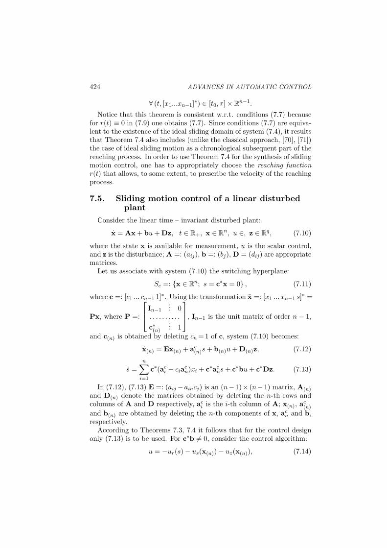
424 ADVANCES IN AUTOMATIC CONTROL
∀ (t, [x1...xn−1]∗) ∈ [t0, τ ]× Rn−1.
Notice that this theorem is consistent w.r.t. conditions (7.7) becausefor r(t) ≡ 0 in (7.9) one obtains (7.7). Since conditions (7.7) are equiva-lent to the existence of the ideal sliding domain of system (7.4), it resultsthat Theorem 7.4 also includes (unlike the classical approach, [70], [71])the case of ideal sliding motion as a chronological subsequent part of thereaching process. In order to use Theorem 7.4 for the synthesis of slidingmotion control, one has to appropriately choose the reaching functionr(t) that allows, to some extent, to prescribe the velocity of the reachingprocess.
7.5. Sliding motion control of a linear disturbedplant
Consider the linear time – invariant disturbed plant:
x = Ax + bu+ Dz, t ∈ R+, x ∈ Rn, u ∈, z ∈ Rq, (7.10)
where the state x is available for measurement, u is the scalar control,and z is the disturbance; A =: (aij), b =: (bj), D = (dij) are appropriatematrices.
Let us associate with system (7.10) the switching hyperplane:
Sc =: x ∈ Rn; s = c∗x = 0 , (7.11)
where c =: [c1 ... cn−1 1]∗. Using the transformation x =: [x1 ... xn−1 s]∗ =
Px, where P =:
In−1... 0
. . . . . . . . . .c∗(n)
... 1
, In−1 is the unit matrix of order n− 1,
and c(n) is obtained by deleting cn =1 of c, system (7.10) becomes:
x(n) = Ex(n) + ac(n)s+ b(n)u+ D(n)z, (7.12)
s =n∑
i=1
c∗(aci − ciac
n)xi + c∗acns+ c∗bu+ c∗Dz. (7.13)
In (7.12), (7.13) E =: (aij −aincj) is an (n−1)× (n−1) matrix, A(n)
and D(n) denote the matrices obtained by deleting the n-th rows andcolumns of A and D respectively, ac
i is the i-th column of A; x(n), ac(n)
and b(n) are obtained by deleting the n-th components of x, acn and b,
respectively.According to Theorems 7.3, 7.4 it follows that for the control design
only (7.13) is to be used. For c∗b 6= 0, consider the control algorithm:
u = −ur(s)− us(x(n))− uz(x(n)), (7.14)

A survey on flow-invariance based results in control systems 425
ur(s) = ρs+ δr, δr =
δ0, s < 0,
0, s = 0,
−δ0, s > 0,
, (7.15)
us(x(n)) =∑i∈J
ψixi, ψi =
βi, xis < 0,
αi, xis > 0,(7.16)
uz(x(n)) =
β0, s < 0,
α0, s > 0,(7.17)
where ur(s), us(x(n)) and uz(x(n)) have to control the reaching process,the ideal sliding motion, and the disturbance rejection respectively; ρ,δ0, αi, βi, (i ∈ J =: =: i ∈ 1, 2, ..., n − 1; c∗(ac
i − ciacn) 6= 0), and
α0, β0 are adjustable parameters. Using (7.7) for (7.13) the followingresult can be formulated.
Theorem 7.5 S is the ideal sliding domain for system (7.10), (7.14),with, c∗b 6= 0, if and only if
αic∗b ≥ c∗(aci − ciac
n), βic∗b ≤ c∗(aci − ciac
n), i ∈ J, (7.18)
α0c∗b ≥ supt
c∗Dz(t), β0c∗b ≤ inft
c∗Dz(t).
In order to design the reaching process as a precursor of the idealsliding motion, let us use the following reaching function:
r(t) =
[(|s0|+ δ)e−λ(t−t0) − δ
]sgn(s), t ∈ [t0, τ ],
0, t ∈ (τ, tf ),(7.20)
where s0 =: s(x0) = s(x(t0)), and δ > 0, λ > 0, τ > t0 are pre-assignableparameters. Using Theorem 7.4-3 (1 and 2 are satisfied with r(τ) = 0,τ = = t0 + λ−1 ln (1 + |s0|/δ) > t0), with (7.15) – (7.17), under (7.18),(7.19), one can formulate the following result.
Theorem 7.6 For each pair (t0,x0) ∈ R+× (Rn \S) the state of system(7.10), (7.14), with c∗b 6= 0, reaches ideal sliding domain S if and onlyif
ρc∗b ≥ c∗acn + λ, δ0c∗b ≤ c∗ac
n. (7.21)
The equations (7.14) – (7.17) and the inequalities (7.18), (7.19) and(7.21) define the (variable) structure and the adjustable parameters ofthe controller in order to fulfil requirements 1 and 2 from 7.1.

426 ADVANCES IN AUTOMATIC CONTROL
By solving the equation s = 0 (according to (7.13)) w.r.t. u and re-placing the result into (7.12) (s=0), one obtains the ideal sliding equa-tion:
x(n) = A1x(n) + D1z, (7.22)
where matrices A1 and D1 can be appropriately calculated. If rankb =rank [b, D], then D1 =0 and the disturbance rejection is ensured.
The stability of system (7.22) depends only on A1 and may be im-proved (requirement 3 from 7.1) by an additional state feedback. Thus,the state trajectories of system (7.10), (7.14) evolve with pre-assignablevelocity from each initial state x0 ∈ Rn\S towards ideal sliding domainS and then towards the final equilibrium state x=0.
8. ConclusionsThe flow-invariance method proves to be an efficient tool for a more
subtle characterization of the temporal evolution of the dynamical sys-tems. It certainly occasions a deeper insight into the system behav-ior, fact which becomes extremely relevant when the flow-invariant setconsidered in the state space is a time-dependent hyper-interval. Inthis case, a componentwise characterisation is available for the statevariables. Such a characterisation is useful especially when the statevariables present different importance for the normal system evolution,unlike the usual evaluation ensured by a norm-based characterisation(which is rather global and, consequently, it does not allow accurate dis-tinctions, when necessary, between the individual dynamics of the statevariables). Generally speaking, the corresponding results of the statecomponentwise characterisation have the form of necessary and sufficientconditions that analytically are expressed by differential or algebraic in-equalities. These results are interesting not only at the theoretical levelas yielding non-conventional approaches to system analysis and design,but also from the point of view of their applicability to large classes ofreal dynamical systems encountered in engineering (electric circuits andnetworks, neuronal networks, control systems), biology, ecology, pharma-cokinetics etc. In such cases, meaningful and significant non-standardknowledge may be gained that accurately enlighten refined aspects oftheoretical and practical interest for various applications.
In this context, the main conceptual sphere developed in the paperrefers to the componentwise asymptotic stability, whose construction re-lies, as preliminaries, on the analysis of constrained evolution of dynam-ical systems, and later on, is able to accommodate synthesis problemscovering observer and state feedback design, as well as sliding motioncontrol. Thus, the overall approach is founded on the notion of T U X –

A survey on flow-invariance based results in control systems 427
constrained evolution of a continuous-time dynamical system (Definition2.1) which can be characterized in terms of flow invariance (Theorem2.1), so as a noticeable particularization can be obtained when a spe-cial type of constraints, consisting in time-dependent hyper-intervals, isconsidered for the state and input variables (Theorem 2.2 - the generalcase, Theorem 2.3 - the linear, time-invariant case).
This background allows focusing on the free dynamics and definingthe CWASh and global CWASh properties (Definitions 3.1 and 3.2, re-spectively) for the existence of which necessary and sufficient conditionsare derived (Theorems 3.1, 3.2 – the general case, Theorems 3.3, 3.4 – thelinear, time-invariant case). A refinement of the CWASh requirementsleads to the CWEAS and global CWEAS concepts (Definitions 3.3 and3.4, respectively), which can be characterized algebraically (Theorems3.5, 3.6 – the general case, Theorems 3.7, 3.8 – the linear, time-invariantcase). By exploiting CWEAS, the componentwise absolute stability isintroduced for a class of nonlinear systems (Definition 3.5) and a neces-sary and sufficient condition for its existence is given (Theorem 3.9).For the case of linear, time-invariant systems, two results exploringthe eigenvalue location (Theorems 3.10, 3.11) are used to analyze theCWEAS robustness under unstructured and structured perturbations(Theorem 3.12 and Theorem 3.13, respectively). Remaining within theframework of linear dynamics, the study of the free response based onflow-invariance is extended for interval matrix systems (Theorems 4.1,4.2), offering a nice and natural generalization of the results on CWASh
and CWEAS previously reported, in the case of constant coefficients(Theorems 4.3, 4.5 and Theorem 4.6, respectively). This study also al-lows a refined interpretation of Hurwitz stability for interval matrices(Theorems 4.4).
The usage of flow-invariance method in exploring free dynamics is fur-ther applied for a class of nonlinear uncertain systems, yielding charac-terizations expressed in terms of nonlinear differential inequalities withconstant coefficients (Theorems 5.1, 5.2, 5.3); the nonlinearity of thedynamics involves a detailed discussion on the geometry of the flow-invariant time-dependent hyper-intervals (Theorems 5.4, 5.5, 5.6). Re-lying on some intermediary results (Theorems 5.7, 5.8, 5.9), it is shownthat the CWASh of the equilibrium state 0 of the nonlinear uncertainsystem is equivalent to the standard asymptotic stability of the equilib-rium state 0 of a differential equation with constant coefficients (Theo-rem 5.10); along the same lines, a sufficient condition is also given (The-orem 5.11), presenting the advantage of a simpler manipulation. Unlikethe linear dynamics previously investigated, the existence of CWEAS re-quires a special form for the state-space equations (Theorem 5.12), but

428 ADVANCES IN AUTOMATIC CONTROL
for such special forms, CWEAS is equivalent to CWASh (Theorem 5.15),as in the linear case. Moreover, a similarity with the linear case can alsobe found with regard to the algebraic characterization of CWEAS (The-orems 5.13, 5.14, 5.16, 5.17, 5.18). A necessary and sufficient conditionfor CWEAS of the nonlinear uncertain system is CWEAS of the intervalmatrix system which represents the linear approximation of the former(Theorem 5.19).
CWEAS principles can be exploited to incorporate typical problems oflinear system analysis/synthesis such as detectability and stabilizabilityredefined in the sense of componentwise constrained evolutions (Defini-tions 6.1,6.2, 6.3 and Definition 6.4, respectively), instead of the classicalformulations based on global approaches in terms of vector norms. ThusCWEAS detectability and CWEAS stabilizability are studied in con-junction with the design of CWEAS observers (Theorems 6.1, 6.2, 6.3,6.4, 6.5) and CWEAS state feedback control (Theorems 6.6, 6.7, 6.8,6.9), respectively.
The flow-invariance method gives an appropriate framework to dealwith sliding motion by using the notions of negatively and positivelyflow-invariant sets (Definition 7.1) and contextually defining the idealsliding motion domain (Definition 7.2). Relying on two preparatoryresults (Theorems 7.1, 7.2), the approach first focuses on ideal slidingmotions (Theorems 7.3, 7.4) and afterwards emphasis is placed on slidingmotion control of disturbed plants with linear dynamics (Theorems 7.5,7.6).
Far from scrutinizing the whole research potential offered by the ap-plicability of flow invariance in control system analysis and design, thissurvey paper creates an overview of most noticeable results emergedfrom the main concept of componentwise asymptotic stability. Fur-ther investigations can be directed towards various objectives pertain-ing to linear and nonlinear system theory, such as: CWEAS preserva-tion under linear transformations of the state-space variables, connec-tions between CWEAS stabilizability/detectability and standard strate-gies based on eigenvalue assignment, links between CWEAS stabilizabil-ity/detectability and linear quadratic problems, componentwise asymp-totic stability of different classes of nonlinear systems etc. Along thesame lines, a special remark deserves the new orientation of the flow-invariance instruments towards the discrete-time dynamics, which wasjust simply mentioned in the introductory section, without any detailsin the text, as being beyond the scope of the current survey.

A survey on flow-invariance based results in control systems 429
List of acronymsAS asymptotic stability (as a compound noun), or
asymptotically stable (as a compound adjective)CAS componentwise absolute stability (as a compound noun), or
componentwise absolutely stable (as a compound adjective)CCE componentwise constrained evolutionCWASh componentwise asymptotic stability w.r.t. h (as a compound
noun), orcomponentwise asymptotically stable w.r.t. h (as a compoundadjective)
CWEAS componentwise exponential asymptotic stability (as a compoundnoun), orcomponentwise exponential asymptotically stable (as a compoundadjective)
DE differential equationDI differential inequalityES equilibrium stateFI flow-invariance (as a compound noun), or
flow-invariant (as a compound adjective)IMS interval matrix systemLECM linear elementwise C-majorantNUS nonlinear uncertain systemPS positive solutionTDRS time-dependent rectangular setw.r.t. with respect to
References[1] Naugmo, M., Uber die Lage der Integralkurven gewohnlicher Differentialgle-
ichungen, Proc. Phys. Math. Soc. Japan, 24, pp. 551-559, 1942.
[2] Hukuhara, M., Sur la theorie des equations differentieles ordinaries, J. Fac. Sci.Univ. Tokio, Math. 7, no. 8, pp. 483-510, 1954.
BREZIS, H., On a characterization of flow-invariant sets, Comm. Pure Appl.Math., 23, pp. 261-263, 1970.
[3] Crandall, M. G., A generalization of Peano’s existence theorem and flow-invariance, Proc. Amer. Math. Soc., 36, pp. 151-155, 1972.
[4] Martin, R. H. jr., Differential equations on closed subsets of a Banach space,Trans. Amer. Math. Soc., 179, pp 399-414, 1973.
[5] Pavel, H. N., Differential Equations, Flow-invariance and Applications, Pitman,Boston, 1984.
5MOTREANU, D., PAVEL, H. N., Tangency, flow-invariance for differential
equations and optimisation problems, Marcel Dekker, New York, 1999.
[6] Voicu, M., State constraints and asymptotic stability of linear constant dynamicalsystems, Bul. Inst. Politehnic Iasi, XXVII (XXXI), s. III, pp. 57-60, 1981.
[7] Voicu, M., Componentwise asymptotic stability of the linear constant dynamicalsystems, (Al 2-lea Simp. Nat. de Teoria Sist., Univ. din Craiova, vol. I, pp. 69-75, 1982); Preprint Series in Math. of “A. Myller” math. Seminar, University ofIasi, 5, pp. 1-14, 1982.

430 ADVANCES IN AUTOMATIC CONTROL
[8] Voicu, M., Free response characterization via flow-invariance, 9-th WorldCongress of Int. Fed. of Automatic Control, Budapest; Preprints, 5, pp. 12-17,1984.
[9] Voicu, M., Componentwise asymptotic stability of linear constant dynamical sys-tems, IEEE Trans. on Aut. Control, AC-29, no. 10, pp. 937-939, 1984.
[10] Voicu, M., Evolution on control and state hyper-intervals, 6-th Internat. Conf.Control Syst. & Comp. Sci., Bucharest; Preprints, 1, pp. 81-83, 1985.
[11] Voicu, M., Structural properties of the spatial manipulating systems in connec-tion with the state and control constraints, IFAC Symposium on Robot Control1985, Barcelona; pp. 425-428.
[12] Voicu, M., Tehnici de analiza a stabilitatii sistemelor automate (Stability Anal-ysis Techniques of the Automatic Control Systems), Editura Tehnica, Bucuresti,1986.
[13] Voicu, M., On the application of the flow-invariance method in control theory anddesign, 10-th World Congress of Int. Fed. of Aut. Control, Munich; Preprints,8, pp. 364-369, 1987.
[14] Voicu, M., On the existence of limit cycles (in Romanian), Al 2-lea Simp.“Structuri, algoritmi si echipamente de conducere a proc. ind.“, Inst. Polit. Iasi;Preprints, pp. 39-43, 1989.
[15] Voicu, M., Sufficient existence conditions of limit cycles, Bul. Inst. PolitehnicIasi, XXXII (XXXVI), s. III, pp. 23-26, 1990.
[16] Voicu, M., Flow-invariance method and componentwise absolute stability;applications in biotechnological systems, Conferenece presented at Lab.d’Automatique de Grenoble, 1993.
VOICU, M., Sufficient conditions for Hurwitz and Schur polynomials, Bul. Inst.Politehnic Iasi, XLIV (XLVII), s. IV, pp. 1-6, 1998.
[17] Voicu, M., Componentwise absolute stability of endemic epidemic systems, Work-shop on “Theories of Popov-type”, Romanian Academy, Bucharest; Preprints,pp. 97-104, 1999.
[18] Pastravanu, O., Voicu, M., Flow-invariant rectangular sets and componentwiseasymptotic stability of interval matrix systems, 5-th European Control Conf.,Karlsruhe; CDROM, rubicon-Agentur fur digitale Medien, Aachen, 16 p, 1999.
[19] Pastravanu, O., Voicu, M., Robustness analysis of componentwise asymptoticstability, 16-th IMACS World Congress, Lausanne; CDROM, imacs (ISBN 395222075 1 9), 2000.
[20] Pastravanu, O., Voicu, M., Preserving componentwise asymptotic stability underdisturbances, Rev. Roum. Sci. Techn., ser. Electrot. Energet., 45, no. 3, pp. 413-425, 2000.
[21] Pastravanu, O., Voicu, M., Robustness of componentwise asymptotic stability fora class of nonlinear systems, Proc. of Romanian Academy, ser. A, 1, 1-2, 2001,61-67.
[22] Pastravanu, O., Voicu, M., Componentwise characterization of the free responsefor a class of nonlinear systems, 13th International Conf. on Control Systemsand Computer Science, University Politehnica of Bucharest; Proceedings, pp.50-55, 2001.

A survey on flow-invariance based results in control systems 431
[23] Pastravanu, O., Voicu, M., Dynamics of a class of nonlinear systems under flow-invariance constraints, 9-th IEEE Med. Conf. on Control and Aut. (MED’01),Dubrovnik; CD-ROM (ISBN 953 6037 35 1), Book of abstracts (ISBN 953 603734 3); c©KoREMA (Zagreb), 6p, 2001.
[24] Pastravanu, O., Voicu, M., Componentwise asymptotic stability of a class of non-linear systems. 1st IFAC Symposium on System Structure and Control (SSSC01), August 29-31, 2001, Czech Techn. Univ. of Prague; Book of Abstracts, p.28; CD-ROM, 078, 6 p, 2001.
[25] Pastravanu, O., Voicu, M., Flow-invariance in exploring stability for a classof nonlinear uncertain systems, 6th European Control Conf., Porto, Sept. 4-7,2001; CD-ROM, 6 p, 2001.
[26] Pastravanu, O., Voicu, M., Interval matrix systems – flow-invariance andcomponentwise asymptotic stability, J. Diff. & Int. Eq, Nov., 2002 (acceptedfor publication).
[27] Hmamed, A., Componentwise stability of continuous-time delay linear systems,Automatica, 32, no. 4, pp. 651-653, 1996.
[28] Hmamed, A., Componentwise stability of 1D and 2D linear discrete-time sys-tems, Automatica, 33, no. 9, pp. 1759-1762, 1997.
[29] Hmamed A., Benzaouia A., Componentwise stability of linear systems: a non-symmetrical case, Int. Journal Robust Nonlin. 7, no. 11, pp. 1023-1028, 1997.
[30] Chu, T. G., Convergence in discrete-time neural networks with specific perfor-mance, Phys. Revue E, 6305, pp. 1904- + Part 1, art. No. 051904, May 2001.
[31] Voicu, M., State feedback matrices for linear constant dynamical systems withstate constraints, 4-th Internat. Conf. Control Syst. & Comp. Sci., UniversityPolitehnica of Bucharest; Preprints, 1, pp. 110-115, 1981.
[32] Voicu, M., Componentwise stabilization of constant linear dynamical systems (inRomanian), 3-th MSIOPT Symp., University of Galati, Preprints, pp. 103-108,1982.
[33] Voicu, M., On the determination of linear state feedback matrix, 5-th Inter-nat. Conf. Control Syst. & Comp. Sci., University Politehnica of Bucharest;Preprints, 1, pp. 119-123, 1983.
[34] Voicu, M., Gerschgorinsche Kreise und die komponentenweise Stabilisierung,Bul. Inst. Politehnic Iasi, XXXI (XXXV), s. III, pp. 45-50, 1985.
[35] Voicu, M., Ein Anwendungsbeispiel der Komponentenweisen Stabilisierung, Bul.Inst. Politehnic Iasi, XXXI (XXXV), s. III, pp. 57-60, 1985.
[36] Voicu, M., A sufficient asymptotic stability condition for discrete systems, Bul.Inst. Politehnic Iasi, XXXII (XXXVI), s. III, pp. 38-39, 1986.
[37] Voicu, M., System matrix with prescribed off-diagonal entries obtained via statefeedback, Bul. Inst. Politehnic Iasi, XLIII (XLVII), s. IV, pp. 5-9, 1997.
[38] Voicu, M., Bulea, M., Pole assignment in a region of complex plane via linearprogramming (in Romanian), Conf. Nationala de Electronica, Telecomunicatii,Automatica si Calculatoare, Bucuresti; Preprints, TS, pp.153-165, 1982.
[39] Voicu, M., Observing the state with componentwise decaying error, Systems &Control Letters, 9, pp. 33-42, 1987.

432 ADVANCES IN AUTOMATIC CONTROL
[40] Pastravanu O., Voicu, M., State feedback design for componentwise exponentialasymptotic stability, Int. Symp. on Aut. Control and Comp. Sci. (SACCS 2001),Techn. Univ. of Iasi; CD-ROM, 6 p, 2001.
[41] Voicu, M., Morosan, B. I., A theorem on structure-variable systems (in Roma-nian), Al 2-lea Simpozion “Structuri, algoritmi si echipamente de conducere aproceselor industriale“, Inst. Politehnic Iasi; Preprints, pp. 21-26, 1989.
[42] Voicu, M., Morosan, B. I., Existence problem of an ideal sliding domain (inRomanian), Zilele academice iesene, Academia Romana, Fliala Iasi, 7 p., 1989.
[43] Voicu, M., Morosan, B. I., State space flow structure induced by sliding motioncontrol, Bul. Inst. Politehnic Iasi, XXXV (XXXIV), s. III, pp. 25-29, 1989.
[44] Voicu, M., Morosan, B. I., Flow structure involving reaching of the sliding sur-face in variable structure systems, Int. Conf. on El. Drives, Univ. of Brasov;Preprints, G4, 1991.
[45] Voicu, M., Morosan, B. I., Variable-structure controller for feedback positioningof d.c. electric motor, Rev. Roum. Sci. Techn., ser. Electrot. Energet., 36, no.2, pp. 12-24, 1991.
[46] Voicu, M., Morosan, B. I.,Flow invariance based characterization of quasi-slidingmotion, International Workshop on Applied Automatic Control, Czech TechnicalUniversity of Prague; Preprints, pp.86-89, 1993.
[47] Voicu, M., Morosan, B. I., Variable-structure control characterization and designvia flow-invariance method, Int. J. Automation Austria, 5, no. 1, pp.12-24, 1997.
[48] Morosan, B. I., On the sliding conditions in sampled-data systems, Bul. Inst.Politehnic Iasi, XXXVII (XLI), s. VI, pp. 18-22, 1991.
[49] Morosan, B. I., Quasi-sliding mode with integral control for a second order un-certain plant, Int. Symp. Aut. Control & Comp. Sci., Techn. Univ. of Iasi;Preprints, pp. 1-6, 1993.
[50] Morosan, B. I., Variable structure systems analysis with “MATHEMATICA”,Workshop on Computer Sci. Topics for Control Engrg. Educ., Vienna Universityof Technology; Proceedings SEFI, no. 10 (ISBN 2 87352 012 4), Bruxelles, 1993.
[51] Morosan, B. I., Discrete quasi-sliding mode control for coupled tanks system,Workshop on Automation and Control Technology Educ. 2001, Vienna Univer-sity of Technology; Proceedings SEFI, no. 2 (ISBN 2 87352 005 1), Bruxelles,1993.
[52] Morosan, B. I., Fuzzy control in quasi-sliding mode systems, Int. Workshop onFuzzy Technology in Automation and Intelligent Systems – “Fuzzy Duisburg’94”, University of Duisburg; Proceedings, pp. 155-161, 1994.
[53] Morosan, B. I., Digital variable-structure systems studied by flow-invariancemethod, Doctoral thesis (in Romanian), Technical University of Iasi, 1994.
[54] Morosan, B. I., VOICU, M., Flow-invariance method in general sliding modesystem, Technical Report, Delft University of Technology, 1993.
[55] Morosan, B. I., VOICU, M., General sliding mode systems analysis and designvia flow-invariance method, Studies in Informatics and Control, 3, no. 4, pp.347-365, 1994.
[56] VOICU, M., PASTRAVANU, O., Flow-invariance method in systems theory(in Romanian), Seminarul “Stabilitatea si robustetea sistemelor automate“,Academia Romana, Filiala Iasi, 12 p., 21-22.01.2000.

A survey on flow-invariance based results in control systems 433
[57] Ursescu, C., Caratheodory solutions of ordinary differential equations on locallycompact sets in Frechet spaces, Preprint Series in Math., University of Iasi, 18,pp. 1-27, 1982.
[58] Voicu, M., PASTRAVANU, O., Componentwise asymptotic stability induccedby symmetrical polyhedral time-dependent constrants, IFIP Conf. “Analysis andOptim. Diff. Syst.”, Sept. 2002, Constanta (accepted for presentation).
[59] Pastravanu, O., VOICU, M., Infinity norm in analysis of componentwiseasymptotic stability, IFIP Conf. “Analysis and Optim Diff. Syst.”, Sept. 2002,Constanta (accepted for presentation).
[60] Siljak, D. D., When is a complex ecosystem stable? Math. Biosci., 25, pp. 25-50,1975.
[61] Siljak, D. D., Connective stability of competitive equilibrium, Automatica, 11,pp. 389-400, 1975.
[62] Sezer M. E., Siljak D. D., On stability of interval matrices, IEEE Trans. on Aut.Control, AC-39, pp. 368-371, 1994.
[63] Chen J., Sufficient condition on stability of interval matrices: connections andnew results, IEEE Trans. on Aut. Control, AC-37, pp. 541-544, 1992.
[64] Pastravanu, O., VOICU, M., Dynamics of a class of uncertain nonlinear systemsunder flow-invariance constraints, Int. J. Math. and Math. Scie. (accepted forpublication).
[65] Tschernikow, S. N., Lineare Ungleichungen, Deutscher Verlag der Wiss., Berlin,1971.
[66] Barbu, V., Precupanu, Th., Convexity and optimisation in Banach spaces, Edi-tura Academiei, Bucuresti, Reidel, Dordrecht, 1986.
[67] Utkin, V. I., Sliding modes and their application in variable structure systems,MIR, Moscow, 1978 (English transl. of Russian edition, Nauka, Moscow, 1974).
[68] Utkin, V. I., Sliding mode in control optimisation, Springer-Verlag, Berlin, 1992.


ADDENDUM
BRIEF HISTORY OF THE AUTOMATIC CONTROL DEGREE COURSE AT TECHNICAL UNIVERSITY “GH. ASACHI” OF IAŞI
Corneliu Lazar, Teohari Ganciu, Eugen Balaban, Ioan Bejan Technical University “Gh. Asachi” of Iaşi Dept. of Automatic Control and Industrial Informatics e-mail: clazar, tganciu, [email protected]
Abstract: The Faculty of Automatic Control and Computer Engineering, one of the leading training and research centre in the field of automatic control and computer engineering from Romania, during the university year 2002 – 2003 has celebrated 40 years from the appearance of the first courses in the above mentioned field and 25 years from the emergence of the Automatic Control and Computer Engineering degree course. On this occasion, some of the most significant scientific achievements have been put together in this article, as a brief history of the Automatic Control degree course at Technical University “Gh.Asachi” of Iaşi.
1. Origin (the end of 50s– 1977) Control engineering saw rapid development in many countries in the
period immediately following the Second World War. Engineers and scientists concerned with control problems have formed new professional groupings and university courses dedicated to this subject have arisen. At the same time, research groups have been set up both in the industrial and in the academic communities.
In the above context, control engineering has started at the Technical University “Gh. Asachi” of Iaşi in the 50s. The Department of Electrical Drives from the Electrical Engineering Faculty was approaching issues in control engineering, which were introduced as chapters in the courses “Electrical Drives” and “Electromechanical Equipment”. The first course actually entitled “Automation” was an optional course and it was initiated in

ADVANCES IN AUTOMATIC CONTROL 436
the same period by professor Nicolae Boţan. As a result of their didactic and research activities, Nicolae Botan, Ioan Bejan and Eugen Balaban published the first book, named “Eletromechanical Drives and Automation”, in the field of automatic control at “Editura didactică şi pedagogică”, Bucureşti in 1962.
Other compulsory courses have been established prior to 1962, which were mainly focused on the requirements of electromechanical engineering and electrical power engineering programs. This was the case with the course of “Automation and Remote Control” (within the two degree courses) and the course on “Relay protection” (for the electrical power engineering program) taught by professors Leopold Sebastian and Ioan Bejan. In 1967, Ioan Bejan and Gherghina Balaban published the first course in control, entitled “Automation and Remote Control” at the publishing house of the University of Medicine and Pharmacy “Gr. T. Popa” of Iaşi.
In the 60s and the beginning of the 70s, the course of “Automation and Remote Control” has known a rapid development, e.g. the course “Automatic Control” (Leopold Sebastian) started at the electromechanical engineering program and the course “Automation of Electrical Power Systems” (Ioan Bejan) was introduced for the electrical power engineering program. New optional courses have also simultaneously appeared for electrical engineering, such as: “Logical Circuits and Sequential Control Systems” (Corneliu Hutanu), “Servomechanisms” (Iosif Olah), “Computer Controlled Processes” (Simona Caba) and “Advanced Automation” (Gherghina Balaban and Iosif Olah).
Under the supervision of professors Ioan Bejan and Leopold Sebastian extensive research have been carried out at the Department of Electrical Drives ranging from control theory problems (nonlinear systems, identification, adaptive and optimal control, controller tuning) to the application of control methods to areas of thermal processes, electrical drives, electrical power systems, relay protection systems, servomechanisms or machines tools control. The above mentioned professors have initiated PhD positions in Industrial Automation (Leopold Sebastian – 1966) and in Electrical Power System Automation (Ioan Bejan – 1972). Then, two research groups have emerged, headed by Leopold Sebastian for the electrical engineering program (Eugen Balaban, Corneliu Hutanu, Iosif Olah, Corneliu Botan, Teohari Ganciu and Simona Caba) and Ioan Bejan for the electromechanical power engineering programme, respectively (Gherghina Balaban, Ioan Titaru, Mihail Voicu, Cristea Pal and Dumitru Asandei).
Due to the fact that these groups were at that time the only ones offering courses in automatic control, one of the main tasks was from the very beginning to write manuals and monographs. In the 70s, several well-known books have been published in Romanian, e.g.:
• L. Sebastian, “Automatic Control”, Editura didactică şi pedagogică, Bucureşti, 1975;

ADDENDUM Brief history of automatic control degree course 437
• I. Bejan, “Automation and remote control of electrical power systems”, Editura didactică şi pedagogică, Bucureşti, 1976;
• I. Bejan, “Magnetic amplifier for control systems”, Editura Tehnică, Bucureşti, 1972;
• N. V. Boţan, “Speed control of electrical drives”, Editura Tehnică, Bucureşti, 1974;
• N. V. Boţan, “Electrical drives control”, Editura Tehnică, Bucureşti, 1977.
In the above mentioned period, PhD degrees in the field of automatic control have been obtained by Mihail Voicu, Corneliu Botan, Gherghina Balaban and Iosif Olah.
Also in the same period, the members of the automatic control group were awarded the following prizes:
• the Ministry of Education prize - Ioan Bejan, Nicolae Botan, Leopold Sebastian, Eugen Balaban, Gherghina Balaban and Mihail Voicu;
• professor emeritus awarded by the Ministry of Education – Ioan Bejan, Eugen Balaban and Iosif Olah.
2. First automatic control program (1977 – 1990) In 1977, a five years course entitled “Automatic Control and Computer
Engineering” has been developed within the Faculty of Electrical Engineering. This came as a response to the demands from industry, which began to require well prepared engineers in the fields of control and computer engineering.
A study program of two years began in 1977. There were two groups of first-year students which took entrance examination at the new degree course and other two of second-year students transferred from the electrical and electronic engineering programs. Each group of students had separate curricula, one for Automatic Control within the Electrical Drives Department and the other for Computer Engineering functioning at the Electronic Department.
As it has been mentioned in the previous section, at the Electrical Drives Department there were already teaching staff and research laboratories in the field of control engineering. The control team elaborated the first Automatic Control curriculum that comprised courses of System theory, Digital control systems, Analogue control systems, System identification, Hydraulic and pneumatic control equipment, Control system design, Systems and equipment for process control and Optimal control. The scientific research of the automatic control staff has known a significant progress characterized by several research projects, the publishing of monographs and participation at international conferences.

ADVANCES IN AUTOMATIC CONTROL 438
In the 80s, the following new areas of research have appeared: flow-invariance in control theory, computer controlled processes, machine vision, pattern recognition, computer aided control engineering and robotics. In 1983 professor Corneliu Hutanu’s book “Digital circuits and sequential control systems” was published at “Junimea” publishing house from Iaşi and professor Mihail Voicu published an important monograph at “Editura Tehnică, Bucureşti” in 1986 entitled “Stability analysis techniques for control systems”.
The deep crisis experienced by Romania as a country in the 80s particularly affected higher education and inevitably, also the automatic control teaching staff, which faced serious problems. For example only three teaching assistants were admitted as PhD students in that period in the field of automatic control. It was extremely difficult, from an administrative point of view, to publish abroad or to participate at international conferences. However, under these severe conditions, 10 papers have still been published in important foreign journals by Mihail Voicu, Leopold Sebastian, Octavian Pastravanu and Teohari Ganciu and 9 papers appeared in the proceedings of international conferences. In this respect, the participations of professor Mihail Voicu at the 9th IFAC World Congress in Budapest (1984) and at the 10th IFAC World Congress in Munich (1987) can be considered as remarkable achievements. Also, Octavian Pastravanu has presented papers at the international conferences ”Symposium on Systems Science IX” organized by University of Wroclaw (1986), “European Congress of Simulation” organized by Czechoslovak Academy of Science in cooperation with IMACS at Prague (1987) and the 4th International Symposium on Systems Analysis and Simulation organized by DDR Academy of Science in cooperation with IMACS at Berlin (1988), and Corneliu Lazar has presented a paper at “The 3rd International Conference on Automatic Image Processing” organized by Scientific Technological Society for Measurement and Automatic Control and DDR Academy of Science at Leipzig (1989).
The main difficulties in teaching and research activities were caused by the lack of computer facilities. Notable efforts have been done by the teaching assistants Octavian Pastravanu and Corneliu Lazar in the mid 80s, which were supported by the dean of the faculty, professor Ioan Bejan and by professor Mihail Voicu, in order to achieve proper computer equipment and software and to develop laboratories for computer aided control engineering.
Beginning with 1987, the control group formed within the teaching staff of the Electrical drives Department organized every two years the national scientific symposium “Structures, Algorithms and Equipment for Process Control”.
In the mid 80s, professor Teohari Ganciu concentrated his efforts on the foundation of an important research centre – the Iaşi branch of the “Automation Design Institute”.
ADDENDUM Brief history of automatic control degree course 439
3. The Faculty of Automatic Control and Computer Engineering
As a direct consequence of the profound changes experienced by the Romanian nation in 1989, the Romanian higher educational system has known a lively development. The Faculty of Electrical Engineering has split in 1990 in three faculties. One of these, the Faculty of Automatic Control and Computer Engineering has been founded at the initiative and due to the efforts of the teaching staff from the degree course “Automatic Control and Computer Engineering” of the former Electrical Engineering Faculty. Professor Corneliu Hutanu was the first dean of the faculty from 1990 to 1992. From the beginning, the faculty had two departments, Automatic Control and Industrial Informatics and Computer Engineering, each of them offering the following degree courses: Automatic Control and Industrial Informatics and Computer Engineering, respectively.
The first head of the Automatic Control and Industrial Informatics department, professor Mihail Voicu, together with the department staff began in 1990 to develop a new curriculum in Automatic Control and Industrial Informatics. It must be noted that this curriculum was also influenced by a consultative council of the Automatic Control professors from Romania in order to maintain certain compatibilities between similar curricula introduced in other university centers of the country. Starting with the beginning of the 90s, this curriculum has been changed and improved on a yearly basis, also based on the knowledge and the experience of other European universities, with which several contacts have been established in the framework of EU programs.
Due to the efforts of Mihail Voicu and Octavian Pastravanu, TEMPUS Joint European Projects (JEP) have been developed in collaboration with the Control Engineering Departments of other European universities, e.g. JEP 0886/1990 "Higher Education in Control Engineering", JEP 02011/1991 "Improvement in Automatic Control Technologies", JEP 07101/1994 "Development in Romania of Short-Term Higher Education in Computing, Centered on Distributed Processing and Its Application", MJEP 11467/1996 “EU Compatible Training in Industrial Automation” – COMPANION. The last TEMPUS project of the 90’s, UM-JEP 13133/98 “Quality Management”, has been managed by Alexandru Onea and it has resulted in a significant contribution to the implementation of the quality assurance system of our faculty.
These projects also offered a good opportunity for establishing relationships between our department and other European universities, which materialized in the participation of all the teaching staff to workshops organized by the JEP members and dedicated to Control Engineering Education and in the acquisition of modern laboratory setup. Due to the JEP framework, most of the teaching staff and especially young PhD students had the possibility to attend training stages at the partner universities.

ADVANCES IN AUTOMATIC CONTROL 440
Based on TEMPUS programs, the “traditional” approach towards teaching has been modified substantially. The faculty has accepted and implemented the European Credit Transfer System (ECTS) starting with the academic year 1998 – 1999 and has made our teaching procedures compatible with similarly oriented universities in the world. This makes possible the exchange of students and academic staff and mutual recognition of qualifications.
The European Credit Transfer System formed the basis of future collaborations that continued after the end of the TEMPUS program. Thus, with some of the partner universities, the program Socrates-Erasmus began to grow at the end of the 90s. In the framework of this program, each year students from our department worked on the diploma project at the following universities: University of Gent - Department of Electrical energy, Systems & Automation, University of Sheffield - Department of Automatic Control and System Engineering, University of Duisburg - Department of Measurement and Control Engineering, Technical University of Vienna, Université Joseph Fourier – Laboratoire d’Automatique de Grenoble. Within this program, an important number of MSc and PhD students had also training stages. Since 1999 till now, in the framework of the Socrates – Erasmus program, professor Robin De Keyser from the University of Gent has taught each year a module of the Predictive Control Systems course for the MSc program of our department. At the same time, professors Corneliu Lazar and Octavian Pastravanu have taught mini-courses on Predictive Control and Process Modelling Using Bond Graph, respectively, in the last two years at the University of Ghent.
Together with the development of a new curriculum for the Automatic control program, at the beginning of the 90s, new teaching staff has been recruited from the research institutes and young graduates. In 1992 professor Mihail Voicu, who had a strong experience in managing research and teaching staff, has become the dean of the faculty. Since the same year, professor Ganciu has been the head of the department of Automatic Control and Industrial Informatics.
Also, it must be mentioned that due to the changes that took place in Romania at the beginning of 90s, besides professors Bejan and Sebastian, the professors Voicu, Hutanu, Balaban, Botan and Olah also have received the right to be PhD supervisors in Automatic Control. Thus, new research areas have appeared and a greater number of graduates in Automatic Control have become PhD students, which ultimately led to an increased research activity. As a result of this, the number of scientific works published in journals and at international conferences and congresses has also increased considerably.
At the end of the 90s, what seemed to be a “natural” development took place, and the research groups from the department of Automatic Control and Industrial Informatics merged and they formed the Automatic Control

ADDENDUM Brief history of automatic control degree course 441
and Applied Informatics (ACAI) Research Centre accredited by Ministry of Education and Research classified in the C category. ACAI is an interdisciplinary research centre managed by professor Mihail Voicu within the faculty of Automatic Control and Computer Engineering and its mission is to fulfill statements of the university and of the faculty within the field of Systems and Control Engineering by creating and sustaining a world class research group. The main directions of the scientific research are: System Theory, Robotics and CIM Optimal and Predictive Control, Artificial Intelligence in Process Control, Systems Identification and Fault Detection, Microprocessor Based Control Systems, CAD for Dynamic Systems. The activity of ACAI has been carried out in grants with the Ministry of Education and Research and industrial companies (grant directors: Mihail Voicu, Corneliu Botan, Corneliu Lazar). The ACAI research staff had a very productive period from 2000 to 2003, publishing 15 monographs and courses, 14 journal papers among which 16 in ISI journals and 121 conference papers.
Since 1998, the department of Automatic Control and Industrial Informatics offered a short cycle degree program of 3 years on Automation Equipment. The undergraduate program of 3 years curriculum represents in a way a compromise between the necessity for a graduate with a diploma from the Engineering College to be operational in his job and the possibility for him to go on with more advanced studies.
After graduating the long cycle degree program, the students who wish to continue their studies can choose to apply for master program – one year of specialization – which is organized in the area of Automatic Control, having the subjects: distributed parameter control systems, parallel programming algorithms and techniques, predictive control, parameter estimation, distributed control and artificial intelligence in control.
In September 1998, the faculty has been moved in a new building having 7700 m2 useful area with 2 amphitheatres, 7 lecture rooms, 30 laboratories and 32 offices for the teaching staff. The two departments of the faculty develop their activity in the new building beside the library and the Communication Centre of Technical University “Gh. Asachi” of Iaşi. It is important to say that the building has been started off at the beginning of the 90s at the initiative of professor Mihail Voicu, supported by professor Ioan Bejan to take the initial necessary steps at the Ministry of Education.
Unfortunately, the 90’s economic decline of Romania created serious problems regarding higher education financing. As a result of this, several young people from the teaching staff left the department trying to fulfill their professional careers in more developed countries. At the same time serious difficulties have appeared in providing facilities for teaching and research work. However, the department members could adapt to the new forms of financing by having access to external funds, mainly from the following

ADVANCES IN AUTOMATIC CONTROL 442
sources: European Trading Foundation – TEMPUS JEPs, Higher Education Financing Council of Ministry of Education, World Bank, Romanian Government and industrial companies.
Thus, during 1998 – 2003 the following five major projects have been financed by the World Bank and Romanian Government: System of Integrated Laboratories for Studying CIM (director Mihail Voicu – 193000 USD), Training Laboratory in the Field of Computer Aided Process Control (director Octavian Pastravanu – 150000 USD), Laboratory for Electrical Drives Control (director Corneliu Botan – 150000 USD), Integrated Laboratory for Studying, Designing and Implementation of Digital Structure for Process Control (director Teohari Ganciu – 150000 USD), Upgrading of the Short Cycle Degree Program on Automation Equipment (director Alexandru Onea – 35000 USD). There were also 2 individual projects only for the equipment acquisition: Microprocessor Based Control Systems (director Corneliu Hutanu – 5000 USD) and Digital Controller for Process Control (director – Corneliu Lazar – 5000 USD). These funds allowed the development of new laboratories and the update of most of the existent laboratories at our department with the following major facilities for teaching and research work:
• Flexible Manufacturing System containing two ABB robots (IRB 1400 and IRB 2400), machine tool (EMCO PC Mill), conveyor (FlexLink), computer vision system (OptiMaster), CAD system (8 PC stations); Robot Soccer System containing 8 MiaBot mobile robots and a computer vision system; Androtec mobile robot;
• Process control setups: FieldPoint Distributed Control System (National Instruments) for the distributed control of industrial processes, PROCON process control trainers for level, flow and temperature (Feedback), LEYBOLD and ELWE electrical drive control trainers, Twin Rotor MIMO System (Feedback), Moeller PLCs, Laboratory kits for teaching microprocessor based systems;
• Laboratory installation for making printed circuit boards (Lpkf Germany);
• Computers: 45 computers (IBM compatible) with operating systems and basic software, 5 analogue COMDYNA computers, 7 data acquisition cards – National Instruments ATMIO16E10 with starter Kit and related drivers;
• Software: CATIA V5R8 (CAD); Robot Studio (robot simulation software), Eclipse, RT++, AgentOCX, LPA Prolog, Flex, Agent Toolkit (artificial intelligence software), Sucosoft V5 (PLC software), Discovery computer control aided learning software, MATLAB- Simulink 6.0, HMI/SCADA software Lookout, Cadence software (OrCAD) for PCB design.
The above funds have also been used to purchase important textbooks in

ADDENDUM Brief history of automatic control degree course 443
the field of automatic control for the faculty library. They also contributed in the publishing of monographs and university manuals, the development of new courses in Automatic Control degree program, the finalization of PhD thesis and the participation at international conferences.
Based on the experience accumulated from the last TEMPUS project, Alexandru Onea initiated and led other two projects having the same theme, quality assurance in higher education: MATRA project – “Developing the national strategy in the field of quality assurance in higher education in Romania, financed by EU through the Dutch Government and the Leonardo da Vinci project – “Training in quality management system for information technology in higher education”.
In the period from 1990 until the present time the teaching staff of the department published 22 monographs, 31 manuals and courses and it largely participated in many international conferences both in the country and abroad. As a remarkable achievement, it can be mentioned the contribution to each edition of the European Control Conference from the beginning until now of professors Mihail Voicu and Octavian Pastravanu as well as the participation of the lecturers Letitia Mirea and Lavinia Ferariu at the 15th IFAC World Congress in Barcelona 2002.
After the foundation of the EU Control Association (EUCA), part of the research developed within our department became known for the scientific community of Automatic Control by a number of papers published in different editions of the European Control Conference (ECC). These papers focus on the following topics (i) AI techniques in identification and diagnosis (Marcu and Voicu - ECC'93, ECC'95; Marcu and Ferariu - ECC'99; Marcu and Matcovschi - ECC'99; Marcu and Mirea - ECC'01; Ferariu - ECC'03); (ii) Dynamics of systems with unknown parameters (Voicu and Pastravanu - ECC'95; Pastravanu and Voicu - ECC'97); (iii) Time-dependent invariant sets and componentwise stability (Pastravanu and Voicu - ECC'99, ECC'01, ECC'03; Matcovschi and Pastravanu - ECC'03).
Due to his outstanding contributions professor Mihail Voicu was elected correspondent member of the Romanian Academy of Technical Sciences in 1997 and from 1998 he becomes senior member of IEEE. Also, he has received the “Aurel Vlaicu” prize of the Romanian Academy for the year 1987 (awarded 1990) for the papers:
• M. Voicu, Observing the State with Componentwise Exponentially Decaying Error. Systems & Control Letters 9 (1987), pp. 33 – 42.
• M. Voicu, On the Application of the Flow-Invariance Method in Control Theory and Design. 10th World Congress of International Federation of Automatic Control, Munich, July 26–31, 1987. Preprints, vol. VIII, pp. 364–369.
Starting with 2001 the department offered a new degree course on Industrial Informatics and from 2002 the degree course on Automatic

ADVANCES IN AUTOMATIC CONTROL 444
Control and Industrial Informatics became Automatic Control and the short cycle degree course Automation Equipment was renamed Automation.
The numerous contacts with the western universities permitted the change of the national scientific symposium of the faculty in the international symposium on Automatic Control and Computer Science organized every two years, namely in 1993 and 1995 and every three years afterwards.
Since 1991, owing to the initiative of professor Mihail Voicu, the Bulletin of the Polytechnic Institute of Iaşi has a new fascicule (1-4) with Section 4 dedicated to Automatic Control and Computer Engineering, editors being from the beginning till now Octavian Pastravanu, Doru Panescu and Alexandru Onea. This journal allowed the specialists in the automatic control field to point out the results of their scientific research activity.
At the present time, the Automatic Control degree program at the Technical University “Gh. Asachi” of Iaşi is carried out by the following teaching staff, of the Automatic Control and Industrial Informatics Department from the Faculty of Automatic Control and Computer Engineering:
• Professors: Eugen Balaban, Ioan Bejan (honorary professor), Corneliu Botan, Teohari Ganciu (head of the Department), Corneliu Hutanu, Corneliu Lazar (scientific chancellor of the Faculty Council), Iosif Olah, Cristea Pal (head of the Iaşi branch of the Romanian Society of Automatic Control and Technical Informatics), Doru Panescu (deputy head of the Department), Octavian Pastravanu, Leopold Sebastian (honorary professor) Mihail Voicu (dean of the Faculty)
• Associate Professors: Stefan Dumbrava, Lucian Mastacan, Mihaela Matcovschi, Alexandru Onea (editor of the Automatic Control Section of the Bulletin of the Polytechnic Institute of Iaşi), Andrei Pricop, Gabriela Varvara
• Lecturers: Catalin Calistru, Lavinia Ferariu, Letitia Mirea, Florin Ostafi, Mihai Postolache
• Teaching Assistants: Alina Barabula, Catalin Braescu, Laurentiu Boboc, Vasile Dorin, Catalin Dosoftei, Claudiu Lefter, Laurentiu Marinovici, Bogdan Mustata, Cristina Tugurlan
• Junior Teaching Assistants: Sorin Carari, Marius Kloetzer, Mircea Lazar, Cristian Mahulea