Embed Size (px)
Citation preview
1
Manuscript prepared for publication in the Stochastic Environmental Research and Risk Assessment (SERRA)
Advancements in hydrochemistry mapping: application to
groundwater arsenic and iron concentrations in Varanasi, Uttar
Pradesh, India
Ricardo A. Olea1 · N. Janardhana Raju2 · Juan José Egozcue3 · Vera Pawlowsky-Glahn4
Shubhra Singh5
Abstract The area east of Varanasi is one of the numerous places along the watershed of the
Ganges River with groundwater concentrations of arsenic surpassing the maximum value of 10
parts per billion (ppb) recommended by the World Health Organization (WHO). Here we apply
geostatistics and compositional data analysis for the mapping of arsenic and iron to help
understanding the conditions leading to the occurrence of groundwater high in arsenic. The
methodology allows for displaying concentrations of arsenic and iron as maps consistent with the
limited information from 95 water wells across an area of approximately 210 km2; visualization
of the uncertainty associated with the limited sampling; and summarizing the findings in the
form of probability maps. Varanasi has been for thousands of years on the erosional side in a
meander of the river that is free of arsenic values above 10 ppb. Maps reveal two anomalies of
high arsenic concentrations on the depositional side of the valley, which has started to see urban
development. The methodology for using geostatistics combined with compositional data
analysis is completely general, so this study could be used as a prototype for hydrochemistry
mapping in other areas.
Keywords Ganges River · geostatistics · stochastic simulation · compositional data analysis ·
isometric logratio transformation · balance
1 U.S. Geological Survey, 12201 Sunrise Valley Drive, Mail Stop 956, Reston, VA 20192, USA; email:
[email protected] 2 School of Environmental Sciences, Jawaharlal Nehru University, New Delhi 110067, India; email:
[email protected] 3 Department of Civil and Environmental Engineering, Polytechnical University of Catalonia, Barcelona, Spain;
email: [email protected] 4 Department of Informatics, Applied Mathematics and Statistics, University of Girona, Spain; email:
[email protected] 5 Center for the Study of Science, Technology and Policy, Mayura Street, Bangalore 560094, India; email:
Manuscript Click here to download Manuscript OleaEtAl.docx

2
Introduction
Mapping of measurements taken at scattered locations across an area of interest is fundamental
for analysis, modeling and characterization in hydrochemistry. The prevailing practice is by far
the use of methods valid for the study of other attributes taking unrestricted real values. There
are two major problems with those approaches: (a) geochemical data are often reported as
concentrations, which are not real numbers in the standard sense, i.e. able to take any value
between minus infinity and plus infinity, but constrained positive numbers denoting fractional
contributions to a whole (Aitchison 2003), and (b) mapping requires the estimation of values
complementing the information offered by the data and those calculations are often conducted
applying methods, such as inverse distance weighting or spline interpolation, that do not take full
advantage of the information inherent to the data (e.g., Isaaks and Srivastava 1989; Sha and
Ahmad 2015; Meyzonnat et al. 2016).
Groundwater along the Ganges and Brahmaputra river basins commonly have levels of arsenic
that are above the critical concentration of 10 parts per billion (ppb) established by the World
Health Organization (WHO 2011). All in all, the problem exacerbates downstream, thus being
more critical in Bangladesh, particularly at the delta (British Geological Survey 2001). Attention
to the problem has come at a slower pace in India than in neighboring Bangladesh.
The objectives of this study are: (a) explain the fundamentals of mathematical modeling that
today are necessary for a state-of-the art hydrochemistry mapping; (b) apply the methodology to
some well measurements from Varanasi, thus illustrating the approach and offering clues for
understanding the occurrence of high arsenic values in the groundwater of the area.
Methodology
Geostatistics
Geochemical mapping, such as one for arsenic concentrations, involves two basic steps: (a)
interpolation and extrapolation of values at locations not considered in the surveying, and (b)
display of the results. These two steps are common to multiple estimation problems in the earth
sciences and engineering. Pooling of efforts has resulted in several related approaches. Here we
borrow from geostatistics (e.g., Chilès and Delfiner 2012), stochastic simulation in particular
(e.g., Caers 2011). Different from other methods, geostatistics has the advantage of considering
the spatial continuity of the data and the capability of displaying the uncertainty associated with
the modeling, which in classical geostatistics is accomplished through the use of the
semivariogram (e.g., Webster and Oliver 2015).
Geostatistics, like statistics, heavily relies on the use of random variables for the modeling of
attributes with a geographical variation, also called regionalized variables. Given an uncertain
outcome, such as the casting of a die or the concentration of iron at a well not yet drilled, a

3
random variable describes all possible outcomes and their relative likelihood of occurrence
through a probability distribution (e.g., Olea 2009). In the simple case of the die, the outcomes
are the integers between 1 and 6, and, for a fair die, all probabilities are the same: 1/6. The
random variable for the Fe concentration at a well not yet drilled is more complicated to come by
and will require the rest of this section to explain it.
There are two families of mapping methods in geostatistics. Kriging is a generalization of
least squares that provides single estimated values by minimizing the prediction error (e.g., Olea
2009). Stochastic simulation provides instead multiple maps that honor the data and the style of
spatial fluctuation. In that regard, results from stochastic simulation are similar to the different
responses that can be obtained by requesting to different experts to independently prepare a
contour map based on values posted in a piece a paper.
From the always growing number of stochastic simulation methods, we use here sequential
Gaussian simulation for its efficiency, versatility, easy application and wide acceptance (e.g.,
Pyrcz and Deutsch, 2014). The cornerstone of the method is the following simple multiplicative
rule from probability theory:
ABABA |ProbProbProb , (1)
where BAProb is the probability that both events A and B take place simultaneously,
AProb is the probability that A occurs and AB |Prob is the conditional probability of
occurrence of B when A has been observed (e.g., Hogg et al. 2012).
A fundamental difference between classical statistics and geostatistics is the requirement of
keeping track of data location, is , which, in two-dimensions, is an abbreviated form to denote
easting and northing. Differently from the notation in classical statistics, a random variable is
denoted by iz s . Using the probability density function, f , and geostatistical notation to
keep track of location, Eq. 1 can be rewritten as:
)|()(),( 12121 sssss zzfzfzzf , (2)
expression that can be generalized to any number of locations, in our situation, nodes of a regular
grid to prepare a pixel map. Sequential Gaussian simulation is a numerical implementation of Eq.
2 in which the interpolated values are obtained by drawing from normal distributions according
to the following procedure (e.g., Emery 2004):
1. If the sample is not univariate normal, transform the data to normal scores (e.g., Pyrcz and
Deutsch, 2014) and continue the modeling in terms of normal scores.
2. Find the semivariogram using standard modeling techniques (e.g., Olea 2006).
3. Schedule a random visitation of each of the nodes in the grid.
4
4. Apply kriging considering all original data and, if this is not the first visited node, also all
previously simulated values to obtain an estimated value iz s* and kriging standard error
is* .
5. Draw a value, iGz s , from a normal distribution with parameters iz s* and is
* ; this is
the simulated value at location is .
6. Add iGz s to the expanded data set of the original measurements.
7. If this was not the last node to visit, go back to Step 4.
8. If a normal score transformation was necessary in Step 1, backtransform the results.
Each pixel map is an outcome called a realization. It is possible to explore the uncertainty
space by changing the visitation schedule, thus generating different realizations. By replacing
kriging by cokriging, the procedure can be generalized into a multivariate approach for the
cosimulation of two or more attributes spatially correlated (Verly 1993). If a node coincides with
a sampling location, by the kriging and cokriging exact interpolation property, is* is zero.
Consequently, sequential Gaussian simulation is also an exact interpolator reproducing all data
without error or uncertainty. Each realization also reproduces the spatial correlation revealed by
the observations. The public domain software SGeMS (Remy et al. 2009) was used for
generating realizations.
As for the answer to the question at the beginning of this section, if for example 200
realizations for iron concentration are generated, the random variable Fe at location is is
numerically approximated by the values at is in each one of the realizations, that is, a total of
200 values, in general all different and following a positively skewed distribution, such as a
lognormal.
Compositional data analysis
Concentrations provide relative information among values of different components. This type of
data is never negative and ordinarily, for every specimen, the complete set of parts adds to a
constant, say 1,000,000 parts per million, or it can be represented this way. When zero
concentration values are reported, the assumption that these values represent a non-null value
below detection limit is commonly accepted (Palarea-Albaladejo and Martín-Fernández 2015).
On the other hand, most statistical methods, such as sequential Gaussian simulation, have been
formulated to work with real attributes theoretically ranging from to + and honoring
Euclidean geometry in real space (Pawlowsky-Glahn and Egozcue 2016). In addition, when
modeled with standard methods, compositional data are known for presenting problems not
shared by attributes varying in real space, such as spurious correlations and subcompositional
incoherence (Aitchison 2003; Egozcue 2009; Greenacre 2011; Pawlowsky-Glahn et al. 2015c).

5
The most efficient simultaneous solution to all these shortcomings has been changes in the data
representation using various forms of logarithmic ratios (Aitchison 2003, Aitchison and Egozcue
2005), which are all related (Egozcue et al. 2003). An important feature is that these logratios
can be used as coordinates representing the concentrations (Pawlowsky-Glahn and Egozcue
2001; Egozcue and Pawlowsky-Glahn 2006; Pawlowsky-Glahn et al. 2015c). Here we work with
the isometric logratio transformation because it provides the most direct approach for
geostatistics adequately modeling uncertainty. Geometrically, this transformation can be
regarded as a projection of the compositional vectors onto an orthogonal basis. In the present
study, we use a sequential binary partition for calculating the coordinates, in which case the
coordinates receive the name of balances (Egozcue and Pawlowsky-Glahn 2005; Egozcue and
Pawlowsky-Glahn 2011).
The isometric logratio transformation
Let us consider a sample of size N at location ,,,2,1, Nii s across a spatial sampling
domain and let us assume that there are D chemical element parts associated with concentrations
that can be treated as regionalized variables. Then at each location is there is a vector with D
measured concentrations, TiDiii zzz ssssz ,,, 21 , Ni ,,2,1 , where T denotes
the transpose of a matrix, namely, the matrix that results from exchanging columns and rows.
The 1D balances ijb s are given by
DkDjNi
z
z
np
npb
j
kj
j
kj
n
ik
p
ik
jj
jj
ij ,,2,1;1,,2,1;,,2,1,ln1
1
1
1
,
,
s
s
s , (3)
where jp , jn , and k come from a partition matrix, Θ , separating the parts in a similar way as it
is done with the data in cluster analysis. At each branching, 1, kj denotes the parts in one
side of the partition and 1, kj in the other, with 0, kj indicating that the concentration is
not in any of the two branches. The number of +1 per row of the partition matrix Θ is jp and jn
is the number of 1 . For example, in a sample comprising four parts, the partition matrix plus
the counts could be:

6
jj npzzzz 4321
11
21
31
1100
1110
1111
Θ , (4)
in which case the three balances are:
31
432
11
)(ln
31
31
iii
ii
zzz
zb
sss
ss
,
21
43
22
)(ln
21
21
ii
ii
zz
zb
ss
ss
,
i
ii
z
zb
s
ss
4
33 ln
11
11
.
Backtransforming estimated balances
Balances may have interesting properties that sometimes are easy to interpret. Here, however,
balances are used as auxiliary variables with the exclusive purpose of applying geostatistics;
there is no intent or need to interpret them. Geostatistics uses the balances to generate estimated
balances, ijb s
*, which need to be backtransformed when the interest lies in displaying the
results in the original part space. Similarly to the generation of balances, the backtransformation
relies on a matrix to define terms. This is the contrast matrix, Ψ , whose elements kj , depend
on the value of the elements kj , of the partition matrix Θ .
,1if,
,1if,
,0if,0
,
,
,
,
kj
jjj
j
kj
jjj
j
kj
kj
npn
p
npp
n
(5)
with DkDj ,,2,1;1,,2,1 . The backtransformed values, isz* , are given by
iii c sbΨssz*T** exp Ni ,,2,1, , (6)
where isb* is the vector of estimated balances: TiDiii bbb ssssb
*
1
*
2
*
1
* ,,, and
the estimated scaling factor ic s*
is

7
D
jji
ic
1
*T
*
exp sbΨ
s
, (7)
where the bracket j denotes the jth component of the vector. Eq. 7 presumes that the sum of all
parts adds to a constant for any is (Pawlowsky-Glahn et al. 2015a). If not all parts in the
system have been measured, then
1
1
D
j
ijiD zz ss becomes the collective contribution of
all parts without measurements, with 1D being the number of parts with measurements. If all
of the parts are not supposed to add to a constant, or there is interest in reducing the
dimensionality of the modeling by not calculating all balances while still using all information
available, or both, one possibility is to use
m
jji
m
j
ij
i
z
c
1
*T
*
1*
exp sbΨ
s
s , (8)
where the summation is over all variables of interest, with m denoting their total number and the
asterisk indicating an estimate (Pawlowsky-Glahn et al. 2015b). By Eq. 4 and 5, the contrast
matrix for the illustrative example is:
111
1
111
100
212
1
212
1
211
20
313
1
313
1
313
1
311
3
Ψ .
Therefore, by Eq. 6, the backtransformed parts are
8
.
111
1
212
1
313
1
111
1
212
1
313
1
0211
2
313
1
00311
3
exp
*
3
*
2
*
1
**
i
i
i
ii
b
b
b
c
s
s
s
ssz
The final solution is obtained applying Eq. 7 or 8, whichever applies.
The transformation and backtransformation processes have the following properties among
others: (a) the results of the modeling do not depend on the selection of the partition matrix
(Pawlowsky-Glahn et al. 2015c), and (b) it is possible to define and calculate only a few of all
possible balances, flexibility that will be applied and illustrated in the case study; choosing only
few balances is equivalent to perform an orthogonal projection on a subspace generated for the
chosen balances, thus providing a dimension reduction (Egozcue and Pawlowsky-Glahn 2005;
Pawlowsky-Glahn et al. 2015b). All compositional data modeling was done using software
coded by the senior author.
Case study
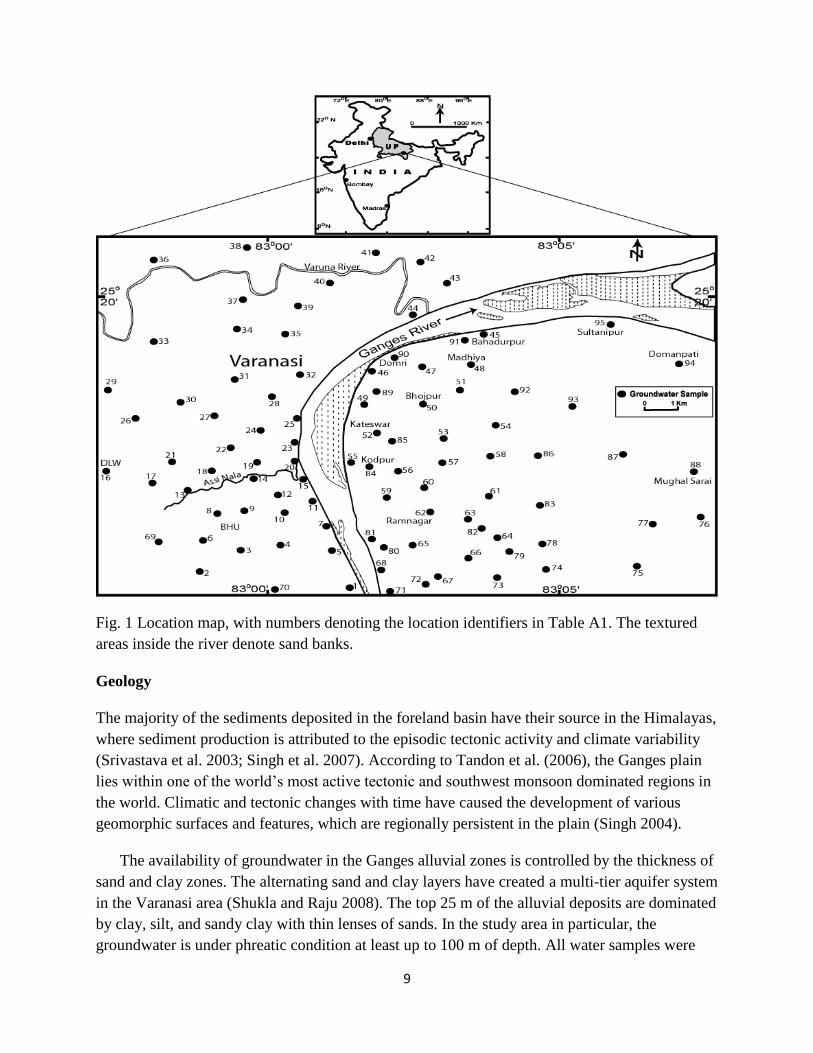
The Ganges River is the major stream in Varanasi, draining the west side of the city and flowing
from south to north (Fig. 1), eventually reaching the Bengal Bay roughly to the southeast. The
city of Varanasi is in the middle part of the Indo-Gangetic plain at an average height of 76.2 m
above the mean sea level with even topography which lies between the peninsular India and the
Siwalik range which represents alluvial deposits filling the Himalayan foreland.
9
Fig. 1 Location map, with numbers denoting the location identifiers in Table A1. The textured
areas inside the river denote sand banks.
Geology
The majority of the sediments deposited in the foreland basin have their source in the Himalayas,
where sediment production is attributed to the episodic tectonic activity and climate variability
(Srivastava et al. 2003; Singh et al. 2007). According to Tandon et al. (2006), the Ganges plain
lies within one of the world’s most active tectonic and southwest monsoon dominated regions in
the world. Climatic and tectonic changes with time have caused the development of various
geomorphic surfaces and features, which are regionally persistent in the plain (Singh 2004).
The availability of groundwater in the Ganges alluvial zones is controlled by the thickness of
sand and clay zones. The alternating sand and clay layers have created a multi-tier aquifer system
in the Varanasi area (Shukla and Raju 2008). The top 25 m of the alluvial deposits are dominated
by clay, silt, and sandy clay with thin lenses of sands. In the study area in particular, the
groundwater is under phreatic condition at least up to 100 m of depth. All water samples were

10
taken from depths shallower than 100 m. Depth of water level varies between 5 and 29 m below
ground level. The water level shows lowering trends in some parts of the study area because of
fast urbanization and intensive pumping for domestic and irrigation use. Groundwater is
extracted through dug wells, hand tube wells and deep bore wells. Dug wells and shallow tube
wells (hand pumps) mainly tap the unconfined aquifers. General depth of hand tube wells and
deep bore wells ranges 60−70 m and 80−250 m below ground level, respectively, and at the
deeper levels aquifer occurs in semi-confined to confined conditions.
Arsenic contaminated aquifers are pervasive throughout the entire Ganges River basin
(Chakraborti et al. 2003; Srivastava et al. 2003; Acharyya 2005; Tandon et al. 2006; Singh et al.
2007; Chauhan et al. 2009; Kumar et al. 2010; Shah 2010; Raju 2012; Srivastava and Sharma
2013; Saha and Shukla 2013; Chandana et al. 2015; Singh et al. 2016; Kumar et al. 2016).
Geomorphological controls, such as the meandering pattern of the Ganges and Brahmaputra
River, is responsible for the localized depositions of arsenic rich sediments along the course of
the river. Consequently, groundwater arsenic contamination is not uniformly found in the Ganges
plain, but is present in pockets along different states of India (Charkraborti et al. 2003).
According to McArthur et al. (2001), high concentrations of arsenic are restricted to Holocene
sediments rich in organic matter resulting in a reducing environment. High concentrations of iron
also seem to play a role in releasing arsenic from minerals in the sediments. Arsenic is adsorbed
by iron oxides, which form a part of fine grained sediments. These sediments are rapidly reduced
because the rich organic matter consumes oxygen. Release of arsenic into the groundwater takes
place after a series of geochemical reactions.
Laboratory analysis
A total of 95 groundwater samples from dug wells, hand pumps, and deep bore wells (Fig. 1) in
the study area were collected during May 2007 (samples 1-68) and in May 2012 (samples 69-95)
and analyzed to understand chemical variations in groundwater quality. The results are listed in
the Appendix. Concentrations are reported in mg/L, that is, in units of mass per volume, which is
only approximately equal but not exactly the same as the dimensionless part per million (ppm)
given that the mass of one liter is not exactly equal to one kilogram because the groundwater
density varies with fluctuations in ion concentrations. The arsenic and iron concentrations are
reported in g/L to have larger values.
Samples collected were filtered using 0.45 µm pore size membrane and stored in
polyethylene bottles which are initially washed with 10% HNO3 and rinsed thoroughly three
times with distilled water. A duplicate set of samples was collected and acidified to 2pH by
adding ultra-pure concentrated HNO3 for heavy metal measurements. Physico-chemical
characteristics of groundwater samples were determined using standard analytical methods (Rice
et al. 2012). Physical parameters like pH and electrical conductivity were measured with portable
ion meters (Elico Model). Total hardness and calcium were estimated by EDTA titrimetric

11
method, and magnesium estimated by the difference of the hardness and calcium. Total
alkalinity, carbonate and bicarbonate as well as chloride were estimated by titrimetric method.
Sodium and potassium were estimated by flame photometer (Elico Model CL-378). Sulfate
estimations were done by the gravimetric method. Nitrate and iron were analyzed by the UV-
spectrophotometer (Lab India Model UV 3000). Fluoride was measured using an ion analyzer
(Orion Model 4 star) with an ion selective electrode. Total arsenic in groundwater was
determined by flow-injection-hydride generation atomic absorption spectrometry (FI-HG-AAS)
(Perkin Elmer). The accuracy of the analytical method using FI-HG-AAS was verified for
arsenic by analyzing Standard Reference Materials from Environmental Monitoring and Support
Laboratory of the U. S. Environmental Protection Agency, Cincinnati, OH, USA. The analytical
precision for the measurement was determined by calculating the ionic balance error, which is
generally found to be within ±5%. Ion speciation in groundwater was calculated using computer
code WATEQ4F program (Ball and Nordstrom 1992). In this publication, the interest was
restricted to the mapping of the concentration of iron and arsenic, considering the effect of the
rest of the ions but disregarding the rest of the non-compositional measurements, such as pH and
electrical conductivity.
The partition matrix
As explained above, the data need to be pre-processed before applying geostatistics and the
results in terms of the pre-processed balances need to be backtransformed. Here, to facilitate the
understanding, we illustrate those steps numerically just for one location before going into the
massive generation of maps covering the entire area of interest. The very first step in the pre-
processing is the preparation of the partition matrix, which remain the same during the entire
study.
There are 11 measured parts in this case (Table A1): Fe ( iz s1 ), As ( iz s2 ), Ca ( iz s3 ), Mg
( iz s4 ), Na ( iz s5 ), K ( iz s6 ), HCO3 ( iz s7 ), SO4 ( iz s8 ), Cl ( iz s9 ), NO3 ( iz s10 ) and F
( iz s11 ). As the interest is restricted to the mapping of the first two parts, Fe and As, it is not
necessary to define the entire partition matrix, which we decided to be:

12
00
00
00
00
00
00
00
00
00000000011
11111111111
Θ , (9)
where the dots denote unspecified values. Consequently, according to Eq. 3, the first two
balances are:
21
21
91
111098765431
)(
)(ln
29
29
ii
iiiiiiiiii
zz
zzzzzzzzzb
ss
ssssssssss
, (10)
i
ii
z
zb
s
ss
2
12 ln
11
11
. (11)
Note that, because of the form of the first balance, although we are not interested in mapping
ions other than Fe and As, the transformations still use information from the additional nine ions,
thus the logratios depend on all 11 ions. For the first well (Table A1), the concentrations are
285.0Fe mg/L, 0.0023As mg/L and for the other ions 62, 31.3, 13.9, 3.6, 334, 10, 35, 7.3,
0.89 mg/L. Hence
24511.8)0023.0285.0(
)89.03.735103346.39.133.3162(ln
29
29
21
91
11
sb , (12)
40796.30023.0
285.0ln
11
1112
sb . (13)
The contrast matrix
For the case of the partition matrix in Eq. 9, the 11 by 10 contrast matrix is

13
00
00
00111
1
111
1
929
2
929
2
922
9
922
9
Ψ . (14)
For estimated balances isb* , the backtransformed, estimated parts are
i
i
ii
b
b
c
s
s
ssz
*
2
*
1
**
0929
2
0929
2
00111
1
922
9
00111
1
922
9
exp . (15)
Considering that we are interested only in iz s*
1 and iz s*
2 , we set to 0 all estimated balances
from ib s*
3 to ib s*
11 , which is equivalent to projecting the composition into a two dimensional
subspace, thus ignoring 9 coordinate-balances:
iii bbcz ssss
*
2
*
11
*
1111
1
922
9exp (16)
iii bbcz ssss
*
2
*
11
*
2111
1
922
9exp (17)
Given that, in addition, the sum of all parts in this case does not add up to a constant value, it is
necessary to use Eq. 8 to recover the original units in mg/L. Because the interest is in mapping
Fe and As, Eq. 8 turns into
2
*T
1
*T
*
1211*
expexp ii
i
zzc
sbΨsbΨ
sss
, (18)
where, again, the asterisks denote estimated values. Let us assume that 24511.81
*
1 sb ,
40796.31
*
2 sb and 2873.0*
1211 ss zz . By Eq. 16 and 17:

14
057022.0*
1
*
1 icz ss (19)
00046.0*
1
*
2 icz ss . (20)
Scaling by Eq. 18
285.0057022.000046.0057022.0
2873.01
*
1
sz (21)
0023.000046.000046.0057022.0
2873.01
*
2
sz (22)
we obtain the estimated values in mg/L of Fe and As, respectively. Note that these two
concentrations are exactly the same values used to calculate the balances. This result is obtained
because there is always a bijection between the original space of the parts and that of the
logratios.
Preparation of the maps
Fig. 2 displays the data for the elements of main interest: iron and arsenic. It can be seen that the
distributions are right skewed. Note that the summary statistics in Fig. 2 include a
“compositional mean”. One of the many peculiarities of compositional data is that the straight
calculation of most moments from the data is invalid, but is valid for all quantiles. For most
moments, the coherent values are those calculated based on the logratio transformations and then
backtransformed. Unfortunately, the operation is not always possible, the variance being one
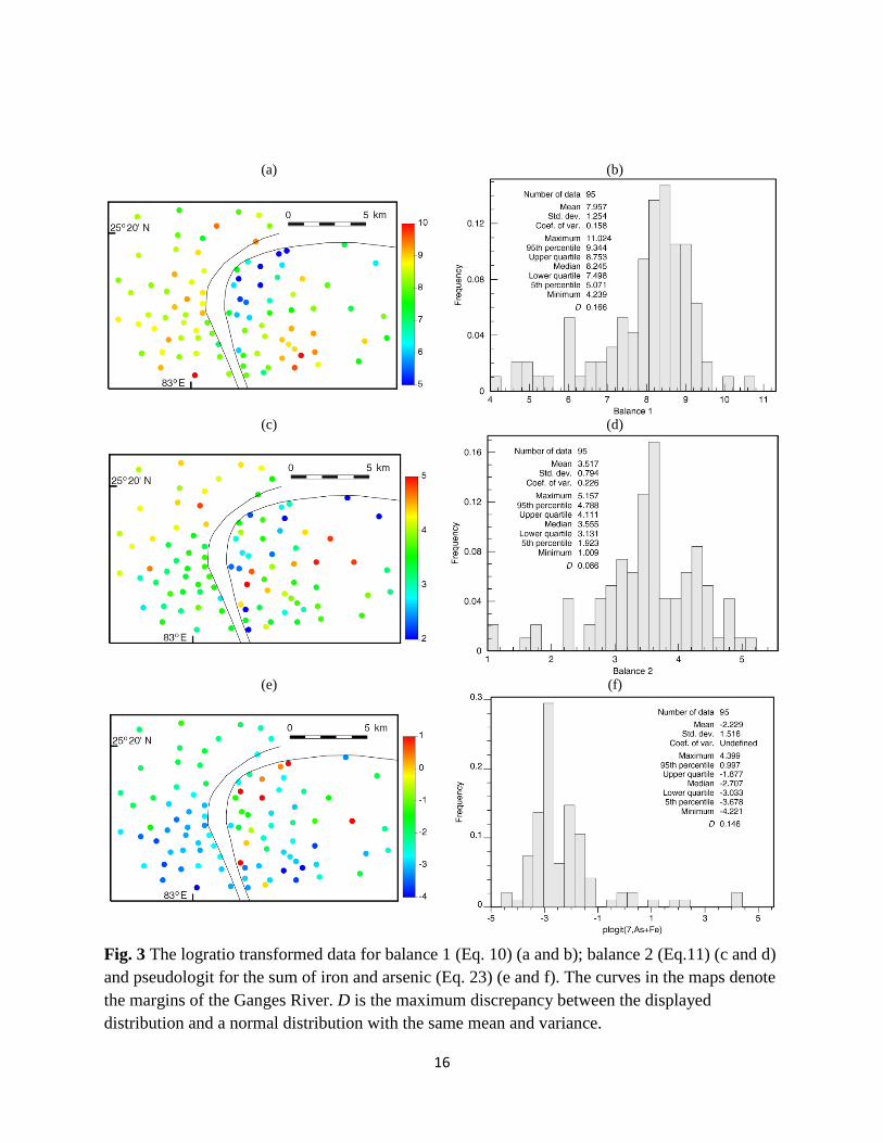
case. For example, from Fig. 3, the mean values for the logratio transformations are (7.957,
3.517, −2.229). The backtransformed values using Equations (18), (19) and (20), 675.6 and 4.7
g/L, here called compositional mean, are the values for the mean concentration of Fe and As,
not those calculated directly as arithmetic means of the observations, which are (1000.5, 9.3).
The geometric mean is one of the few moments that can be calculated directly from the data, thus
its popularity among compositional analysts, but not necessarily among earth scientist.
Consequently, we list both.

15
(a)
(b)
(c)
(d)
Fig. 2 Display of well data for iron (a and b) and arsenic (c and d). Posting of values is in
logarithmic scale, with the curves denoting the margins of the Ganges River.
Because we will use Eq. 18 for the backtransformation of the balances, we need to prepare an
estimate of the sum of iron plus arsenic, which also requires a logratio transformation, for which
we have selected the following pseudologit:
.lnplogit1211
1211
ss
sss
zzp
zzi
(23)
In a logit, parameter p is the maximum possible value for the variable in the denominator. Here
instead, we have taken 0.7p , which is a value close but larger than the maximum value of
6.915 mg/L in the sample (well 81, Table A1). Fig. 3 shows the two balances and the
pseudologit.
16
(a)
(b)
(c)
(d)
(e)
(f)
Fig. 3 The logratio transformed data for balance 1 (Eq. 10) (a and b); balance 2 (Eq.11) (c and d)
and pseudologit for the sum of iron and arsenic (Eq. 23) (e and f). The curves in the maps denote
the margins of the Ganges River. D is the maximum discrepancy between the displayed
distribution and a normal distribution with the same mean and variance.

17
Calculation of the logratio transformations marks the end of the data preparation necessary
for the adequate application of geostatistics.
The interest in our case is in sequential Gaussian simulation, which, as we have seen,
requires not only that the data can vary from to + , but also that the univariate
distributions be normal, which is hardly the case here, perhaps with the sole exception of balance
2 in Fig. 3. Hence, normal score transformations are in order. Note that, because normal scores
will be used in the modeling instead of the pseudologit, given that both types of transformations
are monotonous, the normal score transformation is the same regardless of the value selected for
parameter p.
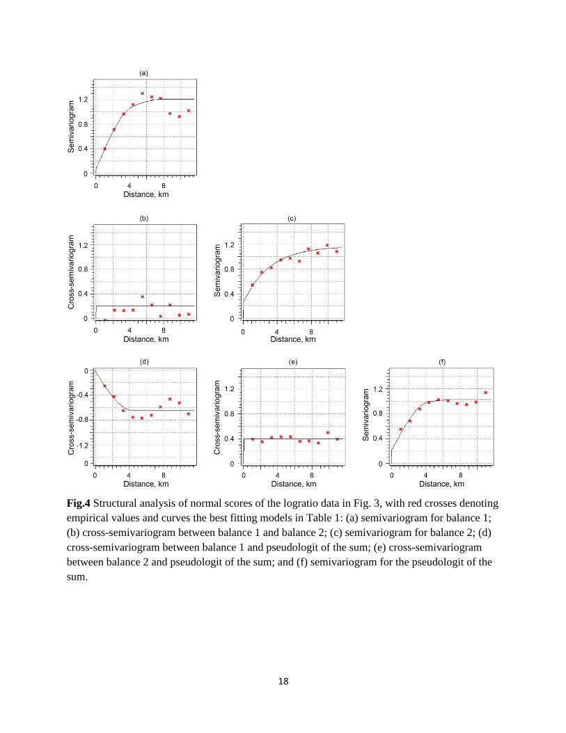
The next step according to the sequential Gaussian simulation procedure in the Geostatistics
Section is the structural analysis, which did not find any significant anisotropies. Fig. 4 and
Table 1 show that all cross-semivariograms follow pure nugget effect models, except for the
cross-semivariogram between the normal scores of balance 1 and of the pseudologit for the sum
of the concentrations of arsenic and iron. Hence, balance 2 should be modeled applying
sequential Gaussian simulation because their normal scores are not spatially correlated to the
normal scores of the other two logratios. The mapping of the other two variables will benefit
with the use of sequential Gaussian cosimulation, although marginally because the data are all
collocated.
18
Fig.4 Structural analysis of normal scores of the logratio data in Fig. 3, with red crosses denoting
empirical values and curves the best fitting models in Table 1: (a) semivariogram for balance 1;
(b) cross-semivariogram between balance 1 and balance 2; (c) semivariogram for balance 2; (d)
cross-semivariogram between balance 1 and pseudologit of the sum; (e) cross-semivariogram
between balance 2 and pseudologit of the sum; and (f) semivariogram for the pseudologit of the
sum.

19
Table 1 Parameters for the models best fitting to the empirical values in Fig. 4. S−N denotes sill
minus nugget, R the range, the root bal denotes balance, exponent. is the abbreviation for
exponential, and plogit for pseudologit.
Variable(s) Nugget Type S−N R, km Type S−N R, km
bal1 0.06 spherical 0.7 4.4 spherical 0.45 8.0
bal1-bal2 0.2
bal1-plogit −0.02 spherical −0.63 4.4
bal2 0.25 exponent. 0.92 9.2
bal2-plogit 0.4
plogit 0.2 spherical 0.68 4.4 spherical 0.15 8.0
In this study, it is sufficient to limit the number of realizations to 100 per variable to properly
cover the uncertainty space, that is, a total of 300 realizations. Space restrictions do not allow
display of all 300 realizations. Under the circumstances, we have arbitrarily limited the rendition
to the first realization for each one of the logratios, which appear in Fig. 5. The mapping is
completed by backtransforming each one of the 100 triplets of realizations.

20
(a)
(b)
(c)
Fig. 5 Logratio maps, with the white curves marking the Ganges River margins: (a) balance 1;
(b) balance 2; and (c) pseudologit for the sum of arsenic and iron concentrations.
Figs. 6 and 7 show the results for three realizations, this time properly selected to allow an
appreciation of the degree of uncertainty in the results. These are conditional realizations, so they
honor the values at all 95 wells (Figs. 1a and 1c) and have the same style of spatial fluctuation to
the degree that such fluctuation can be captured by the semivariograms and cross-
semivariograms in Fig. 4. The realizations are obtained by repeating node by node the same type

21
of calculations in Eqs. 16−22, starting with the nodal values displayed in Fig. 5 and continuing
with the remainder 99 realizations per variable. The fourth map in Figs. 6 and 7 is a filtered map
of spatial fluctuation, maps that still honor the data but not the semivariograms and cross-
semivariograms anymore. For each attribute, the realizations and the filtered map cover both
realms of underlying and general style of fluctuation. Most likely, none of the realizations is the
exact depiction of the underlying map, but collectively should help the reader to figure out the
values that the attributes can take at those locations not considered in a sample of only 95
observations per attribute in an area of roughly 210 km2. The filtered map is an average map of
all realizations, thus summarizing in one map all possibilities. The filtered version, while unique,
is biased, because it provides a false rendition of the degree of complexity in the geographical
variations of the attribute. Conceptually, a filtered map is the same map that would be obtained
by (co)kriging the data instead of generating the (co)simulations. In that sense, stochastic
simulation is a superior tool to kriging because it allows portraying both the actual fluctuations
plus the map resulting from removing the high frequency components. Figs. 6d and 7d are
simply a map of the compositional mean node by node, which are minimum mean square error
estimates for the concentrations at those nodes (Remy et al. 2009).

22
(a)
(b)
(c)
(d)
Fig. 6 Arsenic maps, with the white lines displaying the margins of the Ganges River: (a)
realization with the 5th lowest average concentration (3.84 g/L); (b) realization with median
concentration (4.72 g/L); (c) realization with the 5th largest average concentration (5.47 g/L);
(d) filtered map of concentration showing the general spatial trend.

23
(a)
(b)
(c)
(d)
Fig. 7 Iron maps, with the white curves showing the Ganges River margins. Maps (a−c) are for
the corresponding realization in Figs. 6a−6c, which have different ranks in terms of the
percentiles for the average concentrations. (d) is the filtered map for iron concentration.
Map comparisons do not necessarily have to be done among a few realizations and done
visually. The same probability distributions for every node that were used to calculate nodal
means displayed as filtered maps can be used for other purposes, such as counting the proportion
of values per node below or above certain thresholds. So, for example, if at node is the
concentration of Fe iz s1 is higher than 800 g/L for 32% of the values at the node, then we
can estimate 32.0800Prob 1 iz s , estimation that can be easily done and without resorting
to any mathematical assumptions. Nothing prevents from expanding the comparison to more
than one concentration by applying the same Eq. 1 behind sequential Gaussian simulation. For
example, it is possible to calculate the joint probability that 800: FeA and 10: AsB . Fig. 8
displays the results for the univariate and multivariate probabilities after carrying out the
calculations for all nodes. Why 800 g/L and 10 g/L? Because in this case the interest was to
show the areas in which both elements were high. The value of 10 g/L for As was taken directly
from the critical value established by WHO. As for the 800 g/L for Fe, it was a value in the
moderately high range of observed values (Fig. 2b). Taking another moderately high value, the
results would have been different, but not by much.

24
(a)
(b)
Fig. 8 Probability maps, with the white curves marking the margins of the Ganges River: (a)
probability that the iron concentration is higher than 800 g/L; (b) probability that the iron
concentration is higher than 800 g/L and at the same time that of arsenic is higher than 10 g/L.
Discussion
According to Fig. 7, iron concentration in the groundwater of the study area is above 300 g/L in
most of the study area except primarily towards the southwest. Varanasi is on the concave side
(erosional part) of a long meander (Fig. 1). The high arsenic concentrations should be expected
on the convex side (depositional part) of the Ganges River (Fig. 6), higher in organic material
(McArthur et al. 2001). Fig 8b indicates that simultaneous occurrence of high values for both
iron and arsenic is restricted to two anomalies on the right margin of the river, where Fe-
oxyhydroxide coated sediment grains have been reported preferentially entrapped in more recent
Holocene alluvial argillaceous sediments in entrenched channels and flood plains (Raju 2012).
High concentrations of iron in north Varanasi are not associated with high concentrations of
arsenic, most likely because of scarcer availability of organic matter. The sources of arsenic, iron
and organic material are all natural, not of anthropogenic origin.
Varanasi is one of the oldest continuously occupied cities in the world that started and grew
for millennia in the left banks of the Ganges River (Khan et al. 1988; Kayastha and Mohan
2000). Despite lack of technology only recently available, it looks like the ancient residents of
Varanasi always knew that there was something unhealthy in the groundwater at the other side of
the river that did not invite them to expand the city toward the east. Today, with the urban
development at places like Ramnagar, Bhojpur, Kodpur, Kateswar, Domri, Madhiya,
Bahadurpur, Sultanipur and Domanpati the populations at those communities are the ones that
have the highest risks of developing health problems should they consume groundwater from
local wells because of levels of As concentration above the 10 ppb—roughly equal to 10 g/L—
established as the highest safe limit by WHO.

25
Conclusions
Combined use of compositional data analysis and geostatistics allows to adequately preparing
maps of continuous variations of hydrochemical attributes only partially known at the few
locations where specimens have been taken for analysis. Their combined application provides
for: (a) preparing realization maps honoring the data and the style of fluctuation—spatial
correlation—implicit in the same data; (b) displaying one filtered map per attribute of interest
showing only the low frequency fluctuations; and (c) reporting joint fluctuation of two of more
attributes with their associated uncertainty.
Application of the methodology to reported values for 11 ions at 95 water wells in an area of
about 210 km2 indicates that groundwater concentrations of arsenic at the city of Varanasi are
significantly below the 10 ppb recommended by the WHO. In contrast, a crescent of about 50
km2 underneath the Ganges and along the depositional side of the river meander east of Varanasi
has levels of arsenic of natural origin in the groundwater that are above the maximum level
recommended by WHO. Hence, public health authorities should prevent the consumption of
groundwater from wells in all areas with high arsenic levels.
The mathematics in the methodology is completely general, not depending on the
geochemical nature of the attributes. Hence, the study here can be used as a guide for the
hydrochemical mapping of elements and ions in other places.
Acknowledgments
This paper completed a mandatory internal review by the U.S. Geological Survey (USGS) before
final submission to the journal (http://pubs.usgs.gov/circ/1367/). We wish to thank Tanya
Gallegos (USGS) and Josep Martín-Fernández (University of Girona) for suggestions that helped
improving the manuscript.
SR/S4/ES-160/2005has been supported by the Department of Science and Technology
(DST), New Delhi, under research project “SERC” (SR/S4/ES-160/2005) during 2006-2008.
J.J. Egozcue and V. Pawlowsky-Glahn have been supported by the Spanish Ministry of
Education and Science under projects ‘CODA-RETOS’ (Ref. MTM2015-65016-C2-1-R
MINECO/FEDER.UE) and ‘COSDA’ (Ref. 2014SGR551); and by the Agència de Gestió
d'Ajuts Universitaris i de Recerca of the Generalitat de Catalunya.

26
References
Acharyya SK (2005) Arsenic levels in groundwater from Quaternary alluvium in Ganga plain
and the Bengal Basin, Indian Subcontinent: Insights into influence of stratigraphy. Gondwana
Research 8(1):55−66
Aitchison J (2003) The statistical analysis of compositional data. The Blackburn Press, Caldwell,
NJ, reprint of 1986 edition plus 19 pages of new text, 435 pp
Aitchison J, Egozcue JJ (2005) Compositional data analysis: where are we and where should we
be heading? Mathematical Geology 37(7):829−850
Ball JW, Nordstrom DK (1992) User’s manual for WATEQ4F with revised thermodynamic
database and test cases for calculating speciation of minor, trace and redox elements in
natural waters. U.S. Geological Survey Open File Report 91-183, 189 pp
British Geological Survey (BGS) (2001) Arsenic contamination of groundwater in Bangladesh.
Technical report, BGS, Department of Public Health Engineering (Bangladesh), Report
WC/00/019, 630 pp, http://www.bgs.ac.uk/arsenic/Bangladesh/
Caers J (2011) Modeling Uncertainty in the Earth Sciences. Wiley-Blackwell, Chichester, UK,
229 pp
Chakraborti D, Mukherjee SC, Pati S, Sengupta MK, Rahman MM, Chowdhury UK, Lodh D,
Chanda CR, Chakraborti AK, Basu GK (2003) Arsenic groundwater contamination in Middle
Ganga Plain, Bihar, India: A future danger? Environmental Health Perspectives 111(9):
1194−1201
Chandana M, Enmark G, Nordborg D, Sracek O, Nath B, Nickson RT, Herbert R, Jacks G,
Mukherjee A, Ramanathan AL, Choudhury R, Bhattacharya P (2015) Hydrogeochemical
controls on mobilization of arsenic in groundwater of a part of Brahmaputra River flood
plain, India. Journal of Hydrology: Regional Studies, 4:154−171
Chauhan VS, Nickson RT, Chauhan D, Iyengar L, Sankararamakrishnan N (2009) Ground water
geochemistry of Ballia district, Uttar Pradesh, India and mechanism of arsenic release.
Chemosphere 75(1):83−91
Chilès JP, Delfiner P (2012) Geostatistics: Modeling spatial uncertainty. John Wiley & Sons,
Inc., Hoboken, NJ, second edition, 734 pp
Egozcue JJ (2009) Reply to "On the Harker variation diagrams;..." by J. A. Cortés. Mathematical
Geosciences 41(7):829−834
Egozcue JJ, Pawlowsky-Glahn V (2005) Groups of parts and their balances in compositional
data analysis. Mathematical Geology 37(7):795−828
Egozcue JJ, Pawlowsky-Glahn V (2006) Simplicial geometry for compositional data. In:
Buccianti A, Mateu-Figueras G, Pawlowsky-Glahn V, editors, Compositional data analysis in
the geosciences: From theory to practice. Geological Society Special Publication No. 264,
London, 145−159

27
Egozcue JJ, Pawlowsky-Glahn V (2011) Basic concepts and procedures. In: Pawlowsky-Glahn
V, Buccianti A, editors, Compositional data analysis: Theory and applications. John Wiley &
Sons, Chichester, UK, 12−28
Egozcue JJ, Pawlowsky-Glahn V, Mateu-Figueras G, Barceló-Vidal C (2003) Isometric logratio
transformations for compositional data analysis. Mathematical Geology 35(3):279−300
Emery X (2004) Testing the correctness of the sequential algorithm for simulating Gaussian
random fields. Stochastic Environmental Research and Risk Assessment 18(6):401−413
Greenacre M (2011) Measuring subcompositional incoherence. Mathematical Geosciences
43(6):681−693
Hogg RV, McKean J, Craig AT (2012) Introduction to mathematical statistics. Pearson
Education Ltd., Harlow, UK, 7th edition, 649 pp
Isaacs EH, Srivastava RM (1989) An introduction to applied geostatistics. Oxford University
Press, New York, 561 pp
Kayastha SL, Mohan A (2000) Varanasi: An ancient city of continuity and culture. Proceedings
of the National Symposium Milestones in Petrology at the end of the Millennium and Future
Perspectives, Department of Geology, Banaras Hindu University, Varanasi, pp. 20−29
Khan AA, Nawami PC, Srivastava MC (1988) Geomorphological evolution of the area around
Varanasi, UP with the aid of aerial photographs and LANDSAT imageries. Geological
Survey of India Rec. 113: 31−39
Kumar M, Kumar P, Ramanathan AL, Bhattacharya P, Thunvik R, Singh UK, Tsujimura M,
Sracek O (2010) Arsenic enrichment in groundwater in the middle Gangetic Plain of Ghazipur
District in Uttar Pradesh, India. Journal of Geochemical Exploration 105(3):83−94
Kumar M, Rahman MM, Ramanathan AL, Naidu R (2016) Arsenic and other elements in
drinking water and dietary components from the middle Gangetic plain of Bihar, India:
Health risk index. Science of Total Environment 539:125−134
McArthur JM, Ravenscroft P, Safiulla S, Thirlwall MF (2001) Arsenic in groundwater: testing
pollution mechanism for sedimentary aquifers in Bangladesh. Water Resources Research
37(1):109−117
Meyzonnat G, Larocque M, Barbecot F, Pinti DL, Gagné S (2016) The potential of major ion
chemistry to assess groundwater vulnerability of a regional aquifer in southern Quebec
(Canada). Environmental Earth Sciences 75(1): article 68, 12 pp
Olea RA (2006) A six-step practical approach to semivariogram modeling. Stochastic
Environmental Research and Risk Assessment 39(5):453−467
Olea, RA (2009) A Practical Primer on Geostatistics: U.S. Geological Survey, Open-File Report
2009-1103, 346 pp, http://pubs.usgs.gov/of/2009/1103

28
Palarea-Albaladejo J, Martín-Fernández JA (2015) zCompositions—R package for multivariate
imputation of left-censored data under a compositional approach. Chemometrics and
Intelligent Laboratory Systems, 143:85−96
Pawlowsky-Glahn V, Egozcue JJ (2001) Geometric approach to statistical analysis on the
simplex. Stochastic Environmental Research and Risk Assessment 15(5):384−398
Pawlowsky-Glahn V, Egozcue JJ (2016) Spatial analysis of compositional data: A historical
review. Journal of Geochemical Exploration 164:28−32
Pawlowsky-Glahn V, Egozcue JJ, Lovell D (2015a) Tools for compositional data with a total.
Statistical Modelling 15(2):175−190
Pawlowsky-Glahn V, Egozcue JJ, Olea RA, Pardo-Igúzquiza E (2015b) Cokriging of
compositional balances including a dimension reduction and retrieval of original units.
Journal of the Southern African Institute of Mining and Metallurgy 115(1):59−72
Pawlowsky-Glahn V, Egozcue JJ, Tolosana-Delgado R (2015c) Modeling and analysis of
compositional data. John Wiley & Sons Ltd, Chichester, UK, 247 pp
Pyrcz MJ, Deutsch CV (2014) Geostatistical reservoir modeling. New York, Oxford University
Press, second edition, 433 pp
Raju, NJ (2012) Arsenic exposure through groundwater in the middle Ganga plain in the
Varanasi environs, India: A future threat. Journal of the Geological Society of India
79:302−314
Remy N, Boucher A, Wu J (2009) Applied geostatistics with SGeMS—a user’s guide.
Cambridge University Press, Cambridge, UK, 264 pp
Rice EW, Baird RB, Eaton AD, Clesceri LS, editors (2012) Standard methods for the
examination of water and wastewater. American Public Health Association, American Water
Works Association, Water Environment Federation, Washington, DC,
https://www.standardmethods.org/
Saha D, Shukla RR (2013) Genesis of arsenic rich groundwater and the search for alternative
safe aquifers in the Gangetic plain, India. Water Environmental Research 85(12):2254−2264
Sha ZUH, Ahmad Z (2015) Hydrochemical mapping of the Upper Thal Doab (Pakistan) using
the geographical information system. Environmental Earth Sciences 74(3):2757−2773
Shah BA (2010) Arsenic contaminated groundwater in Holocene sediments form part of middle
Ganga plain, Uttar Pradesh, India. Current Science 98(10):1359−1365
Shukla UK, Raju NJ (2008) Migration of the Ganga River and its implications on hydro-
geological potential of Varanasi area, U.P., India. Journal of Earth System Science
117(4):489−498
Singh IB (2004) Late Quaternary history of the Gangetic plain. Journal of the Geological Society
of India 64:431−454

29
Singh M, Singh IB, Muller G (2007) Sediment characteristics and transportation dynamics of the
Ganga River. Geomorphology 86(1−2):144−175
Singh S, Raju NJ, Gossel W, Wycisk P (2016) Assessment of pollution potential of leachate
from the municipal solid waste disposal site and its impact on groundwater quality, Varanasi
environs, India. Arabian Journal of Geosciences 9(2): article 131, 12 pp
Srivastava P, Singh IB, Sharma M, Singhvi AK (2003) Luminescence chronometry and Late
Quaternary geomorphic history of the Ganga Plain, India. Paleaogeography,
Paleaoclimatology, Paleaoecology 197(1−2):15−41
Srivastava S, Sharma YK (2013) Arsenic occurrence and accumulation in soil and water of
eastern districts of Uttar Pradesh, India. Environmental Monitoring and Assessment
185(6):4995−5002
Tandon SK, Gibling MR, Sinha R, Singh V, Ghazanfari P, Dasgupta A, Jain M, Jain V (2006)
Alluvial valleys of the Ganga Plains, India: Timing and causes of incision. In: Dalrymple
RW, Lickie DA, Tillman RW, editors, Incised valleys in time and space. Society for
Sedimentary Geology (SEPM) Special Publications 85, Tulsa, OK, 15−35
Verly G (1993) Sequential Gaussian cosimulation: A simulation method integrating several types
of information. In: Soares, A, editor, Geostatistics Troia’92. Kluwer Academic Publishers,
Dordrecht, The Netherlands, vol. 1:543–552
Webster R, Oliver MA (2015) Basic steps in geostatistics: The variogram and kriging. Springer,
Heidelberg, 100 pp
World Health Organization (WHO) (2011) Arsenic in drinking water, 16 pp,
http://www.who.int/water_sanitation_health/dwq/chemicals/arsenic.pdf

30
Appendix
Table A1. Results of laboratory analyses for 11 ions. WT stands for water table, DW for dug
well, HTW for hand tube well, DBW deep borewell
No. Location Source WT m
Fe
g/L
As
g/L
Ca mg/L
Mg mg/L
Na mg/L
K mg/L
HCO3 mg/L
SO4 mg/L
Cl mg/L
NO3 mg/L
F mg/L
1 Malabia HTW -- 285 2.3 62 31.3 13.9 3.6 334 10 35 7.3 0.89
2 Hyd. Gate-BHU HTW -- 209 1.3 76 18.9 131 1.8 320 20 48 9.1 0.67
3 Agri.farm-BHU HTW -- 230 2.8 16 58 19.5 2.6 286 30 26 6 0.75
4 Chittupur HTW -- 415 1.9 100 60.8 47 2.8 318 121 120 1.1 0.48
5 Madarwa DW 14.5 336 2.2 46 40.2 17 4.4 322 5 46 5.7 0.59
6 Jagainpur DW 20 174 2.1 82 14 37.7 3.2 318 15 63 6.6 0.55
7 Samneghat HTW -- 409 9 42 41.9 15.1 2.9 268 12 39 7.5 0.39
8 Karaundi DW 11.6 321 1.8 70 127 111 2.7 510 180 198 0.82 0.82
9 IMS (BHU) HTW -- 319 2.5 20 65 29.9 2.7 286 70 40 6.8 0.86
10 Bhagavanpur DW 8.9 282 3 24 59 52.7 3.8 364 30 55 4.5 0.65
11 Nagwa Chungi HTW 10 414 2.7 20 56.1 33.8 3.4 318 15 53 6.8 0.95
12 Lanka DW 7.2 346 2 3 22 105 86 2.4 382 150 128 1.2 0.88
13 Sunderpur HTW -- 175 1.9 36 65.2 64.8 2.3 404 10 93 1.3 0.77
14 Saketnagar HTW -- 281 2.4 46 62.7 33 3 342 60 74 1.8 0.85
15 Nagwa DW -- 424 2.5 52 48.6 41.4 6.2 302 5 50 3.1 0.56
16 Bhulanpur DW -- 383 1.1 52 50.9 20 3 350 10 35 35 0.8
17 Bikharipur DW 7.6 207 3.2 58 45.6 58 2.3 360 30 98 6.8 0.63
18 Sarainand. DW 11.8 255 2.9 18 48.5 68 3 304 30 80 3.4 0.51
19 Ravindrap. HTW -- 282 2.1 80 22.4 25.4 2.6 264 30 60 2.5 0.49
20 Assighat DW 2.4 255 1.5 48 56.6 74.9 4.3 370 60 95 2 0.67
21 Karkarmitha DW -- 1262 1.8 62 49.8 76.5 4.2 145 100 149 90.4 0.46
22 Kheiriya HTW -- 214 2.3 10 119 144 2.7 524 120 163 1.5 0.85
23 Shivala HTW -- 401 2.3 40 41.3 52.5 40 304 75 65 2.7 0.73
24 Belupur HTW -- 286 1.9 36 69.3 108 28 382 120 138 1.2 0.66
25 Sonarpura HTW -- 306 2.9 16 58.4 73.6 53.3 410 50 93 3.7 0.76
26 Sivadaspur DW 11.2 870 2.2 57 43 64.7 7.9 173 30 97 63.6 0.53
27 Koluwaa HTW -- 356 3.3 10 49.8 130 5.1 366 50 99 2.2 0.64
28 Kamachha DW 5.3 441 3.5 40 51.5 94 28.4 386 90 87 3.2 0.73
29 Chandpura HTW -- 730 2.4 52 33 49.5 3 310 20 40 62.4 0.69
30 Manduadi DW 9.8 980 2.2 59 39.2 80.4 4 356 20 79 76 0.31
31 Gurubagh HTW 12 660 1.8 49 70.5 107 6.6 260 100 169 92 0.6
32 Jangambadi DW 1.4 940 1.9 37 50.3 64.5 33 315 100 72 11 1.12
33 Koharpur DW -- 830 2.1 53 65 40 3 332 40 109 55.1 0.54
34 Cant.Railway St HTW 7.4 980 2 55 32 100 2.8 412 40 49 66.7 1.34
35 Sonia Pokhara DW 4.3 890 1 50 32.7 77.6 5.7 235 90 56 36.6 0.94
36 Central Prison DW -- 800 2.7 56 49.1 75.2 4.5 310 70 109 35 0.36
37 Nadeshwar DW -- 800 2.9 76 20 129 8.1 430 60 12 20.4 0.34
38 Rajanhia DW -- 1480 3 39 46.2 59.5 2.6 375 30 39 48.7 0.98
39 Sanskrat Univ. DW 8 1060 2.5 80 8.2 39.6 3.6 310 10 35 9.6 0.55
40 City Railway St. HTW 9.8 730 2 100 92.5 200 6.5 320 120 397 106 0.63
41 Rasulgarh DW 17.2 860 1.9 50 10.8 41.2 2.8 288 20 40 47.7 0.51
42 Kapiladara DW -- 670 1.7 46 41.8 90.2 3 395 20 107 23.1 0.82
43 Kotwara DW 17.3 500 3.5 69 26.1 70.3 3.5 385 10 51 67.1 0.46
44 Rajghat DW 24.1 430 3.2 79 36.6 92 75 340 100 175 92 0.45
45 Bahadurpur HTW 3.1 5319 80 183 15.3 32 2.1 364 100 109 2.7 1.2
46 Domari HTW -- 438 3 105 12.1 25.8 2.4 386 2.5 37 2.1 0.8
47 Ratanpur HTW -- 4065 23 103 22.5 42.1 4.1 447 2.5 45 2.5 0.9
48 Madhiya HTW -- 362 76 107 45.8 31.6 2.1 405 10 115 3.1 1.1
49 Semra HTW 3.7 1382 24 145 29.6 26.8 1.1 343 100 97 2.4 1
50 Bhojpur HTW -- 6866 45 113 30.5 24.5 1.7 447 10 59 2.4 0.5
51 Jalilpur HTW -- 421 11 73 20.8 23.2 2.3 295 2.5 47 5.6 0.7
52 Kateswar HTW -- 1436 31 101 31.9 20.4 0.8 426 2.5 43 5 0.9
53 Bhakhara HTW -- 353 13 71 3.1 45.2 1.7 288 2.5 53 5.4 1.1
54 Nibupur HTW -- 323 3.8 37 86.8 150 7.3 720 2.5 103 11.9 0.8

31
55 Kodupur HTW -- 365 14 107 34.2 97.3 2.2 589 5 79 3.8 1.2
56 Wajidpur HTW -- 2464 3 85 0.4 73.1 2.1 312 2.5 61 4.1 0.9
57 Nathupur HTW -- 526 1.9 79 21.3 34.9 0.7 345 2.5 57 5.8 0.7
58 Nathupur HTW -- 727 1.2 75 8.4 32 0.7 232 2.5 41 3.6 1.3
59 Kutulupur HTW -- 3527 2.4 123 93.5 69.2 18.2 572 30 225 44.7 0.8
60 Sultanpur DW 3.5 492 2.8 75 35.6 123 1.2 378 10 157 16.1 1.2
61 Mannapur DW -- 450 2.9 68 64 252 23.1 694 10 277 21.9 0.9
62 Kabirpur HTW -- 835 1.6 25 44.6 235 1.6 682 20 111 11.2 0.7
63 Dariyapur DW -- 355 1.1 59 47.3 102 2.5 537 10 85 10.4 0.45
64 Parawara DW -- 329 1.8 81 46.5 114 9.8 502 5 163 6.2 0.5
65 Bhiti HTW -- 320 3 73 25.6 83.2 0.7 325 100 79 6.24 0.6
66 Dahiya DW -- 100 1.9 53 50.2 87.3 1.1 416 2.5 83 5.4 0.9
67 Tangara DW -- 360 2.9 11 50.2 180 1.3 547 2.5 109 11.9 0.8
68 Rathupur HTW -- 346 2.7 59 20.5 35.7 0.6 294 10 29 8.7 0.9
69 Pongalpur HTW -- 400 9 97 13.5 281 1.5 568 45.4 262 22.4 0.7
70 Karaya HTW -- 100 1.3 74 44.5 109 109.4 450 30.2 210 70 2
71 Ralhupur HTW 3.5 250 19 84 21.9 156 17 385 34 200 9.2 0.9
72 Tengara DW -- 3390 10 82 68.8 192 1.9 628 60 220 13.2 1
73 Kataria DW -- 170 1.4 60 39.4 123.5 4.2 386 64 120 3.5 1
74 Ekuni DW 4.2 520 2.9 30 41.3 288 6.8 650 53.1 240 1.5 2
75 Chakia HTW -- 1000 6 98 17.1 139 2 293 208 98 9.7 0.4
76 Taranpur DBW -- 500 6 82 22.6 76.3 2.5 326 16 118 3.2 0.5
77 Prasrampur DBW 3.9 300 1.3 70 34 48.2 2.8 311 25.6 82 5.5 1
78 Kamlapur HTW 2.7 350 1.8 62 20.7 124.4 2.7 418 64.5 80 67 2
79 Airi DBW -- 100 1.5 82 32.8 96.9 4.4 433 30.3 98 6 2
80 Bengali DBW 3.4 200 22 58 52.3 80.4 1.7 335 70.6 118 8.9 1
81 Bagheli Tola DW 4.1 6900 15 92 1.3 278 7.9 317 110 280 90 0.5
82 Parorwa HTW -- 380 1.6 106 13.4 95 3.2 410 29.9 124 7 0.8
83 Khajurgaon DBW -- 170 1.4 86 17.8 87 2.3 366 40 88 1.9 1
84 Kodpur HTW -- 980 36 94 4.2 104.4 2.7 365 60 118 4.3 0.4
85 Katesar DBW 2.2 1200 21 110 1.8 27.2 2.2 220 23.9 95 4.7 0.2
86 Shahupuri Col. DW -- 1600 1.5 236 31.72 125 2.9 319 19.2 494 1.9 0.7
87 Chandhasi HTW -- 6000 6.6 138 19.3 200 4.9 518 90.2 207 62.6 2
88 Mughal Sarai HTW -- 700 8 60 26.3 111.6 39 360 57.8 119 13.4 2
89 Semra HTW 6.2 6400 23 162 3.7 48.2 2.2 360 13 148 3 0.2
90 Domri HTW -- 700 30 130 13 88.7 2.8 392 100.5 95 5.9 0.2
91 Bahadurpur HTW 4.9 4000 72 196 5 91.8 13 612 14 135 19 0.2
92 Dhulaipur HTW 5.6 700 1.5 190 35.3 175.1 5.7 657 89.9 247 1.3 0.7
93 Vyasnagar DW 3.6 1300 1.4 260 4.5 93.1 1.4 292 26.4 417 3.3 0.5
94 Domanpati HTW 2.9 900 70 139 20.9 135.8 9.8 571 24.2 123 21.3 0.2
95 Sultanipur HTW 4.1 200 48 82 26.8 68.4 4.6 340 29 102 11.9 0.7