ADVANCED WATER DISTRIBUTION MODELING AND MANAGEMENT 1 Water systems... · 2009-03-12 · ADVANCED WATER DISTRIBUTION MODELING AND MANAGEMENT Authors Thomas M. Walski Donald V. Chase

ADVANCED WATER DISTRIBUTION MODELING

AND MANAGEMENT

Authors

Thomas M. Walski

Donald V. Chase

Dragan A. Savic

Walter Grayman

Stephen Beckwith

Edmundo Koelle

Contributing Authors

Scott Cattran, Rick Hammond, Kevin Laptos, Steven G. Lowry,

Robert F. Mankowski, Stan Plante, John Przybyla, Barbara Schmitz

Peer Review Board

Lee Cesario (Denver Water), Robert M. Clark (U.S. EPA),

Jack Dangermond (ESRI), Allen L. Davis (CH2M Hill),

Paul DeBarry (Borton-Lawson), Frank DeFazio (Franklin G. DeFazio Corp.),

Kevin Finnan (Bristol Babcock), Wayne Hartell (Bentley Systems),

Brian Hoefer (ESRI), Bassam Kassab (Santa Clara Valley Water District),

James W. Male (University of Portland), William M. Richards

(WMR Engineering), Zheng Wu (Bentley Systems ),

and E. Benjamin Wylie (University of Michigan)

Click here to visit the Bentley Institute Press Web page for more information

http://www.bentley.com/en-US/Training/Bentley+Institute+Press.htm

C H A P T E R

9Modeling Customer Systems

Most water distribution system modeling is done by or for water utilities. In someinstances, there are entire water systems that are served by other water utilitiesthrough wholesale agreements, such that the water source is actually the neighboringsystem. This type of situation is shown in Figure 9.1 where the source water utilitydelivers to an adjacent customer water utility through a meter and a backflow preven-ter. Some examples are military bases, prisons, university campuses, and major indus-tries. These systems can include domestic water use, industrial process water, coolingwater, irrigation water use, and fire protection systems. Most water system designwork is the same within a customer’s system as it is within the water utility’s system.

Figure 9.1Customer water system using utility's system as a water source

There are several principal differences between working for a customer water systemand a utility system. When working for a customer water system, the designer doesnot control the source of water, and therefore must model back into the utility system.More information regarding the extent to which the water utility’s system must bemodeled can be found in Chapter 8 (see page 326). In addition, the designer mustaccount for head losses in meters and backflow preventers in the customer water sys-tem, which are usually not an issue for the utility engineer.

Water

Utility

Source MeterBackflowPreventer

Water

System

Customer

M

394 Modeling Customer Systems Chapter 9

9.1 MODELING WATER METERSA customer’s water meter is usually a positive displacement technology meter used onlines sized from 5/8 in. to 2 in., or a turbine technology meter (shown in Figure 9.2)for lines sized 1-1/2 in. to 20 in. For some applications in which the flow rate variesgreatly, a compound meter is used. This meter houses a positive displacement elementfor the low flows and a turbine meter element for the high flows.

Figure 9.2Turbine meter

6-in. (DN 150-mm) Cold Water Recordall ® Turbo Series Meter courtesy of Badger Meter Inc.

A single register meter can be represented in the model as a minor loss or an equiva-lent pipe; however, most meter manufacturers do not provide a minor loss coefficient(KL) for use in modeling. Instead, they provide a curve relating pressure drop to flowrate, as shown in Figure 9.3. The designer must calculate the KL by finding the flowand pressure drop for a point on the curve, and then substituting those values into theEquation 9.1. A point at the high end of the flow range is usually chosen.

(9.1)

where KL = minor loss coefficient

P = pressure drop (psi, kPa)

D = diameter of equivalent pipe (in., m)

Q = discharge (gpm, m3/s)Cf = unit conversion factor (880 English, 1.22 SI)

Once KL is determined for a given type of meter, it can be applied to different sizemeters of similar geometry. Table 9.1 lists some typical KL values for several types ofmeters in representative sizes. AWWA M-22 (1975) discusses meter sizing.

KL Cf PD4 Q2=

Section 9.1 Modeling Water Meters 395

Figure 9.3Typical manufacturer water meter head loss curve

Courtesy of Hersey Products, Inc.

In the case of a compound meter, a single KL value does not adequately describe thepressure drop versus flow relationship. When modeling high-flow conditions, thelarger meter is in operation, and the diameter and KL value for the larger meter areused. When an accuracy of 2 to 3 psi (13.7 to 20.6 kPa) is required for lower flowruns, the data for the smaller meter should be used instead. For example, when run-ning simulations to look at tank cycling, pump operation, or energy consumption, theflow would typically be passing through the smaller meter. During a fire flow condi-

Table 9.1 Minor loss KL values for various meter types

Type of MeterSize(in.)

Minor Loss KL

Displacement Meter 5/8 4.4

2 8.3

6 17.2

Turbine 1.5 6.7

4 9.4

12 14.9

Compound 2 3.9

4 18.1

10 33.5

Fire Service Turbine 3 4.1

6 4.1

10 4.3

Multijet 5/8 5.1

1 5.3

2 12.6


tion, the larger meter is active and should be used in the model so that head loss is notoverestimated.

If accuracy over the full range of flows is necessary, the compound meter can be mod-eled as two parallel equivalent pipes using the appropriate sizes and KL values. In themodel, the pipe representing the smaller meter will always be open. For a steady-staterun, the designer must specify whether the larger meter is also open. For an EPS run,the pipe representing the meter can be opened or closed based on the flow ratethrough the pipe immediately upstream, or based upon the head loss across the smallmeter. For example, the controls could specify, “If the flow rate is greater than 30 gpm(0.002 m3/s), or if the head loss is greater than 10 ft (3 m), then open the larger meter.”

Figure 9.4 shows an approximation of an actual compound meter head loss curve, andFigure 9.5 shows how that meter can be represented in the model. An alternativeapproach to modeling compound meters is to use the generalized head loss versusflow curve definition capability available with some simulation software.

Figure 9.4Approximation of compound meter head loss curve

Figure 9.5Model representation of compound meter

0

2

4

6

8

10

12

0 100 200 300 400 500 600

Flow, gpm

Pre

ssure

Dro

p,psi

4 X 1 CompoundMeter

1-in. meter alone

4-in. meter alone

1 in. Equivalent Pipe

4 in. Equivalent Pipe

Section 9.2 Backflow Preventers 397

9.2 BACKFLOW PREVENTERSA utility-approved backflow prevention assembly (shown in Figure 9.6) is typicallyrequired for large customers to prevent cross-connections (AWWA M-14, 1990). Thedistinguishing feature of backflow preventers is that they require a fairly large pres-sure drop across the valve before they even begin to open. Consequently, the head lossthrough the device can be more significant, especially at low flow, than pipe frictionlosses in the service line or minor losses through meters.

Figure 9.6Backflow preventer

Courtesy of CMB Industries, Inc.

A typical pressure drop curve for a reduced pressure backflow preventer or a doublecheck backflow preventer is shown in Figure 9.7. Because of the significant drop inHGL required to open the valve, modeling backflow preventers is more complex thaninserting a check valve on an equivalent pipe with an additional minor loss. There areseveral ways to model a backflow preventer.

Figure 9.7Pressure drop curve for reduced pressure backflow preventer

Courtesy of Hersey Products, Inc.


The backflow preventer can be modeled as a pressure breaker valve with a head lossof Pmin in series with an equivalent pipe that has a check valve and a minor loss coeffi-cient (see Figure 9.8). The minor loss coefficient is determined from the initial pres-sure drop plus a single representative point (Q, P) on the valve curve using thefollowing equation:

(9.2)

where k = minor loss coefficientP = pressure at representative point on curve (psi, kPa)

Pmin = minimum pressure drop through backflow preventer (psi, kPa)D = diameter of valve (in., m)Q = discharge at representative point on curve (gpm, m3/s)Cf = unit conversion factor (880 English, 1.22 SI)

The value of Pmin is the point where the pressure drop curve intersects the vertical axis.The model approximation of the backflow preventer is shown in Figure 9.9. Backflowpreventers with head loss curves that are difficult to approximate can be modeledusing generalized user-defined head loss versus flow relationships. Some modelsenable the user to insert generalized valves for which the user can enter pointsdescribing the relationship between head loss and flow. This feature works best whenthe head loss versus flow relationship is strictly increasing (that is, no dips).

Figure 9.8Model network representation of backflow preventer

9.3 REPRESENTING THE UTILITY’S PORTION OF THE DISTRIBUTION SYSTEM

As was the case with an ordinary extension to the distribution system, the model of acustomer’s system cannot simply start at an arbitrary point in the distribution systemserving it. Unless the impact of the customer’s load on the utility’s system is negligi-ble, the head loss from the source, tank, or pump station that controls pressure mustbe accounted for.

k Cf P Pmin– D4 Q2=

Inlet Node Outlet Node

Pipe with Check Valveand Minor Loss 'K'

PressureBreakerValve

Section 9.4 Customer Demands 399

Figure 9.9Model approximation of head loss for backflow preventer

The best way to model the connection depends on the relative size of the customer’ssystem compared to the size of the utility’s system in the pressure zone providing ser-vice. If the customer uses half of the water in the source utility’s system, and causeshalf of the head loss, then it is important to model the utility’s system back to a rea-sonably known source. On the other hand, if the customer’s system represents a negli-gible percent of the demand, then it may be possible to model the utility’s system as areservoir and pump, using the results of a hydrant flow test (see page 332). Of course,if fire flows are to be provided in the customer system, then the loads cannot be con-sidered negligible.

9.4 CUSTOMER DEMANDS

The material on demand estimation in Chapter 4 is applicable to customer systems.When working with a customer’s system, demands may be assigned more preciselythan when modeling an entire system. For small industrial complexes, recent waterusage rates can be determined directly by using meter readings.

Commercial Demands for Proposed Systems

Engineers for commercial developments such as hotels and office buildings may alsowant to use modeling for their projects but will not have data on existing customers asa water utility would. This problem was addressed by the National Bureau of Stan-dards during the 1920s and ’30s and resulted in the Fixture Unit Method for estimat-ing demands (Hunter, 1940).

0.00

5.00

10.00

15.00

20.00

25.00

0 200 400 600 800 1,000 1,200 1,400 1,600 1,800 2,000

Flow, gpm

Pre

ssure

Dro

p,psi

Model

Actual


This method consists of determining the number of toilets, sinks, dishwashers, and soon, in a building and assigning a fixture unit value to each. Fixture unit values areshown in Table 9.2. Once the total fixture units are known, the value is converted intoa peak design flow using what is called a Hunter curve (see Figure 9.10).

The basic premise of the Hunter curve is that the more fixtures in a building, the lesslikely it is that they will all be used simultaneously. This assumption may not beappropriate in stadiums, arenas, theaters, and so on where extremely heavy use occursin a very short time frame, such as at halftime or intermission.

The values in Table 9.2 are somewhat out-of-date, as they were prepared before thedays of low-flush toilets and low-flow shower heads, but a better method has not yetbeen developed. This technique is used in the Uniform Plumbing Code (InternationalAssociation of Plumbing and Mechanical Officials, 1997) and a modified version isincluded in AWWA Manual M-22 (1975). Although the fixture unit assigned mayrequire some adjustment to reflect modern plumbing practice, the logic behind the

Hunter curve still holds true.

The peak demand as determined by the Fixture Unit Method must be increased toaccount for any sprinkler, cooling, and industrial process demands that are not other-wise included.

Additional work on residential and small commercial demands was conducted underthe Johns Hopkins Residential Water Use Program in the 1950s and '60s (Linaweaver,Geyer, and Wolff, 1966; Wolff, 1961).

Table 9.2 Fixture units

Fixture Type Fixture Units Fixture Type Fixture Units

Bathtub 2 Wash sink (per faucet) 2

Bedpan washer 10 Urinal flush valve 10

Combination sink & tray 3 Urinal stall 5

Dental unit 1 Urinal trough (per ft) 5

Dental lavatory 1 Dishwasher (1/2'') 2

Lavatory (3/8'') 1 Dishwasher (3/4'') 4

Lavatory (1/2'') 2 Water closet (flush valve) 10

Drinking fountain 1 Water closet (tank) 5

Laundry tray 2 Washing machine (1/2'') 6

Shower head (3/4'') 2 Washing machine (3/4'') 10

Shower head (1/2'') 4 Kitchen sink (1/2'') 2

Hose connection (1/2'') 5 Kitchen sink (3/4'') 4

Hose connection (3/4'') 10

Hunter (1940)

Section 9.5 Sprinkler Design 401

Figure 9.10Determining peak demand from fixture units using a Hunter curve

9.5 SPRINKLER DESIGN

Water distribution models can also be used to help design irrigation and fire sprinklersystems. The principal difference between modeling sprinklers and modeling a typi-cal water distribution system is that pressure dictates what the sprinkler discharge willbe (the demands are “pressure-based”), while in distribution systems, demands aretypically modeled as if they are independent of pressure.

Starting Point for Model

One of the most important questions in sprinkler studies is where to start the model.For cases in which sprinklers are fed by pumps from wells, tanks, or ponds, the modelshould start at the source. Modeling a sprinkler system that is fed from a larger waterdistribution system is more complex. In such a situation, it may be difficult to deter-mine if the model should begin at the main in the street, or be taken back to the actualsource or tank that will be providing water. The key to this decision is determining theextent to which sprinkler flows, when combined with other demands, will draw downthe hydraulic grade line in the distribution system. If the effect on pressures in the dis-tribution system is significant, then it will be necessary to extend the model into thesystem. For further explanation on using fire hydrant flow tests to make this determi-nation and modeling the customer’s connection to the main, see page 332.

0 500 1000 1500 2000 2500 30000

100

200

300

400

500

Dem

and,gpm

Fixture Units

ToiletTanks

FlushValves


If a small pipe, such as a 2-in. (50 mm) rural water system main, feeds the sprinklersystem, then it will almost certainly be necessary to include this pipe in the model,because the head loss at higher flows will be significant. If the sprinkler system isbeing fed from a typical water distribution system, then the meter and backflow pre-vention assembly must be included in the model by using the techniques describedpreviously in Section 9.1.

It is important to be conservative when estimating the pressure that will be availableto operate a sprinkler system. The water distribution system can change over time as aresult of tuberculation, additional customers, or changes in pressure zone boundaries.Water utilities cannot guarantee that they will maintain a specified pressure in themain permanently (AWWA M-31, 1998).

Sprinkler HydraulicsFlow out of a sprinkler is governed by the equation for orifice flow:

(9.3)

where Q = discharge (gpm, m3/s)Cd = discharge coefficientA = orifice area (in.2, m2)g = gravitational acceleration constant (32.2 ft/s2, 9.81 m/s2)h = head loss across orifice (ft, m)

Rather than explicitly stating the area and discharge coefficient, sprinkler manufactur-ers usually employ a nominal size and a coefficient, K (not to be confused with theminor loss KL ). K is a function of the size and type of sprinkler and relates dischargeand pressure according to

Q CdA 2gh=


(9.4)

where K = sprinkler coefficientP = pressure (psi, kPa)

Table 9.3 shows K-factors for fire sprinklers. It is best to obtain sprinkler K-factorsfrom the sprinkler suppliers. It is also possible to calculate K from a chart of pressuredrop versus Q.

Approximating Sprinkler Hydraulics

Many hydraulic models can simulate sprinkler hydraulics using flow emitters (seepage 451). With a flow emitter, a modeler need only enter the sprinkler K-factor at ajunction, and the model will determine the discharge as a function of pressure at thenode. The emitter coefficient should be the same as the sprinkler K-factor and thenode corresponding to the sprinkler should be at the exact elevation of the sprinkler,not the pipe. If the sprinkler is connected to a larger pipe through small branch pipes,those small pipes must be included in the model as they can account for considerablehead loss.

However, some water distribution system models do not explicitly account for sprin-kler K-factors. Instead, the sprinkler, and the associated losses, must be modeled as anequivalent length of pipe discharging to the atmosphere. The atmospheric pressuredownstream of the sprinkler can be represented as a discharge from the equivalent

Table 9.3 Sprinkler discharge characteristics

Nominal Orifice Size Nominal K-factor(gpm/(psi)1/2)

K-factor Range(gpm/(psi)1/2)

K-factor Range(dm3/min/(kPa)1/2)(in.) (mm)

1/4 6.4 1.4 1.3–1.5 1.9–2.2

5/16 8.0 1.9 1.8–2.0 2.6–2.9

3/8 9.5 2.8 2.6–2.9 3.8–4.2

7/16 11.0 4.2 4.0–4.4 5.9–6.4

1/2 12.7 5.6 5.3–5.8 7.6–8.4

17/32 13.5 8.0 7.4–8.2 10.7–11.8

5/8 15.9 11.2 11.0–11.5 15.9–16.6

3/4 19.0 14.0 13.5–14.5 19.5–20.9

- - 16.8 16.0–17.6 23.1–25.4

- - 19.6 18.6–20.6 27.2–30.1

- - 22.4 21.3–23.5 31.1–34.3

- - 25.2 23.9–26.5 34.9–38.7

- - 28.0 26.6–29.4 38.9–43.0

Reprinted with permission from NFPA Automatic Sprinkler Systems Handbook, Copyright 1999, National Fire Protection Association, Quincy, MA 02269.

This reprinted material is not the complete and official position of the NFPA on the referenced subject which is represented only by the standard in its entirety.

Q K P=


pipe into a reservoir, tank, or pressure source where the HGL setting of the down-stream node is equal to the elevation of the sprinkler (see Figure 9.11). With thisapproach, the designer must assign a length, diameter, and roughness to the equivalentpipe representing the sprinkler. It is important to note that there are infinite combina-tions of D, L, and C that will give the same head loss for the sprinkler. One solution isto use a 1-in. (25-mm) diameter pipe with a length of 0.271 ft (0.083 m). With thesedimensions, the C-factor for the pipe equals the sprinkler K-factor (Walski, 1995).

Figure 9.11Model representation of sprinkler as equivalent pipe

Piping Design

To reduce costs, sprinkler systems are usually laid out in a branched, tree-like pattern.Unlike looped water distribution systems, which use isolation valves to isolate indi-vidual segments, sprinkler systems have very few. If repairs are needed on sprinklerpiping, the entire system is generally shut down while repairs are made.

PipeDiameter=DLength=LC-factor=C

SprinklerK

a. Fire Sprinkler System

b. Model Representation

Node UpstreamSprinklerNode

AtmosphericPressure

Upstream PipeD, L, C

Equivalent PipeD=1 in.L=0.275 ftC=K


Velocities are usually higher in sprinkler system piping than in other distribution pip-ing. Therefore, the minor losses from each valve and fitting in the system must beconsidered. Otherwise, discharge can be overestimated during design.

Sprinkler systems generally have small pipe diameters. With small pipe diameters, thedifference between nominal diameter and actual internal diameter can be significant,depending on pipe material. For example, nominal 1-in. (250-mm) C901 HDPE pipecan have an inner diameter ranging from 0.860 in. to 1.062 in. (21.8 mm to 27.0 mm)depending on the DR (diameter ratio), and copper tubing with the same nominaldiameter can have an inner diameter ranging from 0.995 in. to 1.055 in. (25.2 to 26.8mm) depending on the type. A 20 percent difference in inner diameter can result in a40 percent difference in capacity. For this reason, it is important to use the actualinternal diameter when performing sprinkler design.

Sprinkler heads do not require a great deal of pressure to operate and pressures on theorder of 10 psi (70 kPa) are usually sufficient [7 psi (48 kPa) minimum]. While sprin-klers will still deliver water at lower pressure, their ability to blow off the orifice capand produce desirable discharge patterns decreases at lower pressures.

The designer should monitor the pressure at the upstream end of the equivalent pipe todetermine if a particular set of pipe sizes results in adequate pressure. Because thepressure at the sprinkler is so critical in design, it is important to determine the exact

Choosing the Right Sprinkler SystemMost sprinkler systems are wet-pipe systems inwhich the system is always full of pressurizedwater. The individual sprinkler heads have fusibleor frangible links that cause the sprinkler to openwhen exposed to heat. Although this design worksin the majority of situations, there are a number ofvariations to accommodate special conditions.

One common variation is a deluge system. In thistype of system, the sprinkler heads are alwaysopen, and water is kept out of the piping by a maincontrol valve. When a fire occurs, the main valveis opened, and all of the sprinklers dischargesimultaneously.

Deluge systems are typically used in placeswhere heat from a fire is unlikely to cause a sprin-kler to open, such as in a building with very highceilings. When modeling this type of system, allsprinkler heads must be modeled as open. A vari-ation of the deluge systems is a preaction systemwhich is equipped with a valve that opens basedon some supplemental detection system.

A challenge often encountered in designing sprin-kler systems is how to keep pipes from freezing in

areas subject to cold temperatures. Two optionsavailable to address this situation are antifreezesystems and dry-pipe systems.

In antifreeze systems, the wet-pipe system is filledwith a mixture of antifreeze and water. The anti-freeze solutions recommended in systems thatare connected back into a potable water systemare chemically pure glycerine or propylene glycol.These systems are generally used to protectsmall, unheated areas.

Dry-pipe systems are filled with pressurized air.When heat causes a sprinkler to open, the airpressure in the system is reduced. This drop inpressure causes a dry-pipe valve to open, allow-ing pressurized water to travel through the systemto the sprinkler heads. Because of the time delayin filling the sprinkler system piping, dry-pipe sys-tems are not quite as efficient as wet-pipe sys-tems in controlling fires. In a water distributionsimulation, dry-pipe systems are modeled thesame way as wet-pipe systems (that is, it isassumed that the system is already filled withwater).


elevation of the sprinkler heads when assigning the elevation of the nodes in themodel.

The information covered up to this point on sprinkler hydraulics and design is appli-cable to both fire and irrigation sprinkler systems. There are many similaritiesbetween these two types of systems, but each also has unique features, as detailed inthe following sections.

Fire Sprinklers

National Fire Protection Association (NFPA) Standards 13 (1999c) and 13D (1999b)govern fire sprinkler design. Additional information is provided in NFPA (1999a) andAWWA M-31 (1998).

Sprinklers are intended to control fires, not necessarily to completely extinguish them.Therefore, some allowance is made for hose stream flows from hydrants or fire truckswhen determining sprinkler system performance requirements.

Sprinklers are usually laid out so that only a few need to open to control a fire.Designs should not be based on the assumption that all sprinklers will operate simul-taneously, unless there is reason to believe this is the case.

Sprinkler demand is based on the area of sprinkler operation and the associated occu-pancy group. Using the area/density curves shown in Figure 9.12, the density of watercan be determined. Extensive tables are provided in NFPA (1999c) and Pucholvsky(1999) describing the types of activities that fall into each occupancy group. See Table9.4 for some examples of the occupancy types in each group.

Figure 9.12Area density curve

Reprinted with permission from NFPA Automatic Sprinkler Systems Handbook, Copyright 1999, National Fire Protection Association, Quincy, MA 02269. This

reprinted material is not the complete and official position of the NFPA, on the referenced subject which is represented only by the standard in its entirety.


By multiplying the sprinkler operation area by the density (both determined from Fig-ure 9.12), the sprinkler demand can be computed. If the area is less than the minimumarea for the curve being used, then the minimum area should be used. For example, ifa light occupancy is less than 1,500 ft2 (139 m2), then the density for 1,500 is used.

In addition to the sprinkler demand, a hose stream allowance is also needed to extin-guish the fire. Typical values for hose stream flow and duration for sprinklered facili-ties are given in Table 9.5.

Table 9.4 Example occupancies

Occupancy Group Occupancy

Light hazard Churches, hospitals, museums, offices

Ordinary hazard 1 Bakeries, dairies, laundries

Ordinary hazard 2 Dry cleaners, post offices, repair garages, wood product assembly

Extra hazard 1 Aircraft hangars, printing, saw mills, rubber reclaiming/vulcanizing

Extra hazard 2 Flammable liquid spraying, plastics processing, solvent cleaning

Table 9.5 Hose stream demand and water supply duration requirements

Occupancy or Commodity ClassificationTotal Hose Stream (gpm)

Duration(minutes)

Light hazard 100 30

Ordinary hazard 250 60–90

Extra hazard 500 90–120

Rack storage, Class I, II, and III commodities up to 12 ft (3.7 m) in height 250 90

Rack storage, Class IV commodities up to 10 ft (3.1 m) in height 250 90

Rack storage, Class IV commodities up to 12 ft (3.7 M) in height 500 90

Rack storage, Class I, II, and III commodities over 12 ft (3.7 m) in height 500 90

Rack storage, Class IV commodities over 12 ft (3.7 m) in height and plas-tic commodities

500 120

General storage, Class I, II, and III commodities over 12 ft (3.7 m) up to 20 ft (6.1 m)

500 90

General storage, Class IV commodities over 12 ft (3.7 m) up to 20 ft (6.1 m)

500 120

General storage, Class I, II, and III commodities over 20 ft (6.1 m) up to 30 ft (9.1 m)

500 120

General storage, Class IV commodities over 20 ft (6.1 m) up to 30 ft (9.1 m)

500 150

General storage, Group A plastics 5 ft (1.5 m) 250 90

General storage, Group A plastics over 5 ft (1.5 m) up to 20 ft (6.1 m) 500 120

General storage, Group A plastics over 20 ft (6.1 m) up to 25 ft (7.6 m) 500 150

Reprinted with permission from NFPA Automatic Sprinkler Systems Handbook, Copyright 1999, National Fire Protection Association, Quincy, MA 02269.

This reprinted material is not the complete and official position of the NFPA on the referenced subject which is represented only by the standard in its entirety.


Sprinkler Pipe SizingTraditionally, sprinkler pipe sizing has been based on a “pipe schedule” methodwhere the pipe size is based on the number of sprinklers being served by the pipe.While that approach is still allowed in some situations, “hydraulically calculated”designs are the preferred method. Manual “hydraulically calculated” designs rely onequivalent pipes to simulate the minor losses and can be cumbersome and approxi-mate when many sprinklers are flowing. Automatic “hydraulically calculated”approaches, on the other hand, rely on hydraulic models and can provide a much moreaccurate evaluation of the system.

Usually, sprinkler systems are modeled through a series of steady-state runs, each runcorresponding to the operation of a different sprinkler or group of sprinklers. One ortwo sprinklers on the top floor at the far end of the building from the service line, usu-ally referred to as the hydraulically most distant, will typically control design calcula-tions.

If the sprinkler system is not delivering sufficient flow, the engineer should first try toincrease pipe sizes, thereby reducing head losses. If increasing pipe sizes is ineffec-tive, the head at the supply main may not be sufficient to operate the system. In thiscase, the pressure to the sprinklers must be increased. In most instances, installing afire pump in the building is simpler and less expensive than raising the pressure in thesupply main.

Irrigation SprinklersIrrigation systems are operated frequently, and are designed so that more of the sprin-klers can be used simultaneously. While irrigation sprinklers are different from firesprinklers, they can still be modeled using orifice flow equations.

For larger systems, opening all the sprinklers simultaneously will tend to use exces-sive water and require larger piping and meters. To reduce pipe and meter sizes, thesesystems are usually “zoned” so that only one set of sprinklers operates at a given time.If the water source is plentiful and storage volume is not an issue, then the operationof each zone can be modeled as a separate steady-state analysis. If the amount of stor-age is an issue (for instance, water is taken from a small pond), then an EPS runshould be used in modeling to ensure that the water supply is adequate.

REFERENCES

American Water Works Association (1975). “Sizing Service Lines and Meters.” AWWA Manual M-22,Denver, Colorado.

American Water Works Association (1990). “Recommended Practice for Backflow Prevention and Cross Connection Control.” AWWA Manual M-14, Denver, Colorado.

American Water Works Association (1998). “Distribution System Requirements for Fire Protection.” AWWA Manual M-31, Denver, Colorado.

Hunter, R. B. (1940). “Methods of Estimating Loads in Plumbing Systems.” Report BMS 65, National Bureau of Standards, Washington, DC.

References 409

International Association of Plumbing and Mechanical Officials (1997). Uniform Plumbing Code. Los Angeles, California.

Linaweaver, F. P., Geyer, J. C., and Wolff J. B. (1966). A Study of Residential Water Use: A Report Pre-pared for the Technical Studies Program of the Federal Housing Administration. Department of Hous-ing and Urban Development, Washington, DC.

National Fire Protection Association (NFPA) (1999). Fire Protection Handbook. Quincy, Massachusetts.

National Fire Protection Association (NFPA) (1999). “Sprinkler Systems in One- and Two-Family Dwell-ings and Manufactured Homes.” NFPA 13D, Quincy, Massachusetts.

National Fire Protection Association (NFPA) (1999). “Standard for Installation of Sprinkler Systems.” NFPA 13, Quincy, Massachusetts.

Pucholvsky, M. T. (1999). Automatic Sprinkler Systems Handbook. National Fire Protection Association, Quincy, Massachusetts.

Walski, T. M. (1995). “An Approach for Handling Sprinklers, Hydrants, and Orifices in Water Distribution Systems.” Proceedings of the AWWA Annual Convention, American Water Works Association, Ana-heim, California.

Wolff, J. B. (1961). “Peak Demands in Residential Areas.” Journal of the American Water Works Associa-tion, 53(10).


DISCUSSION TOPICS AND PROBLEMS

Read the chapter and complete the problems. Submit your work to Haestad Methodsand earn up to 11.0 CEUs. See Continuing Education Units on page xxix for moreinformation, or visit www.haestad.com/awdm-ceus/.

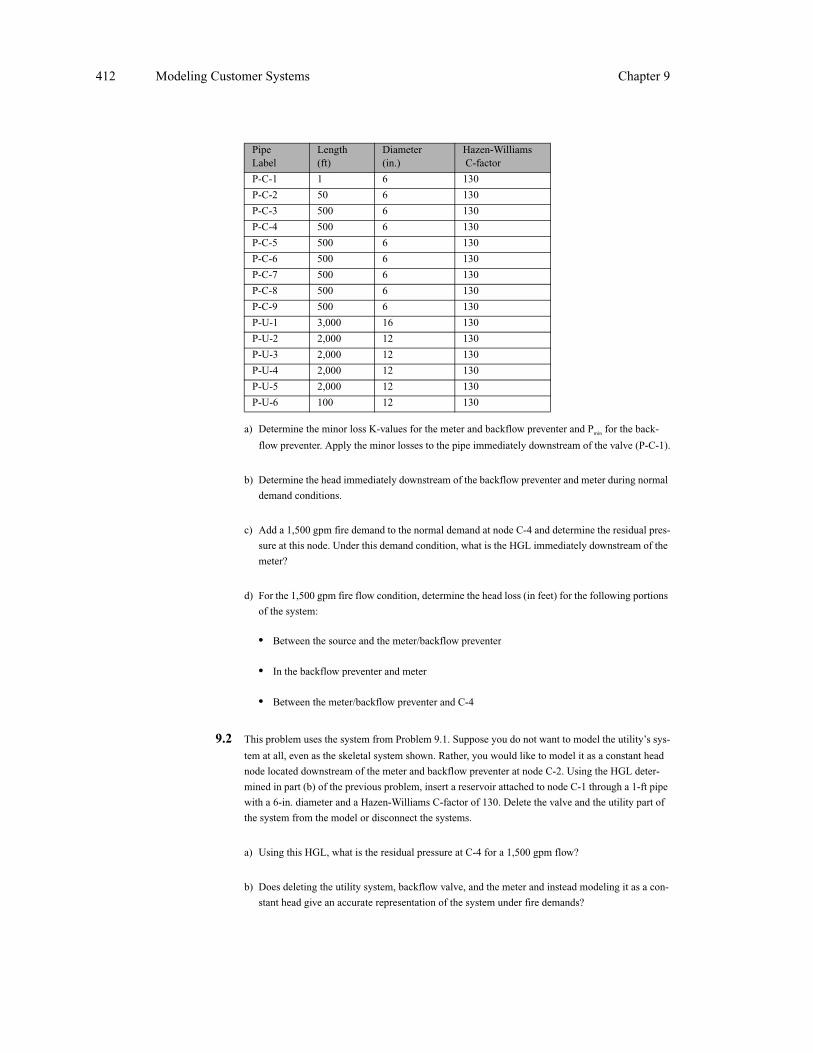
9.1 The water system for an industrial facility takes water from the utility’s system through a meter and reduced pressure backflow preventer. The following figures show the industrial system piping con-nected to the skeletonized utility system and the head loss curves for the meter and backflow preven-ter. The total head at the water source in the utility’s system is 320 ft, and the elevation of the backflow preventer is 90 ft. The meter and backflow preventer are located on pipe P-C-1, a nominal 6-in. pipe. Construct a model of the system under normal demand conditions using the data provided below.

U-4

Utility Res. U-2

U-1

C-3

PBV-1

C-2

C-7

C-5

C-4

C-6

C-1

U-3

(Not to scale)

Utility System

Industrial System

Meter and Backflow Valve

P-U-1 P-U-

2 P-U-3

P-U-

4P-U-5

P-U-6

P-C

-3

P-C-4

P-C

-5P-C

-6

P-C-7

P-C

-8

P-C-9

P-C-1P-C-2

Discussion Topics and Problems 411

NodeLabel

Elevation(ft)

Demand(gpm)

C-1 90.0 0

C-2 120.0 5

C-3 100.0 5

C-4 135.0 5

C-5 140.0 5

C-6 135.0 5

C-7 130.0 5

U-1 100.0 200

U-2 95.0 500

U-3 80.0 700

U-4 100.0 200

0

5

10

15

20

25

0 300 600 900 1200 1500

Flow, gpm

Pre

ssure

dro

p,psi

RPBP

Meter


a) Determine the minor loss K-values for the meter and backflow preventer and Pmin for the back-

flow preventer. Apply the minor losses to the pipe immediately downstream of the valve (P-C-1).

b) Determine the head immediately downstream of the backflow preventer and meter during normal

demand conditions.

c) Add a 1,500 gpm fire demand to the normal demand at node C-4 and determine the residual pres-

sure at this node. Under this demand condition, what is the HGL immediately downstream of the

meter?

d) For the 1,500 gpm fire flow condition, determine the head loss (in feet) for the following portions

of the system:

• Between the source and the meter/backflow preventer

• In the backflow preventer and meter

• Between the meter/backflow preventer and C-4

9.2 This problem uses the system from Problem 9.1. Suppose you do not want to model the utility’s sys-

tem at all, even as the skeletal system shown. Rather, you would like to model it as a constant head

node located downstream of the meter and backflow preventer at node C-2. Using the HGL deter-

mined in part (b) of the previous problem, insert a reservoir attached to node C-1 through a 1-ft pipe

with a 6-in. diameter and a Hazen-Williams C-factor of 130. Delete the valve and the utility part of

the system from the model or disconnect the systems.

a) Using this HGL, what is the residual pressure at C-4 for a 1,500 gpm flow?

b) Does deleting the utility system, backflow valve, and the meter and instead modeling it as a con-

stant head give an accurate representation of the system under fire demands?

PipeLabel

Length(ft)

Diameter(in.)

Hazen-Williams C-factor

P-C-1 1 6 130

P-C-2 50 6 130

P-C-3 500 6 130

P-C-4 500 6 130

P-C-5 500 6 130

P-C-6 500 6 130

P-C-7 500 6 130

P-C-8 500 6 130

P-C-9 500 6 130

P-U-1 3,000 16 130

P-U-2 2,000 12 130

P-U-3 2,000 12 130

P-U-4 2,000 12 130

P-U-5 2,000 12 130

P-U-6 100 12 130


9.3 An existing small irrigation system consists of five sprinklers in Area A, as shown in the figure below. A new landscaped area (Area B) of roughly the same size is planned, requiring that an addi-tional five sprinklers be installed.

Water for the existing irrigation system is pumped from a nearby pond. The owner would like to use the existing 1.5 hp pump to supply the additional sprinklers as well. Manufacturer pump curve data for this pump is provided in the following tables. The elevation of the pump is 97 ft.

Construct a steady-state hydraulic model of the sprinkler system if the pond water surface is at an elevation of 101 ft. Pipes M-3 and M-4 are both equipped with a 1-in. gate valve (K = 0.39) for isolating the system if necessary (for repairs and so forth) and a 1-in. anti-siphon valve (K = 14) to prevent contamination of the pond with substances such as chemical fertilizers.

To model the sprinklers, attach a reservoir with an HGL elevation equivalent to the sprinkler head elevation to the sprinkler node with an equivalent pipe.

According to the sprinkler manufacturer’s information, a pressure of 30 psi is required at the sprin-kler head to produce a discharge of 1.86 gpm. At this flow, the radius of the sprinkler coverage is 15 ft. The sprinkler spacing was determined based on this radius. Given this information, use Equation 9.4 to solve for the sprinkler coefficient, K, and determine the characteristics of the equivalent pipe as discussed in Section 9.5.

M-1

L-6

L-9

L-2

M-4

L-7

M-2

S-6

L-10

S-4

M-3 L-4

L-5

S-3S-2

S-9

J-2

J-3

S-7

S-1 L-3

L-8

L-1

S-8

J-1

Pond

Pump

S-10

S-5

LandscapeArea A

LandscapeArea B

PVC Main (typ.)

PVC Lateral (typ.)

Water Intake

Sprinkler (typ.)

Anti-

sipho

nva

lve(typ

.)

Gateva

lve(typ

.)


SprinklerLabel

Elevation(ft)

S-1 115.45

S-2 115.40

S-3 115.25

S-4 115.15

S-5 115.10

S-6 115.75

S-7 116.00

S-8 116.10

S-9 115.55

S-10 115.80

NodeLabel

Elevation(ft)

J-1 115

J-2 115

J-3 115

MainLabel

Length(ft)

Hazen-Williams C-factor

M-1 19 150

M-2 80 150

M-3 12 150

M-4 12 150

LateralLabel

Length(ft)

Hazen-WilliamsC-factor

L-1 17 150

L-2 26 150

L-3 26 150

L-4 16 150

L-5 26 150

L-6 16 150

L-7 26 150

L-8 26 150

L-9 17 150

L-10 26 150


a) The existing system uses ¾-in. laterals and 1-in. mains. Run the model with only the existing sys-tem in operation (that is, close pipe M-3). Is the pump able to adequately supply all of the sprin-klers? What is the minimum sprinkler discharge?

b) Re-run the model with all sprinklers (existing and proposed) open. Use ¾-in. laterals and 1-in. mains for both existing and proposed piping. Is the pump able to adequately supply all of the sprinklers? What is the minimum sprinkler discharge?

c) If you were designing the entire system from scratch (no pipes have been installed yet), what minimum size must the mains and laterals be to meet the minimum flow/pressure requirement? Assume all sprinklers are discharging simultaneously and the pump is the same as described in the preceding tables.

d) The owner obviously prefers to continue using the existing piping and would like to save on expenses by using smaller pipes in the new system as well. What could be done operationally to make such a design work?

9.4 This problem is a continuation of Problem 9.3. The irrigation system will be used to water the land-scaped areas for 2.5 hours each day. A schedule is established such that Area A will be watered from 4:00 a.m. to 6:30 a.m., and Area B from 6:30 a.m. to 9:00 a.m. The pipe sizes to be used are ¾-in. laterals and 1-in. mains.

a) Using the existing pump and given the minimum system requirements from Problem 9.3, can adequate flow/pressure be supplied at all of the sprinklers?

b) You are concerned about whether the pond has enough water for irrigation during a dry spell. Volume data for the pond is provided in the following tables. Model the pond as a tank using this volume data, and run an EPS to determine the total volume of water used by the irrigation system in a daily cycle. Neglecting evaporation and infiltration, extrapolate this rate of consumption to determine how long could a dry spell last before the pond runs dry.

Pump Curve Data

Head(ft)

Flow(gpm)

Shutoff 230 0

Design 187 10

Max Operating 83 20

Pond Data

Total Pond Volume 10,000 ft3

Maximum Pond Elevation 104 ft

Initial Pond Elevation 103 ft

Minimum Pond Elevation 98 ft

Pond Depth to Volume Ratios

DepthRatio

VolumeRatio

0.0 (elev. = 98 ft) 0.0 (vol. = 0)

0.5 (elev. = 101 ft) 0.3 (vol. = 3,000 ft3)

0.8 (elev = 102.8 ft) 0.7 (vol. = 7,000 ft3)

1.0 (elev. = 104 ft) 1.0 (vol. = 10,000 ft3)


9.5 For a building with an Ordinary Hazard Group 1 occupancy classification, the required minimum fire sprinkler capacity is 0.16 gpm/ft2 for a 1500 ft2 area. The coverage area for an individual sprin-kler is 130 ft2.

a) Compute the number of sprinklers required to provide coverage for a 1500 ft2 area.

b) What is the minimum discharge required from each sprinkler to meet the capacity requirement for the 1500 ft2 area?

c) If the type of sprinkler being used has a K-value of 4.0, what pressure must be supplied at the sprinkler head to deliver the required flow?

9.6 Use the fixture unit method to estimate the peak design flow for a commercial office complex with the following fixture totals:

The complex has lawn irrigation, but it does not operate during peak demand times. The fire service is through a separate line. Therefore, the fire and irrigation demands need not be included in the cal-culation.

Determine the total number of fixture units and the design flow. If you would like a velocity of5 ft/s in the service line during peak flow, roughly what size pipe would you use?

32 urinals (flush valve)

60 water closets (flush valve)

50 sinks

2shower rooms with eight shower heads total

16 drinking fountains

2 dishwashers (3/4-in.)

4 kitchen sinks (3/4-in.)

4 hose connections (3/4-in.)

Documents

ADVANCED WATER DISTRIBUTION MODELING AND MANAGEMENT 1 Water systems... · 2009-03-12 · ADVANCED WATER DISTRIBUTION MODELING AND MANAGEMENT Authors Thomas M. Walski Donald V. Chase