Advanced SynopticM. D. Eastin QG Analysis: Vertical Motion

Advanced Synoptic M. D. Eastin

QG Analysis: Vertical Motion


QG Analysis

QG Theory

• Basic Idea• Approximations and Validity• QG Equations / Reference

QG Analysis

• Basic Idea• Estimating Vertical Motion

• QG Omega Equation: Basic Form• QG Omega Equation: Relation to Jet Streaks• QG Omega Equation: Q-vector Form

• Estimating System Evolution• QG Height Tendency Equation

• Diabatic and Orographic Processes• Evolution of Low-level Cyclones• Evolution of Upper-level Troughs


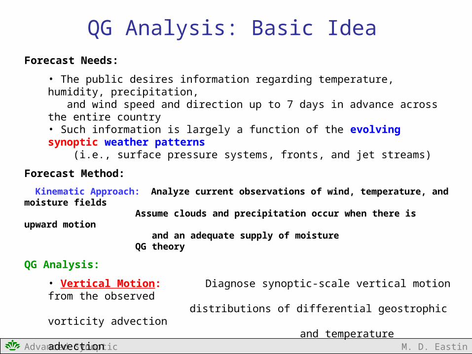
Forecast Needs:

• The public desires information regarding temperature, humidity, precipitation, and wind speed and direction up to 7 days in advance across the entire country• Such information is largely a function of the evolving synoptic weather patterns (i.e., surface pressure systems, fronts, and jet streams)

Forecast Method:

Kinematic Approach: Analyze current observations of wind, temperature, and moisture fields Assume clouds and precipitation occur when there is upward motion and an adequate supply of moisture QG theory

QG Analysis:

• Vertical Motion: Diagnose synoptic-scale vertical motion from the observeddistributions of differential geostrophic vorticity

advection and temperature advection

• System Evolution: Predict changes in the local geopotential height patterns fromthe observed distributions of geostrophic vorticity

advectionand differential temperature advection

QG Analysis: Basic Idea


Estimating vertical motion in the atmosphere:

Our Challenge:

• We do not observe vertical motion• Vertical motions influence clouds and precipitation• Actual vertical motions are often several orders of magnitude smaller than their collocated horizontal air motions [ w ~ 0.01 → 10 m/s ]

[ u,v ~ 10 → 100 m/s ]

• Synoptic-scale vertical motions must be estimated from widely-spaced observations (i.e., the rawinsonde network) every 12-hours

Methods:

• Kinematic Method Integrate the Continuity EquationVery sensitive to small errors in winds measurements

• Adiabatic Method From the thermodynamic equationVery sensitive to temperature tendencies

(difficult to observe)Difficult to incorporate impacts of diabatic

heating

QG Omega Equation Least sensitive to small observational errorsWidely believed to be the best method

QG Analysis: Basic Idea


Two Prognostic Equations – We Need Two Unknowns:

• In order to analyze vertical motion, we need to combine our two primary prognostic equations – for ζg and T – into a single equation for ω

• These 2 equations have 3 prognostic variables (ζg, T, and ω) → we want to keep ω•We need to convert both ζg and T into a common prognostic variable

Common Variable: Geopotential-Height Tendency (χ):

• We define a local change (or tendency) in geopotential-height:

wheret

QG Analysis: A Closed System of Equations

AdiabaticThermodynamic

Equation

VorticityEquationp

ffVt ggg

0)(

R

pTV

t

Tg

zg


Expressing Vorticity in terms of Geopotential Height:

• Begin with the definition of geostrophic relative vorticity:

where

• Substitute using the geostrophic wind relations, and one can easily show:

where

• We can now define local changes in geostrophic vorticity in terms of geopotential height and local height tendency (on pressure surfaces)

y

u

x

v ggg

yf

ug

0

1

xfvg

0

1

2

0

1

fg 2

2

2

22

yx

2

0

2

0

11

ffttg



Expressing Temperature in terms of Geopotential Height:

• Begin with the hydrostatic relation in isobaric coordinates:

• Using some algebra, one can easily show:

• We can now define local changes in temperature in terms of geopotential height and local height tendency (on pressure surfaces)

pR

pT

p

RT

p

pR

p

pR

p

tt

T



Note: These two equations will used to obtain the QG omega equation and, eventually, the QG height-tendency equation

Two Prognostic Equations – We Need Two Unknowns:

• We can now used these relationships to construct a closed system with two prognostic equations and two prognostic variables:

2

0

1

fg 2

0

2

0

11

ffttg

pR

pT

pR

p

pR

p

tt

T

pffV

t ggg

0)(p

fff

Vf o

go

022 11

R

pTV

t

Tg

R

p

pR

pV

pR

pg



The QG Omega Equation:

We can also derive a single diagnostic equation for ω by combining our modified vorticity and thermodynamic equations (the height-tendency versions):

To do this, we need to eliminate the height tendency (χ) from both equations

Step 1: Apply the operator to the vorticity equation

Step 2: Apply the operator to the thermodynamic equation

Step 3: Subtract the result of Step 1 from the result of Step 2

After a lot of math, we get the resulting diagnostic equation……


p

f

0

2pR

pff

fV

f og

o

022 11

R

p

pR

pV

pR

pg


The QG Omega Equation:

• This is (2.29) in the Lackmann text• This form of the equation is not very intuitive since we transformed geostrophic vorticity and temperature into terms of geopotential height.• To make this equation more intuitive, let’s transform them back…


TVp

RfV

p

f

p

fggg

202

2202

pR

pV

p

Rf

fV

p

f

p

fg

og

2202

2202 1

2

0

1

fg pR

pT


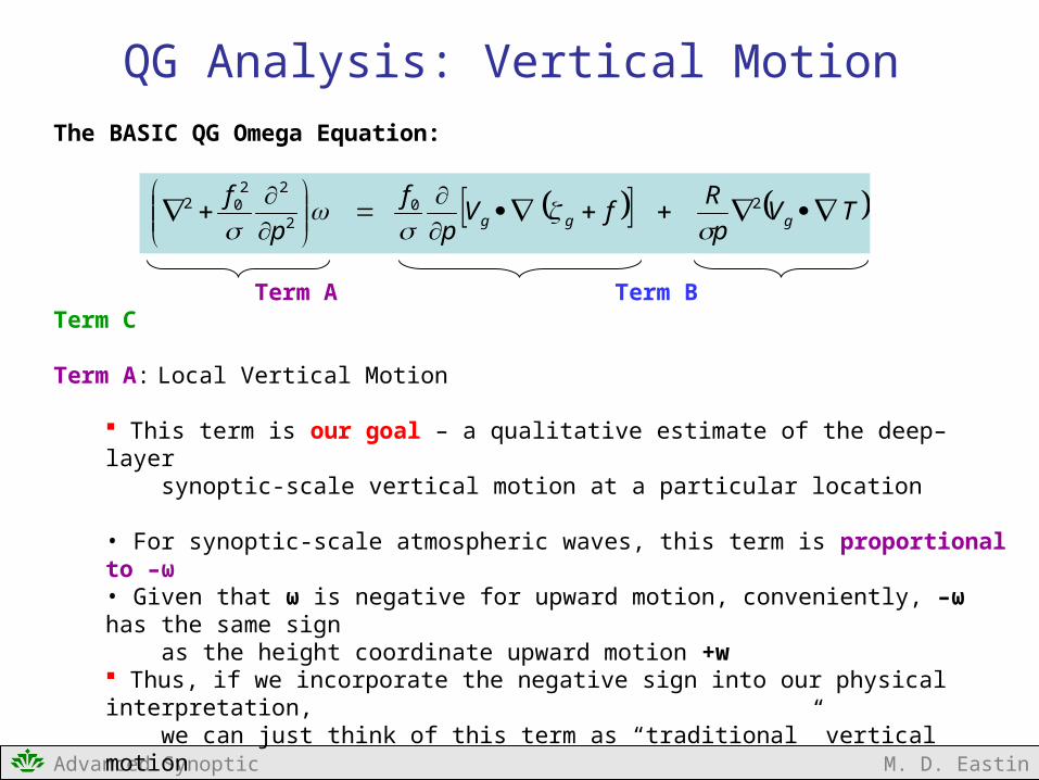
The BASIC QG Omega Equation:

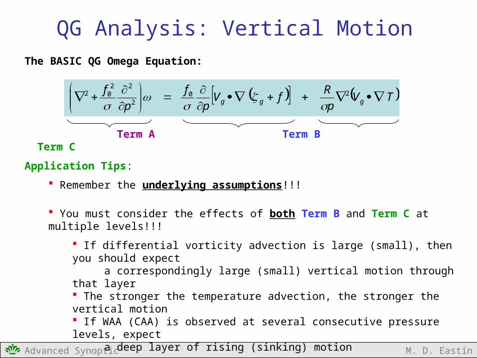
Term A Term B Term C

• To obtain an actual value for ω (the ideal goal), we would need to compute the forcing terms (Terms B and C) from the three-dimensional wind and temperature fields, and then invert the operator in Term A using a numerical procedure, called “successive over-relaxation”, with appropriate boundary conditions

• This is NOT a simple task (forecasters never do this)…..

Rather, we can infer the sign and relative magnitude of ω through simple inspection of the three-dimensional absolute geostrophic vorticity and temperature fields (forecasters do this all the time…)

Thus, let’s examine the physical interpretation of each term….

TVp

RfV

p

f

p

fggg

202

2202





Term A: Local Vertical Motion

This term is our goal – a qualitative estimate of the deep–layer synoptic-scale vertical motion at a particular location

• For synoptic-scale atmospheric waves, this term is proportional to –ω• Given that ω is negative for upward motion, conveniently, –ω has the same sign as the height coordinate upward motion +w Thus, if we incorporate the negative sign into our physical interpretation, we can just think of this term as “traditional” vertical motion


TVp

RfV

p

f

p

fggg

202

2202




Term B: Vertical Derivative of Absolute Geostrophic Vorticity Advection (Differential Vorticity Advection)

Single Pressure Level:

• Positive vorticity advection (PVA) PVA → causes local vorticity increases

• From our relationship between ζg and χ, we know that PVA is equivalent to:

therefore: PVA → or, since: PVA →

Thus, we know that PVA at a single level leads to height falls Using similar logic, NVA at a single level leads to height rises


0tg

2

0

1p

g

ft

02 p 0 2

TVp

RfV

p

f

p

fggg

202

2202





Multiple Pressure Levels

• Consider a three-layer atmosphere where PVA is strongest in the upper layer:

WAIT! Hydrostatic balance (via the hypsometric equation) requires ALL changes in thickness (ΔZ) to be accompanied by temperature changes.BUT these thickness changes were NOT a result of temperature changes…


TVp

RfV

p

f

p

fggg

202

2202

PVA

PVA

PVA

Z-top

Z-400mb

Z-700mb

Z-bottom

ΔZ decreasesΔZ PressureSurfaces

Fell ΔZ ΔZ decreases

UpperSurfacesFell More

ThicknessChanges





• In order to maintain hydrostatic balance, any thickness decreases must be accompanied by a temperature decrease or cooling• Recall our adiabatic assumption

• Therefore, in the absence of temperature advection and diabatic processes:

An increase in PVA with height will induce rising motion


TVp

RfV

p

f

p

fggg

202

2202

RisingMotions

AdiabaticCooling

SinkingMotions

AdiabaticWarming





Possible rising motion scenarios: Strong PVA in upper levelsWeak PVA in lower levels

PVA in upper levelsNo vorticity advection in lower levels

PVA in upper levels NVA in lower levels

Weak NVA in upper levelsStrong NVA in lower levels


TVp

RfV

p

f

p

fggg

202

2202





Multiple Pressure Levels

• Consider a three-layer atmosphere where NVA is strongest in the upper layer:

WAIT! Hydrostatic balance (via the hypsometric equation) requires ALL changes in thickness (ΔZ) to be accompanied by temperature changes.BUT these thickness changes were NOT a result of temperature changes…


TVp

RfV

p

f

p

fggg

202

2202

UpperSurfaces

Rose More

ThicknessChanges

NVA

NVA

NVA

Z-top

Z-400mb

Z-700mb

Z-bottom

ΔZ increasesΔZ

PressureSurfaces

Rose

ΔZ ΔZ increases





• In order to maintain hydrostatic balance, any thickness increases must be accompanied by a temperature increase or warming• Recall our adiabatic assumption

• Therefore, in the absence of temperature advection and diabatic processes:

An increase in NVA with height will induce sinking motion


TVp

RfV

p

f

p

fggg

202

2202

RisingMotions

AdiabaticCooling

SinkingMotions

AdiabaticWarming





Possible rising motion scenarios: Strong NVA in upper levelsWeak NVA in lower levels

NVA in upper levelsNo vorticity advection in lower levels

NVA in upper levels PVA in lower levels

Weak PVA in upper levelsStrong PVA in lower levels


TVp

RfV

p

f

p

fggg

202

2202





Strong NVA

Weaker NVA below(not shown)

Expect Sinking Motion

Strong PVA

Weaker PVA below(not shown)

Expect Rising Motion

Full-PhysicsModel

Analysis



Expected Rising Motion

ExpectedSinkingMotion



Generallyconsistent

with expectations!


QG Analysis: Vertical MotionThe BASIC QG Omega Equation:


Generally Consistent…BUT Noisy → Why?

• Only evaluated one level (500mb) → should evaluate multiple levels• Used full wind and vorticity fields → should use geostrophic wind and vorticity• Mesoscale-convective processes → QG focuses on only synoptic-scale (small Ro)• Condensation / Evaporation → neglected diabatic processes• Complex terrain → neglected orographic effects• Did not consider temperature (thermal) advection (Term C)!!!

• Yet, despite all these caveats, the analyzed vertical motion pattern is qualitatively consistent with expectations from the QG omega equation!!!




Term C: Geostrophic Temperature Advection (Thermal Advection)

• Warm air advection (WAA) leads to local temperature / thickness increases• Consider the three-layer model, with WAA strongest in the middle layer

WAIT! Local geopotential height rises (falls) produce changes in the local height gradients → changing the local geostrophic wind and vorticity

BUT these thickness changes were NOT a result of geostrophic vorticity changes…


WAA

Z-400mb

Z-700mb

Z-bottom

ΔZ increasesΔZ

SurfaceRose

Z-top

SurfaceFell

TVp

RfV

p

f

p

fggg

202

2202





• In order to maintain geostrophic flow, any thickness changes must be accompanied by ageostrophic divergence (convergence) in regions of height rises (falls), which via mass continuity requires a vertical motion through the layer

• Therefore, in the absence of geostrophic vorticity advection and diabatic processes:

WAA will induce rising motion


Z-400mb

Z-700mb

Z-bottom

ΔZ increase

SurfaceRose

Z-top

SurfaceFell

Z-400mb

Z-700mb

Z-bottom

Z-top

TVp

RfV

p

f

p

fggg

202

2202

py

v

x

u agag

QG Mass Continuity





• Cold air advection (CAA) leads to local temperature / thickness decreases• Consider the three-layer model, with CAA strongest in the middle layer

WAIT! Local geopotential height rises (falls) produce changes in the local height gradients → changing the local geostrophic wind and vorticity

BUT these thickness changes were NOT a result of geostrophic vorticity changes…


TVp

RfV

p

f

p

fggg

202

2202

CAAZ-400mb

Z-700mb

Z-bottom

ΔZ

SurfaceRose

Z-topSurface

Fell

ΔZ decreases





• In order to maintain geostrophic flow, any thickness changes must be accompanied by ageostrophic divergence (convergence) in regions of height rises (falls), which via mass continuity requires a vertical motion through the layer

• Therefore, in the absence of geostrophic vorticity advection and diabatic processes:

CAA will induce sinking motion


TVp

RfV

p

f

p

fggg

202

2202

py

v

x

u agag

QG Mass Continuity

Z-400mb

Z-700mb

Z-bottom

ΔZ decreaseSurfaceRose

Z-topSurface

Fell Z-400mb

Z-700mb

Z-bottom

Z-top





Strong CAA

Expect Sinking Motion

Strong WAA

Expect Rising Motion

Full-PhysicsModel

Analysis





Strong CAA

Expected Sinking Motion

Strong WAA

Expected Rising Motion

Somewhatconsistent

with expectations…


QG Analysis: Vertical MotionThe BASIC QG Omega Equation:


Somewhat Consistent…BUT very noisy → Why?

• Used full wind field → should use geostrophic wind• Only evaluated one level (850mb) → should evaluate multiple levels• Mesoscale-convective processes → QG focuses on only synoptic-scale (small Ro)• Condensation / Evaporation→ neglected diabatic processes• Complex terrain → neglected orographic effects• Did not consider differential vorticity advection (Term B)!!!

• Yet, despite all these caveats, the analyzed vertical motion pattern is still somewhat consistent with expectations from the QG omega equation!!!




Application Tips:

Remember the underlying assumptions!!!

You must consider the effects of both Term B and Term C at multiple levels!!!

If differential vorticity advection is large (small), then you should expect a correspondingly large (small) vertical motion through that layer The stronger the temperature advection, the stronger the vertical motion If WAA (CAA) is observed at several consecutive pressure levels, expect a deep layer of rising (sinking) motion

Opposing expectations from the two terms at a given location will weaken the total vertical motion (and complicate the interpretation)!!! [more on this later]


TVp

RfV

p

f

p

fggg

202

2202




Application Tips:

The QG omega equation is a diagnostic equation:

• The equation does not predict future vertical motion patterns The forcing functions (Terms B and C) produce instantaneous responses

• Use of the QG omega equation in a diagnostic setting:

• Diagnose the synoptic–scale vertical motion pattern, and assume rising motion corresponds to clouds and precipitation when ample moisture is available Compare to the observed patterns → can infer mesoscale contributions Helps distinguish between areas of persistent light precipitation (synoptic-scale) and more sporadic intense precipitation (mesoscale)


TVp

RfV

p

f

p

fggg

202

2202


Review of Jet Streaks:

• Air parcels accelerate just upstream into the “entrance” region and then decelerate downstream coming out of the “exit” region (for an observer facing downstream)

• Often sub-divided into quadrants:

• Right Entrance (or R-En)• Left Entrance (or L-En)• Right Exit (or R-Ex)• Left Exit (or L-Ex)

• Each quadrant has an “expected” vertical motion….WHY?

Jet Streak

LeftExit

RightExit

LeftEntrance

RightEntrance

Descent

Ascent

Ascent

Descent

QG Analysis: Application to Jet Streaks


QG Analysis: Application to Jet StreaksPhysical Interpretation:


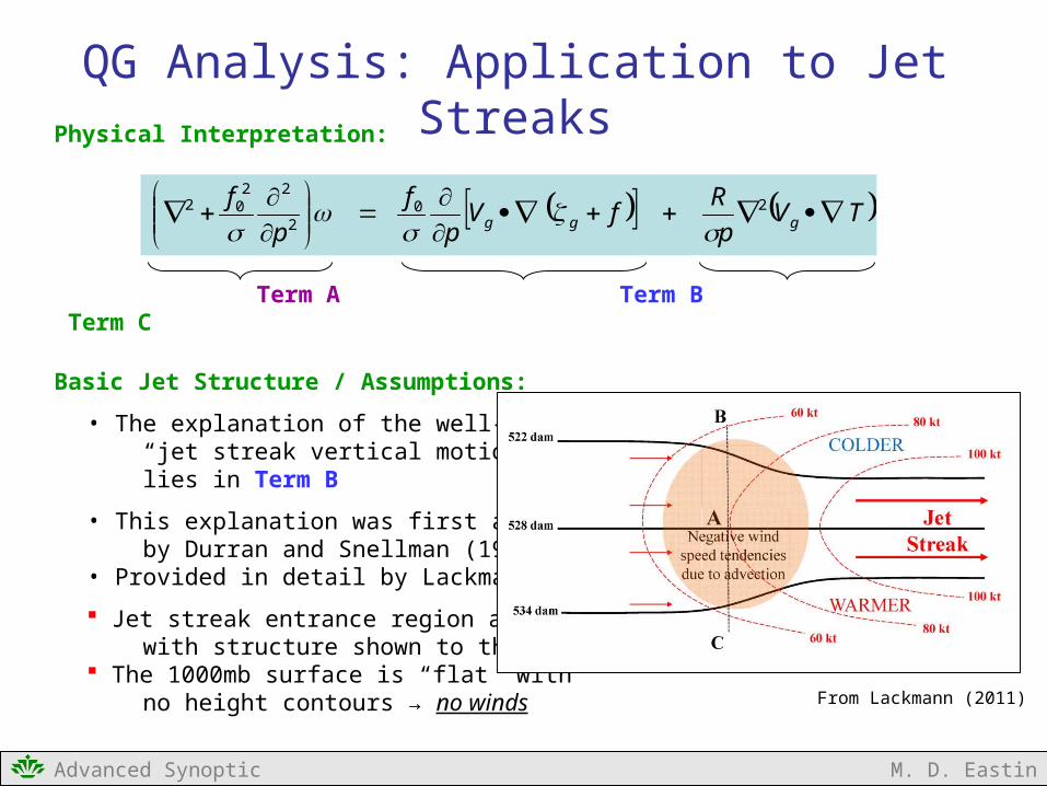
Basic Jet Structure / Assumptions:

• The explanation of the well-known “jet streak vertical motion pattern” lies in Term B

• This explanation was first advanced by Durran and Snellman (1987)• Provided in detail by Lackmann text

Jet streak entrance region at 500mb with structure shown to the right The 1000mb surface is “flat” with no height contours → no winds

TVp

RfV

p

f

p

fggg

202

2202

From Lackmann (2011)




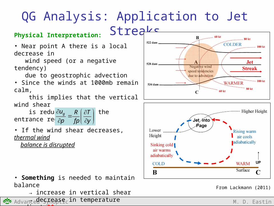
Physical Interpretation:

• Near point A there is a local decrease in wind speed (or a negative tendency) due to geostrophic advection• Since the winds at 1000mb remain calm, this implies that the vertical wind shear is reduced through the entrance region

• If the wind shear decreases, thermal wind balance is disrupted

• Something is needed to maintain balance → increase in vertical shear → decrease in temperature gradient **

Since geostrophic flow disrupted balance (!) ageostrophic flow must bring about the return to balance by weakening the thermal gradient via adiabatic vertical motions and mass continuity!

y

T

fp

R

p

ug





• With respect to differential vorticity advection (Term B), at 500mb, cyclonic vorticity (+) is located north of the jet streak, with anti- cyclonic vorticity (–) located to the south

Left Entrance region → AVA (or NVA) Right Entrance region → CVA (or PVA)

• With no winds at 1000mb → no vorticity advection

• Thus, evaluation of Term B implies:

L-En → Term B < 0 → Sinking Motion R-En → Term B > 0 → Rising Motion

L-En

R-En

R-EnL-En


QG Analysis: Application to Jet StreaksPhysical Interpretation:

• Thus, the “typical” vertical motion pattern associated with jet streaks arises from QG forcing associated with differential vorticity advection!

Important Points:

The atmosphere is constantly advecting itself out of thermal wind balance. Even advection by the geostrophic flow can destroy balance.

Ageostrophic secondary circulations, with vertical air motions, arise as a response and return the atmosphere to balance

Descent

DescentAscent

Ascent


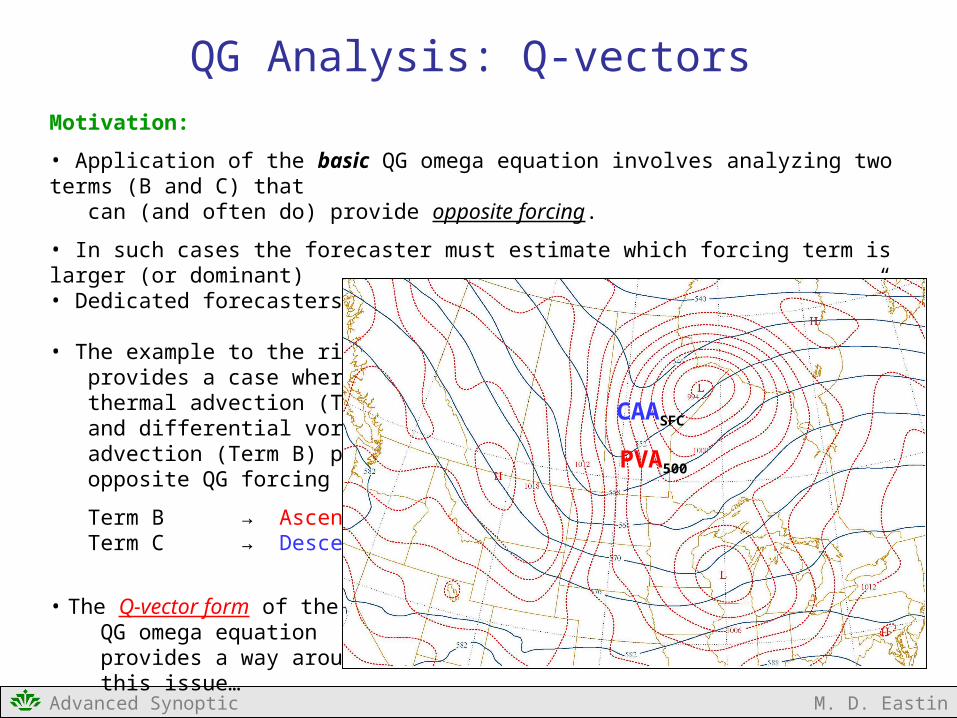
QG Analysis: Q-vectorsMotivation:

• Application of the basic QG omega equation involves analyzing two terms (B and C) that can (and often do) provide opposite forcing.

• In such cases the forecaster must estimate which forcing term is larger (or dominant)• Dedicated forecasters find such situations and “unsatisfactory”

• The example to the right provides a case where thermal advection (Term C) and differential vorticity advection (Term B) provide opposite QG forcing

Term B → Ascent Term C → Descent

• The Q-vector form of the QG omega equation provides a way around this issue…

CAASFC

PVA500


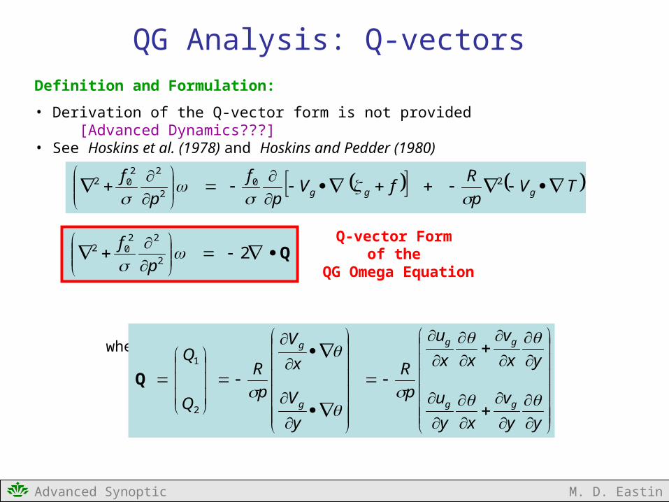
QG Analysis: Q-vectorsDefinition and Formulation:

• Derivation of the Q-vector form is not provided [Advanced Dynamics???]• See Hoskins et al. (1978) and Hoskins and Pedder (1980)

where:

TVp

RfV

p

f

p

fggg

202

2202

Q

22

2202 p

f Q-vector Formof the

QG Omega Equation

yy

v

xy

u

yx

v

xx

u

p

R

y

V

x

V

p

R

Q

Q

gg

gg

g

g

2

1

Q



where

• The components Q1 and Q2 provide a measure of the horizontal wind shear across a temperature gradient in the zonal and meridional directions• The two components can be combined to produce a horizontal “Q-vector”

Q-vectors are oriented parallel to the ageostrophic wind vector Q-vectors are proportional to the magnitude of the ageostrophic wind Q-vectors point toward rising motion

In regions where:

Q-vectors converge → Ascent

Q-vectors diverge → Descent

QG Analysis: Q-vectors

Q

22

2202 p

f

yy

v

xy

u

yx

v

xx

u

p

R

Q

Q

gg

gg

2

1

Q


QG Analysis: Q-vectorsPhysical Interpretation: Hypothetical Case

• Synoptic-scale low pressure system (center at C)• Meridional flow shown by black vectors (no zonal flow)• Warm air to the south and cold air to the north (no zonal thermal gradient)

• Regions of Q-vector forcing for vertical motion are exactly consistent with what one would expect from the basic form of the QG omega equation

WAA → Ascent CAA → Descent

Q1 Q1Q1

WAA

CAA


Example:

850-mb Analysis – 29 July 1997 at 00ZIsentropes (red), Q-vectors, Vertical motion (shading, upward only)



Example:


500-mb GFS Forecast – 13 September 2008 at 1800Z500-mb Heights (black), Q-vectors, Q-vector convergence (blue) and divergence (red)


Application Tips:

where

Advantages:

• Only one forcing term → no partial cancellation of opposite forcing terms • All forcing can be evaluated on a single isobaric surface → should use multiple levels

• Can be easily computed from 3-D data fields (quantitative)• The Q-vectors computed from numerical model output can be plotted on maps to obtain a clear representation of synoptic-scale vertical motion

Disadvantages:

• Can be very difficult to estimate from standard upper-air observations• Neglects diabatic heating• Neglects orographic effects


Q

22

2202 p

f

yy

v

xy

u

yx

v

xx

u

p

R

Q

Q

gg

gg

2

1

Q


ReferencesBluestein, H. B, 1993: Synoptic-Dynamic Meteorology in Midlatitudes. Volume I: Principles of Kinematics and Dynamics.

Oxford University Press, New York, 431 pp.

Bluestein, H. B, 1993: Synoptic-Dynamic Meteorology in Midlatitudes. Volume II: Observations and Theory of WeatherSystems. Oxford University Press, New York, 594 pp.

Charney, J. G., B. Gilchrist, and F. G. Shuman, 1956: The prediction of general quasi-geostrophic motions. J. Meteor.,13, 489-499.

Durran, D. R., and L. W. Snellman, 1987: The diagnosis of synoptic-scale vertical motionin an operational environment. Weather and Forecasting, 2, 17-31.

Hoskins, B. J., I. Draghici, and H. C. Davis, 1978: A new look at the ω–equation. Quart. J. Roy. Meteor. Soc., 104, 31-38.

Hoskins, B. J., and M. A. Pedder, 1980: The diagnosis of middle latitude synoptic development. Quart. J. Roy. Meteor.Soc., 104, 31-38.

Lackmann, G., 2011: Mid-latitude Synoptic Meteorology – Dynamics, Analysis and Forecasting, AMS, 343 pp.

Trenberth, K. E., 1978: On the interpretation of the diagnostic quasi-geostrophic omega equation. Mon. Wea. Rev., 106,131-137.

Documents

Advanced SynopticM. D. Eastin QG Analysis: Vertical Motion