Embed Size (px)
Citation preview

Advanced Street Lighting Technologies Assessment Project - City of San Jose
100% FINAL, August 13, 2010
Revision 1.0 December 10, 2010
Prepared by:
Michael Mutmansky, Todd Givler, Jessica Garcia, and Nancy Clanton
Clanton & Associates, Inc.
With sections by:
Dr. Ronald Gibbons and Christopher Edwards
Virginia Tech Transportation Institute
Sponsored by:
City of San Jose, California
Street Lighting Assessment Project – City of San Jose
Clanton & Associates, Inc. Page ii
December 10, 2010
Project Team
This project is funded by the City of San Jose with Laura Stuchinsky as project manager. Michael Mutmansky of Clanton & Associates, Inc. of Boulder, Colorado developed and executed the survey portion of the project with the support of Todd Givler, Jessica Garcia, and Nancy Clanton. The lead author of this report is Jessica Garcia. Dr. Ron Gibbons and Chris Edwards of the Virginia Tech Transportation Institute developed, performed, and reported the visibility ‘performance’ tests described in this report.
Disclaimer
This report was prepared as an account of work funded by the City of San Jose. While this document is believed to contain correct information, neither Clanton & Associates, Inc., Virginia Tech Transportation Institute, the City of San Jose, nor any employees or associates, makes any warranty, expressed or implied, or assumes any legal responsibility for the accuracy, completeness, or usefulness of any information, apparatus, product, or process disclosed, or represents that its use would not infringe privately owned rights. References herein to any specific commercial product, process or service by its trade name, trademark, manufacturer, or otherwise, does not necessarily constitute or imply its endorsement, recommendation, or favoring by Clanton & Associates, Inc., Virginia Tech Transportation Institute, nor the City of San Jose, their employees, associates, officers, or members. The ideas, views, opinions, and findings of authors expressed herein do not necessarily state or reflect those of the City of San Jose. Such ideas, views, opinions or findings should not be construed as an endorsement to the exclusion of others that may be suitable. The contents, in whole or part, shall not be used for advertising or product endorsement purposes. Any reference to an external hyperlink does not constitute an endorsement. Although efforts have been made to provide complete and accurate information, the information should always be verified before it is used in any way.
Acknowledgements
This demonstration was completed with the equipment contributions made by the lighting manufacturers. We would like to acknowledge and thank the various vendors. Without their contributions, this assessment project would not have been possible.
Street Lighting Assessment Project – City of San Jose
Clanton & Associates, Inc. Page iii
December 10, 2010
Table of Contents
1.0 Introduction....................................................................................... 5
1.1 History and Background ........................................................................ 5
1.2 Technology and Market Overview ........................................................... 6
1.3 Prior Work........................................................................................... 6
2.0 Project Methodology .......................................................................... 8
2.1 Overall Project Setup ............................................................................ 8
2.2 Light Sources and Luminaires................................................................. 9
2.3 Multiple Light Levels ........................................................................... 11
2.3.1 Output.............................................................................................. 11
2.3.2 Power............................................................................................... 12
2.4 Lighting Calculations........................................................................... 12
2.5 Survey Approach................................................................................ 15
2.6 Subjective Survey .............................................................................. 16
2.7 Objective ‘Performance’ Visibility Test ................................................... 16
2.8 Experimental Design........................................................................... 17
2.9 Methods for Objective Testing .............................................................. 17
2.9.1 Participants ....................................................................................... 17
2.9.2 Equipment ........................................................................................ 17
2.9.3 Equipment - Roadway Lighting Mobile Measurement System (RLMMS) ....... 17
2.9.4 Equipment - Visibility Targets............................................................... 19
2.9.5 Contrast ........................................................................................... 21
2.10 Survey Night Site Conditions................................................................ 22
2.11 Photos .............................................................................................. 22
2.12 Procedure ......................................................................................... 24
2.13 Data Analysis..................................................................................... 25
3.0 Results ............................................................................................. 26
3.1 Electrical Demand and Energy Savings .................................................. 26
3.2 Calculated Lighting Values ................................................................... 28
3.2.1 Illuminance Calculations...................................................................... 28
3.2.2 Spectral Power Distribution Calculations ................................................ 29
3.3 Subjective Survey .............................................................................. 33
3.4 Objective Visibility Detection Distance ................................................... 34
3.4.1 Weather Impacts on Detection Distance ................................................ 39
3.5 Objective Visibility Illuminance ............................................................. 42
4.0 Discussion........................................................................................ 47
4.1 Energy Implications ............................................................................ 47
4.2 Street Lighting Dimming Controls ......................................................... 51
4.3 Subjective Survey Analysis .................................................................. 51
4.4 Objective Visibility Analysis.................................................................. 52
4.5 Light Color ........................................................................................ 53

Street Lighting Assessment Project – City of San Jose
Clanton & Associates, Inc. Page iv
December 10, 2010
4.6 Night Sky Considerations..................................................................... 54
4.7 Equivalent Driving Visibility.................................................................. 61
4.8 Adaptive Standards Opportunities......................................................... 62
4.9 Limitations of the Project..................................................................... 62
5.0 Conclusions ...................................................................................... 63
6.0 Appendix A: Subjective Lighting Survey Form.................................. 65
7.0 Appendix B: Subjective Survey Participant Comments ..................... 67
8.0 Appendix C: Luminaire Cutsheets..................................................... 74
9.0 Appendix D: Relative Sky Glow Spectral Calculations....................... 82
10.0 Appendix E: Site Calculations ........................................................... 97
11.0 Appendix F: Subjective Survey Results........................................... 104
12.0 Appendix G: Control Systems ......................................................... 115
13.0 Appendix H: Luminance Adjustment Factors .................................. 117
14.0 References ..................................................................................... 122

Street Lighting Assessment Project – City of San Jose
Clanton & Associates, Inc. Page v
December 10, 2010
Abbreviations and Acronyms
ASC Adaptive Street Lighting Control
ANCOVA ANalysis Of COVariance
AASHTO American Association of State Highway Authority and Transportation Officials
CAN Controller Area Network
CCT Correlated Color Temperature in degrees Kelvin
CIE International Commission on Illumination
CRI Color Rendering Index
DOE Department of Energy
FC Footcandles
FPS Frames per Second
GHG Greenhouse Gases
GPS Global Positioning Device
HPS High Pressure Sodium
IESNA Illuminating Engineering Society of North America
IND Induction
kWh Kilowatt Hour
LED Light Emitting Diode
LPS Low Pressure Sodium
LTI Lighting & Infrastructure Technology Group
MH Metal Halide
RLMMS Roadway Lighting Mobile Measurement System
SAS Statistical Analysis Software
SNK Student Neumann Keuls
SPD Spectral Power Distribution
STV Small Target Visibility
VTTI Virginia Tech Transportation Institute
W Watts

Street Lighting Assessment Project – City of San Jose
Clanton & Associates, Inc. Page vi
December 10, 2010
Definitions
Adaptation The process by which the visual system becomes accustomed to more or less light or of a different color than it was exposed to during an immediately preceding period. It results in a change in the sensitivity of the eye to light. (RP-8-05)
CIE 115 Lighting of Roads for Motor and Pedestrian Traffic
CIE 191 Recommended System for Mesopic Photometry Based on Visual Performance.
Cones Retinal receptors that dominate the retinal response when the luminance level is high and provide the basis for the perception of color. (RP-33-99)
Contrast Threshold The minimal perceptible contrast for a given state of adaptation of the eye. It also is defined as the luminance contrast detectable during some specific fraction of the times it is presented to an observer, usually 50 percent. (RP-8-05)
Luminous Efficacy of a light source
The total luminous flux emitted by a lamp divided by the total lamp power input. It is expressed in lumens per watt. (RP-33-99)
Footcandle The unit of illuminance when the foot is taken as the unit of length. It is the illuminance on a surface one square foot in area on which there is a uniformly distributed flux of one lumen, or the illuminance produced on a surface all points of which are at a distance of one foot from a directionally uniform point source of one candela. (RP-8-05)
Illuminance The density of the luminous flux incident on a surface; it is the quotient of the luminous flux by the area of the surface when the latter is uniformly illuminated. (RP-8-05)
Lumen The SI unit of luminous flux. (RP-33-99)
Luminance The quotient of the luminous flux at an element of the surface surrounding the point, and propagated in directions defined by an elementary cone containing the given direction, by the product of the solid angle of the cone and area of the orthogonal projection of the element of the surface on a plane perpendicular to the given direction. The luminous flux may be leaving, passing through, and/or arriving at the surface. Note: in common usage the term ‘brightness’ usually refers to the strength of sensation which results from viewing surfaces or spaces from which light comes to the eye. This sensation is determined in part by the definitely measurable luminance defined above and in part by conditions of observation such as the state of adaptation of the eye. (RP-8-05)
Luminance Contrast The relationship between the luminances of an object and its immediate background. (RP-8-05)
Luminous Flux Radiant flux (radiant power); the time rate of flow of radiant energy. (RP-33-99)
Street Lighting Assessment Project – City of San Jose
Clanton & Associates, Inc. Page vii
December 10, 2010
Lux The SI unit of illuminance. It is the illuminance on a surface one square meter in area on which there is a uniformly distributed flux of one lumen, or the illuminance produced at a surface all points of which are at a distance of one meter from a uniform point source of one candela. (RP-8-05)
Mesopic Vision Vision with fully adapted eyes at luminance conditions between those of photopic and scotopic vision, that is, between about 3 and 0.001 cd/m2 (0.3 and 0.0001 cd/ft2). (RP-33-99)
Photopic Vision Vision mediated essentially or exclusively by the cones. It is generally associated with adaptation to a luminance of at least 3 cd/m2 (0.3 cd/ft2). (RP-33-99)
Roadway Lighting Provided for freeways, expressways, limited access roadways, and roads on which pedestrians, cyclists, and parked vehicles are generally not present. The primary purpose of roadway lighting is to help the motorist remain on the roadway and help with the detection of obstacles within and beyond the range of the vehicles headlights.
Rods Retinal receptors which respond at low levels of luminance, even below the threshold for cones. At these levels there is no basis for perceiving differences in hue and saturation. No rods are found near the center of the fovea. (RP-33-99)
Scotopic Vision Vision mediated essentially or exclusively by the rods. It is generally associated with adaptation to luminance below about 0.001 cd/m2 (0.0001 cd/ft2). (RP-33-99)
Small Target Visibility (STV)
The STV method of design determines the visibility level of an array of targets on the roadway considering the following factors: the luminance of the targets; the luminance of the immediate background; the adaptation level of the adjacent surroundings; and disability glare. The weighted average of the visibility level of these targets results in the STV. (RP-8-05)
Street Lighting Provided for major, collector, and local roads where pedestrians and cyclists are generally present. The primary purpose of street lighting is to help the motorist identify obstacles, provide adequate visibility of pedestrians and cyclists, and assist in visual search tasks, both on and adjacent to the roadway.
System Wattage The total wattage of the lamp source and the ballast combined.
Visibility The quality or state of being perceivable by the eye. In many outdoor applications, visibility is sometimes defined in terms of the distance at which an object can be just perceived by the eye. In indoor and outdoor applications, it usually is defined in terms of the contrast or size of a standard test object, observed under standardized view-conditions, having the same threshold as the given object. (RP-8-05)
Street Lighting Assessment Project – City of San Jose
Clanton & Associates, Inc. Page viii
December 10, 2010
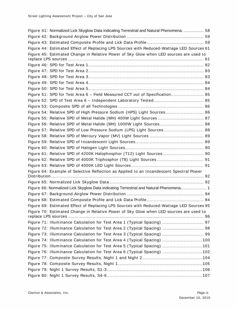
List of Figures
Figure 1: Scotopic, Mesopic and Photopic Ranges ......................................................... 6
Figure 2: Experiment Location and Set-Up for Entire Test Area. ...................................... 9
Figure 3: False-Color Rendering for Test Area 2 – Typical Spacing of 160’ ...................... 13
Figure 4: False-Color Rendering for Test Area 5 – Typical Spacing of 160’ ...................... 13
Figure 5: Plan View of Luminaire Distribution and Highlighted Roadway Surface.............. 14
Figure 6: Isometric View of Luminaire Uplight Distribution ........................................... 14
Figure 7: Experimental Vehicle with RLMMS Components. ........................................... 18
Figure 8: RLMMS Components mounted on and inside a vehicle ................................... 19
Figure 9: Detection Targets used within Test Areas ..................................................... 20
Figure 10: Experiment Location and Set-Up for Test Areas 1 and 2 ............................... 20
Figure 11: Experiment Location and Set-Up for Test Areas 3 and 4 ............................... 21
Figure 12: Experiment Location and Set-Up for Test Area 5 and 6................................. 21
Figure 13: Weber Contrast Equation ........................................................................ 21
Figure 14: Positive (left) and Negative (right) Contrast............................................... 22
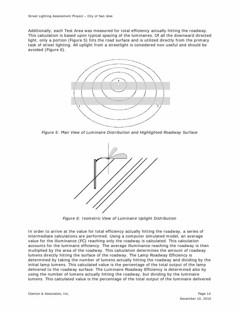
Figure 15: Photo of Survey Participant Briefing at the MLKJ Library. ............................. 23
Figure 16: Nighttime Photo of Survey Group under LPS Lighting. .................................. 23
Figure 17: Nighttime Photo of Survey Group under White Lighting. ............................... 24
Figure 18: SPD of Test Area 1 (IND) Measured CCT 3129K........................................... 30
Figure 19: SPD of Test Area 2 (HPS) Measured CCT 1894K .......................................... 30
Figure 20: SPD of Test Area 3 (LEDa) Measured CCT 5191K ......................................... 31
Figure 21: SPD of Test Area 4 (LPS) Measured CCT 1742K........................................... 31
Figure 22: SPD of Test Area 5 (LEDb) Measured CCT 3502K ......................................... 32
Figure 23: SPD of Test Area 6 (LEDc) Independently Tested Luminaire Results – Not Field Measured Data ...................................................................................................... 32
Figure 24: Subjective Survey Results for All Statements .............................................. 34
Figure 25: Test Area and Detection Distance Comparisons. .......................................... 36
Figure 26: Weber Contrast Calculations for Full and Low Settings by Target Color ........... 37
Figure 27: Test Area and Target Color (Full Output Test) ............................................. 38
Figure 28: Photopic and Mesopic Gray Target Detection Distance Comparisons ............... 39
Figure 29: Relative Detection Distance Night 1 – Full Setting........................................ 40
Figure 30: Relative Detection Distance Night 2 – Low Setting ....................................... 41
Figure 31: Relative Detection Distance and Watts per Linear Foot ................................. 42
Figure 32: Mean Illuminance Levels per Test Area and Survey Night.............................. 43
Figure 33: Mean Glare Meter Illuminance Levels ......................................................... 45
Figure 34: Typical Daylight Hours in San Jose, CA ........................................................ 1
Figure 35: Winter Street Lighting Use Profile.............................................................. 49
Figure 36: Spring/Fall Street Lighting Use Profile ........................................................ 49
Figure 37: Summer Street Lighting Use Profile ........................................................... 50
Figure 38: Detection Distance and Illuminance Levels by Test Area ............................... 53
Figure 39: Spectral Power Distribution Curves Comparing LPS, HPS and IND. ................. 55
Figure 40: Spectral Power Distribution Curves Comparing LPS and LED Sources.............. 56
Street Lighting Assessment Project – City of San Jose
Clanton & Associates, Inc. Page ix
December 10, 2010
Figure 41: Normalized Lick Skyglow Data indicating Terrestrial and Natural Phenomena. .............. 58
Figure 42: Background Airglow Power Distribution ...................................................... 59
Figure 43: Estimated Composite Profile and Lick Data Profile........................................ 59
Figure 44: Estimated Effect of Replacing LPS Sources with Reduced-Wattage LED Sources 61
Figure 45: Estimated Change in Relative Power of Sky Glow when LED sources are used to replace LPS sources ............................................................................................... 61
Figure 46: SPD for Test Area 1................................................................................. 82
Figure 47: SPD for Test Area 2................................................................................. 83
Figure 48: SPD for Test Area 3................................................................................. 83
Figure 49: SPD for Test Area 4................................................................................. 84
Figure 50: SPD for Test Area 5................................................................................. 84
Figure 51: SPD for Test Area 6 – Field Measured CCT out of Specification....................... 85
Figure 52: SPD of Test Area 6 – Independent Laboratory Tested................................... 85
Figure 53: Composite SPD of all Technologies ............................................................ 86
Figure 54: Relative SPD of High Pressure Sodium (HPS) Light Sources........................... 86
Figure 55: Relative SPD of Metal Halide (MH) 400W Light Sources ................................ 87
Figure 56: Relative SPD of Metal Halide (MH) 1000W Light Sources............................... 88
Figure 57: Relative SPD of Low Pressure Sodium (LPS) Light Sources ............................ 88
Figure 58: Relative SPD of Mercury Vapor (MV) Light Sources ...................................... 89
Figure 59: Relative SPD of Incandescent Light Sources................................................ 89
Figure 60: Relative SPD of Halogen Light Sources....................................................... 90
Figure 61: Relative SPD of 4200K Halophosphor (T12) Light Sources............................. 90
Figure 62: Relative SPD of 4000K Triphosphor (T8) Light Sources ................................. 91
Figure 63: Relative SPD of 4000K LED Light Sources................................................... 91
Figure 64: Example of Selective Reflection as Applied to an Incandescent Spectral Power Distribution ........................................................................................................... 92
Figure 65: Normalized Lick Skyglow Data .................................................................. 92 Figure 66: Normalized Lick Skyglow Data indicating Terrestrial and Natural Phenomena.................. 1
Figure 67: Background Airglow Power Distribution ...................................................... 94
Figure 68: Estimated Composite Profile and Lick Data Profile........................................ 94
Figure 69: Estimated Effect of Replacing LPS Sources with Reduced-Wattage LED Sources 95
Figure 70: Estimated Change in Relative Power of Sky Glow when LED sources are used to replace LPS sources ............................................................................................... 96
Figure 71: Illuminance Calculation for Test Area 1 (Typical Spacing) ............................. 97
Figure 72: Illuminance Calculation for Test Area 2 (Typical Spacing) ............................. 98
Figure 73: Illuminance Calculation for Test Area 3 (Typical Spacing) ............................. 99
Figure 74: Illuminance Calculation for Test Area 4 (Typical Spacing) ............................100
Figure 75: Illuminance Calculation for Test Area 5 (Typical Spacing) ............................101
Figure 76: Illuminance Calculation for Test Area 6 (Typical Spacing) ............................102
Figure 77: Composite Survey Results, Night 1 and Night 2..........................................104
Figure 78: Composite Survey Results, Night 1...........................................................105
Figure 79: Night 1 Survey Results, S1-3...................................................................106
Figure 80: Night 1 Survey Results, S4-6...................................................................107

Street Lighting Assessment Project – City of San Jose
Clanton & Associates, Inc. Page x
December 10, 2010
Figure 81: Night 1 Survey Results, S7-9...................................................................108
Figure 82: Night 1 Survey Results, S10-13 ...............................................................109
Figure 83: Composite Survey Results, Night 2...........................................................110
Figure 84: Night 2 Survey Results, S1-3...................................................................111
Figure 85: Night 2 Survey Results, S4-6...................................................................112
Figure 86: Night 2 Survey Results, S7-9...................................................................113
Figure 87: Night 1 Survey Results, S10-13 ...............................................................114
Figure 88: Examples of RF Devices for Lighting Equipment............................................. 1

Street Lighting Assessment Project – City of San Jose
Clanton & Associates, Inc. Page xi
December 10, 2010
List of Tables
Table 1: Mesopic Equivalency Calculations ................................................................... 8
Table 2: Lighting System Power Consumption .............................................................. 9
Table 3: Light Source Color Characteristics ................................................................ 10
Table 4: Manufacturer’s Stated CCT vs. Measured CCT ................................................ 10
Table 5: Relationship between CCT and Efficiency for LED Luminaries............................ 11
Table 6: Estimated Lumen Output at Full and Low Settings .......................................... 12
Table 7: Estimated Power Consumption at Full and Low Settings................................... 12
Table 8: Typical Roadway Efficiency Calculations ........................................................ 15
Table 9: Objective Testing Experimental Variable Descriptions...................................... 17
Table 10: Average Measured Power Data (Full Power) ................................................. 26
Table 11: Average Measured Power Data (Low Power) ................................................ 26
Table 12: Energy Consumption at Full Power.............................................................. 28
Table 13: Energy Consumption with Dimming Controls................................................ 28
Table 14: Lighting Systems Calculations.................................................................... 29
Table 15: Lighting Sections, Lighting Levels and Target Color ANOVA Results ................. 35
Table 16: Maximum, Minimum, and Uniformity Calculations. ........................................ 44
Table 17: Percent of Emissions Shorter than 500nm (380-760nm) ................................ 57
Table 18: Estimated Percent of Skyglow Power Attributed to Each Terrestrial Light Source 60
Table 19: Estimated Percent of Skyglow Power Attributed to Each Terrestrial Light Source 95

Street Lighting Assessment Project – City of San Jose
Clanton & Associates, Inc. Page 1
December 10, 2010
Executive Summary
The City of San Jose owns and maintains approximately 62,000 streetlights, the vast majority of which are low pressure sodium (LPS) operating at 135 or 180 watts (W) per head for commercial streets and 55W for residential streets. In keeping with San Jose’s Green Vision, a comprehensive plan that commits the City to more than halve its carbon footprint by 2022, the City is seeking to reduce the energy consumption of its streetlights. The City is also interested in improving the lighting quality on its streets and preserving the night sky due to its proximity to Lick Observatory.
Given this, the City conducted an assessment of several different energy-efficient, broad-spectrum (‘white light’) streetlight technologies including light emitting diodes (LED) and induction (IND), to determine which types and attributes about those technologies might provide the greatest energy savings while preserving, if not increasing visibility and minimizing light pollution.
Project Description
The primary intent of the Advanced Street Lighting Assessment Project was to determine viable energy-saving options for San Jose’s street lighting system while preserving, if not increasing visibility and minimizing light pollution. This was accomplished through an experiment in which existing street lighting technologies were compared to more efficient broad spectrum technologies. Two different light levels were implemented to evaluate the broad spectrum technologies: full level on the first night and low level on the second night. This study augments research on broad spectrum streetlights conducted by lighting experts around the world, as well as the International Commission on Illumination (CIE).
The project consisted of six Test Areas, each with a different light source technology and manufacturer. Each Test Area consisted of eight luminaries of the same type. Three areas used LED technology, one area used IND lamp technology, one used high pressure sodium (HPS), and one used the existing LPS technology as a baseline comparison. Two types of tests were performed to capture the data. A subjective survey was given to residents of the City who volunteered their time. An objective test was also performed to gather quantitative information on visual performance under different lighting conditions.
Subjective Survey
The subjective portion of the study was administered by Clanton and Associates, Inc. The subjective survey was performed on both nights of the assessment. Approximately 55 people participated each night of the assessment for a total of 110 participants. Participants were recruited through the City of San Jose and were not offered any compensation for their time. Participants were asked to evaluate a set of 13 statements for each Test Area.
Objective Test
The objective portion of the study was administered by Virginia Tech Transportation Institute (VTTI). The objective test was performed on both nights of the assessment. Approximately 36 people participated each night of the assessment for a total of 72 participants. Participants travelled in a specially-equipped vehicle performing a test for Small Target Visibility (STV) which captures data on participants’ ability to detect small colored objects under different lighting conditions.
Site Conditions
Weather: The assessment was completed in March 2010. During one of the nights of the assessment, it rained off and on before the survey and sprinkled during the survey. The pavement became wet as a result for the first night of the assessment. The second night it did not rain and the pavement was dry.
Color Temperature: LED manufacturers were installed in three of the Test Areas. Per each manufacturer’s specifications, three different color temperatures were to be installed: 3500K, 4000K and 5000K to test the differences in response to ‘warm’

Street Lighting Assessment Project – City of San Jose
Clanton & Associates, Inc. Page 2
December 10, 2010
versus ‘cool’ white light. Per field measurements, the 4000K measured closer to 5000K. The manufacturer has determined the cause for the color specification problem and has resolved the issue. The manufacturer’s specified data for the IND stated 4000K. The field measurement measured closer to 3000K. Consequently, the study did not include a 4000K source.
Control System: Except for the LPS, which was intentionally kept at a full setting for both nights of the assessment, all of the luminaire manufacturers had planned to provide fully dimmable luminaires that could be controlled by a network control system to test two different light levels. However, only two of the manufacturers were able to provide dimmable luminaires in time for the assessment. The two manufacturers that did have dimming capabilities were dimmed through the control system to approximately 50% power on the second night. The three remaining manufacturers that did not have dimming capabilities were simulated to have a lower light level with manually applied theatrical gel. This gel reduced the total lumen output of the luminaires by approximately 50% on the second night. Reducing the power by 50% is similar to but not precisely the same as reducing the lumen output by 50%.
*Predicted value based on simulated dimming from theatrical gel †Measured CCT from an offsite independent laboratory
Test Area Technology Measured CCT Full Power Low Power
1 IND 3129 K 112 W 67W*
2 HPS 1894 K 169 W 93W*
3 LEDa 5191 K 98 W 62W*
4 LPS 1742 K 172 W NA
5 LEDb 3502 K 144 W 75W
4988 K 6 LEDc 4369 K†
96 W 47W
North
Street Lighting Assessment Project – City of San Jose
Clanton & Associates, Inc. Page 3
December 10, 2010
Research Results The results of this technology assessment project indicate that a change in street light technology from the current LPS to an advanced street light technology using broad spectrum lighting can yield a number of benefits. These benefits include:
Reduced energy consumption Improved visibility for motorists and pedestrians Improved color rendering (more accurate color representation)
The objective test results indicate that detection distances under broad spectrum technologies are on par or exceed detection distances under existing LPS or HPS technologies. In general, most of the broad spectrum lighting technologies did not have a substantial decrease in detection distance when either the power or the lumen output of the luminaire was reduced by approximately 50%.
The subjective survey results show that in general participants favor broad spectrum sources over the currently installed HPS and LPS sources. The survey also found that even with a reduction in light level on the second night, participants felt that the broad spectrum technologies still provided enough illumination.
Because the performance results show very little decrease in detection distance with a reduced light level, adaptive lighting standards are recommended for the City. A radio frequency control system, such as the one utilized to control two of the Test Areas for this demonstration, could be used effectively to provide the most appropriate amount of light on the roadway for a variety of conditions. Using such a control system can improve energy savings, reduce maintenance, reduce light pollution, and extend the life of the lamp sources. Implementing Adaptive Street Lighting Controls (ASC) is likely to reduce the street lighting energy consumption by approximately 60% in conjunction with more efficient, lower wattage broad spectrum technologies. Using directional LED sources at a lower wattage than the City currently operates street lights at and dimming the street lights during periods of low activity may reduce the adverse impact that switching to a broad spectrum street light might have on Lick Observatory, although it does not eliminate the impact.
The findings of the assessment indicate that the City could:
Replace existing technologies with lower wattage broad spectrum technologies. Implement adaptive street lighting standards to reduce the light level during periods
of low activity as determined by vehicular and pedestrian presence.
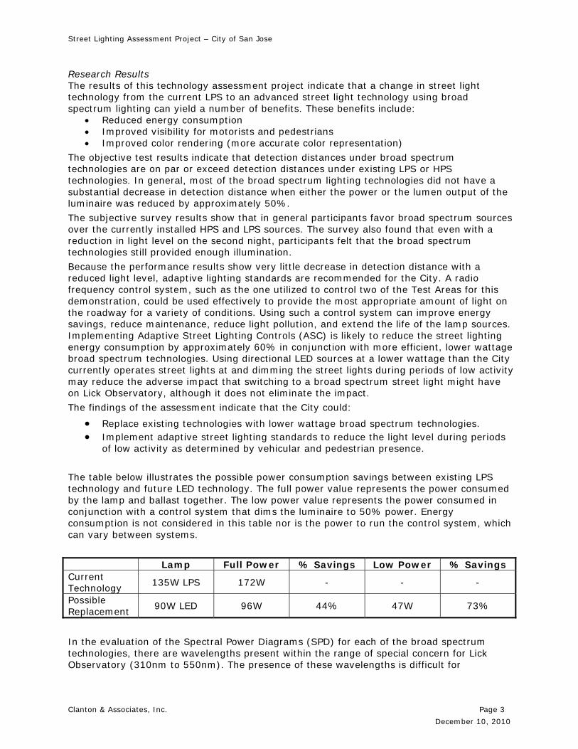
The table below illustrates the possible power consumption savings between existing LPS technology and future LED technology. The full power value represents the power consumed by the lamp and ballast together. The low power value represents the power consumed in conjunction with a control system that dims the luminaire to 50% power. Energy consumption is not considered in this table nor is the power to run the control system, which can vary between systems.
Lamp Full Power % Savings Low Power % Savings Current Technology
135W LPS 172W - - -
Possible Replacement
90W LED 96W 44% 47W 73%
In the evaluation of the Spectral Power Diagrams (SPD) for each of the broad spectrum technologies, there are wavelengths present within the range of special concern for Lick Observatory (310nm to 550nm). The presence of these wavelengths is difficult for

Street Lighting Assessment Project – City of San Jose
Clanton & Associates, Inc. Page 4
December 10, 2010
observatories to filter out because there are multiple peaks at varying wavelengths. The LPS works well for observatories because there is only one significant peak at a very narrow range of wavelengths. This makes it possible for the observatories to filter out the undesired wavelengths rather easily.
Installing lower wattage broad spectrum technology sources will reduce the overall light, but will add undesirable wavelengths for the observatory. Overall, it is anticipated that a complete change of LPS sources for LED sources could result in a 6.8% reduction in total terrestrial lighting power experienced as skyglow under full-power conditions. During times of 50% power reduction (due to low traffic volume), the complete change of LPS for LED sources could result in a 13.6% reduction in total terrestrial lighting power experienced as skyglow.
Street Lighting Assessment Project – City of San Jose
Clanton & Associates, Inc. Page 5
December 10, 2010
1.0 Introduction
The City of San Jose Advanced Street Lighting Assessment Project provides the City of San Jose with an evaluation of the energy savings potential of broad spectrum street lights provided by both light emitting diode (LED) and induction (IND) light sources, while maintaining critical characteristics required in a street lighting application. These characteristics include quality of light, aesthetics, maintenance, perceived public safety for pedestrians and motorists, and the environmental impact such as green house gases (GHG) from the generation of electricity to power the system. An additional consideration is the impact on the night sky and the astronomy community due to the proximity of Lick Observatory located atop Mount Hamilton 26 miles from downtown San Jose. The elevation gain from downtown San Jose to the observatory is approximately 4275 feet.
The specific goals and objectives of the project are:
1. Determine the energy reduction potential of advanced street light technologies, LED and IND, compared to the city standard low pressure sodium (LPS) and high pressure sodium (HPS) sources.
2. Evaluate the light characteristics of each technology to determine if a gain in energy efficiency is possible without a compromise in visual performance.
3. Identify lighting technologies that are suitable substitutions for LPS on a large scale. 4. Collect and analyze target detection distance data under the test area light sources
to assist in the understanding of the visual performance of various street lighting technologies.
5. Evaluate subjective opinions of citizens toward various light sources that may be suitable candidates for selection as replacement luminaires for the City of San Jose street lighting.
6. Identify parameters or characteristics of proposed technologies that may be critical in the technology evaluation process.
1.1 History and Background
The City of San Jose has implemented various pilot projects to evaluate the feasibility of LED technology. To evaluate various types of broad spectrum street light technology including LED and IND, the City began this particular assessment project to identify and evaluate advanced street light technology which can benefit the public with increased visibility through improved color rendition and energy savings.
This effort was based upon current lighting research that suggests that the human eye can better perceive objects in low light levels when the source spectrum is broad with both short and long wavelength light, commonly perceived as ‘white light’1 & 2. Metal halide (MH), IND, and LED technologies with a color rendering index (CRI) of 65 or greater more closely produce ‘white light’ than a typical HPS lamp (with a CRI of approximately 20), or LPS lamps (with a CRI of approximately 5). In previous research, broad spectrum light sources have been found to improve perception-reaction time by providing roadway users better peripheral vision3.
This assessment project builds upon the experience and lessons learned from previous broad spectrum street lighting conversion studies conducted in Alaska and Southern California. This type of project is unique because it includes both subjective public input and objective lighting evaluations using sophisticated data collection equipment. The test results will be part of a data set that will help evaluate the role of lamp spectral distribution and visibility under mesopic lighting conditions for such research as the revision of the Illuminating Engineering Society of North America’s (IESNA) TM-12-06 ‘Spectral Effects of Lighting on Visual Performance at Mesopic Light Levels’4.
The human visual system works at different levels given the amount of visible light available for processing by our eyes. During normal daylight hours, the human visual system works on

Street Lighting Assessment Project – City of San Jose
Clanton & Associates, Inc. Page 6
December 10, 2010
a photopic level which allows for color perception using the cone receptors of the eye. Under extremely low light conditions, the eye uses scotopic vision; this uses the rod receptors of the eye. Mesopic light levels occur in between the two and uses a mixture of both cone and rod receptors at different levels. Roadway lighting usually fits into the mesopic luminance range which utilizes both types of receptors in the eye. Figure 1 below illustrates the approximate ranges of scotopic, mesopic, and photopic on a logarithmic scale of illumination in Lux.
Figure 1: Scotopic, Mesopic and Photopic Ranges5
1.2 Technology and Market Overview
New street lighting technologies have the potential benefits of improved efficiency, better maintenance characteristics, and improved control capabilities that can reduce the energy consumption and maintenance costs for an overall net gain for the City of San Jose. Broad spectrum technologies also have the potential for improved visual performance and preferred visual aesthetic that can result in an unquantifiable but appreciable public benefit as well.
The information gathered through this project will provide direction to the City of San Jose for future street lighting applications. It also provides a demonstration of a radio frequency control system. The publication of this project can provide insight for planning departments into public perception and nighttime visibility variables worth considering.
While research has been ongoing for sometime on the relationship between broad spectrum sources and impacts on human vision, the application to street and roadway lighting is early in development. This research is part of an increasing body of knowledge that will impact the IESNA recommendations for roadway lighting, and ultimately greatly impact the design practices of the lighting engineering community as a whole.
1.3 Prior Work
Previous studies of LED luminaires in the United States have been conducted by the Department of Energy (DOE) in Portland, Oregon; Minneapolis, Minnesota; and Oakland and San Francisco, California. These studies evaluated LED luminaires in residential neighborhoods and small street sections and focused primarily on energy consumption and economic performance.
The DOE studies contacted residents to see if they noticed the new lighting and if so, residents were asked to provide preference feedback from them. The study did not take participants through the test site to assess their preferences in an unbiased direct comparison manner. None of these studies included the objective visibility component used in San Jose to simulate driving and study target detection performance.
Clanton & Associates and the Virginia Tech Transportation Institute (VTTI) performed similar subjective and objective performance surveys recently for the Municipality of Anchorage6 and the City of San Diego7. The study in Anchorage included the evaluation of luminaires at two

Street Lighting Assessment Project – City of San Jose
Clanton & Associates, Inc. Page 7
December 10, 2010
different light levels in an effort to test the proof of concept for Adaptive Street Lighting Controls (ASC). The San Diego demonstration evaluated broad spectrum sources at one light level only.
Street Lighting Assessment Project – City of San Jose
Clanton & Associates, Inc. Page 8
December 10, 2010
2.0 Project Methodology
This project consists of an energy evaluation, a subjective survey, and an objective ‘performance’ survey to collect quantitative data. The energy evaluation was performed by taking power measurements of the street lighting systems and the expected hours of operation to model typical energy use totals for the year. The subjective survey portion was meant to determine community acceptance of broad spectrum light sources. The objective portion was meant to determine visibility performance for the broad spectrum sources through the use of Small Target Visibility (STV) style targets. Both the subjective and objective portions are meant to provide insight into the functional visibility provided by various lighting systems and the public preferences for these technologies.
2.1 Overall Project Setup
The test location consists of a four lane roadway with a raised median in an industrial and business park area along Hellyer Avenue in the City of San Jose. The roadway is relatively flat with several curves throughout the testing area.
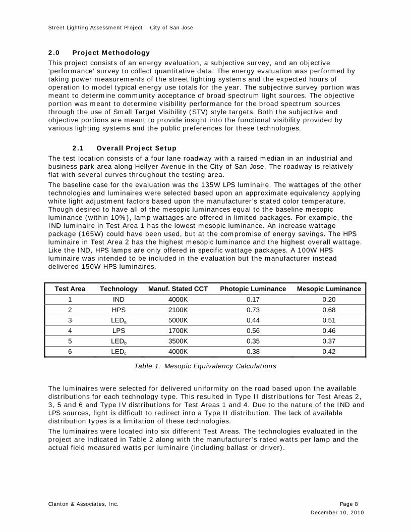
The baseline case for the evaluation was the 135W LPS luminaire. The wattages of the other technologies and luminaires were selected based upon an approximate equivalency applying white light adjustment factors based upon the manufacturer’s stated color temperature. Though desired to have all of the mesopic luminances equal to the baseline mesopic luminance (within 10%), lamp wattages are offered in limited packages. For example, the IND luminaire in Test Area 1 has the lowest mesopic luminance. An increase wattage package (165W) could have been used, but at the compromise of energy savings. The HPS luminaire in Test Area 2 has the highest mesopic luminance and the highest overall wattage. Like the IND, HPS lamps are only offered in specific wattage packages. A 100W HPS luminaire was intended to be included in the evaluation but the manufacturer instead delivered 150W HPS luminaires.
Table 1: Mesopic Equivalency Calculations
The luminaires were selected for delivered uniformity on the road based upon the available distributions for each technology type. This resulted in Type II distributions for Test Areas 2, 3, 5 and 6 and Type IV distributions for Test Areas 1 and 4. Due to the nature of the IND and LPS sources, light is difficult to redirect into a Type II distribution. The lack of available distribution types is a limitation of these technologies.
The luminaires were located into six different Test Areas. The technologies evaluated in the project are indicated in Table 2 along with the manufacturer’s rated watts per lamp and the actual field measured watts per luminaire (including ballast or driver).
Test Area Technology Manuf. Stated CCT Photopic Luminance Mesopic Luminance
1 IND 4000K 0.17 0.20
2 HPS 2100K 0.73 0.68
3 LEDa 5000K 0.44 0.51
4 LPS 1700K 0.56 0.46
5 LEDb 3500K 0.35 0.37
6 LEDc 4000K 0.38 0.42

Street Lighting Assessment Project – City of San Jose
Clanton & Associates, Inc. Page 9
December 10, 2010
Table 2: Lighting System Power Consumption
The Test Areas were located on a uniform stretch of roadway oriented Northwest-Southeast, with a uniform width and a typical cross-section of a shoulder on the South, two drive lanes going South, a median ranging from 6 to 16 feet, two drive lanes going North, and a shoulder on the North side. A setback sidewalk is located on the North side of the street. Figure 2 shows an aerial view of Hellyer Avenue and where the six Test Areas are located.
Figure 2: Experiment Location and Set-Up for Entire Test Area.
The poles are spaced approximately 160’ apart (to the next pole) in a roughly paired arrangement. Due to the curves in the road, this paired arrangement becomes more staggered for certain test areas.
2.2 Light Sources and Luminaires Light sources are commonly characterized by their color temperature and color rendering ability. Correlated Color Temperature (CCT, stated in Kelvin) identifies the ‘warmness’ or ‘coolness’ of the light color. A CCT of 2700K represents a warm incandescent-looking light. As the temperature increases, it represents a cooler light; a source rated at 5500K or 6500K appears somewhat blue compared to a 2700K source. Normal noon day sunlight has a typical CCT of 5000K. Northern blue sky has a CCT of 10,000 – 20,000K. Moonlight has a CCT of 4100K.
Test Area Technology Rated Power Watts/Lamp Actual Power Watts/Luminaire
1 IND 100 W 112 W
2 HPS 150 W 169 W
3 LEDa 98 W 98 W
4 LPS 135 W 172 W
5 LEDb 144 W 144 W
6 LEDc 96 W 96 W
North
Street Lighting Assessment Project – City of San Jose
Clanton & Associates, Inc. Page 10
December 10, 2010
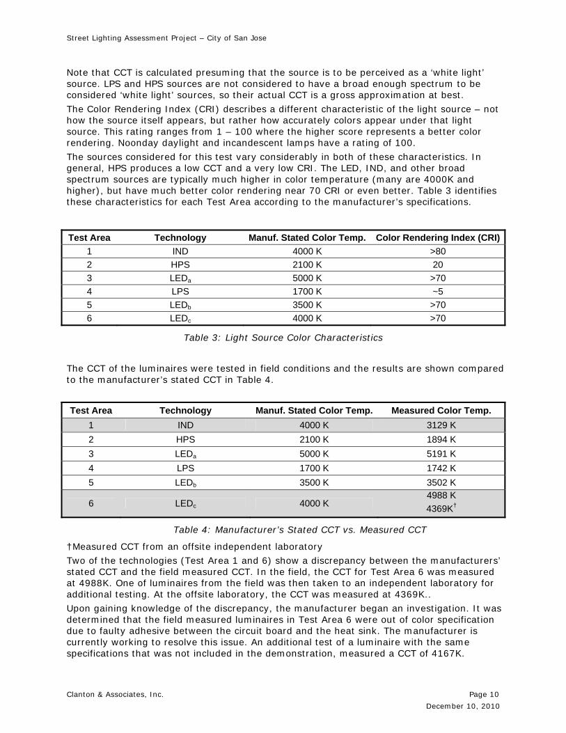
Note that CCT is calculated presuming that the source is to be perceived as a ‘white light’ source. LPS and HPS sources are not considered to have a broad enough spectrum to be considered ‘white light’ sources, so their actual CCT is a gross approximation at best.
The Color Rendering Index (CRI) describes a different characteristic of the light source – not how the source itself appears, but rather how accurately colors appear under that light source. This rating ranges from 1 – 100 where the higher score represents a better color rendering. Noonday daylight and incandescent lamps have a rating of 100.
The sources considered for this test vary considerably in both of these characteristics. In general, HPS produces a low CCT and a very low CRI. The LED, IND, and other broad spectrum sources are typically much higher in color temperature (many are 4000K and higher), but have much better color rendering near 70 CRI or even better. Table 3 identifies these characteristics for each Test Area according to the manufacturer’s specifications.
Test Area Technology Manuf. Stated Color Temp. Color Rendering Index (CRI)
1 IND 4000 K >80
2 HPS 2100 K 20
3 LEDa 5000 K >70
4 LPS 1700 K ~5
5 LEDb 3500 K >70
6 LEDc 4000 K >70
Table 3: Light Source Color Characteristics
The CCT of the luminaires were tested in field conditions and the results are shown compared to the manufacturer’s stated CCT in Table 4.
Test Area Technology Manuf. Stated Color Temp. Measured Color Temp.
1 IND 4000 K 3129 K
2 HPS 2100 K 1894 K
3 LEDa 5000 K 5191 K
4 LPS 1700 K 1742 K
5 LEDb 3500 K 3502 K
6 LEDc 4000 K 4988 K
4369K†
Table 4: Manufacturer’s Stated CCT vs. Measured CCT
†Measured CCT from an offsite independent laboratory
Two of the technologies (Test Area 1 and 6) show a discrepancy between the manufacturers’ stated CCT and the field measured CCT. In the field, the CCT for Test Area 6 was measured at 4988K. One of luminaires from the field was then taken to an independent laboratory for additional testing. At the offsite laboratory, the CCT was measured at 4369K..
Upon gaining knowledge of the discrepancy, the manufacturer began an investigation. It was determined that the field measured luminaires in Test Area 6 were out of color specification due to faulty adhesive between the circuit board and the heat sink. The manufacturer is currently working to resolve this issue. An additional test of a luminaire with the same specifications that was not included in the demonstration, measured a CCT of 4167K.
Street Lighting Assessment Project – City of San Jose
Clanton & Associates, Inc. Page 11
December 10, 2010
For LED luminaires, it is important to note the compromise that is experienced between CCT and efficacy (lumens per watt). Table 5 shows the three different LED luminaires that were included in this assessment. The highest efficacy is a result of LEDa, which also has the highest CCT. Currently, the lighting technology industry is experiencing an efficacy penalty for LEDs with lower CCTs. As LED technologies advance, the penalty is expected to diminish though unlikely to completely dissolve.
Test Area
Technology System Wattage Manuf. Stated Color Temp. Lumens Efficacy (lm/W)
3 LEDa 98 W 5000 K 6675 68.1
5 LEDb 144 W 3500 K 5558 38.6
6 LEDc 96 W 4000 K 5679 59.2
Table 5: Relationship between CCT and Efficiency for LED Luminaries
2.3 Multiple Light Levels
The study also evaluates the various lighting technologies at two different light levels: full and low. This effort was intended to evaluate the concept of adaptive lighting standards and determine the effect (subjectively and objectively) of reduced light levels at lower volume conditions during the nighttime.
To accommodate multiple light levels, a control system was selected and installed that communicated over radio frequency. With the exception of the LPS luminaires, each luminaire was intended to be equipped with a fully dimmable driver. Additional control devices were installed in the luminaires to wirelessly connect the driver with a base station located at the test site. With an internet connection and laptop, a programmer can turn on and off and dim each of the luminaires independently. All of the technologies (except the LPS) were configured for use with the control system. However, due to a variety of issues, including logistics and time constraints, only two of the luminaire manufacturers were integrated with the control system.
Three of the manufacturers were controlled manually by theater gel to reduce the luminous output of the sources to a low setting. Two manufacturers were controlled through the radio frequency network control system that reduced their power by half. Test Area 4 (LPS) operated at full power and output both nights of the assessment. On the first night of the assessment, the luminaires were evaluated at the full setting. The second night, the luminaires were evaluated at the low setting.
2.3.1 Output
To simulate a dimmed state, a neutral density theater gel was applied to the lens of each of the luminaires in Test Area 1 (IND), Test Area 2 (HPS) and Test Area 3 (LEDa). Because of the individual characteristics of each lamp source and luminaire manufacturer, the theatre gel applied a varying percentage of transparency to each Test Area, which was approximately 50%.
The low values are not the absolute measurement of the luminaires at low output. The values are field measurements based upon the mean illuminance, therefore, are subject to field condition errors. Table 6 shows the number of lumens for each Test Area at full and low settings. The percentages of full values represent the percent reduction in light output (lumens) at the low setting. These values were calculated using the illuminance measurements performed by Virginia Tech Transportation Institute (VTTI) in the field.

Street Lighting Assessment Project – City of San Jose
Clanton & Associates, Inc. Page 12
December 10, 2010
Test Area Technology Full (lumens) Low (lumens) % of Full
1 IND 5695 3589 63%
2 HPS 12,240 5563 45%
3 LEDa 6675 4405 66%
4 LPS 12,076 12,076 100%
5 LEDb 5558 4429 79%
6 LEDc 5679 3550 63%
Table 6: Estimated Lumen Output at Full and Low Settings
2.3.2 Power
Two of the Test Areas with dimming capabilities installed were controlled via the radio frequency control system. The low setting was accomplished by dimming each of the luminaires in Test Area 5 (LEDb) and Test Area 6 (LEDc) by reducing the input power by 50%. Test Areas 1, 2 and 3 were not reduced based upon power. Therefore, the percentage of full power for Test Areas 1, 2, and 3 is based upon an approximate relationship between output and power. These relationships are different for each technology. The relationships will vary depending on the output/power level that the luminaires are reduced to either manually or automatically by a control system.
Test Area Technology Full System Power Low System Power % of Full
1 IND 112W 67W 60%*
2 HPS 169W 93W 55%*
3 LEDa 98W 62W 63%*
4 LPS 172W 172W 100%
5 LEDb 144W 75W 52%
6 LEDc 96W 47W 49%
*Predicted value
Table 7: Estimated Power Consumption at Full and Low Settings
2.4 Lighting Calculations
Prior to the field assessment, in house computer simulated models were created. It is expected that these models differ from the field calculations due to other contributors of light in the field and the raised measurement plane. The in house calculations simulated illuminance values at the ground plane. The calculated light levels for Test Areas 2 and Test Area 5 are shown in false-color diagrams below. These diagrams are illustrating the full light level setting representing the first night of the assessment. The diagrams for the other Test Areas can be found in Appendix E: Site Calculations. The scale is the same for all diagrams, therefore relative comparisons of the light levels on the street may be made with a reasonable measure of accuracy. The calculations are based upon typical luminaire spacing 160’ pole-to-pole. The false-color rendering for Test Areas 2 and 5 are shown below in Figure 3 and Figure 4, respectively.

Street Lighting Assessment Project – City of San Jose
Clanton & Associates, Inc. Page 13
December 10, 2010
Figure 3: False-Color Rendering for Test Area 2 – Typical Spacing of 160’
Figure 4: False-Color Rendering for Test Area 5 – Typical Spacing of 160’
Scale: Illuminance (FC)
0 0.5 1 1.5 The diagrams above provide context for the calculated light levels that are delivered by the different lighting systems tested with the use of colors instead of values. The distribution of the light to each side of the luminaire and across the road is represented with these diagrams, and the distribution from high point to the low points can be understood as well.
For example, consider the information presented in the above diagrams. Test Area 2 shows higher ‘high’ values compared to Test Area 5 which shows lower ‘high’ values and lower ‘low’ values. While average illuminance is not directly shown on the diagrams, it is clear that Test Area 5 has the lower average due to the preponderance of the lower values throughout the measurement area. The light distribution from the two test areas is also quite different. Test Area 2 has a wider distribution than Test Area 5.
Street Lighting Assessment Project – City of San Jose
Clanton & Associates, Inc. Page 14
December 10, 2010
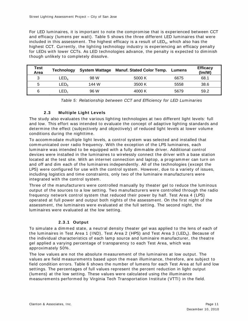
Additionally, each Test Area was measured for total efficiency actually hitting the roadway. This calculation is based upon typical spacing of the luminaires. Of all the downward directed light, only a portion (Figure 5) hits the road surface and is utilized directly from the primary task of street lighting. All uplight from a streetlight is considered non-useful and should be avoided (Figure 6).
Figure 5: Plan View of Luminaire Distribution and Highlighted Roadway Surface
Figure 6: Isometric View of Luminaire Uplight Distribution
In order to arrive at the value for total efficiency actually hitting the roadway, a series of intermediate calculations are performed. Using a computer simulated model, an average value for the illuminance (FC) reaching only the roadway is calculated. This calculation accounts for the luminaire efficiency. The average illuminance reaching the roadway is then multiplied by the area of the roadway. This calculation determines the amount of roadway lumens directly hitting the surface of the roadway. The Lamp Roadway Efficiency is determined by taking the number of lumens actually hitting the roadway and dividing by the initial lamp lumens. This calculated value is the percentage of the total output of the lamp delivered to the roadway surface. The Luminaire Roadway Efficiency is determined also by using the number of lumens actually hitting the roadway, but dividing by the luminaire lumens. This calculated value is the percentage of the total output of the luminaire delivered

Street Lighting Assessment Project – City of San Jose
Clanton & Associates, Inc. Page 15
December 10, 2010
to the roadway surface. Since LED technologies have the same value for lamp and luminaire lumens, the lamp roadway efficiency equals the luminaire roadway efficiency. The higher Luminaire Roadway Efficiency means that more lumens are effectively leaving the luminaire and hitting the roadway. Note the Test Areas with the highest Luminaire Roadway Efficiency are Test Areas 3, 5 and 6.
The lamp and luminaire efficacy calculations are also based upon the actual light hitting the roadway. Note that the traditional efficiency (total luminaire lumens divided by system wattage) will be higher than the efficacy calculations because all of the light output will be included, not just the output hitting the roadway surface.
Test Area
Lamp Wattage
System Wattage
Source Lamp
LumensLuminaire Lumens
Lamp Roadway Efficiency
Luminaire Roadway Efficiency
Lamp Road.
Efficacy (lm/W)
Lumin. Road.
Efficacy (lm/W)
1 100 112 IND 8500 5695 23.06% 34.42% 19.60 17.50
2 150 169 HPS 16000 12,240 28.59% 37.37% 30.49 26.90
3 90 98 LEDa 6675 6675 51.39% 51.39% 34.30 32.80
4 135 172 LPS 22500 12,076 16.70% 31.11% 27.83 21.84
5 146 144 LEDb 5558 5558 47.02% 47.02% 17.90 16.44
6 100 96 LEDc 5679 5679 57.53% 57.53% 36.30 32.12
Table 8: Typical Roadway Efficiency Calculations
It is important to note the Luminaire Roadway Efficiency column above. These values aim to illustrate how effective each source is at delivering light to where it is desired: the road. Although LEDs have fewer lumens, the efficiency values are higher than traditional sources because LEDs are more directional and aim those fewer lumens to the target road surface. Even with the LEDs having higher roadway efficiency values, there are still nearly half of the lumens missing the roadway, by either hitting the surface to the side, behind, or in front of the road.
2.5 Survey Approach
The project subjectively and objectively evaluated six different luminaire systems, including one system that is representative of the existing lighting conditions. On the first night, participants evaluated the test luminaires at the full setting. On the second night, participants evaluated the test luminaires at the low setting with the exception of the LPS system which remained at the full setting for both nights. The participants were unaware of the low setting characteristics until after completing the survey.
Subjective Evaluation:
1. Two groups of participants evaluated each Test Area filling out a thirteen-statement survey.
2. Statements were rated to evaluate the perception of safety of the lighting system, the preference for the ‘color’ of the light, and other general impressions of the lighting system.
3. The results were analyzed for statistically significant differences in response among the various test areas.

Street Lighting Assessment Project – City of San Jose
Clanton & Associates, Inc. Page 16
December 10, 2010
Objective ‘Performance’ Evaluation:
1. Some of the participants from the subjective survey groups rode in a vehicle that traveled through each test area (three participants at a time).
2. Participants pushed a ‘detection’ button when they identified a target along the side of the road.
3. Equipment on the car recorded its location, the target location, the luminous scene at the time the target was recognized, as well as the illuminance and luminance conditions along the roadway.
4. These results were analyzed to establish the average detection distance to the target under each of the lighting systems.
The results of the two evaluation methods were then compared to find correlations between how participants subjectively view the different lighting conditions and how the different lighting conditions objectively perform.
2.6 Subjective Survey
The subjective lighting survey that is used consists of thirteen statements which the participants rated on a 1-5 scale (strongly disagree to strongly agree, respectively). The survey was administered to two groups (one each night) of individuals comprised of two sub-groups each. The groups evaluated the street lighting in six different areas. Each night, contained approximately 26 and 30 individuals in each subgroup. The surveys were completed as the individuals rotated through the six areas in a specific order. Within each group, one sub-group started with Test Area 1 (IND) and proceeded in order: 1, 2, 3, 4, 5, 6 while the other sub-group started with Test Area 4 (LPS) and proceeded in order: 4, 5, 6, 1, 2, 3. Both groups rotated through the lighting order until returning to the test area they began with.
The following list of statements comprised the survey. See Appendix A: Subjective Lighting Survey Form for survey forms.
1. ‘It would be safe to walk here, alone, during daylight hours.’ 2. ‘It would be safe to walk here, alone, during darkness hours.’ 3. ‘The lighting is comfortable.’ 4. ‘There is too much light on the street.’ 5. ‘There is not enough light on the street.’ 6. ‘The light is uneven (patchy).’ 7. ‘The light sources are glaring.’ 8. ‘It would be safe to walk on the sidewalk here at night.’ 9. ‘I cannot tell the colors of things due to the lighting.’ 10. ‘The lighting enables safe vehicular navigation.’ 11. ‘I like the color of the light.’ 12. ‘I would like this style lighting on my city streets.’ 13. ‘How does the lighting in this area compare with the lighting of
similar San Jose city streets at night?’
2.7 Objective ‘Performance’ Visibility Test The subjective survey results provide feedback from the community on the general favorability of a lighting system, but a ‘performance’ test is necessary to establish that a lighting option is equivalent from a performance perspective. The ‘performance’ test incorporates a response metric (detection distance), illuminance and luminance metrics. The data collection process for these metrics is made possible by using and enhanced version of the VTTI lighting and Infrastructure Technology (LIT) group’s Roadway Lighting Mobile

Street Lighting Assessment Project – City of San Jose
Clanton & Associates, Inc. Page 17
December 10, 2010
Measurement System (RLMMS). The combined data capturing capability allowed the research team to continuously collect response data from participants in addition to lighting metrics.
2.8 Experimental Design The experimental design incorporates six lighting systems, five of which are alternative light sources installed for this assessment. An existing LPS installation is used as a control and comparison section. The experimental design uses detection distance as the primary dependent variable. In order to gather this information, the experimental design incorporates a number of different colored targets for participants to detect through the process of Small Target Visibility (STV). Additional independent variables include full and low output/power settings and the different CCT of alternative lighting technologies. Details of these variables are shown in Table 9.
Variable Description
Lighting 5 alternative light sources (LEDa, LEDb, LEDc, IND, and HPS), and the
existing LPS control condition
Output/Power Full and Low
Color Gray (17% reflectance), Green (17% reflectance), Blue (15%
reflectance), Red (12% reflectance), and Yellow (57% reflectance) targets
Table 9: Objective Testing Experimental Variable Descriptions.
2.9 Methods for Objective Testing 2.9.1 Participants
A total of 75 participants volunteered to be passengers for the objective portion of the project which took place in the data collection vehicle. There were 39 participants for Night 1 and 36 participants for Night 2. The participant pool contained both males and females aged 18 and older. It should be noted that gender and age were not controlled for this project, thus were not analyzed. A single trip through all of the Test Areas contained up to three passengers who detected visibility targets from their respective positions in the front or back seat of the vehicle.
2.9.2 Equipment
Beyond the lighting installations on the street, two specific pieces of equipment are required for the objective performance experiment. The first is a complex measurement system developed for measuring roadway lighting installations (RLMMS). The second are visibility targets which are detected by the participants.
2.9.3 Equipment - Roadway Lighting Mobile Measurement System (RLMMS)
The data collection equipment used during the experiment contained a variety of elements for collecting illuminance, luminance, color temperature and participant response data. The RLMMS was created by the LIT at the VTTI as a method for collecting roadway lighting data in addition to participant response data.
A specially designed ‘Spider’ apparatus that contains four waterproof Minolta illuminance detector heads was mounted horizontally onto the vehicle roof in such a way that two meters were positioned over the right and left wheel paths and the other two meters are placed

Street Lighting Assessment Project – City of San Jose
Clanton & Associates, Inc. Page 18
December 10, 2010
along the centerline of the vehicle. An additional vertically mounted illuminance meter was positioned in the vehicle windshield as a method to measure glare from the lighting installations. The waterproof detector heads and windshield mounted Minolta head were connected to separate Minolta T10 bodies that send data to the data collection laptop positioned in the trunk of the vehicle.
A NovaTel Global Positioning Device (GPS) is positioned at the center of the four roof mounted illuminance meters and attached to the ‘Spider’ apparatus. The GPS device is connected to the data collection box via USB and the vehicle latitude and longitude position data are incorporated into the overall data file.
Two separate video cameras are mounted on the vehicle windshield; one collects color images of the forward driving luminous scene and the second camera collects luminance only information of the forward driving scene. Each camera is connected to a standalone computer that is then connected to the data collection computer. The data collection computer is responsible for collecting illuminance, human response (reaction times), and GPS data and synchronizes the camera computer images with a common timestamp. Additional equipment inside the vehicle consists of individual button boxes for participant entered responses and a Controller Area Network (CAN) reader to collect vehicle network information.
Each component of the RLMMS is controlled by a specialized software program created in LabVIEW™. The entire hardware suite is synchronized through the software program and data collection rates are set at 20Hz. Video image capture rate is set at 3.75 frames per second (fps). The final output file used during the analysis contains a synchronization stamp, GPS information (e.g., Latitude, Longitude), input button presses, individual images from each of the cameras inside the vehicle, vehicle speed, vehicle distance, and the illuminance meter data from each of the Minolta T-10s (4 total).
Figure 7 below shows the experimental vehicle used for this assessment. Figure 8 shows the experimental vehicle and the ‘Spider’ apparatus with incorporated Minolta waterproof heads in addition to the GPS unit and cameras mounted inside the vehicle.
Figure 7: Experimental Vehicle with RLMMS Components.

Street Lighting Assessment Project – City of San Jose
Clanton & Associates, Inc. Page 19
December 10, 2010
Figure 8: RLMMS Components mounted on and inside a vehicle
2.9.4 Equipment - Visibility Targets Research has established a relationship between certain visibility metrics (luminance, illuminance, etc.) and the detection and avoidance of a small object on a roadway. The calculation of Small Target Visibility (STV) is a method to calculate this relationship. The STV method was selected for this study to evaluate participants detecting a small object in the roadway. It is expected that larger objects (e.g., pedestrians) would be detected quicker than these small objects, thus STV provides a minimum performance measure. It is important to remember that STV performance tasks are difficult; a participant has to identify a small object, recognize it is a target of interest and then react by pressing a button.
The STV method (as defined by IESNA RP-8)8 is used to determine the visibility level of an array of targets along the roadway when considering certain factors such as: the luminance of the targets, the luminance of the immediate background, the adaptation level of the adjacent surroundings, and the disability glare. The weighted average of the visibility level of these targets results in the STV value. STV is one means of measuring visibility performance of potential objects in the roadway.
The STV style targets are flat, vertical, wooden square targets, which measure 7 inches (~18 cm) on each side, with the surface painted. On one side, a tab is also located measuring 2.375 inches (6 cm) by 2.375 inches (6 cm) and provides a means for participants to distinguish a valid target from other potential objects on or near the roadway. There are five potential target colors: gray, blue, green, red and yellow with bases painted to be similar to the road surface. The targets are pictured in Figure 9. These objects were located along the roadway and were used as the objects of interest in the performance portion of the project.

Street Lighting Assessment Project – City of San Jose
Clanton & Associates, Inc. Page 20
December 10, 2010
Figure 9: Detection Targets used within Test Areas
Targets of each color were positioned within each of the Test Areas. Target positions with respect to luminaires varied based on the luminance levels, however all targets were positioned approximately 60 inches (152.4 cm) from the side of the gutter towards the center of the roadway.
The targets were placed in the outermost lane of the roadway in such a way as not to be struck by the participant vehicle. Locations of the targets positions are illustrated below in Figure 10. The color (GN=Green, GR= Gray, BL= Blue, R= Red, Y= Yellow) is also identified in the Figure along with the luminance value of the target. The targets were positioned in each Test Area with the intent to have equal luminance values. Luminance values were also normalized across different Test Areas. Because of the high reflectance of the yellow target, an equal luminance value was not achieved for this target color.
The entire test route containing each of the lighting areas is roughly 0.75 mi (1.2 km) in length. The roadway installations contain the same number of luminaires and the length of each area is comparable across lighting types.
Figure 10: Experiment Location and Set-Up for Test Areas 1 and 2
Yellow
Red Blue
Green Gray
North

Street Lighting Assessment Project – City of San Jose
Clanton & Associates, Inc. Page 21
December 10, 2010
Figure 11: Experiment Location and Set-Up for Test Areas 3 and 4
Figure 12: Experiment Location and Set-Up for Test Area 5 and 6
2.9.5 Contrast An important concept to understand when viewing targets and interpreting the data is contrast. Contrast is a measure of perceptual differences between an object and its background. Figure 13 shows the equation used to calculate a particular form of contrast: Weber Contrast. Using Weber Contrast, the contrast is calculated by the difference between the luminance of the object on interest (Lobject) and the luminance of the background (Lbackground) divided by the luminance of the background.
Figure 13: Weber Contrast Equation
North
North

Street Lighting Assessment Project – City of San Jose
Clanton & Associates, Inc. Page 22
December 10, 2010
The equation can produce values ranging from infinity to negative one. Thus, contrast can be both positive and negative. In Figure 14 for example, positive contrast is when an object is brighter than its background (e.g., left image). Conversely, negative contrast is when an object is darker than its background (e.g., right image). In the field, targets were not positioned to achieve equivalent contrast values within Test Areas because it was not possible due to differences in light output, pole spacing, and road and background conditions for each Test Area.
Figure 14: Positive (left) and Negative (right) Contrast
The Weber Contrast equation is used in the analysis of target detection explained in Section 4.4 Objective Visibility Analysis.
2.10 Survey Night Site Conditions
The weather on the first night of the survey was overcast. The roadway was wet from rain during the day and a light rain started towards the end of the survey. On the second night of the survey, the sky was partly cloudy. The roadway was dry and clear.
The entire test area was closed before the first survey and remained closed through the final survey group both nights. Participants were able to enter the roadway to make the assessments. However, due to the ongoing visibility test vehicle traveling the roadway, participants were advised to remain on the sidewalk and only step onto the road shoulder or into the roadway for brief periods. Most participants answered the survey statements from the setback sidewalk.
2.11 Photos
The team took photos of the experiment area on the night of the surveys.
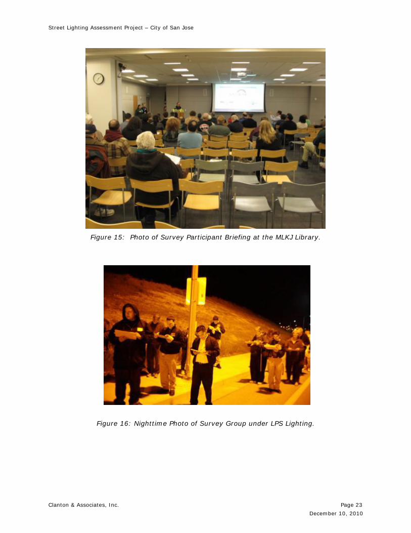
Street Lighting Assessment Project – City of San Jose
Clanton & Associates, Inc. Page 23
December 10, 2010
Figure 15: Photo of Survey Participant Briefing at the MLKJ Library.
Figure 16: Nighttime Photo of Survey Group under LPS Lighting.

Street Lighting Assessment Project – City of San Jose
Clanton & Associates, Inc. Page 24
December 10, 2010
Figure 17: Nighttime Photo of Survey Group under White Lighting.
2.12 Procedure
Participants were introduced to the subjective and objective assessment project at the meeting site in the City of San Jose. On the first night, participants met at the City’s Roosevelt Community Center; on the second night, at the Dr. Martin Luther King Jr. Library. Once the protocol and overview of the evening was complete, the participants were split into two groups and each was taken to a specific starting location on Hellyer Avenue. When the participants arrived at the testing site, the first three participants were then recruited for the driving portion of the study. The participants chose amongst themselves who sat in the front versus the back of the vehicle. The participants were then asked to enter the vehicle and review the tasks prior to starting this portion of the research study. In addition to the two testing groups of participants, there was also another group of industry professionals who participated in the objective portion of the study. Since these professionals have insight and knowledge in the industry of lighting, they did not participate in the subjective portion of the survey. While the other participants were being briefed each night, the industry professionals were on site participating in the objective portion of the survey.
While sitting in the stationary experimental vehicle, the detection task was reviewed by the in-vehicle experimenter. The experimenter pointed out the response buttons that were positioned both in the front and rear seats of the vehicle. The response buttons were to be pressed by the participants upon detecting a target object on the roadway. After the buttons were introduced, the participants were shown an example target.
Participants were instructed only to press a response button when they were confident that they had seen a target object. The participants were requested to notify the experimenter if a button had been pressed accidently during the experimental run.
Prior to beginning the experimental drive the participants in the back seat were also asked to move to where they could comfortably see the forward view of the roadway and thus detect targets out of the front windshield (rather than the side windows). Each participant was asked not to converse or hint to the other participants when they had seen a target in order to minimize influencing detection distances. Prior to starting the experimental run, the experimenter asked if the participants had any questions or concerns regarding the detection task or what was being asked of them.
When all questions had been addressed, the experimenter then started recording a data collection file. If a target were present at or near the starting location the experimenter

Street Lighting Assessment Project – City of San Jose
Clanton & Associates, Inc. Page 25
December 10, 2010
marked the data so these targets would be ignored. The starting location of the experimental vehicle varied during the testing sessions and was dependent on the location of the subjective evaluation participants.
The vehicle was driven at a maximum speed of 35 mph, which was 10 mph below the designated road speed on that section of Hellyer Avenue. The 35 mph speed was selected as a typical speed for a commercial lighting roadway because it was felt that it was more representative of typical roadways than the posted 45 mph speed on Hellyer Avenue. The experimental vehicle also drove in the far left lane in each direction of travel. In additional to driving the vehicle, the in-vehicle experimenter also marked the data by pressing a keyboard button where the actual target locations existed. Along the route, the participants pressed buttons when they were confident they had detected the target objects located on the side of the roadway. The total testing time for the detection task lasted approximately 5 minutes. This was broken down by having the participants review the experiment (1 min) and then engage in the detection task as they were driven along the route (~ 4 min). A total of 13 runs were made the first night, with the participants drawn from both subjective evaluation groups that evening. On the second evening of testing a total of 12 runs were made through the testing sections, again with participants drawn from both subjective evaluation groups. At the end of the in-vehicle test session, the vehicle was then taken back to one of the subjective evaluation groups where the participants were dropped off and a new set of participants were picked up. At the end of the test each evening, participants were returned to the initial meeting site by bus and thanked for their participation. No compensation was given to participants for their participation.
2.13 Data Analysis Two separate data analyses were performed for visibility data and illuminance sensor data.
For the objective visibility analysis, an initial data cleaning was performed where targets were located via GPS coordinates, responses were verified and matched to each target section, and additional data anomalies (e.g., detection distances three times the mean) were removed from the data. An additional data check was then performed to look for any other outliers and to check the images associated with the data file. These were performed by checking the data in Arc Map and verifying the image information. Then the entire data file including the information captured from the participants, the latitude and longitude of where the actual target locations existed, and the respective image names from the color and luminance cameras was imported into a Statistical Analysis Software (SAS) for review and analysis. When the detection distance calculations were completed the dataset underwent an additional data check for outliers and anomalous data and corrections were made as required (e.g., either deletions for false button presses, frame corrections, or deletions for anomalous data). ANalysis of COVAriance (ANCOVA) was used as the statistical tool to investigate differences among lighting type, setting level (full or low), and target variables such as target color.
The objective illuminance data for the lighting sections underwent the same data cleaning process as the visibility data. The entire data file was checked for anomalies and sections were verified with GPS information. The cleaned data file was then imported into SAS for review and analysis. The illuminance data gave an approximation of the light intensity reaching the road surface. It is important to note the meters were attached to the roof of the vehicle approximately six feet above ground level, which gave a further understanding of the performance of the different lighting sections.

Street Lighting Assessment Project – City of San Jose
Clanton & Associates, Inc. Page 26
December 10, 2010
3.0 Results The following sections provide information on the results of the subjective and performance surveys, energy and cost implications, lighting field measurements, and lighting calculations. A comparison of energy savings is made here, assuming a one for one replacement for each of the luminaires in each of the Test Areas. Not all of the luminaires in each of the Test Areas are delivering the same mesopic luminance as currently delivered by the City’s standard 135W LPS, and therefore may not be considered a viable replacement for the existing lighting equipment.
3.1 Electrical Demand and Energy Savings The base case luminaire in Test Area 4 (LPS) has an average measured system wattage of 172W per luminaire. Based upon 4017 annual operating hours per year in San Jose, the estimated annual energy consumption for a single LPS luminaire is 691 kWh.
The average system wattage consumption for the broad spectrum street light technologies is 113 W for the LED luminaires and 112 W for the IND luminaires. The annual energy consumption for the LED is 454 kWh and the IND is 450 kWh. A discussion of the hours of operation with and without controls will be expanded upon in Section 4.1 Energy Implications.
Test Area Technology Manufacturer’s
Stated Lamp Wattage
Measured System Wattage at Full
Setting
Power Savings based on existing LPS power usage
1 IND 100 112 35%
2 HPS 150 169 2%
3 LEDa 98 98 43%
4 LPS 135 172 -
5 LEDb 144 144 16%
6 LEDc 96 96 44%
Table 10: Average Measured Power Data (Full Power)
Test Area Technology Measured System
Wattage at Full Setting
Measured System Wattage at Low
Setting
Power Savings based on existing LPS power usage
1 IND 112 67* 61%*
2 HPS 169 93* 46%*
3 LEDa 98 62* 64%*
4 LPS 172 172 -
5 LEDb 144 75 56%
6 LEDc 96 47 73%
*Predicted values
Table 11: Average Measured Power Data (Low Power)
The power savings that is experienced at the low power setting is not a continuous, static savings. It is a predication for the possible savings that would be experienced during lengths of time where activity is reduced enough to dim the lights. An estimate for the composite

Street Lighting Assessment Project – City of San Jose
Clanton & Associates, Inc. Page 27
December 10, 2010
energy savings that is experienced over a typical year accounting for both periods of time at full and low power is found below in Table 12.

Street Lighting Assessment Project – City of San Jose
Clanton & Associates, Inc. Page 28
December 10, 2010
Test Area
Technology Measured System
Wattage at Full Setting
Estimated Annual Energy Consumption
(4017 hr/yr, kWh)
Estimated Annual Energy Savings based
upon existing LPS energy usage
1 IND 112 450 35%
2 HPS 169 679 2%
3 LEDa 98 394 43%
4 LPS 172 691 -
5 LEDb 144 578 16%
6 LEDc 96 386 44%
Table 12: Energy Consumption at Full Power
Test Area
Lamp Type
Measured System Wattage
(Full Setting)
Measured System Wattage
(Low Setting)
Hours of Op. per Year at
Full Power**
Hours of Op. per Year at
Low Power**
Annual Energy Consumption with Dimming
Controls (kWh)
Estimated Annual Energy Savings
1 IND 112 67* 321 53%
2 HPS 169 93* 462 33%
3 LEDa 98 62* 291 58%
4 LPS 172 172 691 0%
5 LEDb 144 75 382 45%
6 LEDc 96 47
1163 2854
246 64%
*Predicted values.
**Calculation of hours of operation is discussed more in 4.1 Energy Implications.
Table 13: Energy Consumption with Dimming Controls
The above calculations illustrate that an energy efficient broad spectrum luminaire has the potential to save between 16%-44% in power consumption alone at the full power setting. When at the low power setting, an energy efficient broad spectrum luminaire has the potential to save between 56%-73% in power consumption. When adaptive controls are implemented to reduce the power level to 50% during periods of low activity in conjunction with energy efficient luminaires, the energy consumption is reduced by 45%-64%.
3.2 Calculated Lighting Values 3.2.1 Illuminance Calculations
Table 14 shows illuminance calculations for all of the Test Areas, normalized to 160’ spacing pole-to-pole. This provides the possibility to compare the performance of the lighting systems on a level playing field, and shows additional information that is not possible to obtain in the field. These values were calculated under ideal conditions: full power/output, no other contributing light, and measured at the ground level. It is expected that these values will differ from those measured in the field.

Street Lighting Assessment Project – City of San Jose
Clanton & Associates, Inc. Page 29
December 10, 2010
Illuminance at Grade (FC)
Test Area Avg. Max. Min. Avg./ Min.
Max./ Min.
1 0.3 1.1 0.1 3.9 13.1
2 0.5 0.7 0.2 2.3 3.4
3 0.6 0.8 0.2 2.7 3.6
4 0.6 1.4 0.3 1.8 4.5
5 0.4 1.0 0.2 1.8 4.1
6 0.5 1.1 0.2 2.9 6.2
Table 14: Lighting Systems Calculations
Since the luminaires in each of the Test Areas were placed on existing poles that were designed to meet Illuminating Engineering Society of North America (IESNA) criteria set forth in 1964, it is not expected that the above illuminance calculations will meet the current IESNA criteria. It is also expected that the illuminance measurements taken in the field will not meet the current IESNA criteria because the measurements were taken at an elevated plane instead of at the ground level.
The current IESNA criterion is outlined in RP-8: Recommended Practice for Roadway Lighting. There are three methods of lighting design within RP-8, including the ‘Illuminance’ method, the ‘Luminance’ methods, and the ‘Small Target Visibility’ method. Similarly, the American Association of State Highway and Transportation Officials (AASHTO) uses the ‘Illuminance’ method and the ‘Luminance’ method within their documents for design criteria, referencing the methods and specific criteria limits from the IES RP-8 document9.
Let it be noted that IES is the leading authority on lighting standards. While many municipalities may have their own lighting standards, many derive or refer to IESNA standards.
3.2.2 Spectral Power Distribution Calculations
While in the field, spectral power distribution (SPD) measurements were also taken. This measurement is performed to determine the relative spectral power contained in each of the wavelengths comprising each lamp source. Figure 18 - Figure 23 give a relative idea of the magnitude of each wavelength. Note the spectral power is relative to each of the specific technologies, lumen package and manufacturer and cannot be compared against one another. In general, the range of specific concern for Lick Observatory is 310 nm to 550nm.
Because the field measured luminaires in Test Area 6 (LEDC) were operating out of color specification, an investigation took place headed by the manufacturer. It was determined that the adhesive between the circuit board and the heat sink created a filter effect and caused a CCT shift towards shorter wavelengths and reduced the overall light output. Due to this issue, the following SPD graphs (Test Area 6 only) are not generated from the field collected data. Rather, additional independent laboratory testing was completed for a luminaire with the same specifications from the same manufacturer. The SPD data from this independent laboratory test is shown in the following diagrams instead of the field measured data.

Street Lighting Assessment Project – City of San Jose
Clanton & Associates, Inc. Page 30
December 10, 2010
0
0.1
0.2
0.3
0.4
0.5
0.6
0.7
0.8
0.9
1
380 430 480 530 580 630 680 730 780
Re
lati
ve
Sp
ect
ral P
ow
er
Wavelength (nm)
Figure 18: SPD of Test Area 1 (IND) Measured CCT 3129K
The SPD of Test Area 1 shows several peaks of significant magnitude in the range of special concern for Lick Observatory.
0
0.1
0.2
0.3
0.4
0.5
0.6
0.7
0.8
0.9
1
380 430 480 530 580 630 680 730 780
Re
lati
ve
Sp
ect
ral P
ow
er
Wavelength (nm)
Figure 19: SPD of Test Area 2 (HPS) Measured CCT 1894K
The SPD of Test Area 2 shows the peaks of magnitude toward the end of the range of special concern for Lick Observatory. While there are still some peaks present at the lower end of the range, they are smaller in relative comparison.

Street Lighting Assessment Project – City of San Jose
Clanton & Associates, Inc. Page 31
December 10, 2010
0
0.1
0.2
0.3
0.4
0.5
0.6
0.7
0.8
0.9
1
380 430 480 530 580 630 680 730 780
Re
lati
ve
Sp
ect
ral P
ow
er
Wavelength (nm)
Figure 20: SPD of Test Area 3 (LEDa) Measured CCT 5191K
The SPD of Test Area 3 shows its most significant peak within the range of special concern for Lick Observatory. There are a few other peaks that occur in the range.
0
0.1
0.2
0.3
0.4
0.5
0.6
0.7
0.8
0.9
1
380 430 480 530 580 630 680 730 780
Re
lati
ve
Sp
ect
ral P
ow
er
Wavelength (nm)
Figure 21: SPD of Test Area 4 (LPS) Measured CCT 1742K
The SPD of Test Area 4 has a very significant peak out of the range of special concern for Lick Observatory. Additionally, it is a monochromatic source (only one significant peak and a narrow range of wavelengths) so it can be specifically filtered out if needed.
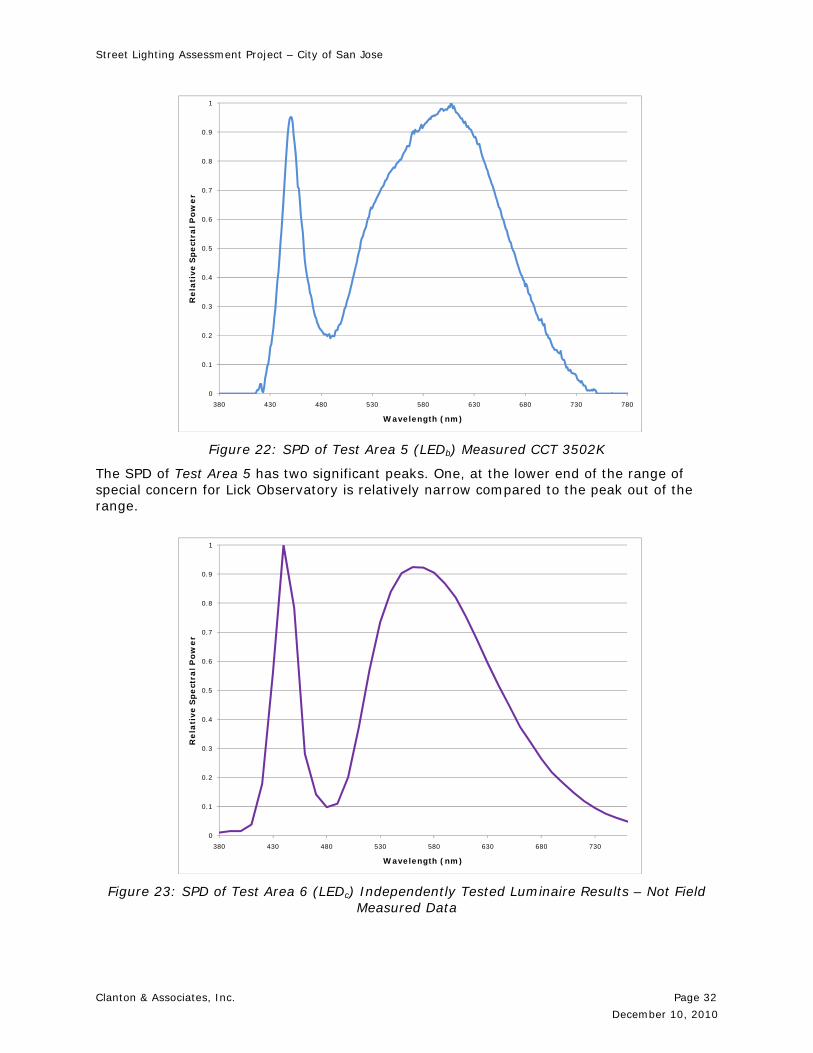
Street Lighting Assessment Project – City of San Jose
Clanton & Associates, Inc. Page 32
December 10, 2010
0
0.1
0.2
0.3
0.4
0.5
0.6
0.7
0.8
0.9
1
380 430 480 530 580 630 680 730 780
Re
lati
ve
Sp
ect
ral P
ow
er
Wavelength (nm)
Figure 22: SPD of Test Area 5 (LEDb) Measured CCT 3502K
The SPD of Test Area 5 has two significant peaks. One, at the lower end of the range of special concern for Lick Observatory is relatively narrow compared to the peak out of the range.
0
0.1
0.2
0.3
0.4
0.5
0.6
0.7
0.8
0.9
1
380 430 480 530 580 630 680 730
Re
lati
ve
Sp
ect
ral P
ow
er
Wavelength (nm)
Figure 23: SPD of Test Area 6 (LEDc) Independently Tested Luminaire Results – Not Field Measured Data
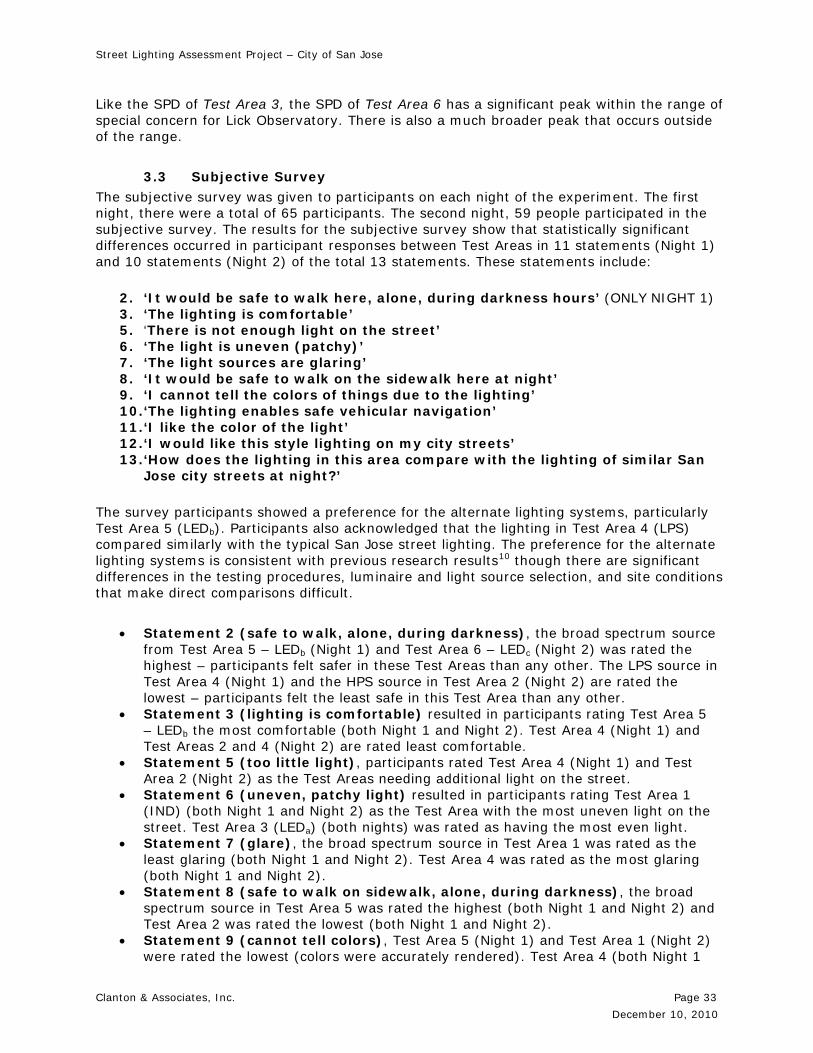
Street Lighting Assessment Project – City of San Jose
Clanton & Associates, Inc. Page 33
December 10, 2010
Like the SPD of Test Area 3, the SPD of Test Area 6 has a significant peak within the range of special concern for Lick Observatory. There is also a much broader peak that occurs outside of the range.
3.3 Subjective Survey
The subjective survey was given to participants on each night of the experiment. The first night, there were a total of 65 participants. The second night, 59 people participated in the subjective survey. The results for the subjective survey show that statistically significant differences occurred in participant responses between Test Areas in 11 statements (Night 1) and 10 statements (Night 2) of the total 13 statements. These statements include:
2. ‘It would be safe to walk here, alone, during darkness hours’ (ONLY NIGHT 1) 3. ‘The lighting is comfortable’ 5. ‘There is not enough light on the street’ 6. ‘The light is uneven (patchy)’ 7. ‘The light sources are glaring’ 8. ‘It would be safe to walk on the sidewalk here at night’ 9. ‘I cannot tell the colors of things due to the lighting’ 10. ‘The lighting enables safe vehicular navigation’ 11. ‘I like the color of the light’ 12. ‘I would like this style lighting on my city streets’ 13. ‘How does the lighting in this area compare with the lighting of similar San
Jose city streets at night?’ The survey participants showed a preference for the alternate lighting systems, particularly Test Area 5 (LEDb). Participants also acknowledged that the lighting in Test Area 4 (LPS) compared similarly with the typical San Jose street lighting. The preference for the alternate lighting systems is consistent with previous research results10 though there are significant differences in the testing procedures, luminaire and light source selection, and site conditions that make direct comparisons difficult.
Statement 2 (safe to walk, alone, during darkness), the broad spectrum source from Test Area 5 – LEDb (Night 1) and Test Area 6 – LEDc (Night 2) was rated the highest – participants felt safer in these Test Areas than any other. The LPS source in Test Area 4 (Night 1) and the HPS source in Test Area 2 (Night 2) are rated the lowest – participants felt the least safe in this Test Area than any other.
Statement 3 (lighting is comfortable) resulted in participants rating Test Area 5 – LEDb the most comfortable (both Night 1 and Night 2). Test Area 4 (Night 1) and Test Areas 2 and 4 (Night 2) are rated least comfortable.
Statement 5 (too little light), participants rated Test Area 4 (Night 1) and Test Area 2 (Night 2) as the Test Areas needing additional light on the street.
Statement 6 (uneven, patchy light) resulted in participants rating Test Area 1 (IND) (both Night 1 and Night 2) as the Test Area with the most uneven light on the street. Test Area 3 (LEDa) (both nights) was rated as having the most even light.
Statement 7 (glare), the broad spectrum source in Test Area 1 was rated as the least glaring (both Night 1 and Night 2). Test Area 4 was rated as the most glaring (both Night 1 and Night 2).
Statement 8 (safe to walk on sidewalk, alone, during darkness), the broad spectrum source in Test Area 5 was rated the highest (both Night 1 and Night 2) and Test Area 2 was rated the lowest (both Night 1 and Night 2).
Statement 9 (cannot tell colors), Test Area 5 (Night 1) and Test Area 1 (Night 2) were rated the lowest (colors were accurately rendered). Test Area 4 (both Night 1
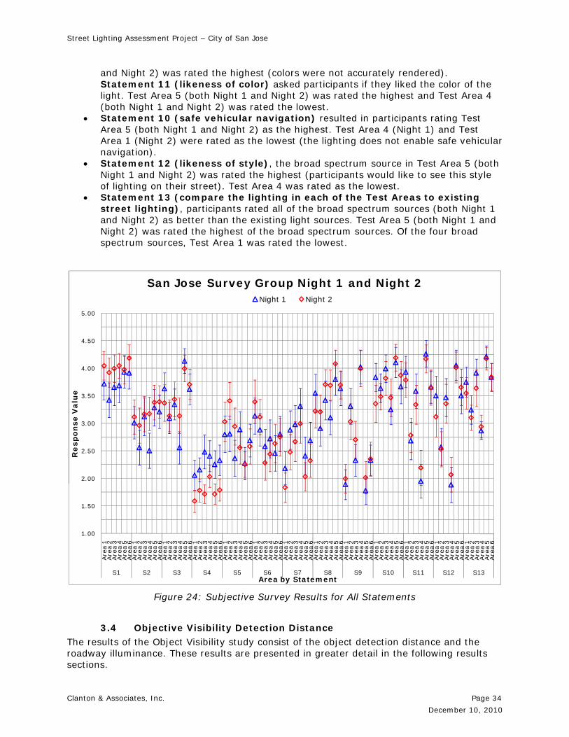
Street Lighting Assessment Project – City of San Jose
Clanton & Associates, Inc. Page 34
December 10, 2010
and Night 2) was rated the highest (colors were not accurately rendered). Statement 11 (likeness of color) asked participants if they liked the color of the light. Test Area 5 (both Night 1 and Night 2) was rated the highest and Test Area 4 (both Night 1 and Night 2) was rated the lowest.
Statement 10 (safe vehicular navigation) resulted in participants rating Test Area 5 (both Night 1 and Night 2) as the highest. Test Area 4 (Night 1) and Test Area 1 (Night 2) were rated as the lowest (the lighting does not enable safe vehicular navigation).
Statement 12 (likeness of style), the broad spectrum source in Test Area 5 (both Night 1 and Night 2) was rated the highest (participants would like to see this style of lighting on their street). Test Area 4 was rated as the lowest.
Statement 13 (compare the lighting in each of the Test Areas to existing street lighting), participants rated all of the broad spectrum sources (both Night 1 and Night 2) as better than the existing light sources. Test Area 5 (both Night 1 and Night 2) was rated the highest of the broad spectrum sources. Of the four broad spectrum sources, Test Area 1 was rated the lowest.
1.00
1.50
2.00
2.50
3.00
3.50
4.00
4.50
5.00
Are
a 1
Are
a 2
Are
a 3
Are
a 4
Are
a 5
Are
a 6
Are
a 1
Are
a 2
Are
a 3
Are
a 4
Are
a 5
Are
a 6
Are
a 1
Are
a 2
Are
a 3
Are
a 4
Are
a 5
Are
a 6
Are
a 1
Are
a 2
Are
a 3
Are
a 4
Are
a 5
Are
a 6
Are
a 1
Are
a 2
Are
a 3
Are
a 4
Are
a 5
Are
a 6
Are
a 1
Are
a 2
Are
a 3
Are
a 4
Are
a 5
Are
a 6
Are
a 1
Are
a 2
Are
a 3
Are
a 4
Are
a 5
Are
a 6
Are
a 1
Are
a 2
Are
a 3
Are
a 4
Are
a 5
Are
a 6
Are
a 1
Are
a 2
Are
a 3
Are
a 4
Are
a 5
Are
a 6
Are
a 1
Are
a 2
Are
a 3
Are
a 4
Are
a 5
Are
a 6
Are
a 1
Are
a 2
Are
a 3
Are
a 4
Are
a 5
Are
a 6
Are
a 1
Are
a 2
Are
a 3
Are
a 4
Are
a 5
Are
a 6
Are
a 1
Are
a 2
Are
a 3
Are
a 4
Are
a 5
Are
a 6
S1 S2 S3 S4 S5 S6 S7 S8 S9 S10 S11 S12 S13
Re
spo
nse
Valu
e
Area by Statement
San Jose Survey Group Night 1 and Night 2Night 1 Night 2
Figure 24: Subjective Survey Results for All Statements
3.4 Objective Visibility Detection Distance The results of the Object Visibility study consist of the object detection distance and the roadway illuminance. These results are presented in greater detail in the following results sections.
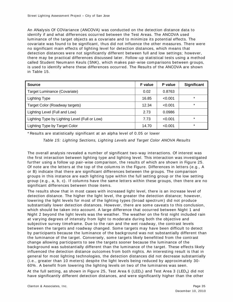
Street Lighting Assessment Project – City of San Jose
Clanton & Associates, Inc. Page 35
December 10, 2010
An ANalysis Of COVariance (ANCOVA) was conducted on the detection distance data to identify if and what differences occurred between the Test Areas. The ANCOVA used luminance of the target objects as a covariate and to minimize its potential effects. The covariate was found to be significant, thus did not influence the other measures. There were no significant main effects of lighting level for detection distances, which means that detection distances were not significantly different between full and low settings; however, there may be practical differences discussed later. Follow-up statistical tests using a method called Student Neumann Keuls (SNK), which makes pair-wise comparisons between groups, is used to identify where these differences occurred. The Results of the ANCOVA are shown in Table 15.
Source F value P value Significant
Target Luminance (Covariate) 0.02 0.8763
Lighting Type 16.85 <0.001 *
Target Color (Roadway targets) 12.34 <0.001 *
Lighting Level (Full and Low) 2.73 0.0986
Lighting Type by Lighting Level (Full or Low) 7.73 <0.001 *
Lighting Type by Target Color 14.70 <0.001 *
*Results are statistically significant at an alpha level of 0.05 or lower
Table 15: Lighting Sections, Lighting Levels and Target Color ANOVA Results
The overall analysis revealed a number of significant two-way interactions. Of interest was the first interaction between lighting type and lighting level. This interaction was investigated further using a follow up pair-wise comparison, the results of which are shown in Figure 25. Of note are the letters at the top of the columns in the Figure. Differences in letters (e.g., A or B) indicate that there are significant differences between the groups. The comparison groups in this instance are each lighting type within the full setting group or the low setting group (e.g., a, b, c). If columns have the same letters within these groups, then there are no significant differences between those items.
The results show that in most cases with increased light level, there is an increase level of detection distance. The higher the light level, the greater the detection distance; however, lowering the light levels for most of the lighting types (broad spectrum) did not produce substantially lower detection distances. However, there are some caveats to this conclusion, which should be taken into account. A large difference that occurred between Night 1 and Night 2 beyond the light levels was the weather. The weather on the first night included rain at varying degrees of intensity from light to moderate during both the objective and subjective survey timeframe. Due to the rain and the wet roadway, the contrast levels between the targets and roadway changed. Some targets may have been difficult to detect by participants because the luminance of the background was not substantially different than the luminance of the target. Conversely, some targets likely benefitted from the contrast change allowing participants to see the targets sooner because the luminance of the background was substantially different than the luminance of the target. These effects likely influenced the detection distance outcomes from both nights. An interesting result is that in general for most lighting technologies, the detection distances did not decrease substantially (i.e., greater than 10 meters) despite the light levels being reduced by approximately 30-60%. A benefit from lowering the lighting levels on two of the luminaires was seen.
At the full setting, as shown in Figure 25, Test Area 6 (LEDc) and Test Area 3 (LEDa) did not have significantly different detection distances, and were significantly higher than the other
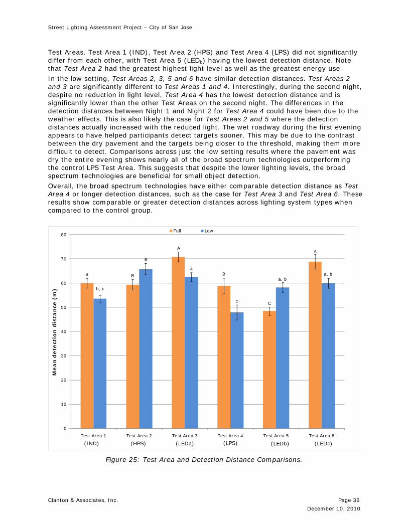
Street Lighting Assessment Project – City of San Jose
Clanton & Associates, Inc. Page 36
December 10, 2010
Test Areas. Test Area 1 (IND), Test Area 2 (HPS) and Test Area 4 (LPS) did not significantly differ from each other, with Test Area 5 (LEDb) having the lowest detection distance. Note that Test Area 2 had the greatest highest light level as well as the greatest energy use.
In the low setting, Test Areas 2, 3, 5 and 6 have similar detection distances. Test Areas 2 and 3 are significantly different to Test Areas 1 and 4. Interestingly, during the second night, despite no reduction in light level, Test Area 4 has the lowest detection distance and is significantly lower than the other Test Areas on the second night. The differences in the detection distances between Night 1 and Night 2 for Test Area 4 could have been due to the weather effects. This is also likely the case for Test Areas 2 and 5 where the detection distances actually increased with the reduced light. The wet roadway during the first evening appears to have helped participants detect targets sooner. This may be due to the contrast between the dry pavement and the targets being closer to the threshold, making them more difficult to detect. Comparisons across just the low setting results where the pavement was dry the entire evening shows nearly all of the broad spectrum technologies outperforming the control LPS Test Area. This suggests that despite the lower lighting levels, the broad spectrum technologies are beneficial for small object detection.
Overall, the broad spectrum technologies have either comparable detection distance as Test Area 4 or longer detection distances, such as the case for Test Area 3 and Test Area 6. These results show comparable or greater detection distances across lighting system types when compared to the control group.
B B
A
B
C
A
b, c
a
a
c
a, ba, b
0
10
20
30
40
50
60
70
80
Test Area 1 Test Area 2 Test Area 3 Test Area 4 Test Area 5 Test Area 6
Mea
n d
ete
ctio
n d
ista
nce
(m
)
Full Low
Figure 25: Test Area and Detection Distance Comparisons.
(IND) (HPS) (LEDc) (LEDb) (LPS) (LEDa)
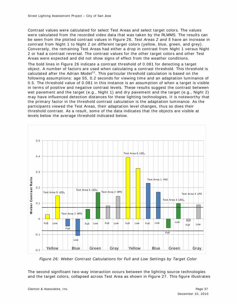
Street Lighting Assessment Project – City of San Jose
Clanton & Associates, Inc. Page 37
December 10, 2010
Contrast values were calculated for select Test Areas and select target colors. The values were calculated from the recorded video data that was taken by the RLMMS. The results can be seen from the plotted contrast values in Figure 26, Test Areas 2 and 5 have an increase in contrast from Night 1 to Night 2 on different target colors (yellow, blue, green, and grey). Conversely, the remaining Test Areas had either a drop in contrast from Night 1 versus Night 2 or had a contrast reversal. The contrast values for the other target colors and other Test Areas were expected and did not show signs of effect from the weather conditions.
The bold lines in Figure 26 indicate a contrast threshold of 0.081 for detecting a target object. A number of factors are used when calculating a contrast threshold. This threshold is calculated after the Adrian Model11. This particular threshold calculation is based on the following assumptions: age 55, 0.2 seconds for viewing time and an adaptation luminance of 0.5. The threshold value of 0.081 in this instance is an assumption of when a target is visible in terms of positive and negative contrast levels. These results suggest the contrast between wet pavement and the target (e.g., Night 1) and dry pavement and the target (e.g., Night 2) may have influenced detection distances for these lighting technologies. It is noteworthy that the primary factor in the threshold contrast calculation is the adaptation luminance. As the participants viewed the Test Areas, their adaptation level changes, thus so does their threshold contrast. As a result, some of the data indicates that the objects are visible at levels below the average threshold indicated below.
-0.2
-0.1
0
0.1
0.2
0.3
0.4
0.5
We
be
r C
on
tra
st
Ra
tio
Test Area 5 LEDb
Test Area 2 HPS
Test Area 5 LEDbTest Area 2 HPS
Test Area 6 LEDc
Test Area 1 IND
Test Area 3 LEDa
Test Area 4 LPS
Full
Full
Full Full Full Full
Full
FullLow
Low
Low Low Low Low LowLow
Figure 26: Weber Contrast Calculations for Full and Low Settings by Target Color
The second significant two-way interaction occurs between the lighting source technologies and the target colors, collapsed across Test Area as shown in Figure 27. This figure illustrates
Yellow Yellow Blue Blue Green Green Gray Gray
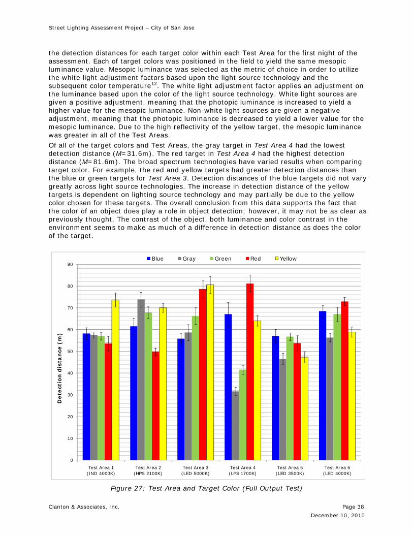
Street Lighting Assessment Project – City of San Jose
Clanton & Associates, Inc. Page 38
December 10, 2010
the detection distances for each target color within each Test Area for the first night of the assessment. Each of target colors was positioned in the field to yield the same mesopic luminance value. Mesopic luminance was selected as the metric of choice in order to utilize the white light adjustment factors based upon the light source technology and the subsequent color temperature12. The white light adjustment factor applies an adjustment on the luminance based upon the color of the light source technology. White light sources are given a positive adjustment, meaning that the photopic luminance is increased to yield a higher value for the mesopic luminance. Non-white light sources are given a negative adjustment, meaning that the photopic luminance is decreased to yield a lower value for the mesopic luminance. Due to the high reflectivity of the yellow target, the mesopic luminance was greater in all of the Test Areas.
Of all of the target colors and Test Areas, the gray target in Test Area 4 had the lowest detection distance (M=31.6m). The red target in Test Area 4 had the highest detection distance (M=81.6m). The broad spectrum technologies have varied results when comparing target color. For example, the red and yellow targets had greater detection distances than the blue or green targets for Test Area 3. Detection distances of the blue targets did not vary greatly across light source technologies. The increase in detection distance of the yellow targets is dependent on lighting source technology and may partially be due to the yellow color chosen for these targets. The overall conclusion from this data supports the fact that the color of an object does play a role in object detection; however, it may not be as clear as previously thought. The contrast of the object, both luminance and color contrast in the environment seems to make as much of a difference in detection distance as does the color of the target.
0
10
20
30
40
50
60
70
80
90
Test Area 1(IND 4000K)
Test Area 2(HPS 2100K)
Test Area 3(LED 5000K)
Test Area 4(LPS 1700K)
Test Area 5(LED 3500K)
Test Area 6(LED 4000K)
De
tect
ion
dis
tance
(m
)
Blue Gray Green Red Yellow
Figure 27: Test Area and Target Color (Full Output Test)

Street Lighting Assessment Project – City of San Jose
Clanton & Associates, Inc. Page 39
December 10, 2010
Since roadway lighting usually fits into mesopic luminance, there are implications on how to calculate the amount of light required on a roadway. These different levels (photopic, mesopic) can impact how we see objects in the roadway under different lighting conditions. An additional analysis was conducted based strictly on the gray targets in the experiment. The gray targets, dependent on direction of travel through the sections, were positioned as to have the same photopic or mesopic luminance levels. For example, the northwest travel direction had gray targets that were set at the same photopic levels and the southeast direction had gray targets set at the same mesopic level. These values were compared across Test Areas and the results are shown in Figure 28. Significant differences between the lighting types and target levels were achieved. When comparing across photopic levels, nearly all Test Areas had higher detection distances, except Test Area 2 and Test Area 3. This suggests that the target detection task benefitted by the placement of targets using the photopic calculations compared to the mesopic. Due to the manner in which the human eye views the targets, the findings suggest a benefit to using photopic calculations for all of the light source technologies.
A
B
B
A
B
A
b
a
b, c
d
c
b
0
10
20
30
40
50
60
70
80
90
Test Area 1 Test Area 2 Test Area 3 Test Area 4 Test Area 5 Test Area 6
Mea
n d
ete
ctio
n d
ista
nce
(m
)
Photopic Mesopic
Figure 28: Photopic and Mesopic Gray Target Detection Distance Comparisons
3.4.1 Weather Impacts on Detection Distance The weather did affect the detection distances of the targets each night of the assessment. Though all of the Test Areas except the control (Test Area 4 LPS) experienced a change in light level during the second night of the assessment, an unexpected change in contrast was also experienced. The change in contrast was not a result of changes to the lighting system,
(IND) (HPS) (LEDc) (LEDb) (LPS) (LEDa)

Street Lighting Assessment Project – City of San Jose
Clanton & Associates, Inc. Page 40
December 10, 2010
but rather a result of the differing weather conditions between the two nights of the evaluation.
It is not possible to normalize the data between the two nights to account for the impacts of weather resulting in contrast changes. It is however possible to normalize the data for each night separately to the performance of the control technology in Test Area 4. Figure 29 below illustrates the relative performance of all of the Test Areas compared to the control Test Area. Nearly all of the other technologies exceeded the detection distance of the control except for Test Area 5 (LEDb). Test Area 6 (LEDc) outperformed the control Test Area by the greatest amount.
0
0.2
0.4
0.6
0.8
1
1.2
1.4
Test Area 1 (IND)
Test Area 2 (HPS)
Test Area 3 (LEDa)
Test Area 4 (LPS)
Test Area 5 (LEDb)
Test Area 6 (LEDc)
Re
lati
ve
De
tect
ion
Dis
tan
ce
Figure 29: Relative Detection Distance Night 1 – Full Setting
For the second night (Figure 30), the data was also normalized to the performance of the control technology in Test Area 4. Even though all of the other Test Areas experienced an approximate 50% reduction in light level and the LPS did not experience any change in light level, all of the Test Areas outperformed the LPS. Test Area 2 (HPS) had the greatest detection distance relative to the LPS, though it also had the greatest light level and greatest energy use.

Street Lighting Assessment Project – City of San Jose
Clanton & Associates, Inc. Page 41
December 10, 2010
0
0.2
0.4
0.6
0.8
1
1.2
1.4
1.6
Test Area 1 (IND)
Test Area 2 (HPS)
Test Area 3 (LEDa)
Test Area 4 (LPS)
Test Area 5 (LEDb)
Test Area 6 (LEDc)
Re
lati
ve
De
tect
ion
Dis
tan
ce
Figure 30: Relative Detection Distance Night 2 – Low Setting
It is also useful to evaluate the relationship between the relative detection distance (normalized to the control LPS) and the watts per linear foot for each Test Area. Figure 31 below shows this relationship. As expected, Test Area 4 has one of the greatest power usages yet is outperformed by nearly all of the other Test Areas. Although Test Area 2 has the greatest energy use, the relative detection distance is only slightly higher than Test Area 4. A trend is visible for the broad spectrum technologies at the low setting where each consumes far less energy than the LPS, yet has a relatively higher detection distance than the LPS. Again, note the performance of the HPS at the low setting. Although having the greatest relative detection distance, the energy use is the greatest of the Test Areas that experienced a reduced light level.
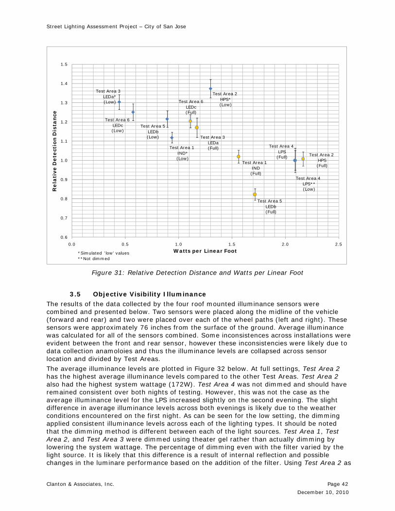
Street Lighting Assessment Project – City of San Jose
Clanton & Associates, Inc. Page 42
December 10, 2010
0.6
0.7
0.8
0.9
1.0
1.1
1.2
1.3
1.4
1.5
0.0 0.5 1.0 1.5 2.0 2.5
Re
lati
ve D
ete
ctio
n D
ista
nce
Watts per Linear Foot
Test Area 2HPS(Full)
Test Area 1IND(Full)
Test Area 4LPS
(Full)
Test Area 3LEDa(Full)
Test Area 5LEDb(Full)
Test Area 6LEDc(Full)
Test Area 6LEDc(Low)
Test Area 4LPS**(Low)
Test Area 3LEDa*(Low)
Test Area 5LEDb(Low)
Test Area 1IND*(Low)
Test Area 2HPS*(Low)
*Simulated 'low' values **Not dimmed
Figure 31: Relative Detection Distance and Watts per Linear Foot
3.5 Objective Visibility Illuminance The results of the data collected by the four roof mounted illuminance sensors were combined and presented below. Two sensors were placed along the midline of the vehicle (forward and rear) and two were placed over each of the wheel paths (left and right). These sensors were approximately 76 inches from the surface of the ground. Average illuminance was calculated for all of the sensors combined. Some inconsistences across installations were evident between the front and rear sensor, however these inconsistencies were likely due to data collection anamoloies and thus the illuminance levels are collapsed across sensor location and divided by Test Areas.
The average illuminance levels are plotted in Figure 32 below. At full settings, Test Area 2 has the highest average illuminance levels compared to the other Test Areas. Test Area 2 also had the highest system wattage (172W). Test Area 4 was not dimmed and should have remained consistent over both nights of testing. However, this was not the case as the average illuminance level for the LPS increased slightly on the second evening. The slight difference in average illuminance levels across both evenings is likely due to the weather conditions encountered on the first night. As can be seen for the low setting, the dimming applied consistent illuminance levels across each of the lighting types. It should be noted that the dimming method is different between each of the light sources. Test Area 1, Test Area 2, and Test Area 3 were dimmed using theater gel rather than actually dimming by lowering the system wattage. The percentage of dimming even with the filter varied by the light source. It is likely that this difference is a result of internal reflection and possible changes in the luminare performance based on the addition of the filter. Using Test Area 2 as

Street Lighting Assessment Project – City of San Jose
Clanton & Associates, Inc. Page 43
December 10, 2010
an example, the filter was placed on the flat glass surface of the luminaire. Light projected at low angles to reach the extents of the intensity distribution will both travel long distances through the filter itself as well as be more prone to total internal reflection issues. This will impact the uniformity and the overall performance of the luminaire and the roadway designs.
0
2
4
6
8
10
12
Test Area 1 (IND)
Test Area 2(HPS)
Test Area 3 (LEDa)
Test Area 4(LPS)
Test Area 5(LEDb)
Test Area 6(LEDc)
Test Area 1 (IND)
Test Area 2(HPS)
Test Area 3 (LEDa)
Test Area 4(LPS)
Test Area 5(LEDb)
Test Area 6(LEDc)
Full Settings Low Settings
Me
an
Ill
um
inan
ce L
evels
(Lu
x)
Figure 32: Mean Illuminance Levels per Test Area and Survey Night.
Table 16 below shows the average, minimum, and maximum illuminance values for each Test Area for each night of the assessment. Uniformity ratios are also included. In most cases the uniformity ratio increases at the low setting as expected. These values were obtained in the field from the roof mounted illuminance meters. Given the elevated plane (76 inches) which the meters were mounted, the values are not expected to meet the IESNA roadway lighting criteria.

Street Lighting Assessment Project – City of San Jose
Clanton & Associates, Inc. Page 44
December 10, 2010
Lighting Setting
Lighting Type
Average Illuminance
(lux)
Minimum Illuminance
(lux)
Maximum Illuminance
(lux)
Uniformity Ratio
(Max to Min)
Uniformity Ratio
(Avg to Min)Test Area 1
(IND) 8.9 0.27 66.08 244.75 33.26
Test Area 2 (HPS)
11.0 2.04 59.55 29.23 5.40
Test Area 3 (LEDa)
10.2 1.26 73.69 58.72 8.13
Test Area 4 (LPS)
8.2 1.33 27.64 20.86 6.18
Test Area 5 (LEDb)
8.3 0.58 100.96 174.06 14.36
Full
Test Area 6 (LEDc)
9.9 1.47 29.07 19.77 6.72
Test Area 1 (IND)
5.7 0.16 26.57 171.40 36.57
Test Area 2 (HPS)
5.0 0.46 28.04 61.62 10.99
Test Area 3 (LEDa)
6.8 1.44 17.05 11.86 4.74
Test Area 4 (LPS)
7.5 1.05 50.57 48.04 7.16
Test Area 5 (LEDb)
6.6 0.97 102.77 106.49 6.87
Low
Test Area 6 (LEDc)
5.3 0.58 22.37 38.39 9.02
Table 16: Maximum, Minimum, and Uniformity Calculations.
The fifth illuminance meter was located inside the vehicle and placed on the windshield. This meter provides a surrogate measure of the glare experienced while driving through each of the Test Areas. Slight differences between the full and low minimum illuminance levels for Test Areas 3 and 5 is likely influenced by the surrounding environment. Average illuminance levels were also calculated for each installation based on the ‘glare’ meter and the results are provided in Figure 33 below. Again, the information is categorized into the full and low settings. The glare readings for the full condition are comparable between Test Area 2, Test Area 6, and Test Area 3 which register between 8-9 lux. Again, there is little change between the LPS for each of the settings, suggesting the glare meter, measuring vertical illuminance, is less affected by the weather compared to the external horizontal illuminance meters. The overall results suggest that despite concerns about glare with the new lighting technologies, the majority of LEDs appear to have less glare consequences or are on par with the current lighting technologies.
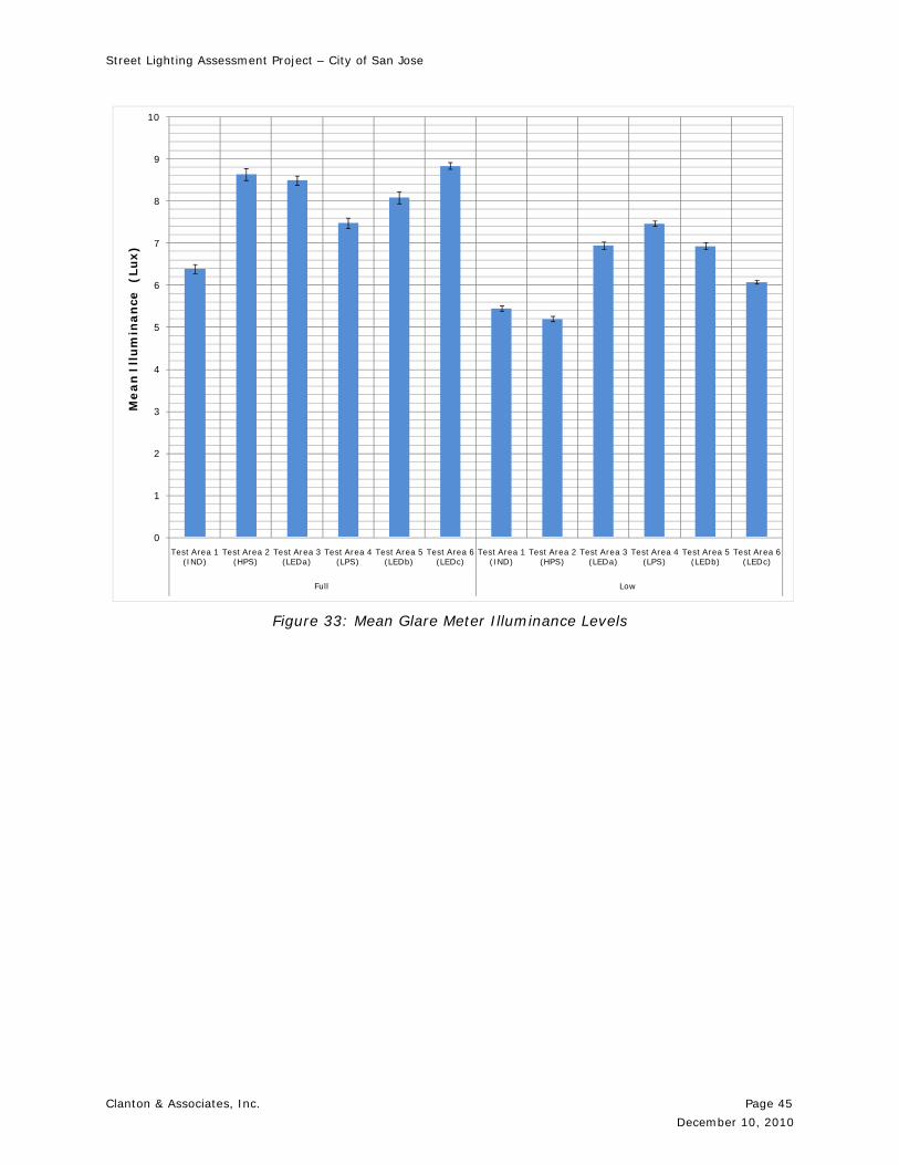
Street Lighting Assessment Project – City of San Jose
Clanton & Associates, Inc. Page 45
December 10, 2010
0
1
2
3
4
5
6
7
8
9
10
Test Area 1 (IND)
Test Area 2(HPS)
Test Area 3 (LEDa)
Test Area 4(LPS)
Test Area 5(LEDb)
Test Area 6(LEDc)
Test Area 1 (IND)
Test Area 2(HPS)
Test Area 3 (LEDa)
Test Area 4(LPS)
Test Area 5(LEDb)
Test Area 6(LEDc)
Full Low
Me
an
Ill
um
inan
ce
(Lux
)
Figure 33: Mean Glare Meter Illuminance Levels

Street Lighting Assessment Project – City of San Jose
Clanton & Associates, Inc. Page 46
December 10, 2010

Street Lighting Assessment Project – City of San Jose
Clanton & Associates, Inc. Page 47
December 10, 2010
4.0 Discussion
4.1 Energy Implications
The energy aspect of this project shows that there are some considerable possibilities to reduce energy consumption up to 60%, while still maintaining a comparable level of visual performance. There is a clear opportunity to reduce energy consumption and municipal tax dollars through a luminaire replacement program that shifts from the current LPS light sources to broad spectrum light sources.
The broad spectrum technologies discussed have considerably improved lamp life expectancy compared to the LPS or HPS technology light sources. This will result in a substantial improvement in maintenance periods, and reduction in overall expenses associated with this maintenance.
Due to the nature of LED light sources, the LED systems tested reflect different energy consumption partially because there are no ‘standard’ LED lamping packages. This will continue to be the case with LED as the industry advances.
However, one benefit of LED technology is the possibility that the lumen package can be adjusted to meet the needs of the roadway conditions more easily and in smaller increments than the traditional HPS or IND lamp wattage increments. This may result in the ability for a lighting designer to meet a standard without exceeding it too greatly; which will result in energy savings throughout the life of the lighting design, regardless of any other benefits that may be considered due to the broad spectrum nature of the light.
The energy savings predicted in Section 3.1 Electrical Demand and Energy Savings is calculated with a specific number of hours of street light operation for San Jose. The 4017 hours per year for a luminaire with no dimming controls is determined using Figure 32. This Figure shows the amount of daylight that San Jose receives throughout a typical year. The line near the top separating the daylight from nighttime is dusk and the line near the bottom separating nighttime from daylight is dawn. The horizontal axis is time in months of the year. The total hours of operation were determined summing the number of daylight hours during the summer, plus the number of daylight hours during the winter, plus the number of daylight hours during spring and fall. The total number of hours per year that a typical street light in San Jose, CA would operate is 4017, accounting for the lights coming on before dawn and turning off after dusk.

Street Lighting Assessment Project – City of San Jose
Clanton & Associates, Inc. Page 48
December 10, 2010
The reduced hours of operation per year that account for the luminaires to be dimmed a fraction of the time are illustrated in the following three graphs. These graphs are generated for the four seasons. In the winter, (Figure 35) there is less daylight, so the overall hours of operation are higher. As a preliminary scenario, it is estimated that during periods of low activity, street lights can be dimmed to 50% of total lumen output. The light color represents the amount of time during the day that the lights are operating under dimming controls. The dark color represents the savings that can be experienced with dimming controls. The same process can be used for the other seasons of the year. Adding together the number of hours that are at full power and the number of hours that are at 50% power, a composite 2592 equivalent hours per year is calculated.
Jan Feb Mar Apr May June July Aug Sep Oct Nov Dec
24
23 22 21
20 19 18 17 16 15 14
13 12 11 10 9 8 7 6
5 4 3 2 1
Hours
Figure 34: Typical Daylight Hours in San Jose, CA

Street Lighting Assessment Project – City of San Jose
Clanton & Associates, Inc. Page 49
December 10, 2010
00.10.20.30.40.50.60.70.80.9
1
0 1 2 3 4 5 6 7 8 9 10 11 12 13 14 15 16 17 18 19 20 21 22 23 24
Dim
ming Capability
Hours of the Day
Figure 35: Winter Street Lighting Use Profile
00.10.20.30.40.50.60.70.80.9
1
0 1 2 3 4 5 6 7 8 9 10 11 12 13 14 15 16 17 18 19 20 21 22 23 24
Dim
ming Capability (%)
Hours of the Day
Figure 36: Spring/Fall Street Lighting Use Profile
00.10.20.30.40.50.60.70.80.9
1
0 1 2 3 4 5 6 7 8 9 10 11 12 13 14 15 16 17 18 19 20 21 22 23 24
Dim
ming Capability (%)
Hours of the Day

Street Lighting Assessment Project – City of San Jose
Clanton & Associates, Inc. Page 50
December 10, 2010
Figure 37: Summer Street Lighting Use Profile

Street Lighting Assessment Project – City of San Jose
Clanton & Associates, Inc. Page 51
December 10, 2010
4.2 Street Lighting Dimming Controls The energy savings potential can be greatly increased through the application of an Adaptive Street Lighting Controls (ASC) system. This approach is beyond the scope of this project; however, it is an important technology to note. ASC is essentially advanced control for street lights. Each individual pole is given its own address that can be automatically controlled from a remote location. Based upon the needs of the City, additional levels of dimming control may be utilized. The benefits to considering adaptive lighting in a large scale municipal system of this kind include:
Reduced light pollution during the setback time periods.
Reduced energy consumption.
Longer lamp life.
Potential for demand response capability.
More sophisticated control and system management.
Improved maintenance information and truck routing.
A combination of both energy efficient broad spectrum technologies and an ASC system could result in energy consumption reductions of 60%. Savings are potentially increased due to improved information gathering, maintenance, and demand response potential.
4.3 Subjective Survey Analysis
The results do indicate a strong preference for broad spectrum sources compared to both the current LPS and the tested HPS light sources. Statement 11 shows the strength of this preference by grouping the four broad spectrum sources in a reasonably tight cluster and the two ‘yellow’ light sources (LPS and HPS) significantly below that level. The results indicate that white light sources will likely be accepted by the community should the City of San Jose choose an alternate source with broad spectrum light.
For Statement 3, (The lighting is comfortable), the respondents showed a substantial response difference between the existing LPS light sources and the others. The exception is the second night (when all but the LPS source were at low settings). That night, the LPS test area closed the gap upwards toward the rest of the test field considerably, and the others only slightly moved. This shift probably is a result of two factors; the first night had damp road surfaces, so reflected glare is a likely a source causing a down rating on the first night, and the second night had the LPS system at a higher light level than the rest, which may be interpreted by people as more favorable.
Statement 5 (There is not enough light on the street) produces a slightly different result. In this case, the respondents were mostly neutral on the first night, with some test areas slightly disagreeing and other test areas slightly agreeing. In most cases, the second night shows a shift toward agreeing with this statement with one exception: Test Area 4 (LPS). This test area was the same for both nights, but the rest of the Test Areas were lowered by approximately 50%.
The result of the light level shift is the respondents got ‘used to’ the light levels delivered by the dimmed systems, and when evaluating the LPS system sensed the higher light levels of the test area and therefore disagreed more with the statement that there was insufficient light in this test area.
Statement 6 (The light is uneven (patchy)) shows a general agreement that most of the Test Areas are not a problem feeling too uneven in light levels (uniformity ratios too high). The

Street Lighting Assessment Project – City of San Jose
Clanton & Associates, Inc. Page 52
December 10, 2010
worst scoring Test Area is Test Area 1. This indicates that there is possibly that the City has some flexibility with respect to the actual uniformity values that the public will accept.
Statement 7 (The light sources are glaring) shows several interesting issues. The first is that Test Area 4 is ranked the worst in this comparison. This is because the LPS fixture is not a flat lens styled full cutoff light source, so there is substantial light leaving the fixture in the primary glare zone (from about 75° to 90°). This result is expected.
The second result is the Test Area that is perceived as the least glare is Test Area 1 (IND). This is also expected, as the IND lamp is a large areas light source, and the brightness of the lamp is perceived by many people as much less glaring compared to LED light sources.
The third result is the LED Test Areas. While all of the LED test areas are somewhat similar in performance, of the two LED color temperatures that were tested (3500K and 5000K), participants rated the 3500K as less glaring than the 5000K. The differences in the scores for this test are not large, but the preference does appear to exist.
Statement 12 (I would like this style on my city streets) reinforces Statement 11 and shows that the broad spectrum light sources are all rated higher than the LPS or the HPS test areas. This is also an expected result, as most people have a preference for light sources that render accurately, and the broad spectrum sources will reflect this. As has occurred on several other Statements, the 3500K light source (Test Area 5) is rated the highest.
4.4 Objective Visibility Analysis The objective of the visibility analysis portion of the assessment was to analyze the impact of broad spectrum technologies with respect to visibility performance. This was achieved by a number of means which include having multiple targets of different color types to identify and adjusting the light levels between Night 1 and Night 2. Lowering the light levels impacts the ability of people to see items by reducing the contrast between a target object and the background. The more a target blends in with the background, the harder it is to identify.
The results of this visibility study indicate that lower levels of roadway illuminance did not result in significantly lower detection distances for the broad spectrum lighting technologies. The lower levels of lighting provided longer detection distance than the control LPS installation. These results are similar to those previous obtained in other studies13 & 14. Some of the differences may have been attributed to the weather effects on the first night of testing. The contrast between the target and wet roadway likely influenced target detection and may be responsible for one particular result for Test Area 2 and Test Area 5, where despite higher light levels for the first night, detection distances actually improved on the second night where the light was dimmed and there were no weather effects.
The effects of target color are less clear cut. Increased CCT did not increase detection distances for the obvious blue targets, but it should be noted that the blue color was different than previous studies and perhaps was chosen to have reflectance values closer to the other colors. The yellow target had higher reflectance values, but was set at the same gray target position. This effect essentially made the positions equivalent to the gray, but resulted in higher detection distances than gray for all of the yellow targets. The effect of CCT on specific color targets requires further research to better understand the data.
The photopic and mesopic comparisons between the gray targets in each sections provided interesting results. In the majority of cases, the gray targets set at photopic levels had greater detection distances than gray targets set as mesopic levels. This was true for all Test Areas except Test Area 2 and Test Area 3. The detection distances for Test Area 3 are not significantly different between the photopic and mesopic categories. The HPS values did significantly differ between photopic and mesopic, with the mesopic level having higher detection distances.
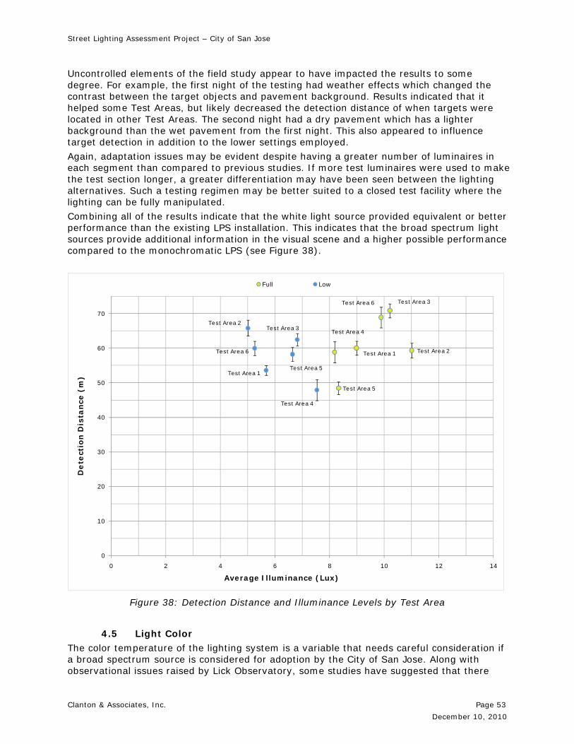
Street Lighting Assessment Project – City of San Jose
Clanton & Associates, Inc. Page 53
December 10, 2010
Uncontrolled elements of the field study appear to have impacted the results to some degree. For example, the first night of the testing had weather effects which changed the contrast between the target objects and pavement background. Results indicated that it helped some Test Areas, but likely decreased the detection distance of when targets were located in other Test Areas. The second night had a dry pavement which has a lighter background than the wet pavement from the first night. This also appeared to influence target detection in addition to the lower settings employed.
Again, adaptation issues may be evident despite having a greater number of luminaires in each segment than compared to previous studies. If more test luminaires were used to make the test section longer, a greater differentiation may have been seen between the lighting alternatives. Such a testing regimen may be better suited to a closed test facility where the lighting can be fully manipulated.
Combining all of the results indicate that the white light source provided equivalent or better performance than the existing LPS installation. This indicates that the broad spectrum light sources provide additional information in the visual scene and a higher possible performance compared to the monochromatic LPS (see Figure 38).
0
10
20
30
40
50
60
70
0 2 4 6 8 10 12 14
De
tect
ion
Dis
tance
(m
)
Average Illuminance (Lux)
Full Low
Test Area 1
Test Area 3Test Area 6
Test Area 2
Test Area 5
Test Area 3
Test Area 1Test Area 6
Test Area 4
Test Area 5
Test Area 4
Test Area 2
Figure 38: Detection Distance and Illuminance Levels by Test Area
4.5 Light Color
The color temperature of the lighting system is a variable that needs careful consideration if a broad spectrum source is considered for adoption by the City of San Jose. Along with observational issues raised by Lick Observatory, some studies have suggested that there

Street Lighting Assessment Project – City of San Jose
Clanton & Associates, Inc. Page 54
December 10, 2010
may be human and animal health risks from exposure to certain blue wavelengths of light, at certain intensities and durations. But the literature indicates that the issue is complex, poorly understood, and in need of much more research to understand cause and affect relationships. At present, it is not clear that outdoor lighting at typical exposures is likely to pose a threat to human health.
It is possible to use white light sources that emit lower levels of the wavelengths that may be of concern; however, the more that the blue wavelengths are reduced, the lower the energy efficiency of the source. The City will factor these issues into its decision-making and will monitor future research on this question.
There is more to the spectrum than the simple CCT value of the light source, as the frequency distribution of the light is an important aspect of this as well. While the CRI does provide some insight into this aspect of the light output, it is not a complete picture of the distribution as well. Spectral distribution graphs of the light source output are the best way to begin to fully appreciate the light sources.
4.6 Night Sky Considerations
The City of San Jose has a history of research and educational astronomy in nearby Lick Observatory. This is an important neighbor to the community and all sources of terrestrial lighting in the vicinity cause degradation to the observatory’s ability to do functional research at night.
The existing LPS light sources have several characteristics that are of particular benefit to the astronomy community. The first is the relatively long wavelength of the majority of the light (primary emission peak is at 589nm) is somewhat away from the offending short wavelengths.
Also, the source is essentially monochromatic, producing very little light at wavelengths other than the peak spike at 589nm. This means the astronomy community can filter their sensors at that specific wavelength with a sharp cutoff filter, and eliminate that portion of the spectrum very effectively without impacting other very useful wavelengths.
Broad spectrum technologies are a source of considerable concern for the astronomy community because they are now becoming efficient enough to compete with traditional sources for lumen efficiency. There is a broad movement to begin replacing the older technology with longer-life broad spectrum sources like LED and IND sources.
There are several emission frequency thresholds of particular concern for the astronomy community related to the broad spectrum sources. Wavelength emissions shorter than 550nm is of particular concern for Lick Observatory. Many LED light sources are built around a primary emission in the 440-460nm range, with phosphors to convert that to longer wavelengths. That strong emission peak is in a particularly damaging range for astronomy purposes.
The full array of the impacts of lighting is outside the scope of this report, but there is energy, environmental, and astronomical considerations that they City may want to consider in any decision-making process. Several of them are listed below.
1. Reduce the amount of light at night where possible. This is based on the ecologically-sound principle that there is an appropriate amount of light for a specific task, and more light does not equate to better lighting. In fact, in many cases, more light results in reduced visibility due to glare and other factors associated with the application of high-lumen light sources.
2. Reduce the amount of improperly applied light. This addresses light sources that are ineffectively applying light to a task, resulting in a considerable amount of wasted light in many situations. Improperly aimed floodlights produce a considerable amount

Street Lighting Assessment Project – City of San Jose
Clanton & Associates, Inc. Page 55
December 10, 2010
of skyglow, for example, especially compared to the percentage of light that they typically put on the actual task area.
3. Eliminate light pollution sources wherever possible. Many lights emit a small amount of uplight at low angles, even when adequately lighting the task in an otherwise suitable manner. This happens to be a critical condition for light pollution, and careful selection of luminaires with better performance in these critical conditions can result in a considerable improvement in the overall impact a luminaire produces.
4. Improve the quality of the light. Implement broad spectrum sources which provide increased visibility under lower light levels.
5. Control the spectral distribution of the light. This is important for astronomy research, and is in some ways in conflict with general lighting needs or benefits. The astronomy community is heavily impacted by short wavelength (blue end of the spectrum) light. This in one reason why the City of San Jose has used LPS to light the majority of the City for the last 30 years. Strategies that the City is considering, which are supported by this study, such as using directional LED lights, using lower wattage fixtures to replace the existing LPS luminaires, and dimming the lights in the late evening hours are ways to lessen the impacts to Lick Observatory.
0
0.1
0.2
0.3
0.4
0.5
0.6
0.7
0.8
0.9
1
380 430 480 530 580 630 680 730 780
Re
lati
ve S
pe
ctra
l P
ow
er
Wavelength (nm)
Test Area 4 LPS Test Area 2 HPS Test Area 1 IND
Figure 39: Spectral Power Distribution Curves Comparing LPS, HPS and IND.
(310 nm – 550nm)
Range of Special Concern for Lick Observatory
613 nm 590 nm
598 nm
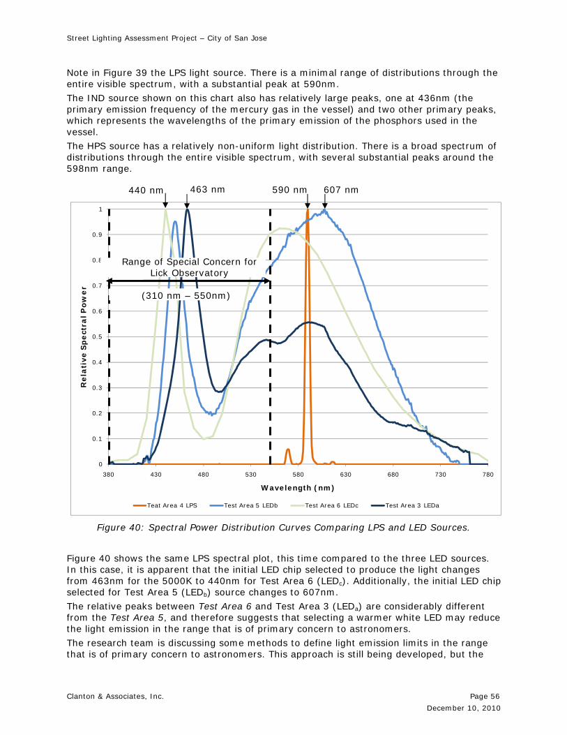
Street Lighting Assessment Project – City of San Jose
Clanton & Associates, Inc. Page 56
December 10, 2010
Note in Figure 39 the LPS light source. There is a minimal range of distributions through the entire visible spectrum, with a substantial peak at 590nm.
The IND source shown on this chart also has relatively large peaks, one at 436nm (the primary emission frequency of the mercury gas in the vessel) and two other primary peaks, which represents the wavelengths of the primary emission of the phosphors used in the vessel.
The HPS source has a relatively non-uniform light distribution. There is a broad spectrum of distributions through the entire visible spectrum, with several substantial peaks around the 598nm range.
0
0.1
0.2
0.3
0.4
0.5
0.6
0.7
0.8
0.9
1
380 430 480 530 580 630 680 730 780
Rela
tive
Sp
ect
ral P
ow
er
Wavelength (nm)
Teat Area 4 LPS Test Area 5 LEDb Test Area 6 LEDc Test Area 3 LEDa
Figure 40: Spectral Power Distribution Curves Comparing LPS and LED Sources.
Figure 40 shows the same LPS spectral plot, this time compared to the three LED sources. In this case, it is apparent that the initial LED chip selected to produce the light changes from 463nm for the 5000K to 440nm for Test Area 6 (LEDc). Additionally, the initial LED chip selected for Test Area 5 (LEDb) source changes to 607nm.
The relative peaks between Test Area 6 and Test Area 3 (LEDa) are considerably different from the Test Area 5, and therefore suggests that selecting a warmer white LED may reduce the light emission in the range that is of primary concern to astronomers.
The research team is discussing some methods to define light emission limits in the range that is of primary concern to astronomers. This approach is still being developed, but the
463 nm 590 nm 607 nm 440 nm
Range of Special Concern for Lick Observatory
(310 nm – 550nm)

Street Lighting Assessment Project – City of San Jose
Clanton & Associates, Inc. Page 57
December 10, 2010
basic premise behind the approach is to set percentage light output limits for the light source within certain ranges. There may be two different limits, one for a range of shorter wavelengths (possibly from 310nm to 450nm), and one for the longer range (from 450nm to 550nm). There could then be percentage output limits set based on proximity ranges to the observatory, so the regions closer have stricter percentage limits for the two emission ranges. Table 17 below shows the percent of emissions less than or equal to 500nm for each of the Test Areas.
Test Area Technology % Emissions <= 550nm
1 IND 46%
2 HPS 7%
3 LEDa 47%
4 LPS 0%
5 LEDb 34%
6 LEDc 39%
Table 17: Percent of Emissions Shorter than 550nm within visible spectrum (380-760nm)
The graph below identifies many of the light sources responsible for the various peaks as measured in the Lick skyglow observation data. This includes both terrestrial sources as well as naturally-occurring (airglow) sources.
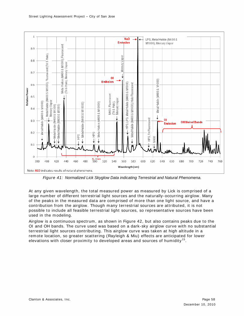
Street Lighting Assessment Project – City of San Jose
Clanton & Associates, Inc. Page 58
December 10, 2010
Figure 41: Normalized Lick Skyglow Data indicating Terrestrial and Natural Phenomena.
At any given wavelength, the total measured power as measured by Lick is comprised of a large number of different terrestrial light sources and the naturally-occurring airglow. Many of the peaks in the measured data are comprised of more than one light source, and have a contribution from the airglow. Though many terrestrial sources are attributed, it is not possible to include all feasible terrestrial light sources, so representative sources have been used in the modeling.
Airglow is a continuous spectrum, as shown in Figure 42, but also contains peaks due to the OI and OH bands. The curve used was based on a dark-sky airglow curve with no substantial terrestrial light sources contributing. This airglow curve was taken at high altitude in a remote location, so greater scattering (Rayleigh & Miu) effects are anticipated for lower elevations with closer proximity to developed areas and sources of humidity15.

Street Lighting Assessment Project – City of San Jose
Clanton & Associates, Inc. Page 59
December 10, 2010
Figure 42: Background Airglow Power Distribution
Figure 43 is a comparison of the Lick skyglow measurements and the estimated profile of atmospheric power due to terrestrial and naturally-occurring light sources. Both the terrestrial and naturally-occurring light sources were filtered through a model of Rayleigh scattering to account for reflections within the atmosphere.
Figure 43: Estimated Composite Profile and Lick Data Profile

Street Lighting Assessment Project – City of San Jose
Clanton & Associates, Inc. Page 60
December 10, 2010
Source Type Estimated Quantity
HPS 2%
MH400 19%
MH1000 19%
LPS 46%
Incandescent / Halogen 1%
4200K Halo Fluorescent 3%
4000K Tri Fluorescent 3%
cury Vapor 7%
Table 18: Estimated Percent of Skyglow Power Attributed to Each Terrestrial Light Source
As shown in Table 18, it is estimated that the LPS sources contribute most significantly to the measured skyglow, which is as anticipated due to the preponderance of LPS sources as street lighting. For each light source, a presumed distribution (percentage of uplight, light reflected from road and light reflected from grass) was established to develop the contribution of each light source to the total skyglow calculation.
Figure 44 shows the composite skyglow profile determined previously as compared to a skyglow profile where LPS sources have been eliminated and replaced with LED sources. Due to greater visibility efficiency, improved roadway task efficiency and the elimination of the direct uplight component through the specification of full-cutoff luminaires, the replacement of LPS sources with LED sources is not an even exchange of lighting power. Instead, the LED power used to replace the LPS power is approximately 33% lower in magnitude. This reduction is a terrestrial reduction, and does not include atmospheric effects.

Street Lighting Assessment Project – City of San Jose
Clanton & Associates, Inc. Page 61
December 10, 2010
Figure 44: Estimated Effect of Replacing LPS Sources with Reduced-Wattage LED Sources
Figure 45: Estimated Change in Relative Power of Sky Glow when LED sources are used to replace LPS sources
Figure 45 above demonstrates the anticipated change in skyglow power after LED sources have been used to replace LPS sources, where a positive number represents an increase in the lighting power at that wavelength and a negative number represents a decrease in the lighting power.
The strong negative spikes represent the substantial decreases in the skyglow spectrum directly associated with the removal of the fairly non-continuous LPS spectral distribution. The much less significant increases represent the contribution of a much more broad-spectrum light source (4000K LED) to the overall visible spectrum.
It is anticipated that the total benefit of the LED exchange will be an approximately 6.8% reduction in skyglow power experienced as skyglow, when accounting for atmospheric interaction without modifying the profile of other terrestrial sources. The skyglow reduction is increased to 13.6% when the lighting system is dimmed back to 50% light output at low traffic volume conditions.
4.7 Equivalent Driving Visibility
The difference between ‘roadway’ lighting and ‘street’ lighting is becoming more important to consider, as the current belief is that they require different visual tasks to perform adequately. Roadway lighting is provided for freeways where pedestrians and cyclists are not typically present. Street lighting is provided for major, collector and local roads where pedestrians and cyclists are generally present. The current IESNA recommendations were established when the de facto standard for street lighting and roadway lighting was HPS technology, so the performance conditions of emerging broad spectrum street lighting is not considered currently.

Street Lighting Assessment Project – City of San Jose
Clanton & Associates, Inc. Page 62
December 10, 2010
The City of San Jose’s use of IESNA 1964 as their Street Lighting Guidelines is currently under review and this variable should be considered in addition to that document to establish appropriate calculation procedures for broad spectrum sources.
4.8 Adaptive Standards Opportunities
Adaptive Street Lighting Control recognizes that exterior lighting criteria typically provides for the worst set of conditions that may exist for a given application. These conditions include traffic volume, the presence of pedestrians, ambient luminance, etc. Advances in lighting control technology allow for changes in luminaire light output that can potentially match the environmental (including traffic) conditions present at a particular time. The result not only reduces energy consumption of the street lighting system, but also prevents overlighting, reduces glare, and minimizes light pollution. RP-8-0516 describes all of the pedestrian conflict levels and implies the use of adaptive standards. The International Commission on Illumination (CIE 115:2010)17 also accounts for adaptive standards.
Regardless of the actual method of implementation, this study tested the concept of adaptive lighting. By lowering the light levels on the second night of the study, the team evaluated changes in visibility and subjective preference. It is important to note that none of the survey participants were aware of the light level they were viewing or even that dimming was part of the demonstration until after the survey.
The adoption of adaptive standards could provide criteria for a worst case, design level. The worst case may vary by roadway or street type but would be times of high traffic and pedestrian volume. A setback light level could then be assigned for times of much lower activity.
4.9 Limitations of the Project
The results of this project are inevitably affected by several factors that could not be addressed nor controlled given the constraints of the experiment. It cannot be overstated that locations for all of the luminaires were fixed and designed for the existing condition – a 135W LPS luminaire. In other words, the spacing and mounting height for all of the alternate systems were not optimized for the particular test luminaire, but rather installed in place of the existing LPS luminaire. The luminaires were placed in accordance with the existing spaced LPS pole locations.
The weather was a variable that could not be controlled throughout the evaluation. The varying degrees of surface brightness from the rain between the two evenings of evaluation contributed to the contrast reversal that was experienced and resulted in higher detection distances for two Test Areas (2 and 5) under lower light levels.
The mechanism in which the luminaires were adjusted between full and low settings was also a limitation. Since not all luminaire manufacturers were equipped with full dimming capabilities, some luminaires were adjusted to a low setting by reducing the output with the application of theater gel. Since not all luminaires were reduced by the same metric (power or light output) and by the same percentage, power and energy usages, in some cases, were predicted.
The demonstration and results apply for this particular type of roadway tested within the city limits of San Jose: a roadway through an industrial / office park. The results of this study do not necessarily apply directly to other zones such as residential and downtown areas. It is expected based upon these findings that subjectively participants would favor broad spectrum sources in other roadway types.

Street Lighting Assessment Project – City of San Jose
Clanton & Associates, Inc. Page 63
December 10, 2010
5.0 Conclusions
While it is important for the City to reduce overall energy consumption to meet the City’s Green Vision, it is also valuable to improve visual quality and preserve the night sky due to the close proximity to Lick Observatory. Given the site conditions (weather, color temperature, and control system), the assessment found favorable results (subjective and objective) for broad spectrum technologies utilizing light emitting diode (LED) and induction (IND) sources. These results add to the growing research on how the human eye perceives white light.
This assessment illustrates that advanced street light technologies that use broad spectrum light sources such as LED and IND can offer power savings of up to 40% without compromising the lighting design characteristics recommended for street lights. Combined with the power savings by using a lower wattage, more efficient broad spectrum technology, the energy savings experienced can be up to 60% if lighting levels are dimmed during periods of low activity through adaptive street lighting controls.
The subjective portion of the assessment indicates that San Jose residents prefer broad spectrum street lights. This suggests that the community will accept a change from the existing LPS to a white light source. Additionally, with the lights at a dimmed state on the second night of the assessment, participants did not feel that the Test Areas using broad spectrum technologies required additional light.
The objective performance portion of the assessment indicates that at full settings, detection distances utilizing broad spectrum technologies are on par or exceed those of traditional sources. It can also be noted that detection distances under broad spectrum light sources are not substantially affected by reduced light levels (low setting). Because detection distances under broad spectrum technologies were not substantially lower than the traditional sources under lower light conditions, the use of adaptive standards during periods of low activity is a viable option for the City.
In the evaluation of the Spectral Power Diagrams (SPD) for each of the broad spectrum technologies, there are wavelengths present within the range of special concern for Lick Observatory (310nm to 550nm). The presence of these wavelengths is difficult for observatories to filter out because there are multiple and broad peaks at varying wavelengths. The LPS works well for observatories because there is only one significant peak at a very narrow range of wavelengths. This makes it possible for the observatories to filter out the undesired wavelengths rather easily.
Installing lower wattage broad spectrum technology sources will reduce the overall light, but will add undesirable wavelengths for the observatory. Overall, it is anticipated that a complete change of LPS sources for LED sources could result in a 6.8% reduction in total terrestrial lighting power experienced as skyglow. This reduction can be increased to 13.6% when the lighting system applies an adaptive approach and is reduced to 50% light output.
Implementing adaptive street lighting controls, which will reduce the light level during periods of low activity, may be beneficial for the observatory by creating the greater benefit of much lower total light, regardless of the emitted wavelengths. In addition, using a broad spectrum technology in which the optics control the light in a downward manner more effectively may also minimize the adverse effect on the observatory.
The subjective survey and performance test results provide a starting point to consider a reinterpretation of traditional street lighting approaches based on new lighting technologies and better understanding of the visual performance of these various systems.

Street Lighting Assessment Project – City of San Jose
Clanton & Associates, Inc. Page 64
December 10, 2010
The Illuminating Engineering Society of North America (IESNA) has established a Mesopic Light Committee to recommend changes to the IESNA’s design guideline which takes into the consideration of broad spectrum technologies and the implications for street lighting. This study and others like it will inform the development of those guidelines. But the IESNA process is a lengthy one. Cities such as San Jose may wish to utilize design guidelines issued by the International Commission on Illumination (CIE) on mesopic lighting and adaptive lighting until such time as the IESNA revises its guidelines.
In summary, the findings of this study reinforce and augment those of other lighting researchers and the CIE which have found that broad spectrum sources can reduce energy consumption, improve nighttime vision, and improve the quality of the lighting on city streets. Using adaptive lighting can further reduce energy consumption and light pollution as can the use of directional lights, such as LEDs. The information found through the completion of this assessment can aid in the City’s quest to develop a Masterplan that utilizes broad spectrum technology and adaptive lighting control standards.

Street Lighting Assessment Project – City of San Jose
Clanton & Associates, Inc. Page 65
December 10, 2010
6.0 Appendix A: Subjective Lighting Survey Form
The subjective survey that was used for this assessment was developed by Peter Boyce while at the Lighting Research Center originally for the use of evaluating security lighting. The survey was then adapted by Boyce specifically for the use of exterior street lighting.
San Jose Nighttime Commercial Street Lighting Subjective Evaluation First Name Surveyor # Last Name
Thank you for participating in this important research on behalf of the City of San Jose! We are trying to understand the effect of different lighting systems for potential application throughout the City. The main goal is to understand public acceptance of various street lighting systems. Please respond to each of the questions with that goal in mind.
General Questions
G1. Do you live in San Jose?
Yes ________ No__________
G2. Do you live within two blocks of the Hellyer Avenue test area?
Yes ________ No__________
G3. Do you work in the lighting industry? (design, manufacturer, specification, sales)
Yes ________ No__________
Demographic Questions
D1 Gender M F (circle one)
D2 Age (in years)
D3 Zip Code

Street Lighting Assessment Project – City of San Jose
Clanton & Associates, Inc. Page 66
December 10, 2010
Nighttime San Jose Street Lighting Subjective Evaluation Surveyor #
S1. Weather conditions --- Clear _____ Cloudy_____ Rain_____ Fog_____
S2. Ground conditions --- Streets Dry _____ Streets Wet_____
All of the statements in the table below (except #1) refer to the lighting of the immediate area around you, during darkness. Please rate your level of agreement with each of the following statements about the lighting, on a 1 to 5 scale, with 1 being ‘strongly disagree’ and 5 being ‘strongly agree’.
Rate Statements Strongly Disagree ……..…Neutral..…..…...Strongly Don’t Know 1 It would be safe to walk here, alone, during daylight hours. 1 2 3 4 5 DK
2 It would be safe to walk here, alone, during darkness hours. 1 2 3 4 5 DK
3 The lighting is comfortable. 1 2 3 4 5 DK
4 There is too much light on the street. 1 2 3 4 5 DK
5 There is not enough light on the street. 1 2 3 4 5 DK
6 The light is uneven (patchy). 1 2 3 4 5 DK
7 The light sources are glaring. 1 2 3 4 5 DK
8 It would be safe to walk on the sidewalk here at night. 1 2 3 4 5 DK
9 I cannot tell the colors of things due to the lighting. 1 2 3 4 5 DK
10 The lighting enables safe vehicular navigation. 1 2 3 4 5 DK
11 I like the color of the light. 1 2 3 4 5 DK
12 I would like this style lighting on my city streets. 1 2 3 4 5 DK
13. How does the lighting in this area compare with the lighting of similar San Jose city streets at night?
Much worse Worse About the same Better Much Better
14. Write additional comments below.

Street Lighting Assessment Project – City of San Jose
Clanton & Associates, Inc. Page 67
December 10, 2010
7.0 Appendix B: Subjective Survey Participant Comments
Test Area 1 In general, the comments for Test Area 1 show that participants liked the lighting. It was commented on from several participants that the distribution was ‘patchy’. Surveyor Number
Comment
6 As much as I support the environment, I wonder if it is wise to spend money changing lights when we are laying off police and firefighters.
8 Colors of grass and trees very true 10 I have walked this street before during the day 12 Like how light spreads 13 Good lights 16 Dark patches between lights. Headlights on test vehicle skewing results 18 The light does not overlap 19 Full cutoff fixtures – good, less glare, more efficient, would be less patchy if the
poles were closer together but for me these are perfectly okay as is. 24 Question: Why does it matter if someone from outside a residential
neighborhood feels “safe” there. 1: Not objective or subjective – Imaginary (it’s night). 2: Not objective or subjective (we’re not alone).
27 The lights are quiet, very little buzzing. I like how these lights simulate daylight colors. Lighting is uneven though.
28 The lighting is patchy and there is a big dark open field at night 37 I prefer short lights because they are less affect by trees and they don’t shine
into our houses. Too white! White light is not natural 38 This is the best light for pedestrians. Patchy uneven light due to distance
between lights. I like the white color of light. I like this light. 39 The side fencing gives a sense of safety 44 Lighting not evenly distributed 48 I don’t like it, but in my ‘hood – safer! 50 Very well lit, no glare nor patchiness. Very nice! Note: I liked the best! 52 Spotlight 53 No more yellow! 57 I really like this type of light! (better than # 4, 6, and 5). The softer color is
nice! 60 Good but very patchy 63 I like the improvement 65 I like what I see 66 I love these lights
NIGHT 2
109 Trees cause dark spots 110 I could not see the sidewalk cracks in people’s shadows 111 Lights too dim! 140 Excellent at keeping light out of your eyes and down on the street 155 Good color, a little harsh directly 166 Overall liked it, #1 and #2 top choices. 169 Not enough light between poles 170 The breakaway curbs in ALL areas might cause some negative problems when
walking 178 This area in general is nicer than the rest of the areas. No buildings at all and
some very nice trees in the background. I wonder if this skews perception of

Street Lighting Assessment Project – City of San Jose
Clanton & Associates, Inc. Page 68
December 10, 2010
how good the lights look? 180 Easy to read under this light
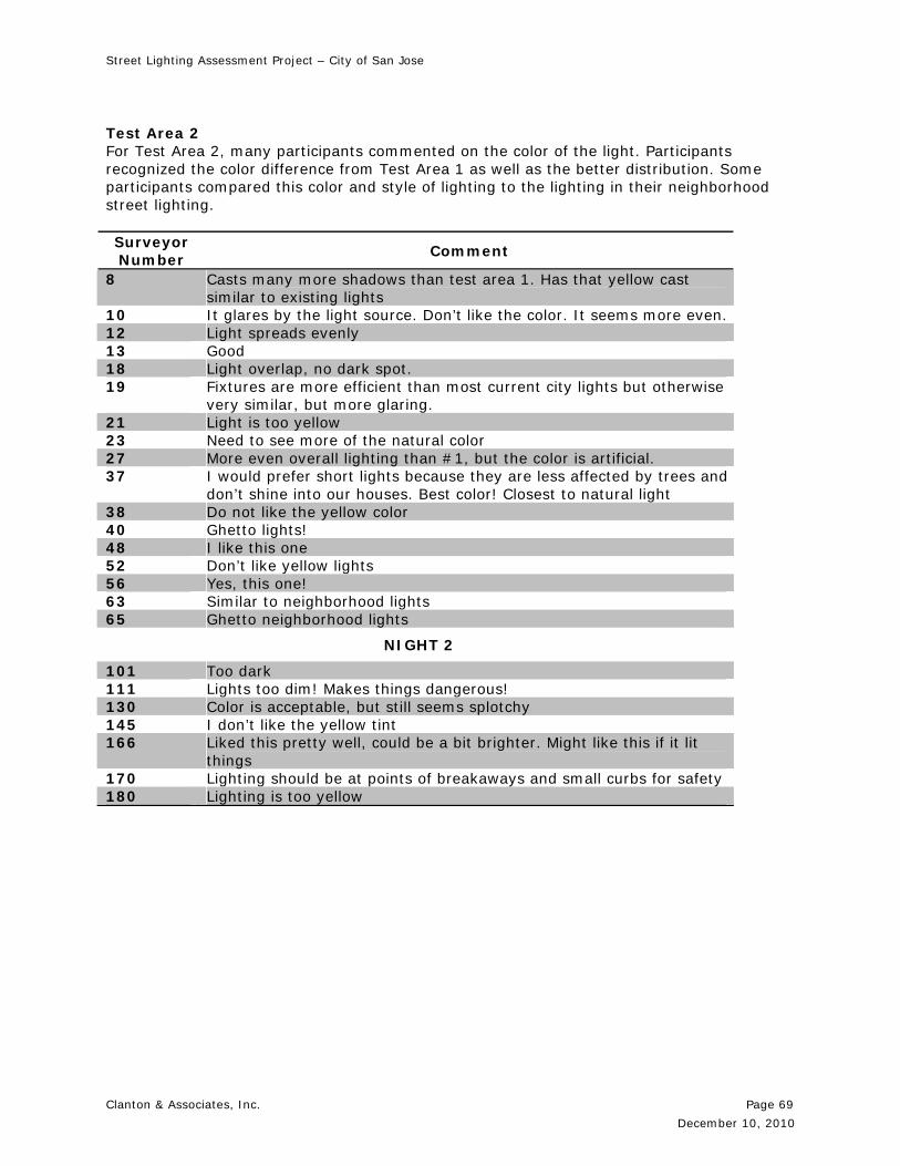
Street Lighting Assessment Project – City of San Jose
Clanton & Associates, Inc. Page 69
December 10, 2010
Test Area 2 For Test Area 2, many participants commented on the color of the light. Participants recognized the color difference from Test Area 1 as well as the better distribution. Some participants compared this color and style of lighting to the lighting in their neighborhood street lighting. Surveyor Number
Comment
8 Casts many more shadows than test area 1. Has that yellow cast similar to existing lights
10 It glares by the light source. Don’t like the color. It seems more even. 12 Light spreads evenly 13 Good 18 Light overlap, no dark spot. 19 Fixtures are more efficient than most current city lights but otherwise
very similar, but more glaring. 21 Light is too yellow 23 Need to see more of the natural color 27 More even overall lighting than #1, but the color is artificial. 37 I would prefer short lights because they are less affected by trees and
don’t shine into our houses. Best color! Closest to natural light 38 Do not like the yellow color 40 Ghetto lights! 48 I like this one 52 Don’t like yellow lights 56 Yes, this one! 63 Similar to neighborhood lights 65 Ghetto neighborhood lights
NIGHT 2
101 Too dark 111 Lights too dim! Makes things dangerous! 130 Color is acceptable, but still seems splotchy 145 I don’t like the yellow tint 166 Liked this pretty well, could be a bit brighter. Might like this if it lit
things 170 Lighting should be at points of breakaways and small curbs for safety 180 Lighting is too yellow

Street Lighting Assessment Project – City of San Jose
Clanton & Associates, Inc. Page 70
December 10, 2010
Test Area 3 In comparison to the previous Test Areas, participants generally like this type of lighting better, although there are several comments on the color of the light being too blue/grey. The comments from the second night are generally the same. Some participants commented that the lights were too dim. Surveyor #
Comment
2 All too bright 6 Feels like an industrial park 8 More of a blue cast to the light. Light source casts more glare. 10 It looks very clear and sterile. I feel like in an office 12 Light does not spread 13 Good 18 Shadows are easily cast. Unable to read paper. 19 A little too much light shines off to the sides which contributes to
glare. 23 Excellent work 27 This was my favorite so far. I like no color which is daylight-like and it
is much more even and brighter than #1 35 When we first walked into these lights, they seemed very blue but
after standing here a while the color seems nice 37 I prefer short lights because they are less affect by trees and they
don’t shine into our houses. Too white! White light is not natural 38 More even than #1 but not as bright. Need brighter for pedestrians 40 Yeea 44 The lights are great if you are out walking. Maybe too bright if I were
driving a car or have one outside my bedroom window. 48 Best yet 50 Streets are well lit but a bit bright causing a slight glare 53 Anything is better than yellow 57 Too much glare, the white light is harsh! 58 This is the best one of all, softer yet enough light 62 This light is great, better than many others 63 Good lighting 67 It’s a winner
NIGHT 2
101 Too dim 103 Lights look broken 111 Lights look safe! 130 Although this luminaire seems to have more glare it produces a pretty
even illumination of the road and sidewalk 133 Greyness is weird, but light seems adequate on street but not on
sides 145 I like that the fixtures cover a larger area 155 Good spread, maybe too much light scatter? Keep focused down. 166 Unpleasant 169 Blech 170 Good colors for traffic light safety 172 Dark areas between lamp posts is much less than #1 and #2. Good
dispersion

Street Lighting Assessment Project – City of San Jose
Clanton & Associates, Inc. Page 71
December 10, 2010
174 Can’t read the form well here. Brighter, but less comfortable. 180 The lighting is dim and bluish Test Area 4 Many participants recognized the luminaires in this Test Area as the San Jose City Standard. Participants also commented on the yellow color of the light and difficultly of colors to be accurately rendered. Surveyor #
Comment
3 Standard St Lighting 6 These lights are so bright, I cant tell if my headlights are on 8 The unmistakable central lights! Boy, they cast a lot of shadows! 10 This is the lighting I am used to 19 Too much light shines off to the sides – increases glare and wastes
light 23 Don’t really like 27 I really don’t like the color of these lights 37 I prefer short lights because they are less affect by trees and they
don’t shine into our houses. Too yellow. Unpleasant. 38 I don’t like yellow light 40 Nope 52 Nauseating light 53 All lighting in San Jose is difficult and unsafe 57 Way too much glare! Not enough light intensity directed towards the
ground 63 Too old fashioned 67 Old lights 73 Give more time to write
NIGHT 2
101 Poor color, but bright. 107 Our lights are weaker 111 I will still feel unsafe in my neighborhood with these lights! 133 Glare from fixture/lamp interferes with light quality. 152 Current San Jose, but brighter 154 I like the color 155 Bad, awful glare, impedes direct view of stars 166 Ugly light 170 Amber lighting is not too safe – blends into the yellow in the traffic
signal 172 Good brightness – but loss of color detail is annoying. Landscaping not
interesting under this color of light 174 Glary and too dim 179 Looks exactly like my street
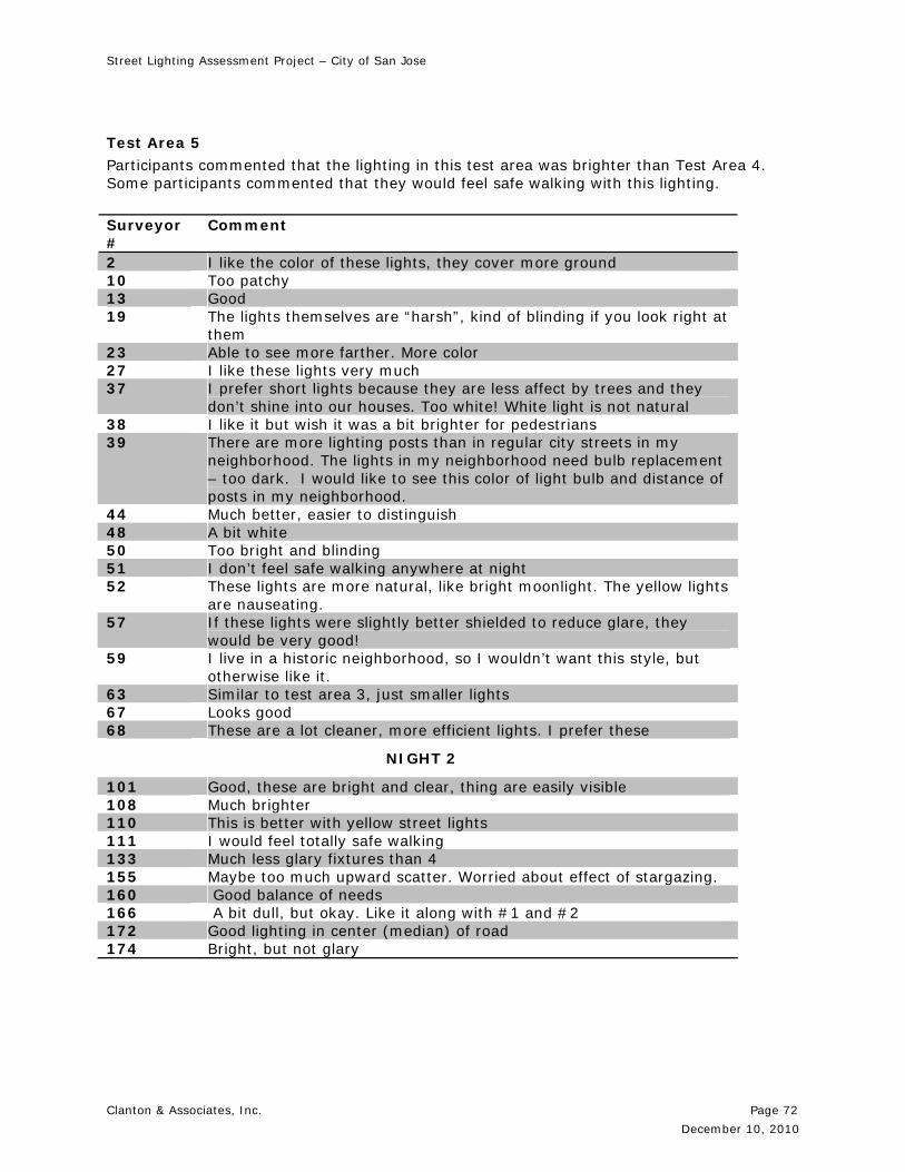
Street Lighting Assessment Project – City of San Jose
Clanton & Associates, Inc. Page 72
December 10, 2010
Test Area 5 Participants commented that the lighting in this test area was brighter than Test Area 4. Some participants commented that they would feel safe walking with this lighting.
Surveyor #
Comment
2 I like the color of these lights, they cover more ground 10 Too patchy 13 Good 19 The lights themselves are “harsh”, kind of blinding if you look right at
them 23 Able to see more farther. More color 27 I like these lights very much 37 I prefer short lights because they are less affect by trees and they
don’t shine into our houses. Too white! White light is not natural 38 I like it but wish it was a bit brighter for pedestrians 39 There are more lighting posts than in regular city streets in my
neighborhood. The lights in my neighborhood need bulb replacement – too dark. I would like to see this color of light bulb and distance of posts in my neighborhood.
44 Much better, easier to distinguish 48 A bit white 50 Too bright and blinding 51 I don’t feel safe walking anywhere at night 52 These lights are more natural, like bright moonlight. The yellow lights
are nauseating. 57 If these lights were slightly better shielded to reduce glare, they
would be very good! 59 I live in a historic neighborhood, so I wouldn’t want this style, but
otherwise like it. 63 Similar to test area 3, just smaller lights 67 Looks good 68 These are a lot cleaner, more efficient lights. I prefer these
NIGHT 2
101 Good, these are bright and clear, thing are easily visible 108 Much brighter 110 This is better with yellow street lights 111 I would feel totally safe walking 133 Much less glary fixtures than 4 155 Maybe too much upward scatter. Worried about effect of stargazing. 160 Good balance of needs 166 A bit dull, but okay. Like it along with #1 and #2 172 Good lighting in center (median) of road 174 Bright, but not glary

Street Lighting Assessment Project – City of San Jose
Clanton & Associates, Inc. Page 73
December 10, 2010
Test Area 6 In general, many participants noticed the increase in color temperature of these lights compared to Test Area 5. Participants noticed and generally liked the lighting in Test Area 5 better.
Surveyor #
Comment
6 Feels like an industrial site. It would have been nice to have hot chocolate and cookies when we got back.
10 I like the color, but too patchy 13 Good 19 The lights themselves are a little harsh if you look right at them.
Maybe not quite as much as #5, but close. Slightly too much light going off to the sides, but not bad.
27 These are too dim and patchy. They might be ok late at night with little vehicle and foot traffic.
35 Seems possibly more blue than #5? Prefer less blue. 37 I prefer short lights because they are less affect by trees and they
don’t shine into our houses. Too white! White light is not natural 38 I like this light, is there anything between this and number 1? 39 More light posts on this road than my neighborhood. What about
bridges and tunnels? In here pedestrians use for daily traffic (e.g. bridge between bambi lane and dobem avenue (near capital park)). Not a lot of traffic to really assess. Sidewalks in much better state.
40 I like, I like. Smiley Face 44 These lights are a bit of a glare compared to the lights in test area 5. 50 Too glaring but less patchy from test #5 53 I liked #5 better that #6 but anything is better than yellow 57 Very slightly better than #5, slightly less glare, more comfortable. 63 Ok 67 It’s workable 74 It’s dim
NIGHT 2
101 Dim 111 I would prefer these lights in my neighborhood the best. 133 Still glary even though very dim by comparison to 4 or 5 147 Its really cold light 155 Glare, decent scatter shielding. Could help with star viewing 166 Too dull. Don’t like color. Felt like big fluorescent lights. 170 Can see traffic lights better in this lighting 172 Good lighting at center (median) of street. Patchy 174 Soft, not bad, but I would like brighter 178 I would like the City to strongly consider street trees when deciding
what type of lights and fixtures to use. I am advocate of trees.
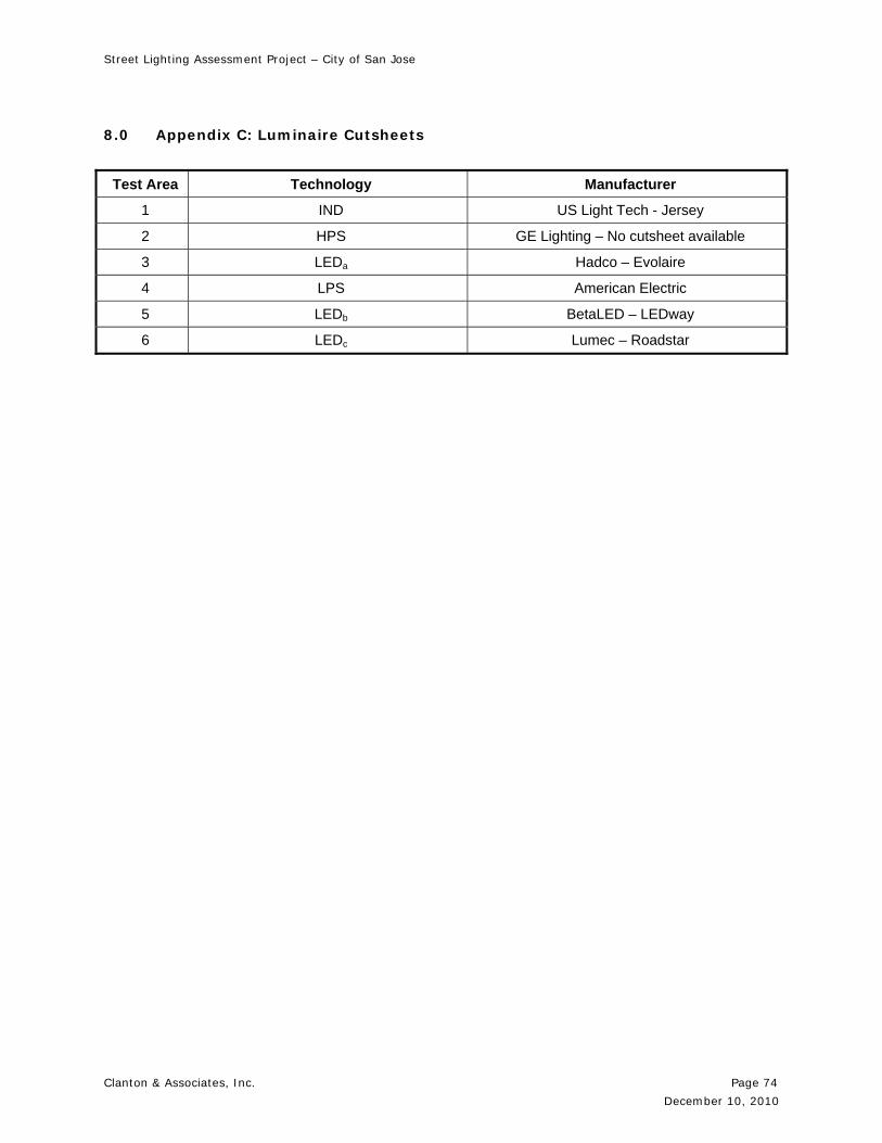
Street Lighting Assessment Project – City of San Jose
Clanton & Associates, Inc. Page 74
December 10, 2010
8.0 Appendix C: Luminaire Cutsheets
Test Area Technology Manufacturer
1 IND US Light Tech - Jersey
2 HPS GE Lighting – No cutsheet available
3 LEDa Hadco – Evolaire
4 LPS American Electric
5 LEDb BetaLED – LEDway
6 LEDc Lumec – Roadstar
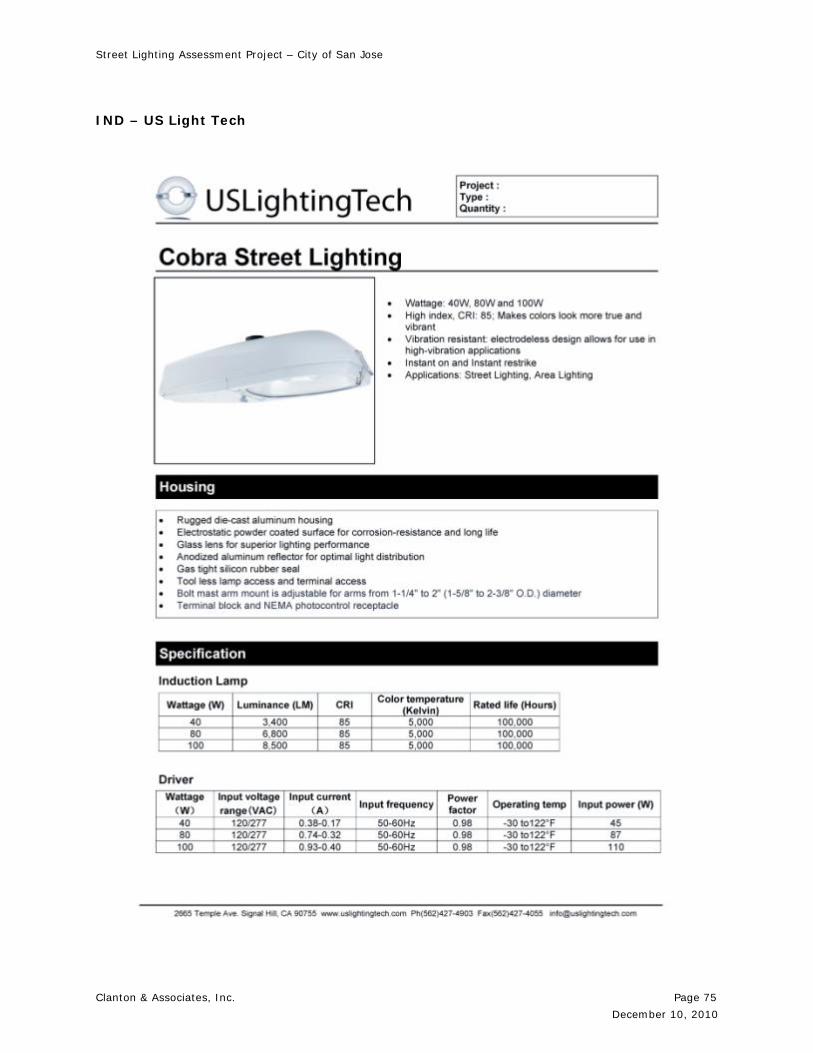
Street Lighting Assessment Project – City of San Jose
Clanton & Associates, Inc. Page 75
December 10, 2010
IND – US Light Tech

Street Lighting Assessment Project – City of San Jose
Clanton & Associates, Inc. Page 76
December 10, 2010
HPS – GE Lighting No cutsheet available for this luminaire.

Street Lighting Assessment Project – City of San Jose
Clanton & Associates, Inc. Page 77
December 10, 2010
LEDa – Hadco

Street Lighting Assessment Project – City of San Jose
Clanton & Associates, Inc. Page 78
December 10, 2010
LPS- American Electric

Street Lighting Assessment Project – City of San Jose
Clanton & Associates, Inc. Page 79
December 10, 2010
LEDb- BetaLED
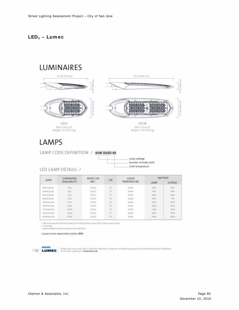
Street Lighting Assessment Project – City of San Jose
Clanton & Associates, Inc. Page 80
December 10, 2010
LEDc – Lumec

Street Lighting Assessment Project – City of San Jose
Clanton & Associates, Inc. Page 81
December 10, 2010

Street Lighting Assessment Project – City of San Jose
Clanton & Associates, Inc. Page 82
December 10, 2010
9.0 Appendix D: Relative Sky Glow Spectral Calculations
Following are energy output graphs of the six light sources (absolute output graphs, representing power per wavelength).
0
0.0001
0.0002
0.0003
0.0004
0.0005
0.0006
0.0007
0.0008
300 400 500 600 700 800
En
erg
y
Wavelength (nm)
Induction
Figure 46: SPD for Test Area 1

Street Lighting Assessment Project – City of San Jose
Clanton & Associates, Inc. Page 83
December 10, 2010
0.000
0.000
0.000
0.000
0.000
0.001
0.001
0.001
0.001
350 400 450 500 550 600 650 700 750 800
En
erg
y
Wavelength (nm)
Figure 47: SPD for Test Area 2
0
0.0001
0.0002
0.0003
0.0004
0.0005
0.0006
0.0007
0.0008
300 400 500 600 700 800
En
erg
y
Wavelength (nm)
Figure 48: SPD for Test Area 3
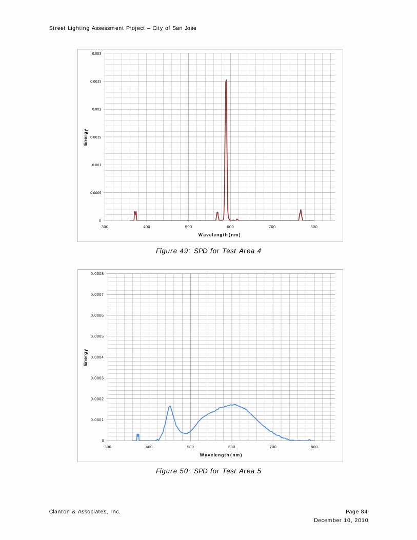
Street Lighting Assessment Project – City of San Jose
Clanton & Associates, Inc. Page 84
December 10, 2010
0
0.0005
0.001
0.0015
0.002
0.0025
0.003
300 400 500 600 700 800
En
erg
y
Wavelength (nm)
Figure 49: SPD for Test Area 4
0
0.0001
0.0002
0.0003
0.0004
0.0005
0.0006
0.0007
0.0008
300 400 500 600 700 800
En
erg
y
Wavelength (nm)
Figure 50: SPD for Test Area 5
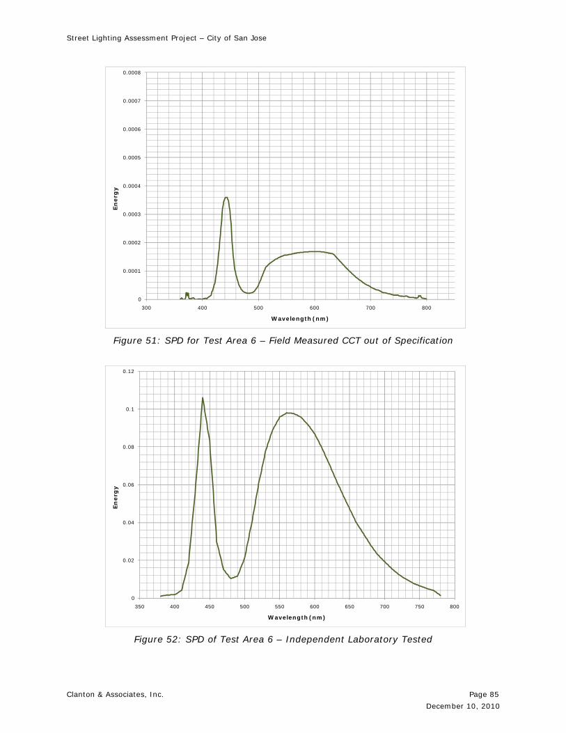
Street Lighting Assessment Project – City of San Jose
Clanton & Associates, Inc. Page 85
December 10, 2010
0
0.0001
0.0002
0.0003
0.0004
0.0005
0.0006
0.0007
0.0008
300 400 500 600 700 800
En
erg
y
Wavelength (nm)
Figure 51: SPD for Test Area 6 – Field Measured CCT out of Specification
0
0.02
0.04
0.06
0.08
0.1
0.12
350 400 450 500 550 600 650 700 750 800
En
erg
y
Wavelength (nm)
Figure 52: SPD of Test Area 6 – Independent Laboratory Tested
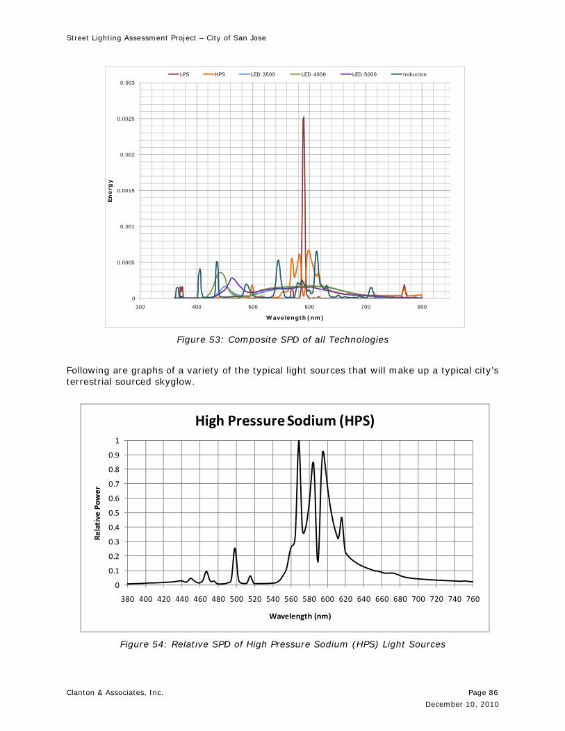
Street Lighting Assessment Project – City of San Jose
Clanton & Associates, Inc. Page 86
December 10, 2010
0
0.0005
0.001
0.0015
0.002
0.0025
0.003
300 400 500 600 700 800
En
erg
y
Wavelength (nm)
LPS HPS LED 3500 LED 4000 LED 5000 Induction
Figure 53: Composite SPD of all Technologies
Following are graphs of a variety of the typical light sources that will make up a typical city’s terrestrial sourced skyglow.
0
0.1
0.2
0.3
0.4
0.5
0.6
0.7
0.8
0.9
1
380 400 420 440 460 480 500 520 540 560 580 600 620 640 660 680 700 720 740 760
Relative
Power
Wavelength (nm)
High Pressure Sodium (HPS)
Figure 54: Relative SPD of High Pressure Sodium (HPS) Light Sources
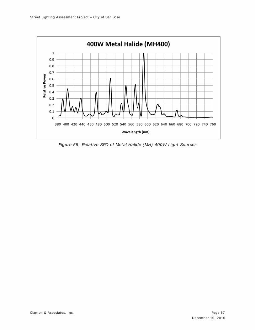
Street Lighting Assessment Project – City of San Jose
Clanton & Associates, Inc. Page 87
December 10, 2010
0
0.1
0.2
0.3
0.4
0.5
0.6
0.7
0.8
0.9
1
380 400 420 440 460 480 500 520 540 560 580 600 620 640 660 680 700 720 740 760
Relative
Power
Wavelength (nm)
400W Metal Halide (MH400)
Figure 55: Relative SPD of Metal Halide (MH) 400W Light Sources
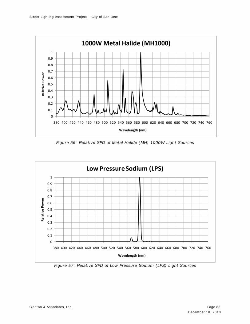
Street Lighting Assessment Project – City of San Jose
Clanton & Associates, Inc. Page 88
December 10, 2010
0
0.1
0.2
0.3
0.4
0.5
0.6
0.7
0.8
0.9
1
380 400 420 440 460 480 500 520 540 560 580 600 620 640 660 680 700 720 740 760
Relative
Power
Wavelength (nm)
1000W Metal Halide (MH1000)
Figure 56: Relative SPD of Metal Halide (MH) 1000W Light Sources
0
0.1
0.2
0.3
0.4
0.5
0.6
0.7
0.8
0.9
1
380 400 420 440 460 480 500 520 540 560 580 600 620 640 660 680 700 720 740 760
Relative
Power
Wavelength (nm)
Low Pressure Sodium (LPS)
Figure 57: Relative SPD of Low Pressure Sodium (LPS) Light Sources
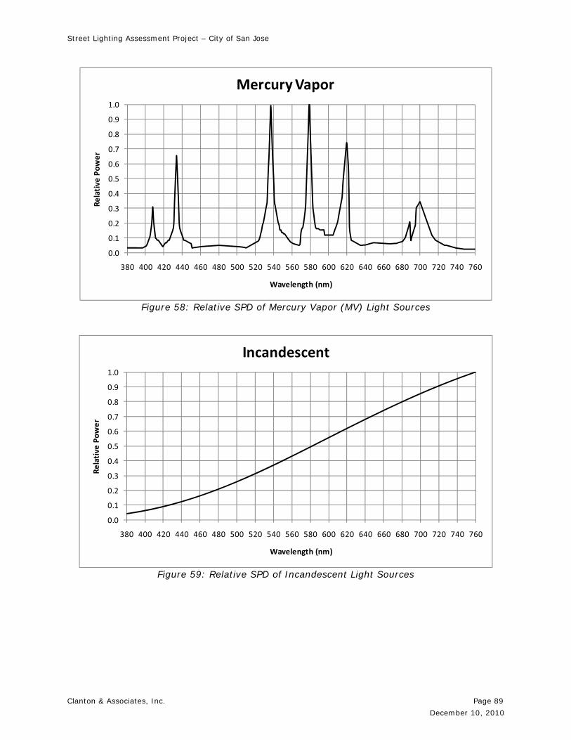
Street Lighting Assessment Project – City of San Jose
Clanton & Associates, Inc. Page 89
December 10, 2010
0.0
0.1
0.2
0.3
0.4
0.5
0.6
0.7
0.8
0.9
1.0
380 400 420 440 460 480 500 520 540 560 580 600 620 640 660 680 700 720 740 760
Relative
Power
Wavelength (nm)
Mercury Vapor
Figure 58: Relative SPD of Mercury Vapor (MV) Light Sources
0.0
0.1
0.2
0.3
0.4
0.5
0.6
0.7
0.8
0.9
1.0
380 400 420 440 460 480 500 520 540 560 580 600 620 640 660 680 700 720 740 760
Relative
Power
Wavelength (nm)
Incandescent
Figure 59: Relative SPD of Incandescent Light Sources

Street Lighting Assessment Project – City of San Jose
Clanton & Associates, Inc. Page 90
December 10, 2010
0.0
0.1
0.2
0.3
0.4
0.5
0.6
0.7
0.8
0.9
1.0
380 400 420 440 460 480 500 520 540 560 580 600 620 640 660 680 700 720 740 760
Relative
Power
Wavelength (nm)
Halogen
Figure 60: Relative SPD of Halogen Light Sources
0.0
0.1
0.2
0.3
0.4
0.5
0.6
0.7
0.8
0.9
1.0
380 400 420 440 460 480 500 520 540 560 580 600 620 640 660 680 700 720 740 760
Relative
Power
Wavelength (nm)
4200K Halophosphor Fluorescent
Figure 61: Relative SPD of 4200K Halophosphor (T12) Light Sources
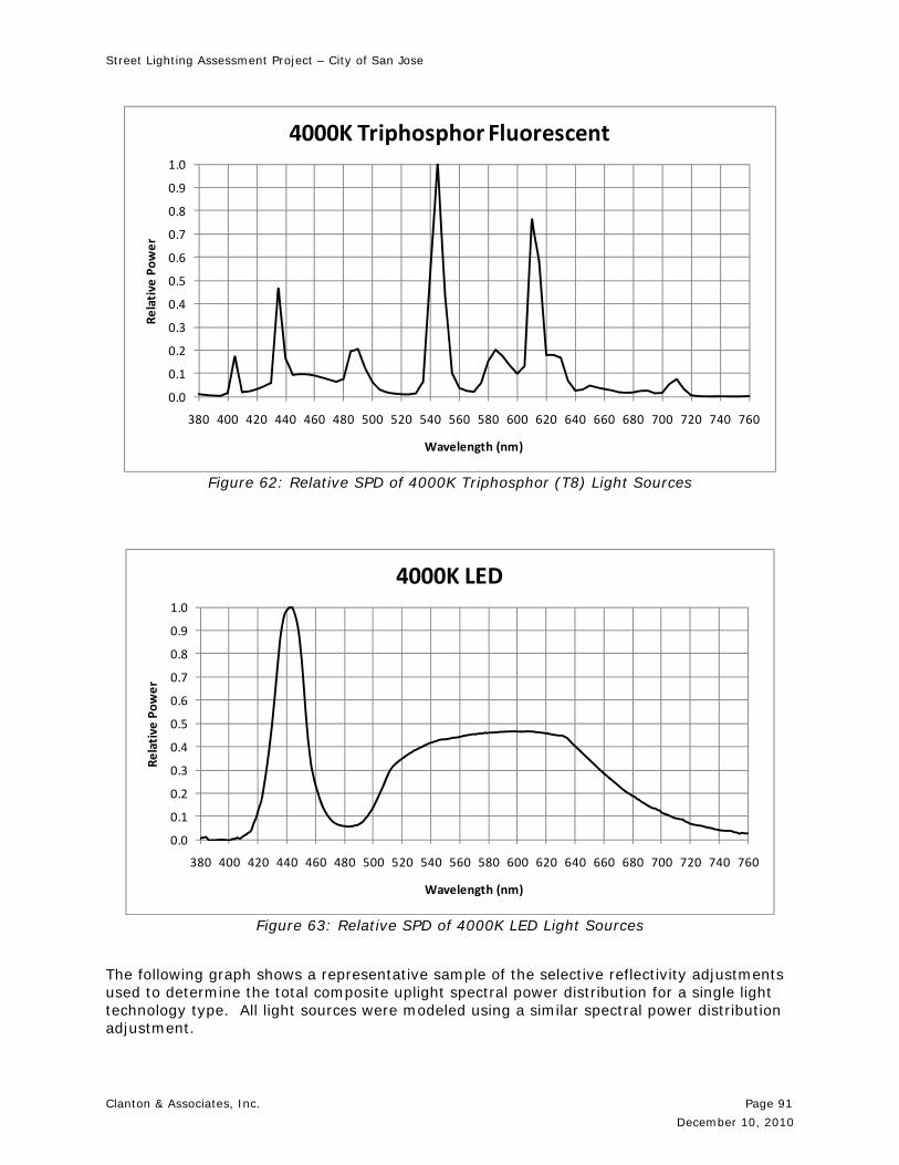
Street Lighting Assessment Project – City of San Jose
Clanton & Associates, Inc. Page 91
December 10, 2010
0.0
0.1
0.2
0.3
0.4
0.5
0.6
0.7
0.8
0.9
1.0
380 400 420 440 460 480 500 520 540 560 580 600 620 640 660 680 700 720 740 760
Relative
Power
Wavelength (nm)
4000K Triphosphor Fluorescent
Figure 62: Relative SPD of 4000K Triphosphor (T8) Light Sources
0.0
0.1
0.2
0.3
0.4
0.5
0.6
0.7
0.8
0.9
1.0
380 400 420 440 460 480 500 520 540 560 580 600 620 640 660 680 700 720 740 760
Relative
Power
Wavelength (nm)
4000K LED
Figure 63: Relative SPD of 4000K LED Light Sources
The following graph shows a representative sample of the selective reflectivity adjustments used to determine the total composite uplight spectral power distribution for a single light technology type. All light sources were modeled using a similar spectral power distribution adjustment.
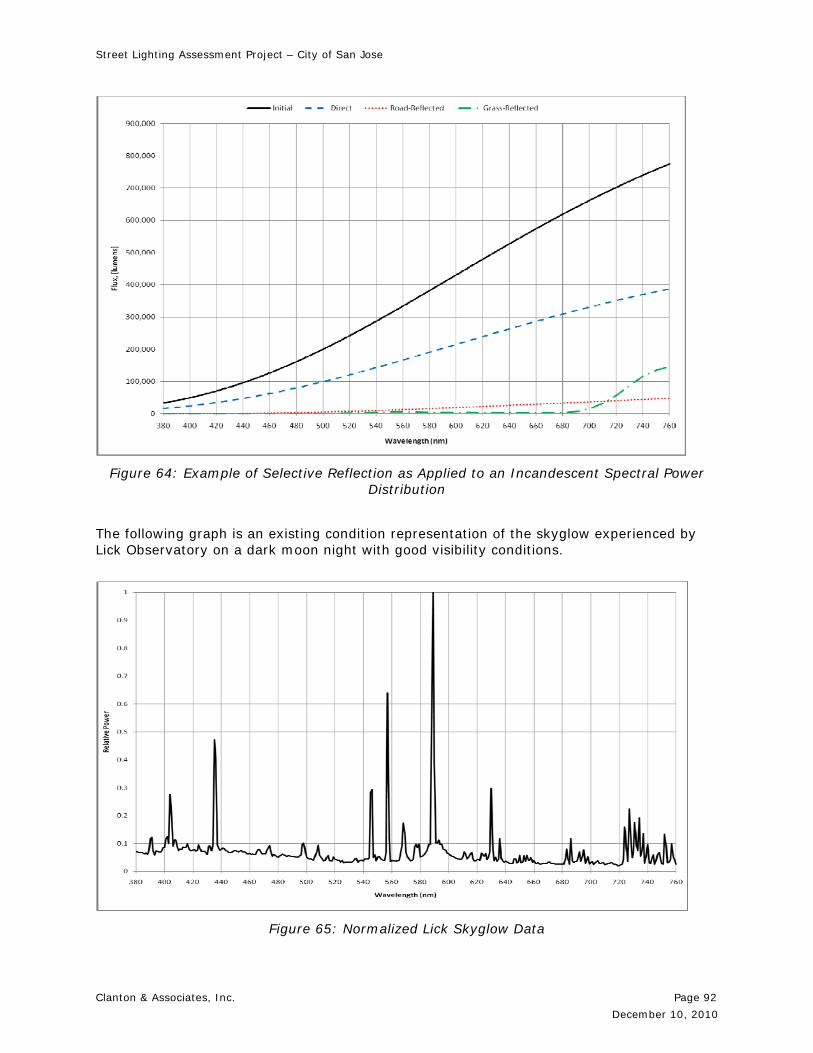
Street Lighting Assessment Project – City of San Jose
Clanton & Associates, Inc. Page 92
December 10, 2010
Figure 64: Example of Selective Reflection as Applied to an Incandescent Spectral Power Distribution
The following graph is an existing condition representation of the skyglow experienced by Lick Observatory on a dark moon night with good visibility conditions.
Figure 65: Normalized Lick Skyglow Data

Street Lighting Assessment Project – City of San Jose
Clanton & Associates, Inc. Page 93
December 10, 2010
The following graph provides annotation of a variety of the terrestrial and naturally-occurring (airglow) light sources that are represented in the existing condition Lick Observatory curve.
Figure
66
: Nor
mal
ized
Lic
k S
kygl
ow D
ata
indi
catin
g T
erre
stria
l and
Nat
ural
Phe
nom
ena

Street Lighting Assessment Project – City of San Jose
Clanton & Associates, Inc. Page 94
December 10, 2010
The following graph provides a representative curve for naturally-occurring light emissions (airglow) for a dark environment.
Figure 67: Background Airglow Power Distribution
The following graph is a comparison of the Lick skyglow measurements and the estimated profile of atmospheric power due to terrestrial and naturally-occurring light sources. Both the terrestrial and naturally-occurring light sources were filtered through a model of Rayleigh scattering to account for reflections within the atmosphere.
Figure 68: Estimated Composite Profile and Lick Data Profile

Street Lighting Assessment Project – City of San Jose
Clanton & Associates, Inc. Page 95
December 10, 2010
Source Type Estimated Quantity
HPS 1.9%
MH400 19.3%
MH1000 19.3%
LPS 45.7%
Incandescent 0.5%
Halogen 0.5%
4200K Halo Fluorescent 2.9%
4000K Tri Fluorescent 2.9%
Mercury Vapor 7.0%
Table 19: Estimated Percent of Skyglow Power Attributed to Each Terrestrial Light Source
As shown above, it is estimated that the LPS sources contribute most significantly to the measured skyglow, which is as anticipated due to the preponderance of LPS sources as street lighting. For each light source, a presumed distribution (percentage of uplight, light reflected from road and light reflected from grass) was established to develop the contribution of each light source to the total skyglow calculation.
The following graph shows the composite sky glow profile determined previously as compared to a sky glow profile where LPS sources have been eliminated and replaced with LED sources. Due to greater visibility efficiency, improved roadway task efficiency and the elimination of the direct uplight component through the specification of full-cutoff luminaires, the replacement of LPS sources with LED sources is not an even exchange of lighting power. Instead, the LED power used to replace the LPS power is approximately 33% lower in magnitude.
Figure 69: Estimated Effect of Replacing LPS Sources with Reduced-Wattage LED Sources

Street Lighting Assessment Project – City of San Jose
Clanton & Associates, Inc. Page 96
December 10, 2010
Figure 70: Estimated Change in Relative Power of Sky Glow when LED sources are used to replace LPS sources
The graph above demonstrates the anticipated change in skyglow power after LED sources have been used to replace LPS sources, where a positive number represents an increase in the lighting power at that wavelength and a negative number represents a decrease in the lighting power.
The strong negative spikes represent the substantial decreases in the skyglow spectrum directly associated with the removal of the fairly non-continuous LPS spectral distribution. The much less significant increases represent the contribution of a much more broad-spectrum light source (4000K LED) to the overall visible spectrum.

Street Lighting Assessment Project – City of San Jose
Clanton & Associates, Inc. Page 97
December 10, 2010
10.0 Appendix E: Site Calculations
Test Area 1
Figure 71: Illuminance Calculation for Test Area 1 (Typical Spacing)
Illuminance Scale (fc)
0 0.5 1 1.5
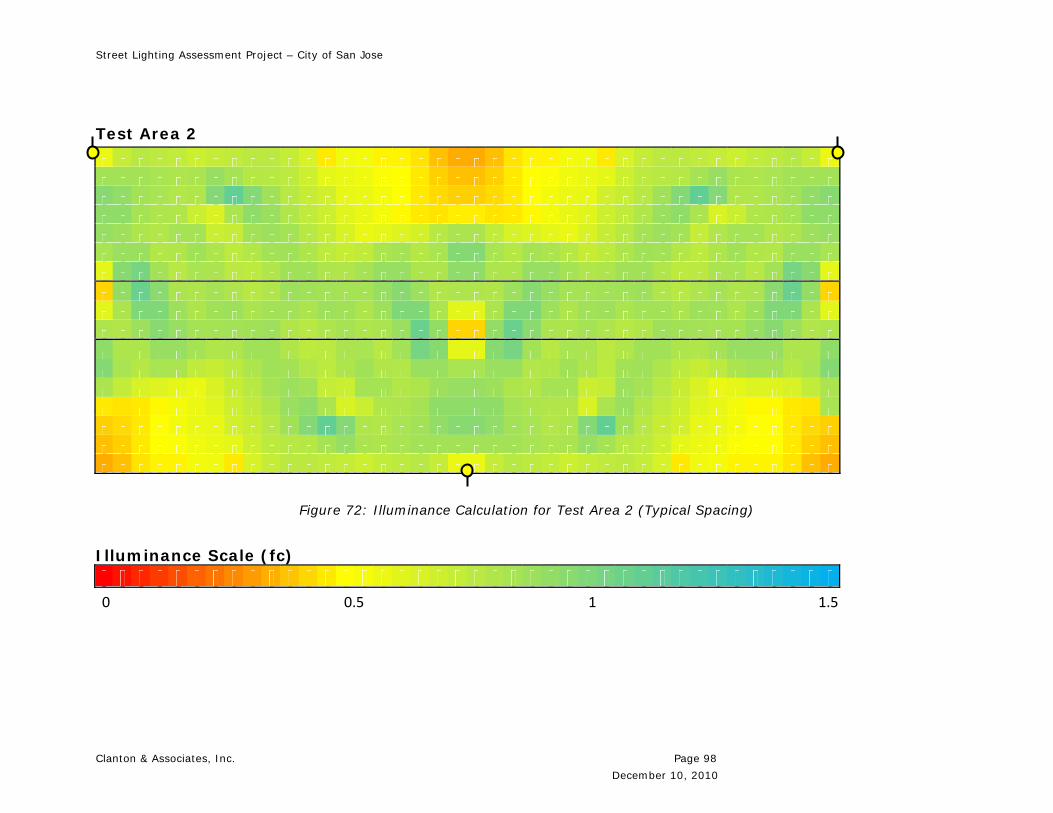
Street Lighting Assessment Project – City of San Jose
Clanton & Associates, Inc. Page 98
December 10, 2010
Test Area 2
Figure 72: Illuminance Calculation for Test Area 2 (Typical Spacing)
Illuminance Scale (fc)
0 0.5 1 1.5
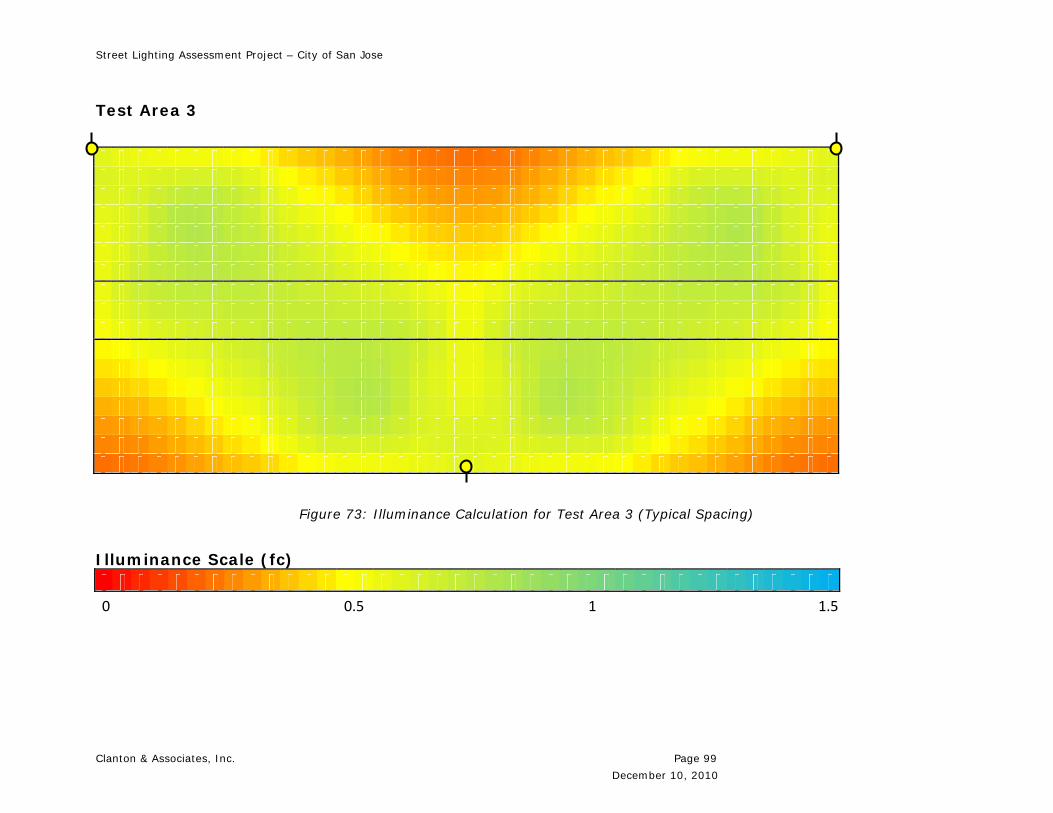
Street Lighting Assessment Project – City of San Jose
Clanton & Associates, Inc. Page 99
December 10, 2010
Test Area 3
Figure 73: Illuminance Calculation for Test Area 3 (Typical Spacing)
Illuminance Scale (fc)
0 0.5 1 1.5

Street Lighting Assessment Project – City of San Jose
Clanton & Associates, Inc. Page 100
December 10, 2010
Test Area 4
Figure 74: Illuminance Calculation for Test Area 4 (Typical Spacing)
Illuminance Scale (fc)
0 0.5 1 1.5

Street Lighting Assessment Project – City of San Jose
Clanton & Associates, Inc. Page 101
December 10, 2010
Test Area 5
Figure 75: Illuminance Calculation for Test Area 5 (Typical Spacing)
Illuminance Scale (fc)
0 0.5 1 1.5

Street Lighting Assessment Project – City of San Jose
Clanton & Associates, Inc. Page 102
December 10, 2010
Test Area 6
Figure 76: Illuminance Calculation for Test Area 6 (Typical Spacing)
Illuminance Scale (fc)
0 0.5 1 1.5

Street Lighting Assessment Project – City of San Jose
Clanton & Associates, Inc. Page 103
December 10, 2010

Street Lighting Assessment Project – City of San Jose
Clanton & Associates, Inc. Page 104
December 10, 2010
11.0 Appendix F: Subjective Survey Results
Ninety five percent confidence intervals were constructed around the mean score for each statement. These intervals were also compared across Test Areas. Significant differences for responses to the systems are determined by comparing confidence intervals. When the intervals do not overlap, the difference is considered statistically significant at the 95% confidence level.
It is important to note that a statistically significant difference refers to differences in results that most likely (with 95% certainty) did not occur by chance. It does not mean that the differences are significant in the practical sense of the word. Additionally, a difference that is not considered statistically significant does not mean that it may not be important.
The confidence intervals for all of the survey statements are shown in the following figures.
1.00
1.50
2.00
2.50
3.00
3.50
4.00
4.50
5.00
Are
a 1
Are
a 2
Are
a 3
Are
a 4
Are
a 5
Are
a 6
Are
a 1
Are
a 2
Are
a 3
Are
a 4
Are
a 5
Are
a 6
Are
a 1
Are
a 2
Are
a 3
Are
a 4
Are
a 5
Are
a 6
Are
a 1
Are
a 2
Are
a 3
Are
a 4
Are
a 5
Are
a 6
Are
a 1
Are
a 2
Are
a 3
Are
a 4
Are
a 5
Are
a 6
Are
a 1
Are
a 2
Are
a 3
Are
a 4
Are
a 5
Are
a 6
Are
a 1
Are
a 2
Are
a 3
Are
a 4
Are
a 5
Are
a 6
Are
a 1
Are
a 2
Are
a 3
Are
a 4
Are
a 5
Are
a 6
Are
a 1
Are
a 2
Are
a 3
Are
a 4
Are
a 5
Are
a 6
Are
a 1
Are
a 2
Are
a 3
Are
a 4
Are
a 5
Are
a 6
Are
a 1
Are
a 2
Are
a 3
Are
a 4
Are
a 5
Are
a 6
Are
a 1
Are
a 2
Are
a 3
Are
a 4
Are
a 5
Are
a 6
Are
a 1
Are
a 2
Are
a 3
Are
a 4
Are
a 5
Are
a 6
S1 S2 S3 S4 S5 S6 S7 S8 S9 S10 S11 S12 S13
Re
spo
nse
Valu
e
Area by Statement
San Jose Survey Group Night 1 and Night 2Night 1 Night 2
Figure 77: Composite Survey Results, Night 1 and Night 2

Street Lighting Assessment Project – City of San Jose
Clanton & Associates, Inc. Page 105
December 10, 2010
Night 1
1.00
1.50
2.00
2.50
3.00
3.50
4.00
4.50
5.00
Are
a 1
Are
a 2
Are
a 3
Are
a 4
Are
a 5
Are
a 6
Are
a 1
Are
a 2
Are
a 3
Are
a 4
Are
a 5
Are
a 6
Are
a 1
Are
a 2
Are
a 3
Are
a 4
Are
a 5
Are
a 6
Are
a 1
Are
a 2
Are
a 3
Are
a 4
Are
a 5
Are
a 6
Are
a 1
Are
a 2
Are
a 3
Are
a 4
Are
a 5
Are
a 6
Are
a 1
Are
a 2
Are
a 3
Are
a 4
Are
a 5
Are
a 6
Are
a 1
Are
a 2
Are
a 3
Are
a 4
Are
a 5
Are
a 6
Are
a 1
Are
a 2
Are
a 3
Are
a 4
Are
a 5
Are
a 6
Are
a 1
Are
a 2
Are
a 3
Are
a 4
Are
a 5
Are
a 6
Are
a 1
Are
a 2
Are
a 3
Are
a 4
Are
a 5
Are
a 6
Are
a 1
Are
a 2
Are
a 3
Are
a 4
Are
a 5
Are
a 6
Are
a 1
Are
a 2
Are
a 3
Are
a 4
Are
a 5
Are
a 6
Are
a 1
Are
a 2
Are
a 3
Are
a 4
Are
a 5
Are
a 6
S1 S2 S3 S4 S5 S6 S7 S8 S9 S10 S11 S12 S13
Re
spo
nse
Valu
e
Area by Statement
San Jose Survey Night 1
Figure 78: Composite Survey Results, Night 1

Street Lighting Assessment Project – City of San Jose
Clanton & Associates, Inc. Page 106
December 10, 2010
1.00
1.50
2.00
2.50
3.00
3.50
4.00
4.50
5.00
Are
a 1
Are
a 2
Are
a 3
Are
a 4
Are
a 5
Are
a 6
Are
a 1
Are
a 2
Are
a 3
Are
a 4
Are
a 5
Are
a 6
Are
a 1
Are
a 2
Are
a 3
Are
a 4
Are
a 5
Are
a 6
S1 S2 S3
Re
sp
onse V
alu
e
Area by Statement
Figure 79: Night 1 Survey Results, S1-3
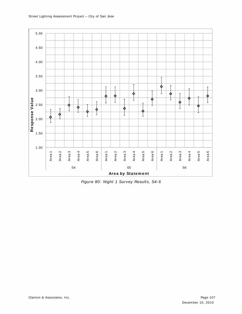
Street Lighting Assessment Project – City of San Jose
Clanton & Associates, Inc. Page 107
December 10, 2010
1.00
1.50
2.00
2.50
3.00
3.50
4.00
4.50
5.00
Are
a 1
Are
a 2
Are
a 3
Are
a 4
Are
a 5
Are
a 6
Are
a 1
Are
a 2
Are
a 3
Are
a 4
Are
a 5
Are
a 6
Are
a 1
Are
a 2
Are
a 3
Are
a 4
Are
a 5
Are
a 6
S4 S5 S6
Re
sp
onse V
alu
e
Area by Statement Figure 80: Night 1 Survey Results, S4-6
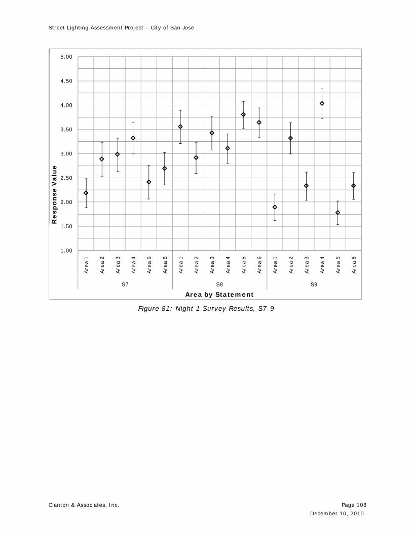
Street Lighting Assessment Project – City of San Jose
Clanton & Associates, Inc. Page 108
December 10, 2010
1.00
1.50
2.00
2.50
3.00
3.50
4.00
4.50
5.00
Are
a 1
Are
a 2
Are
a 3
Are
a 4
Are
a 5
Are
a 6
Are
a 1
Are
a 2
Are
a 3
Are
a 4
Are
a 5
Are
a 6
Are
a 1
Are
a 2
Are
a 3
Are
a 4
Are
a 5
Are
a 6
S7 S8 S9
Re
sp
onse V
alu
e
Area by Statement Figure 81: Night 1 Survey Results, S7-9

Street Lighting Assessment Project – City of San Jose
Clanton & Associates, Inc. Page 109
December 10, 2010
1.00
1.50
2.00
2.50
3.00
3.50
4.00
4.50
5.00
Are
a 1
Are
a 2
Are
a 3
Are
a 4
Are
a 5
Are
a 6
Are
a 1
Are
a 2
Are
a 3
Are
a 4
Are
a 5
Are
a 6
Are
a 1
Are
a 2
Are
a 3
Are
a 4
Are
a 5
Are
a 6
Are
a 1
Are
a 2
Are
a 3
Are
a 4
Are
a 5
Are
a 6
S10 S11 S12 S13
Re
sp
onse
Va
lue
Area by Statement Figure 82: Night 1 Survey Results, S10-13

Street Lighting Assessment Project – City of San Jose
Clanton & Associates, Inc. Page 110
December 10, 2010
Night 2
1.00
1.50
2.00
2.50
3.00
3.50
4.00
4.50
5.00
Are
a 1
Are
a 2
Are
a 3
Are
a 4
Are
a 5
Are
a 6
Are
a 1
Are
a 2
Are
a 3
Are
a 4
Are
a 5
Are
a 6
Are
a 1
Are
a 2
Are
a 3
Are
a 4
Are
a 5
Are
a 6
Are
a 1
Are
a 2
Are
a 3
Are
a 4
Are
a 5
Are
a 6
Are
a 1
Are
a 2
Are
a 3
Are
a 4
Are
a 5
Are
a 6
Are
a 1
Are
a 2
Are
a 3
Are
a 4
Are
a 5
Are
a 6
Are
a 1
Are
a 2
Are
a 3
Are
a 4
Are
a 5
Are
a 6
Are
a 1
Are
a 2
Are
a 3
Are
a 4
Are
a 5
Are
a 6
Are
a 1
Are
a 2
Are
a 3
Are
a 4
Are
a 5
Are
a 6
Are
a 1
Are
a 2
Are
a 3
Are
a 4
Are
a 5
Are
a 6
Are
a 1
Are
a 2
Are
a 3
Are
a 4
Are
a 5
Are
a 6
Are
a 1
Are
a 2
Are
a 3
Are
a 4
Are
a 5
Are
a 6
Are
a 1
Are
a 2
Are
a 3
Are
a 4
Are
a 5
Are
a 6
S1 S2 S3 S4 S5 S6 S7 S8 S9 S10 S11 S12 S13
Re
spo
nse
Valu
e
Area by Statement
San Jose Survey Night 2
Figure 83: Composite Survey Results, Night 2

Street Lighting Assessment Project – City of San Jose
Clanton & Associates, Inc. Page 111
December 10, 2010
1.00
1.50
2.00
2.50
3.00
3.50
4.00
4.50
5.00
Are
a 1
Are
a 2
Are
a 3
Are
a 4
Are
a 5
Are
a 6
Are
a 1
Are
a 2
Are
a 3
Are
a 4
Are
a 5
Are
a 6
Are
a 1
Are
a 2
Are
a 3
Are
a 4
Are
a 5
Are
a 6
S1 S2 S3
Re
sp
onse V
alu
e
Area by Statement Figure 84: Night 2 Survey Results, S1-3

Street Lighting Assessment Project – City of San Jose
Clanton & Associates, Inc. Page 112
December 10, 2010
1.00
1.50
2.00
2.50
3.00
3.50
4.00
4.50
5.00
Are
a 1
Are
a 2
Are
a 3
Are
a 4
Are
a 5
Are
a 6
Are
a 1
Are
a 2
Are
a 3
Are
a 4
Are
a 5
Are
a 6
Are
a 1
Are
a 2
Are
a 3
Are
a 4
Are
a 5
Are
a 6
S4 S5 S6
Re
sp
onse V
alu
e
Area by Statement Figure 85: Night 2 Survey Results, S4-6
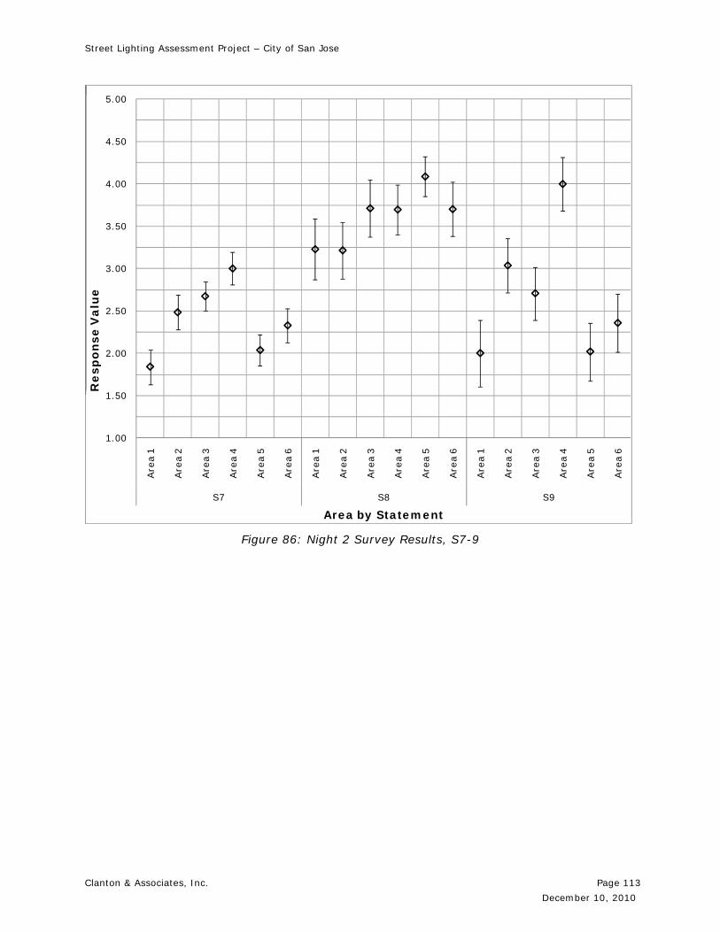
Street Lighting Assessment Project – City of San Jose
Clanton & Associates, Inc. Page 113
December 10, 2010
1.00
1.50
2.00
2.50
3.00
3.50
4.00
4.50
5.00
Are
a 1
Are
a 2
Are
a 3
Are
a 4
Are
a 5
Are
a 6
Are
a 1
Are
a 2
Are
a 3
Are
a 4
Are
a 5
Are
a 6
Are
a 1
Are
a 2
Are
a 3
Are
a 4
Are
a 5
Are
a 6
S7 S8 S9
Re
sp
onse V
alu
e
Area by Statement Figure 86: Night 2 Survey Results, S7-9

Street Lighting Assessment Project – City of San Jose
Clanton & Associates, Inc. Page 114
December 10, 2010
1.00
1.50
2.00
2.50
3.00
3.50
4.00
4.50
5.00
Are
a 1
Are
a 2
Are
a 3
Are
a 4
Are
a 5
Are
a 6
Are
a 1
Are
a 2
Are
a 3
Are
a 4
Are
a 5
Are
a 6
Are
a 1
Are
a 2
Are
a 3
Are
a 4
Are
a 5
Are
a 6
Are
a 1
Are
a 2
Are
a 3
Are
a 4
Are
a 5
Are
a 6
S10 S11 S12 S13
Re
sp
onse
Va
lue
Area by Statement Figure 87: Night 1 Survey Results, S10-13

Street Lighting Assessment Project – City of San Jose
Clanton & Associates, Inc. Page 115
December 10, 2010
12.0 Appendix G: Control Systems
A centralized lighting control system performs the task of communicating with each luminaire. Regardless of the specific manufacturer or technology, each control system configuration requires a device on each of the lights or a circuit of lights. Additionally, there is a base station of sorts that communicates with each of the devices. There are far fewer base stations than there are devices. The last required component is a software program. The software allows for the user to interface, via a web portal, to the base station, which then communicates to each of the devices.
Depending on the scope and size of the lights being controlled, there are different control technologies that may work better than others.
Radio Frequency (RF)
A RF system, through a mesh network, can work with very large quantities of lights. The mesh network allows for a control signal to be traversed through multiple points, instead of one single control hub. Installing a RF device at each light does not require rewiring. The RF device is installed via a photocell receptacle already on place on the luminaire. This type, because of the device to device communication, is not limited by topography.
Pros: Not labor intensive. Cons: Concerns of spectrum management. There is a wide range of frequencies that
are allowed when using radio frequency. Determining the frequency with the least amount of noise will improve the communication between the luminaires.
Power Line Carrier (PLC) A PLC system communicates using existing conductors that are also used for electric power transmission. PLC communication can be used at each of the stages of electrical power distribution: high voltage transmission lines, distributed medium voltage, and lower voltages. Usually the signal is halted at the transformer. In the case of multiple transformers, multiple PLC technologies are used and bridged together to cover the needed area.
Pros: Direct communication between luminaires. Cons: Quality of power. Often in outdoor lighting, the power quality can be ‘dirty’,
meaning that there are consistent fluctuations in voltage. This can cause equipment failure if the selected equipment is not rated to handle a range of voltages.
Figure 88: Examples of RF Devices for Lighting Equipment.

Street Lighting Assessment Project – City of San Jose
Clanton & Associates, Inc. Page 116
December 10, 2010
Once a system is configured and all of the lights are connected and communicating properly, the capabilities of the system are immense. There are several manufacturers available that offer a centralized control system. Some of the benefits of these manufacturers include:
Control of on/off times Energy consumption metering (revenue grade) Develop adaptive lighting protocols to correspond with traffic and pedestrian flows Ability to control up to 100,000 points of street light control Logging of operating hours for each individual lamp Remotely program output of entire street light network Effectively plan lamp luminaire locations and installations Reduce maintenance costs and increase public safety through the development of
proactive maintenance schedules – alerts by email for lamp failures Quickly generate reports for installation planning, maintenance programs and energy
usage

Street Lighting Assessment Project – City of San Jose
Clanton & Associates, Inc. Page 117
December 10, 2010
13.0 Appendix H: Luminance Adjustment Factors
LPS Luminance Adjustment FactorsPhotopic 0.010 0.020 0.030 0.040 0.050 0.060 0.070 0.080 0.090 0.100 0.110 0.120 0.130 0.140 0.150 0.160 0.170 0.180 0.190
Mesopic 0.003 0.008 0.014 0.020 0.026 0.033 0.040 0.047 0.054 0.061 0.068 0.076 0.083 0.091 0.099 0.107 0.115 0.123 0.131
Photopic 0.200 0.210 0.220 0.230 0.240 0.250 0.260 0.270 0.280 0.290 0.300 0.310 0.320 0.330 0.340 0.350 0.360 0.370 0.380 0.390
Mesopic 0.139 0.147 0.155 0.163 0.172 0.180 0.188 0.197 0.205 0.214 0.223 0.231 0.240 0.249 0.257 0.266 0.275 0.284 0.293 0.301
Photopic 0.400 0.410 0.420 0.430 0.440 0.450 0.460 0.470 0.480 0.490 0.500 0.510 0.520 0.530 0.540 0.550 0.560 0.570 0.580 0.590
Mesopic 0.310 0.319 0.328 0.337 0.346 0.355 0.365 0.374 0.383 0.392 0.401 0.411 0.420 0.429 0.438 0.448 0.457 0.466 0.476 0.485
Photopic 0.600 0.610 0.620 0.630 0.640 0.650 0.660 0.670 0.680 0.690 0.700 0.710 0.720 0.730 0.740 0.750 0.760 0.770 0.780 0.790
Mesopic 0.495 0.504 0.513 0.523 0.532 0.542 0.552 0.561 0.571 0.580 0.590 0.599 0.609 0.619 0.628 0.638 0.648 0.658 0.667 0.677
Photopic 0.800 0.810 0.820 0.830 0.840 0.850 0.860 0.870 0.880 0.890 0.900 0.910 0.920 0.930 0.940 0.950 0.960 0.970 0.980 0.990
Mesopic 0.687 0.697 0.706 0.716 0.726 0.736 0.746 0.756 0.765 0.775 0.785 0.795 0.805 0.815 0.825 0.835 0.845 0.855 0.865 0.875
Photopic 1.000 1.010 1.020 1.030 1.040 1.050 1.060 1.070 1.080 1.090 1.100 1.110 1.120 1.130 1.140 1.150 1.160 1.170 1.180 1.190
Mesopic 0.885 0.895 0.905 0.915 0.925 0.935 0.946 0.956 0.966 0.976 0.986 0.996 1.006 1.017 1.027 1.037 1.047 1.057 1.068 1.078
Photopic 1.200 1.210 1.220 1.230 1.240 1.250 1.260 1.270 1.280 1.290 1.300 1.310 1.320 1.330 1.340 1.350 1.360 1.370 1.380 1.390
Mesopic 1.088 1.098 1.109 1.119 1.129 1.140 1.150 1.160 1.171 1.181 1.191 1.202 1.212 1.222 1.233 1.243 1.254 1.264 1.274 1.285
Photopic 1.400 1.410 1.420 1.430 1.440 1.450 1.460 1.470 1.480 1.490 1.500 1.510 1.520 1.530 1.540 1.550 1.560 1.570 1.580 1.590
Mesopic 1.295 1.306 1.316 1.327 1.337 1.348 1.358 1.369 1.379 1.390 1.400 1.411 1.421 1.432 1.442 1.453 1.463 1.474 1.485 1.495
Photopic 1.600 1.610 1.620 1.630 1.640 1.650 1.660 1.670 1.680 1.690 1.700 1.710 1.720 1.730 1.740 1.750 1.760 1.770 1.780 1.790
Mesopic 1.506 1.516 1.527 1.538 1.548 1.559 1.569 1.580 1.591 1.601 1.612 1.623 1.633 1.644 1.655 1.666 1.676 1.687 1.698 1.708
Photopic 1.800 1.810 1.820 1.830 1.840 1.850 1.860 1.870 1.880 1.890 1.900 1.910 1.920 1.930 1.940 1.950 1.960 1.970 1.980 1.990
Mesopic 1.719 1.730 1.741 1.751 1.762 1.773 1.784 1.795 1.805 1.816 1.827 1.838 1.849 1.859 1.870 1.881 1.892 1.903 1.914 1.924
Photopic 2.000 2.010 2.020 2.030 2.040 2.050 2.060 2.070 2.080 2.090 2.100 2.110 2.120 2.130 2.140 2.150 2.160 2.170 2.180 2.190
Mesopic 1.935 1.946 1.957 1.968 1.979 1.990 2.001 2.012 2.022 2.033 2.044 2.055 2.066 2.077 2.088 2.099 2.110 2.121 2.132 2.143
Photopic 2.200 2.210 2.220 2.230 2.240 2.250 2.260 2.270 2.280 2.290 2.300 2.310 2.320 2.330 2.340 2.350 2.360 2.370 2.380 2.390
Mesopic 2.154 2.165 2.176 2.187 2.198 2.209 2.220 2.231 2.242 2.253 2.264 2.275 2.286 2.297 2.308 2.319 2.330 2.341 2.352 2.363
Photopic 2.400 2.410 2.420 2.430 2.440 2.450 2.460 2.470 2.480 2.490 2.500 2.510 2.520 2.530 2.540 2.550 2.560 2.570 2.580 2.590
Mesopic 2.374 2.386 2.397 2.408 2.419 2.430 2.441 2.452 2.463 2.474 2.486 2.497 2.508 2.519 2.530 2.541 2.552 2.564 2.575 2.586
Photopic 2.600 2.610 2.620 2.630 2.640 2.650 2.660 2.670 2.680 2.690 2.700 2.710 2.720 2.730 2.740 2.750 2.760 2.770 2.780 2.790
Mesopic 2.597 2.608 2.620 2.631 2.642 2.653 2.664 2.676 2.687 2.698 2.709 2.720 2.732 2.743 2.754 2.765 2.777 2.788 2.799 2.810
Photopic 2.800 2.810 2.820 2.830 2.840 2.850 2.860 2.870 2.880 2.890 2.900 2.910 2.920 2.930 2.940 2.950 2.960 2.970 2.980 2.990
Mesopic 2.822 2.833 2.844 2.855 2.867 2.878 2.889 2.901 2.912 2.923 2.935 2.946 2.957 2.968 2.980 2.991 3.002 3.014 3.025 3.036

Street Lighting Assessment Project – City of San Jose
Clanton & Associates, Inc. Page 118
December 10, 2010
HPS Luminance Adjustment FactorsPhotopic 0.010 0.020 0.030 0.040 0.050 0.060 0.070 0.080 0.090 0.100 0.110 0.120 0.130 0.140 0.150 0.160 0.170 0.180 0.190
Mesopic 0.007 0.015 0.022 0.031 0.039 0.047 0.056 0.064 0.073 0.082 0.090 0.099 0.108 0.117 0.126 0.135 0.144 0.153 0.162
Photopic 0.200 0.210 0.220 0.230 0.240 0.250 0.260 0.270 0.280 0.290 0.300 0.310 0.320 0.330 0.340 0.350 0.360 0.370 0.380 0.390
Mesopic 0.171 0.180 0.189 0.198 0.208 0.217 0.226 0.235 0.245 0.254 0.263 0.273 0.282 0.291 0.301 0.310 0.319 0.329 0.338 0.348
Photopic 0.400 0.410 0.420 0.430 0.440 0.450 0.460 0.470 0.480 0.490 0.500 0.510 0.520 0.530 0.540 0.550 0.560 0.570 0.580 0.590
Mesopic 0.357 0.367 0.376 0.386 0.395 0.405 0.415 0.424 0.434 0.443 0.453 0.463 0.472 0.482 0.491 0.501 0.511 0.520 0.530 0.540
Photopic 0.600 0.610 0.620 0.630 0.640 0.650 0.660 0.670 0.680 0.690 0.700 0.710 0.720 0.730 0.740 0.750 0.760 0.770 0.780 0.790
Mesopic 0.550 0.559 0.569 0.579 0.589 0.598 0.608 0.618 0.628 0.637 0.647 0.657 0.667 0.677 0.686 0.696 0.706 0.716 0.726 0.736
Photopic 0.800 0.810 0.820 0.830 0.840 0.850 0.860 0.870 0.880 0.890 0.900 0.910 0.920 0.930 0.940 0.950 0.960 0.970 0.980 0.990
Mesopic 0.746 0.755 0.765 0.775 0.785 0.795 0.805 0.815 0.825 0.835 0.845 0.855 0.865 0.875 0.884 0.894 0.904 0.914 0.924 0.934
Photopic 1.000 1.010 1.020 1.030 1.040 1.050 1.060 1.070 1.080 1.090 1.100 1.110 1.120 1.130 1.140 1.150 1.160 1.170 1.180 1.190
Mesopic 0.944 0.954 0.964 0.974 0.984 0.994 1.005 1.015 1.025 1.035 1.045 1.055 1.065 1.075 1.085 1.095 1.105 1.115 1.125 1.135
Photopic 1.200 1.210 1.220 1.230 1.240 1.250 1.260 1.270 1.280 1.290 1.300 1.310 1.320 1.330 1.340 1.350 1.360 1.370 1.380 1.390
Mesopic 1.145 1.156 1.166 1.176 1.186 1.196 1.206 1.216 1.226 1.237 1.247 1.257 1.267 1.277 1.287 1.298 1.308 1.318 1.328 1.338
Photopic 1.400 1.410 1.420 1.430 1.440 1.450 1.460 1.470 1.480 1.490 1.500 1.510 1.520 1.530 1.540 1.550 1.560 1.570 1.580 1.590
Mesopic 1.348 1.359 1.369 1.379 1.389 1.399 1.410 1.420 1.430 1.440 1.450 1.461 1.471 1.481 1.491 1.502 1.512 1.522 1.532 1.543
Photopic 1.600 1.610 1.620 1.630 1.640 1.650 1.660 1.670 1.680 1.690 1.700 1.710 1.720 1.730 1.740 1.750 1.760 1.770 1.780 1.790
Mesopic 1.553 1.563 1.573 1.584 1.594 1.604 1.615 1.625 1.635 1.645 1.656 1.666 1.676 1.687 1.697 1.707 1.718 1.728 1.738 1.749
Photopic 1.800 1.810 1.820 1.830 1.840 1.850 1.860 1.870 1.880 1.890 1.900 1.910 1.920 1.930 1.940 1.950 1.960 1.970 1.980 1.990
Mesopic 1.759 1.769 1.780 1.790 1.800 1.811 1.821 1.831 1.842 1.852 1.862 1.873 1.883 1.893 1.904 1.914 1.924 1.935 1.945 1.956
Photopic 2.000 2.010 2.020 2.030 2.040 2.050 2.060 2.070 2.080 2.090 2.100 2.110 2.120 2.130 2.140 2.150 2.160 2.170 2.180 2.190
Mesopic 1.966 1.976 1.987 1.997 2.008 2.018 2.028 2.039 2.049 2.060 2.070 2.080 2.091 2.101 2.112 2.122 2.133 2.143 2.153 2.164
Photopic 2.200 2.210 2.220 2.230 2.240 2.250 2.260 2.270 2.280 2.290 2.300 2.310 2.320 2.330 2.340 2.350 2.360 2.370 2.380 2.390
Mesopic 2.174 2.185 2.195 2.206 2.216 2.227 2.237 2.247 2.258 2.268 2.279 2.289 2.300 2.310 2.321 2.331 2.342 2.352 2.363 2.373
Photopic 2.400 2.410 2.420 2.430 2.440 2.450 2.460 2.470 2.480 2.490 2.500 2.510 2.520 2.530 2.540 2.550 2.560 2.570 2.580 2.590
Mesopic 2.384 2.394 2.405 2.415 2.426 2.436 2.447 2.457 2.468 2.478 2.489 2.499 2.510 2.520 2.531 2.541 2.552 2.562 2.573 2.583
Photopic 2.600 2.610 2.620 2.630 2.640 2.650 2.660 2.670 2.680 2.690 2.700 2.710 2.720 2.730 2.740 2.750 2.760 2.770 2.780 2.790
Mesopic 2.594 2.604 2.615 2.625 2.636 2.647 2.657 2.668 2.678 2.689 2.699 2.710 2.720 2.731 2.741 2.752 2.763 2.773 2.784 2.794
Photopic 2.800 2.810 2.820 2.830 2.840 2.850 2.860 2.870 2.880 2.890 2.900 2.910 2.920 2.930 2.940 2.950 2.960 2.970 2.980 2.990
Mesopic 2.805 2.815 2.826 2.837 2.847 2.858 2.868 2.879 2.890 2.900 2.911 2.921 2.932 2.943 2.953 2.964 2.974 2.985 2.996 3.006

Street Lighting Assessment Project – City of San Jose
Clanton & Associates, Inc. Page 119
December 10, 2010
3500K Luminance Adjustment FactorsPhotopic 0.010 0.020 0.030 0.040 0.050 0.060 0.070 0.080 0.090 0.100 0.110 0.120 0.130 0.140 0.150 0.160 0.170 0.180 0.190
Mesopic 0.012 0.023 0.034 0.045 0.056 0.067 0.077 0.088 0.099 0.110 0.120 0.131 0.141 0.152 0.163 0.173 0.184 0.194 0.205
Photopic 0.200 0.210 0.220 0.230 0.240 0.250 0.260 0.270 0.280 0.290 0.300 0.310 0.320 0.330 0.340 0.350 0.360 0.370 0.380 0.390
Mesopic 0.215 0.226 0.236 0.247 0.257 0.268 0.278 0.288 0.299 0.309 0.319 0.330 0.340 0.351 0.361 0.371 0.382 0.392 0.402 0.412
Photopic 0.400 0.410 0.420 0.430 0.440 0.450 0.460 0.470 0.480 0.490 0.500 0.510 0.520 0.530 0.540 0.550 0.560 0.570 0.580 0.590
Mesopic 0.423 0.433 0.443 0.454 0.464 0.474 0.484 0.495 0.505 0.515 0.525 0.536 0.546 0.556 0.566 0.576 0.587 0.597 0.607 0.617
Photopic 0.600 0.610 0.620 0.630 0.640 0.650 0.660 0.670 0.680 0.690 0.700 0.710 0.720 0.730 0.740 0.750 0.760 0.770 0.780 0.790
Mesopic 0.627 0.637 0.648 0.658 0.668 0.678 0.688 0.698 0.709 0.719 0.729 0.739 0.749 0.759 0.769 0.779 0.790 0.800 0.810 0.820
Photopic 0.800 0.810 0.820 0.830 0.840 0.850 0.860 0.870 0.880 0.890 0.900 0.910 0.920 0.930 0.940 0.950 0.960 0.970 0.980 0.990
Mesopic 0.830 0.840 0.850 0.860 0.870 0.880 0.890 0.901 0.911 0.921 0.931 0.941 0.951 0.961 0.971 0.981 0.991 1.001 1.011 1.021
Photopic 1.000 1.010 1.020 1.030 1.040 1.050 1.060 1.070 1.080 1.090 1.100 1.110 1.120 1.130 1.140 1.150 1.160 1.170 1.180 1.190
Mesopic 1.031 1.041 1.051 1.061 1.071 1.081 1.091 1.101 1.111 1.121 1.131 1.141 1.151 1.161 1.171 1.181 1.191 1.201 1.211 1.221
Photopic 1.200 1.210 1.220 1.230 1.240 1.250 1.260 1.270 1.280 1.290 1.300 1.310 1.320 1.330 1.340 1.350 1.360 1.370 1.380 1.390
Mesopic 1.231 1.241 1.251 1.261 1.271 1.281 1.291 1.301 1.311 1.321 1.331 1.341 1.351 1.361 1.371 1.381 1.391 1.401 1.411 1.421
Photopic 1.400 1.410 1.420 1.430 1.440 1.450 1.460 1.470 1.480 1.490 1.500 1.510 1.520 1.530 1.540 1.550 1.560 1.570 1.580 1.590
Mesopic 1.430 1.440 1.450 1.460 1.470 1.480 1.490 1.500 1.510 1.520 1.530 1.540 1.550 1.560 1.569 1.579 1.589 1.599 1.609 1.619
Photopic 1.600 1.610 1.620 1.630 1.640 1.650 1.660 1.670 1.680 1.690 1.700 1.710 1.720 1.730 1.740 1.750 1.760 1.770 1.780 1.790
Mesopic 1.629 1.639 1.649 1.659 1.668 1.678 1.688 1.698 1.708 1.718 1.728 1.738 1.748 1.757 1.767 1.777 1.787 1.797 1.807 1.817
Photopic 1.800 1.810 1.820 1.830 1.840 1.850 1.860 1.870 1.880 1.890 1.900 1.910 1.920 1.930 1.940 1.950 1.960 1.970 1.980 1.990
Mesopic 1.827 1.836 1.846 1.856 1.866 1.876 1.886 1.896 1.905 1.915 1.925 1.935 1.945 1.955 1.965 1.974 1.984 1.994 2.004 2.014
Photopic 2.000 2.010 2.020 2.030 2.040 2.050 2.060 2.070 2.080 2.090 2.100 2.110 2.120 2.130 2.140 2.150 2.160 2.170 2.180 2.190
Mesopic 2.024 2.033 2.043 2.053 2.063 2.073 2.083 2.092 2.102 2.112 2.122 2.132 2.142 2.151 2.161 2.171 2.181 2.191 2.200 2.210
Photopic 2.200 2.210 2.220 2.230 2.240 2.250 2.260 2.270 2.280 2.290 2.300 2.310 2.320 2.330 2.340 2.350 2.360 2.370 2.380 2.390
Mesopic 2.220 2.230 2.240 2.249 2.259 2.269 2.279 2.289 2.299 2.308 2.318 2.328 2.338 2.348 2.357 2.367 2.377 2.387 2.396 2.406
Photopic 2.400 2.410 2.420 2.430 2.440 2.450 2.460 2.470 2.480 2.490 2.500 2.510 2.520 2.530 2.540 2.550 2.560 2.570 2.580 2.590
Mesopic 2.416 2.426 2.436 2.445 2.455 2.465 2.475 2.485 2.494 2.504 2.514 2.524 2.533 2.543 2.553 2.563 2.572 2.582 2.592 2.602
Photopic 2.600 2.610 2.620 2.630 2.640 2.650 2.660 2.670 2.680 2.690 2.700 2.710 2.720 2.730 2.740 2.750 2.760 2.770 2.780 2.790
Mesopic 2.612 2.621 2.631 2.641 2.651 2.660 2.670 2.680 2.690 2.699 2.709 2.719 2.729 2.738 2.748 2.758 2.768 2.777 2.787 2.797
Photopic 2.800 2.810 2.820 2.830 2.840 2.850 2.860 2.870 2.880 2.890 2.900 2.910 2.920 2.930 2.940 2.950 2.960 2.970 2.980 2.990
Mesopic 2.807 2.816 2.826 2.836 2.846 2.855 2.865 2.875 2.885 2.894 2.904 2.914 2.923 2.933 2.943 2.953 2.962 2.972 2.982 2.992

Street Lighting Assessment Project – City of San Jose
Clanton & Associates, Inc. Page 120
December 10, 2010
4000K Luminance Adjustment FactorsPhotopic 0.010 0.020 0.030 0.040 0.050 0.060 0.070 0.080 0.090 0.100 0.110 0.120 0.130 0.140 0.150 0.160 0.170 0.180 0.190
Mesopic 0.013 0.025 0.037 0.049 0.061 0.072 0.084 0.095 0.106 0.118 0.129 0.140 0.151 0.162 0.173 0.184 0.195 0.206 0.217
Photopic 0.200 0.210 0.220 0.230 0.240 0.250 0.260 0.270 0.280 0.290 0.300 0.310 0.320 0.330 0.340 0.350 0.360 0.370 0.380 0.390
Mesopic 0.228 0.239 0.250 0.261 0.272 0.282 0.293 0.304 0.315 0.325 0.336 0.347 0.357 0.368 0.379 0.389 0.400 0.410 0.421 0.431
Photopic 0.400 0.410 0.420 0.430 0.440 0.450 0.460 0.470 0.480 0.490 0.500 0.510 0.520 0.530 0.540 0.550 0.560 0.570 0.580 0.590
Mesopic 0.442 0.453 0.463 0.474 0.484 0.495 0.505 0.515 0.526 0.536 0.547 0.557 0.568 0.578 0.588 0.599 0.609 0.619 0.630 0.640
Photopic 0.600 0.610 0.620 0.630 0.640 0.650 0.660 0.670 0.680 0.690 0.700 0.710 0.720 0.730 0.740 0.750 0.760 0.770 0.780 0.790
Mesopic 0.650 0.661 0.671 0.681 0.692 0.702 0.712 0.722 0.733 0.743 0.753 0.763 0.774 0.784 0.794 0.804 0.814 0.825 0.835 0.845
Photopic 0.800 0.810 0.820 0.830 0.840 0.850 0.860 0.870 0.880 0.890 0.900 0.910 0.920 0.930 0.940 0.950 0.960 0.970 0.980 0.990
Mesopic 0.855 0.865 0.876 0.886 0.896 0.906 0.916 0.926 0.936 0.946 0.957 0.967 0.977 0.987 0.997 1.007 1.017 1.027 1.037 1.047
Photopic 1.000 1.010 1.020 1.030 1.040 1.050 1.060 1.070 1.080 1.090 1.100 1.110 1.120 1.130 1.140 1.150 1.160 1.170 1.180 1.190
Mesopic 1.057 1.067 1.077 1.088 1.098 1.108 1.118 1.128 1.138 1.148 1.158 1.168 1.178 1.188 1.198 1.208 1.218 1.228 1.238 1.248
Photopic 1.200 1.210 1.220 1.230 1.240 1.250 1.260 1.270 1.280 1.290 1.300 1.310 1.320 1.330 1.340 1.350 1.360 1.370 1.380 1.390
Mesopic 1.258 1.267 1.277 1.287 1.297 1.307 1.317 1.327 1.337 1.347 1.357 1.367 1.377 1.387 1.397 1.406 1.416 1.426 1.436 1.446
Photopic 1.400 1.410 1.420 1.430 1.440 1.450 1.460 1.470 1.480 1.490 1.500 1.510 1.520 1.530 1.540 1.550 1.560 1.570 1.580 1.590
Mesopic 1.456 1.466 1.476 1.485 1.495 1.505 1.515 1.525 1.535 1.545 1.554 1.564 1.574 1.584 1.594 1.604 1.613 1.623 1.633 1.643
Photopic 1.600 1.610 1.620 1.630 1.640 1.650 1.660 1.670 1.680 1.690 1.700 1.710 1.720 1.730 1.740 1.750 1.760 1.770 1.780 1.790
Mesopic 1.653 1.663 1.672 1.682 1.692 1.702 1.712 1.721 1.731 1.741 1.751 1.760 1.770 1.780 1.790 1.800 1.809 1.819 1.829 1.839
Photopic 1.800 1.810 1.820 1.830 1.840 1.850 1.860 1.870 1.880 1.890 1.900 1.910 1.920 1.930 1.940 1.950 1.960 1.970 1.980 1.990
Mesopic 1.848 1.858 1.868 1.878 1.887 1.897 1.907 1.916 1.926 1.936 1.946 1.955 1.965 1.975 1.985 1.994 2.004 2.014 2.023 2.033
Photopic 2.000 2.010 2.020 2.030 2.040 2.050 2.060 2.070 2.080 2.090 2.100 2.110 2.120 2.130 2.140 2.150 2.160 2.170 2.180 2.190
Mesopic 2.043 2.052 2.062 2.072 2.081 2.091 2.101 2.111 2.120 2.130 2.140 2.149 2.159 2.169 2.178 2.188 2.197 2.207 2.217 2.226
Photopic 2.200 2.210 2.220 2.230 2.240 2.250 2.260 2.270 2.280 2.290 2.300 2.310 2.320 2.330 2.340 2.350 2.360 2.370 2.380 2.390
Mesopic 2.236 2.246 2.255 2.265 2.275 2.284 2.294 2.304 2.313 2.323 2.332 2.342 2.352 2.361 2.371 2.380 2.390 2.400 2.409 2.419
Photopic 2.400 2.410 2.420 2.430 2.440 2.450 2.460 2.470 2.480 2.490 2.500 2.510 2.520 2.530 2.540 2.550 2.560 2.570 2.580 2.590
Mesopic 2.429 2.438 2.448 2.457 2.467 2.476 2.486 2.496 2.505 2.515 2.524 2.534 2.544 2.553 2.563 2.572 2.582 2.591 2.601 2.610
Photopic 2.600 2.610 2.620 2.630 2.640 2.650 2.660 2.670 2.680 2.690 2.700 2.710 2.720 2.730 2.740 2.750 2.760 2.770 2.780 2.790
Mesopic 2.620 2.630 2.639 2.649 2.658 2.668 2.677 2.687 2.696 2.706 2.716 2.725 2.735 2.744 2.754 2.763 2.773 2.782 2.792 2.801
Photopic 2.800 2.810 2.820 2.830 2.840 2.850 2.860 2.870 2.880 2.890 2.900 2.910 2.920 2.930 2.940 2.950 2.960 2.970 2.980 2.990
Mesopic 2.811 2.820 2.830 2.839 2.849 2.858 2.868 2.877 2.887 2.896 2.906 2.915 2.925 2.934 2.944 2.953 2.963 2.972 2.982 2.991
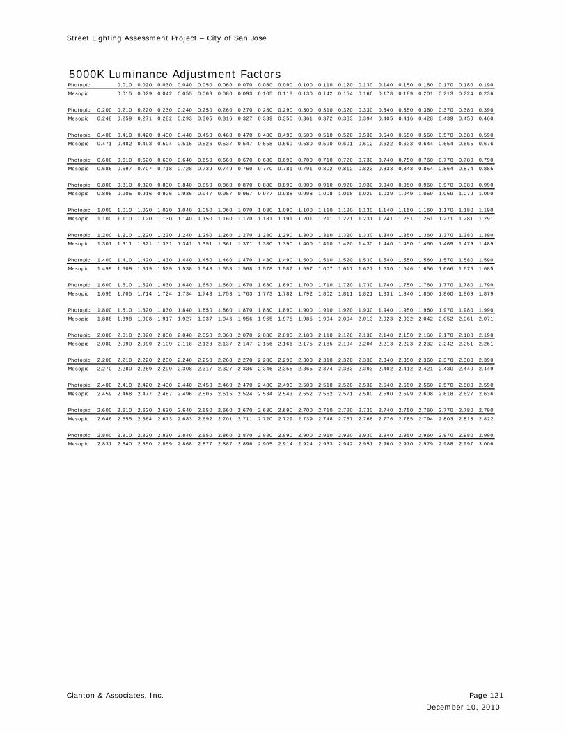
Street Lighting Assessment Project – City of San Jose
Clanton & Associates, Inc. Page 121
December 10, 2010
5000K Luminance Adjustment FactorsPhotopic 0.010 0.020 0.030 0.040 0.050 0.060 0.070 0.080 0.090 0.100 0.110 0.120 0.130 0.140 0.150 0.160 0.170 0.180 0.190
Mesopic 0.015 0.029 0.042 0.055 0.068 0.080 0.093 0.105 0.118 0.130 0.142 0.154 0.166 0.178 0.189 0.201 0.213 0.224 0.236
Photopic 0.200 0.210 0.220 0.230 0.240 0.250 0.260 0.270 0.280 0.290 0.300 0.310 0.320 0.330 0.340 0.350 0.360 0.370 0.380 0.390
Mesopic 0.248 0.259 0.271 0.282 0.293 0.305 0.316 0.327 0.339 0.350 0.361 0.372 0.383 0.394 0.405 0.416 0.428 0.439 0.450 0.460
Photopic 0.400 0.410 0.420 0.430 0.440 0.450 0.460 0.470 0.480 0.490 0.500 0.510 0.520 0.530 0.540 0.550 0.560 0.570 0.580 0.590
Mesopic 0.471 0.482 0.493 0.504 0.515 0.526 0.537 0.547 0.558 0.569 0.580 0.590 0.601 0.612 0.622 0.633 0.644 0.654 0.665 0.676
Photopic 0.600 0.610 0.620 0.630 0.640 0.650 0.660 0.670 0.680 0.690 0.700 0.710 0.720 0.730 0.740 0.750 0.760 0.770 0.780 0.790
Mesopic 0.686 0.697 0.707 0.718 0.728 0.739 0.749 0.760 0.770 0.781 0.791 0.802 0.812 0.823 0.833 0.843 0.854 0.864 0.874 0.885
Photopic 0.800 0.810 0.820 0.830 0.840 0.850 0.860 0.870 0.880 0.890 0.900 0.910 0.920 0.930 0.940 0.950 0.960 0.970 0.980 0.990
Mesopic 0.895 0.905 0.916 0.926 0.936 0.947 0.957 0.967 0.977 0.988 0.998 1.008 1.018 1.029 1.039 1.049 1.059 1.069 1.079 1.090
Photopic 1.000 1.010 1.020 1.030 1.040 1.050 1.060 1.070 1.080 1.090 1.100 1.110 1.120 1.130 1.140 1.150 1.160 1.170 1.180 1.190
Mesopic 1.100 1.110 1.120 1.130 1.140 1.150 1.160 1.170 1.181 1.191 1.201 1.211 1.221 1.231 1.241 1.251 1.261 1.271 1.281 1.291
Photopic 1.200 1.210 1.220 1.230 1.240 1.250 1.260 1.270 1.280 1.290 1.300 1.310 1.320 1.330 1.340 1.350 1.360 1.370 1.380 1.390
Mesopic 1.301 1.311 1.321 1.331 1.341 1.351 1.361 1.371 1.380 1.390 1.400 1.410 1.420 1.430 1.440 1.450 1.460 1.469 1.479 1.489
Photopic 1.400 1.410 1.420 1.430 1.440 1.450 1.460 1.470 1.480 1.490 1.500 1.510 1.520 1.530 1.540 1.550 1.560 1.570 1.580 1.590
Mesopic 1.499 1.509 1.519 1.529 1.538 1.548 1.558 1.568 1.578 1.587 1.597 1.607 1.617 1.627 1.636 1.646 1.656 1.666 1.675 1.685
Photopic 1.600 1.610 1.620 1.630 1.640 1.650 1.660 1.670 1.680 1.690 1.700 1.710 1.720 1.730 1.740 1.750 1.760 1.770 1.780 1.790
Mesopic 1.695 1.705 1.714 1.724 1.734 1.743 1.753 1.763 1.773 1.782 1.792 1.802 1.811 1.821 1.831 1.840 1.850 1.860 1.869 1.879
Photopic 1.800 1.810 1.820 1.830 1.840 1.850 1.860 1.870 1.880 1.890 1.900 1.910 1.920 1.930 1.940 1.950 1.960 1.970 1.980 1.990
Mesopic 1.888 1.898 1.908 1.917 1.927 1.937 1.946 1.956 1.965 1.975 1.985 1.994 2.004 2.013 2.023 2.032 2.042 2.052 2.061 2.071
Photopic 2.000 2.010 2.020 2.030 2.040 2.050 2.060 2.070 2.080 2.090 2.100 2.110 2.120 2.130 2.140 2.150 2.160 2.170 2.180 2.190
Mesopic 2.080 2.090 2.099 2.109 2.118 2.128 2.137 2.147 2.156 2.166 2.175 2.185 2.194 2.204 2.213 2.223 2.232 2.242 2.251 2.261
Photopic 2.200 2.210 2.220 2.230 2.240 2.250 2.260 2.270 2.280 2.290 2.300 2.310 2.320 2.330 2.340 2.350 2.360 2.370 2.380 2.390
Mesopic 2.270 2.280 2.289 2.299 2.308 2.317 2.327 2.336 2.346 2.355 2.365 2.374 2.383 2.393 2.402 2.412 2.421 2.430 2.440 2.449
Photopic 2.400 2.410 2.420 2.430 2.440 2.450 2.460 2.470 2.480 2.490 2.500 2.510 2.520 2.530 2.540 2.550 2.560 2.570 2.580 2.590
Mesopic 2.459 2.468 2.477 2.487 2.496 2.505 2.515 2.524 2.534 2.543 2.552 2.562 2.571 2.580 2.590 2.599 2.608 2.618 2.627 2.636
Photopic 2.600 2.610 2.620 2.630 2.640 2.650 2.660 2.670 2.680 2.690 2.700 2.710 2.720 2.730 2.740 2.750 2.760 2.770 2.780 2.790
Mesopic 2.646 2.655 2.664 2.673 2.683 2.692 2.701 2.711 2.720 2.729 2.739 2.748 2.757 2.766 2.776 2.785 2.794 2.803 2.813 2.822
Photopic 2.800 2.810 2.820 2.830 2.840 2.850 2.860 2.870 2.880 2.890 2.900 2.910 2.920 2.930 2.940 2.950 2.960 2.970 2.980 2.990
Mesopic 2.831 2.840 2.850 2.859 2.868 2.877 2.887 2.896 2.905 2.914 2.924 2.933 2.942 2.951 2.960 2.970 2.979 2.988 2.997 3.006

Street Lighting Assessment Project – City of San Jose
Clanton & Associates, Inc. Page 122
December 10, 2010
14.0 References
1 Lewis, Alan. “Visual Performance as a Function of Spectral Power Distribution of Light Sources at Luminances Used for General Outdoor Lighting.” JIES, Winter 1999, Vol. 28, No.1. Illuminating Engineering Society of North America, New York. 2 Lewis, Alan. “Equating Light Sources for Visual Performance at Low Luminances.” JIES, Winter 1998. Illuminating Engineering Society of North America, New York. 3 Lewin, Ian. “Visibility Factors in Outdoor Lighting Design, part 2.” The Lighting Journal, Early 2000. Institution of Lighting Engineers, Rugby, UK. 4 IESNA TM-12. “Spectral Effects of Lighting on Visual Performance at Mesopic Light Levels.” Illuminating Engineering Society of North America. 2006. New York, New York.
5 Advanced Lighting Guidelines. New Buildings Institute, Inc. 2003. 6 Clanton & Associates, Inc, Virginia Tech Transportation Institute. “Street Lighting Survey for Commercial Areas in the Municipality of Anchorage.” Municipality of Anchorage. 2009
7 Clanton & Associates, Inc, Emerging Technologies Associates, Inc, Virginia Tech Transportation Institute. “Advanced Street Lighting Technologies Assessment Project – City of San Diego.” San Diego Gas and Electric. 2010.
8 IESNA RP-8. “Recommended Practice for Street Lighting.” Illuminating Engineering Society of North America. 2005. New York, New York.
9 IESNA RP-8. “Recommended Practice for Street Lighting.” Illuminating Engineering Society of North America. 2005. New York, New York.
10 Clanton & Associates, Inc, Virginia Tech Transportation Institute. “Street Lighting Survey for Commercial Areas in the Municipality of Anchorage.” Municipality of Anchorage. 2009 11 Adrian, W.K., “Visibility of Targets: Model for Calculation.” Lighting Research and Technology. 21(4) pp. 181-188 (1989). 12 CIE 191: 2010. “Recommended System for Mesopic Photometry Based on Visual Performance.” International Commission on Illumination. 2010. Vienna, Austria. 13 Clanton & Associates, Inc, Virginia Tech Transportation Institute. “Street Lighting Survey for Commercial Areas in the Municipality of Anchorage.” Municipality of Anchorage. 2009 14 Clanton & Associates, Inc, Emerging Technologies Associates, Inc, Virginia Tech Transportation Institute. “Advanced Street Lighting Technologies Assessment Project – City of San Diego.” San Diego Gas and Electric. 2010.
Street Lighting Assessment Project – City of San Jose
Clanton & Associates, Inc. Page 123
December 10, 2010
15 Benn, Chris R and Sara L. Ellison. “La Palma Night-Sky Brightness.” The Isaac Newton Group of Telescopes. 2007. Canterbury, Kent UK. 16 IESNA RP-8. “Recommended Practice for Street Lighting.” Illuminating Engineering Society of North America. 2005. New York, New York. 17 CIE 115:2010. “Lighting of Roads for Motor and Pedestrian Traffic.” International Commission on Illumination. 2010. Vienna, Austria.