Advanced statistical methods for data analysis – Lecture 3cowan/mva/cowan_mva_3.pdf · Glen Cowan Multivariate Statistical Methods in Particle Physics 1 Advanced statistical methods

1 Glen Cowan Multivariate Statistical Methods in Particle Physics

Advanced statistical methods for data analysis – Lecture 3

Glen CowanRHUL Physicswww.pp.rhul.ac.uk/~cowan

Universität Mainz Klausurtagung des GK“Eichtheorien – exp. Tests...”Bullay/Mosel15−17 September, 2008


OutlineMultivariate methods in particle physicsSome general considerationsBrief review of statistical formalismMultivariate classifiers:

Linear discriminant functionNeural networksNaive Bayes classifierkNearestNeighbour methodDecision treesSupport Vector Machines

Lecture 3 start


Probability density estimation methods

So the problem reduces to estimating the joint pdfs p(x). We may choose different methods for numerator and denominator.

Methods for estimating pdfs can be

parametric, i.e., we have a function

nonparametric, i.e., model independent (e.g. histogram, ...); also contain parameters but they are “local”; not rigidly tied to any model.

If we could estimate the pdfs p(x|H0), p(x|H

1) for the classes of events

we want to separate, then we could form the optimal discriminating function from their ratio:

y x =p x∣H 0p x∣H 1

p x ;1 , ,m


Beyond Naive Bayes

So the problem is reduced to estimating the onedimensional marginalpdfs p

i(x

i), usually straightforward.

But this does not capture the higher order nonlinearities of p(x).

p x ≈∏i=1

n

pi x i

Recall that in the naive Bayes approach we approximated thendimensional joint pdf as the product of the marginal densities:


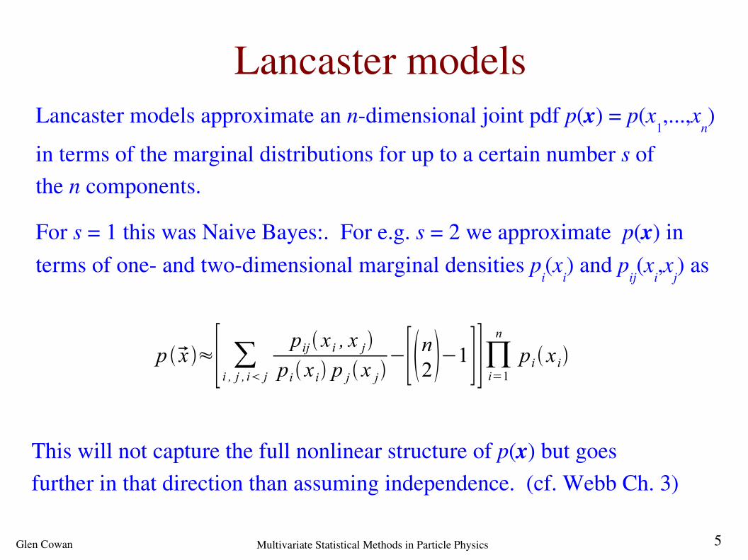
Lancaster modelsLancaster models approximate an ndimensional joint pdf p(x) = p(x

1,...,x

n)

in terms of the marginal distributions for up to a certain number s ofthe n components.

For s = 1 this was Naive Bayes:. For e.g. s = 2 we approximate p(x) in terms of one and twodimensional marginal densities p

i(x

i) and p

ij(x

i,x

j) as

p x ≈[ ∑i , j , i j pij x i , x jpi x i p j x j

−[n2−1]]∏i=1n

pi x i

This will not capture the full nonlinear structure of p(x) but goesfurther in that direction than assuming independence. (cf. Webb Ch. 3)


Parametric density estimationIf we have a parametric function for one or both of the densities,

p x ;1 , ,m

then we can estimate the parameters using the training data with e.g. the method of maximum likelihood, i.e., choose the parameterestimates to be the values that maximize the likelihood function:

L 1 , ,m=∏i=1

N

p x i ;1 , ,m

Product over all training events (assumes events statistically independent, not strictly true if we have multiple candidate “events” per collision event).

Finally simply take

p x ;1 , ,m

p x= p x ; 1 , , m

1 , , m

Function evaluation generally fast,storage requirements low.


Parametric density estimation (2)

Even if a full parametric model is not available, p(x) may (approximately)factorize into a parametric part for a subset of the variables:

p x1 , , xn= p x1 , , x s ;1 , ,mq x s1 , , xn

so we can mix parametric and nonparametric methods.

The number of parameters in a reasonable model is usually much smaller than the corresponding number of degrees of freedom in nonparametric methods, so a parametric estimate of the pdf will have higher statistical accuracy for a given amount of training data. Trade off:

few parameters: model not flexible and may not describe data,but parameters accurately determined.

many parameters: model flexible enough to describe the true pdf,but parameter estimates have large statistical errors.


HistogramsStart by considering onedimensional case, goal is to estimate pdf p(x)of continuous r.v. x.

Simplest nonparametric estimate of p(x) is a histogram:

Bishop Section 2.5

p x =ni

N x i for x in bin i

ni

xi

x

N total entries


Histograms (2)

Small bin width: estimate is very spiky, structure not really part of underlying distribution.

Medium bin width: best

Large bin width: too smooth and thus fails to capture e.g. bimodalcharacter of parent distribution

Bishop Section 2.5


Histograms (3)Advantages: once histogram computed, the data can be discarded.

Disadvantage: discontinuities at bin edges, scaling with dimensionality.

In general we can do much better than histograms, but they stillshow important features common to many methods:

To estimate pdf at x, = (x1, ..., x

D) we should count the number of

events in some local neighbourhood near x (requires definition of “local”, i.e., a distance measure, e.g., Euclidian).

The bin width x plays the role of a smoothing parameter definingthe size of the local neighbourhood. If it is too large, local structureis washed out; too small, and the estimate is subject to statistical fluctuations.


The curse of dimensionalityThe difficulty in determining the density in a highdimensional histogramis an example of the “curse of dimensionality” (Bellman, 1961).

The number of cells in a Ddimensional histogram grows exponentially.


Counting events in a local volumeConsider a small volume V centred about x = (x

1, ..., x

D).

This is in contrast to the histogram where the bin edges were fixed.

Suppose from N total events we find K in V.

p x = KN V

Take as estimate for p(x)

Two approaches:

Fix V and determine K from the data

Fix K and determine V from the data


Kernels

E.g. take V to be hypercube centered at the x where we want p(x).

k u=1for∣ui∣1/2 and 0 otherwise, i = 1, ..., DDefinei.e., the function is nonzero inside a unit hypercube centred about x and zero outside.

k(u) is an example of a kernel function (here called a Parzen window).


Kernel density estimators

Estimate p(x) using: p x = 1

N hD∑i=1

N

k x−x ih where we used V = hD for the volume of the hypercube.

Thus the estimate at x is the obtained from the sum of N hypercubes,one centred about each of the data points x

i.

This is an example of a kernel density estimator (KDE or Parzen estimator).

x where we want estimate

x of ith training event

side of hypercube


Gaussian KDEThe Parzen window KDE has discontinuities at the edges of thehypercubes; we can avoid these with a smoother kernel functione.g., Gaussian:

p x= 1N∑i=1

N1

2h21/2exp−∥x−x i∥

2

2h2 That is, to estimate p(x):

Place a Gaussian of standard deviation h centred about each training data point;

At a given x, add up the contribution from all the Gaussians anddivide by N.


Gaussian KDE, choice of h

Bishop Section 2.5

The Gaussian KDE shows the samebasic issues as did the histogram:


KDE – generalWe can choose any kernel function k(u) as long as it satisfies

k u0,

∫ k ud u=1

Advantage of KDE: essentially no training!To get p(x) simply compute the required sum of terms.

Disadvantages: A single function evaluation of p(x) requires carrying out the sum over all events, and the entire data set must be stored.


Expectation value of To see role of kernel, compute expectation value of

E [ p x ]= 1

N hD∑i=1

N

E [k x−x ih ]= 1

hDE [k x−x ih ]

= 1

hD∫ k x−x 'h p x ' d x '

Expectation value of the estimator is the convolution ofthe true density p(x) with the kernel function.

p x

For h 0 the kernel becomes a delta function, and E [ p x ]approaches the true density (zero bias). But for finite N the variance becomes infinite.V [ p x ]

p x p x


Choice of h using mean squared errorSuppose we knew the true p(x) (or had a reference standard). We can compute the Mean Squared Error (MSE) of our estimator:

MSE [ p x ]=E [ p x − p x 2]

=E [ p x − p x ] 2E [ p x − p x 2 ]

bias squared variance

We could e.g. choose h so that it minimizes the integral of the MSEover x (or maybe in some region of interest):

∫MSE [ p x ] d x

If both the kernel and p(x) are a Gaussian, this gives h= 43 1/5

N−1/5


Adaptive KDEIn the simplest form of KDE the smoothing parameter h is a constant.

In regions high density (lots of events) we want small h so as to not wash out structure.

In regions of low density, small h would lead to statistical fluctuationsin the estimate (structure not present in parent distribution).

So we may want to allow the size of the local neighbourhood overwhich we average to vary depending on the local density.

In sample point adaptive KDE the bandwidth becomes a function of p(x):

h=h0

p x


KDE boundary issuesSome components of x may have finite limits. But if we use e.g. a Gaussian kernel, then some of the probability “spills out” of the allowed range.

The probability inside the range is therefore underestimated.

One solution is to renormalize the kernel so that its integral insidethe allowed range is equal to unity.

Another option is to “mirror” the distribution about the boundary.The events from outside spilling in compensate those spilling out.


Knearest neighbour method

Bishop Section 2.5

Instead of fixing V, consider a fixed number of events Kand find the appropriate V such that it just contains K events.

The density estimate is then simply p x = KN V

K plays role of smoothing parameter.Large K means lower statistical error in the estimate of the density,e.g., K=100 gives 10% accuracy. But large K means you need a biggervolume, estimate is less local.

Estimate of p(x) is not a true pdf – integral over entire space diverges.


Knearest neighbour methodExample from TMVA manual – here the algorithm is used directlyas a classifier. The event type is assigned based on majorityvote within the volume.


KNN algorithms rely on a metric in the input variable spaceto define the volume.

If there is a great difference in the ranges spanned by some of thevariables, then they are implicitly given different weights.

Typically scale the input variables so as to give approximatelyequal distances between relevant features. Try e.g.

Feature normalization

x '= x−xminxmax−xmin

0x '1Linear scaling in unit range:

x '= x−

Standardization: (zero mean, unit variance)


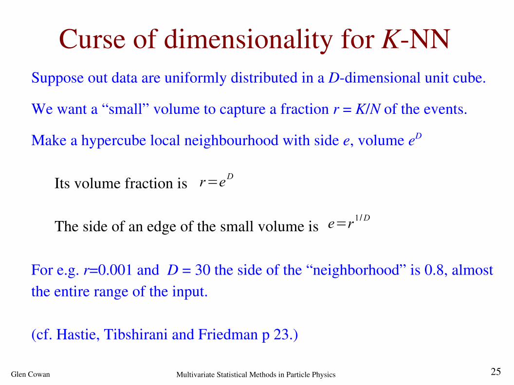
Curse of dimensionality for KNN Suppose out data are uniformly distributed in a Ddimensional unit cube.

We want a “small” volume to capture a fraction r = K/N of the events.

Make a hypercube local neighbourhood with side e, volume eD

Its volume fraction is

The side of an edge of the small volume is

For e.g. r=0.001 and D = 30 the side of the “neighborhood” is 0.8, almost the entire range of the input.

(cf. Hastie, Tibshirani and Friedman p 23.)

r=eD

e=r1/D


Lecture 3 summaryMany important classification methods rely on obtaining estimates ofthe multivariate probability densities. We can use e.g.

Histograms

Kernel density estimation (parzen window)

Knearest neighbour

Both KDE and KNN methods require the entire data set to beretained, and all become problematic in higher dimensions.

But if the pdfs are not too nonlinear, the density estimation can be done in lower dimension (Naive Bayes, Lancaster models).

Documents

Advanced statistical methods for data analysis – Lecture 3cowan/mva/cowan_mva_3.pdf · Glen Cowan Multivariate Statistical Methods in Particle Physics 1 Advanced statistical methods