Advanced Networking

Lecture for September 17

X.25, Frame and ATM

Many of these figures were adapted from Tanenbaum (Computer Networks) and from Forouzan (Data Communications and Networking)

Shared medium drawbacks

• Shared-medium networks do not scale– Simple hub sends incoming frames to all output

ports – (a layer 1 hub)– As more nodes are added, congestion becomes

a problem >> it’s a shared medium

A B

C

DE

F

G

10Base2

10BaseT

Layer 2 Switching

• Layer 2 switch is used to interconnect LAN segments– Usually Ethernet

• Types of layer 2 switches– Simple Bridge

– Multiport Bridge

– Transparent Bridge

– Remote Bridge

– Possibly others??

Hub and Spoke (cont)

• Filtering alleviates this problem– Why not just send the frames to the destination port and

not the others?– This requires processing the destination fields in the

frame

• Drawbacks:– Requires the switching fabric to be much faster than

before• 10 users all transmitting at 100Mbps >>> 1Gbps

– Hub must be able to “Learn” the proper destination• i.e. How does the hub know to selectively forward frames?

Bridges

• Bridges forward at Layer2 based on destination MAC address in Ethernet frame– When Ethernet frame comes in, sent out only

on port corresponding to MAC address in table

Port # MAC address

0 2b:6:8:f:1e:5b

1 f:1e:5b:2b:6:8

2 2b:6:8:f:1e:51

Problem: How is this table built???

Learning Bridges

• Bridges are Hubs that filter and forward selected layer 2 frames.

A B

C

DE

F

GH I

J

KL

M

N

Bridging Switch

Learning Bridge (cont)

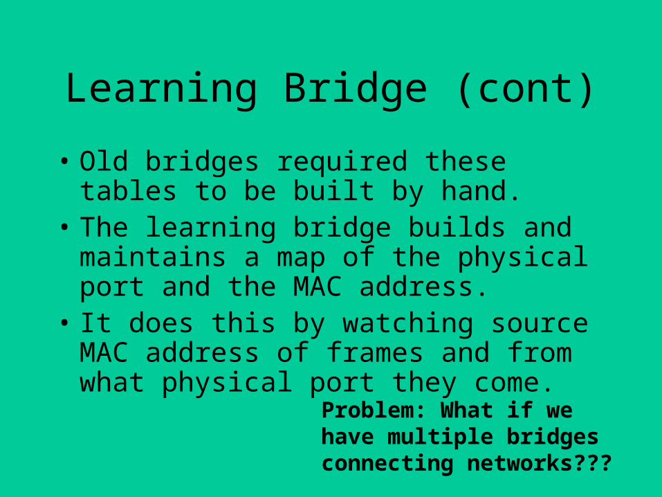
• Old bridges required these tables to be built by hand.

• The learning bridge builds and maintains a map of the physical port and the MAC address.

• It does this by watching source MAC address of frames and from what physical port they come. Problem: What if we have

multiple bridges connecting networks???

Spanning Tree Bridges

Two parallel transparent bridges.

These can create multiple copies of the frame. Can also cause forwarding loops.

Spanning tree (cont)

• Often multiple bridges are used for redundancy. • Spanning tree algorithm is used to eliminate

forwarding loops and multiple copies of frames.• Routes and bridges with lower numbers become

primary elements of the spanning tree.• Other routes and bridges are used in the event of a

failure• Exact algorithm is detailed but straightforward.• Algorithm also used at layer 3 for multicast IP and

other applications.

Spanning Tree Bridges (2)

(a) Interconnected LANs. (b) A spanning tree covering the LANs. The dotted lines are not part of the spanning tree.

Bridges from 802.x to 802.y

Operation of a LAN bridge from 802.11 to 802.3.

MAC layers are different for .11 and .3, LLC the same

Bridges from 802.x to 802.y (2)

The IEEE 802 frame formats.

Remote Bridges

• Remote bridges can be used to interconnect distant LANs.

Repeaters, Hubs, Bridges, Switches, Routers and Gateways

(a) Which device is in which layer.(b) Frames, packets, and headers.

Figure 17-1

X.25

X.25

• Was the first popular packet switched network• Allowed for the setup of data connections at

speeds between 300bps to about 56kbps.• Uses the “Virtual Circuit” concept.

– Connection oriented packet switch.

• Still used for low bandwidth transactions – credit cards / Point-of-Sale (POS) transactions.

– Telemetry networks.

Figure 17-2

X.25 Layers in Relation to the OSI Layers

Figure 17-3

Format of a Frame

Figure 17-6

Frame Layer and Packet Layer Domains

Figure 17-7

Virtual Circuits in X.25

Virtual circuits allow “meshy” network with fewer physical links.

Figure 17-8

LCNs in X.25

LCN: Logical Channel Number, identifies the VC at different sections of the network.

Figure 17-10

PLP Packet Format

Note the LCN is in the Layer 3 portion of the protocol.

GFI: General Format Identifier-- defines which device should acknowledge the packet

PTI: Packet Type Identifier – The type of packet

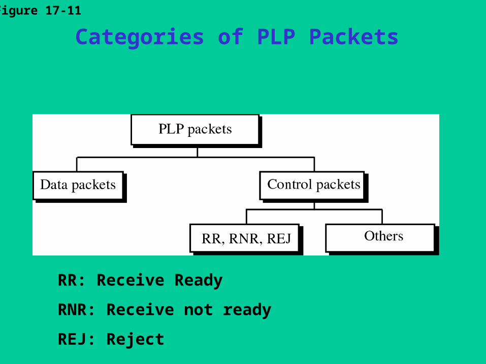
Figure 17-11

Categories of PLP Packets

RR: Receive Ready

RNR: Receive not ready

REJ: Reject

Figure 17-12

Data Packets in the PLP Layer

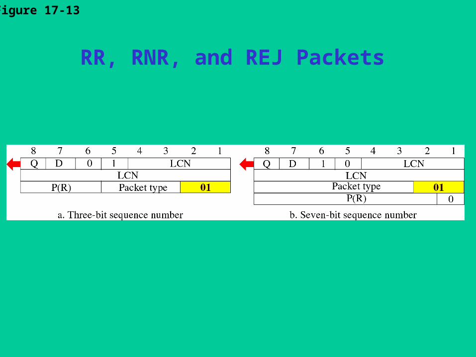
Figure 17-13

RR, RNR, and REJ Packets

Figure 17-14

Other Control Packets

Figure 17-15

Control Packet Formats

Figure 17-17

Triple-X Protocols

Key points on X.25

• Was developed as a packet switching protocol.• Standard includes Layer 1,2,3• Incorporates SVCs and PVCs• Limited in bandwidth• Not optimized for high quality links

– Too much error checking for “good” networks

• Not optimized for TCP / IP transport– Already has PLP defined at Layer 3

Chapter 18

FrameRelay

Figure 18-1

Frame Relay versus Pure Mesh T-Line Network

Figure 18-2

Fixed-Rate versus Bursty Data

Figure 18-3

X.25 Traffic

Figure 18-4

Frame Relay Traffic

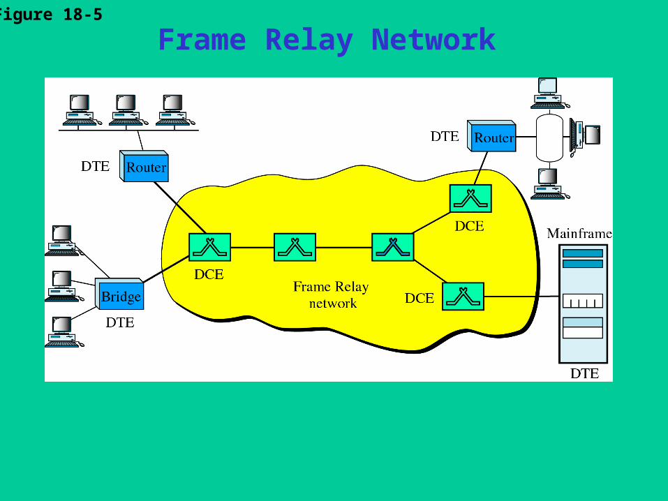
Figure 18-5

Frame Relay Network

Figure 18-6

DLCIs: Data Link Connection Identifier

Figure 18-7

PVC DLCIs

Figure 18-8

SVC Setup and Release

Figure 18-9

SVC DLCIs

Figure 18-10

DLCIs Inside a Network

Note that the overall connection is a mixture of different interfaces and DLCIs

This allows DLCIs to be re-used on different interfaces

Figure 18-11

Frame Relay Switch

Figure 18-12

Frame Relay Layers

Figure 18-13

Comparing Layers in Frame Relay and X.25

Figure 18-14

Frame Relay Frame

Figure 18-15

BECN

BECN assumes the source can reduce congestion by slowing down the transmission of data.

Figure 18-16

FECN

FECN notifies the receiver that congestion is occurring. It can then be more patient and not request so much data.

Figure 18-17

Four Cases of Congestion

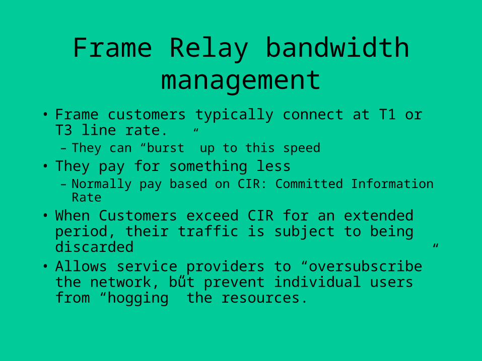
Frame Relay bandwidth management

• Frame customers typically connect at T1 or T3 line rate. – They can “burst” up to this speed

• They pay for something less– Normally pay based on CIR: Committed Information Rate

• When Customers exceed CIR for an extended period, their traffic is subject to being discarded

• Allows service providers to “oversubscribe” the network, but prevent individual users from “hogging” the resources.

Figure 18-18

LeakyBucket

Figure 18-19

A Switch Controlling the Output Rate

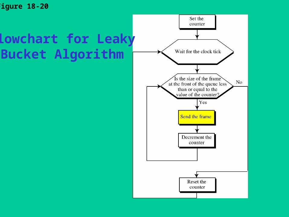
Figure 18-20

Flowchart for LeakyBucket Algorithm

Figure 18-21

Example of Leaky Bucket Algorithm

Figure 18-22

Relationship between TrafficControl Attributes

Figure 18-23

User Rate in Relation to Bc and Bc + Be

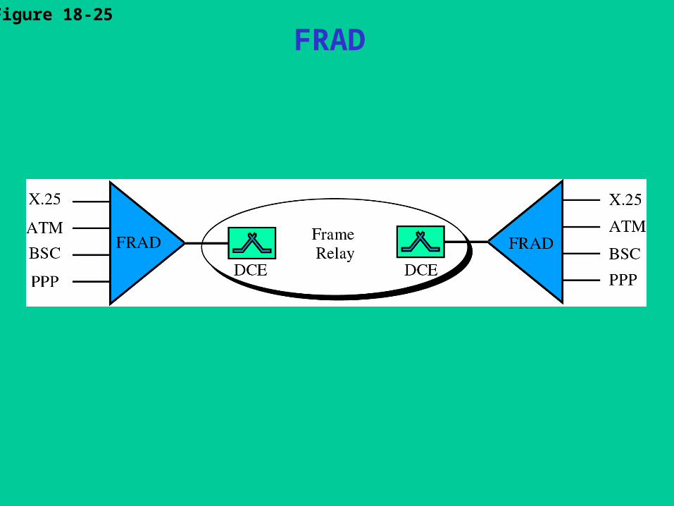
Figure 18-25

FRAD

Chapter 19

ATM

ATM in context

• Development of ATM began prior to the WWW and TCP/IP explosion- early nineties.

• There was a desire for a packet switched protocol that was faster than X.25 and Frame and could support multiple classes of service– Video, Voice, Data

• ATM was selected as the technology of choice for BISDN– The plan was to allow “fast” phone calls all over the

place. These could support differing levels of bandwidth and QoS.

Figure 19-1

Multiplexing Using Different Packet Sizes

53 byte “cell” allowed for higher levels of QoS with minimal cell-tax – the ratio of overhead to payload in the cell.

Figure 19-2

Multiplexing Using Cells

Figure 19-3

ATM Multiplexing

Figure 19-4

Architecture of an ATM Network

UNI – User to Network Interface

NNI – Network to Network Interface

Figure 19-5

TP, VPs, and VCs

TP: Transmission path – link between two switches

VP: Virtual Path – Contains several VCs

VC: Virtual Circuit

Figure 19-6

Example of VPs and VCs

VPs originally conceived to simplify management of VC bundles

Figure 19-7

Connection Identifiers

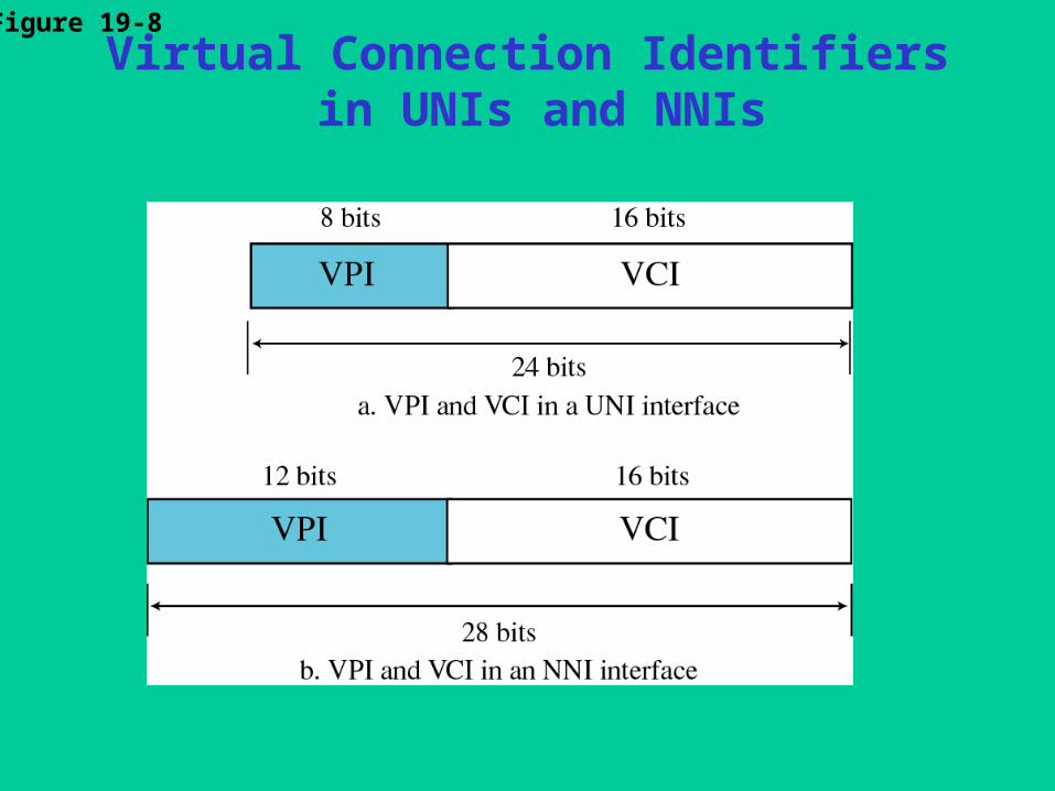
Figure 19-8

Virtual Connection Identifiers in UNIs and NNIs

Figure 19-9

An ATM Cell

Figure 19-10

SVCSetup

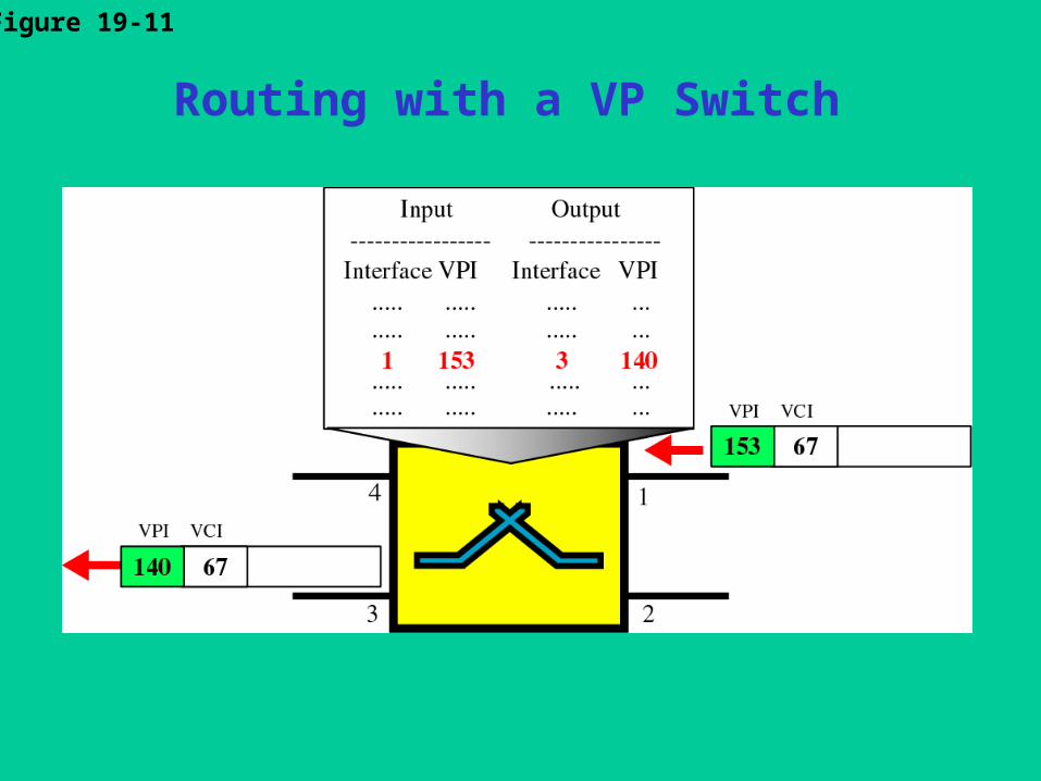
Figure 19-11

Routing with a VP Switch

Figure 19-12

A Conceptual View of a VP Switch

In theory, a VP switch is simpler because it just switches based on the VPI. Fewer entries to be maintained.

Figure 19-13

Routing with a VPC Switch

Figure 19-14

A Conceptual View of a VPC Switch

Figure 19-15

Crossbar Switch

Figure 19-16Knockout Switch

Output queuing reduces lost cells.

Introduces some jitter.

Figure 19-17 A Banyan Switch

Self routing switch, minimizes control hardware required.

A multi-stage switch

Figure 19-18-Part I

Example of Routing in a Banyan Switch (a)

Figure 19-18-Part II

Example of Routing in a Banyan Switch (b)

Figure 19-19

Batcher-Banyan Switch

Cells are reordered at input port so they don’t block each other as they go through the fabric

Figure 19-20

ATM Layers

Figure 19-21

ATM Layers in End-Point Devices and Switches

Figure 19-27

ATM Layer

ATM Adaption Layers

• These allow other protocols to mapped into cells.• AAL1: Good for Constant Bit Rate (CBR)• AAL2

– Variable Bit Rate Services – Particularly Video

• AAL3/4• AAL5

– Ethernet and IP – Data oriented protocols

• Lots of references available on these

Figure 19-28ATM Header

Figure 19-29

PT Fields

Figure 19-30

Service Classes

QoS

• Constant Bit Rate (CBR) used for carrying DS1 and DS3 or other traffic requiring a constant guaranteed QoS

• VBR (Real Time and Non Real Time) used for data that is bursty but need QoS– Especially for Video

• UBR/ABR lower QoS for Data similar to Frame Relay level of QoS

Figure 19-31

Service Classes and Capacity of Network

Figure 19-32

QoS

Lots of parameters for QoS. Homework: Go look these up and also understand the concept of CAC.

Figure 19-33

ATM WAN

Figure 19-34

Ethernet Switch and ATM Switch

ATM hasn’t really taken hold in the Enterprise. Much more expensive than Ethernet switches.

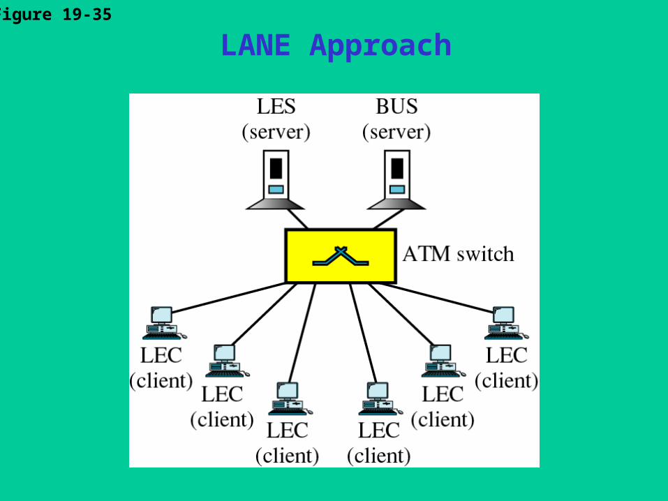
Figure 19-35

LANE Approach