Embed Size (px)
Citation preview

RealTide Project – Grant Agreement No 727689
D3.1 Generalised tide-to-wire model
This Document is the property of RealTide Consortium
European Commission
H2020 Programme for Research & Innovation
Advanced monitoring, simulation and control of tidal
devices in unsteady, highly turbulent realistic tide
environments

RealTide Project – Grant Agreement No 727689
D3.1 Generalised tide-to-wire model
This Document is the property of RealTide Consortium
Grant Agreement number: 727689
Project Acronym: RealTide
Project Title: Advanced monitoring, simulation and control of tidal devices in
unsteady, highly turbulent realistic tide environments
Deliverable Number (D3.1)
Generalised tide-to-wire-model
WP 3
Realistic Simulation of Tidal Turbines
WP Leader: UEDIN
Dissemination level: Public
Summary:
The report D3.1 details the theory, for the mechanical and electrical part, used for the development of the tide-to-wire
model in Python code. Some application cases are also presented for the validation of the tool.
Objectives:
The objective of the task T3.1 is to develop a time dependant tide-to-wire model using blade element momentum
theory (BEMT) to calculate the torque and thrust on a tidal turbine. From an input of the tidal conditions, the tool is
also able to predict the power output in terms of electrical parameters and accounts for realistic tidal conditions such
as turbulent and unsteady flow.

RealTide Project – Grant Agreement No 727689
D3.1 Literature Review - Evaluation of force on tidal blades
Page | 1
This Document is the property of RealTide Consortium
Table of ContentsTable of ContentsTable of ContentsTable of Contents
1. Introduction ..................................................................................................................................... 7
1.1 Abbreviations & Definitions .................................................................................................... 7
1.2 References ............................................................................................................................... 8
1.3 Distribution List ..................................................................................................................... 11
2 Blade Element Momentum Theory ............................................................................................... 12
2.1 Blade Element Momentum Theory ....................................................................................... 12
2.2 Solution to the BEMT equations............................................................................................ 13
2.3 BEMT: SWOT analysis ............................................................................................................ 14
3 Improvements to BEMT ................................................................................................................ 17
3.1 Losses at blade tip and root .................................................................................................. 17
3.2 High Induction Factor ............................................................................................................ 18
3.3 Root finding algorithms ......................................................................................................... 19
3.4 Wake models ......................................................................................................................... 19
3.5 Dynamic Stall model .............................................................................................................. 20
3.6 Single-variable optimization .................................................................................................. 21
3.7 Turbulence Model ................................................................................................................. 21
3.8 Loads on Tidal Turbines ......................................................................................................... 22
3.9 Optimization Algorithms ....................................................................................................... 22
4 Existing BEMT Tools ....................................................................................................................... 24
4.1 Software Packages ................................................................................................................. 24
4.2 Input ...................................................................................................................................... 25
4.3 BEMT Improvements ............................................................................................................. 30
4.4 Other features ....................................................................................................................... 31
5 Program Architecture .................................................................................................................... 32
5.1 Iterative loops ........................................................................................................................ 32
5.2 Blade Geometry Data ............................................................................................................ 36
5.3 Operating Conditions ............................................................................................................ 36
5.4 Python Libraries ..................................................................................................................... 37
5.5 Python Scripts ........................................................................................................................ 38
5.6 File Formats ........................................................................................................................... 39
6 BEMT Computations ...................................................................................................................... 40

RealTide Project – Grant Agreement No 727689
D3.1 Generalised tide-to-wire model
Page | 2
This Document is the property of RealTide Consortium
6.1 Thrust and Torque of Turbine ............................................................................................... 41
6.2 Shear Force & Bending Moment Distribution ....................................................................... 44
6.3 Dynamic Stall Module ............................................................................................................ 46
7 Pre processor – User Interface ...................................................................................................... 51
7.1 Geometry of the tidal turbine ............................................................................................... 52
7.2 User input of Velocity Profile ................................................................................................ 55
7.3 Definition of Rotation Speed ................................................................................................. 58
7.4 Selection of BEMT Improvement modules ............................................................................ 58
8 Post Processing .............................................................................................................................. 59
8.1 Independent variables ........................................................................................................... 61
8.2 Relational hierarchy............................................................................................................... 61
9 Validation Case Studies ................................................................................................................. 64
9.1 Bahaj ...................................................................................................................................... 64
9.2 Sabella D10 ............................................................................................................................ 67
9.3 Hobit ...................................................................................................................................... 70
9.4 Dynamic Stall Validation ........................................................................................................ 74
10 Electrical Modelling and control of grid connected tidal current conversions systems ........... 76
10.1 Review of electrical modelling for tidal current conversion systems ................................... 76
10.2 Methodology for electrical and control modelling for tidal current conversion systems .... 83
10.3 Condition Monitoring Based on Model Based Estimation .................................................... 89
10.4 Results from the tidal current conversion system ................................................................ 94
11 Coupled BEMT and electrical model ......................................................................................... 99
12 Conclusion ............................................................................................................................... 103
Appendix A: USER GUIDE..................................................................................................................... 104
OPERATING INSTRUCTIONS FOR USE OF BEMT tool ....................................................................... 104
OPERATING INSTRUCTIONS FOR POSTPROCESSING ....................................................................... 109
Appendix B: Paper EWTEC Conference ............................................................................................... 111

RealTide Project – Grant Agreement No 727689
D3.1 Generalised tide-to-wire model
Page | 3
This Document is the property of RealTide Consortium
List of FiguresList of FiguresList of FiguresList of Figures
FIGURE 1: TIDE-TO-WIRE MODEL FOR A GENERALISED TIDAL TURBINE ..................................................................................... 7
FIGURE 2: ANNULAR REGION TRACED OUT BY A BLADE ELEMENT [3] .................................................................................... 12
FIGURE 3: AXIAL STREAM AROUND A WIND TURBINE [2] .................................................................................................... 13
FIGURE 4: BLADE SECTION DIAGRAM SHOWING FORCE COMPONENTS ................................................................................... 14
FIGURE 5: BLADE SECTION DIAGRAM SHOWING VELOCITY COMPONENTS [3] .......................................................................... 14
FIGURE 6: SWOT ANALYSIS OF BEMT ........................................................................................................................... 16
FIGURE 7: CONVENTIONAL STAGES OF DYNAMIC STALL [22] [24] ....................................................................................... 21
FIGURE 8: PROGRAM ARCHITECTURE FLOWCHART ............................................................................................................ 35
FIGURE 9: VELOCITY VECTOR DIAGRAM FOR BLADE ELEMENT (TOP-VIEW) .............................................................................. 42
FIGURE 10: FORCE VECTOR DIAGRAM FOR BLADE ELEMENT (TOP-VIEW) ................................................................................ 42
FIGURE 11: FRONT VIEW OF BLADE SHOWING ELEMENTAL FORCES ....................................................................................... 43
FIGURE 12: DISTRIBUTION OF FORCES, SHEAR FORCE AND BENDING MOMENT ALONG BLADE LENGTH ......................................... 45
FIGURE 13: TRAILING EDGE SEPARATION POINT AS PER KIRCHOFF THEORY [1] ........................................................................ 47
FIGURE 14: GRAPHICAL USER INTERFACE FOR THE PYTHON CODE ........................................................................................ 51
FIGURE 15: WINDOW FOR ENTRY OF GEOMETRICAL DATA .................................................................................................. 52
FIGURE 16: WINDOW FOR ENTRY OF LIFT AND DRAG COEFFICIENTS ..................................................................................... 54
FIGURE 17 : INFORMATION ABOUT BLADE ELEMENTS AND BLADE SEGMENTS .......................................................................... 54
FIGURE 18: VITERNA EXTRAPOLATED LIFT AND DRAG COEFFICIENTS ..................................................................................... 55
FIGURE 19 : CONVENTIONAL EXPERIMENTAL SET-UP FOR PERFORMANCE EVALUATION OF TIDAL TURBINES ................................... 56
FIGURE 20: USER INPUT OF VELOCITY PARAMETERS (CONSTANT VELOCITY) ............................................................................ 57
FIGURE 21: VELOCITY INPUT AS PER NI603 .................................................................................................................... 57
FIGURE 22: HIERARCHY OF ‘RESULTS’ VARIABLE ............................................................................................................... 60
FIGURE 23: RELATIONAL MAPPING FOR OUTPUT VARIABLES ................................................................................................ 62
FIGURE 24: POSTPROCESSING GUI WINDOW .................................................................................................................. 63
FIGURE 25: POSTPROCESSING OUTPUT OPTIONS .............................................................................................................. 63
FIGURE 26: EXPERIMENTAL SET-UP FOR BAHAJ MODEL ...................................................................................................... 65
FIGURE 27: COMPARISON OF CT, CQ, AND CP - BAHAJ VALIDATION ................................................................................... 67
FIGURE 28: SABELLA D10 TURBINE BEFORE OFFSHORE INSTALLATION .................................................................................. 68
FIGURE 29: COMPARISON OF CT, CQ, CP - SABELLA D10 VALIDATION ................................................................................ 69
FIGURE 30: D10 VALIDATION WITH NO TIP & HUB LOSSES ................................................................................................. 70
FIGURE 31: BLADE SHAPE FOR HOBIT ........................................................................................................................... 71
FIGURE 32: COMPARISON OF CT - HOBIT VALIDATION ...................................................................................................... 73
FIGURE 33: COMPARISON OF CP - HOBIT VALIDATION ...................................................................................................... 73

RealTide Project – Grant Agreement No 727689
D3.1 Generalised tide-to-wire model
Page | 4
This Document is the property of RealTide Consortium
FIGURE 34: DYNAMIC STALL VALIDATION -S814, RED. FREQ. = 0.090 ................................................................................ 74
FIGURE 35: S814 VALIDATION - LOW FREQUENCY ............................................................................................................ 75
FIGURE 36: S814 VALIDATION - MEDIUM FREQUENCY ...................................................................................................... 75
FIGURE 37: BLOCK DIAGRAMS OF SINGLE TCCS. A. SCIG AND PMSG OPTIONS WITH LONG DISTANCE CONTROLS. B. SCIG AND PMSG
OPTIONS WITH BACK-TO-BACK CONVERTERS IN THE NACELLE [43]. .............................................................................. 77
FIGURE 38: BLOCK DIAGRAM OF THE SINGLE TCCS WITH LONG DISTANCE CONTROLS AND THE ASSOCIATED CONTROL BLOCKS [43]. . 77
FIGURE 39: SCHEMATIC DIAGRAM OF THE GRID CONNECTED DFIG AS PRESENTED IN [49]. ....................................................... 79
FIGURE 40: SCHEMATIC DIAGRAM OF THE PMSG TIDAL CURRENT SYSTEM [51]. .................................................................... 80
FIGURE 41: TIDE-TO-GRID MODEL DEVELOPED IN MATLAB/SIMULINK USED FOR GENERATOR COMPARISON [55]. ...................... 82
FIGURE 42: (A) VARIABLE FREQUENCY FROM THE NACELLE COLLECTION ARRANGEMENTS. (B) FIXED FREQUENCY FROM THE NACELLE
ARRANGEMENTS [57]. ....................................................................................................................................... 82
FIGURE 43: (A) DC OUTPUT FROM THE NACELLE ARRANGEMENTS. (B) PREFERRED POWER COLLECTION SOLUTIONS FOR TIDAL CURRENT
ARRAYS [57]. ................................................................................................................................................... 83
FIGURE 44: BLOCK DIAGRAM OF THE RESOURCE-TO-GRID MODEL DEVELOPED. ....................................................................... 84
FIGURE 45: BLOCK DIAGRAM OF THE ZDC SVM GENERATOR CONTROLLER [56]. ................................................................... 85
FIGURE 46: TORQUE SPEED CURVES FOR DIFFERENT TIDAL CURRENT VELOCITIES FOR A SIMULATION MODEL OF XMED TURBINE. THE
PEAK MECHANICAL TORQUE IS IDENTIFIED (BLUE DOTS) AND A CURVE IS FITTED BASED ON EQ.4 WHICH FORMS THE MPPC. ... 86
FIGURE 47: SPEED CONTROLLER BLOCK DIAGRAM AS MODELLED FOR THE RESOURCE-TO-GRID TCCS TOOL. ................................. 87
FIGURE 48: BLOCK DIAGRAM OF THE DC LINK MODEL IMPLEMENTED IN SIMULINK AND OPENMODELICA. ................................... 87
FIGURE 49: VOC CONTROLLER AS IMPLEMENTED IN THE RESOURCE-TO-GRID TCCS. ............................................................... 88
FIGURE 50: SCHEMATIC DESCRIPTION OF THE RESIDUAL GENERATOR .................................................................................... 90
FIGURE 51: DYNAMICAL BEHAVIOUR MODEL ................................................................................................................... 91
FIGURE 52: VARIABLE SPEED AC MOTOR DIAGRAM. ......................................................................................................... 92
FIGURE 53: DC-LINK VOLTAGE �� IN THE PRESENCE OF DIFFERENT FAULTS (SAMPLING FREQUENCY 2 KHZ) ................................ 92
FIGURE 54: VARIANCE OF DC-LINK VOLTAGE �� FOR DIFFERENT FAULTS ............................................................................. 92
FIGURE 55: STATOR CURRENT VECTOR TRAJECTORIES. ....................................................................................................... 93
FIGURE 56: RESULTS FROM THE SIMULATED TCCS. (A) MECHANICAL TORQUE INPUT. (B) REFERENCE AND MEASURED ROTATIONAL
SPEED. (C) MECHANICAL, GENERATOR AND GRID POWER. .......................................................................................... 95
FIGURE 57: GENERATOR STATOR VOLTAGE AND CURRENT. (A) PHASE A STATOR CURRENT. (B) PHASE A STATOR CURRENT ZOOMED AT
40S SIMULATION TIME. (C) PHASE A STATOR VOLTAGE. (D) PHASE A STATOR VOLTAGE ZOOMED AT 40S SIMULATION TIME. .. 96
FIGURE 58: RESULTS FROM THE SIMULATED TCCS WITH VARIABLE INPUT. (A) MECHANICAL TORQUE INPUT. (B) REFERENCE AND
MEASURED ROTATIONAL SPEED. (C) MECHANICAL, GENERATOR AND GRID POWER. ......................................................... 97
FIGURE 59: GENERATOR STATOR VOLTAGE AND CURRENT FOR VARIABLE MECHANICAL TORQUE INPUT. (A) PHASE A STATOR CURRENT.
(B) PHASE A STATOR CURRENT ZOOMED AT 40S SIMULATION TIME. (C) PHASE A STATOR VOLTAGE. (D) PHASE A STATOR
VOLTAGE ZOOMED AT 40S SIMULATION TIME. ......................................................................................................... 98
FIGURE 60: PROCESS TO GENERATE THE FMU OF THE ELECTRICAL MODEL DEVELOPED IN OPENMODELICA AND LOAD IT IN PYTHON . 99
FIGURE 61: COUPLING OF BEMT CODE AND FMU. EXCHANGE OF INFORMATION AT REGULAR INTERVALS. ............................... 100
FIGURE 62: COMPARISON OF EXPERIMENTAL AND SIMULATED RESULTS USING A COUPLED BEMT AND ELECTRICAL MODEL IN PYTHON.
(A) TIDAL CURRENT VELOCITY INPUT. (B) MECHANICAL TORQUE. (C) TURBINE ROTATIONAL SPEED. .................................. 101
FIGURE 63: RESULTS FROM THE OPERATION OF THE COUPLED BEMT AND ELECTRICAL MODEL WITH THE MPPT SYSTEM ENABLED. (A)
TIDAL CURRENT VELOCITY FROM MEASURED EXPERIMENT. (B) MECHANICAL TORQUE OF THE TIDAL TURBINE. (C) ROTATIONAL

RealTide Project – Grant Agreement No 727689
D3.1 Generalised tide-to-wire model
Page | 5
This Document is the property of RealTide Consortium
SPEED OF THE TIDAL CURRENT TURBINE. (D) POWER AT DIFFERENT LEVELS OF THE RESOURCE-TO-GRID SYSTEM. (E)
HYDRODYNAMIC COEFFICIENT OF THE TURBINE. (F) THRUST FORCE ON THE TURBINE. .................................................... 102
FIGURE 64: COUPLING OF BEMT TOOL WITHIN REALTIDE PROJECT ................................................................................... 103
FIGURE 65: SCHEMATIC DIAGRAM OF TIDE-TO-WIRE MODEL ............................................................................................. 111

RealTide Project – Grant Agreement No 727689
D3.1 Generalised tide-to-wire model
Page | 6
This Document is the property of RealTide Consortium
List of List of List of List of TTTTablesablesablesables TABLE 1: INPUT VELOCITY PROFILE FOR VARIOUS SOFTWARE PACKAGES ................................................................................. 26
TABLE 2: CAPABILITIES OF SOFTWARE PACKAGE W.R.T. INPUT VELOCITY PROFILE ..................................................................... 27
TABLE 3: COMPARISON OF LIFT-DRAG COEFFICIENT INPUT DATA .......................................................................................... 28
TABLE 4: ENVIRONMENTAL EFFECTS CONSIDERED WITHIN THE SOFTWARE PACKAGES ............................................................... 29
TABLE 5: RANGE OF TSR AS INPUT IN THE CODE ............................................................................................................... 29
TABLE 6: COMPARISON OF BASIC BEMT IMPROVEMENTS .................................................................................................. 30
TABLE 7: COMPARISON OF IMPROVEMENTS BASED ON DYNAMIC EFFECTS ............................................................................. 30
TABLE 8: DATAFRAME STRUCTURE FOR DIFFERENT BLADE ELEMENTS ON A SINGLE BLADE .......................................................... 36
TABLE 9: BLADE GEOMETRY – BAHAJ VALIDATION ............................................................................................................ 65
TABLE 10: BLADE SEGMENTS – BAHAJ VALIDATION ........................................................................................................... 66
TABLE 11: LIST OF OPERATING CONDITIONS – BAHAJ VALIDATION........................................................................................ 66
TABLE 12: LIST OF OPERATING CONDITIONS - SABELLA D10 VALIDATION.............................................................................. 68
TABLE 13: MAIN GEOMETRICAL PARAMETERS - HOBIT VALIDATION ..................................................................................... 71
TABLE 14: BLADE GEOMETRY – HOBIT VALIDATION .......................................................................................................... 71
TABLE 15: BLADE SEGMENTS – HOBIT VALIDATION ........................................................................................................... 72
TABLE 16: LIST OF OPERATING CONDITIONS - HOBIT VALIDATION ....................................................................................... 72
TABLE 17: ADVANTAGES AND DISADVANTAGES FOR DIFFERENT GENERATOR TYPES. TABLE ADAPTED FROM [55]. .......................... 80
TABLE 18: DESCRIPTION OF QUANTITIES OF THE DYNAMIC PMSG MODEL. ............................................................................ 85
TABLE 19. FAULT SYMPTOM TABLE FOR THE PWM CONVERTER AND STATOR WINDINGS .......................................................... 94

RealTide Project – Grant Agreement No 727689
D3.1 Generalised tide-to-wire model
Page | 7
This Document is the property of RealTide Consortium
1.1.1.1. INTRODUCTIONINTRODUCTIONINTRODUCTIONINTRODUCTION
The objective of the task T3.1 is to develop a time dependant tide-to-wire model using blade element
momentum theory (BEMT) to calculate the torque and thrust on a tidal turbine. From an input of the
tidal conditions, the tool is also able to predict the power output in terms of electrical parameters and
accounts for realistic tidal conditions such as turbulent and unsteady flow.
This document presents development performed by Bureau Veritas (BV) and University of Edinburgh
(UEDIN) to achieve this objective. The report starts by an explanation of the BEMT, the possible
improvements of the theory that have been implemented in the code and a review of existing tools
using BEMT. Then, the program architecture using Python code and equations used are fully detailed
in next sections. Pre and post processing strategy are also described. Some validation cases have been
used in order to confirm results of the tool, based on previous experiments or simulations. The
methodology for the electrical is fully explained as well as the condition monitoring based on model
based. Finally, the coupling between the BEMT model, developed by BV in python, and the electrical
Tidal Current Conversion System model developed by UEDIN is presented. The tide-to-wire model
integration in a Computational Fluid Dynamics solver will be performed in task T3.3.
In appendix, the user guide of the tool and an abstract submitted to EWTEC conference in 2019 are
presented.
Figure 1: Tide-to-wire model for a generalised tidal turbine
1.11.11.11.1 Abbreviations & DefinitionsAbbreviations & DefinitionsAbbreviations & DefinitionsAbbreviations & Definitions
BV Bureau Veritas
BV M&O Bureau Veritas Marine & Offshore
HO HydrOcean
UEDIN The University of Edinburgh
EO EnerOcean
SAB Sabella
1-T 1-Tech

RealTide Project – Grant Agreement No 727689
D3.1 Generalised tide-to-wire model
Page | 8
This Document is the property of RealTide Consortium
IFR Ifremer (Institut Français pour la Recherche et l’Exploitation de la Mer
ISSA Ingeteam Power Technology
GA Grant Agreement
PMP Project Management Plan
BEMT Blade Element Momentum Theory
CFD Computational Fluid Dynamics
TCCS Tidal Current Conversion System
1.21.21.21.2 ReferencesReferencesReferencesReferences
[1] G. T. Scarlett, B. Sellar, T. v. d. Bremer and I. M. Viola, “Unsteady hydrodynamics of a full-scale
tidal turbine operating in large wave conditions,” 2018.
[2] G. Ingram, “Wind Turbine Blade Analysis using the Blade Element Momentum Method,” Durham
University, 2011.
[3] G. T. Scarlett, T. v. d. Bremer, B. Sellar and I. M. Viola, “Unsteady hydrodynamics of full-scale tidal
turbine blades”.
[4] S. Hermant, “Development of a precise BEMT numerical model,” Marine Renewable Energies
Project, HydrOcean.
[5] P. Moriarty and A. Hansen, AeroDyn Theory Manual, National Renewable Energy Laboratory,
2005.
[6] I. Masters, J. Chapman, O. J.A.C and W. M.R, “Modelling high axial induction flows in tidal stream
turbines with a corrected blade element model,” Bilbao, 2010.
[7] DNV GL, Tidal Bladed Theory Manual, 2014.
[8] H. Glauert, “Aerodynamic Theory,” in Airplane Propellers, Springer, 1935.
[9] W. Z. Shen, R. Mikkelson, J. N. Sorenson and B. Christian, “Tip loss corrections for wind turbine
computations,” vol. 8, no. 4, 2005.
[10] M. Buhl, “A New Empirical Relationship between Thrust Coefficient and Induction Factor for the
Turbulent Mill State,” NREL, 2005.
[11] T. Burton, D. Sharpe, N. Jenkins and E. Bossanyi, Wind Energy Handbook, John Wiley & Sons Ltd..
[12] S. A. Ning, “A simple solution method for the blade element momentum equations with
guaranteed convergence,” 2014.
[13] J. Whelan, J. Graham and J. Peiro, “Inertia Effects on Horizontal Axis Tidal-Stream Turbines,”
Uppsala, Sweden, 2009.
[14] D. M. Pitt and D. A. Peters, “Rotor Dynamic Inflow Derivatives and Time Constants from various
inflow models,” Stresa, Italy, 1983.

RealTide Project – Grant Agreement No 727689
D3.1 Generalised tide-to-wire model
Page | 9
This Document is the property of RealTide Consortium
[15] C. Faudot and O. G. Dahlhaug, “Prediction of Wave Loads on Tidal Turbine Blades,” Energy
Prcedia, 2012.
[16] D. C. Maniaci and Y. Li, “Investigating the Influence of the Added Mass Effect to Marine
Hydrokinetic Horizontal-Axis Turbines Using a General Dynamic Wake Wind Turbine Code,” 2012.
[17] W. Yu, V. Hong, F. C and v. K. G.A.M, “Validation of engineering dynamic inflow models by
experimental and numerical approaches,” Journal of Physics, no. 022024, 2016.
[18] T. Nevalainen, C. Johnstone and A. Grant, “An Unsteady Blade Element Momentum Theory for
Tidal Stream Turbines with Morris Method Sensitivity Analysis,” Nantes, France, 2015.
[19] M. H. Hansen, M. Gaunaa and H. Aagaard Madsen, “A Beddoes-Leishman type dynamic stall
model in state-space and indicial formulations,” 2004.
[20] T. Reddy and K. Kaza, “A comparative study of some dynamic stall module,” NASA Technical
Memorandum 88917, 1987.
[21] J. Beedy, “Summary of Beddoes Aerodynamic Model,” Department of Aerospace Engineering,
University of Glasgow, Glasgow, 2002.
[22] J. G. Leishman, Principles of Helicopter Aerodynamics, Cambridge University Press, 2000.
[23] W. Sheng, R. Galbraith and F. Coton, “A modified dynamic stall model for low Mach numbers,”
in 45th AIAA Aerospace Sciences Meeting and Exhibit, Reno, Nevada, 2007.
[24] R. Damiani and G. Hayman, “The DYnamic Stall module for FAST 8,” National Renewable Energy
Laboratory, Colorado, 2016.
[25] “NWTC Information Portal,” National Renewable Energy Laboratory, [Online]. Available:
https://nwtc.nrel.gov/TurbSim.
[26] B. Jonkman, “TurbSim User's Guide: Version 1.50,” National Renewable Energy Laboratory, 2009.
[27] Bureau Veritas, Current and Tidal TUrbines - Guidance Note, 2015.
[28] C. H.Jo, D. Y. Kim, S. J. Hwang and K. H.Lee, “Effects of Blade Deflections on the Horizontal Axis
Tidal Turbine Performance,” Nantes, France, 2015.
[29] I. Masters, J. C. Chapman, M. R. Willis and J. A. C. Orme, “A robust blade element momentum
theory model for tidal stream turbines including tip and hub loss corrections,” vol. 10, no. 1,
2011.
[30] B. G. Sellar, G. Wakelam, D. R. Sutherland and D. M. Ingram, “Characterisation of Tidal Flows at
the European Marine Energy Centre in the absence of ocean waves,” Energies, vol. 11, no. 176,
2018.
[31] D. Sale, “HARP_Opt User's Guide,” National Renewable Energy Labouratory, Colorado, 2010.
[32] A. Bjorck, “AERFORCE: Subroutine package for Unsteady Blade-Element/Momentum
calculations,” Flygtekniska Forsoksanstalten, Bromma, Sweden, 2000.
[33] A. Bjorck, “DYNSTALL: Subroutine package with a dynamic stall model,” Flygtekniska
Forsoksanstalten, Bromma, Sweden, 2000.

RealTide Project – Grant Agreement No 727689
D3.1 Generalised tide-to-wire model
Page | 10
This Document is the property of RealTide Consortium
[34] Z. Du and S. M, “The effect of rotation on the boundary layer of a wind turbine blade,” Renewable
Energy, vol. 2, no. 20, pp. 167-181, 2000.
[35] C. Lindenburg, “Modelling of rotational augmentation based on engineering considerations and
measurements,” in European Wind Energy Conference, 2004.
[36] M. Hansen, M. Gaunaa and H. Madsen, “A Beddoes-Leishman type dynamic stall model in state-
space and indicial formulations,” Tech. Rep., 2004.
[37] B. Thwaites, “An account of the theory and observations of the steady flow of incompressible
fluid past aerofoils, wings, and other bodies,” in Incompressible Aerodynamics, Oxford University
Press, 1960, p. 170.
[38] M. Hansen, J. Sorensen, S. Voutsinas, N. Sorensen and H. Madsen, “State of the art in wind
turbine aerodynamics and aeroelasticity,” Progress in Aerospace Sciences, vol. 42, no. 4, pp. 285-
330, 2006.
[39] A. Bahaj, W. Batten and G. McCann, “Experimental verifications of numerical predictions for the
hydrodynamic performance of horizontal axis marine current turbines,” Renewable Energy, pp.
2479-2490, October 2007.
[40] NREL, “Effects of Grit Roughness and Pitch Oscillations on the S814 Airfoil,” Colorado, 1996.
[41] “RealTide Consortium & European Commission,” RealTide, Grant Agreement n°727689,
December 2017.
[42] R. Alcorn and D. O’Sullivan, Electrical Design for Ocean Wave and Tidal Energy Systems, 1st ed.,
vol. 44, no. 211014. Institution of Engineering and Technology, 2013.
[43] M. C. Sousounis, “Electro-Mechanical Modelling of Tidal Arrays,” The University of Edinburgh,
2018.
[44] F. Blaabjerg, H. Liu, and P. Loh, “Marine energy generation systems and related monitoring and
control,” IEEE Instrum. Meas. Mag., vol. 17, no. 2, pp. 27–32, Apr. 2014.
[45] B. Whitby and C. E. Ugalde-Loo, “Performance of Pitch and Stall Regulated Tidal Stream Turbines,”
IEEE Trans. Sustain. Energy, vol. 5, no. 1, pp. 64–72, Jan. 2014.
[46] K. Gracie-Orr, T. M. Nevalainen, C. M. Johnstone, R. E. Murray, D. A. Doman, and M. J. Pegg,
“Development and initial application of a blade design methodology for overspeed power-
regulated tidal turbines,” Int. J. Mar. Energy, vol. 15, pp. 140–155, Sep. 2016.
[47] M. C. Sousounis, J. K. H. Shek, and M. A. Mueller, “Modelling, control and frequency domain
analysis of a tidal current conversion system with onshore converters,” IET Renew. Power Gener.,
vol. 10, no. 2, pp. 158–165, Feb. 2016.
[48] M. L. Rahman, S. Oka, and Y. Shirai, “Hybrid Power Generation System Using Offshore-Wind
Turbine and Tidal Turbine for Power Fluctuation Compensation (HOT-PC),” IEEE Trans. Sustain.
Energy, vol. 1, no. 2, pp. 92–98, Jul. 2010.
[49] S. E. Ben Elghali, M. E. H. Benbouzid, and J.-F. Charpentier, “Modelling and control of a marine
current turbine-driven doubly fed induction generator,” IET Renew. Power Gener., vol. 4, no. 1, p.
1, 2010.

RealTide Project – Grant Agreement No 727689
D3.1 Generalised tide-to-wire model
Page | 11
This Document is the property of RealTide Consortium
[50] S. E. Ben Elghali, M. El Hachemi Benbouzid, T. Ahmed-Ali, and J. F. Charpentier, “High-Order Sliding
Mode Control of a Marine Current Turbine Driven Doubly-Fed Induction Generator,” IEEE J. Ocean.
Eng., vol. 35, no. 2, pp. 402–411, Apr. 2010.
[51] S. Benelghali, M. E. H. Benbouzid, J. F. Charpentier, T. Ahmed-Ali, and I. Munteanu, “Experimental
Validation of a Marine Current Turbine Simulator: Application to a Permanent Magnet
Synchronous Generator-Based System Second-Order Sliding Mode Control,” IEEE Trans. Ind.
Electron., vol. 58, no. 1, pp. 118–126, Jan. 2011.
[52] N. Odedele, C. Olmi, and J. F. Charpentier, “Power Extraction Strategy of a Robust kW Range
Marine Tidal Turbine Based on Permanent Magnet Synchronous Generators and Passive
Rectifiers,” in 3rd Renewable Power Generation Conference (RPG 2014), 2014.
[53] Z. Zhou, F. Scuiller, J. F. Charpentier, M. E. H. Benbouzid, and T. Tang, “Power Control of a
Nonpitchable PMSG-Based Marine Current Turbine at Overrated Current Speed With Flux-
Weakening Strategy,” IEEE J. Ocean. Eng., vol. 40, no. 3, pp. 536–545, Jul. 2015.
[54] L. Wang and C.-N. Li, “Dynamic Stability Analysis of a Tidal Power Generation System Connected
to an Onshore Distribution System,” IEEE Trans. Energy Convers., vol. 26, no. 4, pp. 1191–1197,
Dec. 2011.
[55] S. Benelghali, M. E. H. Benbouzid, and J. F. Charpentier, “Generator Systems for Marine Current
Turbine Applications: A Comparative Study,” IEEE J. Ocean. Eng., vol. 37, no. 3, pp. 554–563, Jul.
2012.
[56] M. C. Sousounis, J. K. H. Shek, R. C. Crozier, and M. A. Mueller, “Comparison of Permanent Magnet
Synchronous and Induction Generator for a Tidal Current Conversion System with Onshore
Converters,” in Industrial Technology (ICIT), 2015 IEEE International Conference on, 2015, pp.
2481–2486.
[57] S. Bala, Jiuping Pan, G. Barlow, G. Brown, and S. Ebner, “Power conversion systems for tidal power
arrays,” in 2014 IEEE 5th International Symposium on Power Electronics for Distributed Generation
Systems (PEDG), 2014, pp. 1–7.
[58] A. J. Nambiar et al., “Optimising power transmission options for marine energy converter farms,”
Int. J. Mar. Energy, vol. 15, pp. 127–139, Sep. 2016.
[59] B. Wu, Y. Lang, N. Zargari, and S. Kouro, “Wind Generators and Modeling,” in Power Conversion
and Control of Wind Energy Systems, 1st ed., Hoboken, New Jersey: John Wiley & Sons, Inc., 2011,
pp. 49–85.
[60] “MathWorks,” 2017. [Online]. Available: https://uk.mathworks.com/. [Accessed: 12-May-2017].
[61] “JModelica.org,” 2018. [Online]. Available: https://jmodelica.org/. [Accessed: 26-Nov-2018].
[62] M. Association, “Functional Mock-up Interface,” 2018. [Online]. Available: https://fmi-
standard.org/. [Accessed: 26-Nov-2018].
1.31.31.31.3 Distribution ListDistribution ListDistribution ListDistribution List
This Document is a RealTide Internal Document and is classified as an Internal Report. It is for
distribution solely within the RealTide Consortium.
It can be distributed if all Beneficiaries, represented by the General Assembly, give approval.

RealTide Project – Grant Agreement No 727689
D3.1 Generalised tide-to-wire model
Page | 12
This Document is the property of RealTide Consortium
2222 BLADE BLADE BLADE BLADE ELEMENT MOMENTUM THEELEMENT MOMENTUM THEELEMENT MOMENTUM THEELEMENT MOMENTUM THEORYORYORYORY
The major part of this literature review is spent in understanding the various assumptions which
are inherent in the blade element momentum theory and look for means to account for these
corrections.
2.12.12.12.1 Blade Element Momentum TheoryBlade Element Momentum TheoryBlade Element Momentum TheoryBlade Element Momentum Theory
A preliminary understanding of the development of the Blade Element Momentum theory is
obtained from Grant Ingram’s work on “Wind Turbine Blade Analysis using the Blade Element
Momentum method” [1]. This document explains the derivation of the BEMT from momentum
conservation equations. The Blade Element Momentum Theory (BEMT) is essentially a combination of
two theories – the actuator disk momentum theory and the blade element theory.
The actuator disk momentum theory explains the power extracted by an actuator disk within a
flow field. It is based on the Newton’s second law, which equates the force experienced by the actuator
disk as the rate of change of momentum of the fluid while passing through the disk. Based on the
conservation of linear momentum and angular momentum, the induced velocities in the axial and
tangential directions of the disk can be determined. However, the simplification of the bladed rotor to
a disk seems too general.
In the blade element theory, the blades are divided into different segments, known as blade
elements. Each blade element is assumed to act independent of the other, so that the total force on
the blade can be obtained by an integration of the forces on each individual blade element. The
dynamic force on each blade element can be computed based on the local flow conditions at each
blade element. The two key assumptions of the blade element theory are that there are no
aerodynamic interactions between the blade elements and that the forces on the blade elements are
solely determined by the lift and drag components.
BEMT combines both these theories to provide a theoretical formulation for the working of
rotating blades within a fluid flow environment. The blade is divided into different blade elements, and
each of these elements trace out annular regions as shown in Figure 2. These annular regions are
considered as individual annular disks and the axial momentum theory is applied on them to obtain
the individual forces acting on them. Thereafter, the blade element forces are integrated to compute
the total force acting on the blade and the power generated by the rotor.
Figure 2: Annular region traced out by a blade element [3]

RealTide Project – Grant Agreement No 727689
D3.1 Generalised tide-to-wire model
Page | 13
This Document is the property of RealTide Consortium
Figure 3: Axial stream around a wind turbine [2]
A detailed and well-explained derivation of the BEMT equations can be found in the work by Grant
Ingram [2]. Two variables known as axial induction factor (a) and tangential induction factor (a’) are
defined within this derivation. These represent the change in these velocity components while passing
through the blade. Referring to Figure 3, if V1 and V2 represent the velocities at locations 1 and 2
respectively, then the axial induction factor, a is defined as � � ������� .
Similarly, referring to Figure 2, if the blades rotate with an angular velocity of Ω and the blade
element wake rotates at an angular velocity ω, then the tangential induction factor, a’ is defined as � � ��.
The application of conservation of linear momentum and angular momentum theories provides
equations for the elementary thrust (dT) and the elementary torque (dQ) produced by the blade
element in terms of these induction factors. These equations for dT and dQ are as follows: � � �� �����4��1 � ���2��. � ...... �Eqn. 1� ! � 4��1 � �����"�#�. � ...... �Eqn. 2� These can be then integrated for all the different blade elements to compute the total thrust and
torque generated by the blade.
2.22.22.22.2 Solution to the BEMT equationsSolution to the BEMT equationsSolution to the BEMT equationsSolution to the BEMT equations
The elementary thrust and torque for a blade element can only be obtained by knowing the
induction factors a and a’. Each of these blade element is an airfoil section, and hence the forces on
them can be expressed in terms of their lift and drag coefficients. This is one of the main assumptions
of the Blade Element theory, and by applying this, the elementary thrust and torque equations above
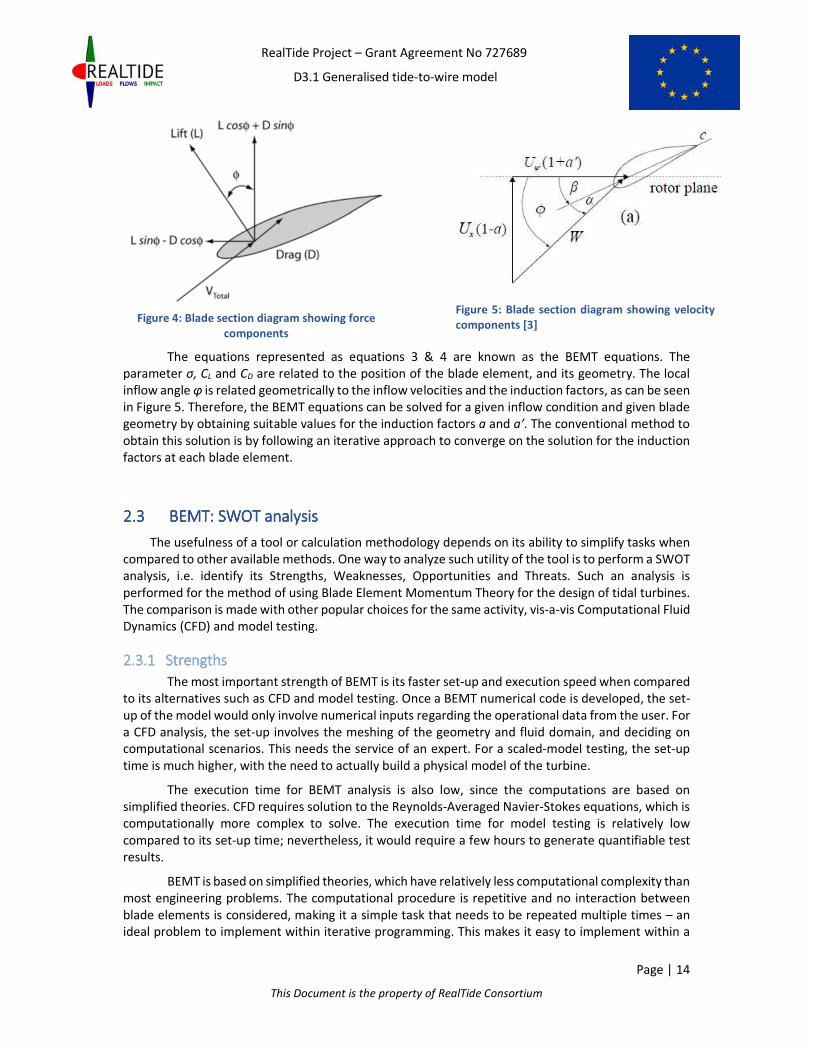
(Eqn. 1 & 2) can be equated in terms of the lift (L) and drag (D) of the airfoil section (See Figure 4).
Solving these equations algebraically, we get the induction factors in terms of the lift and drag
coefficients (CL and CD), as shown in equations 3 & 4. $��$ � %�&' ()* +,&- *./ +�0 *./� + ...... (Eqn. 3)
$�,$ � %�&' *./ +�&- ()* +�0 *./ + ()* + ...... (Eqn. 4)
where σ is defined as the local solidity ratio (1 � 23�45, B = no: of blades, c = chord length, r = radial
location of blade element)
RealTide Project – Grant Agreement No 727689
D3.1 Generalised tide-to-wire model
Page | 14
This Document is the property of RealTide Consortium
Figure 4: Blade section diagram showing force
components
Figure 5: Blade section diagram showing velocity
components [3]
The equations represented as equations 3 & 4 are known as the BEMT equations. The
parameter σ, CL and CD are related to the position of the blade element, and its geometry. The local
inflow angle φ is related geometrically to the inflow velocities and the induction factors, as can be seen
in Figure 5. Therefore, the BEMT equations can be solved for a given inflow condition and given blade
geometry by obtaining suitable values for the induction factors a and a’. The conventional method to
obtain this solution is by following an iterative approach to converge on the solution for the induction
factors at each blade element.
2.32.32.32.3 BEMTBEMTBEMTBEMT: SWOT analysis: SWOT analysis: SWOT analysis: SWOT analysis
The usefulness of a tool or calculation methodology depends on its ability to simplify tasks when
compared to other available methods. One way to analyze such utility of the tool is to perform a SWOT
analysis, i.e. identify its Strengths, Weaknesses, Opportunities and Threats. Such an analysis is
performed for the method of using Blade Element Momentum Theory for the design of tidal turbines.
The comparison is made with other popular choices for the same activity, vis-a-vis Computational Fluid
Dynamics (CFD) and model testing.
2.3.12.3.12.3.12.3.1 StrengthsStrengthsStrengthsStrengths
The most important strength of BEMT is its faster set-up and execution speed when compared
to its alternatives such as CFD and model testing. Once a BEMT numerical code is developed, the set-
up of the model would only involve numerical inputs regarding the operational data from the user. For
a CFD analysis, the set-up involves the meshing of the geometry and fluid domain, and deciding on
computational scenarios. This needs the service of an expert. For a scaled-model testing, the set-up
time is much higher, with the need to actually build a physical model of the turbine.
The execution time for BEMT analysis is also low, since the computations are based on
simplified theories. CFD requires solution to the Reynolds-Averaged Navier-Stokes equations, which is
computationally more complex to solve. The execution time for model testing is relatively low
compared to its set-up time; nevertheless, it would require a few hours to generate quantifiable test
results.
BEMT is based on simplified theories, which have relatively less computational complexity than
most engineering problems. The computational procedure is repetitive and no interaction between
blade elements is considered, making it a simple task that needs to be repeated multiple times – an
ideal problem to implement within iterative programming. This makes it easy to implement within a
RealTide Project – Grant Agreement No 727689
D3.1 Generalised tide-to-wire model
Page | 15
This Document is the property of RealTide Consortium
computer code, without having the need for advanced computational techniques such as geometry
discretization or differential equation solutions.
Similar to the other available tools, BEMT also has the advantage of being reusable. Once
developed, the same tool can be used for different turbine geometries or for different operating
scenarios. This is the same case with a CFD software package or a scaled-model. However, the
advantage of BEMT is the relatively lower set-up time for a new project.
2.3.22.3.22.3.22.3.2 WeaknessesWeaknessesWeaknessesWeaknesses
The basis of BEMT is on simplified theories such as conservation of momentum and
segmentation of a blade to different blade elements. These theories work perfectly only in idealized
conditions and have a lot of theoretical assumptions as well. They do not necessarily reflect a realistic
scenario. BEMT ignores many such realistic intricacies to make the computations simpler and faster.
Along with the assumptions on the physics of the problem, BEMT also makes simplifications of
the inflow conditions. A dynamic variation of the particle velocities are not considered in simple BEMT.
The simple BEMT works based on static lift and drag data of aerofoil sections, and the dynamic effects
such as dynamic stall are not inherently included in it. Such effects are case-dependent and also
depend on the time hysteresis of the flow, and thus are difficult to incorporate in a simplified theory
such as BEMT.
2.3.32.3.32.3.32.3.3 OpportunitiesOpportunitiesOpportunitiesOpportunities
Based on the strengths and weaknesses of BEMT, its best possible use would be in the
preliminary design stage. At this stage, the time required for set-up and execution is a crucial factor;
and BEMT has an edge over the other tools in this factor. It is also inexpensive in terms of cost and
computations, making it an ideal choice. This would be beneficial for the designer to finalize the basic
design and structural parameters, as a BEMT tool would allow him to simulate multiple scenarios in
less time.
Another possible application of BEMT would be to implement it within design optimization
algorithms. Such algorithms work on repeating the same calculation for different input parameters and
then converging to an optimum solution. Considering the fact that a large number of calculations with
varying input parameters needs to be performed, the use of BEMT instead of CFD would be ideal for
this scenario.
To address the major weakness of BEMT, i.e. the theoretical simplifications, empirical models
can be used as corrections to simulate these effects. Analytical and statistical models, which predict
such behaviour are available in existing literature, and in many cases have been validated with
experimental results as well. Implementing such empirical models on top of BEMT would give an ideal
opportunity to improve the accuracy and reliability of this method.
2.3.42.3.42.3.42.3.4 Threats Threats Threats Threats
The most serious threat for BEMT is to determine how accurate it simulates a real-world
scenario. Since it does not capture the entire physics of the problem, its accuracy depends on the
validity of the assumptions and the empirical models. For these reasons, the accuracy of the tool needs
to be validated with available test results or with experimental data.
Being relatively faster than CFD and model testing is the major advantage of BEMT. When
implementing additional empirical models, it should be taken note that the computational speed of
the BEMT tool is not severely compromised. Efficient and simple correction modules are to be
implemented so that its ‘Unique Selling Proposition’ (USP) of fast execution remains intact.

RealTide Project – Grant Agreement No 727689
D3.1 Generalised tide-to-wire model
Page | 16
This Document is the property of RealTide Consortium
As mentioned earlier, BEMT simplifies a complex problem into a simple problem that needs to
be solved a multiple number of times. While this allows the problem to be implemented within
iterative loops, the number of computations can play a significant role here. The code should be able
to decide on this quantity keeping a balance between computational speed and accuracy of results.
The use of semi-empirical models to simulate dynamic events is complicated. Dynamic events
such as turbulent inflow, dynamic stall, and vortex formation are difficult to explain and quantify. This
would mean that the numerical models that simulate such events would definitely involve complex
mathematical equations and solutions. This subdues the strength of BEMT in the matter of
computational complexity.
2.3.52.3.52.3.52.3.5 SummarySummarySummarySummary
The SWOT analysis provides valuable insight into the applicability of BEMT into real-world
design problems. A summary of these points is represented in Figure 6. Although these points are non-
exhaustive, they give an overall idea about where and how BEMT can be applied in design of tidal
turbines.
Figure 6: SWOT analysis of BEMT

RealTide Project – Grant Agreement No 727689
D3.1 Generalised tide-to-wire model
Page | 17
This Document is the property of RealTide Consortium
3333 IMPIMPIMPIMPROVEMENTS TO BEMTROVEMENTS TO BEMTROVEMENTS TO BEMTROVEMENTS TO BEMT
Although the Blade Element Momentum theory provides a fundamental framework for analyzing
the performance of a tidal turbine, it is very simplistic in its formulation. There are different factors of
the fluid inflow and dynamic effects due to the rotation of the rotor that are not considered within this
theory. For this reason, the results from an analytical estimation using BEMT would give considerably
large discrepancies when trying to simulate real-world flow conditions. The main aim of WP3 of
RealTide project is to identify the improvements that could enhance the original BEMT. Also, analytical
methods to implement these improvements onto the BEMT equations are explored in the form of loss
factors, semi-empirical methods and alternate algorithms.
From the review of existing literature, the improvements that could be implemented in BEMT are
as listed below:
a) Losses at blade tip and root
b) High induction factor
c) Wake models
d) Dynamic Stall
e) Single variable optimization
f) Turbulence
g) Loads on tidal turbine
h) Optimization algorithms
In his project report on “Development of a precise BEMT numerical model” [4], Samuel
Hermant has listed many of these corrections and possible methodologies on their implementation.
Further, the user manual for AeroDyn [5] (a series of routines that are widely used for aerodynamic
simulations), explains the various improvements to the BEMT that needs to be considered, as well as
the analytical models used to implement them. These two sources are taken as the major reference
points in identification of the possible improvements and corrections. Further work is done to analyze
each of these improvements from cross-referenced documents and related journals.
3.13.13.13.1 Losses at blade tip and rootLosses at blade tip and rootLosses at blade tip and rootLosses at blade tip and root
The blade element momentum theory does not consider the effects of vortex shedding from the
tip of the blades and its root. Tip vortex shedding is a typical characteristic of fast-moving field rotors
such as ship propellers and turbine blades. Since only the transfer of momentum from the flow field
to the blade rotation is considered within the limits of the theory, the losses due to tip vortex shedding
is not included in the theory. However, these losses are significant and need to be accounted for.
Most of the improved BEMT numerical models account for the tip losses by means of Prandtl
correction factor. This is the same that is implemented in AeroDyn, wherein it is explained that “the
Prandtl model simplifies the wake of a turbine by modeling the helical vortex wake pattern as vortex
sheets that are convected by the mean flow and have no direct effect on the wake itself” [5]. The
theory is characterized by introducing an additional correction factor for the induced velocity field, F
which is given as: 6 � �4 789��:�; where < � 2� =�55 >?@+...... �Eqn. 5�

RealTide Project – Grant Agreement No 727689
D3.1 Generalised tide-to-wire model
Page | 18
This Document is the property of RealTide Consortium
B = Number of blades
R = Blade radius
r = Radial location of the blade element B = Inflow angle
The same correction factor has been reported in Grant Ingram’s work [2] as well, but in a different
form. Samuel Hermant’s research [4] also suggests including the Prandtl correction factor in the design
of turbine blades in order to account for the circulation at blade tips and root due to the pressure
difference between both sides. The losses at hub are also taken into account using a similar correction
factor, but with R being the hub radius instead of the blade radius.
3.23.23.23.2 High Induction FactorHigh Induction FactorHigh Induction FactorHigh Induction Factor
The induction factor is defined as a ratio of change in velocity of flow between the free stream
velocity and the velocity at the blade. The theoretical limit of the axial induction factor, a in BEMT is in
the range of 0 to 0.5. Since �� � ���1 � �� and �0 � ���1 � 2��, at induction factors above 0.5, the
BEMT would predict a negative wake velocity at the turbine blades. This represents the theoretical
limit of the BEMT, whereas in reality this would mean that the wake has become turbulent.
Various methods have been suggested in the literature to account for this effect of the turbulent
wake state and these are discussed subsequently. In the 3rd International Conference on Ocean Energy,
2010 in Bilbao, I. Masters et al had presented a research paper on the implementation of corrections
for high axial induction flow [6]. The various methods that have been suggested are the Glauert
corrections, Spera method and Buhl correction. Another possible correction method that was found
during the literature review was the DNV GL empirical correction formula [7].
The Glauert correction formula was first proposed by Glauert in his book “Airplane Propellers”
[8]. This is an empirical correction to the axial thrust coefficient based on experimental results of
helicopter rotors subjected to flow with large induction factors. Later on, methods such as Spera
method and Buhl correction factor were introduced as alternatives and improvements to this method.
The detailed methodology of the Spera correction is discussed in the work by Shen et al [9].
The Glauert correction was developed considering the entire helicopter rotor, but was then
applied to individual blade elements. In his technical report for National Renewable Energy Laboratory,
Buhl [10] suggested that near the tip of the blade, the tip loss correction would affect the axial
induction factor. Thus, he suggested an improvement to the Glauert’s empirical formulation for the
high induction factor. The validity of Buhl’s correction factor has been restated by I.Masters et al [6]
and also by the AeroDyn Theory Manual [5] which has implemented the Buhl correction factor in their
routines. The correction factors considered in the Glauert method and Buhl’s method are written
below. It is to be noted that the correction is to be applied to the thrust coefficient (CT) based on the
value of the induction factor, a. � � �C D0.143 G H0.0203 � 0.6427�0.889 � MN�O ---- Glauert Correction
MN � PQ G R46 � 0SQ T � G RUSQ � 46T �� ---- Buhl’s Correction Factor
In the “Tidal Bladed Theory Manual” developed by DNV GL [7], a simpler approximation for the
thrust coefficient in case of high induction flows has been proposed. In this method, the thrust
coefficient is represented as a quadratic function of the induction factor, a. The thrust coefficient in
these high induction flows is represented as: MN � 0.6 G 0.61� G 0.79�� ---- Quadratic Correction (DNV GL)
RealTide Project – Grant Agreement No 727689
D3.1 Generalised tide-to-wire model
Page | 19
This Document is the property of RealTide Consortium
There are other empirical relations to characterize the case of high induction factor, as has
been described in the Wind Energy Handbook by Burton et al [11]. Buhl’s correction factor is the one
that is predominantly used in accurate BEMT models. Within the python code, the Buhl’s correction
and the quadratic correction both will be implemented, in order to study the effects these corrections
have on simulating the realistic performance of the tidal turbine.
3.33.33.33.3 Root finding algorithmsRoot finding algorithmsRoot finding algorithmsRoot finding algorithms
The iterative approach followed to find the solution to the induction factors may be
computationally intensive when it comes to depthwise and time-varying input velocity fields that
simulate realistic flow conditions. Moreover, these computations need to be done for each blade
element, at each instant of time. Andrew Ning [12] suggests an alternative approach for optimization
by parameterization of the BEM equations by one variable, i.e. the local inflow angle. This avoids the
need for a two-variable optimization, and one-variable root finding algorithms can be used to
determine an optimum solution. This method has been implemented in the Matlab code developed
by University of Edinburgh, which is referred in the report by Scarlett et al [1].
The advantage of having single-variable equations is that faster optimization algorithms can be
employed. One such optimization algorithm mentioned in the work by Ning [12] is the Brent’s root-
finding algorithm. The possibility of employing such an algorithm to speed up the computation process
needs to be explored during the development of the python code. The solution provided in Ning’s work
includes tip & hub losses as per Prandtl’s method and high inductance correction as per Buhl. The
implementation of alternate correction models and the inclusion of wake models would require a
totally different derivation of the parameterized equations.
3.43.43.43.4 Wake modelsWake modelsWake modelsWake models
The steady inflow assumption of the BEMT is not a realistic assumption for industrial flows. In
reality, the inflow is time variant and the dynamic wake of the inflow needs to be incorporated in the
BEMT model. BEMT is developed based on the assumption that the wake reacts instantaneously to the
changes in blade loading. This means that the solution for a and a’ using the BEMT equations needs to
be obtained for each time step of the dynamic simulation. This is referred to as an equilibrium wake
model, and is computationally intensive. [7]
In reality, the equilibrium wake model does not take into account the time lag for the dynamic
effects to take place. The changes in blade loading change the vorticity that is trailed into the rotor
wake and these effects take a finite time to change the induced flow field. Consideration of this time
lag effect is called as a dynamic wake approach.
An experimental study of this effect has been done in the paper by Whelan et al [13] for the 8th
European Wave and Tidal Energy Conference. The theory manual for Tidal Bladed software [7] also
speaks about this dynamic inflow effect. All the existing literatures agree that the work by Pitt and
Peters [14] is the basis for the development of dynamic inflow effects. In this work, they have used an
added mass effect to model the dynamic inflow effect. The rotor is given an additional added mass
equivalent to 2/3rd of the volume of the fluid in a sphere with the same diameter as the rotor.
Effectively, this modifies both the BEMT equations into first order differential equations of a and a’
respectively. In the work by Celine Faudota et al [15], an implementation of an added mass model is
done for wind turbines, by considering the cylinder approximation for each blade element.
AeroDyn software uses a different method to model the dynamic wake. This method is called the
Generalized Dynamic Wake (GDW) model or acceleration potential method [5]. As mentioned in the
AeroDyn manual, the GDW method is based on potential flow and is a solution to the Laplace’s

RealTide Project – Grant Agreement No 727689
D3.1 Generalised tide-to-wire model
Page | 20
This Document is the property of RealTide Consortium
equation in the fluid domain. This provides for a more general pressure distribution across the rotor
plane. The induced velocities are represented as a set of first order differential equations in an
ellipsoidal coordinate system. These can be solved using non-iterative techniques and the method
used in AeroDyn is the fourth-order Adams-Bashford-Moulton method. The journal article by Maniaci
and Li [16] describes how they have implemented the added mass model in AeroDyn for a marine
hydrokinetic turbine.
TU Delft has undertaken an experimental and numerical validation study of the various
engineering models of dynamic inflow [17]. The paper compares 3 models of dynamic inflow, namely
the Pitt-Peters model, the Oye dynamic inflow model and the ECN’s dynamic inflow model. The Oye
dynamic inflow model is also used by Nevaleinen et al for a sensitivity analysis in predicting the non-
uniform loads that a turbine would experience when there is a sudden change in its operating
conditions. [18].
3.53.53.53.5 Dynamic Stall modelDynamic Stall modelDynamic Stall modelDynamic Stall model
The variation of fluid velocity over the rotor disk creates unsteady angles of attack at the blade
sections. These cause dynamic stall events and need to be accounted for by a dynamic stall model. In
AeroDyn [5], the dynamic stall model proposed by Beddoes and Leishman is used. An example of the
implementation of this model is provided by Hansen et al [19]. While considering the unsteady
hydrodynamics of a full-scale tidal turbine, Scarlett et al [1] have also considered the implementation
of a dynamic stall model coupling it with the blade element momentum theory. The dynamic stall
implemented in TidalBladed also follows the Beddoes-Leishman model. The code developed at
University of Edinburgh features the Sheng model, which is based on the 3rd generation dynamic stall
model of Beddoes [3].
An understanding of the dynamic stall phenomena is necessary to ensure accurate
implementation of the same within the code. In their technical report on a comparison between
various dynamic stall modules [20], Reddy and Kaza classifies the various methods used to represent
semi-empirical models of dynamic stall into the following categories:
(i) Corrected angle of attack
(ii) Synthesization of experimental data to compact expressions
(iii) Describe lift and moment coefficients as ordinary differential equations
The Beddoes-Leishman model is a combination of all these 3 category of representation of
semi-empirical formulation and is used as the basis for development of many of the actively used
dynamic stall modules today. Therefore, this model will be used for understanding and explaining the
dynamic stall phenomenon, in the following paragraphs. A summary of the Beddoes aerodynamic
model is given by J Beedy [21]. The basic Beddoes-Leishman model is explained by Leishman in his
book, “The Principles of Helicopter Aerodynamics” [22]. A modified Beddoes-Leishman model, as
implemented in the University of Edinburgh BEMT code, has been proposed by Sheng et al [23]. These
documents have been used as the chief references for explaining the dynamic stall phenomenon.
Dynamic stall refers to the stalling of an aerofoil, or lifting surface, during unsteady flow
condition. During such conditions, there is a significant delay in the stall of the airfoil when compared
to the static case, and this may allow the airfoil to attain a much larger value of lift. The conventional
stages of dynamic stall are represented in Figure 7.

RealTide Project – Grant Agreement No 727689
D3.1 Generalised tide-to-wire model
Page | 21
This Document is the property of RealTide Consortium
Figure 7: Conventional stages of Dynamic Stall [22] [24]
A correct representation of dynamic stall should consider the effects of all these changes in a
dynamic working environment. Of principal importance is the increased lift generated by the
convecting vortex, which can generate unexpectedly high forces and rotational speeds for the tidal
turbine. The dynamic stall model should account for time constants that trigger the onset of flow
separation at the leading-edge, complete convection of the vortex up to the trailing-edge and the
reattachment of the flow at lower angle of attacks.
3.63.63.63.6 SingleSingleSingleSingle----variable optimizationvariable optimizationvariable optimizationvariable optimization
The iterative approach followed to find the solution to the induction factors may be
computationally intensive when it comes to depthwise and time-varying input velocity fields that
simulate realistic flow conditions. Moreover, these computations need to be done for each blade
element, at each instant of time. Andrew Ning [12] suggests an alternative approach for optimization
by parameterization of the BEM equations by one variable, i.e. the local inflow angle. This avoids the
need for a two-variable optimization, and one-variable root finding algorithms can be used to
determine an optimum solution. This method has been implemented in the Matlab code developed
by University of Edinburgh, which is referred in the report by Scarlett et al [1].
The advantage of having single-variable equations is that faster optimization algorithms can be
employed. One such optimization algorithm mentioned in the work by Ning [12] is the Brent’s root-
finding algorithm. The possibility of employing such an algorithm to speed up the computation process
needs to be explored during the development of the python code. The solution provided in Ning’s work
includes tip & hub losses as per Prandtl’s method and high inductance correction as per Buhl. The
implementation of alternate correction models and the inclusion of wake models would require a
totally different derivation of the parameterized equations.
3.73.73.73.7 Turbulence ModelTurbulence ModelTurbulence ModelTurbulence Model
Another possible improvement in the BEMT model that can be implemented is to introduce a
robust turbulence model that can account for the turbulent nature of the flow. One of the possibilities

RealTide Project – Grant Agreement No 727689
D3.1 Generalised tide-to-wire model
Page | 22
This Document is the property of RealTide Consortium
of such implementation is the TurbSim program developed by the National Renewable Energy
Laboratory, Colorado [25]. TurbSim is efficient in terms of CPU (Central Processing Unit) and memory
usage, and developed specifically considering the needs of the wind turbine environment. An
extension of this could be done to implement in a tidal turbine environment. A user guide for the use
of the TurbSim program is available [26] and the same can be used to include a turbulence model
within the Python program.
Other examples of turbulence models that have been implemented for analysis of tidal turbines
are found in Tidal Bladed [7]. The software uses a three-dimensional turbulence model, with separate
time history for every point within a rectangular grid on the rotor plane. The turbulence models
adopted are the von Karman model, improved von Karman model, Kaimal model and the Mann model.
3.83.83.83.8 Loads on TidaLoads on TidaLoads on TidaLoads on Tidal Turbinesl Turbinesl Turbinesl Turbines
One of the major uncertainties in any structural engineering problem is the uncertainty in
determining the loads that act on the structure. In the case of a tidal turbine also, this is a major
uncertainty. Even though the tidal flow can be predicted, the presence of free surface waves, ocean
currents and the turbulence characteristics of the flow make the prediction of the incoming flow to
the tidal turbine a matter of uncertainty.
The evaluation of wave induced velocities has its own further uncertainties since these are
random and stochastic in nature. In deep sea, a regular wave field can be assumed thereby applying
linear wave theory to determine the wave loads to a decent accuracy. The same has been proposed in
the work by Celine Faudot et al [15]. Such an estimation of the loads is essential in the structural design
of the blades, which is one of the expected outcomes from the research and internship.
Apart from the use of regular wave theory, empirical expressions that are developed from
industrial experience can also be used for this purpose. One such example is the classification
guidelines by Bureau Veritas for Current and Tidal Turbines [27]. These guidelines are typically used
for the structural design of the blade, hub, nacelle and duct. Such guidelines and iterative processes
are very important while creating a design optimization loop within the program algorithm.
The work by Chul et al [28] from Inha University, Incheon, Korea highlights the use of the
deformed blade shape for accurate estimation of the power generated by a tidal turbine. Essentially
this is a case of fluid-structure interaction wherein the fluid domain solution is obtained by
Computational Fluid Dynamics (CFD) and then the deformation of the blade calculated using finite
elements. This deformed shape is then used to modify the flow field and the power output is predicted.
3.93.93.93.9 Optimization AlgorithmsOptimization AlgorithmsOptimization AlgorithmsOptimization Algorithms
One of the main expected outcomes from the internship is to develop a tool that is robust enough
to aid the designer in the preliminary design stage. When trying to efficiently implement a design tool
at this stage, useful optimization routines that would reduce the iterative work done by the designer
are options that should be considered. Therefore, the literature review was also aimed at finding such
optimization algorithms which could be used while developing the code.
In the paper by I. Masters et al [29], a robust BEMT model using combined Monte Carlo and
sequential quadratic optimization. During the design of the tidal turbine, both the induction factors –
axial induction factor, a and the tangential induction factor, a’ – are unknown. The usual procedure is
to assume one and iteratively solve for the other. This paper describes how a Monte Carlo simulation
can be used to figure out an optimized solution for these both induction factors.
Apart from that, once could also employ the genetic algorithm methods that are available within
the Python libraries. However, in order to develop an efficient methodology for optimization, it is

RealTide Project – Grant Agreement No 727689
D3.1 Generalised tide-to-wire model
Page | 23
This Document is the property of RealTide Consortium
imperative to first define a smooth and streamlined process for computation. Once this is achieved,
and the critical parameters identified, then only can a suitable optimization algorithm be employed.
Therefore, the focus at the preliminary stage is to develop a code that focuses on predicting the force
outputs and electrical parameters from the tidal turbine operating conditions. The implementation of
an optimization algorithm will be studied further in detail and attempted to implement at a later stage.

RealTide Project – Grant Agreement No 727689
D3.1 Literature Review - Evaluation of force on tidal blades
Page | 24
This Document is the property of RealTide Consortium
4444 EXISTING BEMT TOOLSEXISTING BEMT TOOLSEXISTING BEMT TOOLSEXISTING BEMT TOOLS
While developing a code that is based on Blade Element Momentum theory, it is vital to take a
look at the existing tools that use this framework. The two industries that have been identified as
suitable for implementation of this theory are the Tidal turbines and wind turbines. Accordingly, a
study on the existing software tools that have implemented the BEMT has been conducted
A brief overview of the manner in which the BEMT has been implemented and the extent to which
the BEMT improvements have been included in these software packages is analysed within the scope
of this section. A comprehensive summary of these improvements is provided in a tabular format at
the end of the section. The software packages thus identified are as follows:
4.14.14.14.1 Software PackagesSoftware PackagesSoftware PackagesSoftware Packages
a) Tidal Bladed:
Tidal Bladed is an integrated software package used in the design, performance and loading
calculations of tidal turbines. [7] The software was developed by Garrad Hassan Ltd., which was
later acquired by DNV GL. The software is a comprehensive tool, which implements BEMT with
many of its improvements. The effects of dynamic stall can also be analysed in an unsteady flow.
It can take into account various environmental effects such as waves and ocean currents. Also,
the influence of towers, turbulence model and cavitation inception criteria are also included
features of the software.
b) University of Edinburgh (UEDIN) Code:
The UEDIN code is a series of Matlab based routines that can be used to predict the force
output from a tidal turbine. The code has incorporated a dynamic stall model, which can give
accurate results for unsteady flow cases. The code is suited primarily to take an input from the
sea test results for tidal turbines, projects such as ReDAPT [30]. Flow characteristics such as effects
of waves, currents, and turbulence are inherently included within the input velocity profile.
c) HydrOcean Code:
Similar to the Matlab code of UEDIN, a sequence of Matlab routines were developed at
HydrOcean, Nantes, France to aid in the analysis of tidal turbines. Although not as robust as the
UEDIN code for unsteady flows, the code is inclusive of many of the BEMT improvements such as
tip loss, high induction factor and dynamic wake effects. The work done in the development of
the code could be used as a basis for study on the various improvements of BEMT and their
implementations within a coded language [4]. The code has also implemented a Matlab based
genetic algorithm to aid in an optimization process.
d) HARP_Opt:
The HARP_Opt (Horizontal Axis Rotor Performance Optimization) code utilizes a multiple
objective genetic algorithm and blade-element momentum (BEM) theory flow model to design
horizontal-axis wind and hydrokinetic turbine rotors [31]. The code is a development by the
National Renewable Energy Laboratory (NREL), Colorado aimed at the design procedures of tidal
turbines. It uses the WT_Perf BEM theory code, which is also the basis for their aerodynamic tools
such as FAST and AeroDyn. However, the tool focuses on design optimization and hence focuses
mainly on a static analysis, without considering the effects of dynamic stall.

RealTide Project – Grant Agreement No 727689
D3.1 Generalised tide-to-wire model
Page | 25
This Document is the property of RealTide Consortium
e) FAST/AeroDyn:
AeroDyn is a set of routines primarily meant for analysis of aerodynamic performance of
wind turbines [5]. It is also developed at the National Renewable Energy Laboratory, Colorado.
Even though designed specifically for wind turbines, the routines present in the software package
have relevant applications to the domain of tidal turbine design as well. Various improvements
that have been discussed in Section 3 have been incorporated within AeroDyn. The dynamic wake
effect is included in the form of an acceleration potential method, which is a potential flow
solution to the Laplace equation within the fluid domain. The dynamic stall module present in
AeroDyn is also well developed and uses the Beddoes and Leishman model.
f) AERFORCE:
AERFORCE is a Fortran-based package of subroutines for calculation of aerodynamic force
of wind turbine rotors, developed by the FFA, The Aeronautical Research Institute of Sweden [32].
The routine is adapted to work on time simulations. The output from the code is wind and blade
velocities and blade forces at a sequence of time steps. This is designed such that the output can
be taken into an aero-elastic code further simulations of blade response to aerodynamic loads.
The FFA has also developed a dynamic stall model in FORTRAN to work along with
AERFORCE. This is a 2D unsteady airfoil dynamics which is an implementation of the Beddoes-
Leishman dynamic stall model [33]. The literature gives a step-wise procedure of the
implementation of the Beddoes-Leishman model, the framework of which is similar to that which
could be used in the dynamic stall module for tidal turbines.
4.24.24.24.2 Input Input Input Input
The first criteria that is chosen for comparison is the manner in which these software packages
accept input data from the user. Based on the type and purpose of the software, this format might
vary.
4.2.14.2.14.2.14.2.1 Velocity ProfileVelocity ProfileVelocity ProfileVelocity Profile
Since we are dealing with a flow environment here, the primary input data required is the
manner in which the inflow velocity is provided to the code. In the real case scenario, if an Eulerian
frame of reference approach is used, the particles on a spatial grid just aft of the turbine would have
velocity components in the three-directions. Moreover, the turbulence characteristics of the flow is
not represented by these velocity components, and that would probably require a separate treatment.
The turbulence characteristics (such as turbulence intensity) may also need to be considered to give a
more accurate representation of the inflow conditions.
It is not practical to represent all the physical characteristics of the inflow within the framework
of developing a computationally inexpensive numerical code. Therefore, the flow characteristics need
to be suitable simplified, but still sufficient to have a good representation of the real physical flow.
When considering the velocity profile, the following attributions to variations in the velocity profile
may be identified:
(i) Variation along z – depthwise varying velocity profile
(ii) Variation along y – changing velocity profile in the transverse direction
(iii) Variation with time – dynamic inflow condition
(iv) Turbulence characteristics of the inflow
(v) Effects of rotor rotation on the inflow

RealTide Project – Grant Agreement No 727689
D3.1 Generalised tide-to-wire model
Page | 26
This Document is the property of RealTide Consortium
Table 1 shows a descriptive comparison of the various software packages mentioned in Section
4.1 with respect to their input parameters. The five attributes mentioned above are analysed
specifically. Table 2 shows a summary of these capabilities in each of these software package. It is to
be noted that the comparison is based mainly on the literature available of these software packages.
Only limited or minimal user experience is involved; hence the comparison may only be taken as a
superficial approach and may not encompass the entire functionality of the software.
Table 1: Input velocity profile for various software packages
Software Description
Tidal Bladed In Tidal Bladed, the input velocity conditions are derived from the environmental
conditions. The user inputs the current, wave, wind and tidal conditions. The
velocity profile, with variations along depth and time, are computed based on this.
Also, the software implements 3-dimensional turbulence models such as von
Karman model, Kaimal model and Mann model. There is no explicit mention about
taking into account the effects of the rotation of the turbine affecting the flow
field.
UEDIN Code The UEDIN code was designed to analyze results from the ReDAPT project
measurements. The input data for this code is the velocity profile measured by the
sensors in the real-sea conditions. As a result, this inherently includes the
variations within spatial and time co-ordinates. However, the spatial grid is
simplified to only account for variations along the depth; the transverse variations
are not taken into account. However, the velocity of the blades is adjusted for the
azimuthal position of the blade. The turbulence characteristics are measured
within the ReDAPT project; but these values are not incorporated within the input
velocity profile.
HydrOcean
Code
The HydrOcean code is designed for performing analysis of tidal turbines in a
constant stream velocities. However, the code can take into account the time
variation of the stream velocities, so that the same may be analyzed for the
dynamic wake effect.
HARP_Opt As an optimization software, HARP_Opt prioritizes on operating conditions of the
turbine. Thus, the stream velocity is taken as constant along the entire diameter
of the blade, i.e. no variation of velocity within a spatial grid is considered.
However, variation in rotor speed and pitch of the blades are considered as an
input condition. The variation in rotor speed induces a dynamic effect into the
inflow, and hence a variation with time is effectively.
FAST/AeroDyn AeroDyn is one of the most advanced tools available for the analysis of wind
turbines. The input can be manipulated to provide the velocity profile within a
rectangular spatial grid. The turbulence of the flow can also be include by applying
the TurbSim turbulence modeled by NREL.
AERFORCE AERFORCE is also designed for a constant stream velocity condition; but the
dynamic effects are considered with a time variation in velocity modeled by a
quasi-steady value of the induction factor. The effects of turbulence and rotor
rotation are not considered in the code.

RealTide Project – Grant Agreement No 727689
D3.1 Generalised tide-to-wire model
Page | 27
This Document is the property of RealTide Consortium
Table 2: Capabilities of software package w.r.t. input velocity profile
Software Along depth Transversely With time Turbulence Rotor Speed
Tidal Bladed Yes Yes Yes Yes ---
UEDIN Code Yes --- Yes --- ---
HydrOcean Code --- --- Yes --- ---
HARP_Opt --- --- Yes --- Yes
FAST/AeroDyn Yes Yes Yes Yes ---
AERFORCE --- --- Yes --- ---
4.2.24.2.24.2.24.2.2 Lift and Drag CoefficientsLift and Drag CoefficientsLift and Drag CoefficientsLift and Drag Coefficients
The performance of the tidal turbine depends on its geometrical parameters such as the blade
shape, and thickness. The type of blade section (aerofoil profile) at each blade element would
determine its lift and drag coefficients and subsequently the force generated at the blade element.
This is a design parameter and needs to be provided by the user.
For greater accuracy of computations, larger number of blade elements may be considered.
However, the aerofoil profile at each of these sections might be different and hence would have
different lift and drag characteristics. These characteristics are not so straightforward to calculate from
the geometry of the section, and typically would require a tabular input from the user. All in all, this
would require a massive databank input from the user; and hence, the manner in which this is handled
is also of extreme importance while designing the architecture of the code.
Another factor to consider is the range of angle of attacks for which the lift and drag coefficients
are provided. Typically, the aerofoil lift and drag data are only provided for a range of angle of attacks,
say -30o to +30o, as the angle of attack in the static regime usually stays within this range. However,
when considering the performance in cases of dynamic events, the angle of attack can be well in excess
of the steady state stall angle. Moreover, when an iterative solution is considered, the range of angle
of attack should be large enough to allow convergence of the solution.
The attributes that are important while considering the lift and drag input data may be
summarized under the following headings:
(i) Range of angle of attacks
(ii) Extrapolation of lift and drag data
(iii) Multiple aerofoil profiles

RealTide Project – Grant Agreement No 727689
D3.1 Generalised tide-to-wire model
Page | 28
This Document is the property of RealTide Consortium
Table 3: Comparison of lift-drag coefficient input data
Software Description
Tidal Bladed Tidal Bladed is provided with features such that multiple aerofoil profiles can be
defined at different blade element. The lift and drag coefficients of each of these
sections must be input by the user. However, the user can save already input blade
data to be included for a later calculation. The software also has a feature to
extrapolate the input data to an angle of attack range of -180o to +180o using the
Viterna Extrapolation method.
UEDIN Code The UEDIN code takes the blade profile data directly as provided for the ReDAPT
project. Since this blade data does not contain the lift and drag data for the entire
data range (-180o to +180o angle of attack range), the software uses the Viterna
extrapolation method to achieve this. The blade used in the ReDAPT project does
not have multiple aerofoil profiles; hence the UEDIN code does not have to
consider this complexity.
HydrOcean
Code
In this code, different aerofoil profiles are considered for each element. But the
user needs to provide the lift and drag data for each of them. Unlike the other
codes, the lift-drag coefficients are not provided as functions of Reynolds number,
but instead for the particular thickness-chord ratio of the particular blade element.
This avoids the problem of having a huge CL, CD database; but the issue is that the
variation with Reynolds number is not considered (since the code only considers a
fixed stream velocity).
HARP_Opt HARP_Opt has features to optimize the geometry of the blades. This means that
the user has to provide the lift and drag coefficient at each blade element for each
angle of attack. However, the software has inbuilt optimization algorithms that
can provide an optimum thickness-chord ratio at each blade element.
FAST/AeroDyn AeroDyn also explains the Viterna extrapolation as a method to fill in the data for
the angle of attack range between -180o and +180o. But this is not a capability of
AeroDyn, but it can be done using another NREL program named FoilCheck. The
user needs to provide the extrapolated data for the entire range of angle of
attacks; but can obtain assistance from FoilCheck for each blade section.
AERFORCE The AERFORCE manual specifies that the lift and drag data needs to be provided
by the user for the entire range of expected angle of attacks. There is no presence
of any extrapolation algorithms within the software. Since nothing is explicitly
mentioned about considering multiple blade sections, it is assumed that the same
is incorporated within the code.
4.2.34.2.34.2.34.2.3 Environmental ConditionsEnvironmental ConditionsEnvironmental ConditionsEnvironmental Conditions
The environmental conditions that are relevant to the inflow of a tidal turbine are the tides,
waves and ocean currents. It might be of interest to the designer to obtain the performance of the
turbine for a particular environment condition. More importantly, these environmental conditions
would have a bearing on the time dependant velocity component at the inflow of the turbine. Table 4
shows the way in which these environmental conditions are considered within each of these software.
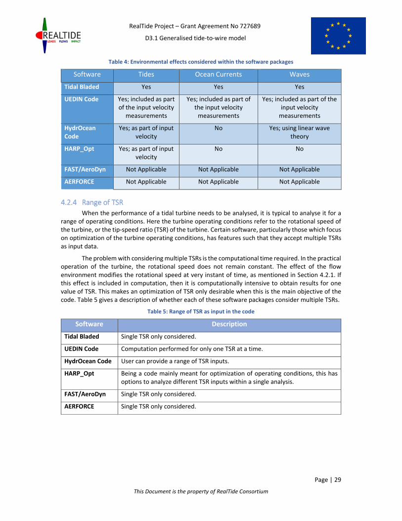
RealTide Project – Grant Agreement No 727689
D3.1 Generalised tide-to-wire model
Page | 29
This Document is the property of RealTide Consortium
Table 4: Environmental effects considered within the software packages
Software Tides Ocean Currents Waves
Tidal Bladed Yes Yes Yes
UEDIN Code Yes; included as part
of the input velocity
measurements
Yes; included as part of
the input velocity
measurements
Yes; included as part of the
input velocity
measurements
HydrOcean
Code
Yes; as part of input
velocity
No Yes; using linear wave
theory
HARP_Opt Yes; as part of input
velocity
No No
FAST/AeroDyn Not Applicable Not Applicable Not Applicable
AERFORCE Not Applicable Not Applicable Not Applicable
4.2.44.2.44.2.44.2.4 Range of TSRRange of TSRRange of TSRRange of TSR
When the performance of a tidal turbine needs to be analysed, it is typical to analyse it for a
range of operating conditions. Here the turbine operating conditions refer to the rotational speed of
the turbine, or the tip-speed ratio (TSR) of the turbine. Certain software, particularly those which focus
on optimization of the turbine operating conditions, has features such that they accept multiple TSRs
as input data.
The problem with considering multiple TSRs is the computational time required. In the practical
operation of the turbine, the rotational speed does not remain constant. The effect of the flow
environment modifies the rotational speed at very instant of time, as mentioned in Section 4.2.1. If
this effect is included in computation, then it is computationally intensive to obtain results for one
value of TSR. This makes an optimization of TSR only desirable when this is the main objective of the
code. Table 5 gives a description of whether each of these software packages consider multiple TSRs.
Table 5: Range of TSR as input in the code
Software Description
Tidal Bladed Single TSR only considered.
UEDIN Code Computation performed for only one TSR at a time.
HydrOcean Code User can provide a range of TSR inputs.
HARP_Opt Being a code mainly meant for optimization of operating conditions, this has
options to analyze different TSR inputs within a single analysis.
FAST/AeroDyn Single TSR only considered.
AERFORCE Single TSR only considered.

RealTide Project – Grant Agreement No 727689
D3.1 Generalised tide-to-wire model
Page | 30
This Document is the property of RealTide Consortium
4.34.34.34.3 BEMT ImprovementsBEMT ImprovementsBEMT ImprovementsBEMT Improvements
Blade Element Momentum Theory is not entirely representative of the flow physics that occurs
during the flow of water around the rotating blades of a tidal turbine. The theory, developed in a near-
ideal framework, needs to be supported with various improvements, as discussed in Section 3, in order
to simulate realistic flow environments. Incorporating complex improvements would however
increase the computational complexity of the algorithm, and as such defeat the purpose of developing
the code; which is to function as a fast, viable and reasonably accurate alternative in the preliminary
design stage for viscous flow solvers in the domain of computational fluid dynamics.
To define the extent to which these improvements have to be implemented, the literature
review should also encompass the manner in which they are implemented within existing software
packages. Within this section, an overall summary of the BEMT improvements implemented in each
software is provided. For the sake of simplicity, the list of improvements are split into two tables, Table
6 and Table 7; the former showing a list of basic BEMT improvements and the latter describing about
the improvements related to dynamic flow effects.
Table 6: Comparison of basic BEMT improvements
Software Tip & Hub Losses High Induction Factor Computation algorithm
Tidal Bladed Prandtl theory Quadratic Correction Iterative
UEDIN Code Prandtl theory Buhl correction Ning’s formulation
HydrOcean Code Prandtl theory Quadratic Correction Iterative
HARP_Opt Prandtl theory Buhl correction Iterative
FAST/AeroDyn Prandtl theory Buhl correction Iterative
AERFORCE Prandtl theory Empirical linear curve of
Anderson
Dynamic values of induction
by Snel & Schepers solution
Table 7: Comparison of improvements based on dynamic effects
Software Wake Model Dynamic Stall
Tidal Bladed Dynamic wake model using Pitt and Peters
added mass approximations
Beddoes-Leishman model with a
few modifications
UEDIN Code Equilibrium Wake model Sheng model
HydrOcean Code Dynamic wake model using Pitt and Peters
added mass approximations
None
HARP_Opt Nothing specifically mentioned; but
expected to have the same capability as
AeroDyn
Selig-Du and/or Eggers models
FAST/AeroDyn Generalized Dynamic Wake model or
acceleration potential method
Beddoes-Leishman model
AERFORCE Oye model Beddoes-Leishman model

RealTide Project – Grant Agreement No 727689
D3.1 Generalised tide-to-wire model
Page | 31
This Document is the property of RealTide Consortium
4.44.44.44.4 Other featuresOther featuresOther featuresOther features
Performance analysis of turbines is a generic category that encompasses all these software
packages. Their exact nature of utility might however vary. Some of them are meant to ease the
computations at preliminary design, some are meant as optimization tools, and some are meant as
tools that predict the forces which need to be input into a structural analysis software. Based on these
underlying requirements of each software, they would have certain additional features that cater to
their own domain of expertise. Some of these other features are discussed here, to give a brief insight
of the possibility of their implementations within the RealTide project.
a) Rotational Augmentation:
The rotation of the blades produce an acceleration of the flow towards the trailing edge. This
reduces the adverse pressure gradient to promote flow reattachment and delay separation,
resulting in lift augmentation from the stationary value [34]. This augmentation of lift is considered
within the UEDIN code by making use of the Lindenburg’s model [35] and combined with the
implementation of the dynamic stall model.
b) Optimization:
Many of the tools available are used for a design optimization in the preliminary design stage.
HARP_Opt is one such examples and it employs the Matlab Genetic algorithm to achieve this. The
same is also employed in the HydrOcean code. While the HydrOcean code optimizes the optimum
TSR required for operation, HARP_Opt is a more versatile tool in terms of optimization. HARP_Opt
can perform single or multi-objective optimization, combining objectives of Annual Energy
Production and Maximum Power. It also has a structural optimization algorithm to provide an
optimal shape of the blade.
c) Cavitation prediction:
This feature is employed within Tidal Bladed. It is only a check for the possibility of cavitation,
and does not in any way affect the simulation output. Based on the vapour pressure of water, the
minimum static pressure on each blade element can be computed. This can be then expressed as a
cavitation inception velocity for each blade element. During the computation procedure, once the
magnitude of flow velocity at the blade element is determined, it can then be compared with this
cavitation inception velocity to predict the occurrence of cavitation.
d) Tower influence:
This kind of effects are most predominant in software that are designed for analysis of
wind turbines. AeroDyn includes the modifications of the flow caused by the presence of the wind
turbine tower in their computations. AERFORCE does not have any inherent model to account for
the tower influence, but it specifies that corrections for the tower blockage effects should be
included within the value of the free stream velocity. The software packages that are meant for
tidal turbines usually do not have the effect of this influence. However, Tidal Bladed employs a
detailed model considering the tower shadow effect and wake effects from upstream turbines.
e) Skewed wake correction:
Skewed wake correction is important while considering a non-axisymmetric flow to the
turbine. This is important particularly in the case of turbines that can adjust their angle to the
direction of the inflow. AeroDyn and AERFORCE have employed corrections for such cases of yawed
inflow. AeroDyn uses a method developed by Pitt and Peters; while AERFORCE follows the method
suggested by Stig Oye which in turn uses the Glauert formulation for yawed flows.

RealTide Project – Grant Agreement No 727689
D3.1 Generalised tide-to-wire model
Page | 32
This Document is the property of RealTide Consortium
5555 PROGRAM ARCHITECTUREPROGRAM ARCHITECTUREPROGRAM ARCHITECTUREPROGRAM ARCHITECTURE
Blade Element Momentum Theory predicts the performance for a single blade element rotating
as an annular disc. Extending this theory to a full tidal turbine working in a dynamic environment
involves numerical computations over multiple iterative parameters. Only considering the geometry
of the turbine, this would be in the form of integrating the results for a single blade, and then for
multiple blades. Further, multiple operating conditions present themselves as iterative parameters in
the form of time steps of computations and varying inflow velocities.
These iterative parameters interact with each other over the computational procedure. For
example, the inflow velocity at a blade element which is required for BEMT computations, requires the
knowledge of its instantaneous position. This instantaneous position depends on the rotational speed,
and the blade under consideration. Such interactions between the loop variables would mean that the
program architecture needs to be suitably designed to avoid for any undesirable computational
complexities. Accordingly, it was decided to develop a skeletal framework of the program in the form
of a flowchart, to provide a constructive methodology going forward.
5.15.15.15.1 Iterative loopsIterative loopsIterative loopsIterative loops
The first step in the development of such a framework is to identify the various iterative loops
that would be required in the program. The methodology followed here is to start from the elementary
computation involved and then extent it to obtain a global result of the problem. The elementary
computation involved is the application of the BEMT. The global result is to obtain the prediction of
forces generated by the turbine in a dynamic environment.
The elementary BEMT computations need to be done on every blade element on a blade; hence
it calls for the need of a blade element loop. Then, these computations are to be done for every blade;
and hence a blade loop as well. In constant inflow problems, where there is no variation in velocity
along the radius of the turbine, the result of a single blade could be extended to all other blades.
However, a realistic velocity profile would have different inflow velocities at different locations. This
consideration requires to have an additional iteration over different blades. These are the iterative
loops that need to be included in relation to the geometry of the turbine.
Additionally, the variation in operating conditions also needs to be considered for other iterative
loops. A dynamic environment would mean that the inflow velocity is changing at a discrete time step.
This would require the presence of a Time loop to iterate and compute the calculations at each time
step. Further, it is normal for a designer to assess the performance of the turbine in different rotational
speeds. As a common tidal turbine industrial practice, this rotational speed is not mentioned in terms
of the rotational speed in revolutions per minute; but instead as a non-dimensional rotational speed
known as Tip-Speed Ratio (TSR). This is the ratio between the angular velocity at the tip of the turbine
(= radius of the turbine in m x rotational speed in rad/s) to the inflow velocity at the turbine centre (in
m/s). Hence, this ratio considers the effects of both the factors affecting the operating conditions –
the rotational speed and the inflow current velocity. If the performance of the turbine needs to be
assessed for such multiple TSRs, then a TSR loop also needs to be included.
Within Python, there is also an option for using dataframes instead of looping over variables that
have the same behaviour. A dataframe variable consists of rows of data containing entities with the
same behaviour. The columns of data are the parameters that need to be computed for each of these
rows. In appearance and behaviour, this is similar to an excel worksheet, where the same formula (or
function) can be applied to an entire column. The interesting fact here with regards to a programming
language is that, the columns can have different datatypes, and that makes it versatile for applications.

RealTide Project – Grant Agreement No 727689
D3.1 Generalised tide-to-wire model
Page | 33
This Document is the property of RealTide Consortium
Instead of looping over, say different blade elements, all the blade element geometrical parameters
can be stored inside a dataframe variable, and the computations applied to each row. This is a faster
computational method compared to looping; and also the results are already stored in a logical
sequence, within a single variable, which makes it easier to visualize and analyze.
Considering the utility of the dataframes, in order to reduce the computational time, it would be
beneficial to replace the loop with the maximum number of iterations with a dataframe, and place it
at the interior of the nested loop structure. Typically, this is the time loop for the problem at hand,
since a dynamic problem would require data input at small time steps to have a decent output.
However, the interactions of the time loop with other loop variables needs to be identified. The next
step is to identify such interactions between the loops, so that a logical nested sequence for these
loops could be obtained.
The computational complexity involved in the execution of the Dynamic Stall module is much
more than the actual BEMT computations. This would be evident from the explanation of the former
given in Section 6.3. The replacement of the time loop as a dataframe also speeds up the computations
for the dynamic stall module, as these complex computations can be applied row-wise over multiple
time steps in a single sequence.
Even though this is a feasible idea in a dynamic BEMT analysis wherein only the force outputs are
required, this approach fails when it is necessary to couple the code with an electrical module. In
particular, the problem pertains to the input of the rotational speed for BEMT calculations. If the
variation of rpm throughout the analysis regime is given by the user – it can be constant or varying at
each time step – then this approach can be implemented. However, if the code needs to be coupled
later on with an electrical module, which predicts the rpm at the next time step based on the torque
input at the current time step, then this approach fails. Hence it is not possible to place the time loop
as the inner loop, even though it makes the compuations faster. Consequently, the loop with the next
maximum number of iterations, vis-a-vis the Blade Element loop, is placed as the inner loop.
As all operating conditions are independent of each other, the TSR loop could be placed as the
outer loop. This is also logical, since it is not always that the user wants to analyze performance over
multiple TSRs. Inside the TSR loop, the Time loop is placed, so that it can interact with the electrical
module in future implementations. These are then followed by the Blade loop and finally, the Blade
Element loop, which may be replaced by a dataframe instead of a loop. The program architecture in
its entirety is represented as a flowchart in Figure 8.
The flowchart shows the possible coupling of the electrical module as well. Outside the Blade
loop, one can obtain the total torque produced by the turbine at the current time instant. This can be
fed into the electrical module, which then generates the rotational speed for the next time step. Using
this value of rpm, the computations can be performed for the next time step, and the feedback loop
can be established.
The flowchart also shows the various output characteristics that can be extracted from the program.
The forces produced by the turbine for multiple operating conditions can be extracted out of the
exterior TSR loop, and can be used to determine the optimum operating condition. For each operating
condition, the variation of the forces with time can be extracted outside the time loop. This could be
useful for balancing of the electrical grid, and to predict unsteady loads on the turbine blades. Outside
the blade element loop, one could also extract the elemental forces at each blade element, which can
be then used to compute the shear force and bending moment distributions along the blade, for a
given time step and given operating condition.
The program architecture can also be used to decide on the nature of the variables used in the
program. The BEMT computations would be performed on a dataframe which comprises of all blade
elements on a single blade of the turbine. The result of these computations would be the induction

RealTide Project – Grant Agreement No 727689
D3.1 Generalised tide-to-wire model
Page | 34
This Document is the property of RealTide Consortium
factors a and b, and subsequently the elementary axial and tangential forces, dFax and dFtang
respectively. These are only the force components for a static BEMT. Such dataframe computations
are then done for each blade, and the result integrated to obtain the total thrust and total torque using
static BEMT.
The results from the static analysis are used in the Dynamic Stall module. The dynamic stall
module would use a similar architecture, and the result would be the elementary axial and tangential
forces in dynamic BEMT, dFax_dyn and dFtang_dyn respectively. The process for obtaining thrust and torque
is the same as that for static BEMT. Thus, the output would be the static and dynamic thrust and torque
for each time step. These computations can then be repeated for each TSR.
Now that the framework for computations are defined, it is necessary to define the manner in which
the user input variables – particularly, the blade geometry and the operating conditions - are
incorporated into this framework. This will be discussed in the subsequent sub-headings.
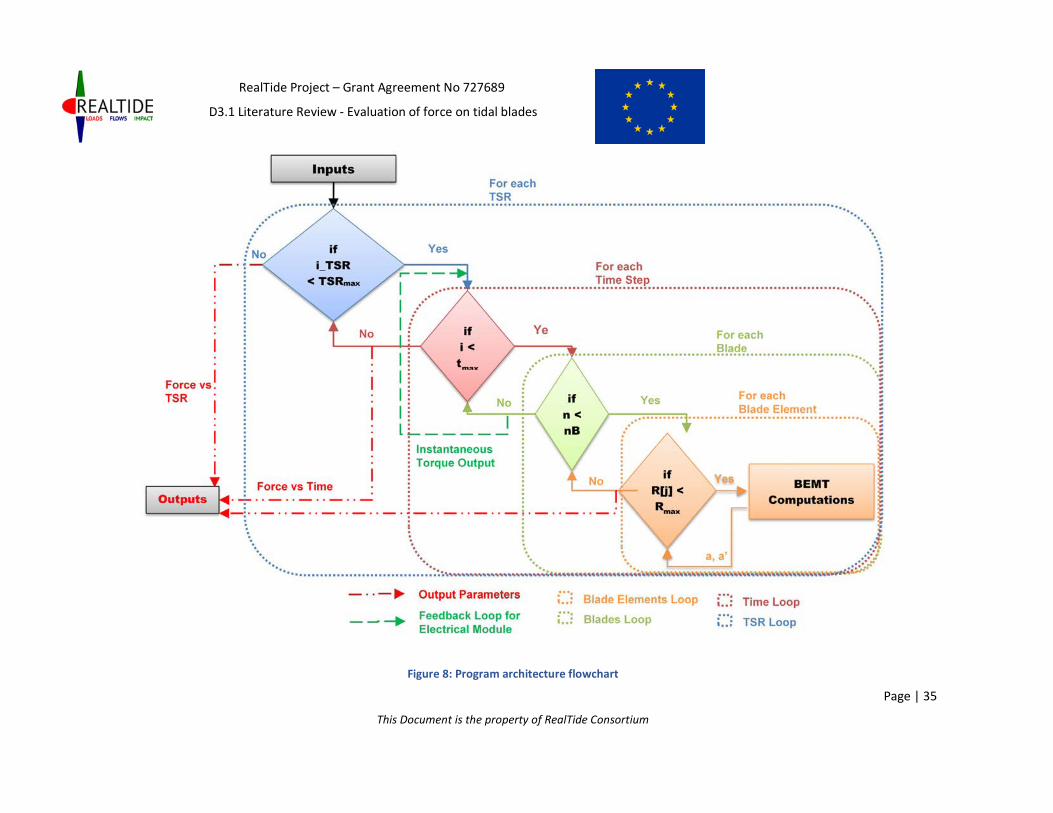
RealTide Project – Grant Agreement No 727689
D3.1 Literature Review - Evaluation of force on tidal blades
Page | 35
This Document is the property of RealTide Consortium
Figure 8: Program architecture flowchart

RealTide Project – Grant Agreement No 727689
D3.1 Literature Review - Evaluation of force on tidal blades
Page | 36
This Document is the property of RealTide Consortium
5.25.25.25.2 Blade Geometry DataBlade Geometry DataBlade Geometry DataBlade Geometry Data
Since the BEMT computations are performed on a dataframe variable that envelops all the blade
elements on a single blade, the corresponding geometrical parameters can be easily included within
this same variable. The geometrical parameters included here are the radial location (r), the chord
length of the blade element (c) and the twist angle at the section (β). A simplified framework is shown
in Table 8.
Table 8: Dataframe structure for different blade elements on a single blade
Blade Element No:
Radial Location (m) Chord (m)
Twist (deg)
0 ..... .... ....
1 ..... .... ....
.... ..... .... ...
Now, the other geometrical parameters that needs to be considered are the lift and drag
coefficients, CL and CD respectively. However, these cannot be directly populated on the dataframe
structure from the user input, since their value depends on the angle of attack at the blade element
and the Reynolds Number of inflow. Both these parameters are dependent on the BEMT solution for
the induction factors. Therefore, the CL and CD values need to be computed during every iterative step
of the BEMT solution. The details of the computational procedure is provided in Section 6. The
dataframe variable only stores the final converged value of CL and CD for each blade element.
5.35.35.35.3 Operating ConditionsOperating ConditionsOperating ConditionsOperating Conditions
5.3.15.3.15.3.15.3.1 Inflow VelocityInflow VelocityInflow VelocityInflow Velocity
As explained in Section 7.2, the inflow velocity data has variation with time and depth, i.e. V = f
(z,t). The user input for this parameter would be the fluctuation of the velocity at a reference point;
and the code computes a depthwise changing profile for each of this time instants. This data needs to
be then assimilated to obtain the axial velocity of inflow for each blade element. This depends on the
instantaneous position of the blade element.
Knowing the initial position of the blade element and its rotation speed, the instantaneous
position of the blade element for a time step tn can be obtained. The velocity at the reference point at
time tn is then obtained from the user input data. Applying the power law (user input, as specified in
Section 7.2), an interpolation function is generated for the velocity as a function of the depth, i.e. V =
f (z). Using the instantaneous position of the blade element as the input to this interpolation function,
the axial velocity of inflow at the blade element can be found.
5.3.25.3.25.3.25.3.2 Rotation SpeedRotation SpeedRotation SpeedRotation Speed
The instantaneous rotation speed of the turbine is another input variable that needs to be
incorporated in the dataframe. Unlike the blade geometry parameters and inflow velocity, this

RealTide Project – Grant Agreement No 727689
D3.1 Generalised tide-to-wire model
Page | 37
This Document is the property of RealTide Consortium
parameter is the same for all the blade elements at a given instant of time. Hence, it needs not be
specified as a dataframe column. However, the instantaneous position of the blade element depends
on its rotation speed, and hence this needs to be determined before calculating the axial inflow velocity
at the blade element.
The rpm input can be accepted from the user in 4 different ways, as can be seen from Section
7.3. These possible rpm input types are: constant rpm, time-varying rpm measurements from
experimental data, multiple rpm for multiple operating conditions, and rpm as feedback from the
electrical module. But in all of these cases, for a given operating condition and given time step, i.e.
inside the TSR loop and time loop, the rpm value is a constant. The only difference is how this constant
rpm value is computed outside the blade loop.
For a constant rpm input, the rpm variable retains the constant value throughout the computation. In
the case of multiple TSRs, the rpm variable takes its value inside the TSR loop, corresponding to the
current TSR step. In case of experimental measurements, the rpm variable takes its value inside the
time loop, corresponding to the current time step. Implementation of rpm value as feedback is not
implemented within the code yet; but the idea is to calculate the torque at time step tn, use this as
input to the electrical module, and obtain the rpm at time step tn+1. The user would need to provide
an indicative rpm value for the first time step. Thus, the assignment of the rpm variable would take
place inside the Time loop in this case also.
5.45.45.45.4 PPPPython Librariesython Librariesython Librariesython Libraries
Python has a set of standard libraries which could be made use of while developing a code.
These libraries include functionalities and features that enable the user to take advantage of pre-
defined python scripts. The main benefit of such in-built functions are that these are tested and
validated by advanced python developers. Hence they have been thoroughly validated, and usually
give the computationally fastest means of achieving the output. This section gives a brief overview of
the major python libraries that have been used while developing the BEMT code.
a) Numpy: Numpy is the standard python library which includes the functionalities for multi-
dimensional arrays and associated functionalities. Since the BEMT code is expected to handle large
data variables, the use of array variables is mandatory to ensure good programming practices. The
computations need to be performed over multiple blade elements, multiple time steps etc. The
storage of data related to a single entity could be stored in an array variable for ease of access.
Therefore, Numpy is used.
b) Scipy: Scipy is the python toolkit that includes scientific formulae and mathematical algorithms.
The computations involved in BEMT, although simpler compared to computational methods such
as FEM or CFD, are not as simple as normal mathematical computations. It still involves slightly
advanced mathematical techniques such as interpolation, iterative root-finding etc. Even though
these functionalities could be developed with multiple lines of codes, the use of built-in functions
is implemented wherever possible. In particular, interpolation up to 3 dimensions, root-finding
algorithms, and numerical integration are some of the tasks undertaken with the Scipy module.
c) Pandas: Pandas is based on the concept of a unique data structure called dataframes within
Python. A dataframe is a 2 dimensional matrix of rows and columns to store related data. Each
column corresponds to a data field and each row corresponds to a new data entry. Dataframes are
similar to 2-dimensional arrays, but they can store columns of data which are of different data-
types. This gives it the versatility similar to a Microsoft Excel table. Mathematical formulae can be
applied column-wise, without implementing a loop; and is much faster than an iterative loop.
There are also additional row-based and column-based utilities which makes it ideal for large data
analysis. Since all the related results are stored in a single variable, it makes it user-friendly to

RealTide Project – Grant Agreement No 727689
D3.1 Generalised tide-to-wire model
Page | 38
This Document is the property of RealTide Consortium
access the results from a single variable instead of accessing it from multiple arrays. Pandas is
invariably used for large data-analysis, and the implementation of the same is done for the BEMT
code as well to ensure a better quality and performance of the code.
d) Tkinter: Tkinter is the most commonly used library for developing Graphical User Interfaces (GUIs)
in Python. This works on a widget-based approach. That is to say, each element on the GUI window
is treated as a windget. Common widgets are buttons, labels, check-buttons, radio-buttons, drop-
down lists etc. Within the BEMT code, a grid-based system is used to implement Tkinter
functionalities. The entire GUI window is treated as a rectangular grid, with each box represented
by a row and column number. The widgets are placed according to the row and column index of
the positon where they are required. Additional functions and sub-functions are defined to handle
events such as button-click or user entry of input variables. Each GUI window corresponds to a
Frame in Tkinter; and multiple frames are used to manage various functionalities of the GUI.
e) Matplotlib: This library is intended to assist with the plotting functionalities of Python. Matplotlib
has plotting functionalities that are similar to Matlab, and hence convenient to be accustomed
with. This is mainly used in the post-processing, to manage the layouts, appearance and
functionalities of the output plots.
5.55.55.55.5 Python ScriptsPython ScriptsPython ScriptsPython Scripts
When developing a code which is expected to have a large number of lines in its body, standard
programming practice is to segmantize the whole code into multiple scripts. This improves the
readability of the code and avoids storing of unwanted variables in the wokspace of the main program.
The various functions, sub-functions and class definitions could be encapsulated in many such scripts.
This also helps during troubleshooting, as it makes it easier to analyze segments of the code.
Accordingly, the programe has been split into 5 different scripts. This section provides a broad
overview of the basis for this split, and about the functionalities included in each of them. The 5
different scripts are as follows:
a) main.py: As the name indicates, this is the code that is executed as the main scripts. It calls all the
relevant functions within the other scripts as well. It accepts relevant return values from these
functions, and all the results are stored during the execution of this script.
b) UserInterface.py: The graphical user interface for accepting the user inputs involves considerably
lengthy lines of codes. The development of the GUI is based on the Python Tkinter library, and this
works based on placement of widgets in a grid-based window interface. Furthermore, there needs
to be functions that define the actions to be performed when the user clicks on any of the buttons.
The variables that are used in the computation need to be dynamically updated based on user
entry, and there needs to be sub-functions to attain this as well. Hence, all the fragments of code
related to the display and operation of the input user interface are included within this segment.
The graphical interface is called as a function, Files.inputUI( ) within main.py. This opens up the
main GUI, and all the other features are defined as sub-functions within this. In order to store the
user input variables, two classes are defined, so that there is seamless access between multiple
scripts. Class cls_inp and its instance inp stores all the user input values. These are then used in
main.py. Class var defines all the default values required by Tkinter to display on the GUI.
The generation of the velocity profile interpolation function and the interpolation of CL and CD
values based on Viterna extrapolation are some of the computations done within this script. The
script does not return any values to the main.py script. Instead, all the relevant input parameters
are stored as object and class variables that can be read from main.py.

RealTide Project – Grant Agreement No 727689
D3.1 Generalised tide-to-wire model
Page | 39
This Document is the property of RealTide Consortium
c) algorithms.py: This script contains the basic BEMT computations that are part of the code. As
mentioned in Section 7.4, the root finding can proceed using an iterative algorithm or using Ning’s
single variable parametrization algorithm. Both these approaches are included as separate
functions within this script. Also included are the tip and hub loss functions, and various conditional
clauses to apply the corrections for high induction factor. As mentioned in Section 5.2, the root-
finding involves obtaining the CL and CD values at each iteration step. Within this script, additional
functions are defined, that use the CL and CD database provided by the user, and interpolate the
corresponding values for a given Reynold’s number and angle of attack.
d) DynamicStall.py: The dynamic stall computations use the Sheng’s approach for low Mach
numbers. These computations are independent of other computations, and are only required in
the case of a dynamically varying inflow. Moreover, these computations are lengthy and complex.
Therefore, all these are included within a separate script file called DynamicStall.py. Since this
module works with some dynamic stall parameters which depend specifically on the airfoil under
consideration, there is an additional function that initializes the values of these parameters based
on user input.
e) postprocess.py: Once the computations are completed, it is often required to visually assess the
results in the form of graphical plots. The code can be used for multiple scenarios, and hence the
nature of output analysis required would be also multi-faceted. Therefore, a separate GUI window,
based on Tkinter, is provided to facilate such plotting options. The details of these features are
further explained in Section 8. Similar to the input GUI, all the functionalities related to the post-
processing GUI are consolidated within a separate script, called postprocess.py.
5.65.65.65.6 File FormatFile FormatFile FormatFile Formatssss
The program accepts a large amount of data from the user, as explained in the previous sections.
Many of these are not single data entries, and the entries would be in the form of input files. Therefore,
it is necessary to decide upon the file formats so that the Python code can be modified to accept these
formats.
Since most of these values are tabular inputs, the easiest option for the user would be to enter
these data into a pre-defined format in Microsoft Excel. However, the reading of a *.xls or *.xlsx
requires a lot of computational time in Python. Accordingly, it was decided to accept the input in *.csv
format, which is an ASCII version of comma-separated values of a single Excel worksheet.
When working with experimental measurements, it would be useful to have additional
parameters in the user input value fields, such as the units of measurement or the frequency of
measurements. This could be useful to correlate the input data and the final results. Subsequent to a
discussion with University of Edinburgh, it was decided that the netCDF format (*.nc) is an appropriate,
convenient and open-source format which includes this capability. Therefore, the code has been tuned
to accept netCDF input files for experimental measurements of velocity-time data, rpm-time data and
also for measurements on the turbine blade for output validation.
The format in which output is made available is also important with regard to the program
architecture. More important than the exact format in which data is saved on the user directory, is the
manner in which output results are handled. More details about a structured handling of the output
data is explained in Section 8. The idea is to design the code such that output in convenient excel
format (*.csv) can be easily extracted from this structure.

RealTide Project – Grant Agreement No 727689
D3.1 Generalised tide-to-wire model
Page | 40
This Document is the property of RealTide Consortium
6666 BEMT COMPUTATIONSBEMT COMPUTATIONSBEMT COMPUTATIONSBEMT COMPUTATIONS
Within the Python code, the computations involving Blade Element Momentum theory are coded
in the form of various functions and scripts. This section provides a detailed explanation related to the
implementation of these computations and their integration with the various BEMT improvement
modules.
As explained in Section 2.2, BEMT computations are performed considering each blade element
as an annular disc, rotating around the hub, absorbing energy from the incoming flow. Now, the
elementary BEMT equations in Section 2.2 are developed considering a constant inflow velocity into
the turbine. This consideration enables one to compute the elementary forces on the blade elements
on one blade and extend it to all the other blades. However, while simulating a realistic environment,
the inflow has a depthwise varying profile, as described in Section 5.3.1. This would mean that each
blade needs to be analyzed separately.
A stepwise simplification of the BEMT computations is mentioned below. These computations are
performed at each blade element of each blade.
Step 1: Instantaneous rotation speed of the turbine (ω in rad/s) :
This input is obtained from the user input of the operating condition. In case of a user input of
RPM in revs/min, V � =WXYS ∗ 2�.
In case of a dynamic analysis, ω needs to be computed at each step. This dynamic input could
be either from experimental measurements as user input or through the feedback loop, after coupling
with the electrical module.
Step 2: Instantaneous position of the blade element:
In a static analysis, only the initial position of the blades need to be considered to evaluate the
instantaneous position of the blade element. As a standard, the first blade (Blade 0) is kept at the 12-
o-clock position. If nB represents the number of blades, and r represents the radial location of the blade
element, then its instantaneous location for the Blade i is:
[ � � cos _2�`2 a
When a dynamic analysis is performed, at a given instance of time, the blades would have a
phase shift from the initial position. This phase shift depends on the instantaneous rotation speed ω
and is given by ωt. Alternatively, it could also be determined from experimentally available position of
the blades. Therefore, for blade element located at r from the centre on the i-th blade, we have:
[ � � cos _2�`2 G Vba

RealTide Project – Grant Agreement No 727689
D3.1 Generalised tide-to-wire model
Page | 41
This Document is the property of RealTide Consortium
Step 3: Axial velocity at the blade element:
Knowing the instantaneous position of the blade element, the axial velocity (Uaxial) can be
interpolated from the depthwise velocity profile which has been generated based on user input.
Step 4: Angular velocity and local speed ratio:
The angular velocity of the blade element is given by rω. The local speed ratio (LSR) is obtained
as the ratio between the angular velocity and axial velocity. Therefore,
cde � �Vf$g?$h
Step 5: Initial values of φ, a and b:
To commence the iterative solution, an initial value of the local inflow angle (φ), the axial
induction factor (a) and the tangential induction factor (b) are computed. These are obtained as [2]: � � ��, i jkl� mno' pqj m and r � ��#$0$��, where 1 � @s3�45
Step 6: Iterative solution for a and b:
There are two different algorithms that could be employed to find the iterative solution for a and
b. Essentially, this is an iterative process and the solution could be obtained by obtaining the value of
b from equation 1 and use it to compute value of a from equation 2. The process is to be iteratively
continued until the solution for a and b are converged to the desired accuracy.
Alternatively, a reduced form of the BEMT equations with a single variable (φ), as mentioned in
Section 3.3, could be used. This allows for the implementation of faster root-finding algorithms. Within
the code, the BrentQ algorithm1 is employed to find the solution for a and b.
6.16.16.16.1 Thrust and Torque of TurbineThrust and Torque of TurbineThrust and Torque of TurbineThrust and Torque of Turbine
BEMT computations obtain the induction factors a and b at each blade element on a given blade.
From these induction factors, the elementary forces at the blade element needs to be calculated.
Once the induction factors are known, the velocity vector diagram shown in Figure 9, can be
definitively concluded. This means that the local inflow angle, φ is known. Since β is the twist angle at
the blade section, which is known from the geometry input, the angle of attack at the blade element,
α is also known. The resultant velocity of inflow at the blade element, W is given by:
t � u�f$g?$h�1 � ���� G Dfv$@w�1 G r�O�
1 Root-finding algorithm combining the bisection method, the secant method and inverse quadratic interpolation
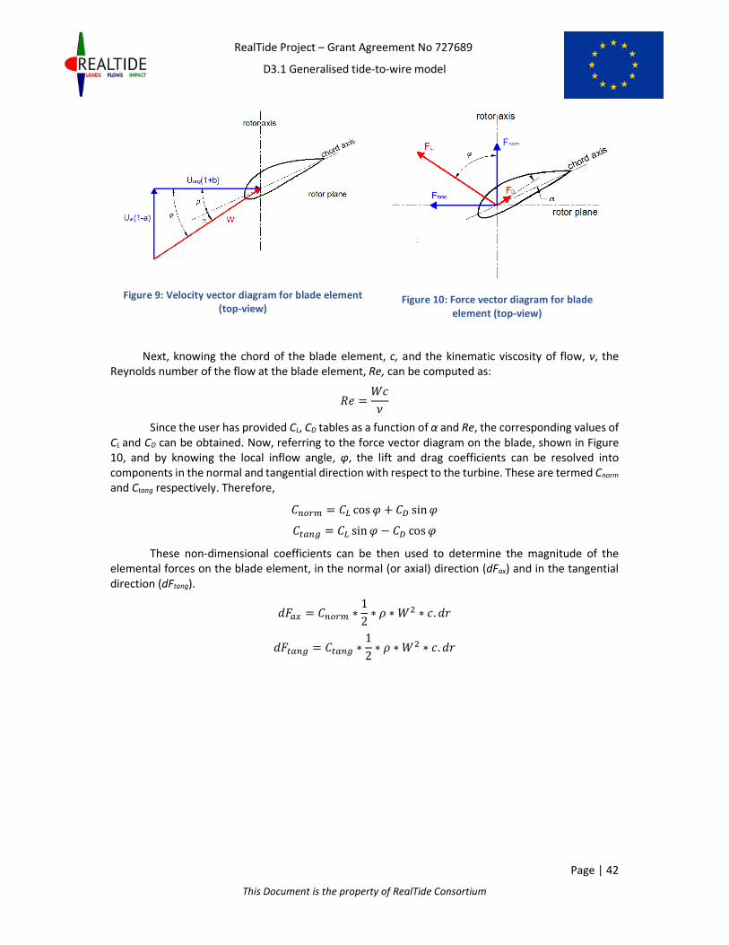
RealTide Project – Grant Agreement No 727689
D3.1 Generalised tide-to-wire model
Page | 42
This Document is the property of RealTide Consortium
Figure 9: Velocity vector diagram for blade element
(top-view) Figure 10: Force vector diagram for blade
element (top-view)
Next, knowing the chord of the blade element, c, and the kinematic viscosity of flow, ν, the
Reynolds number of the flow at the blade element, Re, can be computed as:
e: � t7x
Since the user has provided CL, CD tables as a function of α and Re, the corresponding values of
CL and CD can be obtained. Now, referring to the force vector diagram on the blade, shown in Figure
10, and by knowing the local inflow angle, φ, the lift and drag coefficients can be resolved into
components in the normal and tangential direction with respect to the turbine. These are termed Cnorm
and Ctang respectively. Therefore, M@y5z � M{ cos B G M| sin B Mv$@w � M{ sin B � M| cos B
These non-dimensional coefficients can be then used to determine the magnitude of the
elemental forces on the blade element, in the normal (or axial) direction (dFax) and in the tangential
direction (dFtang).
6$g � M@y5z ∗ 12 ∗ � ∗ t� ∗ 7. �
6v$@w � Mv$@w ∗ 12 ∗ � ∗ t� ∗ 7. �

RealTide Project – Grant Agreement No 727689
D3.1 Generalised tide-to-wire model
Page | 43
This Document is the property of RealTide Consortium
Figure 11: Front view of blade showing elemental forces
Here, dr is the span of the blade element in the radial direction. As can be seen from Figure 11,
this would depend on how fine the blade is segmented and this is the distance over which the blade
section, and its inflow velocity are assumed to be constant. However, since python has inbuilt
capabilities for numerical integration, this factor is not multiplied to the elemental force, and is kept
as the variable of integration.
The computation of elemental axial and tangential forces are done for each blade element on
each blade. The results are then to be integrated to obtain the total thrust and torque produced by
the turbine. The thrust produced by a single blade is given by:
�~��9b2h$���� � � 6$g==���
This integration is done within the code using in-built functions for numerical integration such
as Simpson’s integration rule or trapezoidal integration, with dr as the variable of integration. The total
thrust developed by the turbine would be the sum of the thrusts due to each blade. That is, if the
number of blades is nB,
�~��9b � � � 6$g==���
@s@��
Similarly, the torque generated by the turbine is the torque about the hub centre, due to the
tangential forces on the blade elements. Referring to Figure 11, this would be the moment due to all
elementary forces, dFtang about the blade centre. Therefore,
�8���: � � � �. 6v$@w==���
@s@��
The power generated by the turbine could be derived as the product of the torque and angular
velocity, ω in radians/second.

RealTide Project – Grant Agreement No 727689
D3.1 Generalised tide-to-wire model
Page | 44
This Document is the property of RealTide Consortium
�8�:� � �8���: ∗ V
It is usual to obtain these results in the form of non-dimensional coefficients in order to have
a better comparative figure. This is done by dividing the values with the force/torque/energy in the
incoming flow. For this purpose, a mean value of velocity is required, which here is the mean value of
the velocity profile across the blade diameter. Therefore, the Thrust Coefficient (CT), Torque Coefficient
(CQ) and Power Coefficient (CP) are defined as:
MN � �~��9b12 � ∗ �e� ∗ �z�$@�
M� � �8���:12 � ∗ �e# ∗ �z�$@�
MW � �8�:�12 � ∗ ��� ∗ �z�$@#
These computations are performed inside the Time loop. That is to say, they have to be
performed for each time step and for each TSR step. Outside the time loop, data can be extracted
showing the time history variation of these parameters. To plot the variation of these parameters with
TSR, the mean value over the given period of time for a given TSR can be calculated.
6.26.26.26.2 Shear Force & Bending Moment DistributionShear Force & Bending Moment DistributionShear Force & Bending Moment DistributionShear Force & Bending Moment Distribution
During the preliminary stage of design, it is important to analyze the strength of the blades and
the adequacy of the material reinforcement for the blades. Such kind of structural analysis is
performed by analyzing the shear force and bending moment distribution on the blades. The
elementary forces on each blade element, dFax and dFtang, are obtained as per the procedure
mentioned in Section 6.1. The blade is considered as a cantilever beam, fixed at its root, and subjected
to this force distribution. Therefore, the shear force and bending moment at any point along the length
of the blade can be found. For the explanations herewith, the computation of shear forces and bending
moment due to the axial force is only provided. This is the more significant part of the structural forces;
but, the same procedure can be followed for the tangential force as well.

RealTide Project – Grant Agreement No 727689
D3.1 Generalised tide-to-wire model
Page | 45
This Document is the property of RealTide Consortium
Figure 12: Distribution of forces, shear force and bending moment along blade length
A typical case of distribution of the axial force (dFax), the axial shear force (SFax) and the axial
bending moment (BMax) is shown in Figure 12. The origin of the graph is the hub centre of the turbine,
and the x-axis indicates the radial location along the blade. As can be seen, the shear force and bending
moment for the cantilever beam are zero at the tip of the blade, increasing towards a maximum value
at the root. The shear force is the difference between the cumulative integral of the force and the
reaction force at the root. The bending moment the cumulative integral of the shear force. Therefore,
at any point r from the hub centre, d6$g � e�`5yyv � � 6$g . �5=��� & ��$g � ��5yyv � � d6$g. �5=���
The reaction and bending moment at the root are the total integration of the forces along the
length of the blade. e�`5yyv � � 6$g . �=���=��� & ��5yyv � � d6$g . �=���=���
From a computational point of view, it would be easier to shift the origin to the tip of the blade,
so that a direct cumulative numerical integration can be applied to obtain these parameters. This
would be essentially transferring the forces from the co-ordinates system Xc-Yc to Xt-Yt in Figure 12.
Mathematically, this equivalency can be established by changing the variable of integration from r to
x, such that x = Rtip – r. The limits of integration also needs to be changed. When r = Rhub, x = Rtip – Rhub
and when r = Rtip, x = 0. Therefore, d6$g � � 6$g. �=����=���S & ��$g � � d6$g . �=����=���S
x Xc
Yc
Yt
Xt r
RealTide Project – Grant Agreement No 727689
D3.1 Generalised tide-to-wire model
Page | 46
This Document is the property of RealTide Consortium
It could be interesting to extend this result for computation of the thrust and torque of the
turbine as well. The thrust of the turbine is essentially the shear force calculated at its root. The torque
of the turbine needs a slight mathematical modification, since the moment needs to be calculated
about the hub centre.
�~��9b � � 6$g. �=���=���
� � 6$g . �=����=���S � ������
�8���: � � 6$g . �. �=���=���
� � � 6$g. �ev?� � ��. �ev?�=����=���
S
� ev?� � 6$g . �=����=���S � � 6$g . �. �=����=���
S � ����. ������ � � ����
6.36.36.36.3 Dynamic Stall ModuleDynamic Stall ModuleDynamic Stall ModuleDynamic Stall Module
As explained briefly in Section 3.5, the dynamic stall model employed in the python code is that
developed by Sheng for low Mach numbers [23]. This is a semi-empirical model, which means that the
equations within the model are not purely based on empirical or statistical relations; but they are
developed from an understanding of the physics of the phenomena. In line with this semi-empirical
approach, the entire solution for the dynamic stall problem is divided into different events
corresponding to those mentioned in Figure 7. The Sheng’s dynamic stall model is also implemented
with some modifications within the Matlab code developed by UEDIN, and details of this work is
available in [1]. The subsequent sections will explain the different phases of the dynamic stall, its semi-
empirical formulations and their applications in the Python code.
6.3.16.3.16.3.16.3.1 Solution in Attached FlowSolution in Attached FlowSolution in Attached FlowSolution in Attached Flow
This refers to the initial phase, wherein there is no separation of the flow around the aerofoil.
In this stage, the total lift coefficient is considered to be comprised of two components – a circulatory
component (CLc) which accounts for the circulation around the airfoil and a non-circulatory component
(CLnc) which accounts for flow acceleration effects.
When the vorticity of the airfoil is time varying, it is shed in the wake. This shed vorticity
induces a flow over the airfoil, so that the airflow sensed by the airfoil is not the free stream velocity
[33]. The shed wake causes a variation in the lift component when compared to an airfoil in a constant
stream velocity subjected to the same angle of attack. If the lift has been increasing for a while, then
vortices cause a downwash over the airfoil trailing edge, resulting in reduced lift. In the semi-empirical
dynamic stall model, this variation in lift is modelled as an effective lag in the angle of attack. The
equivalent angle of attack (αE) is determined by considering an indicial response function on the
incident angle of attack. Within the code, this is modelled in the form of two deficiency functions, X
and Y. For the time step n,
¡@ � ¡@��:�¢�£.¤> G ¥� ∗ �¦@ � ¦@��� ∗ :�¢�£.¤>�
§@ � §@��:�¢�£.¤> G ¥� ∗ �¦@ � ¦@��� ∗ :�¢�£.¤>�
where ¨9 � 2f$g¨b/7 is the non-dimensional reduced time.

RealTide Project – Grant Agreement No 727689
D3.1 Generalised tide-to-wire model
Page | 47
This Document is the property of RealTide Consortium
A1, A2, b1, b2, β are parameters that depend on the geometry of the aerofoil and can be determined
from wind tunnel test data for example. The lagged angle of attack, (αE) is obtained from the solution
for the angle of attack using static BEMT (α): ¦ª � ¦ � ¡ � §
The circulatory component of lift (CLc) is then found as M{3 � 2�¦ª. Alternatively, CL
c can also
be found from the lift coefficient database for an angle of attack of αE.
For calculating the non-circulatory lift coefficient, the Hansen approximation is used [36].
M{@3 � �7¦«2f$g , �~:�: ¦« � ¦@ � ¦@��
6.3.26.3.26.3.26.3.2 SeparatSeparatSeparatSeparation Pointion Pointion Pointion Point
This refers to Stage 2 of dynamic stall in Figure 7. To characterize this phenomenon, the
Kirchoff Theory [37] is used. This theory provides an equation relating the non-dimensional location of
the trailing-edge separation point (f), the static normal force coefficient (Cnorm), and the incident angle
of attack (α). This is given as:
M@y5z � M��¦ � ¦S� ®1 G H<2 ¯�
⇒ < � ±2 ∗ ² M@y5zM��¦ � ¦S� � 1³�
Figure 13: Trailing edge separation point as per Kirchoff theory [1]
Within the python program, a dataframe ‘Kirch’ is made for the computation of this separation
point. For any incident α, Cnorm can be computed as M@y5z � M{ cos B G M| sin B. Here, φ is the local
inflow angle, which is the sum of α and the twist angle, β (Figure 10). α0 is the angle of attack at which
the static lift coefficient is zero and CNα is the slope of the Cnorm vs α curve at this point of x-intercept.
These two parameters can be obtained from wind tunnel test data for the airfoil. Alternatively, they
can also be computed from the dataframe Kirch, since a tabular list of Cnorm vs α is available. With all
the other parameters known, f can be found from the equation above.
Applying the computations to the entire dataframe, one could obtain a lookup table
correlating a value of f for any α.

RealTide Project – Grant Agreement No 727689
D3.1 Generalised tide-to-wire model
Page | 48
This Document is the property of RealTide Consortium
6.3.36.3.36.3.36.3.3 Dynamic Stall OnsetDynamic Stall OnsetDynamic Stall OnsetDynamic Stall Onset
The onset of the dynamic stall occurs when the lagged angle of attack in the separated flow,
α’ exceeds a critical onset angle, αcr for the airfoil section. This depends on the reduced pitch rate, �« of
the aerofoil section in the unsteady flow. �« is defined as �« � « 3�´µ¶. Subsequently,
¦35 � · ¦�>S, �« ¸ �S¦>> G �¦�>S � ¦>>� �«�S , �« ¹ �S
αds0 = Critical dynamic stall onset angle in rad
αss = Angle of static stall in rad
r0 = Critical reduced pitch rate in rad
These values are also obtained from the wind tunnel test data. However, [23] noted that αds0
stays in the range of 17 to 18 degrees (0.297 to 0.314 rad) for many NACA aerofoils. In the same paper,
the value of r0 is also indicatively suggested as 0.01. αss can be also determined from the user input lift
coefficient data.
6.3.46.3.46.3.46.3.4 Separation Point LagSeparation Point LagSeparation Point LagSeparation Point Lag
Similar to the delay in angle of attack considered for attached flow (Section 6.3.1), there is a
delay in the case of separated flow also. This delay is modeled as a first order lag in the s domain, as
specified in [1]. Therefor, the delayed angle of attack, α’, is found using a deficiency function, Dα. For
the time step n, Dα is defined as:
º» � º»¼�:�¤>N½ G ¦ ∗« :�¤>�N½ ¦@ � ¦@ � º»
Here, Tα is an empirical time constant, which is also obtained from static wind tunnel test data.
Further, a delay shift from αss can be evaluated as:
¨¦� � · ¦�>S � ¦>>, �« ¸ �S�¦�>S � ¦>>� �«�S , �« ¹ �S
This delay shift of Δα1 from the static stall angle causes a delay in the separation point f. The
new effective angle of attack is given as ¦� � ¦′ � ¨¦�. Since a lookup table of f vs. α is available from
6.3.2, the delayed separation point (f’) corresponding to α2 could be obtained from this, i.e. < �<�¦��.
6.3.56.3.56.3.56.3.5 Vortex SheddingVortex SheddingVortex SheddingVortex Shedding
Once the dynamic stall has started, i.e.¦ ¸ ¦35, an additional lag occurs in the separation
point. This lag is modelled similar to the angle of attack lag in 6.3.1, using a deficiency function Dff
defined as follows:
º;;» � º;;»¼�:�¤>N¿ G �<@ � <@�� � ∗« :�¤>�N¿ < � < � º;;
Tv here is the vortex time constant, and is also one of the dynamic stall parameters determined
from tunnel tests. Within the python code, f’ is labelled as ff and f’’ is labelled as fff.

RealTide Project – Grant Agreement No 727689
D3.1 Generalised tide-to-wire model
Page | 49
This Document is the property of RealTide Consortium
Referring to Figure 7, at Stage 3, once there is an onset of dynamic stall, a vortex is generated
at the leading edge and this is convected further downstream with the flow. This vortex produces an
additional lift. In the Sheng’s model, this is modelled by a vortex shedding function (Vx), which is
parameterized in terms of a non-dimensional vortex passage time, τ. It is set to zero when there is
onset of dynamic stall (¦ ¸ ¦35�, and for the subsequent time steps it is incremented by the Δs value.
This increment continues until the foil starts pitching, i.e. when�« ¹ 0. Subsequently, τ is reset to zero,
and is re-initialized for the next instance of dynamic stall onset.
�g � ÀÁ 9Ã`#/� _ �Ä2�Åa , 0 ¹ Ä Æ �Å
789� _��Ä � �Å��Å{ a , Ä Ç �Å
6.3.66.3.66.3.66.3.6 Computation of NonComputation of NonComputation of NonComputation of Non----Linear Force coefficientsLinear Force coefficientsLinear Force coefficientsLinear Force coefficients
The final step of the dynamic stall module is to predict the force coefficients that would be
required to complete the thrust and torque calculations. Keeping in line with the same naming
conventions as for the static analysis in Section 6.1, the force coefficients parallel and perpendicular
to flow direction are referred as CD and CL respectively, and the force coefficients parallel and
perpendicular to the rotor axis direction as Cnorm and Ctang respectively (Figure 10). In addition, the force
coefficients parallel and perpendicular to the chord axis are referred as CCu and CN
u respectively. The
definition of CCu and CN
u follows the same as used in [1].
M�È � M{3 É1 G H<′′2 Ê Type equation here. 2 G M{@3 G M�Å
CLc = circulatory component of lift from attached flow solution in 6.3.1
CLnc = non-circulatory component of lift from attached flow solution in 6.3.1
CNv = vortex lift component from 6.3.5 = B*(f’’-f)*Vx
B = dynamic stall parameter
Also, M&È � ÔM��¦ª � ¦S��RH<′ � ÕST
α0 = angle of attack at which static CL equals zero
αE = equivalent angle of attack from attached flow solution in 6.3.1
CNα = slope of the Cnorm vs α curve at α0 as defined in 6.3.2
E0 = dynamic stall parameter
Thereafter, the lift and drag coefficients can be computed by resolution of the forces. M{ � M�È cos ¦ G M&È sin ¦ M| � M�È sin ¦ � M&È cos ¦ G M|S
CD0 = static drag coefficient at α0
The equation for CD can also be replaced by the one given by [38]. Therfore, M| � M|>v G M|?@� G M|Å?>

RealTide Project – Grant Agreement No 727689
D3.1 Generalised tide-to-wire model
Page | 50
This Document is the property of RealTide Consortium
CDst = static drag coefficient determined from static BEMT
CDind = CL (α – αE)
M|Å?> � �M|>v � M|S� ÖÉ1 G H<′′2 Ê� � ®1 G H<�¦ª�2 ¯�×
Subsequently, the normal and tangential components can be evaluated the same way as was
done for static BEMT. The computation of the elementary forces and the subsequent calculations
follow the same procedure as well. M@y5z � M{ cos B G M| sin B Mv$@w � M{ sin B � M| cos B

RealTide Project – Grant Agreement No 727689
D3.1 Generalised tide-to-wire model
Page | 51
This Document is the property of RealTide Consortium
7777 PRE PROCESSOR PRE PROCESSOR PRE PROCESSOR PRE PROCESSOR –––– USER INTERFACEUSER INTERFACEUSER INTERFACEUSER INTERFACE
Although the software developed is not comprehensively designed for commercial use, the
presence of a user interface enhances the usability of the code. The prime focus of the work is the
development of a functional tool; but a considerable sight has also been given into the development
of a user-friendly interface. Managing and modifying input variables within the Python code is not only
cumbersome, but also can lead to undesirable outputs and malfunctioning of the program. Moreover,
the code is expected to be used in the future by users who are not familiar with the development.
Hence it is always advisable to disseminate only the relevant information to the user.
Giving due consideration to all these factors, a simple user-interface was developed using the
Python Tkinter library. A snapshot of this is shown in Figure 14. This library generates a graphical user
interface based on predefined widgets, such as buttons, labels, checkbuttons, radiobuttons etc., and
by placing them on a grid oriented framework.
Figure 14: Graphical User Interface for the Python code
During the design of the user interface, various user input variables and possible scenarios of
usage of the tool were analyzed. Subsequently, the following parameters were identified as critical
user input values:
1) Geometry of the tidal turbine
2) Input velocity profile
3) Operating conditions of the tidal turbine
4) Various BEMT improvements that need to be considered in the analysis

RealTide Project – Grant Agreement No 727689
D3.1 Generalised tide-to-wire model
Page | 52
This Document is the property of RealTide Consortium
7.17.17.17.1 Geometry of the tidal turbineGeometry of the tidal turbineGeometry of the tidal turbineGeometry of the tidal turbine
The requirement for reusability of the code for different tidal turbines would mean that the code
should be able to accept and use different blade geometry data. Typically this would include the key
geometrical parameters, the shape of the blades and the lift and drag coefficients of the aerofoil
sections used in the blade. The term aerofoil sounds like a misnomer for a tidal environment; however,
the same is used throughout the code, without any loss in generality.
7.1.17.1.17.1.17.1.1 Key GeometrKey GeometrKey GeometrKey Geometrical Parametersical Parametersical Parametersical Parameters
Figure 15: Window for entry of geometrical data
The key geometrical parameters that define the tidal turbine are the number of blades, its
diameter (or radius), radius of the hub and its pitch. These parameters are accepted through the ‘Input
Blade Geometry’ button in the ‘Blade Data’ section. A screenshot of the pop-up window which accepts
these geometric inputs is shown in Figure 15. This section also accepts the input of various
environmental factors such as the density and viscosity of the fluid. Default values and units are loaded
into the code, so that the user is aided with a reference.
7.1.27.1.27.1.27.1.2 Shape of the BladesShape of the BladesShape of the BladesShape of the Blades
The shape of the blades is defined by the radius, chord and thickness at different locations along
its length. To accurately define the geometry multiple sections are used usually. This would make it
cumbersome for the user to enter it all within the user interface. Hence, these values are accepted in
a tabular format (.csv) using the ‘Load Geometry Data’ button shown in Figure 15. When loaded, the

RealTide Project – Grant Agreement No 727689
D3.1 Generalised tide-to-wire model
Page | 53
This Document is the property of RealTide Consortium
table displaying the geometrical shape of the blades is updated to give the user an indication of the
values entered and to verify it. An image or plot showing the blade geometry could also be added later
on as a feature, so that the user has a visual representation of the blade geometry, and can be aware
of any possible mistakes in the entry.
For simplicity, the geometrical sections entered by the user are used for BEMT computations. That
is to say, the calculations are performed at each of these radial locations, and the results integrated to
find the total force on the blade. For this reason, the user needs to be aware that even though more
number of sections accurately define the geometry, this would also require the program to compute
the solution at each of these sections, and consequently increase the overall computation time. The
user needs to input the number of blade sections accordingly. The number of blade element sections
(n) are updated in the main window, as can be seen in Figure 14.
7.1.37.1.37.1.37.1.3 Lift and Drag coefficients of the aerofoil sectionsLift and Drag coefficients of the aerofoil sectionsLift and Drag coefficients of the aerofoil sectionsLift and Drag coefficients of the aerofoil sections
The performance of the blades depend on the type of aerofoil sections that are used in the blades.
The blade shape parameters only define the maximum thickness at the particular radial location; but
its lift and drag performance depends on the particular aerofoil section that is used at this location.
Typically these are standard NACA profiles, with their performance specified by tables of lift and drag
coefficients (CL and CD respectively).
Calculation of CL and CD from the geometry of the blade is not an advisable method due to the
possibility of having inaccurate data. These being standard NACA profiles, the static CL and CD values
are usually available as experimental results or from CFD analysis. By clicking the ‘Input Lift and Drag
Coefficients’ button in the ‘Blade Data’ section, the user can input such tables of CL and CD.
For complex turbine geometries, it is possible to have multiple NACA profiles along the length of
the blade. However, these may not coincide with the blade element sections as previously entered by
the user. Also, the number of NACA segments within the blade geometry are usually much lesser than
the number of blade element sections required for computation. For these reasons, the number of
NACA segments is taken as a different variable input from the user, under the heading ‘Number of
blade segments [m]’, as can be seen in Figure 14. Based on this number, the popup window for ‘Input
Lift and Drag Coefficients’ will have the corresponding number of columns for user input of CL and CD.
A representation of this window for number of blade segments equal to 2 is shown in Figure 16. In
order to educate the user about the difference between the ‘Number of blade element sections [n]’
and ‘Number of blade segments [m]’, an info button is provided, which produces a diagram explaining
the difference between the two. A snapshot of this diagram is provided in Figure 17.
The input file for CL and CD is entered as a csv table of values. The first column contains the list of
angle of attacks (α). The first row contains the list of Reynolds Numbers (Re). CL and CD are each entered
then as functions of α and Re. The user also needs to associate each lift and drag coefficient database
to the corresponding geometrical location on the blade. This is done by entering the ‘Start of Section’
value in the window shown in Figure 16. The start of the initial segment is taken as the radius of the
hub, by default.

RealTide Project – Grant Agreement No 727689
D3.1 Generalised tide-to-wire model
Page | 54
This Document is the property of RealTide Consortium
Figure 16: Window for entry of Lift and Drag
coefficients
Figure 17 : Information about blade elements and
blade segments
In normal operation, the lift and drag data available for aerofoil sections do not cover their
possible 360 degree. However, for the dynamic stall calculations, in some cases the angles can be very
high, and the program needs the corresponding CL and CD values to perform computations at these
cases. Also, since the BEMT solution is an iterative approach, it could be possible that during the
iterative process, the angle of attack during an iteration goes to a very high value, and then converges
to the actual angle of attack. To ensure that such convergence occurs, the database for CL and CD has
to have a range from -180o to +180o. An inbuilt feature has been developed in the code, that
extrapolates the lift and drag to this complete range, in case it is not available. This extrapolation is
based on Viterna extrapolation method, which is mentioned in [5]. A graphical indication of this
extrapolation process is indicated in Figure 18, where the blue * indicates the data originally entered
by the user and the red dotted lines represent the extrapolated data.
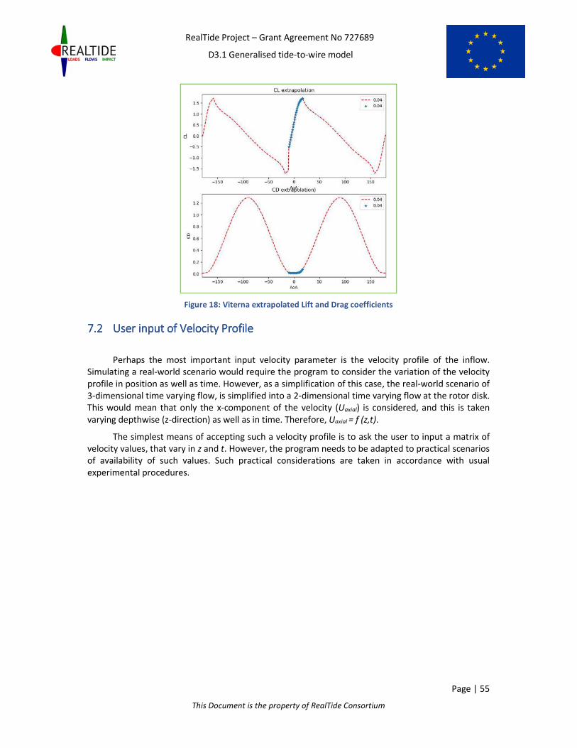
RealTide Project – Grant Agreement No 727689
D3.1 Generalised tide-to-wire model
Page | 55
This Document is the property of RealTide Consortium
Figure 18: Viterna extrapolated Lift and Drag coefficients
7.27.27.27.2 User input of Velocity ProfileUser input of Velocity ProfileUser input of Velocity ProfileUser input of Velocity Profile
Perhaps the most important input velocity parameter is the velocity profile of the inflow.
Simulating a real-world scenario would require the program to consider the variation of the velocity
profile in position as well as time. However, as a simplification of this case, the real-world scenario of
3-dimensional time varying flow, is simplified into a 2-dimensional time varying flow at the rotor disk.
This would mean that only the x-component of the velocity (Uaxial) is considered, and this is taken
varying depthwise (z-direction) as well as in time. Therefore, Uaxial = f (z,t).
The simplest means of accepting such a velocity profile is to ask the user to input a matrix of
velocity values, that vary in z and t. However, the program needs to be adapted to practical scenarios
of availability of such values. Such practical considerations are taken in accordance with usual
experimental procedures.

RealTide Project – Grant Agreement No 727689
D3.1 Generalised tide-to-wire model
Page | 56
This Document is the property of RealTide Consortium
Figure 19 : Conventional experimental set-up for performance evaluation of tidal turbines
Figure 19 shows a typical experimental set-up. Sensors are placed on the blades of the turbine
to measure the strain on them and the rotor thrust. Also, the measurement of the rotor torque is done
by sensors on the nacelle. The velocity measurements are taken using a flow velocity sensor, placed at
a distance D in the downstream direction of the flow. This velocity sensor could be an Acoustic Doppler
Current Profiler (ADCP), which generates sound waves to the bottom of the surface and characterises
the velocity at different points based on the doppler shift of the returning waves [30]. Having a multi-
beam ADCP would allow for velocity measurements at different points along the depth; otherwise the
velocity variation with time at a single point is obtained.
The usual procedure is to obtain the velocity (Vref ) at the sensor location (zref ) and then
extrapolate it to the depth of the tank using a power law. The power law depends on the depth of the
tank, and it assumes zero velocity at the bottom of the basin (no slip boundary condition), with a power
variation for increasing z. The corresponding velocity (V) at any point (z) is given in terms of a power
factor (pf) as:
� � �5�; ∗ ® [[5�;¯�;
Now, the input from the user would be the reference velocity, Vref. This can be a constant value
(in case of steady flow) or a time varying flow. In case the depth-wise variation is to be considered, the
user also provides the power factor, and the code extrapolates the velocity data along the depth. For
a constant velocity input, the input window that appears is as shown in Figure 20. In the case that the
velocity input is time varying, then the user needs to specify a file in .csv format, which includes Vref as
a function of time.

RealTide Project – Grant Agreement No 727689
D3.1 Generalised tide-to-wire model
Page | 57
This Document is the property of RealTide Consortium
Figure 20: User input of velocity parameters (constant velocity)
As could be seen from Figure 15, the code can take velocity inputs from environmental
conditions instead of experimental measurements (see Figure 21). This part of the program is meant
for it to be useful for classification purposes. The velocity definitions used here are in accordance with
Bureau Veritas classification guidelines for current and tidal turbines, NI 603 [27]. Presently, the code
only adds the current velocities due to tides, winds and waves, and considers that as a constant stream
velocity. The input window is the same as Figure 20, but with the value of predefined from the previous
window. However, during improvement of the code, additional features to calculate the current
velocity from tide height, wind speed and wave height could be developed.
Figure 21: Velocity input as per NI603

RealTide Project – Grant Agreement No 727689
D3.1 Generalised tide-to-wire model
Page | 58
This Document is the property of RealTide Consortium
7.37.37.37.3 Definition of Rotation SpeedDefinition of Rotation SpeedDefinition of Rotation SpeedDefinition of Rotation Speed
The operating profile of the turbine is defined by a combination of the inflow velocity and the
turbine rotation speed. This is characterized by indicating a Tip-Speed Ratio (TSR), which is the ratio
between the angular velocity at the tip of the blades to the inflow axial velocity.
However, in the BEMT tool, the rotation speed is characterized not by the TSR, but instead by
the RPM of the turbine. This is mainly owing to the dynamic nature of both the inflow velocity and the
rotation speed. When both are dynamically varying with time, it is meaningless to define an arbitrary
tip-speed ratio to characterize the operating condition. Hence, the input of the rotation speed is taken
separately. The various options for rpm input can be seen from Figure 14. These are:
a) Constant RPM
b) Varying RPM (experimental measurements)
c) Multiple RPM
d) RPM as feedback
Similar to the inflow velocity, the rotation speed can also be a constant value or varying value.
In case of a constant value, the user enters the same in an entry box provided. A dynamically varying
rpm value is usually obtained as experimental measurement, from the sensors on the blades in Figure
19. Such input needs to be provided in csv format. It is pertinent to mention that the time steps for the
velocity variation and rpm variation need not be the same. The code interpolates the value of rpm for
the same time stamp as that of the velocity input.
It is an usual scenario for the user to perform the BEMT analysis for multiple rotation speeds
(multiple TSRs). Instead of running the code multiple times with a constant rpm input, the program
provides the user an option to enter all these rpm values in a tabular csv format.
The last option for the rpm input is to enter rpm as feedback. This part refers to the integration
with the electrical module.
7.47.47.47.4 Selection of BEMT Improvement modulesSelection of BEMT Improvement modulesSelection of BEMT Improvement modulesSelection of BEMT Improvement modules
Finally, the user needs to select the BEMT improvement modules that need to be considered
during the course of the analysis. These improvements are the same as mentioned in Section 3.
A modular approach is followed for the implementation of these functions. That is to say, each
module acts as an optional plug-in, which are activated only if the corresponding check-box in the user
interface is checked.
It might also be noted that some of these improvements have cross-links between each other. For
example, the correction for high-induction factor is included within the BEMT solver algorithm. This
means that the corresponding functions need to be defined for both the iterative algorithm as well as
single-variable parametrization algorithm. Presently, the modules for dynamic wake and rotational
augmentation are not completely implemented and validated; and hence, they are greyed out in Figure
14. It is also pertinent to mention that the list of improvements is non-exhaustive, and any additional
modules may be directly linked to the user-interface in the form of check-buttons or radio-buttons.

RealTide Project – Grant Agreement No 727689
D3.1 Generalised tide-to-wire model
Page | 59
This Document is the property of RealTide Consortium
8888 POST PROCESSINGPOST PROCESSINGPOST PROCESSINGPOST PROCESSING
One factor which probably has a large bearing on the usefulness of a computer program is the
manner in which the output is made available to the user. The basic aim for developing such codes is
to reduce human effort in computation and access results in a convenient and most direct manner
possible. For these reasons, it is necessary to identify the output requirements, design an interface to
efficiently access these, and implement a framework that can be used to build on for future inclusions.
The code is intended to be utilized during the preliminary design phase. This is the design
validation phase, where the designer needs access to the dependency of certain key parameters with
changes in some of the design variables. Primarily, this would be in the form of plots that would benefit
the designer by providing a visual indication of the influence of the design variables. The quantum of
such possible dependencies are quite large at this stage of the design, and hence it is not possible to
pinpoint definitively on a desired output format.
Moreover, the computational data processed during the execution of the program is also huge.
The program performs computations for different blade elements, different blades, different
operating conditions, different time steps, and using different algorithms. The program does not retain
all of these data, as this also has an effect on the computational speed. A good understanding about
the scope of different variables is desired to make sure that only the relevant variables are present
within the workspace.
All these reasons call for a well-structured data management system, that allows the user to
access the desired variables. Even though such detailed planning is only required for highly complex
codes, a preliminary implementation of such a concept at this stage would be beneficial for future
developments. Accordingly, a hierarchy of dictionaries for storing the results is conceived, and stored
in a single dictionary variable named ‘Results’. The schema of the nested dictionary variable is shown
in Figure 22.
Referring to Figure 22, the final output is stored at 4 different dictionary levels within the
hierarchy. These are Results level, TSR level, Blade level, and Blade element level in descending order
of data storage levels. Each level is characterized by dictionaries of output data, which further contain
data pertaining to their sub-levels.

RealTide Project – Grant Agreement No 727689
D3.1 Generalised tide-to-wire model
Page | 60
This Document is the property of RealTide Consortium
Figure 22: Hierarchy of ‘Results’ variable
Within the ‘Results’ variable, the results for each operating condition are stored. This is indicated
by TSR = i_TSR in Figure 22. Within each of the operating condition, the global results for the force
computations are stored. These parameters are typically the thrust, torque and power generated by
the turbine, and their associated dimensionless coefficients (CT, CQ and CP respectively). As these
parameters are for the entire turbine, they are termed as global results. They are stored as arrays for
the entire time duration. These results are available for both the static and dynamic cases; however
the schematic shows the branching only for the static case for the sake of simplicity. A time-average
of these results is available directly under the ‘Results’ variable, at the Results level.
Also available at the TSR level are the dictionaries for each blades. Figure 22 shows only one of
these, indicated by Blade ‘N’. In reality, there would be a dictionary variable corresponding to each
blade of the turbine. The results that can be extracted from the Blade dictionary are the shear forces
and bending moment distributions along its length. The Blade dictionary also has sub-dictionaries for
each Blade element on it. These are indicated as Blade element ‘j’ in the schematic. The Blade element
dictionaries include the results from the iterative BEMT computations (static BEM parameters) and the
results from the Dynamic Stall module (Dynamic Stall results). The results from the computation of the
elemental forces on the blade element are also included at this level.
Once the storage of results is established, as shown in Figure 22, a study on the various forms
of output required by the user needs to be undertaken. As stated earlier, this would primarily be in the

RealTide Project – Grant Agreement No 727689
D3.1 Generalised tide-to-wire model
Page | 61
This Document is the property of RealTide Consortium
form of plots between a dependant variable (x) and an independent variable which is the desired
output (y). The subsequent sections analyze the possibilities within this framework.
8.18.18.18.1 Independent variablesIndependent variablesIndependent variablesIndependent variables
8.1.18.1.18.1.18.1.1 TSRTSRTSRTSR
During the preliminary design process, it is usual to come across situations where the optimum
operating speed of the turbine for a given inflow condition needs to be determined. Within the BEMT
code, such an analysis can be performed using the multiple rpm input option. In such design scenarios,
it would be useful to plot the variation of parameters against the operating TSR of the turbine.
In a TSR based output analysis, the output that required to be analysed could be the force parameters.
This would include the variation of thrust, torque, power and/or the associated non-dimensional
coefficients with TSR. Also of interest to the designer, from a structural point of view, would be the
root bending moment at each blade. In a dynamic analysis, the designer could be interested in the
average value, mean value or maximum value of either of these parameters.
8.1.28.1.28.1.28.1.2 TimeTimeTimeTime
A dependency on time is usually preferred when performing a dynamic analysis. The variation of
various parameters as a function of time would be required to be plotted. The dependant variable (y)
could be the same as that mentioned for the TSR case. However, here instead of a time-average, the
evolution of the quantity as a function of time needs to be plotted.
8.1.38.1.38.1.38.1.3 Along length of bladeAlong length of bladeAlong length of bladeAlong length of blade
Another possible form of output requirement would be the plotting of forces along the length of the
blade. Such parameters are typically required for a strength analysis of the blade. The parameters that
can be plotted as a function of the length along the blade are the shear force, bending moment,
elementary axial forces and elementary tangential forces. The shear force and bending moment
distribution is obtained from the computations performed as per Section 6.2. The elementary forces
are computed by BEMT for each blade element, and these can also be plotted to analyse the force
distribution. Typical plots pertaining to the length of the blade are the same as seen in Figure 12. Since
these computations are performed for each TSR and each time step, input parameters need to be
taken from the user which specify these.
8.28.28.28.2 Relational hierarchyRelational hierarchyRelational hierarchyRelational hierarchy
Since there are multiple possibilities for plotting the output, it would beneficial to establish a relational
hierarchy between the parameters involved. A mapping between the independent variables (x) and
the dependent variables (y) is made, as shown in Figure 23. Such a mapping is also extended to the
post-processing GUI, wherein when the user selects a parameter for x, the table for y updates
automatically to show only the relevant output options.
The relational mapping in Figure 23 indicates the mapping from x to y, with the possible optional
parameters indicated in rectangular boxes on the right. It could be seen that there are 6 possible
combinations for output that need to be taken into account. These are TSR-Forces, TSR-RBM, Time-
Forces, Time-RBM, Length-Shear Force and Length-Bending Moment. This would mean that the code
would need to define 6 different functions to handle each of these scenarios.

RealTide Project – Grant Agreement No 727689
D3.1 Generalised tide-to-wire model
Page | 62
This Document is the property of RealTide Consortium
Figure 23: Relational mapping for output variables
Additionally, some of these output plots would require optional input from the user. For example,
while plotting force or RBM against TSR, the value that corresponds to each TSR could be the mean
value from the dynamic analysis, or the maximum value or the minimum. The same is also applicable
while plotting Shear Force and Bending Moment. Alternatively, this can also correspond to a particular
instant of time.
Similarly, while plotting results for dynamic analysis (Force vs Time etc.), the particular operating
condition for which the result needs to be plotted (TSR = ?), needs to be specified by the user. While
plotting blade related data, the user should have the option for selecting the blades for which he wants
to plot the results. When plotting the forces, he should also be able to choose the type of parameter
he wants to plot – Thrust, Torque, Power, CT, CQ or CP.
The mapping shown in Figure 23 is non-exhaustive. When adding additional output options, they
can be included within this diagram to give an idea to the programmer as to what are the additional
functions required to define and what are the relations that need to be modified. Such a mapping is
included because it is expected that the requirement for various post-processing options is expected
to increase as the tool gets used more. Having such a fundamental structure for the post-processing
code, makes it easier to modify the code.
Some other possible output options that could be included are the plotting of elementary axial
and elementary tangential forces, along the length of the blade. Also, the user might be interested in
analyzing the impact of the input variables on the output results. So, it could also be possible to include
plotting of the operating conditions, such as inflow velocity and rotation speed (or TSR). A screenshot
of the post-processing GUI is shown in Figure 24. The output options that are available are also
illustrated with an example in Figure 25 for the case when TSR and Forces are selected by the user.

RealTide Project – Grant Agreement No 727689
D3.1 Generalised tide-to-wire model
Page | 63
This Document is the property of RealTide Consortium
Figure 24: Postprocessing GUI window
Figure 25: Postprocessing output options
The code is also developed in such a way that the relevant output files are saved in csv format. The
folder location for this is kept as the same location from where the user inputs the geometry data.
Currently, the output csv files generated are the time history variations of the force parameters (static
BEMT and dynamic stall), as well as the variation of the mean values of these parameters with the TSR.
These can be supplemented in the future as per requirement.

RealTide Project – Grant Agreement No 727689
D3.1 Generalised tide-to-wire model
Page | 64
This Document is the property of RealTide Consortium
9999 VALIDATION CASE STUDVALIDATION CASE STUDVALIDATION CASE STUDVALIDATION CASE STUDIESIESIESIES
Development of any numerical code is associated with its validation as well. Such codes
implement theoretical models to simulate real-world scenarios, and its accuracy and suitability needs
to be validated with more accurate results. For the case of the python BEMT tool, such validation cases
could be experimental tests, sea trials, or CFD analysis. With a research on existing literature on the
subject, valid test cases could be obtained.
Being a relatively new industry, there are not many test cases available within the tidal turbine
industry, especially for the dynamic analysis. However, the application of BEMT is the same in the case
of wind turbines as well. The fluid mechanics of the operating scenario is the same, with the change
only in the fluid environment. Moreover, the amount of experimental research conducted in the
aerodynamic industry, particularly for wind turbines, is much more. Many of the commercial tidal
turbine codes have also used wind turbine data for validation. Hence, the use of such data is also
considered for the validation process.
4 different test cases are chosen for the validation of the BEMT tool. The static and dynamic BEMT
modules are validated separately. The validation of the combined tool would require experimental
tests and measurements designed for this specific purpose. For the validation of static BEMT,
experimental measurements on marine current turbines by Bahaj, CFD results for Hobit tidal turbine,
and the results on Sabella D10 tidal turbine are used as benchmarks. To validate the dynamic stall
module, the wind tunnel test data for a single aerofoil subjected to sinusoidally varying pitching motion
is used. This section describes more about each of these test cases and the comparison of the results
obtained.
It must also be mentioned that during the actual development phase, many more validation case
studies were conducted. However, these 4 case studies are indicative about the extent of validation
that has been conducted. Other cases that were considered were of similar input characteristics and
hence omitted for brevity.
9.19.19.19.1 BahajBahajBahajBahaj
The experimental measurements done by Bahaj was performed on a 800mm diameter model
turbine in a cavitation tunnel and a towing tank [39]. Measurements of shaft power and thrust
generated by the turbine are made for a series of blade pitch settings and speeds. The turbine consists
of 3 blades, and the experimental set-up is shown in Figure 26.
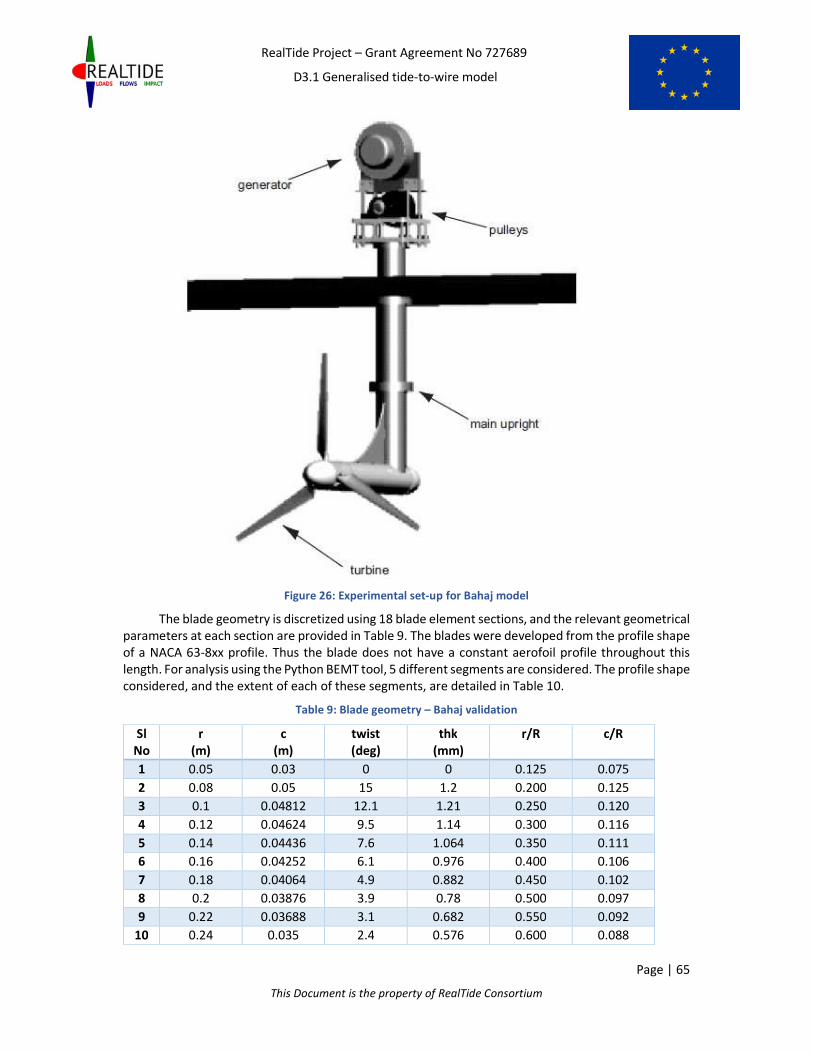
RealTide Project – Grant Agreement No 727689
D3.1 Generalised tide-to-wire model
Page | 65
This Document is the property of RealTide Consortium
Figure 26: Experimental set-up for Bahaj model
The blade geometry is discretized using 18 blade element sections, and the relevant geometrical
parameters at each section are provided in Table 9. The blades were developed from the profile shape
of a NACA 63-8xx profile. Thus the blade does not have a constant aerofoil profile throughout this
length. For analysis using the Python BEMT tool, 5 different segments are considered. The profile shape
considered, and the extent of each of these segments, are detailed in Table 10.
Table 9: Blade geometry – Bahaj validation
Sl
No
r
(m)
c
(m)
twist
(deg)
thk
(mm)
r/R c/R
1 0.05 0.03 0 0 0.125 0.075
2 0.08 0.05 15 1.2 0.200 0.125
3 0.1 0.04812 12.1 1.21 0.250 0.120
4 0.12 0.04624 9.5 1.14 0.300 0.116
5 0.14 0.04436 7.6 1.064 0.350 0.111
6 0.16 0.04252 6.1 0.976 0.400 0.106
7 0.18 0.04064 4.9 0.882 0.450 0.102
8 0.2 0.03876 3.9 0.78 0.500 0.097
9 0.22 0.03688 3.1 0.682 0.550 0.092
10 0.24 0.035 2.4 0.576 0.600 0.088

RealTide Project – Grant Agreement No 727689
D3.1 Generalised tide-to-wire model
Page | 66
This Document is the property of RealTide Consortium
Sl
No
r
(m)
c
(m)
twist
(deg)
thk
(mm)
r/R c/R
11 0.26 0.03312 1.9 0.494 0.650 0.083
12 0.28 0.03124 1.5 0.42 0.700 0.078
13 0.3 0.02936 1.2 0.36 0.750 0.073
14 0.32 0.02752 0.9 0.288 0.800 0.069
15 0.34 0.02564 0.6 0.204 0.850 0.064
16 0.36 0.02376 0.4 0.144 0.900 0.059
17 0.38 0.02188 0.2 0.076 0.950 0.055
18 0.4 0.02 0 0 1.000 0.050
Table 10: Blade segments – Bahaj validation
Segment
No
Radial Span
(m to m)
t/c Aerofoil profile
0 0.05 to 0.08 0.24 NACA 63824
1 0.08 to 0.12 0.21 NACA 63821
2 0.12 to 0.18 0.18 NACA 63818
3 0.18 to 0.30 0.15 NACA 63815
4 0.30 to 0.40 0.12 NACA 63812
The validation is done for a test case of 5 degrees pitch and an inflow velocity of 1.7m/s. 5
different operating conditions (or rotation speeds) are chosen for the study. The tip-speed ratio (TSR)
and the rotation speed in revolutions/min (RPM) are tabulated in Table 11. The results from the CFD
analysis usin STAR-CCM+ is also available for these 5 conditions. Also available are the results from the
Matlab BEM code developed by Hydrocean. The objective of this validation study will be to compare
the results of the non-dimensional coefficients for thrust (CT), torque (CQ) and power (CP) from the 4
different tools.
Table 11: List of operating conditions – Bahaj validation
TSR RPM
4.5 182.63
5.5 223.21
6.5 263.8
7.5 304.38
8.5 344.97
The results from the validation study are presented in Figure 27. The non-dimensional
coefficients for thrust, torque and power (CT, CQ, and CP respectively) have been graphically compared
for the BEMT tool in Python, CFD analysis and the results presented in the work by [39], for a TSR range
from 4.5 to 8.5. As can be seen, the results from the BEMT tool (Python BEM red curve) are in good
agreement with both the benchmark test results.

RealTide Project – Grant Agreement No 727689
D3.1 Generalised tide-to-wire model
Page | 67
This Document is the property of RealTide Consortium
Figure 27: Comparison of CT, CQ, and CP - Bahaj validation
9.29.29.29.2 Sabella D10Sabella D10Sabella D10Sabella D10
The second validation case is also that for a tidal turbine. Here, the D10 tidal turbine of Sabella
is used for the analysis. Figure 28 shows an image of this turbine. It is a 6-bladed turbine with an overall
diameter of 9.85m. The hub radius is 1.925m. The blade is discretized into 12 sections. The turbine has
a constant section throughout its length, with a constant chord. The section is elliptical and its
aerodynamic performance parameters are available from wind tunnel tests. The geometry details are
not provided for confidentiality purposes.
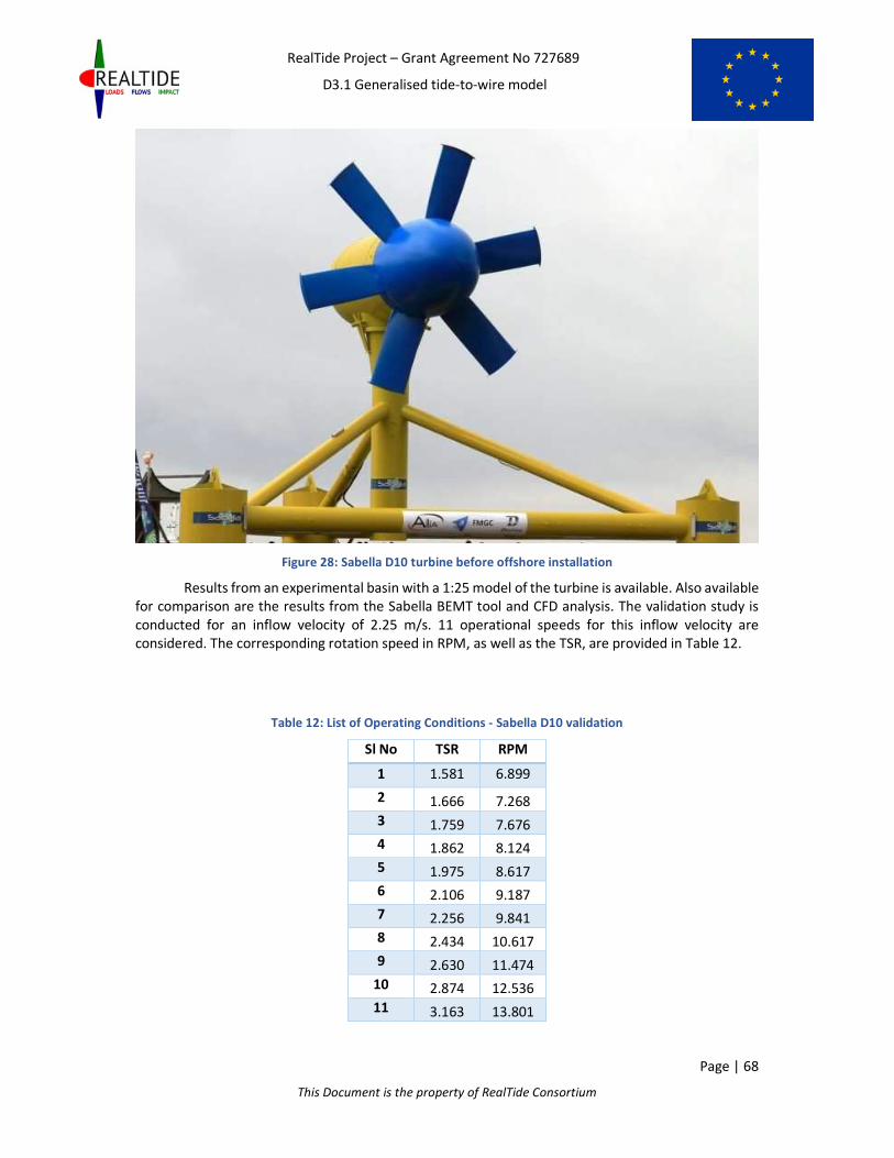
RealTide Project – Grant Agreement No 727689
D3.1 Generalised tide-to-wire model
Page | 68
This Document is the property of RealTide Consortium
Figure 28: Sabella D10 turbine before offshore installation
Results from an experimental basin with a 1:25 model of the turbine is available. Also available
for comparison are the results from the Sabella BEMT tool and CFD analysis. The validation study is
conducted for an inflow velocity of 2.25 m/s. 11 operational speeds for this inflow velocity are
considered. The corresponding rotation speed in RPM, as well as the TSR, are provided in Table 12.
Table 12: List of Operating Conditions - Sabella D10 validation
Sl No TSR RPM
1 1.581 6.899
2 1.666 7.268
3 1.759 7.676
4 1.862 8.124
5 1.975 8.617
6 2.106 9.187
7 2.256 9.841
8 2.434 10.617
9 2.630 11.474
10 2.874 12.536
11 3.163 13.801

RealTide Project – Grant Agreement No 727689
D3.1 Generalised tide-to-wire model
Page | 69
This Document is the property of RealTide Consortium
Figure 29: Comparison of CT, CQ, CP - Sabella D10 validation
The results from the validation study are plotted in Figure 29, Python BEM is the red curve. As
can be seen, the results for the torque and power coefficients (CQ and CP) have a good relation across
the different tools. However, there is a discrepancy in the thrust coefficient (CT). The model testing and
CFD analysis show a high value of CT compared to both BEMT tools. Further investigation is required
into this. Some critical analysis of the same is provided in the subsequent paragraphs.
One of the disadvantages of the tip and hub loss modules implemented within the BEMT tool is
that they are arbitrarily defined, only based on the dimensions of the blades. Performance enhancing
design features such as the presence of a winglet at the blade tip, or the aerodynamic shape of the
hub are not considered when defining these factors. As can be seen in Figure 28, the D10 turbine
incorporates both these features. Accordingly, the tip and hub losses would not be as high as that
predicted by BEMT.
To ascertain this supposition, another BEMT analysis with the Python tool was conducted,
without considering any tip and hub losses. The results are plotted in Figure 30. It could be noted that
the results are in better agreement with the CFD results. It was also found from the CFD analysis that
a difference of 5% in CT could be attributed to the hub drag. BEMT does not consider this drag effect.
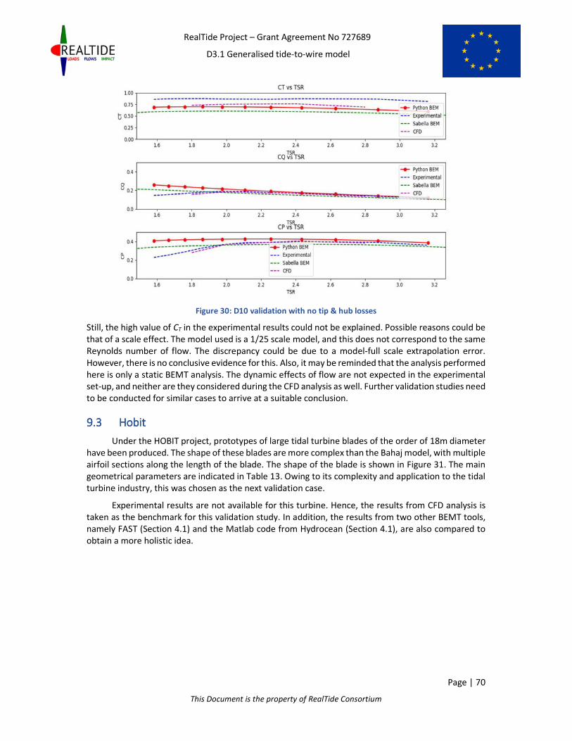
RealTide Project – Grant Agreement No 727689
D3.1 Generalised tide-to-wire model
Page | 70
This Document is the property of RealTide Consortium
Figure 30: D10 validation with no tip & hub losses
Still, the high value of CT in the experimental results could not be explained. Possible reasons could be
that of a scale effect. The model used is a 1/25 scale model, and this does not correspond to the same
Reynolds number of flow. The discrepancy could be due to a model-full scale extrapolation error.
However, there is no conclusive evidence for this. Also, it may be reminded that the analysis performed
here is only a static BEMT analysis. The dynamic effects of flow are not expected in the experimental
set-up, and neither are they considered during the CFD analysis as well. Further validation studies need
to be conducted for similar cases to arrive at a suitable conclusion.
9.39.39.39.3 HobitHobitHobitHobit
Under the HOBIT project, prototypes of large tidal turbine blades of the order of 18m diameter
have been produced. The shape of these blades are more complex than the Bahaj model, with multiple
airfoil sections along the length of the blade. The shape of the blade is shown in Figure 31. The main
geometrical parameters are indicated in Table 13. Owing to its complexity and application to the tidal
turbine industry, this was chosen as the next validation case.
Experimental results are not available for this turbine. Hence, the results from CFD analysis is
taken as the benchmark for this validation study. In addition, the results from two other BEMT tools,
namely FAST (Section 4.1) and the Matlab code from Hydrocean (Section 4.1), are also compared to
obtain a more holistic idea.

RealTide Project – Grant Agreement No 727689
D3.1 Generalised tide-to-wire model
Page | 71
This Document is the property of RealTide Consortium
Figure 31: Blade shape for HOBIT
Table 13: Main geometrical parameters - Hobit validation
Parameter Value
Number of Blades 3
Turbine Radius 9.04m
Hub Radius 1.54m
To perform the calculations using the Python tool, the blade geometry is discretized into 21
blade element sections as seen in Table 14. To accurately represent the blade geometry, 10 segments
are used along the length as well, as indicated in Table 15. Unlike the previous two cases where
multiple operating conditions are tested by changing the rpm, here these are achieved by varying
inflow velocities for the same rotation speed. These conditions are tabulated in Table 16.
.
Table 14: Blade geometry – Hobit validation
Sl
No
r
(m)
c
(m)
twist
(deg)
thk
(mm)
r/R c/R
1 1.540 1.389 23.958 1.642 0.170 0.154
2 1.740 1.520 23.358 1.520 0.192 0.168
3 2.098 1.755 22.283 1.302 0.232 0.194
4 2.457 2.315 21.154 1.125 0.272 0.256
5 2.815 2.494 19.419 0.969 0.311 0.276
6 3.257 2.408 17.283 0.802 0.360 0.266
7 3.704 2.297 15.111 0.659 0.410 0.254
8 4.147 2.173 13.189 0.542 0.459 0.240
9 4.594 2.042 11.563 0.451 0.508 0.226
10 5.037 1.921 10.227 0.377 0.557 0.212
11 5.483 1.793 9.076 0.316 0.607 0.198
12 5.928 1.663 8.118 0.274 0.656 0.184
13 6.372 1.530 7.304 0.235 0.705 0.169
14 6.819 1.410 6.603 0.204 0.754 0.156
15 7.261 1.283 6.000 0.178 0.803 0.142
16 7.706 1.156 5.473 0.157 0.852 0.128
17 8.151 1.032 5.006 0.137 0.902 0.114

RealTide Project – Grant Agreement No 727689
D3.1 Generalised tide-to-wire model
Page | 72
This Document is the property of RealTide Consortium
Sl
No
r
(m)
c
(m)
twist
(deg)
thk
(mm)
r/R c/R
18 8.590 0.902 4.599 0.116 0.950 0.100
19 8.890 0.820 4.345 0.105 0.983 0.091
20 8.965 0.796 4.284 0.102 0.992 0.088
21 9.040 0.773 4.226 0.100 1.000 0.086
Table 15: Blade segments – Hobit validation
Segment
No
Radial Span
(m to m)
t/c Aerofoil profile
0 1.740 to 2.098 0.742 NACA 63474
1 2.098 to 2.457 0.486 NACA 63449
2 2.457 to 2.815 0.389 NACA 63439
3 2.815 to 3.714 0.287 NACA 63429
4 3.704 to 4.594 0.221 NACA 63422
5 4.594 to 5.483 0.176 NACA 63418
6 5.483 to 6.372 0.154 NACA 63415
7 6.372 to 7.261 0.139 NACA 63414
8 7.261 to 8.151 0.133 NACA 63413
9 8.151 to 9.040 0.128 NACA 63412
Table 16: List of Operating Conditions
- Hobit validation
Velocity
(m/s)
RPM TSR
3.5 13.8 3.73
3.08 13.8 4.24
2.75 13.8 4.75
2.5 13.8 5.23
2.25 13.8 5.81
The results from the validation study are presented in Figure 32 and Figure 33. It can be seen
that there is a good correlation between the Python BEMT tool (Python BEM red curve) and CFD
analysis for both the parameters. Also, the results are in good comparison between the other two
BEMT tools as well. This validation exercise ascertains the utility of the tool for complex blade
geometries as well.

RealTide Project – Grant Agreement No 727689
D3.1 Generalised tide-to-wire model
Page | 73
This Document is the property of RealTide Consortium
Figure 32: Comparison of CT - Hobit validation
Figure 33: Comparison of CP - Hobit validation
0.600
0.650
0.700
0.750
0.800
0.850
0.900
0.950
1.000
3 3.5 4 4.5 5 5.5 6 6.5 7
CT comparison - Hobit
FAST CFD BEM Matlab Python CT
0.200
0.300
0.400
0.500
0.600
0.700
0.800
3 3.5 4 4.5 5 5.5 6 6.5 7
CP comparison - Hobit
FAST CFD BEM Matlab Python BEM
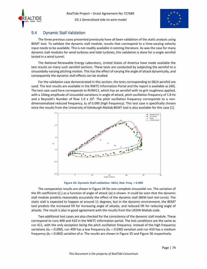
RealTide Project – Grant Agreement No 727689
D3.1 Generalised tide-to-wire model
Page | 74
This Document is the property of RealTide Consortium
9.49.49.49.4 Dynamic Stall ValidationDynamic Stall ValidationDynamic Stall ValidationDynamic Stall Validation
The three previous cases presented previously have all been validation of the static analysis using
BEMT tool. To validate the dynamic stall module, results that correspond to a time-varying velocity
input needs to be available. This is not readily available in existing literature. As was the case for many
dynamic stall modules for wind turbines and tidal turbines, this validation is done for a single aerofoil
tested in a wind tunnel.
The National Renewable Energy Laboratory, United States of America have made available the
test results on many such aerofoil sections. These tests are conducted by subjecting the aerofoil to a
sinusoidally-varying pitching motion. This has the effect of varying the angle of attack dynamically, and
consequently the dynamic stall effects can be studied.
For the validation case demonstrated in this section, the tests corresponding to S814 aerofoil are
used. The test results are available in the NWTC Information Portal and the report is available as [40].
The test case used here corresponds to RUN411, which has an aerofoil with no grit roughness applied,
with a 10deg amplitude of sinusoidal variations in angle of attack, pitch oscillation frequency of 1.8 Hz
and a Reynold’s Number of flow 1.0 x 10⁶. The pitch oscillation frequency corresponds to a non-
dimensionalized reduced frequency, kR of 0.090 (high frequency). This test case is specifically chosen
since the results from the University of Edinburgh Matlab BEMT tool is also available for this case [1].
Figure 34: Dynamic Stall validation -S814, Red. Freq. = 0.090
The comparative results are shown in Figure 34 for one complete sinusoidal run. The variation of
the lift coefficient (CL) as a function of angle of attack (α) is shown. It could be seen that the dynamic
stall module predicts reasonably accurately the effect of the dynamic stall (BEM tool red curve). The
static stall is expected to happen at around 11 degrees, but in the dynamic environment, the BEMT
tool predicts the increased lift for increasing angle of attacks, and reduced lift for reducing angle of
attacks. The result is also in good agreement with the results from the UEDIN Matlab code.
Two additional test cases are also checked for the consistency of the dynamic stall module. These
correspond to runs 409 and 410 in the NWTC information portal. The test conditions are the same as
run 411, with the only exception being the pitch oscillation frequency. Instead of the high frequency
variations (kR = 0.090), run 409 has a low frequency (kR = 0.030) variation and run 410 has a medium
frequency (kR = 0.060) variation of α. The results are shown in Figure 35 and Figure 36 respectively.

RealTide Project – Grant Agreement No 727689
D3.1 Generalised tide-to-wire model
Page | 75
This Document is the property of RealTide Consortium
Figure 35: S814 validation - low frequency Figure 36: S814 validation - medium frequency
Although the correlation is not as good as the earlier case, it can be said that the dynamic stall
behaviour is reasonably represented by the dynamic stall module. One reason for the slight
discrepancy could be some of the default parameters in the dynamic stall module. For these two cases,
the same parameters as the high frequency case was used, as all these parameters were not readily
available. This might have some impact on the final results. Ultimately, the aim is to check the validity
of the dynamic stall computations are performing in an expected manner; and the results seem to
suggest its credibility.
However, it should also be remarked that for the validation cases considered above, the variation of
angle of attack is sinusoidal and hence predictable. In many real-world scenarios, such variations are
arbitrary and hence the validity of such an empirical model in such situations cannot be assured. To
ascertain the validity in such cases, the dynamic stall model should be applied to real world flows, with
experimental measurements.

RealTide Project – Grant Agreement No 727689
D3.1 Generalised tide-to-wire model
Page | 76
This Document is the property of RealTide Consortium
10101010 ELECTRICAL MODELLINGELECTRICAL MODELLINGELECTRICAL MODELLINGELECTRICAL MODELLING AND CONTROL OF GRID AND CONTROL OF GRID AND CONTROL OF GRID AND CONTROL OF GRID
CONNECTED TIDAL CURRCONNECTED TIDAL CURRCONNECTED TIDAL CURRCONNECTED TIDAL CURRENT CONVERSIONS SYSTENT CONVERSIONS SYSTENT CONVERSIONS SYSTENT CONVERSIONS SYSTEMSEMSEMSEMS
The aim of this Chapter is to describe and present in detail the electrical modelling and control of
dynamic grid-connected tidal current conversion systems (TCCSs). The dynamic electrical system
model described in this chapter is to be designed and released as a generic tool for the facilitation and
development of tidal current systems. The first step in order to implement this is to describe the
available literature regarding the modelling of resource-to-grid of tidal current systems. Afterwards,
the various electrical components and the associated control architectures will be presented in detail.
The modelling tools chosen for the electrical system modelling will also be justified. The final section
of this Chapter presents some results from the dynamic open-source simulation tool already designed.
10.110.110.110.1 Review of electrical modelling for tidal current conversion systemsReview of electrical modelling for tidal current conversion systemsReview of electrical modelling for tidal current conversion systemsReview of electrical modelling for tidal current conversion systems
The literature regarding electrical modelling and control of TCCS is limited especially if it is compared
to research in offshore and onshore wind energy systems. An overview of the electrical design in TCCS
and wave energy systems is presented in [42]. Authors present an overview of the electrical design
options for ocean energy converters in general and in addition show the use of power electronics for
generator control and grid connection. They include useful information about the modelling aspects
of electrical generators, generator control, grid-side converter control and variable speed operation
for maximum power point tracking (MPPT). Furthermore, authors in [42] discuss array layouts and
cabling as well as the use of energy storage for ocean energy systems. They dedicate one chapter in
resource-to-wire modelling for tidal turbines and a number of chapters for the grid integration of such
systems. Though [42] is a book that is essential reading for electrical design engineers, researchers and
students in offshore renewables it does not show the simulation models in detail. What is more, the
resource-to-grid modelling presented is based on mathematical formulations and ideal operation of
the control loops compared to the modelling of the physical components.
A comprehensive way of modelling dynamic resource-to-grid TCCSs is presented in a PhD thesis from
the University of Edinburgh [43]. The research shown in [43] aims to present, compare and improve
the options of power transmission for tidal current arrays. The author of the thesis develops dynamic
electromechanical models of tidal current devices in detail, from resource to the grid connection, using
mathematical linear and non-linear programming in MATLAB/Simulink. The tidal models developed
are presented in one chapter and include the tidal resource, the tidal turbine with pitch control, geared
induction and synchronous generators, the power electronics with the generator controller, the grid
side controller, the cables for power transmission, the filters and the grid connection. A key focus
aspect of the study is the power transmission option with onshore converters which is presented in
detail. Using this concept it is possible to generate electricity from tidal current devices but at the same
time keep the highest possible system reliability despite the continuous underwater operation. The
results of the PhD thesis in [43] are compared against data provided by Andritz Hydro Hammerfest.
The study also expands to modelling a number of electrical architectures for tidal current arrays. The
TCCSs developed in [43] are shown in Figure 37 as generalised block diagrams and in Figure 38 with
the associated control loops. More details can be found at the permanent link
http://hdl.handle.net/1842/31089.

RealTide Project – Grant Agreement No 727689
D3.1 Generalised tide-to-wire model
Page | 77
This Document is the property of RealTide Consortium
Figure 37: Block diagrams of single TCCS. a. SCIG and PMSG options with long distance controls. b. SCIG and
PMSG options with back-to-back converters in the nacelle [43].
Figure 38: Block diagram of the single TCCS with long distance controls and the associated control blocks [43].

RealTide Project – Grant Agreement No 727689
D3.1 Generalised tide-to-wire model
Page | 78
This Document is the property of RealTide Consortium
Apart from the two comprehensive studies presented above a number of other research papers
present system level and control modelling, generator comparison modelling and electrical
architecture options for tidal current systems. A brief description of these studies will be presented in
the Sections 10.1.1 to 10.1.3.
10.1.110.1.110.1.110.1.1 Control and system level modelling in tidal current systemControl and system level modelling in tidal current systemControl and system level modelling in tidal current systemControl and system level modelling in tidal current system
Electrical generators used in TCCS are of the same type as those used in wind energy industry. Different
types of generators are controlled using different types of controllers. The controllers’ aim is to make
the generator extract as much as possible energy from the tidal currents by achieving higher power
coefficient. An overview of marine energy systems, including tidal current systems, has been given in
[44]. The focus of the research is on monitoring by collecting data during operation and on the control
of the system in order to achieve maximum power extraction from the marine resource. Even though
the research is not specifically focused on TCCSs, the outputs of the research can be applied to such
systems.
10.1.1.1 Power limitation control system
An important part of the control system in a tidal current turbine is the power limitation mechanism
that operates when the power output is higher than the rated power of the turbine. A comparison
between pitch and stall regulated tidal current turbines is performed in [4]. The research carried out
in [45] was based on horizontal-axis turbines during variable speed operation. The pitch regulated
turbines have variable pitch blades that can feather if the speed of the turbine is above rated speed.
On the other hand, stall regulated turbines have fixed pitch blades and use the inherent blade design
to limit the speed of the turbine at rated levels. Even though in the research both types of speed
regulation have satisfactory results when assessed based on their aim, the stall regulated turbines
generate a lot higher loads on the blades and require more complicated control system design. In [5]
the blades of a horizontal-axis tidal current turbine are designed to achieve feathering by over-
speeding, optimise efficiency and take into account phenomena such as the cavitation. In addition,
authors in [46] describe the potential disadvantages in using the over-speeding method in tidal current
turbines:
• Operating at high rotational speeds increases the voltage generated by the machine.
• Cavitation effect has to be considered.
• Depending on the design, operating at increased rotational speed can increase thrust forces
on the turbine.
• Increased centrifugal forces that can cause blade failure.
Based on the literature reviewed it can be concluded that stall regulated turbines in TCCS have a
number of disadvantages compared to pitch regulated turbines. These include unstable dynamics,
increased out-of-plane bending moments, increased thrust forces and reduced energy yield assuming
both systems have 100% availability.
10.1.1.2 Induction Generators in tidal current systems
The majority of research papers regarding control design in tidal current turbines deal with the use of
novel control strategies in generators. Research that uses SCIG in tidal current turbines is presented in
[47], [48]. Researchers in [49] use long sub-sea cables between the SCIG (Squirrel Cage Induction
Generators) and the voltage-source converter (VSC) in order to transmit power to the grid. In order to
achieve this they use a direct torque controller (DTC) with space vector modulation (SVM) and design
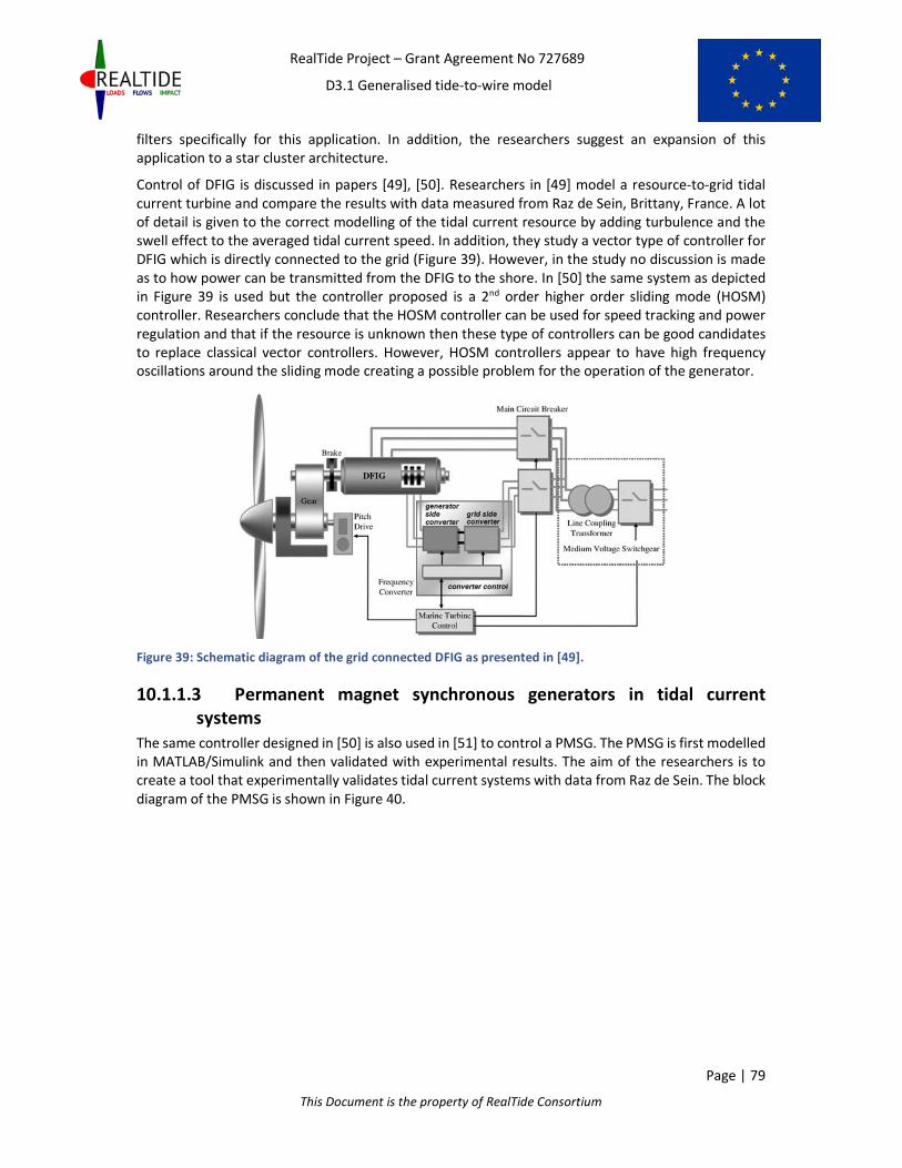
RealTide Project – Grant Agreement No 727689
D3.1 Generalised tide-to-wire model
Page | 79
This Document is the property of RealTide Consortium
filters specifically for this application. In addition, the researchers suggest an expansion of this
application to a star cluster architecture.
Control of DFIG is discussed in papers [49], [50]. Researchers in [49] model a resource-to-grid tidal
current turbine and compare the results with data measured from Raz de Sein, Brittany, France. A lot
of detail is given to the correct modelling of the tidal current resource by adding turbulence and the
swell effect to the averaged tidal current speed. In addition, they study a vector type of controller for
DFIG which is directly connected to the grid (Figure 39). However, in the study no discussion is made
as to how power can be transmitted from the DFIG to the shore. In [50] the same system as depicted
in Figure 39 is used but the controller proposed is a 2nd order higher order sliding mode (HOSM)
controller. Researchers conclude that the HOSM controller can be used for speed tracking and power
regulation and that if the resource is unknown then these type of controllers can be good candidates
to replace classical vector controllers. However, HOSM controllers appear to have high frequency
oscillations around the sliding mode creating a possible problem for the operation of the generator.
Figure 39: Schematic diagram of the grid connected DFIG as presented in [49].
10.1.1.3 Permanent magnet synchronous generators in tidal current
systems
The same controller designed in [50] is also used in [51] to control a PMSG. The PMSG is first modelled
in MATLAB/Simulink and then validated with experimental results. The aim of the researchers is to
create a tool that experimentally validates tidal current systems with data from Raz de Sein. The block
diagram of the PMSG is shown in Figure 40.

RealTide Project – Grant Agreement No 727689
D3.1 Generalised tide-to-wire model
Page | 80
This Document is the property of RealTide Consortium
Figure 40: Schematic diagram of the PMSG tidal current system [51].
Other variations in controlling a PMSG are presented in [52] using passive rectifiers and in [53] using a
fixed pitch blade tidal current turbine. Researchers in [54] perform dynamic stability analysis to a grid
connected tidal current turbine with PMSG. In [52] authors suggest that more than one PMSG can be
connected on the same shaft and use passive rectifiers to connect to the DC link. The extraction of
maximum power from the tidal currents is achieved by knowing the exact tidal currents experienced
by the system and designing the generators accordingly. This system is proposed to have similar
efficiency as a conventional one but less complicated system with lower power converter losses.
However, the main disadvantage of this design is the previous knowledge of the resource that is
required which is not always possible to acquire and may not be accurate.
10.1.210.1.210.1.210.1.2 Generator comparison studies for tidal current systemsGenerator comparison studies for tidal current systemsGenerator comparison studies for tidal current systemsGenerator comparison studies for tidal current systems
Comparing the types of generators in tidal current applications is performed in two separate studies
under different conditions [55], [56]. In [55] authors compare all the types of generators that can be
used in a tidal current system and summarise the advantages and disadvantages of each generator
technology. The summary of their results can be seen in Table 17.
Table 17: Advantages and disadvantages for different generator types. Table adapted from [55].
Type of
Generator Advantages Disadvantages
SCIG
� Full speed range
� No brushes
� Control of reactive and
active power
� Proven technology
� Fully rated BTB power
converters
� Gearbox required
SG
� Full speed range
� Control of reactive and
active power
� Eliminate gearbox (DD
concept only)
� Fully rated BTB power
converters
� Additional converter for field
� Large and heavy generator
(DD concept only)
PMSG
� Full speed range
� Control of reactive and
active power
� Eliminate gearbox (DD
concept only)
� Fully rated BTB power
converters
� Large and heavy generator
(DD concept only)
� Permanent magnets needed

RealTide Project – Grant Agreement No 727689
D3.1 Generalised tide-to-wire model
Page | 81
This Document is the property of RealTide Consortium
� Brushless (low maintenance)
� No power converter for field
compared to SG
DFIG
� Limited speed range ±30%
around synchronous speed
� Control of reactive and
active power
� Reduced rating for power
converters
� Requires slip rings (high
maintenance)
� Gearbox required
The authors concluded that the Direct Drive (DD) PMSG is the most advantageous design due to the
low maintenance and higher efficiency over a wider range of speeds. Due to these capabilities of the
PMSG, the energy generated from a system with DD PMSG is higher compared to the other designs
which also leads to higher revenues. However, DD PMSG are still not a proven technology compared
to the SCIG and the cost to install such generators is higher. In addition, authors explored the possibility
of using DFIG generators due to their popularity with wind energy systems and the lower capital cost
of the overall system because of the lower rated power converters (usually 25% of the full rating).
However, the disadvantages of DFIG, which are mainly the high maintenance requirements, makes the
use of such a generator in an inaccessible underwater system a less attractive option. The discussion
of the authors and the results presented in [55] are comprehensive but there is no reference in the
research paper about the effect of the generator type in the power transmission system of the TCCS.
In [56] researchers compare SCIG and PMSG in a TCCS with direct connection to shore using onshore
power converters. Authors create a dynamic model of a TCCS in MATLAB/Simulink and set three
criteria to compare the two designs.
• First, they look at cost and maintenance of each system.
• Then they study the generator efficiency at different operating speeds and finally,
• Transmission power losses are compared in order to work out the total system
efficiency and total energy generation for each design.
Regarding the cost and maintenance the PMSG generator used in this study is using the same gearbox
as the SCIG, Figure 41, and therefore the cost of the PMSG is not significantly higher than the SCIG. In
terms of generator efficiency, both designs seem to have high efficiencies near the rated power.
However, the PMSG achieved higher efficiencies compared to the SCIG when the TCCS was operating
at below rated power. Regarding power transmission losses the TCCS with the PMSG had 0.35% less
losses compared to the TCCS with the SCIG. Due to the lower losses, the PMSG system can export an
additional 116MWh per year to the grid compared to the SCIG system.

RealTide Project – Grant Agreement No 727689
D3.1 Generalised tide-to-wire model
Page | 82
This Document is the property of RealTide Consortium
Figure 41: Tide-to-grid model developed in MATLAB/Simulink used for generator comparison [55].
10.1.310.1.310.1.310.1.3 Electrical Architecture studies for tidal current systemsElectrical Architecture studies for tidal current systemsElectrical Architecture studies for tidal current systemsElectrical Architecture studies for tidal current systems
Researchers from ABB presented in [57] a comparative study of different power collection options
which were categorised based on the output from the nacelle to: variable frequency AC output (Figure
42a), fixed frequency AC output (Figure 42b) and DC output (Figure 43). All the power collection
options as presented in [57] were compared based on their cost for individual components, cost of
installation and the cost for operation and maintenance for three different installed capacities of tidal
current arrays, 30MW, 100MW and 200MW. Authors concluded that the collection topology with the
least cost is DC-0 and collection topologies VF-0, VF-4, FF-2, DC-1 and DC-3 have comparable losses
with DC-0. However, even though the above mentioned collection topologies have low cost when
considered on their own, the costs change when studied in a 30MW tidal current array. For a tidal
current array, collection topologies with low capital costs are preferred and therefore DC-1 and VF-4
are chosen as preferred options.
Figure 42: (a) Variable frequency from the nacelle collection arrangements. (b) Fixed frequency from the
nacelle arrangements [57].

RealTide Project – Grant Agreement No 727689
D3.1 Generalised tide-to-wire model
Page | 83
This Document is the property of RealTide Consortium
Figure 43: (a) DC output from the nacelle arrangements. (b) Preferred power collection solutions for tidal
current arrays [57].
Another research paper [58] focused on the optimisation of power transmission options for offshore
marine energy systems based on cost of energy and the reactive power compensation. The paper
states that in AC systems the capacitance of the sub-sea cables causes an amount of reactive current
to flow, which limits the capacity for real power transmission. In order to mitigate the reactive current
flowing in the cables reactive power compensation both onshore and offshore is required. Authors in
[58] optimise the reactive power required so that maximum power transmission is achieved and at the
same time meeting the UK Grid Code requirements.
Research studies on power transmission in either AC or DC for tidal current systems are limited and no
conclusion of a preferred solution can be derived. In [43] the research study concluded that when tidal
current devices are clustered per four turbines on offshore platforms it is efficient to use as many
clusters as possible connected to a single cable whose both ends are connected to the grid. Locating
the power converters in the nacelle yields fewer electrical losses compared to locating the power
converters on the offshore platform. However, the difference is minimised because the distance
between the tidal current device and the offshore platform is the least possible. Having the power
converters on an offshore platform is beneficial in terms of accessibility for maintenance and operation
because they are not underwater.
10.210.210.210.2 Methodology for electrical and control modelling for tidal current Methodology for electrical and control modelling for tidal current Methodology for electrical and control modelling for tidal current Methodology for electrical and control modelling for tidal current
conversion systemsconversion systemsconversion systemsconversion systems
The tide-to-grid TCCS developed is depicted in Figure 44.

RealTide Project – Grant Agreement No 727689
D3.1 Generalised tide-to-wire model
Page | 84
This Document is the property of RealTide Consortium
Figure 44: Block diagram of the resource-to-grid model developed.
The Realistic Velocimetry and the tidal turbine options in python code are not part of the dynamic
electrical modelling and are developed separately. The coupling between the turbine model developed
in Python Code and the electrical model is described in Section 11. The dynamic electrical model
accepts a mechanical torque input from the tidal turbine which is fed at the generator rotor. The
components of the electrical modelling include the following:
• The permanent magnet synchronous generator,
• The generator side converter with the associated controller (ZDC),
• The MPPT algorithms and the speed controller,
• The DC link,
• The grid side converter and the associated controller (VOC),
• Grid side power harmonic filters for grid compliance and
• The power transmission for grid connection.
All the parts listed above are described in Sections 10.2.1 to 10.2.7.
10.2.110.2.110.2.110.2.1 The electrical generatorThe electrical generatorThe electrical generatorThe electrical generator
The generator model converts the mechanical torque input from the tidal turbine model to electrical
power. Two widely used generator technologies have been considered, the SCIG and PMSG. Both of
these generator technologies have been implemented in Simulink by the University of Edinburgh. For
the resource-to-grid TCCS open-source tool the PMSG option has been developed with the SCIG option
to be considered for future implementation. Permanent magnet synchronous generators have higher
efficiencies over a wider range of operating speeds compared to SCIGs. This advantage makes them an
attractive option for tidal current developers due to the variability of the tidal current, two high tides
and two low tides within 24 hours and 50 minutes in a semidiurnal tide. A secondary advantage of the
PMSG is the higher power densities due to the use of permanent magnets on the rotor.
The dynamic response of the PMSG model in the dq-axis reference frame is given in (Eq.1) and (Eq.2)
[59].
ÀØÁØ ���Ù�� � ÚÛ� ��Ü�Ù � �Ù��Ù G ÛÝ�Þß�ÝÙ���ÝÙ�� � ÚÛÝ ��ÜÝÙ � �Ù�ÝÙ � Û��Þß��Ù G �Þßà�� (Eq.1)

RealTide Project – Grant Agreement No 727689
D3.1 Generalised tide-to-wire model
Page | 85
This Document is the property of RealTide Consortium
áâ � ã�ä Dà��ÝÙ G �Û� � ÛÝ���Ù�ÝÙO (Eq.2)
The motion equations of the PMSG are given in (Eq.3) [59].
ÀÁ �å��� � Þß
� �Þß�� � Úæ �áâ � �Þß � áß� (Eq.3)
In [59] a detailed description of the quantities involved in (Eq.1) to (Eq.3) is given.
Table 18: Description of quantities of the dynamic PMSG model.
Symbol Description Units Ã�>, Ãç> dq-axis stator currents A è�>, èç> dq-axis stator voltages V c�, cç dq-axis inductances H e> Stator winding resistance Ω B5 Flux amplitude induced by rotor magnets Wb
θr Rotor angular position rad é Moment of inertia of the rotor kgm2 ê Number of pole pairs - �z Mechanical torque from the generator shaft Nm �� Electromagnetic torque Nm Vz Rotor mechanical speed rad/s 6 Rotor and load viscous friction coefficient N
The PMSG chosen model has round rotor and sinusoidal back electromotive force (EMF) has been
chosen. The PMSG may be direct drive or geared depending on the operating speed of the tidal turbine
and the synchronous speed of the rotor. The PMSG model is controlled from the generator side VSC.
The control method used is based on the zero d-axis current control (ZDC) method and is presented in
the following section.
10.2.210.2.210.2.210.2.2 Generator side controllerGenerator side controllerGenerator side controllerGenerator side controller
The generator controller is described in [56] and is based on zero d-axis current control with space
vector modulation (ZDC SVM). The ZDC SVM control method for non-salient pole PMSG is based on
the linear relationship between the stator current magnitude, is, and the electromagnetic torque, Te
when the d-axis stator current of the generator is kept zero and the flux, φr, is kept constant. The block
diagram of the ZDC SVM controller can be seen in Figure 45.
Figure 45: Block diagram of the ZDC SVM generator controller [56].

RealTide Project – Grant Agreement No 727689
D3.1 Generalised tide-to-wire model
Page | 86
This Document is the property of RealTide Consortium
10.2.310.2.310.2.310.2.3 Maximum Power Point TrackingMaximum Power Point TrackingMaximum Power Point TrackingMaximum Power Point Tracking
Maximum power point tracking (MPPT) has one major aim: to control the tidal turbine’s Tip Speed
Ratio λ in order to achieve the highest possible hydrodynamic coefficient Cp. MPPT is responsible for
the efficient operation of the tidal current system at tidal current speeds below rated power. In order
to achieve the efficient operation, first the operating points where maximum Cp is achieved must be
identified. These operating point form the maximum power point curve. After creating the maximum
power point curve the speed and torque of the generator have to be controlled in order to achieve
these optimised operating points. This is achieved by the speed controller.
The maximum power point curve (MPPC) identifies all the operating points with maximum Cp. The
maximum power point curve modelled in this paper is based on equation (Eq.4) where k is a constant.
�z�3ë�@ � ì ∙ Vy�vë�@� ⇔ Vy�vë�@ � ²�z�3ë�@ì (Eq.4)
An example of a MPPC acquired by simulating the University of Edinburgh’s XMED turbine is shown in
Figure 46.
Figure 46: Torque speed curves for different tidal current velocities for a simulation model of XMED turbine.
The peak mechanical torque is identified (blue dots) and a curve is fitted based on Eq.4 which forms the MPPC.
The speed controller is responsible of comparing the optimum generator speed, ωoptGen, acquired by
equation (Eq.4) and actual generator speed, ωmecGen, which is measured, in order to produce a
reference signal for the electromagnetic torque of the generator. The reference signal of the
electromagnetic torque, Te*, is used as input to the generator controller ZDC SVM shown in Figure 45.
The block diagram of the speed controller is shown in Figure 47. More details can be found in [42],
[43].

RealTide Project – Grant Agreement No 727689
D3.1 Generalised tide-to-wire model
Page | 87
This Document is the property of RealTide Consortium
Figure 47: Speed controller block diagram as modelled for the resource-to-grid TCCS tool.
10.2.410.2.410.2.410.2.4 The DC linkThe DC linkThe DC linkThe DC link
All the power from the generator that is converted by the generator side VSC passes through the DC
link. The DC link voltage is kept constant by converting the input power to the DC link into a constant
voltage and frequency on the grid side. This conversion is achieved by the grid side VSC which is
controlled by the grid side controller discussed in Section 10.2.5. The DC link model is composed of an
ideal capacitor, a discharging resistance and an equivalent series resistance (ESR). The diagram of the
DC link model is presented in Figure 48.
Figure 48: Block diagram of the DC link model implemented in Simulink and OpenModelica.
10.2.510.2.510.2.510.2.5 Grid side controllerGrid side controllerGrid side controllerGrid side controller
The power generated by the TCCS is delivered to the grid through a VSC. The inverter is controlled by
a PWM scheme called voltage oriented control (VOC) with decoupled controllers which ensures a
constant DC link voltage, constant frequency output of 50Hz on the AC side and control over the
amount of reactive power flowing based on grid requirements. The VOC scheme is based on (Eq.5) and
is shown in Figure 49:
ïð����� � � ñòóô ���õ∗ � ��õ� G òôô ����õ∗ � ��õ���ö G ÞõÛõ�Ýõ G ð�õðÝ���� � � ñòóô ��Ýõ∗ � �Ýõ� G òôô ���Ýõ∗ � �Ýõ���ö � ÞõÛõ��õ G ðÝõ (Eq.5)

RealTide Project – Grant Agreement No 727689
D3.1 Generalised tide-to-wire model
Page | 88
This Document is the property of RealTide Consortium
Figure 49: VOC controller as implemented in the resource-to-grid TCCS.
10.2.610.2.610.2.610.2.6 Grid side power harmonic filtersGrid side power harmonic filtersGrid side power harmonic filtersGrid side power harmonic filters
In order to make the TCCS grid compliant power harmonic filters are installed at the output of the grid
side converter. The power filters include a line reactor to reduce line current distortion and low-pass
or single-tuned power harmonic filters to reduce harmonic distortion due to the PWM and the non-
linear electrical components.
10.2.710.2.710.2.710.2.7 Power transmissionPower transmissionPower transmissionPower transmission
The power transmission includes a transformer to step-up the low voltage output of the VSC
to kV range and three-phase power cables for onshore connection to the grid. Increasing the voltage
with a transformer is essential in order to ensure minimum losses in the power cables. The cable type
and the exact voltage depends on the distance between the VSC and the grid as well as the type of
connection implemented based on the variations described in [43], [57].
10.2.810.2.810.2.810.2.8 Modelling tools for grid connected tidal current systemsModelling tools for grid connected tidal current systemsModelling tools for grid connected tidal current systemsModelling tools for grid connected tidal current systems
a) Tidal Bladed:
Tidal bladed is a commercial industry-related tool for simulating tidal turbines and combines
all the components for tidal current turbine design in a single software package. The main focus of
Tidal Bladed is tidal turbine rotor and structural design. Electrical and control components are also
included but power output is estimated with electrical loss models and grid side modelling limited.
b) MATLAB/Simulink:

RealTide Project – Grant Agreement No 727689
D3.1 Generalised tide-to-wire model
Page | 89
This Document is the property of RealTide Consortium
MATLAB is a commercial multi-paradigm numerical computing environment and fourth-
generation programming language. A proprietary programming language developed by MathWorks,
MATLAB allows matrix manipulations, plotting of functions and data, implementation of algorithms,
creation of user interfaces, and interfacing with programs written in other languages, including C and
C++ [60]. Simulink is also developed by MathWorks and is a graphical programming environment for
modelling, simulating and analysing multidomain dynamic systems. It offers tight integration with the
rest of the MATLAB environment. Simulink is one of the most common commercial software used for
tide-to-grid electrical and control modelling because it offers:
• Dynamic simulation capabilities of electrical components.
• The ability to easily work on the frequency domain after the time domain simulation.
Frequency domain results are crucial in understanding cable and transformer-cable
interaction and resonance.
• The ability to parameterise the models using MATLAB variables and expressions. This
feature is important in order to optimise models in an analytic way and scale models
according to needs.
• Control design capabilities and the available control and electrical components.
• Fast simulation mode for discretised models.
c) OpenModelica/JModelica
OpenModelica is an open-source Modelica-based modelling and simulation software which is
used by both industry and academia. OpenModelica has a graphical user interface that provides the
user an easy way to model, edit models and simulate models as well as plot the results. In addition,
OpenModelica utilises the Modelica Standard Library which offers ready to use electrical, control and
mechanical components suitable for the development of a resource-to-grid TCCS. JModelica [61] on
the other hand, shares similar features as OpenModelica but its operation is controlled primarily by
Python code and is focused on the optimisation of Modelica models. Both software packages,
OpenModelica and JModelica, support the Functional Mock-up Interface (FMI) [62] which is a standard
for coupling and information exchange between dynamic models. It provides an interface for coupling
different simulation tools in a single environment. The FMI is supported by several software such as
Dymola, ANSYS and SIMPACK.
OpenModelica and JModelica offer a number of advantages for the tide-to-grid electrical TCCS model
which is developed. Firstly, the FMI can be fully controlled using python code which makes the coupling
of the BEMT tidal turbine model developed in python straightforward. In addition, it offers ready to
use electrical components and control structures as well as support for problem solving. What is more,
OpenModelica and JModelica can be controlled from a python script making it easy to implement
custom made control algorithms and optimisation techniques to improve the performance of the TCCS.
Finally, both software are open-source and are supported with new versions every year.
10.310.310.310.3 Condition Monitoring Based on Model Based EstimationCondition Monitoring Based on Model Based EstimationCondition Monitoring Based on Model Based EstimationCondition Monitoring Based on Model Based Estimation
10.3.110.3.110.3.110.3.1 IntroduIntroduIntroduIntroduction to modelction to modelction to modelction to model----based estimationbased estimationbased estimationbased estimation
In a model-based method, the condition of the physical system is represented in a dynamic model. The
goal of this method is to reproduce the condition of the physical system in the model and therefore, if
any mismatch between the data acquisition and the model estimation is found, the system will act

RealTide Project – Grant Agreement No 727689
D3.1 Generalised tide-to-wire model
Page | 90
This Document is the property of RealTide Consortium
accordingly to bring the system into a safe state. In this section we will describe the model-based
monitoring principles and its application in RealTide project. The electrical, physical and dynamic
model developed as part of this deliverable can be used for model-based monitoring which is part of
WP4.
In a first instance, it is necessary to introduce the concepts of analytical redundancy and residual
generation on the assumption of a perfect model. Figure 50 shows a schematic description of a
redundant model based parameter estimation applied on a generic tidal turbine. As can be seen,
different measurements are collected from the tidal turbine sensors and implemented into two
different models. In the model �z represent the actual measurement that has been measured directly
or indirectly from the tidal turbine.
Figure 50: Schematic description of the residual generator
An often applied method to reconstruct �z� is an on-line parallel estimation of input-output
relationship, based in a model which describes a certain physical phenomena which allows to estimate �z analytically. Consider the following nominal model that describes the transfer behavior of the
system or a part of the system under monitoring: ��� � ÷z� �@�
In this scheme, ��� represents the model 1 estimated variable, for which a redundancy will be
established, and �@� the model input vector [�#, �0] which can be either a measured or model
estimated variable. Each model, will estimate the actual measurement (�z by using different physical
principles. In the same way, �z can also be estimated by using a different model: ��� � ÷z� �@�
Where both ��� and ��� are an estimate of �z and is called analytical or software redundancy. ÷z�
and ÷z� represent the transfer function for the models 1 and 2 respectively. The output parameters �g�, �g�, … , �g@, represent the generated residual after comparing different input signals. These

RealTide Project – Grant Agreement No 727689
D3.1 Generalised tide-to-wire model
Page | 91
This Document is the property of RealTide Consortium
residuals can be used later as an estimator in order to check the correct operation of the element
under monitoring. One generic way to calculate a residual could be:
�g@ � ù�? � �úù Where �? and �ú are generic variables referring the same physical magnitude that could be either
estimated (for example ��� or ���) or measured (for example �z).
Even though the principle behind this technique promises a simple on-line implementation and seems
easy to be understood, is not easy or even impossible to implement in some cases due to the difficulty
or even impossibility on generating a precise analytical model if the process is complex. For that
reason, in order to generate an efficient model, it is necessary to choose the variables involved in it
carefully i.e. ones easily measurable and comparable in the real device.
10.3.210.3.210.3.210.3.2 DynamicalDynamicalDynamicalDynamical behaviour modelbehaviour modelbehaviour modelbehaviour model
Figure 51 shows a simplified model that could be used for modelling the dynamical behaviour of the
device in a simplified way which allows, among other things, the evaluation of loads over the different
elements of the device. The model shows the general structure with the functional blocks that the
turbine model should include. Likewise, each block may consist of several different models which be
developed and described in depth in further deliverables within WP3.
Figure 51: Dynamical behaviour model
10.3.2.1 Signal-based fault detection of the power electronics
Variable-speed AC motors usually consist of a AC-DC converter (rectifier) and a three-phase DC-AC
converter (inverter) that generates the three-phase system with variable frequency and amplitude as
shown in Figure 52. In this section we will focus on the most typical failures that may appear and how
can be detected with signal-based methods.

RealTide Project – Grant Agreement No 727689
D3.1 Generalised tide-to-wire model
Page | 92
This Document is the property of RealTide Consortium
Figure 52: Variable speed AC motor diagram.
a) AC-DC converter (rectifier) The most relevant faults in rectifiers are the line disconnection of one phase and faulty diodes.
Significant impacts of the faults are to be observed in the run of the DC-link voltage f�. As represented
in Figure 53, the signal shows significantly higher ripples in the presence of faults:
Figure 53: DC-link voltage �� in the presence of different faults (sampling frequency 2 kHz)
An easy and robust way for rectifier fault detection is the evaluation of the signal’s variance: �́ � � è��ûf�ü
As expected, the variance increases in case of faults from the corresponding values within the healthy
state. As the variance depends on the load current ýhy$� it is computed for normal state in dependence
on the load current as shown in the following figure:
Figure 54: Variance of DC-link voltage �� for different faults
b) DC-AC converter (inverter)

RealTide Project – Grant Agreement No 727689
D3.1 Generalised tide-to-wire model
Page | 93
This Document is the property of RealTide Consortium
Inverter faults and also stator winding faults generate characteristic harmonic of the stator current
vector. The stator current can be described as:
ýþ�b� � 23 �ýþ��b� G ýþ��b�:�?� 4# G ýþ#�b�:�?0 4# �
If the expression above is transformer into an orthonormal ¦ and � component coordinate system: ýþ�b� � ýþ�b� G à ýþ£�b� � ýþS�b�:?����
In the fault-free case the trajectory of the current vector forms a circle, which deforms to an ellipse in
the case of a stator winding fault (Figure 55 a), and to other trajectories for inverter faults and current
sensor faults. Figure 55 b, represents a fault of an inverter IGBT (Insulated Gate Bipolar Transistor),
Figure 55 c the fault due to phase 2 disconnection and Figure 55 d a current sensor fault. In case of
these faults the spectrum of the current vector contains a positive and negative frequency: ýþ�b� � ýþ̅�:?��v,+�� G ýþ̅��:?���v,+¼��
Where Vþ is the stator angular frequency.
Figure 55: Stator current vector trajectories.
In this point, we can also define a set of fault-symptoms and, attending at the sign of the residuals
terms defined bellow Table 19, it will be possible to identify the fault modes of the AC motor.

RealTide Project – Grant Agreement No 727689
D3.1 Generalised tide-to-wire model
Page | 94
This Document is the property of RealTide Consortium
Table 19. Fault symptom table for the PWM converter and stator windings
Residual terms shown in the table have been defined as follow: ����b� � ýþ�� �b� � ýþ�� �b� ��#�b� � ýþ�� �b� � ýþ#� �b� �#��b� � ýþ#� �b� � ýþ�� �b� �́ �� � fþ���b� �́ ��� � fþ��� �þS � |ýþS| � |ýþ��b� G ýþ��b� G ýþ#�b�| 10.410.410.410.4 Results from the tidal current conversion systemResults from the tidal current conversion systemResults from the tidal current conversion systemResults from the tidal current conversion system
In this Section preliminary results from the electrical side of the TCCS developed in OpenModelica will
be shown. Due to the fact that there is no tidal turbine in the electrical system, the mechanical torque
input to the generator shaft will be predefined. The coupled electrical model with a tidal turbine
developed in python will be depicted in Section 3. The TCCS is based on the XMED system of the
University of Edinburgh.
10.4.110.4.110.4.110.4.1 Model response to step change of mechanical torque inputModel response to step change of mechanical torque inputModel response to step change of mechanical torque inputModel response to step change of mechanical torque input
Figure 56 shows preliminary results from the operation of the simulated TCCS with step changes.
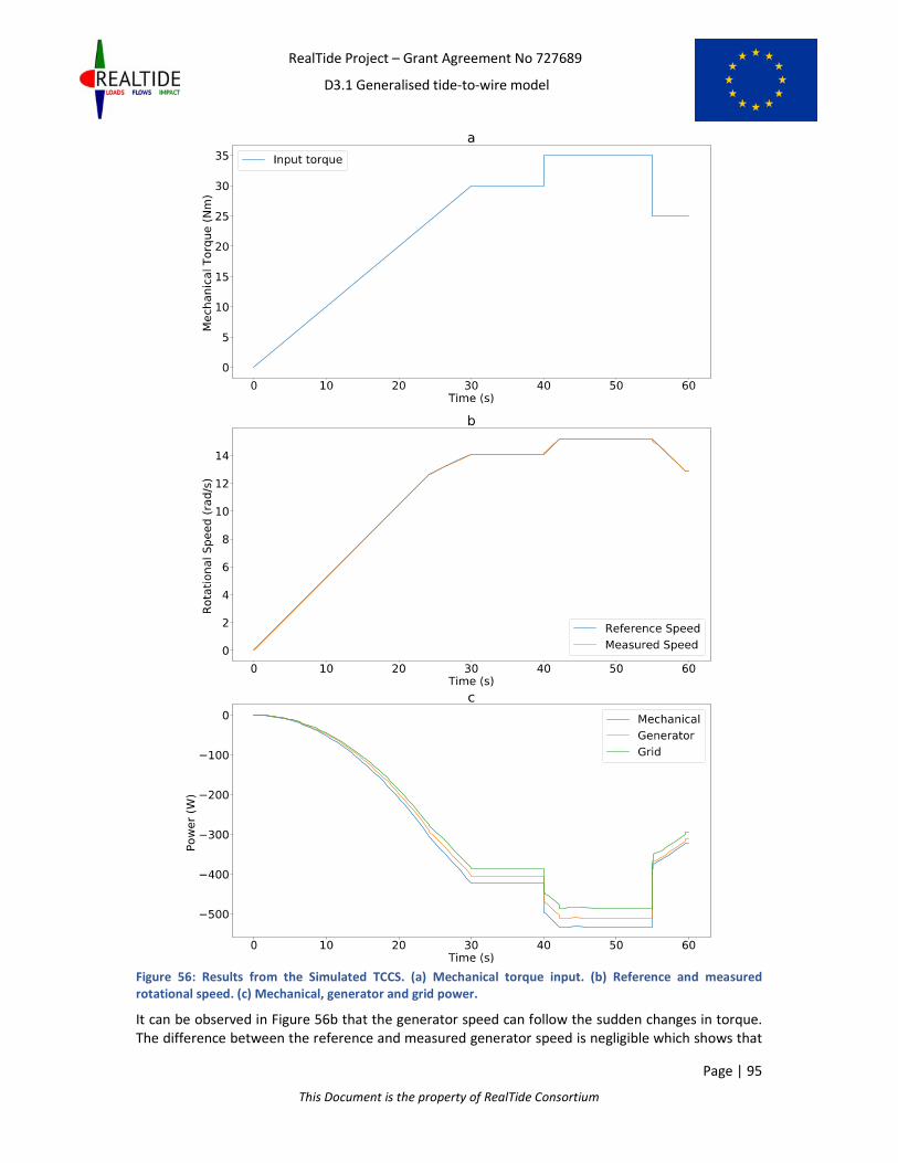
RealTide Project – Grant Agreement No 727689
D3.1 Generalised tide-to-wire model
Page | 95
This Document is the property of RealTide Consortium
Figure 56: Results from the Simulated TCCS. (a) Mechanical torque input. (b) Reference and measured
rotational speed. (c) Mechanical, generator and grid power.
It can be observed in Figure 56b that the generator speed can follow the sudden changes in torque.
The difference between the reference and measured generator speed is negligible which shows that

RealTide Project – Grant Agreement No 727689
D3.1 Generalised tide-to-wire model
Page | 96
This Document is the property of RealTide Consortium
the speed controller is operating optimally. Figure 56c shows the power which is measured at 3 points
in the system. The mechanical power is the input to the generator, the generator power is the 3-phase
electrical power at the generator stator and the grid power is the electrical power after considering
losses in the back-to-back power converters. The filtered voltage and current output of the generator
are shown in Figure 57.
Figure 57: Generator stator voltage and current. (a) Phase A stator current. (b) Phase A stator current zoomed
at 40s simulation time. (c) Phase A stator voltage. (d) Phase A stator voltage zoomed at 40s simulation time.
10.4.210.4.210.4.210.4.2 Model response to variable change of mechanical torque inputModel response to variable change of mechanical torque inputModel response to variable change of mechanical torque inputModel response to variable change of mechanical torque input
Figure 58 shows preliminary results from the operation of the simulated TCCS with variable realistic
type input.
The mechanical torque input to the generator shaft shown in Figure 58a is slowly increasing with
sinusoidal variations with 5 and 10 seconds period. The reference and measured rotational speed of
the generator, shown in Figure 58b, are almost identical. The speed controller manages to generate
the appropriate reference electrical torque signal to the generator side controller in order to achieve
the desired speed. The reference speed is also limited by the maximum acceleration and deceleration
of the generator. Finally, the mechanical power input to the generator, the electrical power output of
the generator and the power exported to the grid are depicted in Figure 58c. It is observed that losses
occur at the different conversion stages but are not significant. For these preliminary results the power
transmission system is not included and for the losses from the electrical power output of the
generator to the grid power exported only the efficiency of the BTB converters is included.

RealTide Project – Grant Agreement No 727689
D3.1 Generalised tide-to-wire model
Page | 97
This Document is the property of RealTide Consortium
Figure 58: Results from the Simulated TCCS with variable input. (a) Mechanical torque input. (b) Reference and
measured rotational speed. (c) Mechanical, generator and grid power.
Figure 59 shows the generator output current and voltage for the simulation presented in Figure 58.

RealTide Project – Grant Agreement No 727689
D3.1 Generalised tide-to-wire model
Page | 98
This Document is the property of RealTide Consortium
Figure 59: Generator stator voltage and current for variable mechanical torque input. (a) Phase A stator
current. (b) Phase A stator current zoomed at 40s simulation time. (c) Phase A stator voltage. (d) Phase A stator
voltage zoomed at 40s simulation time.
The results from the electrical model presented in Section 10.4.1 and 10.4.2 are based on a user
defined mechanical torque input to the generator shaft. In an actual TCCS the mechanical torque input
to the generator shaft comes from the tidal turbine which is affected by the tidal flow speed and the
speed of the generator. Results with a coupled BEMT model developed in python code and the
electrical generator to grid model presented here will be discussed in Section 11.

RealTide Project – Grant Agreement No 727689
D3.1 Generalised tide-to-wire model
Page | 99
This Document is the property of RealTide Consortium
11111111 COUPLED COUPLED COUPLED COUPLED BEMTBEMTBEMTBEMT AND ELECTRICAL MODELAND ELECTRICAL MODELAND ELECTRICAL MODELAND ELECTRICAL MODEL
In this Section the coupling between the BEMT model, developed by BV in python, and the electrical
TCCS model described above will be presented. This coupling using open-source software tools has
never been presented before and can be the basis of a resource-to-grid TCCS tool with great impact in
both tidal industry and research development.
The coupling process involves converting the Modelica model (.mo file) to a Functional Mock-up Unit
(FMU) and managing the electrical model inputs and outputs from python. Managing the FMU from
python requires a python library that can control FMUs such as pyFMI or FMPy. Figure 60 shows to
process to convert the Modelica electrical model to an FMU. The FMU is a .zip file which contains:
• An XML file which defines all the variables in the model and sets initial values.
• All the equations of the model defined as a set of C functions.
• Other data such as tables, documentation and user interface options.
Figure 60: Process to generate the FMU of the electrical model developed in OpenModelica and load it in
python
After generating the FMU file the BEMT python code and the FMU loaded in python need to exchange
information at regular intervals. This is because the turbine operation is affected by the generator
speed and the generator speed is affected by the mechanical torque input to the generator shaft.
Therefore it is of crucial importance that the exchange of information between the BEMT code and the
FMU, which contains the electrical model, is at regular intervals in order to capture the realistic
operation. This is achieved by having both, the BEMT code and the FMU, in a while time loop which
advances at this regular time step. An overview of this process is depicted in Figure 61.
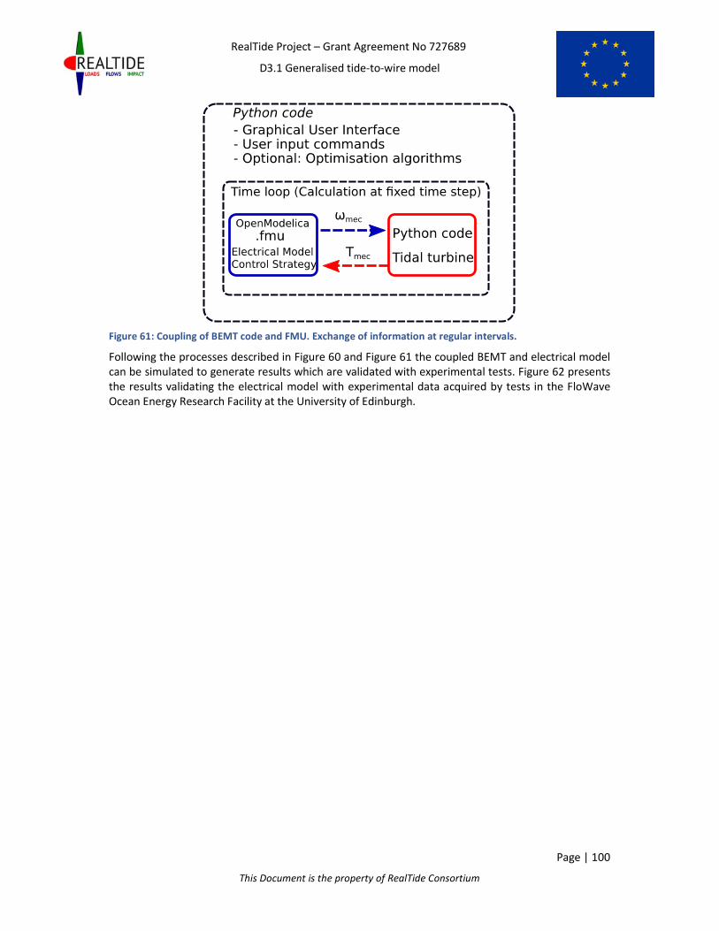
RealTide Project – Grant Agreement No 727689
D3.1 Generalised tide-to-wire model
Page | 100
This Document is the property of RealTide Consortium
Figure 61: Coupling of BEMT code and FMU. Exchange of information at regular intervals.
Following the processes described in Figure 60 and Figure 61 the coupled BEMT and electrical model
can be simulated to generate results which are validated with experimental tests. Figure 62 presents
the results validating the electrical model with experimental data acquired by tests in the FloWave
Ocean Energy Research Facility at the University of Edinburgh.

RealTide Project – Grant Agreement No 727689
D3.1 Generalised tide-to-wire model
Page | 101
This Document is the property of RealTide Consortium
Figure 62: Comparison of experimental and simulated results using a coupled BEMT and electrical model in
python. (a) Tidal current velocity input. (b) Mechanical torque. (c) Turbine rotational speed.
It is observed that the simulated flow used as input to the model closely matches the actually measured
tidal current flow. The same applies for the rotational speed of the turbine which is kept constant. In
this system the reference generator speed is constant and therefore the MPPT system described in
Section 10.2.3 is bypassed and the input to the speed controller is a constant signal. In terms of torque
output from the tidal current turbine it is shown that there is a difference between experimental and
simulated data. The reasons can be explained by the development of the BEMT code in Section 6. The
validation of the model will continue with further modelling and experimental data.
Finally, the coupled electrical model with the BEMT code is simulated with the MPPT system enabled.
The tidal current velocity input to the model comes from the experimentally acquired tidal current
measurements depicted in Figure 62 and the results of this simulation are presented in Figure 63.

RealTide Project – Grant Agreement No 727689
D3.1 Generalised tide-to-wire model
Page | 102
This Document is the property of RealTide Consortium
Figure 63: Results from the operation of the coupled BEMT and electrical model with the MPPT system
enabled. (a) Tidal current velocity from measured experiment. (b) Mechanical torque of the tidal turbine. (c)
Rotational speed of the tidal current turbine. (d) Power at different levels of the resource-to-grid system. (e)
Hydrodynamic coefficient of the turbine. (f) Thrust force on the turbine.
The results above show that the resource-to-grid TCCS can operate at maximum hydrodynamic
coefficient and extract significant amounts of power from the tidal currents. Figure 63c depicts the
reference and the measured rotational speed of the tidal turbine. It is observed that the measured
speed follows the reference closely which makes the tidal current turbine efficient as shown in Figure
63e. The efficiency of the turbine is fluctuating around 0.48. The power of the tidal current input to
the turbine, the mechanical power input to the generator and the electrical power output of the
generator are depicted in Figure 63d. The average electrical power is 4% lower compared to the
average mechanical power. Further research will focus on validating the maximum power point
tracking system experimentally and on the development of a more user friendly resource-to-grid TCCS
tool.

RealTide Project – Grant Agreement No 727689
D3.1 Generalised tide-to-wire model
Page | 103
This Document is the property of RealTide Consortium
12121212 CCCCONCLUSIONONCLUSIONONCLUSIONONCLUSION
The objective of the task T3.1 has been achieved by the development of a time dependant tide-to-wire
model using blade element momentum theory (BEMT) to calculate the torque and thrust on a tidal
turbine. From an input of the tidal conditions, the tool is also able to predict the power output in terms
of electrical parameters and accounts for realistic tidal conditions such as turbulent and unsteady flow.
The program architecture using Python code and equations used are fully detailed in this report and
some improvements of the BEM theory have been implemented in the code and validated by several
application cases based on previous experiments or simulations. The methodology for the electrical is
also fully explained as well as the condition monitoring based on model based.
In T3.3, UEDIN will integrate the tide-to-wire model in an open source Computational Fluid Dynamics
solver. The Figure 64 shows a schematic diagram showing this integration, with its interactions with
the electrical module and a CFD code illustrated.
Figure 64: Coupling of BEMT tool within RealTide project
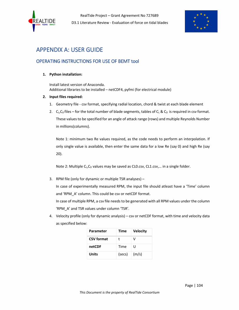
RealTide Project – Grant Agreement No 727689
D3.1 Literature Review - Evaluation of force on tidal blades
Page | 104
This Document is the property of RealTide Consortium
APPENDIX A: USER GUIAPPENDIX A: USER GUIAPPENDIX A: USER GUIAPPENDIX A: USER GUIDEDEDEDE
OPERATINGOPERATINGOPERATINGOPERATING INSTRUCTIONS FOR USE OF INSTRUCTIONS FOR USE OF INSTRUCTIONS FOR USE OF INSTRUCTIONS FOR USE OF BEMT toolBEMT toolBEMT toolBEMT tool
1. Python installation:
Install latest version of Anaconda.
Additional libraries to be installed – netCDF4, pyfmi (for electrical module)
2. Input files required:
1. Geometry file - csv format, specifying radial location, chord & twist at each blade element
2. CL,CD files – for the total number of blade segments, tables of CL & CD is required in csv format.
These values to be specified for an angle of attack range (rows) and multiple Reynolds Number
in millions(columns).
Note 1: minimum two Re values required, as the code needs to perform an interpolation. If
only single value is available, then enter the same data for a low Re (say 0) and high Re (say
20).
Note 2: Multiple CL,CD values may be saved as CL0.csv, CL1.csv,… in a single folder.
3. RPM file (only for dynamic or multiple TSR analyses) –
In case of experimentally measured RPM, the input file should atleast have a ‘Time’ column
and ‘RPM_A’ column. This could be csv or netCDF format.
In case of multiple RPM, a csv file needs to be generated with all RPM values under the column
‘RPM_A’ and TSR values under column ‘TSR’.
4. Velocity profile (only for dynamic analysis) – csv or netCDF format, with time and velocity data
as specified below:
Parameter Time Velocity
CSV format t V
netCDF Time U
Units (secs) (m/s)

RealTide Project – Grant Agreement No 727689
D3.1 Generalised tide-to-wire model
Page | 105
This Document is the property of RealTide Consortium
5. Experimental comparison (only for comparative plots) – Data with experimental comparison
could be read in csv or netCDF format. The names of columns for data are specified in the
tables below:
a. Time comparison:
Parameter Time Thrust Torque Power CT CQ CP
Units (secs) (N) (Nm) (W) (-) (-) (-)
Column name Time R_THRS R_TRQU R_POW CT CQ CP
b. TSR comparison:
Parameter TSR Thrust Torque Power CT CQ CP
Units (-) (N) (Nm) (W) (-) (-) (-)
Column name TSR Thrust Torque Power CT CQ CP
c. Comparison for distribution along blade length:
Parameter Length Along Blade Data for Blade ‘N
(N starts from 0)
Units (m) Shear Force in (N)
Bending Mt. in (Nm)
Column name r BladeN
3. Opening Python:
Copy all the python scripts into a single folder. Open Anaconda Navigator and Launch Spyder.
Open all the 5 python scripts (Refer Sl. 3).
4. Python scripts:
1. main.py – This script calls all the other scripts within itself. You only need to run this one.
2. UserInterface.py – Includes all the codes related to the input GUI.
3. algorithms.py – Includes all the algorithms for BEMT computations such as Ning’s single
variable parametrization, iterative algorithm, high induction correction methods, tip & hub
loss functions.
4. DynamicStall.py – Includes the entire dynamic stall module with all its sub-functions
5. postprocess.py – Includes the commands required for launching of the postprocessor GUI.
5. Default Folder specification (only required for first use):

RealTide Project – Grant Agreement No 727689
D3.1 Generalised tide-to-wire model
Page | 106
This Document is the property of RealTide Consortium
Before executing the code, a default path variable needs to be set on UserInterface.py
at line 116 (inside class cls_inp). Although the program can read values from the user, some
variables need to be initialized, and this is done using the path variable. This should point
towards a folder which contains some csv files pertaining to geometry of blades (geom.csv),
and CL,CD data (CL0.csv,CD0.csv). These can be changed later on in the GUI. After making the
changes, save the file UserInterface.py.
6. Executing the code:
To execute the code, open main.py and press ‘Run File’ (F5). If the code throws an error that
‘Pyimage does not exist’, then you need to restart the kernel at the Python console (Ctrl + .)
7. Input UI – Entering Blade Geometry:
Click the button ‘Input Blade Geometry’ under section ‘1.Blade Data’. In the new
window which opens, all the major geometrical parameters of the blade and the
environmental parameters can be entered.
To load the geometry csv file, click ‘Load Geometry Data’ and specify the csv file. The
table updates automatically, but it still shows traces of old data. To view the data that is
loaded, click the ‘OK’ button, which closes the window. If the same window is reopened again,
then the geometry data, can be seen as updated.
8. Input UI – Entering Lift and Drag Data:
1. Enter the number of blade segments [m]. For more info about this, the info button may be
used. Then, click the button ‘Input Lift and Drag Coefficients’ under section ‘1.Blade Data’.
This opens a new window with the default values of CL, and CD loaded. The number of
vertical segments in the window would refer to the number of blade segments entered
earlier.
2. For each m, the lift and drag coefficients can be entered by clicking the corresponding
buttons on the top of the vertical segment. Alternatively, if all the CL, CD data is stored in a
single folder with the naming convention as specified in Sl. 2.2, this folder could be specified
by clicking the ‘Read CL,CD from folder’ button at the bottom of the window.

RealTide Project – Grant Agreement No 727689
D3.1 Generalised tide-to-wire model
Page | 107
This Document is the property of RealTide Consortium
3. The user also needs to enter the start of each segment in the entry boxes provided above
each segment. Note that for the first segment, this is automatically updated as the hub
radius.
4. Once done, click the ‘Confirm’ button at the top.
5. Note: The window is not designed very user-friendly with scroll-bars. So, if the number of
segments is large, the window size would be too large to display.
6. In case the CL, CD provided is not for angle of attacks from -180deg to +180deg, then the
‘Viterna Extrapolation’ button will be activated. However, for this to happen, the data
needs to be stored in the system and this happens only when the window is closed by the
Confirm button. When it is reopened, you can see the user entered values of CL, CD and
option for Viterna extrapolation, if needed.
9. Inflow Velocity – Experimental Data:
1. For experimental measurements, the corresponding radio-button under section ‘2.Inflow
Velocity’ needs to be clicked. This opens up two boxes, where the start and stop time for
analysis may be specified.
2. The user can select options of ‘Variation with depth’ and ‘Variation with time’.
Experimental measurements always have a variation with time; however this is not linked
to the corresponding button. Therefore, this should be checked.
3. Click the ‘Input Velocity Profile’. This opens a file specification window, where the user can
specify the velocity profile prepared as per Sl. 2.4.
4. For variation with depth, the default power law is 1/15.
10. Inflow Velocity – Environmental conditions:
1. Click the ‘Environmental conditions’ radio-button. This opens up entry boxes to specify the
current velocity due to tides, waves and winds. The value of each may be specified, or if
only the total is known, then this can be specified in any of the columns.
2. The user can select options of ‘Variation with depth’ and ‘Variation with time’.
3. If ‘variation with time’ is checked, it opens the input dialog box where the input file needs
to be specified.

RealTide Project – Grant Agreement No 727689
D3.1 Generalised tide-to-wire model
Page | 108
This Document is the property of RealTide Consortium
4. Otherwise, it opens another window which asks for the power law factor. Note that the
velocity value is updated in accordance with the current velocities specified in the previous
window.
11. Inflow Velocity – Steady flow:
1. If only constant velocity cases are to be computed, then the ‘Experimental conditions’
radio-button can be clicked, with ‘Variation with time’ unchecked.
2. This opens a window similar to the one in Sl. 10.4, but has more data inputs required.
3. Enter the steady stream velocity
4. The rest of the data needs to be entered only if there is variation with depth. This data is
used to interpolate the velocity data in the depth direction. Explanation of the parameters
are given in the figure just below.
12. Plot Velocity Profile:
This button is only to give the user a graphical indication of how the program has taken the
depth variation into computation. Note that these computations depend on the correctness
of the data entered for the dimensional parameters in Sl. 11.4.
13. Input RPM Data:
1. Constant RPM – the value needs to be entered in the entry box
2. Varying RPM – only for dynamic analysis. The csv or netCDF file as specified in Sl. 2.3 may
be input. Note that the time stamp for this data need not match with that for the velocity
profile. The program computes at the time steps given in the velocity profile, and
interpolates for RPM values at these time steps.
3. Multiple RPM – only valid for static analysis cases. The csv file as specified in Sl. 2.3 may
be input.
4. Feedback RPM – for further implementation of coupling with electrical module.
14. Select relevant BEMT modules.
15. RUN to execute the program.

RealTide Project – Grant Agreement No 727689
D3.1 Generalised tide-to-wire model
Page | 109
This Document is the property of RealTide Consortium
OPERATINGOPERATINGOPERATINGOPERATING INSTRUCTIONS FOR INSTRUCTIONS FOR INSTRUCTIONS FOR INSTRUCTIONS FOR POSTPROCESSINGPOSTPROCESSINGPOSTPROCESSINGPOSTPROCESSING
When the computations are completed, the post-processing window opens as a GUI.
16. Time plots:
These are typically required for a dynamic analysis, with the input velocity profile having a
variation with time. Click on ‘Time’ under list for x values. The possible plot options are:
a) Forces – Thrust/Torque/Power/CT/CQ/CP
b) Root Bending moment – for each blade
c) Operating Conditions – Inflow velocity & RPM
The relevant TSR can also be selected.
17. TSR plots:
These are typically required when performing a static analysis for multiple RPM inputs. Click
on ‘TSR’ under list for x values. The possible plot options are:
a) Forces – Thrust/Torque/Power/CT/CQ/CP
b) Root Bending moment – for each blade
c) Operating Conditions – Inflow velocity & RPM
18. Force distribution along length of blade:
This data would be required for strength analysis of the blades, or for troubleshooting the
calculations. Click on ‘Length’ under list for x values. The possible plot options are:
a) Shear Force
b) Bending Moment
c) Elemental Forces or Body Forces on the blade (Axial and Tangential)
Within a single graph, the same item can be plotted for multiple blades. The corresponding
TSR can be selected, and the relevant time also can be selected (for dynamic analysis).
19. Comparison with experimental data:
1. The number of experimental results needed to compare can be entered in the appropriate
column. Input buttons for the number entered are automatically displayed. This is
activated by left-click on the entry box.
2. For each ‘Load Results’ button, input the file of experimental data. The data for
comparison should respect the column names as specified in 2.5.
3. The legend name for the experimental data can be entered in the text entry box adjacent
to it.

RealTide Project – Grant Agreement No 727689
D3.1 Generalised tide-to-wire model
Page | 110
This Document is the property of RealTide Consortium
20. Chart Title:
Enter the chart title on the corresponding text entry box.
21. Click the Plot Button
22. Storing of csv output
Once the postprocessor window is closed, output csv files are automatically saved in
the system. These files are saved inside a folder named ‘Results’ in the same location as that
of the file which was specified for entering the blade geometry data. The output files saved
currently are:
a) TimeData_StaticAnalysis – Tabulation of Thrust, Torque, Power, CT, CQ, CP against
time, for analysis without the Dynamic Stall module
b) TimeData_DynamicAnalysis – Tabulation of Thrust, Torque, Power, CT, CQ, CP
against time, for analysis with the Dynamic Stall module
c) TSRData – Tabulation of mean values of Thrust, Torque, Power, CT, CQ, CP against
TSR and RPM.
Note: The program will throw an error if there is a ‘Results’ folder already present in the output
location.
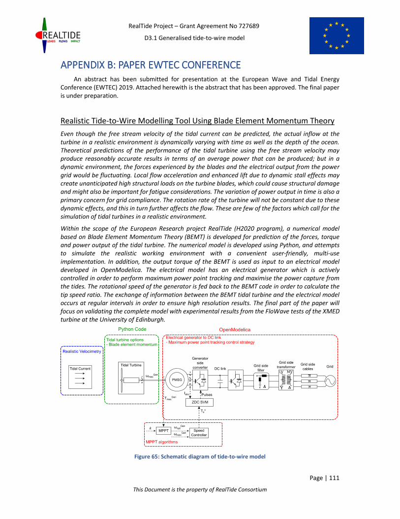
RealTide Project – Grant Agreement No 727689
D3.1 Generalised tide-to-wire model
Page | 111
This Document is the property of RealTide Consortium
APPENDIX B: PAAPPENDIX B: PAAPPENDIX B: PAAPPENDIX B: PAPER EWTEC CONFERENCEPER EWTEC CONFERENCEPER EWTEC CONFERENCEPER EWTEC CONFERENCE
An abstract has been submitted for presentation at the European Wave and Tidal Energy
Conference (EWTEC) 2019. Attached herewith is the abstract that has been approved. The final paper
is under preparation.
Realistic Tide-to-Wire Modelling Tool Using Blade Element Momentum Theory
Even though the free stream velocity of the tidal current can be predicted, the actual inflow at the
turbine in a realistic environment is dynamically varying with time as well as the depth of the ocean.
Theoretical predictions of the performance of the tidal turbine using the free stream velocity may
produce reasonably accurate results in terms of an average power that can be produced; but in a
dynamic environment, the forces experienced by the blades and the electrical output from the power
grid would be fluctuating. Local flow acceleration and enhanced lift due to dynamic stall effects may
create unanticipated high structural loads on the turbine blades, which could cause structural damage
and might also be important for fatigue considerations. The variation of power output in time is also a
primary concern for grid compliance. The rotation rate of the turbine will not be constant due to these
dynamic effects, and this in turn further affects the flow. These are few of the factors which call for the
simulation of tidal turbines in a realistic environment.
Within the scope of the European Research project RealTide (H2020 program), a numerical model
based on Blade Element Momentum Theory (BEMT) is developed for prediction of the forces, torque
and power output of the tidal turbine. The numerical model is developed using Python, and attempts
to simulate the realistic working environment with a convenient user-friendly, multi-use
implementation. In addition, the output torque of the BEMT is used as input to an electrical model
developed in OpenModelica. The electrical model has an electrical generator which is actively
controlled in order to perform maximum power point tracking and maximise the power capture from
the tides. The rotational speed of the generator is fed back to the BEMT code in order to calculate the
tip speed ratio. The exchange of information between the BEMT tidal turbine and the electrical model
occurs at regular intervals in order to ensure high resolution results. The final part of the paper will
focus on validating the complete model with experimental results from the FloWave tests of the XMED
turbine at the University of Edinburgh.
Figure 65: Schematic diagram of tide-to-wire model