Embed Size (px)
Citation preview

ADVANCED MODERN PHYSICS - Theoretical Foundations© World Scientific Publishing Co. Pte. Ltd.http://www.worldscibooks.com/physics/7555.html
January 27, 2010 10:37 WSPC/Book Trim Size for 9in x 6in V2root
Contents
Preface vii
1. Introduction 1
2. Quantum Mechanics (Revisited) 9
2.1 Linear Vector Spaces . . . . . . . . . . . . . . . . . . . . . . 9
2.1.1 Three-Dimensional Vectors . . . . . . . . . . . . . . 9
2.1.2 n-Dimensions . . . . . . . . . . . . . . . . . . . . . . 10
2.2 Hilbert Space . . . . . . . . . . . . . . . . . . . . . . . . . . 11
2.2.1 Example . . . . . . . . . . . . . . . . . . . . . . . . 11
2.2.2 Definition . . . . . . . . . . . . . . . . . . . . . . . . 12
2.2.3 Relation to Linear Vector Space . . . . . . . . . . . 13
2.2.4 Abstract State Vector . . . . . . . . . . . . . . . . . 13
2.3 Linear Hermitian Operators . . . . . . . . . . . . . . . . . . 14
2.3.1 Eigenfunctions . . . . . . . . . . . . . . . . . . . . . 15
2.3.2 Eigenstates of Position . . . . . . . . . . . . . . . . 16
2.4 Abstract Hilbert Space . . . . . . . . . . . . . . . . . . . . 18
2.4.1 Inner Product . . . . . . . . . . . . . . . . . . . . . 18
2.4.2 Completeness . . . . . . . . . . . . . . . . . . . . . . 19
2.4.3 Linear Hermitian Operators . . . . . . . . . . . . . 19
2.4.3.1 Eigenstates . . . . . . . . . . . . . . . . . . 20
2.4.3.2 Adjoint Operators . . . . . . . . . . . . . . 20
2.4.4 Schrodinger Equation . . . . . . . . . . . . . . . . . 20
2.4.4.1 Stationary States . . . . . . . . . . . . . . . 23
2.5 Measurements . . . . . . . . . . . . . . . . . . . . . . . . . 23
2.5.1 Coordinate Space . . . . . . . . . . . . . . . . . . . 23
ix

ADVANCED MODERN PHYSICS - Theoretical Foundations© World Scientific Publishing Co. Pte. Ltd.http://www.worldscibooks.com/physics/7555.html
January 27, 2010 10:37 WSPC/Book Trim Size for 9in x 6in V2root
x Advanced Modern Physics
2.5.2 Abstract Form . . . . . . . . . . . . . . . . . . . . . 25
2.5.3 Reduction of the Wave Packet . . . . . . . . . . . . 26
2.5.4 Stern-Gerlach Experiment . . . . . . . . . . . . . . 27
2.6 Quantum Mechanics Postulates . . . . . . . . . . . . . . . . 29
2.7 Many-Particle Hilbert Space . . . . . . . . . . . . . . . . . 30
2.7.1 Simple Harmonic Oscillator . . . . . . . . . . . . . . 30
2.7.2 Bosons . . . . . . . . . . . . . . . . . . . . . . . . . 31
2.7.3 Fermions . . . . . . . . . . . . . . . . . . . . . . . . 33
3. Angular Momentum 35
3.1 Translations . . . . . . . . . . . . . . . . . . . . . . . . . . 35
3.2 Rotations . . . . . . . . . . . . . . . . . . . . . . . . . . . . 37
3.3 Angular Momentum Operator . . . . . . . . . . . . . . . . 39
3.4 Eigenvalue Spectrum . . . . . . . . . . . . . . . . . . . . . . 40
3.5 Coupling of Angular Momenta . . . . . . . . . . . . . . . . 46
3.6 Recoupling . . . . . . . . . . . . . . . . . . . . . . . . . . . 53
3.7 Irreducible Tensor Operators . . . . . . . . . . . . . . . . . 55
3.8 The Wigner-Eckart Theorem . . . . . . . . . . . . . . . . . 57
3.9 Finite Rotations . . . . . . . . . . . . . . . . . . . . . . . . 59
3.9.1 Properties . . . . . . . . . . . . . . . . . . . . . . . 61
3.9.2 Tensor Operators . . . . . . . . . . . . . . . . . . . 63
3.9.3 Wigner-Eckart Theorem (Completed) . . . . . . . . 64
3.10 Tensor Products . . . . . . . . . . . . . . . . . . . . . . . . 65
3.11 Vector Model . . . . . . . . . . . . . . . . . . . . . . . . . . 66
4. Scattering Theory 69
4.1 Interaction Picture . . . . . . . . . . . . . . . . . . . . . . . 69
4.2 Adiabatic Approach . . . . . . . . . . . . . . . . . . . . . . 70
4.3 U -Operator . . . . . . . . . . . . . . . . . . . . . . . . . . . 72
4.4 U -Operator for Finite Times . . . . . . . . . . . . . . . . . 76
4.5 The S-Matrix . . . . . . . . . . . . . . . . . . . . . . . . . . 77
4.6 Time-Independent Analysis . . . . . . . . . . . . . . . . . . 79
4.7 Scattering State . . . . . . . . . . . . . . . . . . . . . . . . 83
4.8 Transition Rate . . . . . . . . . . . . . . . . . . . . . . . . . 86
4.9 Unitarity . . . . . . . . . . . . . . . . . . . . . . . . . . . . 89
4.10 Example: Potential Scattering . . . . . . . . . . . . . . . . 90
4.10.1 Green’s Function (Propagator) . . . . . . . . . . . . 90
4.10.2 Scattering Wave Function . . . . . . . . . . . . . . . 92

ADVANCED MODERN PHYSICS - Theoretical Foundations© World Scientific Publishing Co. Pte. Ltd.http://www.worldscibooks.com/physics/7555.html
January 27, 2010 10:37 WSPC/Book Trim Size for 9in x 6in V2root
Contents xi
4.10.3 T-matrix . . . . . . . . . . . . . . . . . . . . . . . . 93
4.10.4 Cross Section . . . . . . . . . . . . . . . . . . . . . . 93
4.10.5 Unitarity . . . . . . . . . . . . . . . . . . . . . . . . 94
5. Lagrangian Field Theory 95
5.1 Particle Mechanics . . . . . . . . . . . . . . . . . . . . . . . 96
5.1.1 Hamilton’s Principle . . . . . . . . . . . . . . . . . . 96
5.1.2 Lagrange’s Equations . . . . . . . . . . . . . . . . . 97
5.1.3 Hamiltonian . . . . . . . . . . . . . . . . . . . . . . 98
5.2 Continuum Mechanics (String–a Review) . . . . . . . . . . 101
5.2.1 Lagrangian Density . . . . . . . . . . . . . . . . . . 101
5.2.2 Hamilton’s Principle . . . . . . . . . . . . . . . . . . 102
5.2.3 Lagrange’s Equation . . . . . . . . . . . . . . . . . . 103
5.2.4 Two-Vectors . . . . . . . . . . . . . . . . . . . . . . 103
5.2.5 Momentum Density . . . . . . . . . . . . . . . . . . 104
5.2.6 Hamiltonian Density . . . . . . . . . . . . . . . . . . 104
5.3 Quantization . . . . . . . . . . . . . . . . . . . . . . . . . . 104
5.3.1 Particle Mechanics . . . . . . . . . . . . . . . . . . . 104
5.3.2 Continuum Mechanics (String) . . . . . . . . . . . . 106
5.4 Relativistic Field Theory . . . . . . . . . . . . . . . . . . . 108
5.4.1 Scalar Field . . . . . . . . . . . . . . . . . . . . . . . 109
5.4.2 Stress Tensor . . . . . . . . . . . . . . . . . . . . . . 111
5.4.3 Dirac Field . . . . . . . . . . . . . . . . . . . . . . . 117
5.4.4 Noether’s Theorem . . . . . . . . . . . . . . . . . . 120
5.4.4.1 Normal-Ordered Current . . . . . . . . . . 122
5.4.5 Electromagnetic Field . . . . . . . . . . . . . . . . . 123
5.4.6 Interacting Fields (Dirac-Scalar) . . . . . . . . . . . 123
6. Symmetries 125
6.1 Lorentz Invariance . . . . . . . . . . . . . . . . . . . . . . . 125
6.2 Rotational Invariance . . . . . . . . . . . . . . . . . . . . . 126
6.3 Internal Symmetries . . . . . . . . . . . . . . . . . . . . . . 127
6.3.1 Isospin–SU(2) . . . . . . . . . . . . . . . . . . . . . 127
6.3.1.1 Isovector . . . . . . . . . . . . . . . . . . . 127
6.3.1.2 Isospinor . . . . . . . . . . . . . . . . . . . 131
6.3.1.3 Transformation Law . . . . . . . . . . . . . 133
6.3.2 Lie Groups . . . . . . . . . . . . . . . . . . . . . . . 134
6.3.3 Sakata Model–SU(3) . . . . . . . . . . . . . . . . . . 138

ADVANCED MODERN PHYSICS - Theoretical Foundations© World Scientific Publishing Co. Pte. Ltd.http://www.worldscibooks.com/physics/7555.html
January 27, 2010 10:37 WSPC/Book Trim Size for 9in x 6in V2root
xii Advanced Modern Physics
6.3.3.1 Dirac Triplet . . . . . . . . . . . . . . . . . 139
6.3.3.2 Scalar Octet . . . . . . . . . . . . . . . . . 141
6.3.3.3 Interacting Fields (Dirac-Scalar) . . . . . . 142
6.4 Phase Invariance . . . . . . . . . . . . . . . . . . . . . . . . 142
6.4.1 Global Phase Invariance . . . . . . . . . . . . . . . . 142
6.4.2 Local Phase Invariance . . . . . . . . . . . . . . . . 143
6.5 Yang-Mills Theories . . . . . . . . . . . . . . . . . . . . . . 145
6.6 Chiral Symmetry . . . . . . . . . . . . . . . . . . . . . . . . 151
6.6.1 σ-Model . . . . . . . . . . . . . . . . . . . . . . . . . 156
6.6.2 Spontaneous Symmetry Breaking . . . . . . . . . . 158
6.7 Lorentz Transformations . . . . . . . . . . . . . . . . . . . 162
7. Feynman Rules 163
7.1 Wick’s Theorem . . . . . . . . . . . . . . . . . . . . . . . . 164
7.2 Example (Dirac-Scalar) . . . . . . . . . . . . . . . . . . . . 171
7.2.1 Scattering Amplitudes . . . . . . . . . . . . . . . . . 172
7.2.2 Self-Energies . . . . . . . . . . . . . . . . . . . . . . 175
7.2.3 Vacuum Amplitude . . . . . . . . . . . . . . . . . . 176
7.3 Feynman Diagrams . . . . . . . . . . . . . . . . . . . . . . 177
7.4 Feynman Rules . . . . . . . . . . . . . . . . . . . . . . . . . 180
7.5 Cancellation of Disconnected Diagrams . . . . . . . . . . . 182
7.6 Mass Renormalization . . . . . . . . . . . . . . . . . . . . . 185
8. Quantum Electrodynamics (QED) 187
8.1 Classical Theory . . . . . . . . . . . . . . . . . . . . . . . . 187
8.2 Hamiltonian . . . . . . . . . . . . . . . . . . . . . . . . . . 188
8.3 Quantization . . . . . . . . . . . . . . . . . . . . . . . . . . 189
8.4 Photon Propagator . . . . . . . . . . . . . . . . . . . . . . . 191
8.5 Second-Order Processes . . . . . . . . . . . . . . . . . . . . 196
8.5.1 Scattering Amplitudes . . . . . . . . . . . . . . . . . 196
8.5.2 Self-Energies . . . . . . . . . . . . . . . . . . . . . . 198
8.6 QED With Two Leptons . . . . . . . . . . . . . . . . . . . 200
8.7 Cross Sections . . . . . . . . . . . . . . . . . . . . . . . . . 200
8.7.1 e− + µ− → e− + µ− . . . . . . . . . . . . . . . . . . 200
8.7.1.1 Scattering Amplitude . . . . . . . . . . . . 201
8.7.1.2 Cross Section . . . . . . . . . . . . . . . . . 201
8.7.1.3 Traces . . . . . . . . . . . . . . . . . . . . . 205
8.7.1.4 Cross Section (Continued) . . . . . . . . . . 206
ADVANCED MODERN PHYSICS - Theoretical Foundations© World Scientific Publishing Co. Pte. Ltd.http://www.worldscibooks.com/physics/7555.html
January 27, 2010 10:37 WSPC/Book Trim Size for 9in x 6in V2root
Contents xiii
8.7.1.5 Limiting Cases . . . . . . . . . . . . . . . . 208
8.7.1.6 Mo/ ller Scattering . . . . . . . . . . . . . . 209
8.7.2 e+ + e− → µ+ + µ− . . . . . . . . . . . . . . . . . . 210
8.7.2.1 Scattering Amplitude . . . . . . . . . . . . 210
8.7.2.2 Cross Section . . . . . . . . . . . . . . . . . 211
8.7.2.3 Limiting Cases . . . . . . . . . . . . . . . . 214
8.7.2.4 Colliding Beams . . . . . . . . . . . . . . . 214
8.8 QED in External Field . . . . . . . . . . . . . . . . . . . . 214
8.8.1 Nuclear Coulomb Field . . . . . . . . . . . . . . . . 216
8.8.2 Bremsstrahlung . . . . . . . . . . . . . . . . . . . . 217
8.8.3 Pair Production . . . . . . . . . . . . . . . . . . . . 218
8.9 Scattering Operator Sext1 in Order e3 . . . . . . . . . . . . . 219
8.10 Feynman Rules for QED . . . . . . . . . . . . . . . . . . . 221
8.10.1 General Scattering Operator . . . . . . . . . . . . . 221
8.10.2 Feynman Diagrams . . . . . . . . . . . . . . . . . . 222
8.10.3 Feynman Rules . . . . . . . . . . . . . . . . . . . . . 223
8.10.3.1 Coordinate Space . . . . . . . . . . . . . . 223
8.10.3.2 Momentum Space . . . . . . . . . . . . . . 223
9. Higher-Order Processes 225
9.1 Example–Scattering in External Field . . . . . . . . . . . . 225
9.1.1 Feynman Diagrams . . . . . . . . . . . . . . . . . . 226
9.1.2 First-Order . . . . . . . . . . . . . . . . . . . . . . . 226
9.1.3 Vertex Insertion . . . . . . . . . . . . . . . . . . . . 226
9.1.4 Vacuum Polarization . . . . . . . . . . . . . . . . . 226
9.1.5 Self-Energy Insertions . . . . . . . . . . . . . . . . . 227
9.2 Ward’s Identity . . . . . . . . . . . . . . . . . . . . . . . . . 228
9.3 Electron Self-Energy . . . . . . . . . . . . . . . . . . . . . . 228
9.3.1 General Form . . . . . . . . . . . . . . . . . . . . . 229
9.3.2 Evaluation . . . . . . . . . . . . . . . . . . . . . . . 230
9.3.3 Mass Renormalization . . . . . . . . . . . . . . . . . 232
9.4 Vertex . . . . . . . . . . . . . . . . . . . . . . . . . . . . . . 234
9.4.1 General Form . . . . . . . . . . . . . . . . . . . . . 234
9.4.2 Ward’s Identity . . . . . . . . . . . . . . . . . . . . 235
9.4.3 Evaluation . . . . . . . . . . . . . . . . . . . . . . . 236
9.4.4 The Constant L . . . . . . . . . . . . . . . . . . . . 238
9.4.5 The Infrared Problem . . . . . . . . . . . . . . . . . 239
9.4.6 Schwinger Moment . . . . . . . . . . . . . . . . . . . 240
9.5 External Lines and Wavefunction Renormalization . . . . . 243

ADVANCED MODERN PHYSICS - Theoretical Foundations© World Scientific Publishing Co. Pte. Ltd.http://www.worldscibooks.com/physics/7555.html
January 27, 2010 10:37 WSPC/Book Trim Size for 9in x 6in V2root
xiv Advanced Modern Physics
9.5.1 Cancellation of Divergences . . . . . . . . . . . . . . 247
9.6 Vacuum Polarization . . . . . . . . . . . . . . . . . . . . . . 247
9.6.1 Evaluation . . . . . . . . . . . . . . . . . . . . . . . 248
9.6.2 General Form . . . . . . . . . . . . . . . . . . . . . 249
9.6.3 Limiting Cases . . . . . . . . . . . . . . . . . . . . . 250
9.6.4 Insertion . . . . . . . . . . . . . . . . . . . . . . . . 250
9.6.5 Charge Renormalization . . . . . . . . . . . . . . . . 252
9.6.6 Charge Strength . . . . . . . . . . . . . . . . . . . . 254
9.7 Renormalization Theory . . . . . . . . . . . . . . . . . . . . 255
9.7.1 Proper Self-Energies . . . . . . . . . . . . . . . . . . 255
9.7.2 Proper Vertex . . . . . . . . . . . . . . . . . . . . . 256
9.7.3 Ward’s Identity . . . . . . . . . . . . . . . . . . . . 257
9.7.4 Ward’s Vertex Construct . . . . . . . . . . . . . . . 259
9.7.5 Finite Parts . . . . . . . . . . . . . . . . . . . . . . 260
9.7.6 Proof of Renormalization . . . . . . . . . . . . . . . 262
9.7.7 The Renormalization Group . . . . . . . . . . . . . 264
10. Path Integrals 265
10.1 Non-Relativistic Quantum Mechanics with One Degree of
Freedom . . . . . . . . . . . . . . . . . . . . . . . . . . . . . 265
10.1.1 General Relations . . . . . . . . . . . . . . . . . . . 266
10.1.2 Infinitesimals . . . . . . . . . . . . . . . . . . . . . . 268
10.1.3 Transition Amplitude and Path Integral . . . . . . . 270
10.1.4 Classical Limit . . . . . . . . . . . . . . . . . . . . . 272
10.1.5 Superposition . . . . . . . . . . . . . . . . . . . . . . 272
10.1.6 Matrix Elements . . . . . . . . . . . . . . . . . . . . 273
10.1.7 Crucial Theorem of Abers and Lee . . . . . . . . . . 275
10.1.8 Functional Derivative . . . . . . . . . . . . . . . . . 276
10.1.9 Generating Functional . . . . . . . . . . . . . . . . . 279
10.2 Many Degrees of Freedom . . . . . . . . . . . . . . . . . . . 279
10.2.1 Gaussian Integrals . . . . . . . . . . . . . . . . . . . 280
10.3 Field Theory . . . . . . . . . . . . . . . . . . . . . . . . . . 282
10.3.1 Fields as Coordinates . . . . . . . . . . . . . . . . . 282
10.3.2 Measure . . . . . . . . . . . . . . . . . . . . . . . . . 283
10.3.3 Generating Functional . . . . . . . . . . . . . . . . . 283
10.3.4 Convergence . . . . . . . . . . . . . . . . . . . . . . 283
10.3.4.1 Euclidicity Postulate . . . . . . . . . . . . . 283
10.3.4.2 Adiabatic Damping . . . . . . . . . . . . . 284
10.4 Scalar Field . . . . . . . . . . . . . . . . . . . . . . . . . . . 285
ADVANCED MODERN PHYSICS - Theoretical Foundations© World Scientific Publishing Co. Pte. Ltd.http://www.worldscibooks.com/physics/7555.html
January 27, 2010 10:37 WSPC/Book Trim Size for 9in x 6in V2root
Contents xv
10.4.1 Generating Functional for Free Scalar Field . . . . . 285
10.4.1.1 Applications . . . . . . . . . . . . . . . . . 287
10.4.2 Interactions . . . . . . . . . . . . . . . . . . . . . . . 289
10.5 Fermions . . . . . . . . . . . . . . . . . . . . . . . . . . . . 290
10.5.1 Grassmann Algebra . . . . . . . . . . . . . . . . . . 290
10.5.2 Functional Derivative . . . . . . . . . . . . . . . . . 291
10.5.3 Functional Integration . . . . . . . . . . . . . . . . . 291
10.5.4 Integrals . . . . . . . . . . . . . . . . . . . . . . . . 292
10.5.5 Basic Results . . . . . . . . . . . . . . . . . . . . . . 292
10.5.6 Generating Functional for Free Dirac Field . . . . . 294
10.5.6.1 Applications . . . . . . . . . . . . . . . . . 296
10.5.7 Interactions (Dirac-Scalar) . . . . . . . . . . . . . . 297
10.6 Electromagnetic Field . . . . . . . . . . . . . . . . . . . . . 298
11. Canonical Transformations for Quantum Systems 299
11.1 Interacting Bose System . . . . . . . . . . . . . . . . . . . . 300
11.1.1 Pseudopotential . . . . . . . . . . . . . . . . . . . . 300
11.1.2 Special Role of the Ground State . . . . . . . . . . . 301
11.1.3 Effective Hamiltonian . . . . . . . . . . . . . . . . . 302
11.1.4 Bogoliubov Transformation . . . . . . . . . . . . . . 303
11.1.5 Discussion of Results . . . . . . . . . . . . . . . . . 305
11.1.5.1 Excitation Spectrum . . . . . . . . . . . . . 305
11.1.5.2 Depletion . . . . . . . . . . . . . . . . . . . 306
11.1.5.3 Ground-State Energy . . . . . . . . . . . . 308
11.1.6 Superfluid 4He . . . . . . . . . . . . . . . . . . . . . 309
11.2 Superconductors . . . . . . . . . . . . . . . . . . . . . . . . 309
11.2.1 Cooper Pairs . . . . . . . . . . . . . . . . . . . . . . 309
11.2.2 Bogoliubov-Valatin Transformation . . . . . . . . . 310
11.2.2.1 Pairing . . . . . . . . . . . . . . . . . . . . 310
11.2.2.2 Thermodynamic Potential . . . . . . . . . . 311
11.2.2.3 Wick’s Theorem . . . . . . . . . . . . . . . 312
11.2.2.4 Diagonalization of K0 . . . . . . . . . . . . 314
11.2.2.5 Gap Equation . . . . . . . . . . . . . . . . 316
11.2.3 Discussion of Results . . . . . . . . . . . . . . . . . 316
11.2.3.1 Particle Number . . . . . . . . . . . . . . . 316
11.2.3.2 Ground-State Thermodynamic Potential . . 317
11.2.3.3 Ground-State Energy . . . . . . . . . . . . 318
11.2.3.4 Excitation Spectrum . . . . . . . . . . . . . 318
11.2.3.5 Momentum Operator . . . . . . . . . . . . 319

ADVANCED MODERN PHYSICS - Theoretical Foundations© World Scientific Publishing Co. Pte. Ltd.http://www.worldscibooks.com/physics/7555.html
January 27, 2010 10:37 WSPC/Book Trim Size for 9in x 6in V2root
xvi Advanced Modern Physics
11.2.3.6 Quasiparticle Spectrum . . . . . . . . . . . 319
11.2.3.7 Calculation of the Energy Gap ∆ . . . . . . 320
11.2.3.8 Quasiparticle Interactions . . . . . . . . . . 322
12. Problems 323
Appendix A Multipole Analysis of the Radiation Field 369
A.1 Vector Spherical Harmonics . . . . . . . . . . . . . . . . . . 370
A.2 Plane-Wave Expansion . . . . . . . . . . . . . . . . . . . . 373
A.3 Transition Rate . . . . . . . . . . . . . . . . . . . . . . . . . 375
A.4 Arbitrary Photon Direction . . . . . . . . . . . . . . . . . . 379
Appendix B Functions of a Complex Variable 383
B.1 Convergence . . . . . . . . . . . . . . . . . . . . . . . . . . 383
B.2 Analytic Functions . . . . . . . . . . . . . . . . . . . . . . . 383
B.3 Integration . . . . . . . . . . . . . . . . . . . . . . . . . . . 384
B.4 Cauchy’s Theorem . . . . . . . . . . . . . . . . . . . . . . . 385
B.5 Cauchy’s Integral . . . . . . . . . . . . . . . . . . . . . . . . 385
B.6 Taylor’s Theorem . . . . . . . . . . . . . . . . . . . . . . . 387
B.7 Laurent Series . . . . . . . . . . . . . . . . . . . . . . . . . 387
B.8 Theory of Residues . . . . . . . . . . . . . . . . . . . . . . . 387
B.9 Zeros of an Analytic Function . . . . . . . . . . . . . . . . . 389
B.10 Analytic Continuation . . . . . . . . . . . . . . . . . . . . . 389
B.10.1 Standard Method . . . . . . . . . . . . . . . . . . . 390
B.10.2 Uniqueness . . . . . . . . . . . . . . . . . . . . . . . 391
Appendix C Electromagnetic Field 393
C.1 Lagrangian Field Theory . . . . . . . . . . . . . . . . . . . 394
C.2 Stress Tensor . . . . . . . . . . . . . . . . . . . . . . . . . . 395
C.3 Free Fields . . . . . . . . . . . . . . . . . . . . . . . . . . . 395
C.4 Quantization . . . . . . . . . . . . . . . . . . . . . . . . . . 397
C.5 Commutation Relations . . . . . . . . . . . . . . . . . . . . 399
C.6 Interaction With External Current . . . . . . . . . . . . . . 401
C.6.1 Hamiltonian . . . . . . . . . . . . . . . . . . . . . . 402
C.6.2 Quantization . . . . . . . . . . . . . . . . . . . . . . 404
Appendix D Irreducible Representations of SU(n) 407
D.1 Young Tableaux and Young Operators . . . . . . . . . . . . 409

ADVANCED MODERN PHYSICS - Theoretical Foundations© World Scientific Publishing Co. Pte. Ltd.http://www.worldscibooks.com/physics/7555.html
January 27, 2010 10:37 WSPC/Book Trim Size for 9in x 6in V2root
Contents xvii
D.2 Adjoint Representation . . . . . . . . . . . . . . . . . . . . 410
D.3 Dimension of the Representation . . . . . . . . . . . . . . . 412
D.4 Outer Product . . . . . . . . . . . . . . . . . . . . . . . . . 412
D.5 SU(n-1) Content of SU(n) . . . . . . . . . . . . . . . . . . . 413
D.6 Some Examples . . . . . . . . . . . . . . . . . . . . . . . . . 414
D.6.1 Angular Momentum–SU(2) . . . . . . . . . . . . . . 414
D.6.2 Sakata Model–SU(3) . . . . . . . . . . . . . . . . . . 415
D.6.3 Giant Resonances–SU(4) . . . . . . . . . . . . . . . 417
Appendix E Lorentz Transformations in Quantum Field Theory 419
E.1 Scalar Field . . . . . . . . . . . . . . . . . . . . . . . . . . . 420
E.1.1 States . . . . . . . . . . . . . . . . . . . . . . . . . . 420
E.1.2 Lorentz Transformation . . . . . . . . . . . . . . . . 422
E.1.3 Generators . . . . . . . . . . . . . . . . . . . . . . . 423
E.1.4 Commutation Rules . . . . . . . . . . . . . . . . . . 426
E.2 Dirac Field . . . . . . . . . . . . . . . . . . . . . . . . . . . 427
E.2.1 Lorentz Transformation . . . . . . . . . . . . . . . . 427
Appendix F Green’s Functions and Other Singular Functions 429
F.1 Commutator at Unequal Times . . . . . . . . . . . . . . . . 429
F.2 Green’s Functions . . . . . . . . . . . . . . . . . . . . . . . 434
F.2.1 Boundary Conditions . . . . . . . . . . . . . . . . . 437
F.3 Time-Ordered Products . . . . . . . . . . . . . . . . . . . . 439
F.3.1 Scalar Field . . . . . . . . . . . . . . . . . . . . . . . 439
F.3.2 Electromagnetic Field . . . . . . . . . . . . . . . . . 440
F.3.3 Dirac Field . . . . . . . . . . . . . . . . . . . . . . . 440
F.3.4 Vector Field . . . . . . . . . . . . . . . . . . . . . . 442
Appendix G Dimensional Regularization 443
G.1 Dirichlet Integral . . . . . . . . . . . . . . . . . . . . . . . . 444
G.2 Basic Relation . . . . . . . . . . . . . . . . . . . . . . . . . 445
G.3 Complex n-plane . . . . . . . . . . . . . . . . . . . . . . . . 446
G.4 Algebra . . . . . . . . . . . . . . . . . . . . . . . . . . . . . 447
G.5 Lorentz Metric . . . . . . . . . . . . . . . . . . . . . . . . . 448
G.6 γ-Matrix Algebra . . . . . . . . . . . . . . . . . . . . . . . . 449
G.7 Examples . . . . . . . . . . . . . . . . . . . . . . . . . . . . 449
G.7.1 Convergent Momentum Integrals . . . . . . . . . . . 450
G.7.2 Vacuum Tadpoles . . . . . . . . . . . . . . . . . . . 450

ADVANCED MODERN PHYSICS - Theoretical Foundations© World Scientific Publishing Co. Pte. Ltd.http://www.worldscibooks.com/physics/7555.html
January 27, 2010 10:37 WSPC/Book Trim Size for 9in x 6in V2root
xviii Advanced Modern Physics
G.7.3 Vacuum Polarization . . . . . . . . . . . . . . . . . 450
Appendix H Path Integrals and the Electromagnetic Field 453
H.1 Faddeev-Popov Identity . . . . . . . . . . . . . . . . . . . . 453
H.2 Application . . . . . . . . . . . . . . . . . . . . . . . . . . . 455
H.3 Generating Functional . . . . . . . . . . . . . . . . . . . . . 457
H.4 Ghosts . . . . . . . . . . . . . . . . . . . . . . . . . . . . . 458
H.5 Photon Propagator . . . . . . . . . . . . . . . . . . . . . . . 458
Appendix I Metric Conversion 461
Bibliography 463
Index 467

ADVANCED MODERN PHYSICS - Theoretical Foundations© World Scientific Publishing Co. Pte. Ltd.http://www.worldscibooks.com/physics/7555.html
January 27, 2010 10:37 WSPC/Book Trim Size for 9in x 6in V2root
Preface
World Scientific Publishing Company recently published my book entitled
Introduction to Modern Physics: Theoretical Foundations. The book is
aimed at the very best students, with a goal of exposing them to the foun-
dations and frontiers of today’s physics. Typically, students have to wade
through several courses to see many of these topics, and I wanted them to
have some idea of where they were going, and how things fit together, as
they went along. Hopefully, they will then see more inter-relationships, and
get more original insights, as they progress. The book assumes the reader
has had a good one-year, calculus-based freshman physics course, along
with a good one-year course in calculus. While it is assumed that mathe-
matical skills will continue to develop, several appendices are included to
bring the reader up to speed on any additional mathematics required at the
outset. With very few exceptions, the reader should then find the material
to be self-contained. Many problems are included, some for each chapter.
Although the book is designed so that one can, in principle, read and follow
the text without doing any of the problems, the reader is strongly urged
to attempt as many of them as possible in order to obtain some confidence
in his or her understanding of the basics of modern physics and to hone
working skills.
After completing that book, it occurred to me that a second volume
could be prepared that would significantly extend the coverage, while fur-
thering the stated goals. The ground rules would be that anything covered
in the text and appendices of the first volume would be fair game, while
anything covered in the problems would first be re-summarized. Those few
results quoted without proof in Vol. I would now be derived. The topics
chosen would be those of wide applicability in all areas of physics. Again,
an important goal would be to keep the entire coverage self-contained. The
vii
ADVANCED MODERN PHYSICS - Theoretical Foundations© World Scientific Publishing Co. Pte. Ltd.http://www.worldscibooks.com/physics/7555.html
January 27, 2010 10:37 WSPC/Book Trim Size for 9in x 6in V2root
viii Preface
present book is the outcome of those musings. All of the material in this
book is taken from course lectures given over the years by the author at
either Stanford University or the College of William and Mary.
Quantum mechanics is first reformulated in abstract Hilbert space,
which allows one to focus on the general structure of the theory. The book
then covers the following topics: angular momentum, scattering theory, la-
grangian field theory, symmetries, Feynman rules, quantum electrodynam-
ics, path integrals, and canonical transformations for quantum systems.
Several appendices are included with important details. When finished,
the reader should have an elementary working knowledge in the principal
areas of theoretical physics of the twentieth century. With this overview in
hand, development in depth and reach in these areas can then be obtained
from more advanced physics courses.
I was again delighted when World Scientific Publishing Company, which
had done an exceptional job with four of my previous books, showed enthu-
siasm for publishing this new one. I would like to thank Dr. K. K. Phua,
Executive Chairman of World Scientific Publishing Company, and my ed-
itor Ms. Lakshmi Narayanan, for their help and support on this project.
I am greatly indebted to my colleagues Paolo Amore and Alfredo Aranda
for their reading of the manuscript.
John Dirk Walecka
Governor’s Distinguished CEBAF
Professor of Physics, emeritus
College of William and Mary
Williamsburg, Virginia
December 1, 2009

ADVANCED MODERN PHYSICS - Theoretical Foundations© World Scientific Publishing Co. Pte. Ltd.http://www.worldscibooks.com/physics/7555.html
January 27, 2010 10:37 WSPC/Book Trim Size for 9in x 6in V2root
Chapter 1
Introduction
The goal of this book is to provide an extension of the previous book Intro-
duction to Modern Physics: Theoretical Foundations, refered to as Vol. I.
That volume develops the underlying concepts in twentieth-century physics:
quantum mechanics, special relativity, and general relativity. Included in it
are applications in atomic, nuclear, particle, and condensed matter physics.
It is assumed in Vol. I that readers have had a good calculus-based intro-
ductory physics course together with a good course in calculus. Several
appendices then provide sufficient background so that, with very few ex-
ceptions, the presentation is self-contained. Many of the topics covered in
that work are more advanced than in the usual introductory modern physics
books. It was the author’s intention to provide the best students with an
overview of the subject, so that they are aware of the overall picture and
can see how things fit together as they progress.
As projected in Vol. I, it is now assumed that mathematical skills have
continued to develop. In this volume, readers are expected to be familiar
with multi-variable calculus, in particular, with multiple integrals. It is
also assumed that readers have some familiarity with the essentials of linear
algebra. An appendix is included here on functions of a complex variable,
since complex integration plays a key role in the analysis. The ground
rules now are that anything covered in the text and appendices in Vol. I is
assumed to be mastered, while anything covered in the problems in Vol. I
will be re-summarized. Within this framework, readers should again find
Vol. II to be self-contained.
There are over 175 problems in this book, some after each chapter and
appendix. The problems are not meant to baffle the reader, but rather
to enhance the coverage and to provide exercises on working skills. The
problems for the most part are not difficult, and in most cases the steps
1
ADVANCED MODERN PHYSICS - Theoretical Foundations© World Scientific Publishing Co. Pte. Ltd.http://www.worldscibooks.com/physics/7555.html
January 27, 2010 10:37 WSPC/Book Trim Size for 9in x 6in V2root
2 Advanced Modern Physics
are clearly laid out. Those problems that may involve somewhat more
algebra are so noted. The reader is urged to attempt as many problems as
possible in order to obtain some confidence in his or her understanding of
the framework of modern theoretical physics.
In chapter 2 we revisit quantum mechanics and reformulate the the-
ory in terms of linear hermitian operators acting in an abstract Hilbert
space. Once we know how to compute inner products, and have the com-
pleteness relation, we understand the essentials of operating in this space.
The basic elements of measurement theory are also covered. We are then
able to present quantum mechanics in terms of a set of postulates within
this framework. The quantum fields of Vol. I are operators acting in the
abstract many-particle Hilbert space.
Chapter 3 is devoted to the quantum theory of angular momentum, and
this subject is covered in some depth. There are a variety of motivations
here: this theory governs the behavior of any isolated, finite quantum me-
chanical system and lies at the heart of most of the applications in Vol. I;1
it provides a detailed illustration of the consequences of a continuous sym-
metry in quantum mechanics, in this case the very deep symmetry of the
isotropy of space; furthermore, it provides an extensive introduction to the
theory of Lie groups, here the special unitary group in two dimensions
SU(2), which finds wide applicability in internal symmetries. An appendix
explores the use of angular momentum theory in the multipole analysis of
the radiation field, which is applicable to transitions in any finite quantum
mechanical system.
Chapter 4 is devoted to scattering theory. The Schrodinger equation
is solved in terms of a time-development operator in the abstract Hilbert
space, and the scattering operator is identified. The interaction is turned
on and off “adiabatically”, which allows a simple construction of initial and
final states, and the S-matrix elements then follow immediately. Although
inappropriate for developing a covariant scattering analysis, the time inte-
grations in the scattering operator can be explicitly performed and contact
made with time-independent scattering theory. It is shown how adiabatic
damping puts the correct boundary conditions into the propagators. A
general expression is derived for the quantum mechanical transition rate.
Non-relativistic scattering from a static potential provides a nice example
of the time-independent analysis. If the time is left in the scattering op-
erator, one has a basis for the subsequent analysis in terms of Feynman
1For example, here we validate the “vector model” used there.

ADVANCED MODERN PHYSICS - Theoretical Foundations© World Scientific Publishing Co. Pte. Ltd.http://www.worldscibooks.com/physics/7555.html
January 27, 2010 10:37 WSPC/Book Trim Size for 9in x 6in V2root
Introduction 3
diagrams and Feynman rules. The tools developed in this chapter allow
one to analyze any scattering or reaction process in quantum mechanics.
Lagrangian field theory provides the dynamical framework for a consis-
tent, covariant, quantum mechanical description of many interacting parti-
cles, and this is the topic in chapter 4. We first review classical lagrangian
particle mechanics, and then classical lagrangian continuum mechanics, us-
ing our paradigm of the transverse planar oscillations of a string. The string
mechanics can be expressed in terms of “two-vectors” (x, ict) where c is the
sound velocity in the string. We then discuss the quantization of these
classical mechanical systems obtained by imposing canonical quantization
relations on the operators in the abstract Hilbert space.
The appending of two additional spatial dimensions to obtain four-
vectors (x, ict), where c is now the speed of light, leads immediately to a
covariant, continuum lagrangian mechanics for a scalar field in Minkowski
space, which is then quantized with the same procedure used for the string.
We develop a covariant, continuum lagrangian mechanics for the Dirac field,
and discuss how anticommutation relations must be imposed when quantiz-
ing in this case. A general expression is derived for the energy-momentum
tensor, and Noether’s theorem is proven, which states that for every contin-
uous symmetry of the lagrangian density there is an associated conserved
current. A full appendix is dedicated to the lagrangian field theory of the
electromagnetic field.
Symmetries play a central role in developing covariant lagrangian densi-
ties for various interacting systems, and chapter 6 is devoted to symmetries.
The discussion starts with spatial rotations and the internal symmetry of
isospin, and it builds on the analysis of SU(2) in chapter 3. Here isospin
is developed in terms of global SU(2) transformations of the nucleon field
ψ = (ψp, ψn). The internal symmetry is generalized to SU(3) within the
framework of the Sakata model with a baryon field ψ = (ψp, ψn, ψΛ).2
It is also shown in chapter 6 how the imposition of invariance under local
phase transformations of the charged Dirac field, where the transformation
parameter depends on the space-time point x, necessitates the introduction
of a photon (gauge) field Aµ(x) and leads to quantum electrodynamics
(QED), the most accurate theory known. Yang-Mills theory, which extends
this idea to invariance under local internal symmetry transformations of
the Dirac field, and necessitates the introduction of corresponding gauge
bosons, is developed in detail. These gauge bosons must be massless, and to
2Wigner’s supermultiplet theory based on internal SU(4) transformations of the nu-cleon field ψ = (ψp↑, ψp↓, ψn↑, ψn↓) is also touched on.

ADVANCED MODERN PHYSICS - Theoretical Foundations© World Scientific Publishing Co. Pte. Ltd.http://www.worldscibooks.com/physics/7555.html
January 27, 2010 10:37 WSPC/Book Trim Size for 9in x 6in V2root
4 Advanced Modern Physics
understand the very successful physical application of Yang-Mills theories,
it is necessary to understand how mass is generated in relativistic quantum
field theories.3
We do this within the framework of the σ-model, a very simple model
which has had a profound effect on the development of modern physics.
A massless Dirac field has an additional chiral invariance under a global
transformation that also mixes the components of the Dirac field. The cor-
responding conserved axial-vector current, which augments the conserved
vector current arising from global isospin invariance, corresponds closely to
what is observed experimentally in the weak interactions. The σ-model ex-
tends the massless Dirac lagrangian through a chiral-invariant interaction
with a pion and scalar field (π, σ). A choice of shape of the chiral-invariant
meson potential V(π2+σ2) then leads to a vacuum expectation value for the
scalar field that gives rise to a mass for the Dirac particle while maintaining
chiral invariance of the lagrangian. This spontaneous symmetry breaking il-
lustrates how observed states do not necessarily reflect the symmetry of the
underlying lagrangian. Generating mass through the expectation value of
a scalar field, in one way or another, now underlies most modern theories
of particle interactions.4
The most fundamental symmetry in nature is Lorentz invariance. One
must obtain the same physics in any Lorentz frame. The Lorentz transfor-
mation properties of the scalar and Dirac fields are detailed in an appendix.
Some very useful tools are provided in another appendix devoted to the ir-
reducible representations of SU(n).
Chapter 7 is concerned with the derivation of the Feynman rules, and to
focus on the method, they are developed for the simplest theory of a Dirac
particle interacting with a neutral, massive, scalar field. Wick’s theorem
is proven. This allows one to convert a time-ordered product of fields in
the interaction picture, where the time dependence is that of free fields,
into a normal-ordered product where the destruction operators sit to the
right of the creation operators for all times. It is the time-ordered prod-
uct that occurs naturally in the scattering operator, and it is the normal-
ordered product from which it is straightforward to compute any required
matrix elements. Wick’s theorem introduces the vacuum expectation value
3Both quantum chromodynamics (QCD) and the Standard Model of electroweak in-teractions are Yang-Mills theories built on internal symmetry groups, the former on aninternal color SU(3)C symmetry and the latter on an internal weak SU(2)W
⊗
U(1)W .4In the Standard Model, it provides the basis for the “Higgs mechanism” (see, for
example, [Walecka (2004)]).

ADVANCED MODERN PHYSICS - Theoretical Foundations© World Scientific Publishing Co. Pte. Ltd.http://www.worldscibooks.com/physics/7555.html
January 27, 2010 10:37 WSPC/Book Trim Size for 9in x 6in V2root
Introduction 5
of the time-ordered product of pairs of interaction-picture fields— these are
the Feynman propagators. An appendix provides a thorough discussion of
these Green’s functions, as well as other singular functions, for the scalar,
Dirac, and electromagnetic fields.5 The lowest-order scattering amplitudes,
self-energies, and vacuum amplitude are all calculated for the Dirac-scalar
theory, and then interpreted in terms of Feynman diagrams and Feynman
rules. The cancellation of the disconnected diagrams is demonstrated in
this chapter, as is the requisite procedure for mass renormalization.
In chapter 8 these techniques are applied to a theory with immedi-
ate experimental implications. That theory is quantum electrodynamics
(QED), where the fine-structure constant α = e2/4π~cε0 = 1/137.04 pro-
vides a meaningful dimensionless expansion parameter. The point of de-
parture here is the derived QED hamiltonian in the Coulomb gauge, where
∇ ·A(x) = 0 and there is a one-to-one correspondence between the degrees
of freedom in the vector potential and transverse photons. The interaction
of the electron current and vector potential is combined with the instan-
taneous Coulomb interaction to produce a photon propagator, and then
conservation of the interaction-picture current is invoked to reduce this to
an effective photon propagator with a Fourier transform in Minkowski space
of Dµν(q) = δµν/q2. One thereby recovers covariance and gauge invariance
in the electromagnetic interaction.
The steps leading from an S-matrix element to a cross section are cov-
ered in detail in two examples, µ−+e− → µ−+e− and e+ +e− → µ+ +µ−.
Expressions are obtained in the center-of-momentum (C-M) frame that are
exact to O(α2). The scattering operator is extended to include an inter-
action with a specified external field, and the lowest-order amplitudes for
bremsstrahlung and pair production are obtained. The Feynman diagrams
and Feynman rules in these examples serve to provide us with the Feynman
diagrams and Feynman rules for QED.
Chapter 9 presents an introduction to the calculation of various vir-
tual processes in relativistic quantum field theory, and again, to keep close
contact with experiment, we focus on QED. Calculations of the O(α) cor-
rections to the scattering amplitude for an electron in an external field
provide an introduction to the relevant lowest-order “loop” contributions,
where there is an integral over one virtual four-momentum. The insertions
here are characterized through the electron self-energy, vertex modification,
and vacuum polarization (photon self-energy) diagrams.
5The neutral, massive vector meson field is covered in the problems.

ADVANCED MODERN PHYSICS - Theoretical Foundations© World Scientific Publishing Co. Pte. Ltd.http://www.worldscibooks.com/physics/7555.html
January 27, 2010 10:37 WSPC/Book Trim Size for 9in x 6in V2root
6 Advanced Modern Physics
Dimensional regularization, detailed in an appendix, serves as a tech-
nique that gives mathematical meaning to originally ill-defined integrals.
Here one works in the complex n-plane, where n is the dimension, and any
potential singularity is then isolated at the point n→ 4. The contribution
of each of the above diagrams is cast into a general form that isolates such
singular pieces and leaves additional well-defined convergent expressions.
Some care must be taken with the contribution of the self-energy inser-
tions on the external legs (“wavefunction renormalization”), and we do so.
It is then shown how Ward’s identity, which relates the electron self-energy
and vertex insertion, leads to a cancellation in the scattering amplitude of
the singular parts of these insertions. Vacuum polarization then leads to
a shielding of the charge in QED and to charge renormalization. The two
remaining singular terms in the theory are removed by mass and charge
renormalization, and if the scattering amplitude is consistently expressed
in terms of the renormalized mass and charge (m, e) one is left with finite,
calculable, O(α) corrections to the scattering amplitude. The Schwinger
term in the anomalous magnetic moment of the electron is calculated here.
Higher-order corrections are summarized in terms of Dyson’s and Ward’s
equations, and it is demonstrated through Ward’s identities how the mul-
tiplicative renormalizability of QED holds to all orders.
With the techniques developed in chapter 9, one has the tools with which
to examine loop contributions in any relativistic quantum field theory.
Chapter 10 is on path integrals. There are many reasons for becoming
familiar with the techniques here, which underly much of what now goes on
in theoretical physics, for example: this approach provides an alternative
to canonical quantization, which, with derivative couplings, can become
prohibitively difficult; here one deals entirely with classical quantities, in
particular the classical lagrangian and classical action; and the classical
limit ~→ 0 leads immediately to Hamilton’s principle of stationary action.
We start from the analysis of a non-relativistic particle moving in a po-
tential in one dimension and show how the quantum mechanical transition
amplitude can be exactly expressed as an integral over all possible paths be-
tween the initial and final space-time points.6 We then make the transition
to a system with many degrees of freedom, and then to field theory.
The addition of an arbitrary source term, together with the crucial the-
orem of Abers and Lee, allows one to construct the generating functional
as a ratio of two path integrals, one a transition amplitude containing the
6It is shown in a problem how the partition function of statistical mechanics in themicrocanonical ensemble can also be expressed as a path integral.

ADVANCED MODERN PHYSICS - Theoretical Foundations© World Scientific Publishing Co. Pte. Ltd.http://www.worldscibooks.com/physics/7555.html
January 27, 2010 10:37 WSPC/Book Trim Size for 9in x 6in V2root
Introduction 7
source and the second a vacuum-vacuum amplitude without it. The con-
nected Green’s functions can then be determined from the generating func-
tional by functional differentiation with respect to the source, as detailed
here. The generating functional is calculated for the free scalar field using
gaussian integration, and it is shown how the Feynman propagator and
Wick’s theorem are reproduced in this case. The treatment of the Dirac
field necessitates the introduction of Grassmann variables, which are anti-
commuting c-numbers. The generating functional is computed for the free
Dirac field, and the Feynman propagator and Wick’s theorem again recov-
ered. It is shown how to include interactions and express the full generating
functional in terms of those already computed.
An appendix describes how one uses the Faddeev-Popov method in a
gauge theory, at least for QED, to factor the measure in the path integral
into one part that is an integral over all gauge functions and a second part
that is gauge invariant. With a gauge-invariant action, the path integral
over the gauge functions then factors and cancels in the generating func-
tional ratio. It is shown how the accompanying Faddeev-Popov determinant
can be expressed in terms of ghost fields, which also factor and disappear
from the generating functional in the case of QED. The generating func-
tional for the free electromagnetic field is calculated here.
Although abbreviated, the discussion in chapter 10 should allow one to
use path integrals with some facility, and to read with some understanding
material that starts from path integrals.
The final chapter 11 deals with canonical transformations for quantum
systems. Chapter 11 of Vol. I provides an introduction to the properties
of superfluid Bose systems and superconducting Fermi systems. In both
cases, in order to obtain a theoretical description of the properties of the
quantum fluids, it is necessary to include interactions. A technique that
has proven invaluable for the treatment of such systems is that of canonical
transformations. Here one makes use of the fact that the properties of
the creation and destruction operators follow entirely from the canonical
(anti)commutation relations in the abstract Hilbert space. By introducing
new “quasiparticle” operators that are linear combinations of the original
operators, and that preserve these (anti)commutation relations, one is able
to obtain exact descriptions of some interacting systems, both in model
problems and in a starting hamiltonian.
The problem of a weakly interacting Bose gas with a repulsive interac-
tion between the particles is solved with the Bogoliubov transformation. A
phonon spectrum is obtained for the many-body system, which, as shown

ADVANCED MODERN PHYSICS - Theoretical Foundations© World Scientific Publishing Co. Pte. Ltd.http://www.worldscibooks.com/physics/7555.html
January 27, 2010 10:37 WSPC/Book Trim Size for 9in x 6in V2root
8 Advanced Modern Physics
in Vol. I, allows one to understand superfluidity. Motivated by the Cooper
pairs obtained in Vol. I, a Fermi system with an attractive interaction be-
tween those particles at the Fermi surface is analyzed with the Bogoliubov-
Valatin transformation. The very successful BCS theory of superconduc-
tivity is obtained in the case that the residual quasiparticle interactions can
be neglected.
A problem takes the reader through the Bloch-Nordsieck transforma-
tion, which examines the quantized electromagnetic field interacting with a
specified, time-independent current source. A key insight into the infrared
problem in QED is thereby obtained. A second problem guides the reader
through the analysis of a quantized, massive, neutral scalar field interacting
with a classical, specified, time-independent source. The result is an exact
derivation of the Yukawa interaction of nuclear physics.
This book is designed to further the goals of Vol. I and to build on
the foundation laid there. Volume II covers in more depth those topics
that form the essential framework of modern theoretical physics.7 Readers
should now be in a position to go on to more advanced texts, such as[Bjorken and Drell (1964); Bjorken and Drell (1965); Schiff (1968); Itzykson
and Zuber(1980); Cheng and Li (1984); Donoghue, Golowich, and Holstein
(1993); Merzbacher (1998); Fetter and Walecka (2003a); Walecka (2004);
Banks (2008)], with a deeper sense of appreciation and understanding.
Modern theoretical physics provides a basic understanding of the phys-
ical world and serves as a platform for future developments. When finished
with this book, readers should have an elementary working knowledge in
the principal areas of theoretical physics of the twentieth-century.
7The author considered also including in Vol. II a chapter on solutions to the Einsteinfield equations in general relativity; however, given the existence of [Walecka (2007)], itwas deemed sufficient to simply refer readers to that book.
ADVANCED MODERN PHYSICS - Theoretical Foundations© World Scientific Publishing Co. Pte. Ltd.http://www.worldscibooks.com/physics/7555.html
January 27, 2010 10:37 WSPC/Book Trim Size for 9in x 6in V2root
Chapter 2
Quantum Mechanics (Revisited)
In this chapter we formalize some of the analysis of quantum mechanics in
Vol. I, which will allow us to focus on the general structure of the theory.
We start the discussion with a review of linear vector spaces.
2.1 Linear Vector Spaces
Consider the ordinary three-dimensional linear vector space in which we
live.
2.1.1 Three-Dimensional Vectors
Introduce an orthonormal set of basis vectors ei with i = 1, 2, 3 satisfying
ei · ej = δij ; (i, j) = 1, 2, 3 (2.1)
An arbitrary vector v is a physical quantity that has a direction and length
in this space. It can be expanded in the basis ei according to
v =
3∑
i=1
viei ; vi = ei · v (2.2)
v can now be characterized by its components (v1, v2, v3) in this basis.1
Vectors have the following properties:
(1) Addition of vectors, and multiplication of a vector by a constant, are
1This characterization will be denoted by v : (v1, v2, v3).
9

ADVANCED MODERN PHYSICS - Theoretical Foundations© World Scientific Publishing Co. Pte. Ltd.http://www.worldscibooks.com/physics/7555.html
January 27, 2010 10:37 WSPC/Book Trim Size for 9in x 6in V2root
1 0 Advanced Modern Physics
expressed in terms of the components by
a + b : (a1 + b1, a2 + b2, a3 + b3)
γa : (γa1, γa2, γa3) ; linear space (2.3)
T hese properties characterize a linear space;
(2) T he dot product, or inner product, of two vectors is defi ned by
a · b ≡ a1b1 + a2b2 + a3b3 ; dot product (2.4 )
T he length of the vector is then determined by
|v| =√
v2 =√
v · v = (v21 + v2
2 + v23)1/2 ; length (2.5 )
O ne says that there is an inner-prod u ct no rm in the space.
(3) S uppose one goes to a new orthonormal basis αi where the vector v
has the components v : (v1, v2, v3). T hen the components are evidently
related by
v =
3∑
i=1
viei =
3∑
i=1
viαi
⇒ vi =
3∑
j=1
vj(ei ·αj) =
3∑
j=1
vj [αj ]i (2.6 )
2.1.2 n-Dimensions
T hese arguments are readily extended to n-dimensions by simply increasing
the number of components
v : (v1, v2, v3, · · · , vn) ; n-dimensions (2.7 )
T he extension to co m plex vecto rs is accomplished through the use of
the linear multiplication property with a complex γ. T he positive-defi nite
norm is then correspondingly defi ned through |v|2 ≡ v? · v,
γv : (γv1, γv2, γv3, · · · , γvn) ; complex vectors
|v|2 ≡ v? · v = |v1|2 + |v2|2 + · · ·+ |vn|2 (2.8 )

ADVANCED MODERN PHYSICS - Theoretical Foundations© World Scientific Publishing Co. Pte. Ltd.http://www.worldscibooks.com/physics/7555.html
January 27, 2010 10:37 WSPC/Book Trim Size for 9in x 6in V2root
Q u antu m Mechanics (R evisited) 1 1
2.2 H ilbert Space
T he notion of a H ilbert space involves the generalization of these concepts
to a space with an infi nite number of dimensions. L et us start with an
example.
2.2.1 E x amp le
Recall the set of plane waves in one spatial dimension in an interval of
length L satisfying periodic boundary conditions
φn(x) =1√Leiknx ; kn =
2πn
L; n = 0,±1,±2, · · · ;
basis vectors (2.9 )
T hese will be referred to as the basis vecto rs. T hey are orthonormal and
satisfy
∫ L
0
d x φ?m(x)φn(x) = δmn ; orthonormal
≡ 〈φm|φn〉 ; inner product (2.10)
T his relation allows us to defi ne the inner prod u ct of two basis vectors,
denoted in the second line by 〈φm|φn〉,2 and the positive-defi nite inner-
prod u ct no rm of the basis vectors is then given by
|φn|2 = 〈φn|φn〉 =
∫ L
0
d x |φn(x)|2 ; (“ length” )2 (2.11)
An arbitrary function ψ(x) can be expanded in this basis according to
ψ(x) =
∞∑
n=−∞
cnφn(x) ; expansion in complete set (2.12)
T his is, after all, just a complex F ourier series. T he orthonormality of the
basis vectors allows one to solve for the coeffi cients cn
cn = 〈φn|ψ〉 =
∫ L
0
d x φ?n(x)ψ(x) (2.13)
2The notation, and m ost of the analysis in this chap ter, is du e to D irac [D irac (1 94 7 )].

ADVANCED MODERN PHYSICS - Theoretical Foundations© World Scientific Publishing Co. Pte. Ltd.http://www.worldscibooks.com/physics/7555.html
January 27, 2010 10:37 WSPC/Book Trim Size for 9in x 6in V2root
1 2 Advanced Modern Physics
Any piecewise continuous function can actually be expanded in this set,
and the basis functions are co m plete in the sense that3
L imN → ∞
∫ L
0
d x
∣
∣
∣
∣
∣
ψ(x) −N∑
n=−N
cnφn(x)
∣
∣
∣
∣
∣
2
= 0 ; completeness (2.14 )
J ust as with an ordinary vector, the function ψ(x) can now be characterized
by the expansion coeffi cients cn
ψ(x) : (c−∞, · · · , c−1, c0, c1, · · · , c∞)
or; ψ : cn (2.15 )
Addition of functions and multiplication by constants are defi ned in terms
of the coeffi cients by
ψ(1) + ψ(2) : c(1)n + c(2)n γψ : γcn ; linear space (2.16 )
T his function space is again a linear space. T he norm of ψ is given by
|ψ|2 = 〈ψ|ψ〉 =
∫ L
0
d x |ψ(x)|2 =
∞∑
n=−∞
|cn|2 ; (norm)2 (2.17 )
which, in the case of F ourier series, is just P arseval’s theorem.
2.2.2 Defi nition
T he function ψ(x) in E q. (2.17 ) is said to be square-integrable. T he set of
all square-integrable functions (L2) forms a H ilbert space. M athematicians
defi ne a H ilbert space as follows:
(1) It is a linear space;
(2) T here is an inner-product norm;
(3) T he space is complete in the sense that every Cauchy sequence con-
verges to an element in the space.
T he above analysis demonstrates, through the expansion coeffi cients cn, the
isomorphism between the space of all square-integrable functions (L2) and
the ordinary infi nite-dimensional complex linear vector space (l2) discussed
at the beginning of this section.
3This is all the com p leteness we will need for the p hysics in this v olu m e.

ADVANCED MODERN PHYSICS - Theoretical Foundations© World Scientific Publishing Co. Pte. Ltd.http://www.worldscibooks.com/physics/7555.html
January 27, 2010 10:37 WSPC/Book Trim Size for 9in x 6in V2root
Q u antu m Mechanics (R evisited) 1 3
2.2.3 R elation to L inear Vector S pace
A more direct analogy to the infi nite-dimensional complex linear vector
space (l2) is obtained through the following identifi cation
vi → ψx ; coordinate space (2.18 )
We now use the coordinate x as a subscript, and we note that it is here a
co ntinu o u s index. T he square of the norm then becomes
∑
i
v?i vi →
∑
x ψ?xψx ≡
∫
d xψ?(x)ψ(x) (2.19 )
T he sum over the continuous index has here been appropriately defi ned
through a familiar integral. With this notation, the starting expansion in
E q. (2.12) takes the form
ψx =
∞∑
n=−∞
cn[φn]x (2.20)
2.2.4 A bstract S tate Vector
E quation (2.20) can be interpreted in the following manner:
T his is ju st o ne co m po nent o f the abstract vecto r relatio n
|ψ〉 =∑
n
cn|φn〉 ; abs tract vecto r relatio n (2.21)
T he qu antity |ψ〉 is no w interpreted as a vecto r in an infi nite-
d im ensio nal, abstract H ilbert space. It can be given a co ncrete rep-
resentatio n thro u gh the co m po nent fo rm in E qs. (2 .2 0 ) and (2 .1 2 ),
u sing the particu lar set o f basis vecto rs in E qs. (2 .9 ).
As before, one solves for the expansion coeffi cients cn by simply using the
orthonormality of the basis vectors in E q. (2.10)
cn = 〈φn|ψ〉 =∑
x
[φn]?xψx =
∫
d x φ?n(x)ψ(x) (2.22)

ADVANCED MODERN PHYSICS - Theoretical Foundations© World Scientific Publishing Co. Pte. Ltd.http://www.worldscibooks.com/physics/7555.html
January 27, 2010 10:37 WSPC/Book Trim Size for 9in x 6in V2root
1 4 Advanced Modern Physics
2.3 Linear H erm itian O perators
Consider an operator L in H ilbert space. G iven ψ(x), then Lψ(x) is some
new state in the space. L is a linear o perato r if it satisfi es the condition
L(αφ1 + βφ2) = α(Lφ1) + β(Lφ2) ; linear operator (2.23)
for any (φ1, φ2) in the space. L is herm itian if it satisfi es the relation4
∫
d x φ?1(x)Lφ2(x) =
∫
d x [Lφ1(x)]?φ2(x) =
[∫
d x φ?2(x)Lφ1(x)
]?
;
hermitian (2.24 )
A shorthand for these relations is as follows
〈φ1|L|φ2〉 = 〈Lφ1|φ2〉 = 〈φ2|L|φ1〉? ; shorthand (2.25 )
We now make the important observation that if o ne kno w s the m atrix
elem ents o f L
Lmn ≡∫
d x φ?m(x)Lφn(x) ≡ 〈m|L|n〉 ; matrix elements (2.26 )
in any co m plete basis, then o ne kno w s the o perato r L. L et us prove this
assertion. L et ψ(x) be an arbitrary state in the space. If one knows the
corresponding Lψ(x), then L is determined. E xpand ψ(x) in the complete
basis
ψ(x) =∑
n
cnφn(x) ; complete basis (2.27 )
As above, the coeffi cients cn follow from the orthonormality of the eigen-
functions φn
cn =
∫
d x φ?n(x)ψ(x) ; known (2.28 )
T hese coeffi cients are thus determined for any given ψ. N ow compute5
Lψ(x) =∑
n
cn[Lφn(x)] (2.29 )
4S ee P robI. 4 .5 — the notation “ P robI” refers to the p roblem s in V ol. I.5It is assu m ed here that there is enou g h conv erg ence that one can op erate on this
series term by term .

ADVANCED MODERN PHYSICS - Theoretical Foundations© World Scientific Publishing Co. Pte. Ltd.http://www.worldscibooks.com/physics/7555.html
January 27, 2010 10:37 WSPC/Book Trim Size for 9in x 6in V2root
Q u antu m Mechanics (R evisited) 1 5
T he expansion in a complete basis can again be invoked to write the state
Lφn(x) as
Lφn(x) =∑
m
βmnφm(x) ; complete basis (2.30)
and the orthonormality of the eigenfunctions allows one to identify
βmn =
∫
d x φ?m(x)Lφn(x) = Lmn (2.31)
H ence
Lφn(x) =∑
m
φm(x)Lmn
⇒ Lψ(x) =∑
n
∑
m
φm(x)Lmncn ; known (2.32)
T his is now a kno w n qu antity , and thus we have established the equivalence6
L ← → Lmn ; equivalent (2.33)
2.3 .1 E igenfu nctions
T he eigenfu nctio ns of a linear operator are defi ned by the relation
Lφλ(x) = λφλ(x) ; eigenfunctions
λ is eigenvalue (2.34 )
H ere the operator simply reproduces the function and multiplies it by a
constant, the eigenvalu e. If L is an herm itian operator, then the following
results hold:
• T he eigenvalues λ are real (P robI. 4 .6 );
• T he eigenfunctions corresponding to diff erent eigenvalues are orthogo-
nal.7
We give two examples from Vol. I:
(1) M o m entu m . T he momentum operator in one dimension in coordinate
space is
p =~
i
∂
∂x; momentum (2.35 )
6This eq u iv alence is the basis of m atrix m echanics (com p are P rob. 2.8 ).7The p roof here is essentially that of P robI. H .4 ; dedicated readers can su p p ly it.

ADVANCED MODERN PHYSICS - Theoretical Foundations© World Scientific Publishing Co. Pte. Ltd.http://www.worldscibooks.com/physics/7555.html
January 27, 2010 10:37 WSPC/Book Trim Size for 9in x 6in V2root
1 6 Advanced Modern Physics
With periodic boundary conditions, the eigenfunctions are just those
of E q. (2.9 ), and
pφk(x) = ~k φk(x) ; k =2πn
L; n = 0,±1, · · · (2.36 )
p is hermitian with these boundary conditions (P robI. 4 .5 ), and as we
have seen, these eigenfunctions are both orthonormal and complete.
(2) H am ilto nian. In one dimension in coordinate space the hamiltonian is
given by
H =−~
2
2m
∂2
∂x2+ V (x) ; hamiltonian (2.37 )
We assume that V (x) is real. T he eigenstates are
HuEn(x) = En uEn
(x) ; eigenstates (2.38 )
In general, there will be both bound-state and continuum solutions to
this equation. With the choice of periodic boundary conditions in the
continuum, the hamiltonian is hermitian (P robI. 4 .5 ), and the energy
eigenvalues En are real (P robI. 4 .6 ). T he eigenstates of this hermitian
operator also form a co m plete set, so that one can similarly expand an
arbitrary ψ(x) as
ψ(x) =∑
n
an uEn(x) ; complete set (2.39 )
F or the present purposes, one can simply take two of the postulates of
quantum mechanics to be:
(1) O bservables are represented with linear hermitian operators;
(2) T he eigenfunctions of any linear hermitian operator form a complete
set.8
2.3 .2 E igenstates of P osition
T he position operator x in one dimension is an hermitian operator. Con-
sider the eigenstates of x with eigenvalues ξ so that
xψξ(x) = ξ ψξ(x) ; position operator (2.4 0)
8A p roof of com p leteness for any op erator of the S tu rm -L iou v ille typ e is contained in[F etter and W aleck a (20 0 3 )]. The u se of ordinary riem annian integ ration in the defi nitionof the inner p rodu ct in E q . (2.1 9), and the notion of com p leteness ex p ressed in E q . (2.1 4 ),rep resent the ex tent of the m athem atical rig or in the p resent discu ssion.

ADVANCED MODERN PHYSICS - Theoretical Foundations© World Scientific Publishing Co. Pte. Ltd.http://www.worldscibooks.com/physics/7555.html
January 27, 2010 10:37 WSPC/Book Trim Size for 9in x 6in V2root
Q u antu m Mechanics (R evisited) 1 7
T he solution to this equation, in coordinate space, is just a D irac delta
function
ψξ(x) = δ(x − ξ) ; eigenstates of position (2.4 1)
It is readily verifi ed that
xψξ(x) = xδ(x− ξ) = ξδ(x− ξ) = ξ ψξ(x) (2.4 2)
O n the interval [0, L], with periodic boundary conditions, the eigenvalues
ξ run continuously over this interval. As to the orthonormality of these
eigenfunctions, one can just compute∫
d xψ?ξ′ (x)ψξ(x) =
∫
d x δ(x − ξ′)δ(x − ξ) = δ(ξ − ξ′) (2.4 3)
H ence∫
d xψ?ξ′(x)ψξ(x) = δ(ξ − ξ′) ; orthonormality (2.4 4 )
We make some comments on this result:
• O ne cannot avoid a continuum normalization here, since the position
eigenvalue ξ is truly continuous;
• In contrast, in one dimension with periodic boundary conditions on
this interval, the eigenfunctions of momentum in E q. (2.36 ) have a
d enu m erab ly infi nite set o f d iscrete eigenvalu es. T his proved to be an
essential calculational tool in Vol. I;
• T o make the analogy between coordinate space and momentum space
closer, one can take L to infi nity.9 D efi ne
ψk(x) =
(
L
2π
)1/2
φk(x) =1√2πeikx (2.4 5 )
T hen∫
d xψ?k′ (x)ψk(x) =
1
2π
∫
d x ei(k−k′)x
→ δ(k − k′) ; L→∞ (2.4 6 )
In this limit bo th the momentum and position eigenfunctions have a
continuum norm.9A s shown in V ol. I, F ou rier series are conv erted to F ou rier integ rals in this lim it; one
fi rst u ses the p .b.c. to conv ert the interv al to [−L / 2, L / 2].

ADVANCED MODERN PHYSICS - Theoretical Foundations© World Scientific Publishing Co. Pte. Ltd.http://www.worldscibooks.com/physics/7555.html
January 27, 2010 10:37 WSPC/Book Trim Size for 9in x 6in V2root
1 8 Advanced Modern Physics
2.4 A bstract H ilbert Space
Recall E qs. (2.12) and (2.20) from above, which represent an expansion in
a complete set,
ψ(x) =∑
n
cnφn(x)
or ; ψx =∑
n
cn[φn]x (2.4 7 )
T his can be viewed as the component form of the abstract vector relation
|ψ〉 =∑
n
cn|φn〉 ; abstract vector relation (2.4 8 )
J ust as an ordinary three-dimensional vector v has meaning independent
of the basis vectors in which it is being decomposed, one can think of this
as a vector pointing in some direction in the abstract, infi nite-dimensional
H ilbert space. E quations (2.4 7 ) then provide a component form of this
abstract vector relation.
2.4 .1 Inner P rod u ct
T he inner product in this space is provided by E q. (2.19 )
〈ψa|ψb〉 =∑
x
[ψa]?x[ψb]x ≡∫
d xψ?a(x)ψb(x) ; inner product (2.4 9 )
T hus, from E qs. (2.4 7 )
cn = 〈φn|ψ〉 =∑
x
[φn]?xψx ≡∫
d x φ?n(x)ψ(x) (2.5 0)
We note the following important inner products:
〈ξ′|ξ〉 =
∫
d xψ?ξ′(x)ψξ(x) = δ(ξ′ − ξ)
〈k′|k〉 =
∫
d x φ?k′ (x)φk(x) = δkk′ ; with p.b.c.
〈ξ|k〉 =
∫
d xψ?ξ (x)φk(x) =
1√Leikξ (2.5 1)
T he last relation follows directly from the wave functions in E qs. (2.36 ) and
(2.4 1).10
10 S ee also E q . (2.9); note that the su bscrip t n on kn = 2π n/ L is su p p ressed.

ADVANCED MODERN PHYSICS - Theoretical Foundations© World Scientific Publishing Co. Pte. Ltd.http://www.worldscibooks.com/physics/7555.html
January 27, 2010 10:37 WSPC/Book Trim Size for 9in x 6in V2root
Q u antu m Mechanics (R evisited) 1 9
2.4 .2 C omp leteness
As established in Vol. I, the statement of completeness with the set of
coordinate space eigenfunctions φp(x), where p denotes the eigenvalues of
a linear hermitian operator, is
∑
p
φp(x)φ?p(y) = δ(x− y) ; completeness (2.5 2)
Insert this relation in the defi nition of the inner product in E q. (2.4 9 )
〈ψa|ψb〉 =
∫
d xψ?a(x)ψb(x) ≡
∫
d xd y ψ?a(x)δ(x − y)ψb(y)
=∑
p
∫
d xψ?a(x)φp(x)
∫
d y φ?p(y)ψb(y)
=∑
p
〈ψa|φp〉〈φp|ψb〉 (2.5 3)
H ere E q. (2.5 2) has been used in the second line, and the defi nition of
the inner product used in the third. T his relation can be summarized by
writing the abstract vector relation
∑
p
|φp〉〈φp| = 1op ; completeness (2.5 4 )
T his unit operator 1op can be inserted into any inner product, leaving that
inner product unchanged. T his relation follows from the completeness of
the wave functions φp(x) providing the coordinate space components of the
abstract state vectors |φp〉.
2.4 .3 L inear H ermitian O perators
In Vol. I, quantum mechanics was introduced in coordinate space, where
the momentum p is given by p = (~/i)∂/∂x. It was observed in P robI. 4 .8
that one could equally well work in momentum space, where the position x
is given by x = i~∂/∂p. It was also observed there that the commutation
relation [p, x] = ~/i is independent of the particular representation. O ur
goal in this section is to similarly abstract the S chro d inger equ atio n and free
it from any particular component representation.

ADVANCED MODERN PHYSICS - Theoretical Foundations© World Scientific Publishing Co. Pte. Ltd.http://www.worldscibooks.com/physics/7555.html
January 27, 2010 10:37 WSPC/Book Trim Size for 9in x 6in V2root
20 Advanced Modern Physics
2.4 .3.1 E igenstates
A linear hermitian operator Lop takes one abstract vector |ψ〉 into another
Lop |ψ〉. T he eigenstates of Lop , as before, are defi ned by
Lop |φλ〉 = λ|φλ〉 ; eigenstates (2.5 5 )
F or example:
pop |k〉 = ~k|k〉 ; momentum
xop |ξ〉 = ξ|ξ〉 ; position
(Lz)op |m〉 = m|m〉 ; z-component of angular momentum
Hop |ψ〉 = E|ψ〉 ; hamiltonian (2.5 6 )
2.4 .3.2 A d jo int O perato rs
In coordinate space, the adjoint operator L† is defi ned by
∫
d ξ ψ?a(ξ)L†ψb(ξ) ≡
∫
d ξ [Lψa(ξ)]?ψb(ξ) =
[∫
d ξ ψ?b (ξ)Lψa(ξ)
]?
(2.5 7 )
T he adjoint operator in the abstract H ilbert space is defi ned in exactly the
same manner
〈ψa|L†op |ψb〉 ≡ 〈Lop ψa|ψb〉 = 〈ψb|Lop |ψa〉? ; adjoint (2.5 8 )
N ote that it follows from this defi nition that if γ is some complex number,
then
[γLop ]† = γ?L†op (2.5 9 )
An operator is herm itian if it is equal to its adjoint
L†op = Lop ; hermitian
⇒ 〈ψa|Lop |ψb〉 = 〈Lop ψa|ψb〉 = 〈ψb|Lop |ψa〉? (2.6 0)
With an hermitian operator, one can just let it act on the state on the left
when calculating matrix elements.
2.4 .4 S chrod inger E qu ation
T o get the tim e-ind epend ent S chro d inger equ atio n in the coo rd inate
representatio n, o ne pro jects the abstract o perato r relatio n Hop |ψ〉 =
E|ψ〉 o nto the basis o f eigenstates o f po sitio n |ξ〉.

ADVANCED MODERN PHYSICS - Theoretical Foundations© World Scientific Publishing Co. Pte. Ltd.http://www.worldscibooks.com/physics/7555.html
January 27, 2010 10:37 WSPC/Book Trim Size for 9in x 6in V2root
Q u antu m Mechanics (R evisited) 21
We show this through the following set of steps:
(1) F irst project |ψ〉 onto an eigenstate of position |ξ〉
〈ξ|ψ〉 =∑
x
[ψξ]?x[ψ]x =
∫
d xψ?ξ (x)ψ(x) =
∫
d x δ(ξ − x)ψ(x)
〈ξ|ψ〉 = ψ(ξ) ; wave function (2.6 1)
T his is simply the familiar coordinate space wave function ψ(ξ);
(2) Compute the matrix element of the potential Vop = V (xop ) between
eigenstates of position
〈ξ|Vop |ξ′〉 = 〈ξ|V (xop )|ξ′〉 = V (ξ′)〈ξ|ξ′〉 = V (ξ)δ(ξ − ξ′) (2.6 2)
(3) S imilarly, compute the matrix elements of the kinetic energy Top . T his
is readily accomplished by invoking the completeness relation for the
eigenstates of momentum [see E q. (2.5 4 )]
∑
k
|k〉〈k| = 1op ; completeness (2.6 3)
With the insertion of this relation (twice), one fi nds
〈ξ|Top |ξ′〉 =1
2m〈ξ|p2
op |ξ′〉 =1
2m
∑
k
∑
k′
〈ξ|k〉〈k|p2op |k′〉〈k′|ξ′〉
=~
2
2m
∑
k
∑
k′
〈ξ|k〉k2δkk′ 〈k′|ξ′〉 =~
2
2m
∑
k
k2
Leik(ξ−ξ′)
= − ~2
2m
∂2
∂ξ2
∑
k
1
Leik(ξ−ξ′) = − ~
2
2m
∂2
∂ξ2δ(ξ − ξ′) (2.6 4 )
T he fi nal relation follows from the completeness of the momentum wave
functions.
(4 ) M ake use of the statement of completeness of the abstract eigenstates
of position, which is
∫
d ξ |ξ〉〈ξ| = 1op ; completeness (2.6 5 )
N ote that the sum here is actually an integral because the position
eigenvalues are continuous.11
11S ee P rob. 2.2.

ADVANCED MODERN PHYSICS - Theoretical Foundations© World Scientific Publishing Co. Pte. Ltd.http://www.worldscibooks.com/physics/7555.html
January 27, 2010 10:37 WSPC/Book Trim Size for 9in x 6in V2root
22 Advanced Modern Physics
(5 ) T he operator form of the time-independent S chrodinger equation is
Hop |ψ〉 = (Top + Vop )|ψ〉 = E|ψ〉 ; S -equation (2.6 6 )
A projection of this equation on the eigenstates of position gives
〈ξ|Hop |ψ〉 = E〈ξ|ψ〉 = Eψ(ξ) (2.6 7 )
N ow insert E q. (2.6 5 ) in the expression on the l.h.s., and use the results
from E qs. (2.6 2) and (2.6 4 )
〈ξ|Hop |ψ〉 =
∫
d ξ′ 〈ξ|Hop |ξ′〉〈ξ′|ψ〉
=
∫
d ξ′[
− ~2
2m
∂2
∂ξ2+ V (ξ)
]
δ(ξ − ξ′)ψ(ξ′)
=
[
− ~2
2m
∂2
∂ξ2+ V (ξ)
]∫
d ξ′ δ(ξ − ξ′)ψ(ξ′)
=
[
− ~2
2m
∂2
∂ξ2+ V (ξ)
]
ψ(ξ) (2.6 8 )
T hus, in summary,
[
− ~2
2m
∂2
∂ξ2+ V (ξ)
]
ψ(ξ) = E ψ(ξ) ; S -equation (2.6 9 )
T his is just the time-independent S chrodinger equation in the coordi-
nate representation. It is the component form of the operator relation
of E q. (2.6 6 ) in a basis of eigenstates of position.12
F or the tim e-d epend ent S chro d inger equ atio n, the state vector |Ψ(t)〉simply moves in the abstract H ilbert space with a time dependence gen-
erated by the hamiltonian. Q uantum dynamics is thus summarized in the
following relations
i~∂
∂t|Ψ(t)〉 = H |Ψ(t)〉 ; S -equation
[p, x] =~
i; C.C.R. (2.7 0)
We make several comments:
12The tim e-indep endent S chroding er eq u ation in the m om entu m rep resentation is ob-tained by p rojecting E q . (2.6 6 ) onto the states |k〉. This g iv es the com p onents of theop erator relation in a basis of eig enstates of m om entu m (see P rob. 2.9).

ADVANCED MODERN PHYSICS - Theoretical Foundations© World Scientific Publishing Co. Pte. Ltd.http://www.worldscibooks.com/physics/7555.html
January 27, 2010 10:37 WSPC/Book Trim Size for 9in x 6in V2root
Q u antu m Mechanics (R evisited) 23
• H ere, and henceforth, we shall use a caret over a symbol to denote an
operator in the abstract H ilbert space;13
• T he fi rst equation is the abstract form of the time-dependent
S chrodinger equation;
• T he second equation is the canonical commutation relation for the mo-
mentum and position operators;
• As shown above, the usual S chrodinger equation in coordinate space
is obtained by projecting the fi rst relation on eigenstates of position;
however, these relations are now ind epend ent o f the particu lar basis in
w hich w e choo se to express their co m po nents.
2.4 .4 .1 S tatio nary S tates
With a time-independent potential, one can again look for normal-mode
solutions to the time-dependent S chrodinger E q. (2.7 0) of the form
|Ψ(t)〉 = e−iEt/~|ψ〉 ; normal modes (2.7 1)
S ubstitution into the fi rst of E qs. (2.7 0), and cancellation of a factor
exp (−iEt/~), leads to the stationary-state S chrodinger equation
H|ψ〉 = E|ψ〉 ; stationary-state S -eqn (2.7 2)
2.5 M easu rem ents
We must establish the relation between these formal developments and
physical measurements. M easurement theory is a deep and extensive topic,
and we certainly shall not do justice to it here. N o attempt is made to
consider implications for very complex objects with a myriad of degrees of
freedom.14 Rather, the discussion here focuses on simple systems where
measurement theory is really quite intuitive.
2.5 .1 C oord inate S pace
We start in coordinate space and abstract later. An observable F is repre-
sented by a linear hermitian operator (H, p, x, Lz, etc.) with an (assumed)
13E x cep t for the creation and destru ction op erators, where their op erator natu re isev ident (see later).
14S chroding er’s cat, for ex am p le (see [W ik ip edia (20 0 9)]).

ADVANCED MODERN PHYSICS - Theoretical Foundations© World Scientific Publishing Co. Pte. Ltd.http://www.worldscibooks.com/physics/7555.html
January 27, 2010 10:37 WSPC/Book Trim Size for 9in x 6in V2root
24 Advanced Modern Physics
complete set of eigenstates15
Fufn(x) = fn ufn
(x) ; eigenstates
eigenvalues f1, f2, · · · , f∞ (2.7 3)
L et Ψ(x, t) be an arbitrary wave function. At a given time t, its spatial
dependence can be expanded in the complete set of wave functions ufn(x)
Ψ(x, t) =∑
n
afn(t) ufn
(x) (2.7 4 )
T he wave function is assumed to be normalized so that∫
d x |Ψ(x, t)|2 =∑
n
|afn(t)|2 = 1 (2.7 5 )
We can m easu re the expectation value of F given by16
〈F 〉 =
∫
d xΨ?(x, t)FΨ(x, t) =∑
n
∑
n′
a?fn
(t)afn′(t)
∫
d x u?fn
(x)Fufn′(x)
=∑
n
∑
n′
a?fn
(t)afn′(t)fnδnn′ (2.7 6 )
H ence
〈F 〉 =∑
n
|afn(t)|2fn ; expectation value (2.7 7 )
If one is in a stationary state so that
Ψ(x, t) = ψ(x)e−iEt/~ ; stationary state (2.7 8 )
then the wave function ψ(x) can be expanded in the ufn(x) with time-
independent coeffi cients afn
ψ(x) =∑
n
afnufn
(x) ; completeness (2.7 9 )
It follows as above that in this case
1 =∑
n
|afn|2
〈F 〉 =∑
n
|afn|2fn ; stationary state (2.8 0)
15F or clarity, we p resent the following arg u m ents in one dim ension.16S ee P robI. 4 .5 .

ADVANCED MODERN PHYSICS - Theoretical Foundations© World Scientific Publishing Co. Pte. Ltd.http://www.worldscibooks.com/physics/7555.html
January 27, 2010 10:37 WSPC/Book Trim Size for 9in x 6in V2root
Q u antu m Mechanics (R evisited) 25
If one is also in an eigenstate of F , then
〈F 〉 = fn ; in eigenstate (2.8 1)
E quations (2.7 7 ) and (2.7 5 ) suggest that one should interpret the quan-
tity |afn(t)|2 as the pro bability o f m easu ring the valu e fn at the tim e t if
a sy stem is in the state Ψ(x, t). B ased on this argument, we make the
following m easu rem ent po stu lates:
(1) If one makes a precise measurement of F , then one m u st o bserve o ne
o f the eigenvalu es fn;
(2) If one is in an arbitrary state Ψ(x, t), then |afn(t)|2 is the probability
that one will observe the value fn for F at the time t, where17
afn(t) =
∫
d x u?fn
(x)Ψ(x, t) (2.8 2)
As an example, consider the free-particle wave packet of Vol. I
Ψ(x, t) =1√2π
∫
d k A(k)ei(kx−ωkt) ; free particle (2.8 3)
T he probability density in coordinate space is |Ψ(x, t)|2. T he F ourier trans-
form of this relation gives
1√2π
∫
d x e−ikxΨ(x, t) = A(k)e−iωkt (2.8 4 )
F or localized wave packets, one can take up(x) = eikx/√
2π as the eigen-
states of momentum. T hen, consistent with our interpretation in Vol. I,
|A(k)|2 =
∣
∣
∣
∣
∫
d x u?p(x)Ψ(x, t)
∣
∣
∣
∣
2
; p = ~k (2.8 5 )
is the pro bability d ensity in m o m entu m space (see P robI. 4 .8 ).
2.5 .2 A bstract F orm
O ne can now proceed to abstract these results:
(1) T he quantity F is represented with a linear hermitian operator F with
eigenstates
F |fn〉 = fn|fn〉 (2.8 6 )
17A lternativ ely, if one has a larg e nu m ber of identical system s with wav e fu nctionΨ (x , t), then the fraction of m easu rem ents yielding fn will be |afn
(t)|2.

ADVANCED MODERN PHYSICS - Theoretical Foundations© World Scientific Publishing Co. Pte. Ltd.http://www.worldscibooks.com/physics/7555.html
January 27, 2010 10:37 WSPC/Book Trim Size for 9in x 6in V2root
26 Advanced Modern Physics
If one makes a precise measurement of F , then one will observe one of
the eigenvalues fn.
(2) An arbitrary state |Ψ(t)〉 can be expanded in the (assumed) complete
set of eigenstates of F according to
|Ψ(t)〉 =∑
n
afn(t)|fn〉 (2.8 7 )
T hen the probability that a measurement will yield the value fn is
|afn(t)|2 = |〈fn|Ψ(t)〉|2 (2.8 8 )
In particular, |〈ξ|Ψ(t)〉|2 = |Ψ(ξ, t)|2 is the pro bability d ensity that o ne
w ill o bserve the valu e ξ if o ne m akes a m easu rem ent o f the po sitio n x. T his
is how we have used the wave function Ψ(ξ, t). N ow everything stands
on the same footing, and the above contains all our previous assumptions
concerning the physical interpretation of the theory.
2.5 .3 R ed u ction of the W ave P acket
If a particle moves in a classical orbit, its position can be measured and
one fi nds a value q. If the measurement is repeated a short time ∆t later,
such that |∆q| |q|, one must again fi nd the value q. M easu rem ents m u st
be reprod u cib le. H ow does this show up in quantum mechanics?
If one measures the quantity F at the time t and fi nds a value fn, then
if F is measured again right away, must again fi nd the value fn. T his is an
assu m ptio n o f the reprod u cib ility o f m easu rem ents.
S uppose one is in the state
Ψ(x, t) =∑
n
afn(t)ufn
(x) (2.8 9 )
If one measures F at the time t0 and fi nds a value fn, then right after this
measurement, the wave function must be such as to again give the valu e
fn, and it must be normalized. T hus, with no degeneracy, the eff ect of this
measurement is to red u ce the wave function to the form18
Ψ(x, t0)′ =
afn(t0)
|afn(t0)|
ufn(x) (2.9 0)
T his result can be abstracted and extended to lead to an additional mea-
surement postulate:18W e sp eak here of “ p u re p ass m easu rem ents” that do not m odify the coeffi cients
afn(t).

ADVANCED MODERN PHYSICS - Theoretical Foundations© World Scientific Publishing Co. Pte. Ltd.http://www.worldscibooks.com/physics/7555.html
January 27, 2010 10:37 WSPC/Book Trim Size for 9in x 6in V2root
Q u antu m Mechanics (R evisited) 27
(3) If, at the time t0, one observes a value f for the quantity F which lies
in the inteval f ′ ≤ f ≤ f ′′, then the state vector is reduced to
|Ψ(t0)〉′ =
∑′n afn
(t0)|fn〉(∑′
n |afn(t0)|2
)1/2; where f ′ ≤ fn ≤ f ′′ (2.9 1)
H ere∑′
n implies f ′ ≤ fn ≤ f ′′.
Although this postulate may at fi rst seem very mysterious, a little re-
fl ection will convince the reader that a measurement does indeed provide
a great deal of information about a system, in particular, this type of in-
formation. We briefl y discuss, as an example, the classic S tern-G erlach
experiment.
2.5 .4 S tern-G erlach E x periment
T he fi rst moral here is that in applying measurement theory, one must
always discuss the specifi c measurement in detail.19 Consider, for illus-
tration, a spinless, positively-charged particle in a metastable p-state in a
neutral atom, where there is no L orentz force on the atom. T here are three
possible values of Lz, the angular momentum in the z-direction, m = 0,±1.
T his atom has a magnetic moment, and if placed in a magnetic fi eld which
determines the z-direction, and which also varies in the z-direction, it will
feel a force in the z-direction of
Fz = µzd B z
d z(2.9 2)
T his force acts diff erently on the diff erent m components, and can be used
to separate them. S uppose a beam of these atoms, produced, say, in an
oven, is passed through an appropriate inhomogeneous magnet as sketched
in F ig. 2.1. We then note the following:
• T he beam will subsequently split into three separate co m po nents w ith
m = 0,±1. E ach beam can be caused to pass through a separate slit
as shown in F ig. 2.1. T his illu strates that o ne o bserves the eigenvalu es
o f Lz.
• Initially, the internal wave function of an atom can be written
ψint(x, t) = Rnp(r)∑
m=0,±1
cm(t)Y1m(θ , φ) (2.9 3)
19S ee chap ter IV of [G ottfried (1 96 6 )] for a thorou g h discu ssion of the m easu rem entp rocess.

ADVANCED MODERN PHYSICS - Theoretical Foundations© World Scientific Publishing Co. Pte. Ltd.http://www.worldscibooks.com/physics/7555.html
January 27, 2010 10:37 WSPC/Book Trim Size for 9in x 6in V2root
28 Advanced Modern Physics
If the center-of-mass of the atom goes through the top slit (this will
happen with probability |c+ 1(t0)|2 where t0 is the time it goes through
the magnet), then the internal wave function of the atom must be20
ψint(x, t) =c+ 1(t0)
|c+ 1(t0)|Rnp(r)Y11(θ , φ)e−iEnp (t−t0)/~ (2.9 4 )
Bz
( A )
m = + 1
m = 0
m = - 1
zd
dz
o v e n
in h o m o g e n e o u s
m a g n e t
B
F ig . 2.1 S k etch of the S tern-G erlach ex p erim ent. W e will refer to the entire box ed u nitas detector (A ).
If a second detector identical to (A) in F ig. 2.1 is placed after the
top slit, the beam will be observed to pass through and emerge from
its top slit with unit probability (see F ig. 2.2). T his illu strates the
reprod u cib lity o f the m easu rem ent.
m = + 1
m = + 1
( A )
F ig . 2.2 D etector (A ) p laced after the u p p er beam with m = + 1 in F ig . 2.1 .
20 A g ain, we assu m e a “ p u re p ass m easu rem ent” here.

ADVANCED MODERN PHYSICS - Theoretical Foundations© World Scientific Publishing Co. Pte. Ltd.http://www.worldscibooks.com/physics/7555.html
January 27, 2010 10:37 WSPC/Book Trim Size for 9in x 6in V2root
Q u antu m Mechanics (R evisited) 29
• If one looks for a beam emerging from the middle and bottom slits of
the second detector, there will be none. T his illu strates the red u ctio n
o f the w ave packet by the fi rst m easu rem ent.
Whenever you run into apparent paradoxes in discussing the measurement
process, you should always return to this simple and fundamental example
of the analysis.
2.6 Q u antu m M ech anics P ostu lates
H ere we su m m arize the quantum mechanics postulates arrived at in the
previous discussion. T hey are formulated in the abstract H ilbert space.
(1) T here is a state vector |Ψ(t)〉 that provides a complete dynamical de-
scription of a system;
(2) An observable F is represented by a linear hermitian operator F ;
(3) T he operators obey canonical commutation relations, in particular
[p, x] =~
i(2.9 5 )
(4 ) T he dynamics is given by the S chrodinger equation
i~∂
∂t|Ψ(t)〉 = H |Ψ(t)〉 (2.9 6 )
(5 ) T he eigenstates of a linear hermitian operator form a complete set
F |fn〉 = fn|fn〉 ;∑
n
|fn〉〈fn| = 1 (2.9 7 )
(6 ) M easurement postulate:
(a) A precise measurement of F must yield one of the eigenvalues fn ;
(b) T he probability of observing an eigenvalue fn at the time t is
|〈fn|Ψ(t)〉|2 ;
(c) A measurement f ′ ≤ f ≤ f ′′ at time t0 reduces the state vector to
|Ψ(t0)〉′ =
∑′n afn
(t0)|fn〉(∑′
n |afn(t0)|2
)1/2; where f ′ ≤ fn ≤ f ′′ (2.9 8 )
T hrough his many years in physics, the author has found this to be a
complete and essential set of postulates for the implementation of quantum
mechanics.

ADVANCED MODERN PHYSICS - Theoretical Foundations© World Scientific Publishing Co. Pte. Ltd.http://www.worldscibooks.com/physics/7555.html
January 27, 2010 10:37 WSPC/Book Trim Size for 9in x 6in V2root
3 0 Advanced Modern Physics
2.7 M any -P article H ilbert Space
T he previous discussion has eff ectively focused on the quantum mechanics
of a single particle. M ost of the applications discussed in Vol. I involve
many-body systems: atoms, nuclei, hadrons, and quantum fl uids. T he goal
of this section is to extend the previous analysis to the abstract m any -
particle H ilbert space, and to make a connection with quantum fi eld theory
as presented in chapter 12 of Vol. I. We start with a summary of the one-
dimensional simple harmonic oscillator in abstract H ilbert space.
2.7 .1 S imp le H armonic O scillator
T he operator analysis of the one-dimensional simple harmonic oscillator is,
in fact, carried out in P robsI. 4 .17 – 4 .18 .21 T he creation and destruction
operators (a†, a) are fi rst defi ned as linear combinations of the momentum
and coordinate (p, q). T he canonical commutation relations for (p, q) imply
that22
[a, a†] = 1 (2.9 9 )
T he hermitian number operator is defi ned as
N ≡ a†a ; number operator
H = ~ω(N + 1/2) ; hamiltonian (2.100)
T he second line expresses the hamiltonian in terms of the number operator.
As demonstrated in P robsI. 4 .17 – 4 .18 , it fo llo w s entirely fro m the general
pro perties o f the linear herm itian o perato rs invo lved that the spectru m o f
the nu m ber o perato r co nsists o f the po sitive integers and zero
N |n〉 = n|n〉 ; n = 0, 1, 2, · · · ,∞N |0〉 = 0 ; ground state (2.101)
T he last relation defi nes the ground state. It further follows that
a|n〉 =√n |n− 1〉 ; destruction operator
a†|n〉 =√n+ 1 |n+ 1〉 ; creation operator (2.102)
21The reader is ag ain strong ly u rg ed to work throu g h those p roblem s (see P rob. 2.1 ).22W e su p p ress the carets on the creation and destru ction op erators, since it will hence-
forth be obv iou s that they act in the abstract occu p ation-nu m ber H ilbert sp ace.

ADVANCED MODERN PHYSICS - Theoretical Foundations© World Scientific Publishing Co. Pte. Ltd.http://www.worldscibooks.com/physics/7555.html
January 27, 2010 10:37 WSPC/Book Trim Size for 9in x 6in V2root
Q u antu m Mechanics (R evisited) 3 1
As shown in P robI. 4 .18 , the eigenstates |n〉 can be explicitly constructed
as
|n〉 =1√n!
(a†)n|0〉 (2.103)
We note that this construction involves a relative phase convention.
T he eigenstates of the simple harmonic oscillator in the abstract H ilbert
space are both orthonormal and complete
〈n|n′〉 = δnn′ ; orthonormal∑
n
|n〉〈n| = 1 ; complete (2.104 )
2.7 .2 B osons
With many identical bosons, one introduces a set of creation and destruc-
tion operators satisfying
[ak, a†k′ ] = δkk′ (2.105 )
H ere k denotes a complete set of single-particle quantum numbers appropri-
ate to the problem at hand. T he basis vectors in the abstract many-particle
H ilbert space are then constructed as the direct product of the basis vectors
for each of the single-particle states
|n1n2 · · ·n∞〉 ≡ |n1〉|n2〉 · · · |n∞〉 ; many-body basis states (2.106 )
H ere the subscripts 1, 2, · · · ,∞ simply represent an ordering of all possi-
ble values of k. T he eff ects of the creation and destruction operators for any
given mode now follow from the above discussion of the simple harmonic
oscillator, and as the operators for the diff erent modes commute, it does
not matter where one sits relative to the others.
Q u antu m fi eld s are then o perato rs in this abstract m any -particle H ilbert
space. We give three examples from Vol. I:
(1) The normal modes for the transverse oscillations of a continuous string
of length L with periodic boundary conditions are given by23
φk(x) =1√Leikx ; k =
2πm
L; m = 0,±1,±2, · · · (2.107 )
23We again suppress the subscript m on km = 2πm/L.

ADVANCED MODERN PHYSICS - Theoretical Foundations© World Scientific Publishing Co. Pte. Ltd.http://www.worldscibooks.com/physics/7555.html
J a n u a ry 27 , 2010 10:37 W S P C / B o o k T rim S iz e fo r 9 in x 6 in V 2ro o t
3 2 Advanced Modern Physics
The string energy, which plays the role of free-fi eld hamiltonian, is then
found in terms of the q uantum fi eld of the string q(x, t), obtained from
its classical transverse displacement, and the corresponding q uantum
momentum density π(x, t) = σ∂q(x, t)/∂t, obtained from its classical
transverse motion
q(x, t) =∑
k
(
~
2ωkσL
)1/2[
akei(kx −ωkt) + a†ke
−i(kx −ωkt)]
; ωk = |k|c
π(x, t) =1
i
∑
k
(
~ωkσ
2L
)1/2[
akei(kx −ωkt) − a†ke−i(kx −ωkt)
]
(2.108 )
H ere σ is the mass density, and c is the sound velocity. These operators,
which here carry the free-fi eld time dependence, satisfy the canonical
eq ual-time commutation relations
[q(x, t), π(x′, t′)]t=t′ = i~δ(x− x′) (2.109 )
The free-fi eld hamiltonian is24
H =σ
2
∫ L
0
dx
[
∂q(x, t)
∂t
]2
+ c2[
∂q(x, t)
∂x
]2
(2.110)
S ubstitution of the expressions in E q s. (2.108 ) gives
H =∑
k
~ωk(a†kak + aka†k) =
∑
k
~ωk(Nk + 1/2) (2.111)
This represents an infi nite collection of uncoupled simple harmonic os-
cillators, as discussed above.
The energy eigenvalues for the whole system are given by25
H |n1n2 · · · n∞〉 = En1n2 · · · n∞ |n1n2 · · · n∞〉En1n2 · · · n∞ =
∑
k
~ωk(nk + 1/2) (2.112)
The q uantity nk is the number of q uanta in the k th mode, and in
analogy to the q uantization of light, we refer to these q uanta of the
sound waves in a string as phonons.
24 N ote c2 = τ/σ w here τ is the tension.25 S ince the subscripts 1, 2, · · · ,∞ on (n1, n2, · · · , n∞) sim ply label the ord ered
m em bers of the set k = (0 ,±2π/L,±4π/L, · · · ), the second of E q s. (2.112) can eq uallyw ell be w ritten as En1n2···n∞ =
∑
∞
i= 1~ωi(ni + 1/2).

ADVANCED MODERN PHYSICS - Theoretical Foundations© World Scientific Publishing Co. Pte. Ltd.http://www.worldscibooks.com/physics/7555.html
J a n u a ry 27 , 2010 10:37 W S P C / B o o k T rim S iz e fo r 9 in x 6 in V 2ro o t
Q u antu m Mechanics (R evisited) 3 3
Various interaction terms (non-linearity in the string, a spring attached
to the string, etc.) can now be written in terms of the fi elds. S ince these
interactions do not conserve the number of phonons, they will connect
one state to any other in the many-particle H ilbert space.
(2) The q uantization of the electromagnetic fi eld in Vol. I follows in an
analogous fashion.
(3 ) The non-relativistic many-body hamiltonian for a collection of identi-
cal, massive, spin-zero bosons, each with k inetic energy T = p2/2m =
−~2∇
2/2m, and interacting through an instantaneous two-body po-
tential of the form V (x,y), can be written as
H =
∫
d3x ψ†(x)T ψ(x) +1
2
∫
d3x
∫
d3y ψ†(x)ψ†(y)V (x,y)ψ(y)ψ(x)
(2.113 )
H ere the q uantum fi eld is defi ned by
ψ(x) ≡∑
k
ak φk(x) (2.114 )
where the φk(x) form a complete set of solutions to a one-body
S chrodinger eq uation appropriate, as a starting basis, for the problem
at hand. The fi elds satisfy the canonical commutation relation
[ψ(x), ψ†(x′)] = δ(3)(x− x′) (2.115 )
The time evolution of the many-particle system is now governed by the
many-body S chrodinger eq uation.26 H ere, as in our original formulation
of q uantum mechanics, the operators in this S chrodinger picture are
tak en to be time-independent, and all the time dependence derives from
the S chrodinger eq uation. When the number of bosons is a constant of
the motion, as in liq uid 4H e, then this hamiltonian never tak es one out
of the subspace with given N (S ee P rob. 2.4 ).
2 .7 .3 Fermions
In the case of fermions, in order to satisfy the P auli exclusion principle, one
q uantizes with a nticom m u ta tion relations instead of commutation relations.
26 T his is called “ second q uantization” , since w hat w ere prev iously single-particle w av efunctions now becom e fi eld operators in the abstract m any -particle H ilbert space. T heform ulation of the m any -bod y problem in second q uantization is carried out in d etail inchapter 1 of [F etter and Waleck a (20 0 3 a)].

ADVANCED MODERN PHYSICS - Theoretical Foundations© World Scientific Publishing Co. Pte. Ltd.http://www.worldscibooks.com/physics/7555.html
J a n u a ry 27 , 2010 10:37 W S P C / B o o k T rim S iz e fo r 9 in x 6 in V 2ro o t
3 4 Advanced Modern Physics
F or a single mode, one then has
a, a† ≡ aa† + a†a = 1
a, a = a†, a† = 0 (2.116 )
The number operator is again defi ned as
N ≡ a†a ; number operator (2.117 )
It follows that this number operator has eigenvalues 0 and 1 (see Vol. I)
N |n〉 = n|n〉 ; n = 0, 1 (2.118 )
F urthermore (see P robI 12.8 )
a|1〉 = |0〉 ; a|0〉 = 0
a†|0〉 = |1〉 ; a†|1〉 = 0 (2.119 )
The basis states in the abstract H ilbert space are again formed from the
direct product of the single-particle states as in E q . (2.106 ); however, since
the operators for the diff erent single-particle modes now a nticom m u te , one
has to k eep careful track of the ordering of various terms.
A s an example, the non-relativistic many-body hamiltonian for a collec-
tion of identical spin-1/ 2 fermions, each with k inetic energy T = p2/2m =
−~2∇
2/2m, and interacting through an instantaneous two-body spin-
independent potential of the form V (x,y), can again be written as
H =
∫
d3x ψ†(x)T ψ(x) +
1
2
∫
d3x
∫
d3y ψ†(x)ψ
†(y)V (x,y) ψ(y)ψ(x)
(2.120)
H ere the q uantum fi eld is defi ned by
ψ(x) ≡∑
kλ
akλ φ kλ(x) (2.121)
where the two-component spinors φkλ
(x) form a complete set of solutions
to a one-body S chrodinger eq uation again appropriate, as a starting basis,
for the problem at hand. The index λ = (↑, ↓) denotes the two spin projec-
tions.27 The components of the fi eld, in this case, now satisfy the canonical
a nticom m u ta tion relation
ψα(x), ψ†β(x′) = δαβ δ(3)(x− x′) (2.122)
27 T he spinors w ith the sam e coord inate label are to be paired in E q . (2.120 ).

ADVANCED MODERN PHYSICS - Theoretical Foundations© World Scientific Publishing Co. Pte. Ltd.http://www.worldscibooks.com/physics/7555.html
January 27, 2010 10:37 WSPC/Book Trim Size for 9in x 6in V2root
Chapter 4
Scattering Theory
Given a hamiltonian H , the goal of this chapter is to solve the Schrodinger
equation for a scattering problem and derive general expressions for the
S-matrix, T -matrix, and transition rate, many of whose consequences have
already been examined in Vol. I.1 We work in the abstract Hilbert space.
4.1 Interaction Picture
Assume the hamiltonian can be split into two parts H = H0 + H1, the
first part of which leads to an exactly solvable problem, for example, free
quanta with no interactions. H1 may, or may not, have an explicit time
dependence; that depends on the problem at hand.2 We then want to solve
the Schrodinger equation
H = H0 + H1
i~∂
∂t|Ψ(t)〉 = H |Ψ(t)〉 ; Schrodinger-equation (4 .1)
D efine a new state vector |ΨI(t)〉 by
|ΨI(t)〉 ≡ ei~
H0t|Ψ(t)〉 ; interaction picture
|ΨI(0)〉 = |Ψ(0)〉 ; coincide at t = 0 (4 .2)
1For a comprehensive treatment of scattering theory, see [Goldberger and Watson(2004)].
2Scattering in a given external field, for example, may lead to an explicitly time-dependent H1(t).
69

ADVANCED MODERN PHYSICS - Theoretical Foundations© World Scientific Publishing Co. Pte. Ltd.http://www.worldscibooks.com/physics/7555.html
January 27, 2010 10:37 WSPC/Book Trim Size for 9in x 6in V2root
7 0 Advanced Modern Physics
What equation of motion does this new state satisfy? J ust compute
i~∂
∂t|ΨI(t)〉 = −H0 e
i~
H0t|Ψ(t)〉+ ei~
H0t i~∂
∂t|Ψ(t)〉
= −H0 |ΨI(t)〉+ ei~
H0t(H0 + H1)e− i
~H0t|ΨI(t)〉 (4 .3 )
T he terms in H0 cancel, and thus
i~∂
∂t|ΨI(t)〉 = HI(t)|ΨI(t)〉 ; interaction picture
HI(t) ≡ ei~
H0t H1 e− i
~H0t (4 .4 )
T he advantage of this new formulation is that in the limit H1 → 0, the
state |ΨI(t)〉 becomes time-independent; the free time variation, which can
be extremely rapid, has been explicitly dealt with. E quations (4 .2) and
(4 .4 ) are said to be a formulation of the problem in the interaction picture.
4.2 A d iab atic A pproach
We will find that when we try to solve the resulting equations and generate
the S-matrix, there will be infinite time integrals to carry out over oscil-
lating integrands. In order to give the theory a well-defined mathematical
meaning, we introduce an adiabatic damping factor e−ε|t| with ε ≥ 0, and
use the following interaction in the interaction picture
HεI (t) ≡ e−ε|t|HI(t) ; adiabatic damping (4 .5 )
The theory is then defined to be what is obtained in the limit as
ε→ 0.3
T his is a somewhat archaic approach, and there are more sophisticated
ways of doing formal scattering theory, which, however, can easily lead
to spurious results if one is not very careful and thoughtful. T he great
advantage of this adiabatic approach is that it allows one to do well-defined
mathematics at each step.
O ne can imagine that the interaction in E q. (4 .5 ) is being turned on
and off very slowly (“ adiabatically” ) as the time t → ± ∞, that is, in
the infinite past and infinite future.4 T his allows us to easily specify the
initial and final states in any scattering process, since now as t → ± ∞,
3T here may, or may not, be other limits — w e w ill not go there.4E xplicitly dealing w ith the scattering of w ave pack ets can play the same role.

ADVANCED MODERN PHYSICS - Theoretical Foundations© World Scientific Publishing Co. Pte. Ltd.http://www.worldscibooks.com/physics/7555.html
January 27, 2010 10:37 WSPC/Book Trim Size for 9in x 6in V2root
S cattering T heory 7 1
the hamiltonian simply reduces to H0, and we know how to solve the non-
interacting problem
H = H0 ; t→ ± ∞
i~∂
∂t|Ψ(t)〉 = H0 |Ψ(t)〉
|Ψ(t)〉 = e−i~
E0t |ψ〉 (4 .6 )
Here |ψ〉 is simply a solution to the free, time-independent, S chrodinger
equation
H0 |ψ〉 = E0|ψ〉 (4 .7 )
T he interaction-picture state vector in E q. (4 .2) is then given in this same
limit by
|ΨI(t)〉 = ei~
H0t |Ψ(t)〉 = |ψ〉 ; t→ ± ∞
i~∂
∂t|ΨI(t)〉 = 0 (4 .8 )
T hus, in summary, with the adiabatic approach in the interaction picture,
one has
|ΨI(t)〉 = |ψ〉 ; t→ ± ∞H0 |ψ〉 = E0|ψ〉 (4 .9 )
O ne starts with an initial state of this type, and then slowly turns on and
off the interaction. T he transition amplitude into a final state of this type is
then calculated. T he (transition probability)/ (time interval the interaction
is on) gives the transition rate,5 and the path from the transition rate to a
cross section was detailed in Vol. I.
It is then necessary to determine what happens when the interaction
in E q. (4 .5 ) is turned on and off adiabatically. T his is done through the
construction of the time-development operator for the problem.
5We shall get more sophisticated here and actu ally derive a general expression for thetransition rate itself.

ADVANCED MODERN PHYSICS - Theoretical Foundations© World Scientific Publishing Co. Pte. Ltd.http://www.worldscibooks.com/physics/7555.html
January 27, 2010 10:37 WSPC/Book Trim Size for 9in x 6in V2root
7 2 Advanced Modern Physics
4.3 U -O perator
L et us look for an operator that develops our system in time
|ΨI(t)〉 = Uε(t, t0)|ΨI(t0)〉
i~∂
∂t|ΨI(t)〉 = i~
∂
∂tUε(t, t0)|ΨI(t0)〉 = Hε
I (t)Uε(t, t0)|ΨI(t0)〉 (4 .10)
If this is to hold for all |ΨI(t0)〉, then Uε(t, t0) must satisfy the operator
relation
i~∂
∂tUε(t, t0) = Hε
I (t)Uε(t, t0)
Uε(t0, t0) = 1 (4 .11)
T his diff erential equation, with its initial condition, can be rewritten as an
integral equation
Uε(t, t0) = 1− i
~
∫ t
t0
e−ε|t′| HI(t′)Uε(t
′, t0) dt′ (4 .12)
It is readily verified that E qs. (4 .11) are reproduced by this expression.
We will try to find a solution to this equation as a power series in HI.6
L et us substitute this expression for Uε(t′, t0) in the integrand on the r.h.s.
Uε(t, t0) = 1− i
~
∫ t
t0
e−ε|t′| HI(t′) dt′ +
(
− i~
)2 ∫ t
t0
e−ε|t′| HI(t′) dt′
∫ t′
t0
e−ε|t′′| HI(t′′)Uε(t
′′, t0) dt′′ (4 .13 )
T his expression is still exact. R epeated application of this process leads to
the following infinite series in HI
Uε(t, t0) =
∞∑
n=0
(
− i~
)n ∫ t
t0
e−ε|t1| dt1
∫ t1
t0
e−ε|t2| dt2 · · ·∫ tn−1
t0
e−ε|tn| dtn ×
HI(t1)HI(t2) · · · HI(tn) (4 .14 )
6O ne can only expect a pow er series to hold for scattering amplitu des at all energiesin the absence of bou nd states; how ever, w e w ill eventu ally “ z ip things u p again” andobtain closed forms that are also valid in the presence of bou nd states.

ADVANCED MODERN PHYSICS - Theoretical Foundations© World Scientific Publishing Co. Pte. Ltd.http://www.worldscibooks.com/physics/7555.html
January 27, 2010 10:37 WSPC/Book Trim Size for 9in x 6in V2root
S cattering T heory 7 3
B y convention, the first term in this series is 1. N ote that it is important
to keep the ordering of the operators HI(t) straight in the integrand, since
they do not necessarily commute at diff erent times. It is easy to remember
the ordering since the operators are time-ordered, with the operator at the
latest time appearing furthest to the left.
E quation (4 .14 ) can be rewritten in the following manner
Uε(t, t0) =∞∑
n=0
(
− i~
)n1
n!
∫ t
t0
e−ε|t1| dt1
∫ t
t0
e−ε|t2| dt2 · · ·∫ t
t0
e−ε|tn| dtn ×
T[
HI(t1)HI(t2) · · · HI(tn)]
; t ≥ t0 (4 .15 )
Here
• All the integrals are now over the full range∫ t
t0;
• T he “ T -product” carries the instruction that the operators are to be
time-ordered, with the operator at the latest time sitting to the left;
• E ach term in the sum is divided by n!.
T he proof that E q. (4 .15 ) reproduces E q. (4 .14 ) is quite simple. T here
are n! possible orderings of the times in the multiple integral, pick one, say
t1 > t2 > t3 > · · · > tn. All possible time orderings of these integration
variables provides a complete enumeration of the region of integration in
the multiple integral. T he operator in the integrand is time-ordered in each
case. B ut now all of these contributions are identical by a change of dummy
integration variables. T hus E q. (4 .14 ) is reproduced.7
T he scattering operator S is now defined in the following manner
S ≡ L imε→0 L imt→+∞ L imt0→−∞ Uε(t, t0) (4 .16 )
O ne lets the initial time t0 → −∞, the final time t→ +∞, and then, at the
very end, the limit of the adiabatic damping factor ε→ 0 is taken. T hus
S = L imε→0 Sε
= L imε→0
∞∑
n=0
(
− i~
)n1
n!
∫ ∞
−∞
e−ε|t1| dt1 · · ·∫ ∞
−∞
e−ε|tn| dtn ×
T[
HI(t1)HI(t2) · · · HI(tn)]
(4 .17 )
E verything so far has assumed t ≥ t0 in E qs. (4 .11) and the subsequent
development; however, one can equally well write these equations for t ≤ t0.
7T he explicit demonstration of this eq u ality for n = 2 is assigned as P rob. 4.1 .

ADVANCED MODERN PHYSICS - Theoretical Foundations© World Scientific Publishing Co. Pte. Ltd.http://www.worldscibooks.com/physics/7555.html
January 27, 2010 10:37 WSPC/Book Trim Size for 9in x 6in V2root
7 4 Advanced Modern Physics
How is the above analysis modified? Write E q. (4 .12) in the following
fashion
Uε(t, t0) = 1 +i
~
∫ t0
t
e−ε|t′| HI(t′)Uε(t
′, t0) dt′ (4 .18 )
It is readily verified that this expression reproduces E qs. (4 .11), and it
is most convenient since the integral now runs in the positive direction if
t0 ≥ t. A repetition of the above arguments in this case then leads to the
following infinite series
Uε(t, t0) =∞∑
n=0
(
i
~
)n1
n!
∫ t0
t
e−ε|t1| dt1
∫ t0
t
e−ε|t2| dt2 · · ·∫ t0
t
e−ε|tn| dtn ×
T[
HI(t1)HI(t2) · · · HI(tn)]
; t ≤ t0 (4 .19 )
T he “ T -product” instructs the operators to be anti-time-ordered such that
the operator with the earliest time sits to the left. A simple reversal of the
limits of integration in each integral then gives the equivalent expression
Uε(t, t0) =
∞∑
n=0
(
− i~
)n1
n!
∫ t
t0
e−ε|t1| dt1
∫ t
t0
e−ε|t2| dt2 · · ·∫ t
t0
e−ε|tn| dtn ×
T[
HI(t1)HI(t2) · · · HI(tn)]
; t ≤ t0 (4 .20)
We are now in a position to exhibit some of the properties of Uε(t, t0)
from these series expansions:8
(1) Since the adjoint of a product is the product of the adjoints in the
reverse order, it follows immediately from E qs. (4 .15 ) and (4 .19 ) that
Uε(t, t0)† = Uε(t0, t) (4 .21)
which holds for both t > t0 and t < t0.
(2) If one ends up back at the start time, no matter whether t > t0 or
t < t0, it must be true that
Uε(t0, t)Uε(t, t0) = 1 (4 .22)
T his follows from the series expansions, and the explicit demonstration of
this relation for n = 2 is left as P rob. 4 .1.
(3 ) It follows from the results in (1) and (2) that
Uε(t, t0)† = Uε(t, t0)
−1 ; unitary (4 .23 )
8N ote that relations (1 )– (4) hold for finite ε.

ADVANCED MODERN PHYSICS - Theoretical Foundations© World Scientific Publishing Co. Pte. Ltd.http://www.worldscibooks.com/physics/7555.html
January 27, 2010 10:37 WSPC/Book Trim Size for 9in x 6in V2root
S cattering T heory 7 5
T he time-evolution operator is unitary. We know this must be true, since
the Schrodinger equation preserves the norm of the states. T his is now
readily verified from the relation
〈ΨI(t)|ΨI(t)〉 = 〈ΨI(t0)|Uε(t, t0)†Uε(t, t0)|ΨI(t0)〉
= 〈ΨI(t0)|Uε(t, t0)−1Uε(t, t0)|ΨI(t0)〉
= 〈ΨI(t0)|ΨI(t0)〉 (4 .24 )
(4 ) If one propagates the system from t0 → t1, and then from t1 → t2,
the result must be the same as propagation from t0 → t2. T hus the time-
evolution operator must obey the group property
Uε(t2, t1)Uε(t1, t0) = Uε(t2, t0) ; group property (4 .25 )
L et us demonstrate this result for t2 > t1 > t0. T he result in (2) can then
be used to extend it to any relative times. F or example, if t1 > t2, just
write
Uε(t2, t1)Uε(t1, t0) = Uε(t2, t1)Uε(t1, t2)Uε(t2, t0)
= Uε(t2, t0) ; t1 > t2 (4 .26 )
Write out the νth term in the sum on the r.h.s. of E q. (4 .25 )
U (ν)ε (t2, t0) =
(
− i~
)ν1
ν!
∫ t2
t0
e−ε|t′1| dt′1 · · ·
∫ t2
t0
e−ε|t′ν | dt′ν ×
T[
HI(t′1)HI(t
′2) · · · HI(t
′ν)]
(4 .27 )
N ow note:
• T here are ν!/n!m! ways to partition the times t′1 · · · t′ν so that n times
are greater than the intermediate time t1, and m times are less than t1— pick one;
• N ow integrate over all possible relative orderings of the times within
this particular partition;
• T hen sum over all possible choices of the times within this particu-
lar partition. T his provides a complete enumeration of the regions of
integration for a given (n,m) ;
• T he contributions in the sum are identical by a change of dummy in-
tegration variables, giving ν!/n!m! equal contributions;

ADVANCED MODERN PHYSICS - Theoretical Foundations© World Scientific Publishing Co. Pte. Ltd.http://www.worldscibooks.com/physics/7555.html
January 27, 2010 10:37 WSPC/Book Trim Size for 9in x 6in V2root
7 6 Advanced Modern Physics
• T hen sum over all values of (n,m) for which m+ n = ν. T his provides
a complete evaluation of the multiple integral in E q. (4 .27 )
U (ν)ε (t2, t0) =
1
ν!
∑
n+m=ν
(
− i~
)n+mν!
n!m!× (4 .28 )
∫ t2
t1
e−ε|t′1| dt′1 · · ·
∫ t2
t1
e−ε|t′n| dt′n T[
HI(t′1) · · · HI(t
′n)]
×∫ t1
t0
e−ε|t′n+1| dt′n+1 · · ·
∫ t1
t0
e−ε|t′n+m| dt′n+m T[
HI(t′n+1) · · · HI(t
′n+m)
]
• F inally, use∑
ν
∑
n+m=ν =∑
n
∑
m. T his establishes E q. (4 .25 ).
4.4 U -O perator for F inite T im es
We started from the hamiltonian
Hε = H0 + e−ε|t| H1 (4 .29 )
In the end, we are to take the limit ε → 0, which restores the proper
hamiltonian. L et us assume that we have used the preceding analysis to
propagate the system from its initial state at t0 → −∞ to a finite time such
that
|t| 1/ε ; finite time (4 .3 0)
N ow, for this time,
H = H0 + H1 ; full H (4 .3 1)
In this case, we can write a formal solution to the full Schrodinger equation
as9
|Ψi(t)〉 = e−i~
Ht|Ψi(0)〉 (4 .3 2)
Here |Ψi(0)〉 = |ΨiI(0)〉 is the state that has propagated up to the time t = 0
from the initial state |ψi〉 prepared at t0 → −∞ [see E qs. (4 .2)]. With the
aid of the previous time-evolution operator, one can write this state as
|Ψi(0)〉 = |ΨiI(0)〉 = Uε(0,−∞)|ψi〉 ≡ |ψ(+)
i 〉 (4 .3 3 )
9We assu me here and henceforth that H1 now has no explicit time dependence.

ADVANCED MODERN PHYSICS - Theoretical Foundations© World Scientific Publishing Co. Pte. Ltd.http://www.worldscibooks.com/physics/7555.html
January 27, 2010 10:37 WSPC/Book Trim Size for 9in x 6in V2root
S cattering T heory 7 7
T his relation defines |ψ(+)i 〉. A combination of E qs. (4 .3 2) and (4 .3 3 ) allows
the solution to the Schrodinger equation at a finite time, which satisfies
E q. (4 .3 0), to be expressed as
|Ψi(t)〉 = e−i~
Ht|ψ(+)i 〉 (4 .3 4 )
Some comments:
• T his is the full Schrodinger state vector that develops from the state
|ψi〉 at t0 → −∞ ;
• O ne needs the adiabatic damping factor to bring that state vector up
to finite time with |Ψi(0)〉 = Uε(0,−∞)|ψi〉 ≡ |ψ(+)i 〉 ;
• F rom there, one can use the formal solution to the full Schrodinger
equation in E q. (4 .3 4 ).
We note that under the conditions that one can indeed use the formal
solution to the full Schrodinger equation, it follows that the interaction-
picture state vector at the time t is given by
|ΨI(t)〉 = ei~
H0t|Ψ(t)〉 = ei~
H0te−i~
H(t−t0)|Ψ(t0)〉= e
i~
H0te−i~
H(t−t0)e−i~
H0t0 |ΨI(t0)〉 (4 .3 5 )
Here |ΨI(t0)〉 is the interaction-picture state vector at the time t0. B ut now
we can immediately identify the time development operator U(t, t0) from
the first of E qs. (4 .10)!
U(t, t0) = ei~
H0te−i~
H(t−t0)e−i~
H0t0 ; |t|, |t0| 1/ε (4 .3 6 )
It is only necessary to keep careful track of the ordering of the operators,
and make sure that one never interchanges factors that do not commute.
Several of our previous properties of the time-development operator
follow immediately from the expression in E q. (4 .3 6 ):
U(t, t0)† = U(t0, t)
U(t, t0)† = U(t, t0)
−1 ; unitary
U(t1, t2)U(t2, t3) = U(t1, t3) ; group property (4 .3 7 )
4.5 T h e S-M atrix
T he interaction-picture state vector in the infinite future |ΨI(+∞)〉 that
develops from the interaction-picture state vector in the infinite past

ADVANCED MODERN PHYSICS - Theoretical Foundations© World Scientific Publishing Co. Pte. Ltd.http://www.worldscibooks.com/physics/7555.html
January 27, 2010 10:37 WSPC/Book Trim Size for 9in x 6in V2root
7 8 Advanced Modern Physics
|ΨI(−∞)〉 is obtained with the scattering operator in E q. (4 .17 )
|ΨI(+∞)〉 = S |ΨI(−∞)〉 ; scattering operator (4 .3 8 )
N ow, with the adiabatic damping factor, the interaction state vectors in
the infinite past and infinite future are simple, they are just the individual
non-interacting state vectors in E q. (4 .9 ), or linear combinations of them.
T hus, if one starts with one such prepared state |ΨiI(−∞)〉 = |ψi〉, and
asks for the probability for finding a particular state |ψf 〉 in the final state
|ΨiI(+∞)〉 that evolves, in the presence of all the interactions, from that
initial prepared state, one has
Pfi = |〈ψf |ΨiI(+∞)〉|2 = |〈ψf |S |Ψi
I(−∞)〉|2 = |〈ψf |S|ψi〉|2 (4 .3 9 )
T his is the probability of finding the initial state |ψi〉 in the final state |ψf 〉after the scattering has taken place. Here |ψi〉 and |ψf 〉 are eigenstates of
the free hamiltonian H0. T he amplitude for this process to take place is
given by the S-matrix
Sfi ≡ 〈ψf |S|ψi〉 ; S-matrix (4 .4 0)
It was argued in Vol. I that the general form of the S-matrix for a
scattering process is
Sfi = δfi − 2πiδ(Ef − Ei) Tfi (4 .4 1)
where Tfi is the T -matrix. T here will always be an energy-conserving delta
function here coming out of any calculation.10
T he probability of making a transition to a state f 6= i is therefore
Pfi = |2πiδ(Ef − Ei)|2|Tfi|2 ; probability of transition (4 .4 2)
It was argued in Vol. I that the square of the energy-conserving δ-function
is to be interpreted as
|2πiδ(Ef − Ei)|2 = 2πδ(Ef − Ei)1
~
∫ T /2
−T /2
dt ei~(Ef−Ei)t
=2π
~δ(Ef − Ei)T ; T → ∞ (4 .4 3 )
10 C ompare E q . (4.5 3 ) and P rob. 4.8 . In V ol. I w e removed some additional factors inthe definition of the T -matrix element Tfi [see E q I. (7 .3 6) and E q . (7 .3 8 )].

ADVANCED MODERN PHYSICS - Theoretical Foundations© World Scientific Publishing Co. Pte. Ltd.http://www.worldscibooks.com/physics/7555.html
January 27, 2010 10:37 WSPC/Book Trim Size for 9in x 6in V2root
S cattering T heory 7 9
where T → ∞ is the total time the interaction is turned on. T he transition
rate is then given by
ωfi =Pfi
Tωfi =
2π
~δ(Ef − Ei)|Tfi|2 ; transition rate (f 6= i) (4 .4 4 )
T his is the transition rate into one final state in the continuum. T o get the
transition rate into the group of states that actually get into our detectors
when the states are spaced very close together, one must multiply this
expression by the appropriate number of states dnf . T o get a cross section,
one divides by the incident fl ux
dσ =2π
~δ(Ef − Ei)|Tfi|2
dnf
Iinc; cross section (4 .4 5 )
Some comments:
• All of these expressions were discussed and utilized frequently in Vol. I;
• E q. (4 .4 4 ) is the full expression for F ermi’s Golden R ule, to all orders
in the interaction;
• T he derivation of the result for the transition rate involves some refine-
ment when adiabatic switching is invoked, in contrast to the sudden
turn-on and turn-off of the interaction in Vol. I; however, a proper
derivation of the transition rate in this case, which we shall subse-
quently carry out, gives essentially the same result
Sfi = δfi − 2πiδ(Ef − Ei) Tfi
ωfi =2
~δfi Im Tii +
2π
~δ(Ef − Ei)|Tfi|2 ; transition rate (4 .4 6 )
4.6 T im e-Ind epend ent A nalysis
We will now perform some formal manipulations on the above results. L et
us try to explicitly carry out the time integrations in the general term in the
S-matrix in E q. (4 .17 ), which we rewrite in its initial time-ordered form
〈ψf |S(n)ε |ψi〉 =
(
− i~
)n ∫ ∞
−∞
e−ε|t1| dt1
∫ t1
−∞
e−ε|t2| dt2 · · ·∫ tn−1
−∞
e−ε|tn| dtn
×〈ψf |ei~
H0t1H1e− i
~H0t1e
i~
H0t2H1e− i
~H0t2 · · ·
· · · H1e− i
~H0tn−1e
i~
H0tnH1e− i
~H0tn |ψi〉 (4 .4 7 )

ADVANCED MODERN PHYSICS - Theoretical Foundations© World Scientific Publishing Co. Pte. Ltd.http://www.worldscibooks.com/physics/7555.html
January 27, 2010 10:37 WSPC/Book Trim Size for 9in x 6in V2root
8 0 Advanced Modern Physics
Here we have simply written out 〈ψf |HI(t1) · · · HI(tn)|ψi〉 in detail.
We will change variables in the integrals as follows
x1 = t1 ; t1 = x1
x2 = t2 − t1 ; t2 = x1 + x2
x3 = t3 − t2 ; t3 = x1 + x2 + x3
......
xn = tn − tn−1 ; tn = x1 + x2 + · · · + xn (4 .4 8 )
F irst, let the hamiltonians H0 on either end of the operator in E q. (4 .4 7 )
act on |ψi〉 and |ψf 〉, which are eigenstates of H0 with eigenvalues E0 and
Ef respectively. E quation (4 .4 7 ) then can be written as
〈ψf |S(n)ε |ψi〉 =
(
− i~
)n ∫ ∞
−∞
e−ε|t1| dt1
∫ t1
−∞
e−ε|t2| dt2 · · ·∫ tn−1
−∞
e−ε|tn| dtn
×〈ψf |ei~(Ef−E0)t1H1e
− i~
H0(t1−t2)ei~
E0(t1−t2)H1e− i
~H0(t2−t3)e
i~
E0(t2−t3) · · ·· · · e− i
~H0(tn−1−tn)e
i~
E0(tn−1−tn)H1|ψi〉 (4 .4 9 )
N ext, introduce the change in variables in E qs. (4 .4 8 ), starting from the
right
〈ψf |S(n)ε |ψi〉 =
(
− i~
)n ∫ ∞
−∞
ei~(Ef−E0)x1e−ε|x1| dx1 ×
〈ψf |H1
∫ 0
−∞
dx2 e− i
~(E0−H0)x2−ε|x1+x2| H1 ×
∫ 0
−∞
dx3 e− i
~(E0−H0)x3−ε|x1+x2+x3| H1 × · · ·
· · · H1
∫ 0
−∞
dxn e− i
~(E0−H0)xn−ε|x1+ · · · +xn| H1|ψi〉 (4 .5 0)
N ow do all the integrals starting on the right, keeping all the other variables
fixed while so doing.
C onsider the first integral over dxn at fixed (x1, · · · , xn−1). What we
really need is L imε→0 〈ψf |S(n)ε |ψi〉. Since the damping factors are just there
to cut off the oscillating exponentials, we should get the same results no
matter how we go to that limit, if the theory is to make sense. We claim
that in the limit, we can replace e−ε|x1+ · · · +xn| .= eεxn in the integral over
xn, since it is only important for very large negative xn. R epetition of this

ADVANCED MODERN PHYSICS - Theoretical Foundations© World Scientific Publishing Co. Pte. Ltd.http://www.worldscibooks.com/physics/7555.html
January 27, 2010 10:37 WSPC/Book Trim Size for 9in x 6in V2root
S cattering T heory 8 1
argument, as we do the integrals from right to left, allows us to replace
L im ε→0
∫
· · ·∫
e−ε|x1|e−ε|x1+x2| · · · e−ε|x1+ · · · xn| · · · =
L im ε→0
∫
· · ·∫
e−ε|x1|eεx2 · · · eεxn · · · (4 .5 1)
T he integrals now factor, and they can all be immediately carried out
〈ψf |S(n)ε |ψi〉 =
(
− i~
)n
2π~ δ(Ef − E0)×
〈ψf |H11
−i(E0 − H0)/~ + εH1
1
−i(E0 − H0)/~ + εH1 · · ·
· · · 1
−i(E0 − H0)/~ + εH1|ψi〉
(4 .5 2)
T he operator H1 appears n times in this expression. T his equation has
meaning in terms of a complete set of eigenstates of H0 inserted be-
tween each term. With the redefinition ε~ ≡ ε, one arrives at the time-
independent power series expansion of the S-matrix
L imε→0 〈ψf |Sε|ψi〉 = 〈ψf |ψi〉 − L imε→0 2πiδ(Ef − E0)×
〈ψf |H1
∞∑
n=0
(
1
E0 − H0 + iεH1
)n
|ψi〉 (4 .5 3 )
Several comments:
• T he n = 0 term is exactly F ermi’s Golden R ule (see Vol. I);
• T he +iε in the denominator, with the sign coming from the correct
convergence factor in the integrals, just determines the correct boundary
conditions to put in the Green’s function (see later);
• We have proceeded to take the ε→ 0 limit in the final factor
L im ε→0
∫ ∞
−∞
dx1 e i
~(Ef−E0)x1−ε|x1| = 2π~ δ(Ef − E0) (4 .5 4 )
• T he T -matrix can now be identified from E qs. (4 .4 1) and (4 .5 3 )
Tfi ≡ 〈ψf |T |ψi〉
〈ψf |T |ψi〉 = 〈ψf |H1
∞∑
n=0
(
1
E0 − H0 + iεH1
)n
|ψi〉 ; T -matrix (4 .5 5 )

ADVANCED MODERN PHYSICS - Theoretical Foundations© World Scientific Publishing Co. Pte. Ltd.http://www.worldscibooks.com/physics/7555.html
January 27, 2010 10:37 WSPC/Book Trim Size for 9in x 6in V2root
8 2 Advanced Modern Physics
• T his last relation can be rewritten as
〈ψf |T |ψi〉 = 〈ψf |H1|ψ(+)i 〉
|ψ(+)i 〉 ≡
∞∑
n=0
(
1
E0 − H0 + iεH1
)n
|ψi〉 (4 .5 6 )
We show below that this is indeed identical to the state |ψ(+)i 〉 pre-
viously introduced in E q. (4 .3 3 ). If the first term is separated out in
E q. (4 .5 6 ), and the series for |ψ(+)i 〉 again identified in the second, this
relation can be rewritten as
|ψ(+)i 〉 = |ψi〉+
1
E0 − H0 + iεH1|ψ(+)
i 〉 ; L ippmann-Schwinger (4 .5 7 )
In this form, when projected into the coordinate representation, one
has an integral equation for |ψ(+)i 〉. T his is the L ippmann-S chwinger
equation [L ippmann and Schwinger (19 5 0)], which has a meaning that
extends beyond the power series expansion though which it has been
derived. N ote that from E q. (4 .5 7 ), one observes
(E0 − H0)|ψ(+)i 〉 = H1|ψ(+)
i 〉or (E0 − H)|ψ(+)
i 〉 = 0 ; Ω→∞ε→ 0 (4 .5 8 )
T hus the state |ψ(+)i 〉, in the limits as the quantization volume Ω→∞,
and as the adiabatic damping factor ε → 0, is a scattering state that
is an eigenstate of the full H with eigenvalue E0.11 T his is the same
energy we started with at t→ −∞ in the interaction picture.
• O ne therefore does not generate all of the eigenstates of H in this
manner, if there are bound states, but only the continuum scattering
states.12
• T he terms with n ≥ 1 in E q. (4 .5 6 ) give the higher B orn approx imations
for the scattering amplitude. T his is just “ old-fashioned” perturbation
theory, except that with the +iε in them, we now know what to do
when the denominators vanish.
• P eople tried to do Q E D with this perturbation scheme; however, by
singling out the time integration, the scattering amplitude is no longer
11A lthou gh the dependence on Ω is not explicit, w e k now , for example, that w ith apotential V (r) in a big box w ith rigid w alls there w ill be a finite shift in the energy levelsas the interaction is tu rned on; this energy shift only vanishes in the limit Ω →∞.
12T he completeness relation is now∑
i |ψ(+ )
i 〉〈ψ(+ )
i |+∑
b n d sta te s|ψb〉〈ψb| = 1 .

ADVANCED MODERN PHYSICS - Theoretical Foundations© World Scientific Publishing Co. Pte. Ltd.http://www.worldscibooks.com/physics/7555.html
January 27, 2010 10:37 WSPC/Book Trim Size for 9in x 6in V2root
S cattering T heory 8 3
explicitly covariant. Infinities arise from various sources, which are not
interpretable in a non-covariant approach. We will find that by leaving
the time integrations in, and starting from E q. (4 .17 ), we are able to
maintain a covariant, gauge-invariant S-matrix, which proves essential
to developing a consistent renormalization scheme.13
4.7 S cattering S tate
T he H eisenberg picture for the state vector is defined as follows
|ΨH〉 ≡ ei~
Ht |Ψ(t)〉 ; Heisenberg picture (4 .5 9 )
C orrespondingly, an operator in the Heisenberg picture is defined by
OH ≡ ei~
Ht O e−i~
Ht ; Heisenberg picture (4 .6 0)
It follows from E q. (4 .3 2) that the Heisenberg state vector is independent
of time14
i~∂
∂t|ΨH〉 = 0 (4 .6 1)
T he interaction-picture state vector is defined in E q. (4 .2). T he state vec-
tors in all the diff erent pictures coincide at t = 0
|ΨH〉 = |Ψ(0)〉 = |ΨI(0)〉 (4 .6 2)
T his provides further motivation for looking at the scattering state |ψ(+)i 〉
defined in E q. (4 .3 3 ) by
|ψ(+)i 〉 ≡ Uε(0,−∞)|ψi〉 (4 .6 3 )
T he nth order contribution to Uε(0,−∞) explicitly contains n powers
of H1
U (n)ε (0,−∞)|ψi〉 =
(
− i~
)n ∫ 0
−∞
eεt1 dt1
∫ t1
−∞
eεt2 dt2 · · ·∫ tn−1
−∞
eεtn dtn ×
ei~
H0t1H1e− i
~H0(t1−t2)H1e
− i~
H0(t2−t3) · · · e− i~
H0(tn−1−tn)H1e− i
~H0tn |ψi〉
(4 .6 4 )
13See the discu ssion in V ol. I.14We remind the reader of the assu mption, at this point, that H has no explicit time
dependence.

ADVANCED MODERN PHYSICS - Theoretical Foundations© World Scientific Publishing Co. Pte. Ltd.http://www.worldscibooks.com/physics/7555.html
January 27, 2010 10:37 WSPC/Book Trim Size for 9in x 6in V2root
8 4 Advanced Modern Physics
In comparing with our starting point in E q. (4 .4 7 ) from which we proceeded
to explicitly carrying out the time integrations, we note two diff erences:
• All the times satisfy t ≤ 0, hence the adiabatic damping factors in all
cases become e−ε|t| = eεt ;
• T here is no eigenstate |ψf 〉 on the left, and hence the operator H0 on
the left can no longer be replaced by its eigenvalue Ef .
We may proceed to change variables as in E qs. (4 .4 8 )– (4 .5 0). T his time,
instead of e−ε|x1+x2+ · · · +xn|, for example, we have eε(x1+x2+ · · · +xn) so that
all the adiabatic damping factors can simply be moved to their appropriate
position in the multiple integral. T hus we arrive at
U (n)ε (0,−∞)|ψi〉 =
(
− i~
)n ∫ 0
−∞
dx1 enεx1e
i~(H0−E0)x1 H1 ×
∫ 0
−∞
dx2 e(n−1)εx2e
i~(H0−E0)x2 H1
∫ 0
−∞
dx3 e(n−2)εx3e
i~(H0−E0)x3 H1 × · · ·
· · · H1
∫ 0
−∞
dxn eεxne
i~(H0−E0)xn H1|ψi〉 (4 .6 5 )
All the integrals now explicitly factor, and they can immediately be done
just as before with the result
U (n)ε (0,−∞)|ψi〉 =
1
E0 − H0 + inεH1
1
E0 − H0 + i(n− 1)εH1 · · ·
· · · 1
E0 − H0 + iεH1|ψi〉 (4 .6 6 )
Again, we are interested in the limit as ε → 0. E ach of the inε in the
denominators, where n = (1, 2, · · · , n), simply serves to define how one
treats the singularity in the individual Green’s functions.15 Hence, we can
simply replace them all by iε in the limit. T hus we indeed reproduce the
previously employed expression in E q. (4 .5 6 )
|ψ(+)i 〉 = Uε(0,−∞)|ψi〉
=
∞∑
n=0
(
1
E0 − H0 + iεH1
)n
|ψi〉 ; scattering state (4 .6 7 )
Again, by separating out the first term in the second line, and then re-
15T hey serve to define a contou r in the evalu ation of the Green’s fu nctions (see later).

ADVANCED MODERN PHYSICS - Theoretical Foundations© World Scientific Publishing Co. Pte. Ltd.http://www.worldscibooks.com/physics/7555.html
January 27, 2010 10:37 WSPC/Book Trim Size for 9in x 6in V2root
S cattering T heory 8 5
identifying the series for |ψ(+)i 〉, this can be rewritten as an integral equation
|ψ(+)i 〉 = |ψi〉+
1
E0 − H0 + iεH1|ψ(+)
i 〉 (4 .6 8 )
and the integral equation has a meaning, even when the power series solu-
tion to it does not.
L et us also consider the fully interacting state |ψ(−)f 〉 ≡ |Ψf
I (0)〉 that as
t→ +∞ reduces to the state |ψf 〉, so that |ψ(−)f 〉 = Uε(0,+∞)|ψf 〉. If we go
back to E q. (4 .19 ), and go through the arguments leading from E q. (4 .6 4 )
to (4 .6 7 ), we see that the only changes are the replacements E0 → Ef and
ε→ −ε (see P rob. 4 .3 ). T hus
|ψ(−)f 〉 ≡ Uε(0,+∞)|ψf 〉
=
∞∑
n=0
(
1
Ef − H0 − iεH1
)n
|ψf 〉 ; scattering state (4 .6 9 )
T his can again be written as an integral equation, which has meaning even
when the power series solution for it does not
|ψ(−)f 〉 = |ψf 〉+
1
Ef − H0 − iεH1|ψ(−)
f 〉 (4 .7 0)
T he state |ψ(+)〉 is known as the outgoing scattering state, and |ψ(−)〉 as
the incoming scattering state.16
T here are some important properties of these scattering states that fol-
low immediately:
(1) T he unitarity of the Uε operator implies that
〈ψ(+)i′ |ψ
(+)i 〉 = 〈ψi′ |Uε(0,−∞)†Uε(0,−∞)|ψi〉 = 〈ψi′ |ψi〉 = δi′i (4 .7 1)
Similarly17
〈ψ(−)f ′ |ψ
(−)f 〉 = δf ′f (4 .7 2)
16T he Green’s fu nction in the former case has ou tgoing scattered w aves, w hile in thelatter case they are incoming [compare E q . (4.1 07 ) and P rob. 4.9].
17T he completeness relation can also be w ritten∑
f |ψ(−)
f〉〈ψ
(−)
f| +
∑
b n d sta te s
|ψb〉〈ψb| = 1 .

ADVANCED MODERN PHYSICS - Theoretical Foundations© World Scientific Publishing Co. Pte. Ltd.http://www.worldscibooks.com/physics/7555.html
January 27, 2010 10:37 WSPC/Book Trim Size for 9in x 6in V2root
8 6 Advanced Modern Physics
(2) F urthermore, from E q. (4 .21) and the group property of Uε, it follows
that
〈ψ(−)f |ψ(+)
i 〉 = 〈ψf |Uε(0,+∞)†Uε(0,−∞)|ψi〉= 〈ψf |Uε(+∞, 0)Uε(0,−∞)|ψi〉= 〈ψf |Uε(+∞,−∞)|ψi〉 (4 .7 3 )
T hus the inner product of |ψ(−)f 〉 and |ψ(+)
i 〉 is just the S-matrix!
〈ψ(−)f |ψ(+)
i 〉 = 〈ψf |S|ψi〉 ; S-matrix (4 .7 4 )
(3 ) Since taking the adjoint merely reverses the order of the operators and
changes the sign of the iε, the T -matrix in E q. (4 .5 5 ) can also be written
in the case Ef = E0 as
〈ψf |T |ψi〉 = 〈ψf |H1
∞∑
n=0
(
1
E0 − H0 + iεH1
)n
|ψi〉
= 〈ψf |[
∞∑
n=0
(
1
E0 − H0 − iεH1
)n]†
H1|ψi〉
= 〈ψ(−)f |H1|ψi〉 ; Ef = E0 (4 .7 5 )
(4 ) T hus, in summary, in addition to the explicit power-series expansions
in E qs. (4 .5 3 ) and (4 .5 5 ), we have expressions for the S-matrix and
T -matrix in terms of the incoming and outgoing scattering states that
are more general than the power-series solutions through which they
were derived
〈ψf |S|ψi〉 = 〈ψ(−)f |ψ(+)
i 〉 ; S-matrix
= 〈ψf |ψi〉 − 2πiδ(Ef − E0)〈ψf |T |ψi〉〈ψf |T |ψi〉 = 〈ψf |H1|ψ(+)
i 〉 = 〈ψ(−)f |H1|ψi〉 ; T -matrix (4 .7 6 )
4.8 T ransition R ate
We now calculate the transition rate directly, in the presence of the adia-
batic switching. T he derivation is from [Gell-M ann and Goldberger (19 5 3 )],
in their classic paper on scattering theory. T he only subtlety in the cal-
culation is identifying those expressions that are well-defined in the limit
ε→ 0, and knowing when to take that limit. T his takes a little experience.

ADVANCED MODERN PHYSICS - Theoretical Foundations© World Scientific Publishing Co. Pte. Ltd.http://www.worldscibooks.com/physics/7555.html
January 27, 2010 10:37 WSPC/Book Trim Size for 9in x 6in V2root
S cattering T heory 8 7
T he Schrodinger state vector at the finite time t for a system that started
as |ψi〉 at t→ −∞ is
|Ψi(t)〉 = e−i~
Ht|Ψi(0)〉 = e−i~
HtUε(0,−∞)|ψi〉 = e−i~
Ht|ψ(+)i 〉 (4 .7 7 )
T he states that one observes experimentally in scattering, decays, etc. are
the free-particle states
|Φf (t)〉 = e−i~
Ef t|ψf 〉 (4 .7 8 )
F rom the general principles of quantum mechanics, the probability of
finding the system in the state |Φf (t)〉 at the time t, if it started in |ψi〉 at
t→ −∞, is then
Pfi(t) = |〈Φf (t)|Ψi(t)〉|2 ≡ |Mfi(t)|2 (4 .7 9 )
T his is the probability of having made a transition to the state |Φf (t)〉 at
the time t. T he transition rate is the time derivative of this quantity
ωfi =d
dtPfi(t) = M?
fi(t)d
dtMfi(t) + c.c. (4 .8 0)
We will show that this transition rate is independent of time for times such
that |t| 1/ε. In the end, we will again let Ω → ∞, and ε → 0, where Ω
is the quantization volume. L et us proceed to calculate the transition rate.
F rom E qs. (4 .7 7 )– (4 .7 9 ) one has
Mfi(t) = 〈Φf (t)|Ψi(t)〉= 〈ψf |e
i~
Ef te−i~
Ht|ψ(+)i 〉 (4 .8 1)
T his relation may be diff erentiated with respect to time to give
d
dtMfi(t) = − i
~〈ψf |(H − Ef )e
i~
Ef te−i~
Ht|ψ(+)i 〉 (4 .8 2)
T he observation that (H −Ef )|ψf 〉 = (H0 + H1 −Ef )|ψf 〉 = H1|ψf 〉 gives
d
dtMfi(t) = − i
~e
i~
Ef t〈ψf |H1 e− i
~Ht|ψ(+)
i 〉 (4 .8 3 )
N ow E q. (4 .5 8 ) states that in the above limit
(E0 − H)|ψ(+)i 〉 = 0 ; Ω→∞
ε→ 0 (4 .8 4 )
ADVANCED MODERN PHYSICS - Theoretical Foundations© World Scientific Publishing Co. Pte. Ltd.http://www.worldscibooks.com/physics/7555.html
January 27, 2010 10:37 WSPC/Book Trim Size for 9in x 6in V2root
8 8 Advanced Modern Physics
U se of this relation in E qs. (4 .8 3 ) and (4 .8 1) then gives
d
dtMfi(t) = − i
~e
i~(Ef−E0)t〈ψf |H1|ψ(+)
i 〉
Mfi(t) = ei~(Ef−E0)t〈ψf |ψ(+)
i 〉 (4 .8 5 )
Substitution of these relations into E q. (4 .8 0) then expresses the tran-
sition rate as
ωfi =2
~Im 〈ψf |H1|ψ(+)
i 〉〈ψf |ψ(+)i 〉? (4 .8 6 )
T his expression now has the following properties:
• It is independent of time;
• It is well-defined in the limit Ω →∞, ε→ 0.18
F rom our previous analysis in E qs. (4 .7 6 ) and (4 .6 8 ), we have
〈ψf |H1|ψ(+)i 〉 = 〈ψf |T |ψi〉 = Tfi
|ψ(+)i 〉 = |ψi〉+
1
E0 − H0 + iεH1|ψ(+)
i 〉 (4 .8 7 )
T he inner product of the second relation with |ψf 〉 gives
〈ψf |ψ(+)i 〉 = 〈ψf |ψi〉+
1
E0 − Ef + iεTfi (4 .8 8 )
Substitution of this relation and the first of E qs. (4 .8 7 ) into E q. (4 .8 6 ) then
gives
ωfi =2
~δfi Im Tii +
2
~Im
1
E0 − Ef − iε|Tfi|2 (4 .8 9 )
F inally, we make use of the relation
1
E0 − Ef − iε= P 1
E0 − Ef+ iπδ(E0 − Ef ) (4 .9 0)
Here P denotes the C auchy principal value, defined by deleting an infinites-
imal symmetric region of integration through the singularity, and then let-
ting the size of that region go to zero. E quation (4 .9 0) is a statement on
18H ere w e w ill simply ju stify this observation a posteriori, throu gh the many applica-tions of the final expression. N ote that by tak ing this limit too early in the derivation,one can arrive at spu riou s resu lts [for example, try su bstitu ting the second of E q s. (4.8 5 )into E q . (4.7 9)].

ADVANCED MODERN PHYSICS - Theoretical Foundations© World Scientific Publishing Co. Pte. Ltd.http://www.worldscibooks.com/physics/7555.html
January 27, 2010 10:37 WSPC/Book Trim Size for 9in x 6in V2root
S cattering T heory 8 9
contour integration; it is derived in P rob. B .4 . With the use of this relation,
E qs. (4 .8 9 ) and (4 .7 6 ) become
ωfi =2
~δfi Im Tii +
2π
~δ(E0 − Ef )|Tfi|2 ; transition rate
Sfi = δfi − 2πiδ(E0 − Ef )Tfi ; S-matrix (4 .9 1)
T hese expressions are exact. T hey are the results quoted in E qs. (4 .4 6 ) and
used extensively in Vol. I.
4.9 U nitarity
T he first term on the r.h.s. of ωfi in E q. (4 .9 1) only contributes if f = i;
it is there to take into account the depletion of the initial state. R eturn to
E q. (4 .7 9 ). With the completeness of the states |Φf (t)〉, and the normal-
ization of the state |Ψi(t)〉, a sum over all final states gives19
∑
f
Pfi(t) =∑
f
〈Ψi(t)|Φf (t)〉〈Φf (t)|Ψi(t)〉
= 〈Ψi(t)|Ψi(t)〉 = 1 (4 .9 2)
T his is the statement of conservation of probability— the initial state must
end up somewhere. T he time derivative of this sum then vanishes
d
dt
∑
f
Pfi(t) =∑
f
d
dtPfi(t) =
∑
f
ωfi = 0 (4 .9 3 )
Here the transition rate has been identified from E q. (4 .8 0). A substitution
of the expression for the transition rate in E q. (4 .9 1) into this relation then
gives
− 2
~Im Tii =
∑
f
2π
~δ(Ef − E0)|Tfi|2 ; unitarity (4 .9 4 )
T his relation for the imaginary part of the elastic T -matrix, refl ecting con-
servation of probability and depletion of the initial state, is known as uni-
tarity.
19T his su m now inclu des the state f = i; the reader shou ld note that there is no su mover the repeated index i implied in E q s. (4.91 ) and (4.94).

ADVANCED MODERN PHYSICS - Theoretical Foundations© World Scientific Publishing Co. Pte. Ltd.http://www.worldscibooks.com/physics/7555.html
January 27, 2010 10:37 WSPC/Book Trim Size for 9in x 6in V2root
90 Advanced Modern Physics
4.10 E xam ple: Potential S cattering
T o see one practical application of the preceding scattering theory, con-
sider the elastic scattering of a non-relativistic particle of mass m from a
spherically symmetric potential H1 = V (|x|) in three dimensions. F irst we
calculate the Green’s function, or propagator.
4.10 .1 Green’s Function (Propagator)
T he Green’s function in this case is defined by the following matrix element
taken between eigenstates of position
G0(x− y) = 〈x| 1
H0 − E0 − iε|y〉 ; Green′s function (4 .9 5 )
Here
H0 =p2
2m; E0 ≡
~2k2
2m(4.96)
As usual, we start in a big cubical box of volume Ω where the eigenstates
of momentum are plane waves satisfying periodic boundary conditions
p |t〉 = ~t |t〉
〈x|t〉 = φt(x) =1√Ωeit·x ; p.b.c. (4.97 )
T he eigenstates of momentum satisfy the completeness relation∑
t
|t〉〈t| = 1 (4.98 )
Insert this expression in E q . (4.95 ), and use E q s. (4.96) and (4.97 )
G0(x− y) =2m
~2
∑
t
〈x|t〉 1
t2 − k2 − iε〈t|y〉
=2m
~2
1
Ω
∑
t
eit·(x−y) 1
t2 − k2 − iε (4.99)
W e have redefi ned (2m/~2)ε→ ε in this expression.
N ow tak e the limit as the volume Ω → ∞ , in which case the sum over
states becomes an integral, in the familiar fashion,∑
t → Ω(2π)−3∫
d3t.
In this limit
G0(x− y) =2m
~2
1
(2π)3
∫
d3t eit·(x−y) 1
t2 − k2 − iε (4.10 0 )

ADVANCED MODERN PHYSICS - Theoretical Foundations© World Scientific Publishing Co. Pte. Ltd.http://www.worldscibooks.com/physics/7555.html
J a n u a ry 27 , 2010 10:37 W S P C / B o o k T rim S iz e fo r 9 in x 6 in V 2ro o t
Scattering Theory 91
It remains to do this integral. T ak e r ≡ x − y to defi ne the z-axis. T hen
t · (x − y) = tr cos θ and d3t = t2dt dφ sin θ dθ. T he angular integrations
are then immediately performed
∫ 2π
0
dφ
∫ π
0
sin θ dθ eitr c o s θ = 2π
∫ 1
−1
dx eitr x = 4πsin tr
tr(4.10 1)
W e are left with
G0(x − y) =2m
~2
4π
(2π)31
r
∫ ∞
0
tdt sin tr1
t2 − k2 − iε (4.10 2)
N ow write the integral as∫ ∞
0
tdt sin tr · · · =∫ ∞
0
tdt1
2i(eitr − e−itr ) · · ·
=1
2i
∫ ∞
−∞
tdt eitr · · · (4.10 3 )
H ere we have simple changed variables t → −t in the second term, and
combined it with the fi rst (the rest of the integrand is a function of t2).
T he req uired integral is then reduced to
G0(x− y) =2m
~2
4π
(2π)31
2ir
∫ ∞
−∞
tdt eitr 1
t2 − k2 − iε ; r ≡ x− y (4.10 4)
where the integral now runs along the entire real t-axis. T here is suffi cient
convergence in the integrand that closing the contour with a semi-circle in
the upper-1/ 2 t-plane mak es a vanishing contribution to the integral in the
limit as the radius R of that semi-circle becomes infi nite.20 T hus the free
G reen’s function has been reduced to a contour integral where the contour
C is that illustrated in F ig. 4.1.
T he integral is then evaluated using the complex-variable techniq ues
summarized in appendix B . T he integrand is an analytic function of t except
at the poles where the denominator vanishes. T hat denominator can be
rewritten as
1
t2 − k2 − iε =1
(t− k − iε)(t+ k + iε)(4.10 5 )
where we have again redefi ned ε→ 2kε (here k > 0 ), and neglected O(ε2).
T he integrand thus has simple poles at t = k+ iε and t = −k− iε, only the
fi rst of which lies inside C.
20S e e P ro b . 4 .4 .
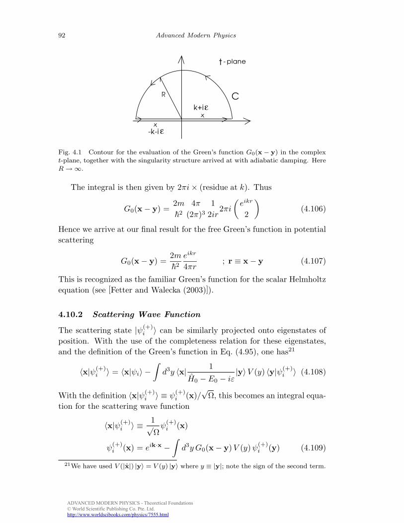
ADVANCED MODERN PHYSICS - Theoretical Foundations© World Scientific Publishing Co. Pte. Ltd.http://www.worldscibooks.com/physics/7555.html
J a n u a ry 27 , 2010 10:37 W S P C / B o o k T rim S iz e fo r 9 in x 6 in V 2ro o t
92 A d vanced M od ern P hysics
k+i
C
t
-k- i
R
- p la n e
F ig . 4 .1 C o n to u r fo r th e e v a lu a tio n o f th e G re e n ’s fu n c tio n G0(x − y) in th e c o m p le xt-p la n e , to g e th e r w ith th e sin g u la rity stru c tu re a rriv e d a t w ith a d ia b a tic d a m p in g . H e reR →∞.
T he integral is then given by 2πi× (residue at k). T hus
G0(x− y) =2m
~2
4π
(2π)31
2ir2πi
(
eik r
2
)
(4.10 6)
H ence we arrive at our fi nal result for the free G reen’s function in potential
scattering
G0(x− y) =2m
~2
eik r
4πr; r ≡ x− y (4.10 7 )
T his is recognized as the familiar G reen’s function for the scalar H elmholtz
eq uation (see [F etter and W aleck a (20 0 3 )]).
4 .1 0 .2 Scattering Wave Function
T he scattering state |ψ(+ )i 〉 can be similarly projected onto eigenstates of
position. W ith the use of the completeness relation for these eigenstates,
and the defi nition of the G reen’s function in E q . (4.95 ), one has21
〈x|ψ(+ )i 〉 = 〈x|ψi〉 −
∫
d3y 〈x| 1
H0 − E0 − iε|y〉V (y) 〈y|ψ(+ )
i 〉 (4.10 8 )
W ith the defi nition 〈x|ψ(+ )i 〉 ≡ ψ
(+ )i (x)/
√Ω, this becomes an integral eq ua-
tion for the scattering wave function
〈x|ψ(+ )i 〉 ≡ 1√
Ωψ
(+ )i (x)
ψ(+ )i (x) = eik·x −
∫
d3y G0(x− y)V (y)ψ(+ )i (y) (4.10 9)
21 W e h a v e u se d V (|x|) |y〉 = V (y) |y〉 w h e re y ≡ |y|; n o te th e sig n o f th e se c o n d te rm .

ADVANCED MODERN PHYSICS - Theoretical Foundations© World Scientific Publishing Co. Pte. Ltd.http://www.worldscibooks.com/physics/7555.html
J a n u a ry 27 , 2010 10:37 W S P C / B o o k T rim S iz e fo r 9 in x 6 in V 2ro o t
Scattering Theory 93
4 .1 0 .3 T -m atrix
T he T -matrix can also be expressed in the coordinate representation as
Tfi =
∫
d3y 〈kf |y〉V (y) 〈y|ψ(+ )i 〉 (4.110 )
where the fi nal state is now written explicitly as an eigenstate of momentum
|ψf 〉 ≡ |kf 〉. W ith the introduction of the corresponding wave functions,
one has
Tfi =1
Ω
∫
d3y e−ikf ·y V (y)ψ(+ )i (y) (4.111)
4 .1 0 .4 C ross Section
T he diff erential cross section follows from the transition rate according to
E q . (4.45 )
dσ =2π
~δ(Ef − E0)|Tfi|2
dn f
Iin c(4.112)
In this expression:
(1) T he incident wave function is ψi(x) = eik·x/√
Ω. T his yields an inci-
dent probability fl ux of
Iin c =1
Ω
~k
m(4.113 )
(2) T he number of fi nal states in a big box with periodic boundary condi-
tions is
dn f =Ω
(2π)3d3kf =
Ω
(2π)3k2
fdkf dΩf (4.114)
(3 ) T he integral over the energy-conserving delta function gives∫
δ(Ef − E0)k2fdkf =
2m
~2
kf
2; |kf | = |k| (4.115 )
(4) A combination of the results in E q s. (4.112)– (4.115 ) gives
dσ
dΩf=
2π
~
[
Ω
(2π)3mk
~2
] [
Ωm
~k
]
|Tfi|2 (4.116)
T he factors of Ω cancel, as they must, and the fi nal result for the
diff erential cross section for elastic scattering of a particle of energy

ADVANCED MODERN PHYSICS - Theoretical Foundations© World Scientific Publishing Co. Pte. Ltd.http://www.worldscibooks.com/physics/7555.html
J a n u a ry 27 , 2010 10:37 W S P C / B o o k T rim S iz e fo r 9 in x 6 in V 2ro o t
94 A d vanced M od ern P hysics
E0 = ~2k2/2m from the potential V (|x|) tak es the form
dσ
dΩf= |f(k,θ)|2
f(k,θ) ≡ − 1
4π
2m
~2
∫
d3y e−ikf ·y V (y)ψ(+ )i (y) (4.117 )
T he minus sign is conventional.
(5 ) T he scattering wave function ψ(+ )i (x) in this expression is the solution
to the integral eq uation
ψ(+ )i (x) = eik·x − 2m
~2
∫
d3yeik |x−y|
4π|x− y| V (y)ψ(+ )i (y) (4.118 )
4 .1 0 .5 U nitarity
T he scattering amplitude f(k,θ) and the T -matrix are related through
E q s. (4.117 ) and (4.111), and thus
− 2
~Im Tii =
4π
Ω
~
mIm f(k, 0 ) (4.119)
T he unitarity relation in E q . (4.94) states that
− 2
~Im Tii =
∑
f
2π
~δ(Ef − E0)|Tfi|2 (4.120 )
W ithin a factor of the incident fl ux, the r.h.s. of this relation is just the
total cross section σto t. T hus E q . (4.120 ) can be rewritten as
− 2
~Im Tii = Iin c σto t =
1
Ω
~k
mσto t (4.121)
A comparison of E q s. (4.119) and (4.121) then leads to the op tical th eorem
relating the imaginary part of the forward elastic scattering amplitude and
the total cross section22
Im f(k, 0 ) =k
4πσto t ; optical theorem (4.122)
T he analysis of potential scattering in this section provides the under-
lying basis for the study of scattering in q uantum mechanics, as presented,
for example, in [S chiff (1968 )].23
22S o fa r, th e re is o n ly e la stic sc a tte rin g in th is p o te n tia l m o d e l, b u t th e o p tic a l th e o re mis m o re g e n e ra l a n d h o ld s in th e p re se n c e o f a d d itio n a l in e la stic p ro c e sse s.
23 P ro b le m s 1.1– 1.5 in [W a le ck a (2 0 0 4 )] ta k e th e re a d e r th ro u g h th e e sse n tia ls o f th ep a rtia l-w a v e a n a ly sis o f th e sc a tte rin g p ro b le m .


![arXiv:0711.3941v2 [cs.CR] 27 Sep 2008brusso/endnote7CH5braidcrypt75pp.pdf · arXiv:0711.3941v2 [cs.CR] 27 Sep 2008 April 16, 2009 22:45 World Scientific Review Volume - 9in x 6in](https://img.dokumen.tips/doc/110x75/5fa837a90c439a24097719c6/arxiv07113941v2-cscr-27-sep-2008-brussoendno-arxiv07113941v2-cscr.jpg)