Advanced Microeconomics II

by Jinwoo Kim

November 24, 2010

Contents

II Mechanism Design 3

1 Preliminaries 3

2 Dominant Strategy Implementation 5

2.1 Gibbard-Satterthwaite Theorem . . . . . . . . . . . . . . . . . . . . . . . . 6

2.2 Dominant Strategy Implementation in Quasilinear Environment . . . . . . 9

2.3 Appendix: Envelope Theorem . . . . . . . . . . . . . . . . . . . . . . . . . 13

3 Nash and Subgame Perfect Implementation 15

3.1 Nash Implementation . . . . . . . . . . . . . . . . . . . . . . . . . . . . . . 15

3.2 Subgame Perfect Implementation . . . . . . . . . . . . . . . . . . . . . . . 17

4 Bayesian Implementation 21

4.1 General Results in Quasilinear Environment . . . . . . . . . . . . . . . . . 22

4.2 Single-Unit Auctions . . . . . . . . . . . . . . . . . . . . . . . . . . . . . . 27

4.2.1 Second-Price Auctions and English Auctions. . . . . . . . . . . . . 27

4.2.2 First-Price Auctions . . . . . . . . . . . . . . . . . . . . . . . . . . 28

1

4.2.3 Revenue Equivalence and Optimal Auctions . . . . . . . . . . . . . 30

4.2.4 Optimal Auction with Correlated Values . . . . . . . . . . . . . . . 32

4.3 Bilateral Trade . . . . . . . . . . . . . . . . . . . . . . . . . . . . . . . . . 34

4.3.1 Impossibility Result . . . . . . . . . . . . . . . . . . . . . . . . . . . 34

4.3.2 Double Auction . . . . . . . . . . . . . . . . . . . . . . . . . . . . . 35

4.4 Dissolving Partnerships Efficiently . . . . . . . . . . . . . . . . . . . . . . . 37

5 Principal-Agent Problem: Screening 39

6 Principal-Agent Problem: Moral Hazard 42

2

Part II

Mechanism Design

1 Preliminaries

So far, we have fixed an economic institution/mechanism, mostly at the competitive mar-ket, and investigated whether its equilibrium gives us an efficient outcome under variouscircumstances. The mechanism design theory reverses this procedure, that is we here fixsome social outcome we want to achieve, and ask what mechanism can implement suchoutcome for us.

• Let X denote the set of all social alternatives.

– As before, R : Set of all possible preferences over X; P : Set of all strict prefer-ences.

– Ri : Set of agent i’s possible preferences.

– Θi : Agent i’s type space. Θ ≡ Θ1 × · · · ×ΘI .

– For each type θi ∈ Θi, there is a corresponding preference in Ri, denoted %i (θi),which is represented by a utility function ui(·, θi).

• Let f : Θ � X denote the social choice rule (or correspondence), meaning that giventype profile θ ∈ Θ, f(θ) ⊂ X is the set of alternatives we want to achieve. Theexamples are:

1. fPE(θ) = {x ∈ X : There is no y ∈ X such that ui(y, θi) ≥ ui(x, θi),∀i with atleast one strict inequality} , that is fPE(θ) is the set of PE alternatives.

2. fMaj(θ) = {x : #{i : ui(x, θi) ≥ ui(y, θi)} ≥ I2, ∀y ∈ X}, that is fMaj(θ) is the

set of Condorcet winners in the pairwise majority voting.

3. fUtil(θ) = {x : x ∈ argmaxy∈X∑

i∈I ui(y, θi)}, that is fUtil(θ) is the set ofutilitarian welfare maximizers.

3

• If f(·) is single-valued (or f(θ) is a singleton set for all θ), then it is called socialchoice function (SCF).

Definition 1.1. f(·) is ex-post efficient (or Paretian) if for any θ ∈ Θ, we have f(θ) ⊂fPE(θ).

• A mechanism Γ = (S1, · · · , SI , g(·)) is a collection of strategy sets S1, · · · , SI andoutcome function g : S1 × · · · × SI → X.

– Let si(θi) ∈ Si denote the strategy played by agent i of type θi and s(θ) =

(s1(θ1), · · · , sI(θI))

– Let Eq(θ) ≡ {x ∈ X : x = g(s(θ)), where s(θ) is an equilibrium given θ}, thatis the set of all equilibrium outcomes given type profile θ.

Definition 1.2. A mechanism Γ implements a social choice rule f(·) if for every θ ∈ Θ,

there exists an equilibrium s(θ) such that g(s(θ)) ∈ f(θ).

Note: This concept of implementation is relatively weak in the following senses: (i) It onlyrequires that some, not all, alternative belonging to f(θ) can be achieved as an equilibriumoutcome; (ii) It does not rule out the possibility of equilibrium whose outcome lies outsidef(θ) (so some unwanted outcome might arise in some equilibrium).

Definition 1.3. A mechanism Γ fully implements a social choice rule f(·) if for everyθ ∈ Θ, there exists Eq(θ) = f(θ).

• Suppose that f(·) is single-valued or SCF. Then, a direct revelation mechanism(DRM) is a mechanism in which Si = Θi for all i ∈ I and g(θ) = f(θ) for allθ ∈ Θ.

– An interpretation of DRM is that each agent is asked to report his/her type and,given the reported type profile, the outcome is chosen following the SCF f(·).

– An SCF f(·) is truthfully implementable if the truth-telling is an equilibrium ofthe DRM.

Depending on the equilibrium concept we use, there are many notions of implementationavailable. Among others, we will see the implementation in dominant strategy, Nash, andBayesian Nash equilibrium in this order.

4

2 Dominant Strategy Implementation

• Given a mechanism Γ, s∗(θ) = (s∗1(θ1), · · · , s∗I(θI)) is a (weak) dominant strategy(DS) equilibrium in state θ if for all i,

ui(g(s∗i (θi), s−i), θi) ≥ ui(g(si, s−i), θi), ∀si ∈ Si,∀s−i ∈ S−i. (1)

– As well known, the advantage of dominant strategy equilibrium is that agentsdo not need to know about other agents’ information/strategy.

– If agents have strict preference, then the DS outcome must be unique for anyprofile θ.

Proof. Consider any two DS equilibria s∗ and s∗∗ given type profile θ. Since s∗1and s∗∗1 are both dominant for agent 1, he must be indifferent between g(s∗1, s∗−1)

and g(s∗∗1 , s∗−1) so g(s∗1, s

∗−1) = g(s∗∗1 , s

∗−1) (since the preference is strict). For

the same reason, agent 2 must be indifferent be between g(s∗∗1 , s∗2, s

∗−{1,2}) and

g(s∗∗1 , s∗∗2 , s

∗−{1,2}) so g(s∗∗1 , s

∗2, s

∗−{1,2}) = g(s∗∗1 , s

∗∗2 , s

∗−{1,2}). Repeating this way,

we obtain

g(s∗) = g(s∗∗1 , s∗−1) = g(s∗∗1 , s

∗∗2 , s

∗−{1,2}) = · · · = g(s∗∗),

as desired.

Definition 2.1. The mechanism Γ implements the social choice rule f in DS if for everyθ ∈ Θ, there exists a DS equilibrium s∗(θ) such that g(s∗(θ)) ∈ f(θ).

• An SCF f(·) is truthfully implementable in DS if s∗i (θi) = θi (or truth-telling) is a DSequilibrium for all θi ∈ Θi and all i ∈ I, that is

ui(f(θi,θ−i), θi) ≥ ui(f(θ′i, θ−i), θi),∀θ′i, ∀θ−i. (2)

The revelation principle below greatly simplifies our analysis since it allows us to restrictour attention to DRM rather the entire set of possible mechanisms.

Proposition 2.2 (Revelation Principle for DS Implementation). Suppose that there existsa mechanism Γ that implements the SCF f(·) in DS. Then, f(·) is truthfully implementablein DS.

5

Proof. If Γ implements f(·) in DS, then there exists s∗(·) = (s∗1(·), · · · , s∗I(·)) satisfying (1),which implies

ui(g(s∗i (θi), s

∗−i(θ−i)), θi) ≥ ui(g(s

∗i (θ

′i), s

∗−i(θ−i)), θi),∀θ′i,∀θ−i.

Thus, since g(s∗(·)) = f(·), we have

ui(f(θi,θ−i), θi) ≥ ui(f(θ′i, θ−i), θi),∀θ′i,∀θ−i,

which is precisely the condition (2).

2.1 Gibbard-Satterthwaite Theorem

From now, we will explore the implication of DS implementation toward proving Gibbard-Satterthwaite theorem, which says that only dictatorial social choice functions are imple-mentable in DS.

• Define the lower contour set of alternative x when agent i has type θi as:

Li(s, θi) = {y ∈ X : ui(x, θi) ≥ ui(y, θi)}.

Then, the following is immediate.

Lemma 2.3 (Preference Reversal). The SCF f(·) is truthfully implementable in DS if andonly if for all i ∈ I, all θ−i ∈ Θ−i and for all pairs of types θi, θ′i ∈ Θi, we have

f(θ′i, θ−i) ∈ Li(f(θi, θ−i), θi) and f(θi, θ−i) ∈ Li(f(θ′i, θ−i), θ

′i).

6

Definition 2.4. The SCF f(·) is dictatorial if there is an agent i such that for all θ ∈ Θ,

f(θ) ∈ {x ∈ X : ui(x, θi) ≥ ui(y, θi),∀y ∈ X},

that is f(·) always chooses one of i’s top-ranked alternatives.

Definition 2.5. The SCF f(·) is monotonic if the following holds for any θ : If θ′ is suchthat Li(f(θ), θi) ⊂ Li(f(θ), θ

′i), ∀i ∈ I, then f(θ′) = f(θ).

Lemma 2.6. If Ri = P ,∀i ∈ I, and f(·) is truthfully implementable in DS, then f(·) ismonotonic.Note: It follows from the assumption Ri = P, ∀i that f(·) is single-valued or an SCF.

Proof. Consider two profiles θ and θ′ such that Li(f(θ), θi) ⊂ Li(f(θ), θ′i),∀i. Let’s show

that f(θ′) = f(θ). Consider two profiles (θ1,θ−1) and (θ′1, θ−1). The truth-telling beingdominant for agent 1 implies

f(θ′1, θ−1) ∈ L1(f(θ), θ1) ⊂ L1(f(θ), θ′1) and f(θ) ∈ L1(f(θ

′1, θ−1), θ

′1).

Since agent 1’s preference (under θ′1) is strict, this implies f(θ′1, θ−1) = f(θ). The same rea-soning can be applied to profiles (θ′1, θ2, θ−{1,2}) and (θ′1, θ

′2, θ−{1,2}), which yields f(θ′1, θ′2, θ−{1,2}) =

f(θ′1, θ−1). Repeating in this fashion, we obtain

f(θ) = f(θ′1, θ−1) = f(θ′1, θ′2, θ−{1,2}) = · · · = f(θ′),

as desired.

Theorem 2.7 (Gibbard-Satterthwaite Theorem). Suppose that

(i) X is finite and |X| ≥ 3,

(ii) Ri = P, ∀i ∈ I,

(iii) for all x ∈ X, there exists θ ∈ Θ such that x = f(θ).

Then, the SCF f(·) is implementable in DS if and only if it is dictatorial.

Proof. It is immediate that f(·) is truthfully implementable if it is dictatorial. So we focuson showing the converse. Throughout the proof, given any type θi of agent i and anysubset A ⊂ X of alternatives, we will let θAi denote another type whose preference ranks

7

the alternatives in A most highly while keeping all other rankings the same as in θ. Theproof is done in a few steps.

Step 1 : f(·) is ex post efficient.

Proof. Suppose not. Then there is θ ∈ Θ and x ∈ X such that ui(x, θi) > ui(f(θ), θi),∀i(since the preferences are strict by (ii)). Also, by (iii), there is θ ∈ Θ such that x = f(θ).

Then, consider a profile ˆθ in which ˆ

θi = θ{x,f(θ)}i for each i ∈ I. Note that x is top-ranked

according to ˆθi for all i since it is preferred to f(θ). Thus,

Li(x, θi) ⊂ Li(x,ˆθi) and Li(f(θ), θi) ⊂ Li(f(θ),

ˆθi),∀i. ∈ I.

Then, the monotonicity of f(·) implies f(ˆθ) = f(θ) = x and also f(ˆθ) = f(θ), a contradic-tion because x = f(θ).

Before proceeding, let us define a social welfare function F : Θ → R as follows: For anypair x, y ∈ X and profile θ ∈ Θ,

xFp(θ)y if and only if x = f(θ{x,y}).

We verify that the social welfare function defined above satisfies all conditions of Arrow’simpossibility theorem. It is clear that F (·) is weakly Paretian since f(·) is ex post efficient.

Step 2 : F (·) satisfies IIA property.

Proof. Consider two alternative x, y ∈ X and two profiles θ, θ ∈ Θ such that the rankingbetween x and y is the same across θi and θi for all i, which implies that

Li(x, θ{x,y}i ) = Li(x, θ

{x,y}i ) and Li(y, θ

{x,y}i ) = Li(y, θ

{x,y}i ),∀i ∈ I. (3)

Suppose now that xFp(θ)y or f(θ{x,y}) = x. Since f(·) is monotonic, due to (3), we musthave f(θ{x,y}) = x so xFp(θ)y. Also, for the same reasoning, if yFp(θ)x, then we must havef(θ{x,y}) = y so yFp(θ)x.

It remain to show that F (θ) for any θ is indeed a preference, for which it suffices toprove the transitivity of F (θ).

Step 3 : For any profile θ ∈ Θ, F (θ) is transitive.

8

Proof. Consider three alternatives x, y, z satisfying xFp(θ)y and yFp(θ)z. We first showthat f(θ{x,y,z}) = x. For this, note that

Li(y, θ{x,y,z}i ) ⊂ Li(y, θ

{x,y}i ) and Li(z, θ

{x,y,z}i ) ⊂ Li(z, θ

{y,z}i ),∀i ∈ I,

which implies that by the monotonicity of f(·), if f(θ{x,y,z}) = y, then f(θ{x,y}) = y,contradicting xFp(θ)y while if f(θ{x,y,z}) = z, then f(θ{y,z}) = z, contradicting yFp(θ)z.

Given this and the ex-post efficiency of f(·), we must have f(θ{x,y,z}) = x. Also, since

Li(x, θ{x,y,z}i ) ⊂ Li(x, θ

{x,z}i ), ∀i ∈ I,

we must have f(θ{x,z}) = x by the monotonicity of f(·), meaning that xFp(θ)z, as desired.

Thus, by the Arrow’s theorem, we conclude that F (·) is dictatorial, that is there is someagent h such that for any θ ∈ Θ

xFp(θ)y ⇐⇒ x ≻h (θh)y. (4)

Using this, we now show that f(·) is also dictatorial. For this, consider any profile θ and anyalternative x = f(θ). Then, by the monotonicity, we have f(θ{x,f(θ)}) = f(θ) or f(θ)Fp(θ)x,

which implies f(θ) ≻h (θh)x due to (4).

2.2 Dominant Strategy Implementation in Quasilinear Environ-

ment

• Let us assume that the set of social alternatives is given as

X = {x = (k, t1, · · · , tI) : k ∈ K and ti ∈ R,∀i},

where k denotes a project choice and belongs to a (finite) set K while ti denotes thetransfer to agent i.

– Each agent i’s preference is given as

ui(x, θi) = vi(k, θi) + ti. (5)

9

– Let V denote the set of all possible functions v : K → R.

Example 2.8 (Single Item Auction). Suppose that there is one indivisible object to beallocated to one of I bidders. Then, k = (y1, · · · , yI), yi ∈ {0, 1},∀i and

∑yi ≤ 1. Letting

θi be the value attached to the object by bidder i, we have vi(k, θi) = θiyi. `

• Let k∗ : Θ → K be a function satisfying∑i∈I

vi(k∗(θ), θi) ≥

∑i∈I

vi(k, θi), ∀k ∈ K,

that is an efficient project choice rule.

Proposition 2.9. An SCF f(·) = (k∗(·), t1(·), · · · , tI(·)) is truthfully implementable in DSif

ti(θ) = tVi (θ) ≡∑j =i

vj(k∗(θ), θj) + hi(θ−i), ∀i ∈ I,∀θ ∈ Θ, (6)

where hi(·) is an arbitrary function of θ−i.

Proof. Suppose for a contradiction that there exist i, θi, θ′i and θ−i such that

vi(k∗(θ′i, θ−i), θi) + ti(θ

′i, θ−i) > vi(k

∗(θi, θ−i), θi) + ti(θi, θ−i).

With the substitution of (6), this implies∑j∈I

vj(k∗(θ′i, θ−i), θj) >

∑j∈I

vj(k∗(θi, θ−i), θj),

which contradicts with the definition of k∗.

Note: The DRM (k∗, tV1 , · · · , tVI ) is so called “Vickrey-Clark-Groves (VCG)” mechanism.

Proposition 2.10. Suppose that {vi(·, θ) : θi ∈ Θi} = V , ∀i. Then, an SCF f(·) =

(k∗(·), t1(·), · · · , tI(·)) is truthfully implementable in DS only if (6) holds.

Proof. One can write

ti(θi, θ−i) =∑j =i

vj(k∗(θi, θ−i), θj) + hi(θi, θ−i). (7)

10

We need to show that the function hi should not depend on θi in order for f(·) to betruthfully implementable in DS. Let us consider two type profiles (θi, θ−i) and (θ′i, θ−i).

If k∗(θi, θ−i) = k∗(θ′i, θ−i), then by (7), we must have hi(θi, θ−i) = hi(θ′i, θ−i) as de-

sired. So assume that k∗(θi, θ−i) = k∗(θ′i, θ−i). For convenience, denote k∗ ≡ k∗(θi, θ−i)

k′ ≡ k∗(θ′i, θ−i). Suppose for a contradiction that hi(θi, θ−i) > h(θ′i, θ−i). (The case wherehi(θi, θ−i) < h(θ′i, θ−i) can be dealt with analogously). We can find a type θϵi such that forsmall ϵ > 0,

vi(k, θϵi ) =

−∑

j =i vj(k∗, θj) if k = k∗

−∑

j =i vj(k′, θj) + ϵ if k = k′

−∞ otherwise

.

Thus, k∗(θϵi , θ−i) = k′ and hi(θϵi , θ−i) = hi(θ′i, θ−i). Also, we must have

vi(k′, θϵi ) + ti(θ

ϵi , θ−i) ≥ vi(k

∗, θϵi ) + ti(θi, θ−i),

which implies ϵ + hi(θϵi , θ−i) ≥ hi(θi, θ−i). Since ϵ can be arbitrarily small, this means

hi(θ′i, θ−i) = hi(θ

ϵi , θ−i) ≥ hi(θi, θ−i), a contradiction.

• Among many VCG mechanisms, the pivotal mechanism is defined as

tPi (θ) ≡

[∑j =i

vj(k∗(θ), θj)

]−

[∑j =i

vj(k∗−i(θ−i), θj)

], (8)

wherek∗−i(θ−i) ∈ argmax

k∈K

∑j =i

vj(k, θj).

– Apply (8) to the auction environment to obtain

tPi (θ) =

−maxj =i θj if θi > maxj =i θj

0 otherwise,

which corresponds to the second-price auction that makes the bidder with thehighest valuation pay the second highest valuation.

• We say that an SCF (k(·), t1(·), · · · , tI(·)) is (ex-post) budget-balanced if∑i∈I

ti(θ) = 0, ∀θ ∈ Θ.

11

– Sometimes ex-post budget-balancing is considered as part of ex-post efficiencysince it requires none of the numeraire should be wasted.

– As a weaker notion of budget balancedness, the SCF is is said to be ex-antebudget balanced if

E

[∑i∈I

ti(θ)

]= 0.

– We say that the SCF satisfies no ex-ante budget deficit if

E

[∑i∈I

ti(θ)

]≤ 0.

Proposition 2.11. Suppose that K = {0, 1} and {vi(·, θ) : θi ∈ Θi} = V ,∀i. Then,there is no SCF f(·) = (k∗(·), t1(·), · · · , tI(·)) that is truthfully implementable in DS andbudget-balanced.

Proof. Suppose, to the contrary, that such a mechanism exists. Without loss of generality,we can normalize vi(0, θi) = 0,∀θi, ∀i. Pick θ1, θ1, and θ2 such that

v1(1, θ1) + v2(1, θ2) > 0 and v1(1, θ1) + v2(1, θ2) < 0. (9)

Then, by applying Proposition 2.10, we have that

v1(1, θ1) + v2(1, θ2) + h1(θ2) + h2(θ1) =∑i=1,2

ti(θ1, θ2) = 0

h1(θ2) + h2(θ1) =∑i=1,2

ti(θ1, θ2) = 0,

which can be subtracted side-by-side to yield

v1(1, θ1) + h2(θ1)− h2(θ1) = −v2(1, θ2).

Here the left-hand side is independent of θ2 while the right-hand side is not. So this equalitycannot hold with the varying values of θ2 within the set satisfying (9). For the case of I ≥ 3,refer to Green and Laffont (1979).

12

The Differentiable Case

Assumption D. For all i ∈ I, Θi = [¯θi, θi], and vi(k, θi) is a C1 function for all k ∈ K.

Given this assumption, we obtain a chacracterization of DS implementability similar to theProposition 2.10:

Theorem 2.12. Under Assumption D, an SCF f(·) = (k∗(·), t1(·), · · · , tI(·)) is truthfullyimplementable in DS only if (6) holds.

Proof. Note first that the VCG mechanism f(·) = (k∗(·), tV1 (·), · · · , tVI (·)) defined in (6)is truthfully implementable in DS. Now consider any DS implementable SCF f(·) =

(k∗(·), t1(·), · · · , tI(·)) and then we must have that for any given θ−i,

θi ∈ argmaxθ′i

vi(k∗(θ′i, θ−i), θi) + ti(θ

′i, θ−i),

which implies by the envelope theorem (in the Appendix of this Section) that

vi(k∗(θ), θi) + ti(θ) = vi(k

∗(¯θi, θ−i),

¯θi) + ti(

¯θi, θ−i) +

∫ θi

¯θi

∂vi(k∗(s, θ−i), s)

∂θids

orti(θ) = vi(k

∗(¯θi, θ−i),

¯θi) + ti(

¯θi, θ−i) +

∫ θi

¯θi

∂vi(k∗(s, θ−i), s)

∂θids− vi(k

∗(θ), θi).

Since this holds true for any DS implementable SCF and the VCG mechanism is DS im-plementable,

ti(θ)− tVi (θ) = ti(¯θi, θ−i)− tVi (¯

θi, θ−i),

from which the desired conclusion follows because ti(¯θi, θ−i)− tVi (¯

θi, θ−i) is independent ofθi.

Green and Laffont (1977) shows that an impossibility result similar to the Proposition2.11 obtains in the differentiable case also.

2.3 Appendix: Envelope Theorem

The envelope theorem gives us a formula about how the value of a parameterized optimiza-tion problem responds to the marginal change in the parameter.

13

• Letting X be the choice set, t ∈ [0, 1] the relevant parameter, and f : X × [0, 1] → R,let us define

V (t) = supx∈X

f(x, t)

X∗(t) = {x ∈ X : f(x, t) = V (t)}.

Theorem (Milgrom and Segal). Suppose that f(x, ·) is absolutely continuous for all x ∈ X.

Suppose also that there exists an integrable function b : [0, 1] → R+such that |ft(x, t)| ≤ b(t)

for all x ∈ X and almost all t ∈ [0, 1].Then V is absolutely continuous. Suppose, in addition,that f(x, ·) is differentiable for all x ∈ X, and X∗(t) = ∅ almost everywhere on [0, 1]. Then,for any selection x∗(t) ∈ X∗(t),

V (t) = V (0) +

∫ t

0

ft(x∗(s), s)ds.

14

3 Nash and Subgame Perfect Implementation

We have seen that not many SCF’s can be implemented via dominant strategy equilibrium.This is related to the fact that only few games admit a dominant strategy equilibrium. Sorequiring a weaker equilibrium concept, whose existence is guaranteed in most circum-stances, is one way to fix the problem. In this section, we explore how a weaker equilibriumconcept, such as Nash or subgame perfect equilibrium, can expand the set of implementableoutcomes.

3.1 Nash Implementation

In many circumstances, agents share a great deal of knowledge among themselves whilean outsider (or mechanism designer) does not. It is interesting to know how a mechanismdesigner can utilize such knowledge to achieve the desired outcome. Thus we here assumethat all agents are informed of θ = (θ1, · · · , θI) ∈ Θ while the designer is uninformed, whichis so called complete information environment. The right concept of equilibirium in thissetup is Nash equilibrium (NE) so we define:

Definition 3.1. A mechanism Γ = (S1, · · · , SI , g) (fully or strongly) implements an SCFf in Nash equilibrium if for each θ ∈ Θ, (i) there exists a Nash equilibrium s∗(θ) =

(s∗1(θ), · · · , s∗I(θ)) such that g(s∗(θ)) = f(θ) and (ii) every Nash equilibrium results inoutcome f(θ).

A crucial condition for the Nash implementation is the monotonicity defined in theDefinition 2.5.

Theorem 3.2. If f is implementable in Nash equilibrium, then it is monotonic.

Proof. Suppose that f is not monotonic. Then, there exists θ and θ′ such that Li(f(θ), θi) ⊂Li(f(θ), θ

′i), ∀i but f(θ′) = f(θ). Consider a NE s∗(θ) with g(s∗(θ)) = f(θ) and then it is

also Nash equilibrium in state θ′ since

g(si, s∗−i(θ−i)) ∈ Li(g(s

∗(θ)), θi) ⊂ Li(g(s∗(θ)), θi),∀si ∈ Si, ∀i,

which contradicts with f being implementable in NE.

15

The monotonicity is also sufficient for the NE impelementability when coupled with anadditional property called “no veto power”

Definition 3.3. f satisfies no veto power (NVP) if no agent i has a veto power in thesense that if there exists some x ∈ X such that

uj(x, θj) ≥ uj(y, θj),∀y ∈ X, ∀j = i,

then f(θ) = x.

Theorem 3.4. If I ≥ 3 and f is monotonic and satisfies NVP, then f is implementablein NE.

Proof. We aim to construct a mechanism that implements f in NE. Let Si = Θ × X ×{0, 1, 2, 3, · · · } and si = (θi, xi,mi) ∈ Si, where θi = (θi1, · · · , θiI) is a preference profile(preferences of all agents) reported by i, xi is an alternative, and mi is a number that ichooses. Then a mechanism Γ = (S1, · · · , SI , g) is defined as follows:

Case I: If for all i ∈ I, (θi, xi) = (θ, x) for some (θ, x) satisfying x = f(θ), then g(s1, · · · , sI) =f(θ).

Case II: If for all j = i, (θj, xj) = (θ, x) for some (θ, x) satisfying x = f(θ), then

g(s1, · · · , sI) =

xi if ui(x, θi) ≥ ui(xi, θi)

x otherwise.(10)

Case III: For all other strategies, let g(s1, · · · , sI) = xi, where i = argmaxi∈I mi.

The proof that Γ implements f in NE consists of 4 steps.

Step 1 : If (θi, xi) = (θ, x),∀i satisfying x = f(θ), then (s1, · · · , sI) forms a NE in θ andg(s1, · · · , sI) = x.

Proof. If agent i deviates to report some (θ′, x′) = (θ, x), then x′ is chosen over x only whenthe first condition of (10) holds, so the deviation is unprofitable.

Step 2 : If (θixi) = (θ, x),∀i satisfying x = f(θ), and (s1, · · · , sI) is a NE in θ, then x = f(θ).

16

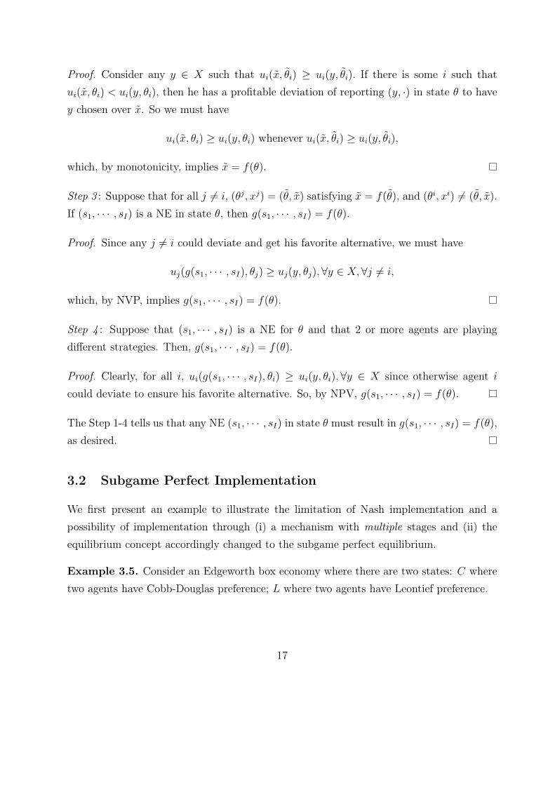
Proof. Consider any y ∈ X such that ui(x, θi) ≥ ui(y, θi). If there is some i such thatui(x, θi) < ui(y, θi), then he has a profitable deviation of reporting (y, ·) in state θ to havey chosen over x. So we must have

ui(x, θi) ≥ ui(y, θi) whenever ui(x, θi) ≥ ui(y, θi),

which, by monotonicity, implies x = f(θ).

Step 3 : Suppose that for all j = i, (θj, xj) = (θ, x) satisfying x = f(θ), and (θi, xi) = (θ, x).

If (s1, · · · , sI) is a NE in state θ, then g(s1, · · · , sI) = f(θ).

Proof. Since any j = i could deviate and get his favorite alternative, we must have

uj(g(s1, · · · , sI), θj) ≥ uj(y, θj),∀y ∈ X, ∀j = i,

which, by NVP, implies g(s1, · · · , sI) = f(θ).

Step 4 : Suppose that (s1, · · · , sI) is a NE for θ and that 2 or more agents are playingdifferent strategies. Then, g(s1, · · · , sI) = f(θ).

Proof. Clearly, for all i, ui(g(s1, · · · , sI), θi) ≥ ui(y, θi),∀y ∈ X since otherwise agent icould deviate to ensure his favorite alternative. So, by NPV, g(s1, · · · , sI) = f(θ).

The Step 1-4 tells us that any NE (s1, · · · , sI) in state θ must result in g(s1, · · · , sI) = f(θ),

as desired.

3.2 Subgame Perfect Implementation

We first present an example to illustrate the limitation of Nash implementation and apossibility of implementation through (i) a mechanism with multiple stages and (ii) theequilibrium concept accordingly changed to the subgame perfect equilibrium.

Example 3.5. Consider an Edgeworth box economy where there are two states: C wheretwo agents have Cobb-Douglas preference; L where two agents have Leontief preference.

17

.

.f(L)

.y

.x

.f(C)

Here f violates the monotonicity and thus cannot be implemented in NE. Nontheless, fcan be implemented as the unique subgame perfect equilibrium outcome of the followingthree-stage mechanism.

..A1

.f(L).Announce L

.A2

.f(C).Agree

.A1

.y.Choose y

.x.Choose x

.Challenge

.Announce C

State C : At the last stage, agent 1 should choose x over y. Anticipating this, agent 2should agree at the second stage. Then, the optimal reponse of agent 1 is to announce Cat the first stage.

18

State L : Agent 1 should choose y over x if the last stage were reached. Given this, agent 2should get y chosen by challenging at the stage 2 if agent 1 announces C at the first stage.So, agent 1 should announce L at the first stage in order to avoid y getting chosen.

Moore and Repullo (1988) (partially) characterize the set of SCF’s that are imple-mentable in SPE in general environment. In particular, almost any SCF can be imple-mented in SPE in economic environments where there is at least one private good.

Quasi-linear Environment Let us focus on the environment in which agents have quasi-linear preferences. In this environment also, many desirable SCF’s fail to be monotonicand thus are not implementable in NE. For instance, assume two agents and define f(·) =(k(·), t1(·), t2(·)) such that

k(θ) ∈ argmaxk∈K

∑i=1,2

vi(k, θi) and

ti(θi, θ−i) < ti(θ′i, θ−i) if vi(k, θi) > vi(k, θ

′i),∀k. (11)

Applied to the public good problem, (11) requires an agent to contribute more if he has ahigher WTP for public goods. This SCF is not implementable in NE. To see it, given anytype profile θ = (θ1, θ2), consider another profile θ′ = (θ′1, θ2) satisfying

v1(k, θ′1) = v1(k, θ1) + C, ∀k ∈ K, for some constant C > 0.

The monotonicity requires f(θ′) = f(θ), which contradicts with (11). Using the subgameperfect implementation, however, virtually all SCF’s are implementable in the quali-linearenvironment:

Theorem 3.6. Suppose that there are two agents and consider an SCF f(·) = (k(·), t1(·), t2(·))such that the utility of each agent i from f(·) is uniformly bounded, that is,

supθ∈Θ

vi(k(θ), θi) + ti(θ) < M for some M. (12)

Then, f is implementable in SPE.

Proof. We construct the following multi-stage game.

Stage 1 (eliciting agent 1’s preference):

19

..A1 .A2

.Go to Stage 2,.Agree

.A1

.(y, ty −∆t,−ty +∆t).Choose k = y and

.t1 = ty −∆t

.(x, tx −∆t,−tx −∆t).Choose k = x and

.t1 = tx −∆t

.announce ϕ1 = θ1

.Challenge and

.Announce θ1

where ∆t is a large positive number, and1

v1(x, θ1) + tx > v1(y, θ1) + ty and (13)

v1(x, ϕ1) + tx < v1(y, ϕ1) + ty; (14)

Stage 2 (eliciting agent 2’s preference): Same as Stage 1, except that the roles of agents1 and 2 are switched;

If both agents agree on θ = (θ1, θ2), then implement (k(θ), t1(θ), t2(θ)).

It is straightforward to argue that each agent has an incentive to tell the truth. Forinstance, if agent 1 lies, then agent 2 can challenge him with the truth ϕ1 = θ1, whereafteragent 1 will optimally choose (y, ty −∆t) due to (14). This is worse for agent 1 than tellingthe truth while it is better for agent 2 than agreeing, if ∆t is set sufficiently large, giventhe assumption (12). On the other hand, if agent 1 tells the truth, then agent 2 will not(falsely) challenge, since agent would then choose (x, tx −∆t) due to (13), which yields alarge penalty ∆t for agent 2.

1Note that one can always find x, y, tx, and ty satisfying (13) and (14). Otherwise we must have

v1(x, θ1)− v1(y, θ1) = v1(x, ϕ1)− v1(y, ϕ1), ∀x, y,

meaning that two types θ1 and ϕ1 have the same preference.

20

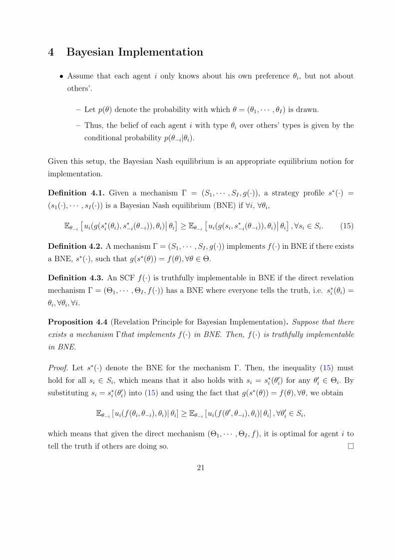
4 Bayesian Implementation

• Assume that each agent i only knows about his own preference θi, but not aboutothers’.

– Let p(θ) denote the probability with which θ = (θ1, · · · , θI) is drawn.

– Thus, the belief of each agent i with type θi over others’ types is given by theconditional probability p(θ−i|θi).

Given this setup, the Bayesian Nash equilibrium is an appropriate equilibrium notion forimplementation.

Definition 4.1. Given a mechanism Γ = (S1, · · · , SI , g(·)), a strategy profile s∗(·) =

(s1(·), · · · , sI(·)) is a Bayesian Nash equilibrium (BNE) if ∀i, ∀θi,

Eθ−i

[ui(g(s

∗i (θi), s

∗−i(θ−i)), θi)

∣∣ θi] ≥ Eθ−i

[ui(g(si, s

∗−i(θ−i)), θi)

∣∣ θi] , ∀si ∈ Si. (15)

Definition 4.2. A mechanism Γ = (S1, · · · , SI , g(·)) implements f(·) in BNE if there existsa BNE, s∗(·), such that g(s∗(θ)) = f(θ),∀θ ∈ Θ.

Definition 4.3. An SCF f(·) is truthfully implementable in BNE if the direct revelationmechanism Γ = (Θ1, · · · ,ΘI , f(·)) has a BNE where everyone tells the truth, i.e. s∗i (θi) =θi,∀θi,∀i.

Proposition 4.4 (Revelation Principle for Bayesian Implementation). Suppose that thereexists a mechanism Γthat implements f(·) in BNE. Then, f(·) is truthfully implementablein BNE.

Proof. Let s∗(·) denote the BNE for the mechanism Γ. Then, the inequality (15) musthold for all si ∈ Si, which means that it also holds with si = s∗i (θ

′i) for any θ′i ∈ Θi. By

substituting si = s∗i (θ′i) into (15) and using the fact that g(s∗(θ)) = f(θ),∀θ, we obtain

Eθ−i[ui(f(θi, θ−i), θi)| θi] ≥ Eθ−i

[ui(f(θ′, θ−i), θi)| θi] , ∀θ′i ∈ Si,

which means that given the direct mechanism (Θ1, · · · ,ΘI , f), it is optimal for agent i totell the truth if others are doing so.

21

Remark 4.5. Proposition 4.4 says that given any (possibly non-direct) mechanism Γ and itsBNE s∗, one can find a direct mechanism that implements the same outcome via a truthfulBNE. This means that whatever SCF we can implement, we must be able to implementit using a direct mechanism. In other words, if we cannot find any direct mechanism thatimplements a certain SCF, there is no, direct or indirect, mechanism that implements it.

4.1 General Results in Quasilinear Environment

Suppose that each agent i’s preference is given as in (5). We also assume that agents’types are independently distributed so for any function τ : Θ → R, Eθ−i

[τ(θi, θ−i)|θi] =Eθ−i

[τ(θi, θ−i)],∀θi.

AGV (d’Aspremont and Gerard-Varet) Mechanism Here we go back to the prob-lem of whether a mechanism can be both efficient and budget balanced. It is possibleto show that such mechanism does exist if the equilibrium concept is relaxed from thedominant strategy to the Bayesian Nash equilibrium. For doing so, define

ξi(θi) ≡ Eθ−i

[∑j =i

vj(k∗(θi, θ−i), θj)

],

that is the expected utility of other agents than i when the latter’s type is θi.

• AGV (direct) mechanism with SCF f(·) = (k∗(·), t(·)) is given as

ti(θ) = ξi(θi) + hi(θ−i),∀i,∀θ (16)

wherehi(θ−i) = −

(1

I − 1

)∑j =i

ξj(θj).

Proposition 4.6. AGV mechanism has the truth-telling as a BNE and is budget balanced.

Proof. To see the budget-balancedness, note∑i∈I

ti(θ) =∑i∈I

ξi(θi) +∑i∈I

hi(θ−i)

22

=∑i∈I

ξi(θi)−(

1

I − 1

)∑i∈I

∑j =i

ξj(θj)

=∑i∈I

ξi(θi)−(

1

I − 1

)∑i∈I

(I − 1)ξi(θi) = 0.

For the truth-telling part, note

Eθ−i[vi(k

∗(θi, θ−i), θi) + ti(θi, θ−i)]

=Eθ−i

[∑j∈I

vj(k∗(θi, θ−i), θj)

]+ Eθ−i

[hi(θ−i)]

≥Eθ−i

[∑j∈I

vj(k∗(θ′i, θ−i), θj)

]+ Eθ−i

[hi(θ−i)]

=Eθ−i[vi(k

∗(θ′i, θ−i), θi)) + ti(θ′i, θ−i)] ,

where the two equalities follow from (16) and the definition of ξi(·) while the inequalityfrom the efficiency of k∗(θ) when the type profile is θ.

Bayesian Implementation with Linear Utility

• Suppose now that the utility is linear in that given a social alternative x = (k, t),

ui(x, θi) = θivi(k) + ti.

– We also assume that each θi is distributed on Θi = [¯θi, θi] following a cdf Fi.

– Given a direct mechanism with SCF f(·) = (k(·), t(·)), let us define

vi(θi) ≡ Eθ−i[vi(k(θi, θ−i))]

ti(θi) ≡ Eθ−i[ti(k(θi, θ−i))] .

– If agent i of type θi announces θ′i, then his payoff is

Eθ−i[θivi(ki(θ

′i, θ−i)) + ti(θ

′i, θ−i)]

=θivi(θ′i) + ti(θ

′i).

– Let Ui(θi) ≡ θivi(θi) + ti(θi), that is agent i’s payoff in the truthful equilibriumof the direct mechanism with f(·) = (k(·), t1(·), · · · , tI(·)).

23

Example 4.7. In the auction environment of Example 2.8, vi(k) = yi and thus vi(θi) =Eθ−i

[yi(θi, θ−i)] is the expected winning probability for bidder i of type θi. `

Theorem 4.8. A direct mechanism (k(·), t(·)) is truthfully implementable in BNE if andonly if, for all i ∈ I and θi ∈ Θi,

(i) vi(·) is nondecreasing

(ii) For any given θ0i ∈ Θi,

Ui(θi) = Ui(θ0i ) +

∫ θi

θ0i

vi(s)ds,∀θi.

Proof. To prove the “only if” part, choose any θi and θ′i > θi. Since θi and θ′i (weakly)prefer telling the truth to reporting θ′i and θi, respectively, we have

Ui(θi) ≥ θivi(θ′i) + ti(θ

′i) = Ui(θ

′i) + (θi − θ′i)vi(θ

′i) (17)

Ui(θ′i) ≥ θ′ivi(θi) + ti(θi) = Ui(θi) + (θ′i − θi)vi(θi),

which can be rearranged to yield

vi(θ′i) ≥

Ui(θ′i)− Ui(θi)

θ′i − θi≥ vi(θi). (18)

So, vi(·) is nondecreasing. Also, as θ′i converges to θi, (18) yields U ′i(θi) = vi(θi),which

establishes (ii).

To prove the “if” part, let us consider any θi and show that θi (weakly) prefers tellingthe truth to reporting any other type θ′i < θi,

2 which will hold if (17) is satisfied. To seeit, use (ii) to derive

Ui(θi)− Ui(θ′i) =

∫ θi

θ′i

vi(s)ds

≥∫ θi

θ′i

vi(θ′i)ds

= (θi − θ′i)vi(θ′i),

where the inequality holds due to (i).2The argument for the case θ′i > θi is analogous.

24

Proposition 4.9. Consider any two mechanisms, Γ = (k, t) and Γ′ = (k, t′) that aretruthfully implementable in BNE, and their equilibrium payoffs Ui(·) and U ′

i(·). Then,there exists some constant ci for each i such that

Ui(θi) = U ′i(θi) + ci,∀θi.

Proof. From the Proposition 4.8, we must have

Ui(θi) = Ui(¯θi) +

∫ θi

¯θi

vi(s)ds

U ′i(θi) = U ′

i(¯θi) +

∫ θi

¯θi

vi(s)ds.

Letting ci ≡ Ui(¯θi)− U ′

i(¯θi), we obtain the desired result.

We now introduce the reservation utility, or the utility that an agent can obtain outsidethe mechanism.

• Letting Ui(θi) denote the reservation utility for θi, we call a mechanism (k, t) individ-ual rational if

Ui(θi) = θivi(θi) + ti(θi) ≥ U i(θi),∀θi, ∀i, (19)

that is each type θi is weakly better off participating in the mechanism.

So the set of inequalities (19) is also referred to as the participation constraint.

Fixing an efficient allocation rule at the efficient rule k∗, one can ask if there existsa mechanism (k∗, t) that is truthfully implementable while being individual rational andsatisfying no ex ante budget deficit.

To answer this question, we define a critical type for agent i as

θCi ≡ arg minθi∈Θi

Ui(θi)− U i(θi)(= arg min

θi∈Θi

∫ θi

θ0i

vi(s)ds− U i(θi)), (20)

which does not depend on the specific form of the transfer function ti(·).

• Construct a VCG mechanism (k∗, t∗) as follows:

t∗i (θ) ≡ W−i(θ)−W (θCi , θ−i) + U i(θCi ), (21)

25

whereW (θ) ≡

∑j∈I

θjvj(k∗(θ), θj) and W−i(θ) ≡

∑j =i

θjvj(k∗(θ), θj).

– Clearly, this mechanism is truthfully implementable in BNE (∵ a VCG mecha-nism is truthfully implmentable in DS).

– Note that the critical type obtains just its reservation payoff

U∗i (θ

Ci ) = Eθ−i

[θCi vi(k∗(θCi , θ−i), θi) + t∗i (θ

Ci , θ−i)]

= Eθ−i[θCi vi(k

∗(θCi , θ−i), θi) +W−i(θCi , θ−i)−W (θCi , θ−i) + U i(θ

Ci )]

= U i(θCi ).

– This mechanism is individual rational since applying (20) to the mechanism(k∗, t∗) implies

U∗i (θi)− U i(θi) ≥ U∗

i (θCi )− U i(θ

Ci ) = 0.

– Moreover, this mechanism minimizes the expected budget among all mechanismsthat truthfully implement k∗ and are individual rational: For any individuallyrational mechanism (k∗, t),

E[ti(θ)− t∗i (θ)] = E[ti(θi)− t∗i (θi)]

= E[Ui(θi)− θivi(θi)− (U∗i (θi)− θivi(θi))]

= E[Ui(θCi )− U∗

i (θCi )]

= E[Ui(θCi )− U i(θ

Ci )] ≥ 0,

where the third inequality follows from Proposition 4.9 and the inequality fromthe fact that the mechanism (k∗, t) is individual rational.

From the discussion so far, the following result is immediate:

Theorem 4.10. There exists a mechanism that truthfully implements the efficient alloca-tion k∗(·) while satisfying the individual rationality and no budget deficit if and only if

E[∑i∈I

t∗i (θ)]= E

[∑i∈I

W−i(θ)−W (θCi , θ−i) + U i(θCi )]≤ 0. (22)

26

4.2 Single-Unit Auctions

We adopt the auction setup introduced in Example 2.8. Each bidder is assumed to havethe reservation payoff equal to zero, i.e. U i(θi) = 0, ∀θi,∀i.

4.2.1 Second-Price Auctions and English Auctions.

The auction rules are as follows:

Second-Price Auction: Each bidders submits a bid. Then, the bidder who submits thehighest bidder wins the object and pays the second highest bid. If there is a tie, thenthe winner is randomly determined among the highest bidders.

English Auction(Japaneses Version): There is a price clock that continuously risesstarting from zero. The bidders gradually drop out of the auction and the clock stopsas soon as only one bidder remains. The remaining bidders is awarded the object andpays the current price of the clock.

• It is a (weakly) dominant strategy for each bidder i to submit a bid equal to his valueθi.

Proof. Let bi denote the bid by bidder i. Consider bidder 1, say, and suppose thatp1 := maxj =1 bj is the highest competing bid. By bidding b1, bidder 1 will win ifb1 > p1 and not win if b1 < p1. First, bidding θ1 is always (weakly) better thanbidding some b1 < θ1: If p1 < b1 < θ1 or b < θ1 ≤ p1, then bidder 1 is indifferentbetween θ1 and b1. If b1 = p1 < θ1, then θ1 is strictly better than b1. A similarargument shows that bidding θ1 is always better than bidding some b1 > θ1. Thus, itis weakly dominant to bid θ1.

– By the same logic, it is weakly dominant for a bidder in English auction to dropout when the price reaches his value.

– As a result, the object is allocated to the highest value bidder, who pays thesecond highest value. So, the equilibrium allocation is efficient.

– It doesn’t matter whether bidders know the others’ values or not since they playthe weakly dominant strategy.

27

– There are other equilibria which are less reasonable: Bidder 1, say, always bids∞ while others bid 0 → These equilibria might be exploited by the collusivebidders.

– Assuming that bidders are symmetric, that is Fi(·) = F (·), the seller’s revenueis

E[θ(2)] =∫ θ

¯θ

sI(I − 1)(1− F (s))f(s)F (s)I−2ds,

where θ(2) is the second highest order statistic.

– Under the symmetry assumption, the bidder i of type θi pays in expectation∫ θi

¯θ

s(F (s)I−1

)′ds, (23)

which will prove useful for comparing the revenues between SPA and FPA.

4.2.2 First-Price Auctions

The rule is the same as in the second-price auction except that the winner pays his ownbid. It is very difficult to fully characterize the equilibrium bidding strategy if biddersare asymmetric. So, we assume that bidders are symmetric that is Fi(·) = F (·),∀i ∈ I.We focus on BNE in which bidders use the symmetric and increasing bidding strategy,β : [

¯θ, θ] → R+.

• Given that other bidders employ the bidding strategy β(·), each bidder i with valueθi must solve

maxb∈R+

(θi − b)F (β−1(b))I−1,

which, by substitution θ ≡ β−1(b) or b = β(θ), becomes equivalent to

maxθ∈[

¯θ,θ]

(θi − β(θ))F (θ)I−1. (24)

– Let Ui(θi) denote the equilibrium payoff that results from the maximizationproblem above. By the envelope theorem, we obtain

U ′i(θi) =

∂

∂θi

[(θi − β(θ))F (θ)I−1

]∣∣∣∣θ=θi

= F (θi)I−1

28

and thusUi(θi) = Ui(

¯θ) +

∫ θi

¯θ

F (s)I−1ds =

∫ θi

¯θ

F (s)I−1ds (25)

since the equilibrium payoff for the lowest type, Ui(¯θ), is zero.

– By definition of Ui(θi) and (25), it must be true that

(θi − β(θi))F (θi)I−1 = Ui(θi) =

∫ θi

¯θ

F (s)I−1ds,

which can be rearranged to yield

β(θi) = θi −

∫ θi

¯θF (s)I−1ds

F (θi)I−1. (26)

– The equilibrium bidding function in (26) has resulted from only consideringthe first-order condition. To check that β(θ) is indeed a global maximum (orsecond-order condition) for each type θi, substitute (26) into (24) to obtain

(θi − θ)F I−1(θ) +

∫ θ

¯θ

F (s)I−1ds.

Differentiate this with θ to verify

(θi − θ)(F (θ)I−1

)′ T 0 if θ S θi,

implying that θ = θi achieves the global maximum.

– For example, assuming the uniform distribution F (θi) = θi on [0, 1] yields

β(θi) = θi −∫ θi0sI−1ds

θI−1i

=I − 1

Iθi.

– Note that the equilibrium allocation is efficient as in the second-price auction.

– The seller’s revenue is equal to∫ θ

¯θ

β(s)(F (s)I

)′ds.

– The seller’s revenue is the same across SPA and FPA since in FPA, the amounteach bidder i of type θi pays in expectation is given as

F (θi)I−1β(θi) = θiF (θi)

I−1 −∫ θi

¯θ

F (s)I−1ds =

∫ θi

¯θ

s(F (s)I−1

)′ds,

which is equal to (23).

29

4.2.3 Revenue Equivalence and Optimal Auctions

We can use the revelation principle to focus on the direct mechanism (y, t) : Θ → [0, 1]I×RI

such that∑

i∈I yi(θ) ≤ 1,∀θ ∈ Θ. Applying Theorem 4.8 to the auction setup, the directmechanism (y, t) is truthfully implementable in BNE if and only if, for all i ∈ I, (i) yi(·) isnon-decreasing and (ii)

Ui(θi) = Ui(¯θi) +

∫ θi

¯θi

yi(s)ds,∀θi. (27)

Using the fact that Ui(θi) = θiyi(θi) + ti(θi), (27) can be rewritten as

− ti(θi) = θiyi(θi)−∫ θi

¯θi

yi(s)ds− Ui(¯θi). (28)

Note that −ti(θi) is the amount paid to the seller by the buyer i of type θi.

• So given a truthfully implementable mechanism (y, t), the seller’s revenue can beexpressed as

−∑i∈I

E [ti(θi)]

=∑i∈I

E

[θiyi(θi)−

∫ θi

¯θi

yi(s)ds

]−∑i∈I

Ui(¯θi), (29)

where the equality follows from substituting (28).

Theorem 4.11 (Revenue Equivalence Theorem). The seller’s revenue must be the sameacross any two auction mechanisms (y, t) and (y′, t′) satisfying: (a) yi(·) = y′i(·), ∀i, i.e.the good is allocated to the same bidder across two auctions; (b) Ui(

¯θi) = U ′

i(¯θi),∀i, i.e. the

lowest type obtains the same equilibrium payoff across two auctions.

Proof. The proof is immediate by noting that the seller’s revenue expressed in (29) onlydepends on (yi, Ui(

¯θi))

Ii=1.

• The design of optimal auction boils down to choosing (yi, Ui(¯θi))

Ii=1 that maximizes

the expression in (29) subject to the constraint (i).

– Let us temporarily ignore the constraint (i).

30

– First of all, it is optimal to set Ui(¯θi) = 0 for all i ∈ I.

– To see how (y1, · · · , yI) should be determined, rewrite (29) as follows:

∑i∈I

E

[θiyi(θi)−

∫ θi

¯θi

yi(s)ds

]

=∑i∈I

∫ θi

¯θi

(θiyi(θi)−

∫ θi

¯θi

yi(s)ds

)fi(θi)dθi

=∑i∈I

∫ θi

¯θi

(θi −

1− Fi(θi)

fi(θi)

)yi(θi)fi(θi)dθi

=∑i∈I

E [Ji(θi)yi(θi)]

=E

[∑i∈I

Ji(θi)yi(θ)

], (30)

whereJi(θi) ≡ θi −

1− Fi(θi)

fi(θi).

∗ The second equality follows from the integration by parts that yields∫ θi

¯θi

(∫ θi

¯θi

yi(s)ds

)fi(θi)dθi

=− (1− Fi(θi))

(∫ θi

¯θi

yi(s)ds

)∣∣∣∣∣θi

¯θi

+

∫ θi

¯θi

(1− Fi(θi))

(∫ θi

¯θi

yi(s)ds

)′

dθi

=

∫ θi

¯θi

(1− Fi(θi))yi(θi)dθi

∗ The last equality follows since the function Ji(·) does not depend on θ−i.

• From (30), the optimal allocation rule (y∗1, · · · , y∗I ) has to be

y∗i (θ) =

{1 if Ji(θi) > max{maxj =i Jj(θj), 0}0 otherwise.

(31)

– Note that yi(θi) is non decreasing as desired if Ji(·) is non-decreasing, which isthe case with many cdf’s. So the constraint (i) is verified.

31

– If bidder are symmetric, i.e. Fi(·) = F (·),∀i ∈ I and the function J(·) isincreasing, then (31) becomes

y∗i (θ) =

{1 if θi > max{maxj =i θj, J

−1(0)}0 otherwise

,

that is, bidder with the highest value is awarded the good if his value is at leastJ−1(0) or otherwise the good is not allocated at all.

– A practical mechanism that raises the same revenue as the optimal mechanismabove is, for instance, the first-price or second-price auction with reserve pricer = J−1(0).

• Consider the following example with two asymmetric bidders: F1(θ) = θ and F2(θ) =

θ2, so bidder 2 is stronger in terms of first-order stochastic dominance.

– Note thatJ1(θ) = θ − (1− θ) > θ − 1− θ2

2θ= J2(θ).

Thus, the optimal auction favors the weaker bidder, or handicaps the strongerbidder.

4.2.4 Optimal Auction with Correlated Values

We now relax the assumption that values are independently distributed. Relaxing thisassumption leads to a striking result in terms of the design of optimal auction: The sellercan achieve the first-best allocation and extract all the surplus from the bidders. Here, thisresult is shown in a simple 2× 2 model, though it is much more general.

• Assume that there are 2 bidders and 2 possible valuations, θH and θL < θH , for eachbidder.

– Let pij denote the probability that bidder 1 has θi and bidder 2 has θj.

– Suppose that valuations are correlated: pLLpHH − pLHpHL = 0: Letting ψ :=pHHpLL

pHLpLHif ψ > 1 (< 1), then values are positively (negatively) correlated.

32

• Consider the general auction rule: xij = the probability that bidder 1 gets the objectand tij = bidder 1’s payment, when his value is i and bidder 2’s value is j.

– The full extraction means that (i) the allocation must be efficient

xHH = xLL =1

2, xHL = 1, and xLH = 0.

(ii) the individual rationality for both types must be biding:

pLL

(θL2

− tLL

)− pLHtLH = 0

pHH

(θH2

− tHH

)+ pHL(θH − tHL) = 0,

from which we have

tLH =pLLpLH

(θL2

− tLL

)(32)

tHL = θH +pHH

pHL

(θH2

− tHH

). (33)

– Also, we need to satisfy the incentive compatibility condition:

0 = pLL

(θL2

− tLL

)− pLHtLH ≥ pLL (θL − tHL) + pLH

(θL2

− tHH

)(34)

0 = pHH

(θH2

− tHH

)+ pHL(θH − tHL) ≥ −pHHtLH + pHL(

θH2

− tLL). (35)

Substituting (32) and (33) into this yields

0 ≥ pLH2

(θL − ψθH)− pLL(θH − θL) + pLH(ψ − 1)tHH (36)

0 ≥ pLH2

(θH − ψθL) + pHL(ψ − 1)tLL. (37)

– Then, we are done by choosing tHH and tLL that satisfy(36) and (37).

• Some remarks are in order.

– If ψ = 1 or values are independent, then it is impossible to satisfy the aboveinequalities, which is what we already know from the analysis of independenttypes.

33

– As ψ gets larger beyond 1 or values become more positively correlated, (36)and (37) can be satisfied by setting tHH and tLL lower while setting tHL and tLHrelatively higher: This is effective in giving bidders an incentive to tell truthfullywhey types are highly positively correlated.

– If ψ > 1 but ψ ≃ 1, thentHL and tLH have to be very large, which may causesome problem for a budget-constrained bidder.

4.3 Bilateral Trade

Suppose that there are a seller, denoted as S, with one indivisible object and a buyer,denoted as B. The seller’s value from keeping the object is denoted as θS ∈ [

¯θS, θS] while

the buyer’s value from obtaining the object is denoted as θB ∈ [¯θB, θB]. Let us assume

(¯θS, θS) ∩ (

¯θB, θB) = ∅. (38)

• The efficient allocation in this setup is given by

k∗(θ) = (y∗S(θ), y∗B(θ)) =

(0, 1) if θB > θS

(1, 0) if θS ≥ θB. (39)

– Due to (38), both allocations k = (0, 1) and (1, 0) take place with positiveprobability in the efficient allocation.

– If (38) is violated, for instance,¯θB ≥ θS, then the efficient allocation can be

easily achieved by letting S sell the object to B at some fixed price p ∈ [θS,¯θB].

4.3.1 Impossibility Result

• We want a mechanism (y, t) to satisfy the following properties:

1. Individual Rationality:

US(θS) ≥ θS,∀θSUB(θB) ≥ 0, ∀θB.

34

2. No budget deficit:E[tS(θ) + tB(θ)] ≤ 0.

Proposition 4.12. Suppose that¯θB < θS. Then, there exists no mechanism that truthfully

implements the efficient allocation k∗(·) in BNE while satisfying the individual rationalityand no budget deficit.

Proof. Let us make use of Theorem 4.10. Note first that

d

dθS(US(θS)− US(θS)) =

d

dθS

(∫ θS

θ0S

y∗S(s)ds− θS

)= y∗S(θS)− 1 ≤ 0

andd

dθB(UB(θB)− UB(θB)) =

d

dθB

(∫ θB

θ0B

y∗B(s)ds

)= y∗B(θB) ≥ 0,

which implies θCS = θS and θCB =¯θB. Using this and (21), we obtain∑

i=S,B

t∗i (θ) = max{θS, θB} −max{θS, θB} −max{θS,¯θB}+ θS

=

0 if θS ≥ θB

θB −max{θS,¯θB} ≥ 0 if θS < θB ≤ θS

θS −max{θS,¯θB} ≥ 0 if θS ≤ θS < θB

.

Thus, (22) is violated so the desired conclusion is reached.

4.3.2 Double Auction

Consider the following trading mechanism: Let the seller submit an ask price, pS, and thebuyer submit a bid price, pB. If pB ≥ pS, then then the buyer takes the good from theseller and pays pS+pB

2to him. Otherwise, no trade occurs. So

seller’s net payoff =

pS+pB

2− θS if pB ≥ pS

0 otherwise

and

buyer’s net payoff =

θB − pS+pB2

if pB ≥ pS

0 otherwise.

For simplicity, we assume that both θS and θB are drawn from the uniform distribution.

35

• Letting pi : [0, 1] → R+ denote i’s equilibrium strategy, we conjecture that pi(θi) =ai + biθi with bi > 0.

– The seller’s problem is given as

maxpS

{pS + E [pB(θB)|pB(θB) ≥ pS]

2− θS

}× Pr[pB(θB) ≥ pS]

=

{pS + E [aB + bBθB|aB + bBθB ≥ pS]

2− θS

}× Pr[aB + bBθB ≥ pS]

=

{1

2

(pS +

pS + aB + bB2

)− θS

}×(1− pS − aB

bB

),

which, differentiated by pS, yields the first-order condition

pS =aB + bB

3+

2

3θS.

So we must haveaS =

aB + bB3

and bS =2

3. (40)

– The buyer’s problem is given as

maxpB

{θB − E [pS(θS)|pB ≥ pS(θS)] + pB

2

}× Pr[pB ≥ pS(θS)]

=

{θB − E [aS + bSθS|pB ≥ aS + bSθS] + pB

2

}× Pr[pB ≥ aS + bSθS]

=

{θB − 1

2

(pB + aS

2+ pB

)}×(pB − aSbS

),

which, differentiated by pB, yields the first-order condition

pB =aS3

+2

3θB.

So we must haveaB =

aS3

and bB =2

3. (41)

– Combining (40) and (41), we obtain

aS =1

4, aB =

1

12, and bS = bB =

2

3,

which implies that the trade occurs if and only if1

12+

2

3θB = pB(θB) ≥ pS(θS) =

1

4+

2

3θS

or θB − θS ≥ 1

4

36

– Thus, the inefficiency arises, as should be expected from Proposition 4.12, butits magnitude is tolerable since the inefficient outcome (that is no trade) arisesonly when the value difference is less than 1/4.

– In fact, one can show that if the distribution is uniform, then the double auc-tion achieves the highest social surplus among all mechanisms that satisfy theindividual rationality and no budget deficit. .

4.4 Dissolving Partnerships Efficiently

Consider the same setup as in the previous subsection only except that two agents nowhave an equal ownership of the object at the beginning. That is, one half of the objectbelongs to the agent 1 and the other half to the agent 2. To allocate the (entire) objectto one of the agents is so called the partnership dissolution problem. The efficient way ofdissolving the partnership is to allocate the object to whoever values it the highest. Weshow that it is possible to truthfully implement the efficient allocation in a way to satisfythe individual rationality and no budget deficit, which in contrast with the impossibilityresult in the bilateral setup.

Theorem 4.13. Suppose that the object is initially equally owned by two agents. Supposealso that two agents have the same value distribution, F : [

¯θ, θ] → [0, 1]. Then, there exists

a mechanism that truthfully implements the efficient outcome while satisfying the individualrationality and no budget-deficit.

Proof. We again make use of Theorem 4.10. To first determine the critical type, note thatthe efficient allocation requires y∗i (θi) = F (θi),∀θ, ∀i = 1, 2 and thus

d

dθi(Ui(θi)− U i(θi)) =

d

dθi

(∫ θi

θ0i

F (s)ds− 1

2θi

)= F (θi)−

1

2≥ 0 if and only if θi ≥ F−1(1/2),

which implies that the critical type for each agent is θm ≡ F−1(1/2). Therefore, from (21),we obtain∑

i=1,2

t∗i (θ) = max{θ1, θ2} −max{θm, θ2} −max{θ1, θm}+ θm

37

=

(θ1 −max{θ1, θm}) + (θm −max{θm, θ2}) ≤ 0 if θ1 ≥ θ2

(θ2 −max{θm, θ2}) + (θm −max{θ1, θm}) ≤ 0 if θ2 ≥ θ2,

which is sufficient to establish (22), implying the existence of mechanism that implementsthe efficient allocation.

Example 4.14. One simple mechanism that dissolves the partnership efficiently is thedouble auction defined as follows: Whoever submits a higher bid gets the other’s share andpays p1+p2

2to him. Then,

agent i’s net payoff =

θi2− pi+p−i

2if pi ≥ p−i

pi+p−i

2− θi

2otherwise

.

We continue to assume that both θ1 and θ2 are drawn from the uniform distribution.Conjecturing that there exists a symmetric and linear equilibrium p(θ) = a+bθ with b > 0,

agent 1, for instance, solves

maxp1

{θ12− p1 + E [p2(θ2)|p1 ≥ p2(θ2)]

2

}× Pr[p1 ≥ p2(θ2)]

+

{p1 + E [p2(θ2)|p1 < p2(θ2)]

2− θ1

2

}× Pr[p1 < p2(θ2)]

=

{θ12− 1

2

(p1 +

p1 + a

2

)}×(p1 − a

b

)+

{1

2

(p1 +

p1 + a+ b

2

)− θ1

2

}×(1− p1 − a

b

),

which, differentiated by p1, yields the first-order condition

p1 =2a+ b

6+θ13.

So, we havea =

1

12and b =

1

3.

From the fact that two agents employ the symmetric bidding strategy, it immediatelyfollows that the equilibrium allocation is efficient. `

In general, it can be shown that there exists a mechanism that implements the efficientallocation, if the initial ownership is not “too” asymmetrically distributed.

38

5 Principal-Agent Problem: Screening

We study this problem in the context of the price discrimination.

• Suppose that there are one seller (principal or mechanism designer) and one buyer(agent)

– Buyer’s utility: u(q, t, θ) = θv(q) − t, q = units purchased, t = payment to theseller. Assume that

(i) v(0) = 0, v′(q) > 0, v′(0) = ∞, and v′′(q) < 0 for all q

(ii) θ is randomly drawn and can take two values θH and θL < θH with β =

prob{θ = θH}.

– Seller’s profit: π = t− cq, c = production cost per unit.

The First-Best: Perfect Price Discrimination Suppose that the seller is perfectlyinformed about the buyer’s type, θ.

• Given the buyer type θi, i = H,L, the seller solves

maxqi,ti

ti − cqi subject to θiv(qi)− ti ≥ 0

– A solution to this problem is (qi, ti) such that

ti = θiv(qi) and θiv′(qi) = c.

– The optimal contract is {(qL, θLv(qL)), (qH , θHv(qH))}

– Note that for i = H,L

qi = argmaxqθiv(q)− cq,

that is qL and qH maximizes the total surplus.

The Second-Best: Optimal Nonlinear Pricing Suppose now that the buyer’s typeis privately known to the buyer. For now, we focus on the mechanism that accommodatesboth types so qH , qL > 0. (We will later see that a corner solution with qL = 0 may arisedepending on the parameter values.) By the revelation principle, we can focus on a directmechanism {(qL, tL), (qH , tH)}.

39

• The seller solves

max{(qL,tL),(qH ,tH)}

(1− β)(tL − cqL) + β(tH − cqH)

subject to

θHv(qH)− tH ≥ θHv(qL)− tL (ICH)

θLv(qL)− tL ≥ θLv(qH)− tH (ICL)

θHv(qH)− tH ≥ 0 (IRH)

θLv(qL)− tL ≥ 0. (IRL)

1. If (ICH) and (IRL) are satisfied, then (IRH) is not binding so can be ignored :Given (ICH) and (IRL),

θHv(qH)− tH ≥ θHv(qL)− tL > θLv(qL)− tL ≥ 0.

2. (IRL) must be binding at the optimum: If not, then the seller can raise tL andtH to tL + ϵ and tH + ϵ for small ϵ > 0. Thus,

tL = θLv(qL).

3. (ICH) must be binding at the optimal solution: If not, then the seller can raisetH to tH + ϵ for small ϵ > 0. Thus,

tH = θHv(qH)− (θHv(qL)− tL) = θHv(qH)− (θH − θL)v(qL)︸ ︷︷ ︸Information Rent

4. If qH ≥ qL, then one can ignore (ICL): Given that (ICH) is binding,

θL(v(qL)− v(qH)) ≥ θH(v(qL)− v(qH)) = tL − tH .

5. Using the above facts, write down the seller’s problem as

maxqL,qH

(1− β)(θLv(qL)− cqL) + β(θHv(qH)− cqH − (θH − θL)v(qL)),

whose first order condition gives the optimal quantities, q∗H and q∗H , such that

θHv′(q∗H) = c

θLv′(q∗L) =

c

1−(

β1−β

θH−θLθL

) > c,

which implies q∗H > q∗L, as desired.

40

• The second-best scheme entails some important properties

– No distortion at the top: q∗H = qH

– Downward distortion below the top: q∗L < qL

– If 1 −(

β1−β

θH−θLθL

)< 0 or θL < βθH , then we would have a corner solution,

q∗L = 0, in which case it is optimal to set q∗H = qH and t∗H = θHv(qH).

41

6 Principal-Agent Problem: Moral Hazard

• Suppose that there are an owner of firm (principal) and a manager (agent)

– Agent’s effort: e ∈ {eH , eL} with eH called a high effort

– Agent’s payoff: u(w, e) = v(w) − g(e), w = wage, u = outside payoff . Weassume

(i) v′(w) > 0, v′′(w) < 0 : Agent is risk averse

(ii) g(eH) > g(eL) : High effort is more costly

– Principal’s payoff: π − w, π ∈ Π = [¯π, π] distributed according to cdf F (π|e)

– Assume F (π|eH) ≤ F (π|eL), ∀π ∈ Π or F (·|eH) first-order stochastically domi-nates (FOSD) F (·|eL), which implies∫

πf(π|eH)dπ >∫πf(π|eL)dπ.

The First-Best: When Effort is Observable (and Contractible) We consider awage schedule {e, w(·)}, w : Π → R and solve the problem in two steps: First, find theminimum cost to induce each possible level of effort; Second, find the optimal level of effort.

• To minimize the cost to induce a fixed e, solve

minw(·)

∫w(π)f(π|e)dπ

s.t.∫v(w(π))f(π|e)dπ − g(e) ≥ u (IR)

– Letting γ denote the Lagrangian multiplier for the constraint, the first-ordercondition is given by

−f(π|e) + γv′(w(π))f(π|e) = 0

or1

v′(w(π))= γ,

which yieldsw(π) = w∗

e and v(w∗e)− g(e) = u

since (IR) is binding

42

• To second determine the optimal level of effort, solve

e∗ = argmaxe

∫πf(π|e)dπ − v−1(u+ g(e))

The First-Best: When Effort is not Observable but Manager is Risk-Neutral

Suppose that the manager is risk-neutral so v(w) = w

• Consider the following wage schedule: w(π) = π − α with α satisfying∫πf(π|e∗)dπ − α− g(e∗) = u

– Agent will choose

e∗ = argmaxe

∫πf(π|e)dπ − g(e)− α,

– Thus, the FB is achievable

The Second-Best: When Effort is not Observable and Agent is Risk-Averse

• Applying the two step procedure, we first minimize the cost to induce a fixed e bysolving

minw(·)

∫w(π)f(π|e)dπ

s.t.∫v(w(π))f(π|e)dπ − g(e) ≥ u (IR)∫v(w(π))f(π|e)dπ − g(e) ≥

∫v(w(π))f(π|e′)dπ − g(e′) (IC)

1. If e = eL, then set w(π) = w∗eL

= v−1(u+ g(eL))

– Thus, it takes the same cost as the FB to induce eL

2. If e = eH , then set w(π) to solve the following: For some γ, µ ≥ 0

maxw(π)

−w(π)f(π|eH) + γv(w(π))f(π|eH) + µv(w(π)) (f(π|eH)− f(π|eL)) ,

whose first-order condition is given as

f(π|eH) = v′(w(π)) (γf(π|eH) + µ (f(π|eH)− f(π|eL)))

43

or1

v′(w(π))= γ + µ

[1− f(π|eL)

f(π|eH)

]. (42)

– It can be shown that γ > 0 and µ > 0.

(i) If µ = 0, then (42) implies that w(π) is constant irrespective of π, whichcontradicts with (IC).

(ii) If γ = 0, then by (42),

1− f(π|eL)f(π|eH)

=1

µv′(w(π))> 0, ∀π ∈ Π

orf(π|eL) < f(π|eH),∀π ∈ Π,

which is simply not possible.

– If f(π|eH)/f(π|eL) is increasing with π, i.e. the likelihood ratio is monotone,then w(π) must be increasing with π according to (42).

– To induce eH takes a higher cost than the FB since

u+ g(eH) = E[v(w(π))|eH ] < v (E[w(π)|eH ])

orw∗

eH= v−1(u+ g(eH)) < E[w(π)|eH ]

• Letting πi =∫πf(π|ei)dπ, i = L,H, the optimal level of effort is given as in the

following figure:

∫

-

-� �-

πH − πL

w∗

eH− w

∗

eLE[w(π)|eH ] − w

∗

eL

FB,SB: eL optimal FB: eH optimalSB: eL optimal FB,SB: eH optimal

– At the SB, eL is more likely to be optimal than at the FB

44