Embed Size (px)
Citation preview
Universita degli Studi di Padova
DIPARTIMENTO DI INGEGNERIA INDUSTRIALE DII
Corso di Laurea Magistrale in Ingegneria dell’Energia Elettrica
Tesi di laurea magistrale
Advanced LiDAR Systems
Design of a LiDAR platform
Candidato:
Vittorio GiarolaMatricola 1152954
Relatore:
Prof. Arturo Lorenzoni
Correlatore:
Prof. Wei Wei
Anno Accademico 2017–2018


iii
To my Family

iv
Abstract
It’s possible to say that one of the most interesting laser application is Li-DAR. This system can measure the distance between a laser source and atarget by hitting it with a pulsed light and then revealing the reflected raywith a suitable detector. Differences in laser return times and wavelengthscan then be used to make digital 3D-representations of the target. This isthe basic idea behind this complex and fascinating object. The willing ofunderstanding better its way of functioning and exploiting modern applica-tions in obstacles detection made me curious and at the same time excited,to work in this research field. The final aim of this work is to show that ispossible to design and manufacture a LiDAR prototype that associate goodperformances and a low price; typically less than 250 dollars. Moreover, thiswork promises to develop an ecosystem able to show the LiDAR data in realtime. So, in other words, an integrated environment.

vi

Contents
1 Project Development 1
1.1 Why Project Management . . . . . . . . . . . . . . . . . . . . 1
1.2 The procedure . . . . . . . . . . . . . . . . . . . . . . . . . . 2
2 Introduction on LiDAR Systems 7
2.1 What is a LiDAR . . . . . . . . . . . . . . . . . . . . . . . . . 7
2.2 Lidar Applications . . . . . . . . . . . . . . . . . . . . . . . . 11
2.2.1 Airborn LiDAR . . . . . . . . . . . . . . . . . . . . . . 11
2.2.2 Terrestrial LiDAR . . . . . . . . . . . . . . . . . . . . 12
2.2.3 Autonomous vehicles . . . . . . . . . . . . . . . . . . . 13
2.2.4 Urban Planning . . . . . . . . . . . . . . . . . . . . . . 14
2.2.5 Energy . . . . . . . . . . . . . . . . . . . . . . . . . . . 14
2.3 State of the art LiDAR scanning Technology . . . . . . . . . 15
2.4 LiDAR Project Scope . . . . . . . . . . . . . . . . . . . . . . 19
3 Fundamentals on LiDAR 21
3.1 The Sensor . . . . . . . . . . . . . . . . . . . . . . . . . . . . 21
3.1.1 Technology and Operations . . . . . . . . . . . . . . . 22
3.1.2 Interface . . . . . . . . . . . . . . . . . . . . . . . . . . 23
3.2 Arduino . . . . . . . . . . . . . . . . . . . . . . . . . . . . . . 27
3.2.1 Programming . . . . . . . . . . . . . . . . . . . . . . . 29
3.2.2 Connection Between Arduino and the Sensor . . . . . 29
3.2.3 Power . . . . . . . . . . . . . . . . . . . . . . . . . . . 30
3.2.4 Input and Outputs . . . . . . . . . . . . . . . . . . . . 32
3.3 Servo Motors . . . . . . . . . . . . . . . . . . . . . . . . . . . 34
3.3.1 How It Works . . . . . . . . . . . . . . . . . . . . . . . 34
3.3.2 Control Strategy . . . . . . . . . . . . . . . . . . . . . 36
3.4 Processing v3 . . . . . . . . . . . . . . . . . . . . . . . . . . . 37
3.4.1 Export . . . . . . . . . . . . . . . . . . . . . . . . . . . 39
4 LiDAR Platform v1 41
4.1 Sensor control Strategy . . . . . . . . . . . . . . . . . . . . . 43
4.2 Servo control Strategy . . . . . . . . . . . . . . . . . . . . . . 46
vii

viii CONTENTS
4.2.1 Servo characteristic determination . . . . . . . . . . . 474.3 Data Elaboration and Transmission . . . . . . . . . . . . . . . 484.4 Data Processing, Visualization and Results . . . . . . . . . . 534.5 Towards LiDAR v2 . . . . . . . . . . . . . . . . . . . . . . . . 58
5 LiDAR platform v2 635.1 Stepper Motors . . . . . . . . . . . . . . . . . . . . . . . . . . 65
5.1.1 Micro Stepper driver and wiring scheme . . . . . . . . 685.2 Experiment Set up . . . . . . . . . . . . . . . . . . . . . . . . 70
5.2.1 Camera specifications and features . . . . . . . . . . . 705.2.2 Carbon fiber single layer pre-preg . . . . . . . . . . . . 715.2.3 Equipment List . . . . . . . . . . . . . . . . . . . . . . 71
5.3 Experimental Data . . . . . . . . . . . . . . . . . . . . . . . . 755.3.1 Data Report . . . . . . . . . . . . . . . . . . . . . . . 755.3.2 Conclusions . . . . . . . . . . . . . . . . . . . . . . . . 80
5.4 New Structure . . . . . . . . . . . . . . . . . . . . . . . . . . 815.5 Results and Scan . . . . . . . . . . . . . . . . . . . . . . . . . 81
6 Conclusions 87

List of Figures
1.1 Adaptive PM process . . . . . . . . . . . . . . . . . . . . . . . 2
1.2 Table of requirements . . . . . . . . . . . . . . . . . . . . . . 3
1.3 The process . . . . . . . . . . . . . . . . . . . . . . . . . . . . 4
1.4 Timeline . . . . . . . . . . . . . . . . . . . . . . . . . . . . . . 5
2.1 LiDAR, working principle . . . . . . . . . . . . . . . . . . . . 8
2.2 3D flash LIDAR by Continental AG [13] . . . . . . . . . . . . 16
2.3 Leica BLK360 . . . . . . . . . . . . . . . . . . . . . . . . . . . 18
3.1 LiDAR Lite I2C read/write operations . . . . . . . . . . . . . 26
3.2 Arduino IDE . . . . . . . . . . . . . . . . . . . . . . . . . . . 30
3.3 Aduino-LiDAR Connection . . . . . . . . . . . . . . . . . . . 31
3.4 Arduino ATMega Chipset . . . . . . . . . . . . . . . . . . . . 32
3.5 Servo Motor, scheme . . . . . . . . . . . . . . . . . . . . . . . 34
3.6 Stepper Gear examples . . . . . . . . . . . . . . . . . . . . . . 35
3.7 Servo sensor . . . . . . . . . . . . . . . . . . . . . . . . . . . . 36
3.8 Servo Control Strategy . . . . . . . . . . . . . . . . . . . . . . 37
3.9 Processing v3 IDE . . . . . . . . . . . . . . . . . . . . . . . . 39
4.1 Timeline detail v1 . . . . . . . . . . . . . . . . . . . . . . . . 42
4.2 LiDAR v1 Architecture . . . . . . . . . . . . . . . . . . . . . 43
4.3 Servo lab test 1 . . . . . . . . . . . . . . . . . . . . . . . . . . 48
4.4 Servo lab test 2 . . . . . . . . . . . . . . . . . . . . . . . . . . 50
4.5 Servo Characteristic, graph . . . . . . . . . . . . . . . . . . . 51
4.6 Spherical Coordinates . . . . . . . . . . . . . . . . . . . . . . 52
4.7 Spherical & Cartesian Coordinates . . . . . . . . . . . . . . . 52
4.8 Scan 1 . . . . . . . . . . . . . . . . . . . . . . . . . . . . . . . 58
4.9 Scan 2 . . . . . . . . . . . . . . . . . . . . . . . . . . . . . . . 58
4.10 Scan 3 . . . . . . . . . . . . . . . . . . . . . . . . . . . . . . . 59
5.1 Experiment step by step . . . . . . . . . . . . . . . . . . . . . 64
5.2 Working principle Stepper (a) . . . . . . . . . . . . . . . . . . 66
5.3 Working principle Stepper (b) . . . . . . . . . . . . . . . . . . 66
5.4 Working principle Stepper (micro stepping) . . . . . . . . . . 67
ix

x LIST OF FIGURES
5.5 Bipolar Stepper . . . . . . . . . . . . . . . . . . . . . . . . . . 675.6 Micro Stepper Driver (DM320) . . . . . . . . . . . . . . . . . 695.7 Stepper Module . . . . . . . . . . . . . . . . . . . . . . . . . . 695.8 Camera drawing & features table . . . . . . . . . . . . . . . . 715.9 Carbon fiber pre-preg sample . . . . . . . . . . . . . . . . . . 725.10 Experimental Set up . . . . . . . . . . . . . . . . . . . . . . . 725.11 Computational Process . . . . . . . . . . . . . . . . . . . . . . 765.12 Measurement Sample . . . . . . . . . . . . . . . . . . . . . . . 775.13 ∆/Ns vs Ns (1/2) . . . . . . . . . . . . . . . . . . . . . . . . . . 785.14 ∆/Ns vs Ns (1/2) - Detail . . . . . . . . . . . . . . . . . . . . . 795.15 ∆/Ns vs Ns (1/4) . . . . . . . . . . . . . . . . . . . . . . . . . . 795.16 Carbon Fiber Sample Detail . . . . . . . . . . . . . . . . . . . 805.17 Mechanical Assembly, Detail . . . . . . . . . . . . . . . . . . 825.18 LiDAR v2 . . . . . . . . . . . . . . . . . . . . . . . . . . . . . 825.19 Table and Boxes Scan, v2 . . . . . . . . . . . . . . . . . . . . 835.20 Living Room Scan, v2 . . . . . . . . . . . . . . . . . . . . . . 845.21 Human Body Scan . . . . . . . . . . . . . . . . . . . . . . . . 85

List of Tables
2.1 BLK360 Laser Specs . . . . . . . . . . . . . . . . . . . . . . . 17
3.1 Phisical Propriety Garmin Lidar Lite v3 . . . . . . . . . . . . 223.2 Electrical Propriety Garmin Lidar Lite v3 . . . . . . . . . . . 223.3 Garmin Lidar Lite v3 Performances . . . . . . . . . . . . . . 273.4 Laser Propriety Garmin Lidar Lite v3 . . . . . . . . . . . . . 273.5 Arduino MCU specs . . . . . . . . . . . . . . . . . . . . . . . 283.6 Arduino-LiDAR Connection . . . . . . . . . . . . . . . . . . . 31
4.1 Servo Characteristic . . . . . . . . . . . . . . . . . . . . . . . 494.2 Table of enhancement . . . . . . . . . . . . . . . . . . . . . . 59
5.1 Camera Features . . . . . . . . . . . . . . . . . . . . . . . . . 705.2 Equipment List . . . . . . . . . . . . . . . . . . . . . . . . . . 735.3 Data Set 1, fms = 1/2 . . . . . . . . . . . . . . . . . . . . . . . 785.4 Data Set 2, fms = 1/4 . . . . . . . . . . . . . . . . . . . . . . . 79
xi

xii LIST OF TABLES

Chapter 1
Project Development
Considering the fact that this project is strongly technology and productoriented we think that it should be better to follow a mind set based onproject management. Considering that, it’s important to walk on the wellknown trace of PM, putting a strong attention to the agile method. Thisconsideration comes from the need of a flexible and constantly adjustabledevelopment strategy to deliver the project even considering time as a maindriver of the process. These are the projects for which the goal is clearlydefined but the solution is not. They are usually called Iterative and Adap-tive life cycles. We hope that this short introduction has been sufficientlyclear and able to explain the reason why we would like to proceed on thatway.
1.1 Why Project Management
Considering the fact that we are actually developing a brand new productand we want to deliver something exploitable on the market, there’s the needof a structure, a general way of thinking, which will help us to fight againstmisfortunes and at the same time manage unexpected events. One of thekeys of the project is time, as said. Time is scarce and we need to optimizeand refine its management. For all these reasons it’s a good thing to set upa structured project thanks to which we can understand from the mistakeswe commit. And then, for sure, it’s even a good thing to learn somethingmore about modern tools of project management, thinking about a possiblefuture work experience.To be honest, the first thing we have to do is to choose which kind of projectmanagement life cycle suits best our situation. Our attention fell on Adap-tive models which are able to accommodate a high level of uncertainty andcomplexity. In that sense, they fill a void between the traditional Iterativeand Extreme models: keeping in mind that solution discovery is still thefocus of these models. Each iteration in the Adaptive models must address
1
2 CHAPTER 1. PROJECT DEVELOPMENT
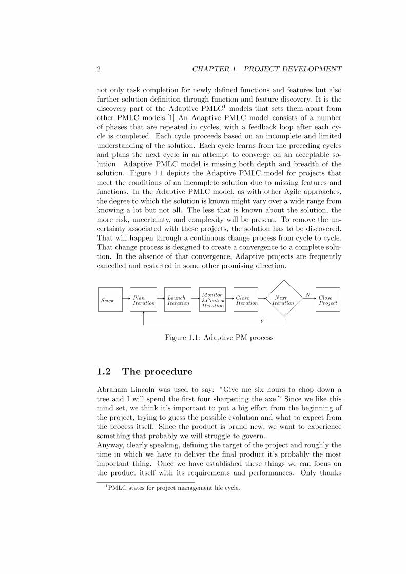
not only task completion for newly defined functions and features but alsofurther solution definition through function and feature discovery. It is thediscovery part of the Adaptive PMLC1 models that sets them apart fromother PMLC models.[1] An Adaptive PMLC model consists of a numberof phases that are repeated in cycles, with a feedback loop after each cy-cle is completed. Each cycle proceeds based on an incomplete and limitedunderstanding of the solution. Each cycle learns from the preceding cyclesand plans the next cycle in an attempt to converge on an acceptable so-lution. Adaptive PMLC model is missing both depth and breadth of thesolution. Figure 1.1 depicts the Adaptive PMLC model for projects thatmeet the conditions of an incomplete solution due to missing features andfunctions. In the Adaptive PMLC model, as with other Agile approaches,the degree to which the solution is known might vary over a wide range fromknowing a lot but not all. The less that is known about the solution, themore risk, uncertainty, and complexity will be present. To remove the un-certainty associated with these projects, the solution has to be discovered.That will happen through a continuous change process from cycle to cycle.That change process is designed to create a convergence to a complete solu-tion. In the absence of that convergence, Adaptive projects are frequentlycancelled and restarted in some other promising direction.
Scope P lanIteration
LaunchIteration
Monitor&ControlIteration Iteration
Close NextIteration
Y
CloseProject
N
Figure 1.1: Adaptive PM process
1.2 The procedure
Abraham Lincoln was used to say: ”Give me six hours to chop down atree and I will spend the first four sharpening the axe.” Since we like thismind set, we think it’s important to put a big effort from the beginning ofthe project, trying to guess the possible evolution and what to expect fromthe process itself. Since the product is brand new, we want to experiencesomething that probably we will struggle to govern.Anyway, clearly speaking, defining the target of the project and roughly thetime in which we have to deliver the final product it’s probably the mostimportant thing. Once we have established these things we can focus onthe product itself with its requirements and performances. Only thanks
1PMLC states for project management life cycle.

1.2. THE PROCEDURE 3
to clear requirements we would be able to understand if we are on theright path, if we are doing well and if we are on time for the delivery.The following Fig. 1.2 is only a preliminary Requirement chart based onmacroscopic and general requirements. In the next sections we will developa new requirement chart listing the technical performances and features ofthe product. So if we are asked to summarize how to develop the project
Figure 1.2: Table of requirements
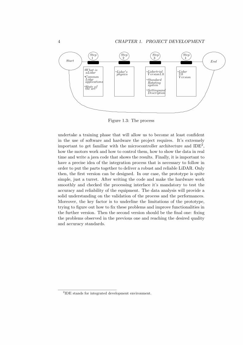
pointing out all the steps and describing the macroscopic phases of if, we caneasily reply explaining Fig. 1.3. In this picture are reported the milestonesof the project. By the continuous check and monitoring of the status of theproject, taking into account the successful engagement of the milestones weare able to understand how we are proceeding. In Fig. 1.4 is showed thetimeline of the whole project. The fist step is related to the acquisition of theinformations. At this stage is fundamental to study the LiDAR technologyby itself and then make a research related to the prior art. Talking aboutthis last topic, we will firstly focus our attention on the market productsand secondly to the open sources projects. The open source communityoffers a huge variety of examples and related projects from which we cantake some inspiration. Moreover, the DIY spirit fits perfectly our idea tokeep low the cost of our platform. In the second stage it is expected toidentify the components which are necessary to manufacture the LiDAR, atleast in its first version. This version will be a learning trial version fromwhich we expect to gather experience and understand the limits and theboundaries of the system. Once we have a precise idea of the equipment, itwill be necessary to understand how to organize our work and necessarily
4 CHAPTER 1. PROJECT DEVELOPMENT
Start
Step1
What is
Common
State of
Step2
Lidar′s
Step3
Lidartrial
Standard
Settingsand
Step4
Lidar
End
aLidar
applications
the art
physics
Lidar
V ersion1.0
Rotatingsystem
Description
2.0V ersion
Figure 1.3: The process
undertake a training phase that will allow us to become at least confidentin the use of software and hardware the project requires. It’s extremelyimportant to get familiar with the microcontroller architecture and IDE2,how the motors work and how to control them, how to show the data in realtime and write a java code that shows the results. Finally, it is important tohave a precise idea of the integration process that is necessary to follow inorder to put the parts together to deliver a robust and reliable LiDAR. Onlythen, the first version can be designed. In our case, the prototype is quitesimple, just a turret. After writing the code and make the hardware worksmoothly and checked the processing interface it’s mandatory to test theaccuracy and reliability of the equipment. The data analysis will provide asolid understanding on the validation of the process and the performances.Moreover, the key factor is to underline the limitations of the prototype,trying to figure out how to fix these problems and improve functionalities inthe further version. Then the second version should be the final one: fixingthe problems observed in the previous one and reaching the desired qualityand accuracy standards.
2IDE stands for integrated development environment.

1.2. THE PROCEDURE 5
TIMELINEAPRIL [4月] MAY [5月] JUNE [6月]
Comps identification04.10
Search appropriate components
Arduino microcontrollerServo control
Lidar Version 1.0Code & hardware
05.10
Test and data
Lidar Version 2.0
05.31
Code & hardware
Test & data
TASK
SubTask
Mile Stone
xx.yyDelivery Date
MARCH [3月]
Info AcquisitionPrior art: market products and opensource platform
03.20
Learning Phase
Processing
Integration
06.31
Figure 1.4: Timeline

6 CHAPTER 1. PROJECT DEVELOPMENT
Chapter 2
Introduction on LiDARSystems
2.1 What is a LiDAR
From the origins of electronics we have always heard about RADAR. Thisdevices is able to detect the position of objects which occupy the spacethanks electromagnetic waves. Only in recent years the RADAR concept hasbeen exploited in the optics field, by achieving an optical RADAR called Li-DAR. In other words, RADAR systems emit radio waves and measure whatbounces back, LiDAR uses light waves. It’s a powerful data collection sys-tem that provides 3-D information for an area of interest or a project area.This device is versatile and suitable for different purposes. Especially in thelast 5 or 10 years the scientific community and a lot of companies have beenfocused on this product trying to imagine possible applications in differentfields of technology.If we want to write on paper a more precise definition we can say that:LiDAR is a surveying method that measures distance to a target by illumi-nating it with a pulsed laser light, and measuring the reflected pulses with asensor. Differences in laser return times and wavelengths can then be usedto make digital 3D-representations of the target.[2]To understand whether LiDAR might be appropriate for our agency’s sur-veying project needs, we will need a thorough understanding of the accuracyand data requirements for the project at hand. By mapping out these criti-cal components in advance we will be able to get a handle on the appropri-ate LiDAR solution, including the hardware, software, and ground control.Someone could ask us why? Because a thorough understanding of the typeof project we are undertaking will help us determine the ground control ofthe project. For example, a corridor mapping project will be conducteddifferently from a county-wide collection. Or more, for example, a mobile-mapping collection is a whole different work from a terrestrial or airborne
7
8 CHAPTER 2. INTRODUCTION ON LIDAR SYSTEMS
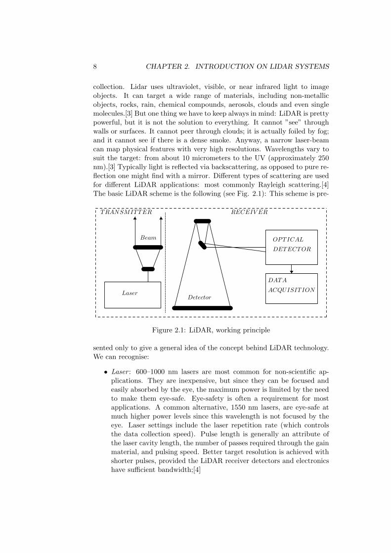
collection. Lidar uses ultraviolet, visible, or near infrared light to imageobjects. It can target a wide range of materials, including non-metallicobjects, rocks, rain, chemical compounds, aerosols, clouds and even singlemolecules.[3] But one thing we have to keep always in mind: LiDAR is prettypowerful, but it is not the solution to everything. It cannot ”see” throughwalls or surfaces. It cannot peer through clouds; it is actually foiled by fog;and it cannot see if there is a dense smoke. Anyway, a narrow laser-beamcan map physical features with very high resolutions. Wavelengths vary tosuit the target: from about 10 micrometers to the UV (approximately 250nm).[3] Typically light is reflected via backscattering, as opposed to pure re-flection one might find with a mirror. Different types of scattering are usedfor different LiDAR applications: most commonly Rayleigh scattering.[4]The basic LiDAR scheme is the following (see Fig. 2.1): This scheme is pre-
Laser
TRANSMITTER
Beam
Detector
OPTICAL
DETECTOR
DATA
ACQUISITION
RECEIV ER
Figure 2.1: LiDAR, working principle
sented only to give a general idea of the concept behind LiDAR technology.We can recognise:
• Laser : 600–1000 nm lasers are most common for non-scientific ap-plications. They are inexpensive, but since they can be focused andeasily absorbed by the eye, the maximum power is limited by the needto make them eye-safe. Eye-safety is often a requirement for mostapplications. A common alternative, 1550 nm lasers, are eye-safe atmuch higher power levels since this wavelength is not focused by theeye. Laser settings include the laser repetition rate (which controlsthe data collection speed). Pulse length is generally an attribute ofthe laser cavity length, the number of passes required through the gainmaterial, and pulsing speed. Better target resolution is achieved withshorter pulses, provided the LiDAR receiver detectors and electronicshave sufficient bandwidth;[4]
2.1. WHAT IS A LIDAR 9
• Scanner and optics: How fast images can be developed is also affectedby the speed at which they are scanned. There are several options toscan the azimuth and elevation, including dual oscillating plane mir-rors, a combination with a polygon mirror and a dual axis scanner.Optic choices affect the angular resolution and range that can be de-tected. A hole mirror or a beam splitter are options to collect a returnsignal;
• Photo-detector and receiver electronics: Two main photo-detector tech-nologies are used in Lidar. The first is solid state photo-detectors, suchas silicon avalanche photo-diodes, or photo-multipliers. The sensitiv-ity of the receiver is another parameter that has to be balanced in aLidar system design;
• Position and navigation systems: LiDAR sensors that are mounted onmobile platforms such as airplanes or satellites require instrumentationto determine the absolute position and orientation of the sensor. Suchdevices generally include a Global Positioning System receiver and anInertial Measurement Unit (IMU).
Talking about traditional and conventional LiDAR is good to get familiarwith some specific language which can help to understand better what justsaid:
• Repetition Rate: this is the rate at which the laser is pulsing, and it ismeasured in kilohertz (KHz). Laser emits extremely quick pulses, soit’s important to check that all the equipments, such as trans-receiverand receiver are able to operate at the maximum laser pulsing speed;
• Scan frequency : while the laser is pulsing, the scanner is oscillating,or moving back and forth. The scan frequency will tell how fast thescanner is oscillating. A mobile system has a scanner that rotatescontinuously in a 360 degree fashion, but most airborne scanners moveback and forth.
• Scan angle: this is measured in degrees and is the distance that thescanner moves from one end to the other. We will adjust the angledepending on the application and the accuracy of the desired dataproduct;
• Flying attitude: it is not a surprise that the farther the platform isfrom the target, the lower the accuracy of the data and the less densethe points will be that define the target area. That’s why for airbornesystems, the flying attitude is so important. This aspect in our caseit’s less relevant since we are interested in short range applications;

10 CHAPTER 2. INTRODUCTION ON LIDAR SYSTEMS
• Nominal point spacing (NPS): The rule is simple enough the morepoints that are hit in the collection, the better we will define the tar-gets. The point sample spacing varies depending on the application.It’s also good to keep in mind that LiDAR systems are random sam-pling systems. Although it’s not possible to determine exactly wherethe points are going to hit on the target area. The only thing that ispossible to do is that we can decide how many times the target areasare going to be hit, so for example we can choose a higher frequencyof points to better define the targets.
• Cross track resolution: this is the spacing of the pulses from the LiDARsystem in the scanning direction, or perpendicular to the direction thatthe platform is moving;
• Swath: this is the actual distance of the area of coverage for the LiDARsystem. It can vary depending on the scan angle. Mobile LiDAR has aswath, too, but it is usually fixed and depends on the particular sensor.For these systems, though, you might not hear the word ”swath” itmay instead be referred to as the ”area of coverage” and will varydepending on the repetition rate of the sensor;
• Overlap: it’s the amount of redundant area that is covered betweenflight lines or swaths within an area of interest. Overlap is not a wastedeffort, because sometimes it provides more accuracy.[3]
So, the accuracy of the system depends not only on laser’s feature buteven on the proprieties of the revelation and the system in general. Here wehave to be honest and add some more informations. Actually, during thedevelopment of this work, we are basically interested in mechanical scan-ning systems. Even though mechanical rotational detection systems havesome limits and disadvantages, they’re quite easy to implement and de-velop. One of the major drawbacks is the fact that the scanning speed isa limit to the performances of the LiDAR and at the same time reducesthe rotating components life, causing fatalities and premature failure. Aswith just about any technology that requires precision you cannot count onLiDAR collection without proper sensor calibration. All sensors should becalibrated routinely, and calibration is recommended after every installationinto a platform. How you calibrate depends on the system and the LiDARprovider, but the results are similar. Terrestrial LiDAR scanners, however,have self calibrations that take place before every collection. In addition,all LiDAR systems (whether in the air or on the ground) are initially cal-ibrated by the manufacturer in a lab and during field trials. Whenever ahardware component is repaired or replaced on a LiDAR sensor head, thesystem should be recalibrated. It is also important to remember that everyfurther modification and adjustment of the system brings to a revision andcheck up status of the new configuration.
2.2. LIDAR APPLICATIONS 11
2.2 Lidar Applications
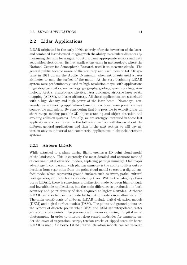
LiDAR originated in the early 1960s, shortly after the invention of the laser,and combined laser-focused imaging with the ability to calculate distances bymeasuring the time for a signal to return using appropriate sensors and dataacquisition electronics. Its first applications came in meteorology, where theNational Center for Atmospheric Research used it to measure clouds. Thegeneral public became aware of the accuracy and usefulness of LiDAR sys-tems in 1971 during the Apollo 15 mission, when astronauts used a laseraltimeter to map the surface of the moon. At the very beginning LiDARsystem were predominantly used in high-resolution maps, with applicationsin geodesy, geomatics, archaeology, geography, geology, geomorphology, seis-mology, foretry, atmospheric physics, laser guidance, airborne laser swathmapping (ALSM), and laser altimetry. All those applications are associatedwith a high density and high power of the laser beam. Nowadays, con-versely, we are seeking applications based on low laser beam power and eyecompatible and safety. By considering that it’s possible to exploit Lidar onshort range, making possible 3D object scanning and object detection andavoiding collision systems. Actually, we are strongly interested in these lastapplications and solutions. In the following part we will discuss about thedifferent general applications and then in the next section we will pay at-tention only to industrial and commercial applications in obstacle detectionsystems.
2.2.1 Airborn LiDAR
While attached to a plane during flight, creates a 3D point cloud modelof the landscape. This is currently the most detailed and accurate methodof creating digital elevation models, replacing photogrammetry. One majoradvantage in comparison with photogrammetry is the ability to filter out re-flections from vegetation from the point cloud model to create a digital sur-face model which represents ground surfaces such as rivers, paths, culturalheritage sites, etc., which are concealed by trees. Within the category of air-borne LiDAR, there is sometimes a distinction made between high-altitudeand low-altitude applications, but the main difference is a reduction in bothaccuracy and point density of data acquired at higher altitudes. AirborneLiDAR can also be used to create bathymetric models in shallow water.[5]The main constituents of airborne LiDAR include digital elevation models(DEM) and digital surface models (DSM). The points and ground points arethe vectors of discrete points while DEM and DSM are interpolated rastergrids of discrete points. The process also involves capturing of digital aerialphotographs. In order to interpret deep seated landslides for example, un-der the cover of vegetation, scarps, tension cracks or tipped trees air borneLiDAR is used. Air borne LiDAR digital elevation models can see through
12 CHAPTER 2. INTRODUCTION ON LIDAR SYSTEMS
the canopy of forest cover, perform detailed measurements of scarps, erosionand tilting of electric poles.[6] Airborne lidar data is processed using a tool-box called Toolbox for Lidar Data Filtering and Forest Studies (TIFFS) forlidar data filtering and terrain study software. The data is interpolated todigital terrain models using the software. The laser is directed at the regionto be mapped and each point’s height above the ground is calculated bysubtracting the original z-coordinate from the corresponding digital terrainmodel elevation. Based on this height above the ground the non-vegetationdata is obtained which may include objects such as buildings, electric powerlines, flying birds etc. The rest of the points are treated as vegetation andused for modeling and mapping. Within each of these plots, lidar metricsare calculated by calculating statistics such as mean, standard deviation,skewness, percentiles, quadratic mean etc. ;
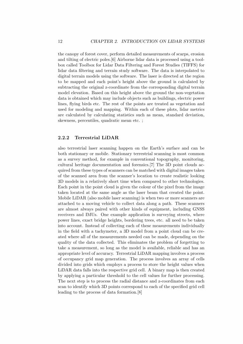
2.2.2 Terrestrial LiDAR
also terrestrial laser scanning happen on the Earth’s surface and can beboth stationary or mobile. Stationary terrestrial scanning is most commonas a survey method, for example in conventional topography, monitoring,cultural heritage documentation and forensics.[7] The 3D point clouds ac-quired from these types of scanners can be matched with digital images takenof the scanned area from the scanner’s location to create realistic looking3D models in a relatively short time when compared to other technologies.Each point in the point cloud is given the colour of the pixel from the imagetaken located at the same angle as the laser beam that created the point.Mobile LiDAR (also mobile laser scanning) is when two or more scanners areattached to a moving vehicle to collect data along a path. These scannersare almost always paired with other kinds of equipment, including GNSSreceivers and IMUs. One example application is surveying streets, wherepower lines, exact bridge heights, bordering trees, etc. all need to be takeninto account. Instead of collecting each of these measurements individuallyin the field with a tachymeter, a 3D model from a point cloud can be cre-ated where all of the measurements needed can be made, depending on thequality of the data collected. This eliminates the problem of forgetting totake a measurement, so long as the model is available, reliable and has anappropriate level of accuracy. Terrestrial LiDAR mapping involves a processof occupancy grid map generation. The process involves an array of cellsdivided into grids which employs a process to store the height values whenLiDAR data falls into the respective grid cell. A binary map is then createdby applying a particular threshold to the cell values for further processing.The next step is to process the radial distance and z-coordinates from eachscan to identify which 3D points correspond to each of the specified grid cellleading to the process of data formation.[8]

2.2. LIDAR APPLICATIONS 13
2.2.3 Autonomous vehicles
From the official NTSB’s (National Transportation Security Board - US)website we can actually see that an average of 38000 [12] people per yearloose their life on the american roads due to car accidents and fatalities. Toput that in perspective, that’s more than a Boeing 737 falling out of thesky five times per week in a year. Could we accept something similar inthe aviation? Probably the answer is no. So, this is the main reason whyLiDAR technology has to be exploited in autonomous driving car; but safetyis not the unique reason. The second theme is related to health and money:taking into account the average commuter in America, which is around 50minutes per worker per day, you multiply by the number of daily workers,120 million, you get 6 billion minutes per day lost by the american workerssat in traffic. If you compare this time to the the average life expectancy,around 70 years, you get 162 lifetimes waisted in the traffic jam per day. Another time, this is not social acceptable. And last but not least important,there’s a reason related to diversity and inclusion: self driving car could helpto improve the mobility of disable people.Moreover, as per the latest World Health Organization reports, road trafficaccidents account for 1.25 million deaths each year. In fact, according to anestimate, by the year 2030 road traffic accidents will be the 7th major causeof death around the world. It is in this context that the UN’s 2030 Agendafor Sustainable Development becomes even more important. A target hasbeen set to reduce the number of traffic accident deaths by 50% by 2020. Inlight of these statistics, it is clear to see why the use of LiDAR technologyis critical. Unlike other types of sensors or telematics currently available,LiDAR has improved capabilities when it comes to the detection of objects,even in cases where there is a complete absence of light. LiDAR’s features,which include a blind spot monitoring system, adaptive cruise control, alongwith a collision avoidance system and pedestrian protection system, are notonly better than the features of other sensors, but are also far more consis-tent and reliable. Analysts at Technavio predict that the global automotiveLiDAR sensors market will see a CAGR of more than 34% by 2020.May use LiDAR for obstacle detection and avoidance to navigate safelythrough environments, using rotating laser beams. Cost map or point cloudoutputs from the LiDAR sensor provide the necessary data for robot soft-ware to determine where potential obstacles exist in the environment andwhere the robot is in relation to those potential obstacles. Examples of com-panies that produce LiDAR sensors commonly used in robotics or vehicleautomation are Sick and Hokuyo. Examples of obstacle detection and avoid-ance products that leverage LiDAR sensors are the Autonomous Solution,Inc. Forecast 3D Laser System and Velodyne HDL-64E. This is actually theworld in which we want to dive deeply. So in the next section we will lookat the products now available on the market, painting the ”affresco” of the

14 CHAPTER 2. INTRODUCTION ON LIDAR SYSTEMS
so called prior art. The very first generations of automotive adaptive cruisecontrol systems used only LiDAR sensors and it is expected a more intenseuse of these technologies in the next future.
2.2.4 Urban Planning
in this growing phase of urbanization and industrialization there is an emer-gent need of proper town planning systems. The 3D city models in urbanareas are essential for many applications, such as military operations, dis-aster management, mapping of buildings and their heights, simulation ofnew buildings, updating and keeping cadastral data, change detection andvirtual reality. Urban, city, or town planning is the discipline of land useplanning which explores several aspects of the built and social environmentsof municipalities and communities. The urban areas in the developing worldare under constant pressure of a growing population.[9] Efficient urban in-formation system is a vital pre-requisite for planned development. It isthought that LiDAR application to urbanization plans will bring to a moresustainable and efficient growth of a city. In traffic line design area, LiDARtechnology offers a high precision DEM (Digital Elevation Model) for roadand railway design, to facilitate route design and the calculation of earthwork quantity. Besides, it is also of great application significance in routedesign of communication network, oil pipe, air pipe. In digital city project,a ”digital city” system can be established and perfected by combining thehigh-precision DEM and GPS of LiDAR, and the data can be updated realtime therewith.[11] It is expected that LiDAR systems will be massivelyused to plan the development of the cities of the future, to integrate newinfrastructure in existing contexts, taking into account sustainability andreal constraints due to environment, population and other key factors. Inother words, the rational urban densification and optimization, as well asthe development and construction of new buildings, streets, subway andtram lines and innovative means of transportation is strictly related to theimplementation of this technology.
2.2.5 Energy
combining LiDAR technology and GIS (Geographic Information System) ispossible to develop a method for predicting city-wide electricity gains fromphotovoltaic panels based on detailed 3D urban massing models combinedwith Daysim-based hourly irradiation simulations, typical meteorologicalyear climactic data and hourly calculated rooftop temperatures. The re-sulting data can be combined with online mapping technologies and searchengines as well as a financial module that provides building owners inter-ested in installing a photovoltaic system on their rooftop with meaningfuldata regarding spatial placement and informations.[10] So, in this sense Li-
2.3. STATE OF THE ART LIDAR SCANNING TECHNOLOGY 15
DAR could help the diffusion of RES (Renewable energy sources) in a moreefficient and rational way. This is only a simple example of what is possibleto conceive in the energy world thanks to LiDAR technology. An other im-portant and relevant example is related to power transmission lines statusmonitoring. In electric power transmission area, it can make for the laying,maintenance and management of power grid. In the link of electric powerline design, the terrains and geographic features within the entire line designarea can be learned about based on LiDAR data. Especially in areas withthick trees, the area and amount of trees to be cut down can be estimated.In the link of power lines repair and maintenance, the height of line at anylocation can be measured and calculated based on the LiDAR data pointson the electric power line and the elevation of corresponding exposed spoton the ground, which can facilitate repair and maintenance.[11] Not onlyOther relevant applications are missing for a time issues such as agriculture,archeology or biology. Who is writing doesn’t want to explain in detail theseapplications.
2.3 State of the art LiDAR scanning Technology
So, as said, this section is dedicated to the prior art. In other words theunderstanding of the most important players on the LiDAR market at themoment, also called incumbent, and a focus on the prominent players or newcomers.
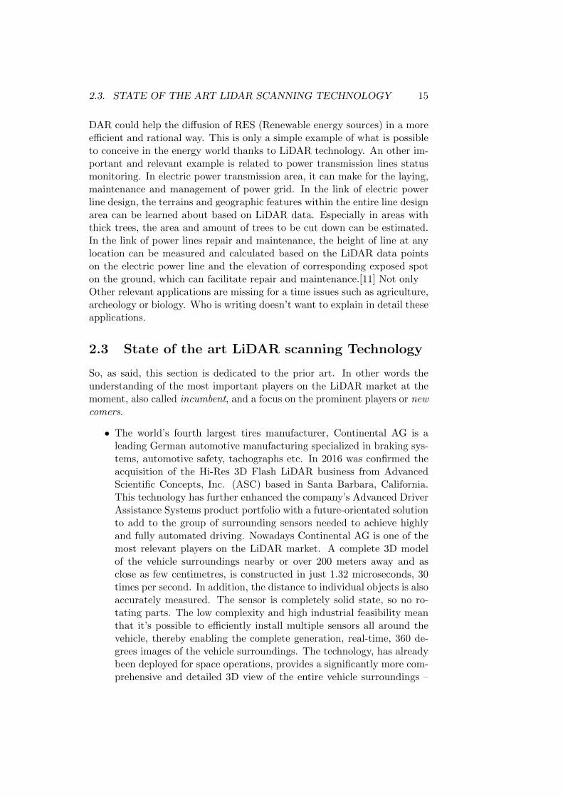
• The world’s fourth largest tires manufacturer, Continental AG is aleading German automotive manufacturing specialized in braking sys-tems, automotive safety, tachographs etc. In 2016 was confirmed theacquisition of the Hi-Res 3D Flash LiDAR business from AdvancedScientific Concepts, Inc. (ASC) based in Santa Barbara, California.This technology has further enhanced the company’s Advanced DriverAssistance Systems product portfolio with a future-orientated solutionto add to the group of surrounding sensors needed to achieve highlyand fully automated driving. Nowadays Continental AG is one of themost relevant players on the LiDAR market. A complete 3D modelof the vehicle surroundings nearby or over 200 meters away and asclose as few centimetres, is constructed in just 1.32 microseconds, 30times per second. In addition, the distance to individual objects is alsoaccurately measured. The sensor is completely solid state, so no ro-tating parts. The low complexity and high industrial feasibility meanthat it’s possible to efficiently install multiple sensors all around thevehicle, thereby enabling the complete generation, real-time, 360 de-grees images of the vehicle surroundings. The technology, has alreadybeen deployed for space operations, provides a significantly more com-prehensive and detailed 3D view of the entire vehicle surroundings –
16 CHAPTER 2. INTRODUCTION ON LIDAR SYSTEMS
both during the day and at night – and works reliably even in adverseweather conditions. Mass production will start at the end of 2019 andthe product will be on the market in the early 2020, as scheduled.The price is not known yet, but rumors say around 7000 dollars (eventhough we don’t know if this could be a realistic number).
Figure 2.2: 3D flash LIDAR by Continental AG [13]
• Cosworth, the leading designer and manufacturer of high performanceengines and end-to-end automotive technologies, demonstrated a pro-totype of solid state LiDAR sensor technology as part of the officialopening of its new state-of-the-art manufacturing center and NorthAmerican Headquarters in Shelby Township, last June.[14] Media andinvited guests witnessed a demonstration of a solid state LiDAR tech-nology. Having no moving parts, the technology is designed and builtto provide stability that will meet the stringent automotive standardsfor reliability. At the grand opening of North American manufac-turing center they demonstrated the stability, precision, distance andfield of view that are necessary to make autonomous or assisted drivingsafe. With a minimum of 3,200 lasers, a clear 120-degree filed of viewand 200 meter range, it is believed that this solution could be a gamechanger for automotive sensor technology. Right now we have no moreinformation related to the product, large scale industrial productionand especially the price the LiDAR will be sold on the market.[14]Anyway, since the author of this work consider that manufacturer andproduct interesting it has been reported here. More information in thefollowing months.
2.3. STATE OF THE ART LIDAR SCANNING TECHNOLOGY 17
Description Value
Wavelenght 830 nmMaximum pulse energy 5 nJPulse Duration 4 nsPulse repetition frequency 2.16 MHzBeam divergence (FWHM, full angle) 0.4 mradMirror rotation 30 HzBase rotation 2.5 mHz
Table 2.1: BLK360 Laser Specs
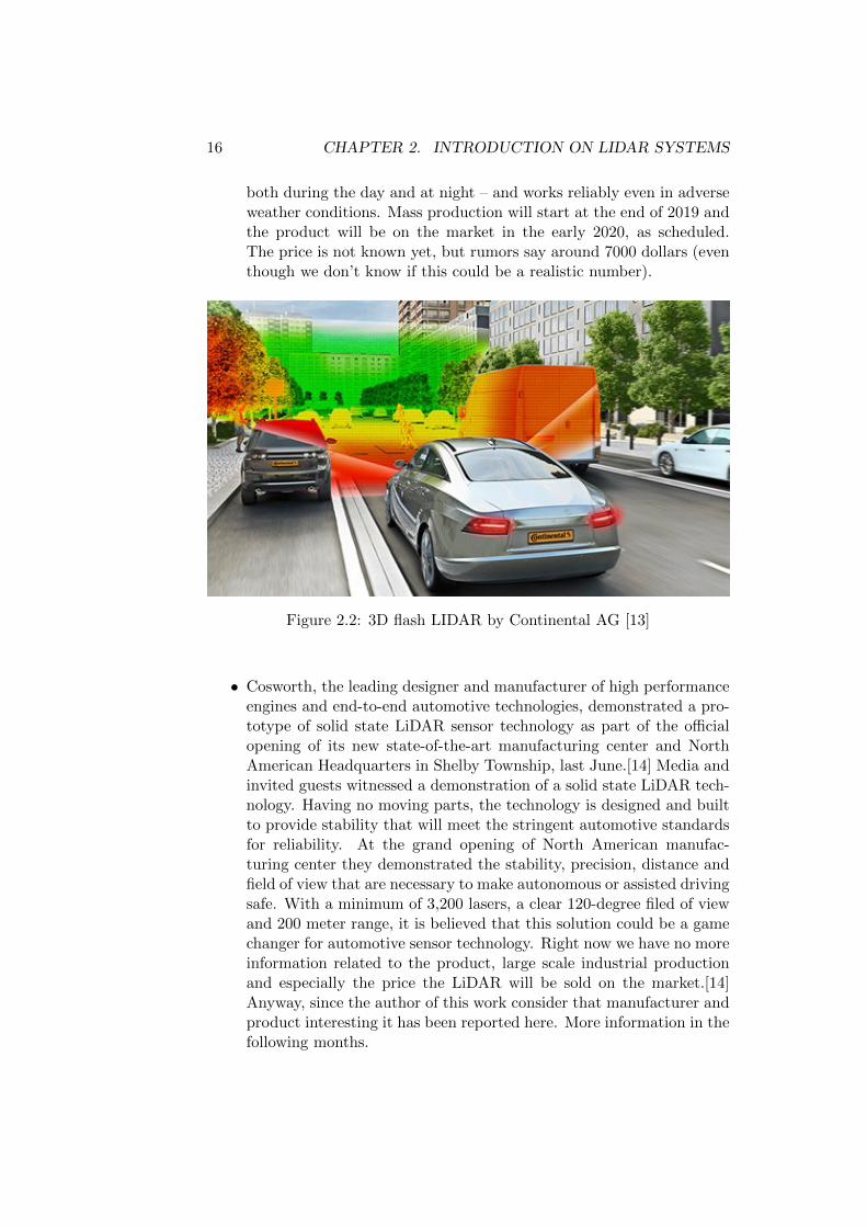
• In this section is presented one of the LiDAR based products which Ibelieve is extremely interesting since its aim is similar to the one thatwe have developed (later in this work we will talk about that exten-sively). In detail we are talking about LEICA BLK360 which is usedto digitalize interiors and recreate the respective 3D representation.The Leica BLK360 captures the world around you with full-colourpanoramic images overlaid on a high-accuracy point cloud. Simple touse with just the single push of one button, the BLK360 is the small-est and lightest of its kind. Anyone who can operate an iPad can nowcapture the world around them with high resolution 3D panoramicimages. Using the ReCap Pro mobile app, the BLK360 streams imageand point cloud data to iPad. The app filters and registers scan data inreal time. After capture, ReCap Pro enables point cloud data transferto a number of CAD, BIM, VR and AR applications. The integrationof BLK360 and Autodesk software dramatically streamlines the real-ity capture process thereby opening this technology to non-surveyingindividuals. In few points:
– Allows you to scan in high, standard and fast resolutions;
– Weighs 1kg / Size 165 mm tall x 100 mm diameter;
– Less than 3 minutes for full-dome scan (in standard resolution)and 150 MP spherical image generation;
– 360,000 laser scan pts/se
– HDR and thermal imaging
Table 2.1 reports BLK360 Laser propriety.
The laser incorporated in the product produces an invisible beam whichemerges from the rotating mirror. The laser product described in this sectionis classified as laser class 1 in accordance with IEC prescriptions. This

18 CHAPTER 2. INTRODUCTION ON LIDAR SYSTEMS
Figure 2.3: Leica BLK360
products is safe under reasonably foreseeable conditions of operation. Theprice for this product is quite prohibitive, around 16000$. Leica BLK360can offer amazing performances and results but the price it’s a great obstacleto its mainstream diffusion.
So, this is a brief presentation of the products I believe are more promis-ing and interesting on the market. As I have said before the one we are moreinterested in is Leica BLK360, because as specifications and characteristicsof the products is the closest to the LiDAR platform we have developed.In fact we focused our attention on interior scanning and 3D environmentreconstruction. For sure our platform’s performance will be not comparablewith an industrial product which costs several thousands of dollars. Just tobe clear our budget is around 250$. Anyway, we consider the low budget apositive aspect, in fact we want to show that is possible to get a good result(high density point cloud) even though a less powerful hardware is used. Inthis case it will be necessary to optimize and deploy at its best the hardwarewe have in our hands. One of the biggest differences between our versionand Leica’s version will be for sure the acquisition speed: actually, it is saidthat the commercial product is able to get a 360 degrees representation ofthe environment roughly in 3 minutes. Probably, our prototype could scanthe environment for sure at a slower speed, maybe 6 times slower. We be-lieve, though, is still ok, considering that time is not the principal driver forour project.
2.4. LIDAR PROJECT SCOPE 19
2.4 LiDAR Project Scope
In this section a deeper focus on the description of the LiDAR platform’sscope is given to the reader. A partial portrait or canvas has been presentedin §Chap. 1, §Sec. 1.2. Right now, we want to underline that the prototypeunder the magnifying glass will provide:
• high resolution & high density Point Cloud;
• to each point will be assigned a colour, considering the distance fromthe sensor;
• a navigation system based on Java which will allow the user to see inreal time the scanning result and translate and rotate the Point Cloud.
As we have already mentioned, at the moment the scanning speed it’s nota big issue. At first our attention will be totally focused on getting a highdensity and high resolution Point Cloud. Only, then we will change our fo-cus on getting a higher scanning speed. The development of the final versionis a complex problem, achievable only through incremental steps. First ofall, it’s necessary to get familiar with the concept of LiDAR systems, howdo they work, their specifications, the safety rules needed to operate thesesystems. Then we will move towards the first prototype which is a simpleLiDAR platform, more similar to a turret able to roughly scan the 3D spacewhich surrounds us, without any pretension to be accurate or detailed. Theaim of this first step is to get and accumulate experience, show to be familiarwith MCU control and writing algorithm able to execute what is intended.In this first operative phase is necessary to understand that even a smallproject is constitute by different sub-projects and it’s highly recommendedto schedule precisely the different parts and then assemble meticulously thewhole system solving in a smart way the integration problems. Only then itwill be possible to extensively develop the more advance and final version.Starting from the limits and the problems emerged during phase 1, it willbe possible to study and conceive engineering solutions able to push forwardthe performances of the machine and eventually get a better, more realisticand industrial exploitable result.Last but not the least during the whole process in essential to test smallparts of the platform in the Lab in order to validate components specifica-tions, new possible solutions or the real boundaries of the platform itself.So the engineering development is strictly linked to the test phase and thepragmatic approach to problems.In the next Chapter will be present the basic knowledge, necessary to un-derstand how the following prototypes will work. We will pay attention todetails and protocols, as for example how the data transmission betweensensor and MCU works and other important topics. Eventually, then, it willbe possible to present how the LiDAR platforms has been made.

20 CHAPTER 2. INTRODUCTION ON LIDAR SYSTEMS
Chapter 3
Fundamentals on LiDAR
As we have said in the previous sections, especially the realization of this firstplatform is essential to get confident with the equipment, and in particularstudy more deeply the interaction between hardware and software. Thelanguage necessary to control the MCU or better the micro controller thatwe’ll use constitutes a completely new barrier. So, for this first period it’snecessary to study and practice what’s written on books, web manuals andtutorials.In this Chapter will be reported and explained basic principles and howthings work; in particular:
• Sensor;
• Micro-Controller (Arduino);
• Servo Motors;
• Processing v3;
3.1 The Sensor
When space and weight requirements are tight, the LiDAR-Lite v3 soars.It’s the ideal compact, high-performance optical distant measurement sensorsolution for drone, robot or unmanned vehicle applications. Using a singlechip signal processing solution along with minimal hardware, this highlyconfigurable sensor can be used as the basic building block for applicationswhere small size, light weight, low power consumption and high performanceare important factors. Featuring all of the core features of the popularLiDAR-Lite v2, this easy-to-use 40 meter laser-based sensor uses about 130milliamps during an acquisition. It is user-configurable so you can adjustbetween accuracy, operating range and measurement time. It’s reliable,powerful ranging and it’s a versatile proximity sensor. This is LIDAR-Litev3, a compact optical distance measurement sensor from Garmin. Each
21

22 CHAPTER 3. FUNDAMENTALS ON LIDAR
Specifications Measurements
Size (l x w x h) 20 x 48 x 40 mmWeight 22 gOperating Temperature -20 to 60 C
Table 3.1: Phisical Propriety Garmin Lidar Lite v3
Specifications Measurements
Power5 Vdc nominal4.5 Vdc min., 5.5 Vdc max.
Current105 mA idle135 mA continuous operations
Table 3.2: Electrical Propriety Garmin Lidar Lite v3
LiDAR-Lite v3 features an edge-emitting, 905nm (1.3 watts), single-stripelaser transmitter, 4 m Radian x 2 m Radian beam divergence, and an opticalaperture of 12.5mm. The third version of the LiDAR-Lite still operates at5V DC with a current consumption rate of <100mA at continuous operation.On top of everything else, it can be interfaced via I2C or PWM with theincluded 200mm accessory cable.Note: CLASS 1 LASER PRODUCT CLASSIFIED EN/IEC 60825-1 2014.This product is in conformity with performance standards for laser productsunder 21 CFR 1040, except with respect to those characteristics authorizedby Variance Number FDA-2016-V-2943 effective September 27, 2016.
3.1.1 Technology and Operations
This device measures distance by calculating the time delay between thetransmission of a Near Infra-red laser and its reception after reflecting off atarget. This translates into distance using the known speed of light. Theunique signal processing approach transmits a coded signature and looksfor that signature in the return, which allows for highly reflective detectionwith eye-safe laser power levels. Proprietary signal processing techniques areused to achieve high sensitivity, speed and accuracy in a small, low powerand low-cost system.To take a measurement, this device first performs a receiver bias correctionroutine, correcting for changing ambient light levels and allowing maximumsensitivity. Then the device sends a reference signal directly from the trans-

3.1. THE SENSOR 23
mitter to the receiver. It stores the transmit signature, sets the time delayfor ”zero” distance, and recalculates this delay periodically after several mea-surements. Next, the device initiates a measurements by performing a seriesof acquisitions. Each acquisition is a transmission of the main laser signalwhile recording the return signal at the receiver. If there is a signal match,the result is stored in memory as a correlation record. The next acquisitionis summed with the previous result. When an object at a certain distancereflects the laser signal back to the device, these repeated acquisitions causea peak to emerge, out of the noise, at the corresponding distance locationin the correlation record.The device integrates acquisitions until the signal peak in the correlationrecord reaches a maximum value. If the returned signal is not strong enoughfor this to occur, the device stops at the predetermined maximum acquisi-tion count. Signal strength is calculated from the magnitude of the signalrecord peak and a valid signal threshold is calculated from the noise floor.If the peak is above the threshold the measurements is considered valid andthe device will calculate the distance, otherwise it will report 1 cm. Whenbeginning the next measurement, the device clears the signal and starts thesequence again.[15]
3.1.2 Interface
Initialization On power-up or reset, the device performs a self-test se-quence and initializes all registers with default values. After roughly 22 msdistance measurements can be taken with the I2C interface or the ModeControl Pin. So before explaining how LiDAR Lite v3’s I2C works it’s bet-ter to give to the reader some basic and general informations related to I2Citself. Only then it will be possible to understand clearly how the LiDARdata transmission works.[15]
I2C description I2C-bus compatible ICs don’t only assist designers, theyalso give a wide range of benefits to equipment manufacturers because:
• The simple 2-wire serial I2C-bus minimizes interconnections so ICshave fewer pins and there are not so many PCB tracks; result - smallerand less expensive PCBs;
• The completely integrated I2C-bus protocol eliminates the need foraddress decoders and other ’glue logic’;
• The multi-master capability of the I2C-bus allows rapid testing andalignment of end-user equipment via external connections to an assembly-line;

24 CHAPTER 3. FUNDAMENTALS ON LIDAR
• The availability of I2C-bus compatible ICs in SO (small outline), VSO(very small outline) as well as DIL packages reduces space requirementseven more.
These are just some of the benefits. In addition, I2C-bus compatible ICs in-crease system design flexibility by allowing simple construction of equipmentvariants and easy upgrading to keep designs up-to-date. In this way, an en-tire family of equipment can be developed around a basic model. Upgradesfor new equipment, or enhanced-feature models (i.e. extended memory, re-mote control, etc.) can then be produced simply by clipping the appropriateICs onto the bus. If a larger ROM is needed, it’s simply a matter of selectinga micro-controller with a larger ROM. As new ICs supersede older ones, it’seasy to add new features to equipment or to increase its performance bysimply unclipping the outdated IC from the bus and clipping on its succes-sor.For 8-bit oriented digital control applications, such as those requiring mi-crocontrollers, certain design criteria can be established:
• A complete system usually consists of at least one microcontroller andother peripheral devices such as memories and I/O expanders;
• The cost of connecting the various devices within the system must beminimized;
• A system that performs a control function doesn’t require high-speeddata transfer;
• Overall efficiency depends on the devices chosen and the nature of theinterconnecting bus structure.
To produce a system to satisfy these criteria, a serial bus structure is needed.Although serial buses don’t have the throughput capability of parallel buses,they do require less wiring and fewer IC connecting pins. However, a bus isnot merely an interconnecting wire, it embodies all the formats and proce-dures for communication within the system. Devices communicating witheach other on a serial bus must have some form of protocol which avoidsall possibilities of confusion, data loss and blockage of information. Fastdevices must be able to communicate with slow devices. The system mustnot be dependent on the devices connected to it, otherwise modifications orimprovements would be impossible. A procedure has also to be devised todecide which device will be in control of the bus and when. And, if differentdevices with different clock speeds are connected to the bus, the bus clocksource must be defined. All these criteria are involved in the specificationof the I2C-bus.The I2C-bus supports any IC fabrication process (NMOS, CMOS, bipolar).Two wires, serial data (SDA) and serial clock (SCL), carry information
3.1. THE SENSOR 25
between the devices connected to the bus. Each device is recognized bya unique address (whether it’s a microcontroller, LCD driver, memory orkeyboard interface) and can operate as either a transmitter or receiver, de-pending on the function of the device. Obviously an LCD driver is only areceiver, whereas a memory can both receive and transmit data. In additionto transmitters and receivers, devices can also be considered as masters orslaves when performing data transfers. A master is the device which initi-ates a data transfer on the bus and generates the clock signals to permitthat transfer. At that time, any device addressed is considered a slave.[16]
I2C Lidar Lite Interface This device has a 2-wire, I2C-compatible serialinterface. It can be connected to an I2C bus as a slave device, under thecontrol of an I2C master device. It supports 400 kHz Fast Mode data trans-fer. The I2C bus operates internally at 3.3 Vdc. An internal level shifterallows the bus to run at the maximum of 5 Vdc. Internal 3k ohm pull-upresistors ensure this functionality and allow for simple connection to the I2Chost. The device has a 7-bit slave address with the default value of 0x62.The effective 8 bit-bit I2C address is 0x64 write and 0xC5. The device willnot respond to a general call. Support is not provided for 10-bit addressing.The sensor module has a 7-bit slave address with a default value of 0x62 inhexadecimal notation. The effective 8 bit I2C address is: 0x64 write, 0x65read. The device will not presently respond to a general call. Please notesome additional informations:
• This device does not work with repeated START conditions. It mustfirst receive a STOP condition before a new START condition;
• The Ack and NACK item are responses from the master device to theslave device;
• The last NACK in the read is technically optional, but the formal I2Cprotocol states that the master shall not acknowledge the last byte.
So, the I2C serial bus protocol operates as follow:
• The master initiates data transfer by establishing a start condition,which is when a high-to-low transition on the SDA line occurs whileSCL is high. The following byte is the address byte, which consists ofthe 7-bit slave address followed by the read/write bit with zero stateindicating a write request. A write operation is used as the initial stageof both read and write transfer. If the slave address corresponds tothe module’s address the unit responds by pulling SDA low during theninth clock pulse (this is termed the acknowledge bit). At this stage,all other devices on the bus remain idle while the selected device waitsfor data to be written to or read from its shift requester;

26 CHAPTER 3. FUNDAMENTALS ON LIDAR
Figure 3.1: LiDAR Lite I2C read/write operations
• Data is transmitted over the serial bus in sequences of ninth clockpulses (eight data bits followed by an acknowledge bit). The transitionon the SDA line must occur during the low period of SCL and remainstable during the high period of SCL;
• An 8 bit data byte following the address loads the I2C control the reg-ister with the address of the control register to be read along with flagsindicating if auto increment of the addressed control register is desiredwith successive reads or writes; and if access to the internal micro orexternal correlation process register space is requested. Bit locations5:0 contain the control register address while bit 7 enables the auto-matic increment of control register with successive data blocks. Bitposition 6 selects correlation memory external to the micro-controllerif set. (Presently an advanced feature);
• If a read operation is requested, a stop bit is issued by the master atthe completion of the first data frame followed by the initiation of anew start condition, slave address with the read bit set (one state).The new address byte is followed by the reading of the one more databytes succession. After the slave has acknowledged receipt of a validaddress, data read operations proceed by the master releasing the I2C

3.2. ARDUINO 27
Specifications Measurements
Range (70% reflective Target) 40 mResolution ± 1 cmAccuracy <5 m ± 2.5 cm
Accuracy ≥ 5 m
± 10 cmMean± 1% of maximum distanceRipple± 1% of maximum distance
Update Rate (70% reflective Target)270 Hz typical650 Hz fast mode>1000 Hz Short range only
Repetition Rate50 Hz default500 Hz max
Table 3.3: Garmin Lidar Lite v3 Performances
Specifications Measurements
Wavelength 905 nm (nominal)Total Laser Power (peak) 1.3 WMode of operation Pulsed (256 pulsed max. pulse train)Pulse width 0.5 µs (50% duty cycle)Pulse train repetition frequency 10-20 kHz (nominal)Energy per pulse < 280 nJBeam Diameter at laser aperture 12 x 2 mmDivergence 8 m Radian
Table 3.4: Laser Propriety Garmin Lidar Lite v3
data line continuously clocking SCL. At the completion of the receiptof a data byte, the master must strobe the acknowledge bit beforecontinuing the read cycle;
• For a write operation to proceed, Step 3 is followed by one or more 8 bitdata blocks with acknowledges provided by the slave at the completionof each successful transfer. At the completion of the transfer cycle astop condition is issued by the master terminating operation.[15]
3.2 Arduino
Arduino Uno is a microcontroller board based on the ATmega328P. It has14 digital input/output pins (of which 6 can be used as PWM outputs), 6

28 CHAPTER 3. FUNDAMENTALS ON LIDAR
Microcontroller ATmega328P
Operating Voltage 5VInput Voltage (recommended) 7-12VInput Voltage (limit) 6-20VDigital I/O Pins 14 (of which 6 provide PWM output)PWM Digital I/O Pins 6Analog Input Pins 6DC Current per I/O Pin 20 mADC Current for 3.3V Pin 50 mA
Flash Memory32 KB (ATmega328P)of which 0.5 KB used by bootloader
SRAM 2 KB (ATmega328P)EEPROM 1 KB (ATmega328P)Clock Speed 16 MHzLED BUILTIN 13Length 68.6 mmWidth 53.4 mmWeight 25 g
Table 3.5: Arduino MCU specs
analog inputs, a 16 MHz quartz crystal, a USB connection, a power jack, anICSP header and a reset button. It contains everything needed to supportthe microcontroller; simply connect it to a computer with a USB cable orpower it with a AC-to-DC adapter or battery to get started. It’s possibleto use Arduino UNO without worring too much about doing somethingwrong, worst case scenario it’s needed to replace the chip for a few dollarsand start over again. ”Uno” means one in Italian and was chosen to markthe release of Arduino Software (IDE) 1.0. The Uno board and version1.0 of Arduino Software (IDE) were the reference versions of Arduino, nowevolved to newer releases. The Uno board is the first in a series of USBArduino boards, and the reference model for the Arduino platform; TheArduino Uno has a resettable polyfuse that protects computer’s USB portsfrom shorts and overcurrent. Although most computers provide their owninternal protection, the fuse provides an extra layer of protection. If morethan 500 mA is applied to the USB port, the fuse will automatically breakthe connection until the short or overload is removed. The Uno differs fromall preceding boards in that it does not use the FTDI USB-to-serial driverchip. Instead, it features the Atmega16U2 (Atmega8U2 up to version R2)programmed as a USB-to-serial converter.

3.2. ARDUINO 29
3.2.1 Programming
Arduino Uno schematics is open-source hardware. The ATmega328 comespreprogrammed with a bootloader that allows you to upload new code toit without the use of an external hardware programmer. It communicatesusing the original STK500 protocol. You can also bypass the bootloaderand program the microcontroller through the ICSP (In-Circuit Serial Pro-gramming) header using Arduino ISP or similar; see these instructions fordetails. The ATmega16U2 (or 8U2 in the rev1 and rev2 boards) firmwaresource code is available in the Arduino repository. The ATmega16U2/8U2is loaded with a DFU bootloader, which can be activated by:
• On Rev1 boards: connecting the solder jumper on the back of theboard (near the map of Italy) and then rese ing the 8U2;
• On Rev2 or later boards: there is a resistor that pulling the 8U2/16U2HWB line to ground, making it easier to put into DFU mode;
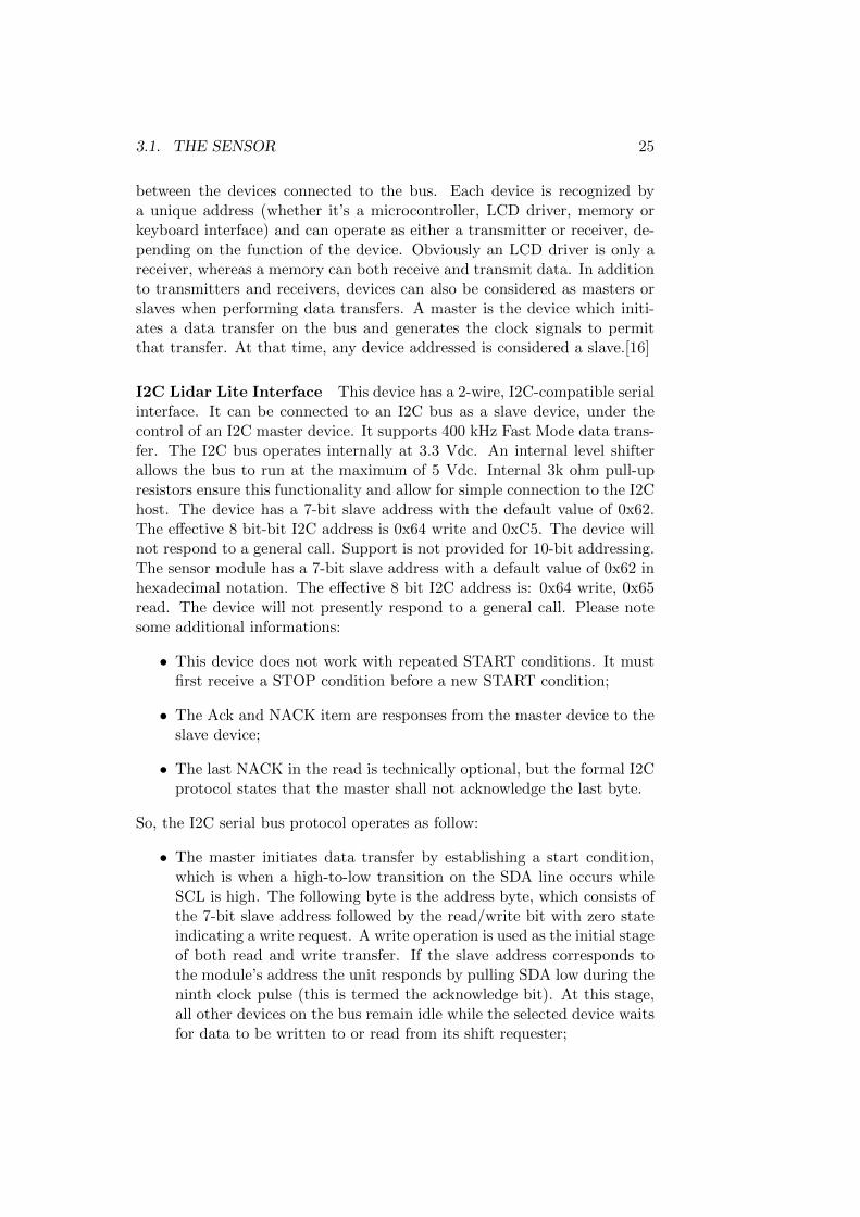
You can then use Atmel’s FLIP software (Windows) or the DFU programmer(Mac OS X and Linux) to load a new firmware. Or you can use the ISPheader with an external programmer (overwriting the DFU bootloader). Seethis user-contributed tutorial for more information.And then it’s possible to update and upload the code via USB thanks tothe appropriate software. It important to say that the arduino code is quitesimple and intuitive. To have an idea and understand how the basic ArduinoIDE environment is, please take a look at Fig. 3.2.
3.2.2 Connection Between Arduino and the Sensor
This example shows how to initialize, configure, and read distance from aLIDAR-Lite connected over the I2C interface. Connections:
• LIDAR-Lite 5 Vdc (red) to Arduino 5v
• LIDAR-Lite I2C SCL (green) to Arduino SCL
• LIDAR-Lite I2C SDA (blue) to Arduino SDA
• LIDAR-Lite Ground (black) to Arduino GND
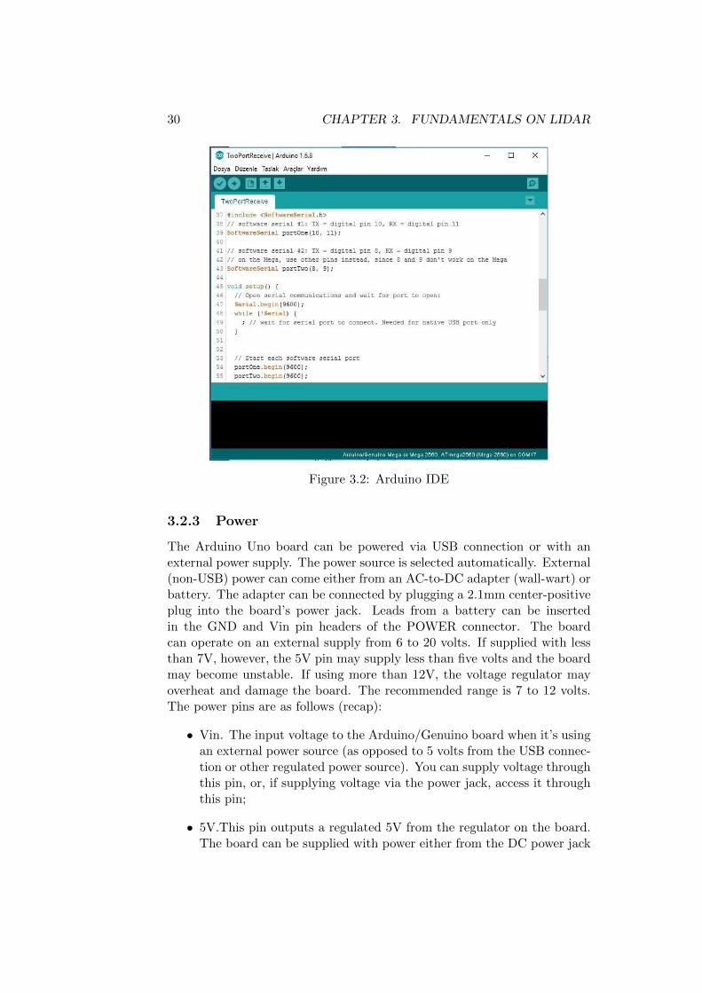
Somebody could raise the end and ask why it’s highly recommended to puta capacitor between the ground and 5V pin. The answer is quite immediateand easy: Capacitor is recommended to mitigate inrush current when deviceis enabled and, as said before, and as it’s possible to see in Fig. 3.3- 680uF capacitor (+) to Arduino 5v;- 680uF capacitor (-) to Arduino GND;
30 CHAPTER 3. FUNDAMENTALS ON LIDAR
Figure 3.2: Arduino IDE
3.2.3 Power
The Arduino Uno board can be powered via USB connection or with anexternal power supply. The power source is selected automatically. External(non-USB) power can come either from an AC-to-DC adapter (wall-wart) orbattery. The adapter can be connected by plugging a 2.1mm center-positiveplug into the board’s power jack. Leads from a battery can be insertedin the GND and Vin pin headers of the POWER connector. The boardcan operate on an external supply from 6 to 20 volts. If supplied with lessthan 7V, however, the 5V pin may supply less than five volts and the boardmay become unstable. If using more than 12V, the voltage regulator mayoverheat and damage the board. The recommended range is 7 to 12 volts.The power pins are as follows (recap):
• Vin. The input voltage to the Arduino/Genuino board when it’s usingan external power source (as opposed to 5 volts from the USB connec-tion or other regulated power source). You can supply voltage throughthis pin, or, if supplying voltage via the power jack, access it throughthis pin;
• 5V.This pin outputs a regulated 5V from the regulator on the board.The board can be supplied with power either from the DC power jack
3.2. ARDUINO 31
Figure 3.3: Aduino-LiDAR Connection
Item Description Notes
1 680 µF electrolytic capacitoryou must observe the correct polaritywhen installing the capacitor.
2 Power Ground (-) connection Black Wire3 I2C SDA connection Blu wire4 I2C SCL connection Green wire
5 5 Vdc power (+) connectionRed wireThe sensor operates at 4.75 through 5.5 Vdc,with a max. of 6 Vdc.
Table 3.6: Arduino-LiDAR Connection
(7 - 12V), the USB connector (5V), or the VIN pin of the board (7-12V). Supplying voltage via the 5V or 3.3V pins bypasses the regulator,and can damage your board;
• 3V3. A 3.3 volt supply generated by the on-board regulator. Maxi-mum current draw is 50 mA;
• GND. Ground pins;
• IOREF. This pin on the Arduino/Genuino board provides the voltagereference with which the microcontroller operates. A properly config-ured shield can read the IOREF pin voltage and select the appropriatepower source or enable voltage translators on the outputs to work withthe 5V or 3.3V.

32 CHAPTER 3. FUNDAMENTALS ON LIDAR
3.2.4 Input and Outputs
See the mapping between Arduino pins and ATmega328P ports. The map-ping for the Atmega8, 168, and 328 is identical.
Figure 3.4: Arduino ATMega Chipset
Each of the 14 digital pins on the Uno can be used as an input or output,using pinMode(),digitalWrite(), and digitalRead() functions. They operateat 5 volts. Each pin can provide or receive 20 mA as recommended operatingcondition and has an internal pull-up resistor (disconnected by default) of20-50kΩ. A maximum of 40mA is the value that must not be exceeded onany I/O pin to avoid permanent damage to the micro-controller. In addition,some pins have specialized functions:
• Serial: 0 (RX) and 1 (TX). Used to receive (RX) and transmit (TX)TTL serial data. These pins are connected to the corresponding pinsof the ATmega8U2 USB-to-TTL Serial chip;
• External Interrupts: 2 and 3. These pins can be configured to triggeran interrupt on a low value, a rising or falling edge, or a change invalue. See the attachInterrupt() function for details;
• PWM: 3, 5, 6, 9, 10, and 11. Provide 8-bit PWM output with theanalogWrite() function;
• SPI: 10 (SS), 11 (MOSI), 12 (MISO), 13 (SCK). These pins supportSPI communication using the SPI library;
• LED: 13. There is a built-in LED driven by digital pin 13. When thepin is HIGH value, the LED is on, when the pin is LOW, it’s off;
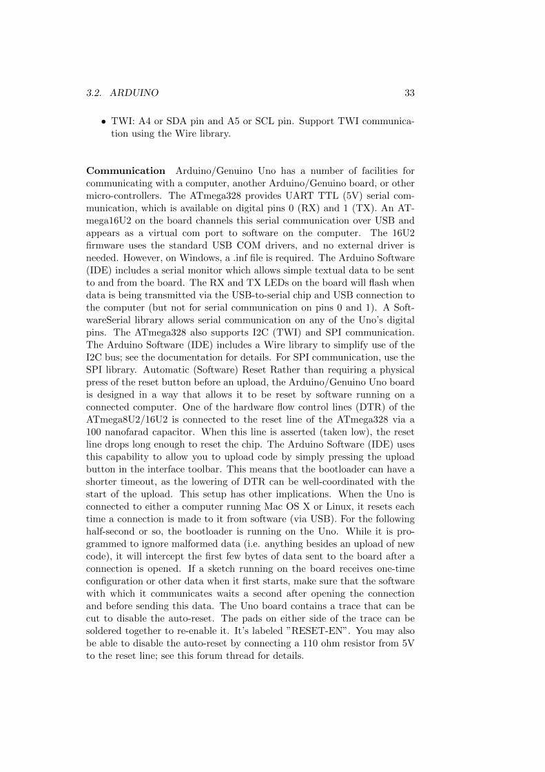
3.2. ARDUINO 33
• TWI: A4 or SDA pin and A5 or SCL pin. Support TWI communica-tion using the Wire library.
Communication Arduino/Genuino Uno has a number of facilities forcommunicating with a computer, another Arduino/Genuino board, or othermicro-controllers. The ATmega328 provides UART TTL (5V) serial com-munication, which is available on digital pins 0 (RX) and 1 (TX). An AT-mega16U2 on the board channels this serial communication over USB andappears as a virtual com port to software on the computer. The 16U2firmware uses the standard USB COM drivers, and no external driver isneeded. However, on Windows, a .inf file is required. The Arduino Software(IDE) includes a serial monitor which allows simple textual data to be sentto and from the board. The RX and TX LEDs on the board will flash whendata is being transmitted via the USB-to-serial chip and USB connection tothe computer (but not for serial communication on pins 0 and 1). A Soft-wareSerial library allows serial communication on any of the Uno’s digitalpins. The ATmega328 also supports I2C (TWI) and SPI communication.The Arduino Software (IDE) includes a Wire library to simplify use of theI2C bus; see the documentation for details. For SPI communication, use theSPI library. Automatic (Software) Reset Rather than requiring a physicalpress of the reset button before an upload, the Arduino/Genuino Uno boardis designed in a way that allows it to be reset by software running on aconnected computer. One of the hardware flow control lines (DTR) of theATmega8U2/16U2 is connected to the reset line of the ATmega328 via a100 nanofarad capacitor. When this line is asserted (taken low), the resetline drops long enough to reset the chip. The Arduino Software (IDE) usesthis capability to allow you to upload code by simply pressing the uploadbutton in the interface toolbar. This means that the bootloader can have ashorter timeout, as the lowering of DTR can be well-coordinated with thestart of the upload. This setup has other implications. When the Uno isconnected to either a computer running Mac OS X or Linux, it resets eachtime a connection is made to it from software (via USB). For the followinghalf-second or so, the bootloader is running on the Uno. While it is pro-grammed to ignore malformed data (i.e. anything besides an upload of newcode), it will intercept the first few bytes of data sent to the board after aconnection is opened. If a sketch running on the board receives one-timeconfiguration or other data when it first starts, make sure that the softwarewith which it communicates waits a second after opening the connectionand before sending this data. The Uno board contains a trace that can becut to disable the auto-reset. The pads on either side of the trace can besoldered together to re-enable it. It’s labeled ”RESET-EN”. You may alsobe able to disable the auto-reset by connecting a 110 ohm resistor from 5Vto the reset line; see this forum thread for details.

34 CHAPTER 3. FUNDAMENTALS ON LIDAR
3.3 Servo Motors
Servo motors are specially designed motors to be used in control applica-tions and robotics. They are used for precise position and speed control athigh torques. That’s why we thought that the servo could have been thebest choice for the LiDAR project. It consists of a suitable motor, positionsensor and a sophisticated controller. Servo motors can be characterizedaccording the motor controlled by servomechanism. Servo motors are avail-able in power ratings from fraction of watt up to few 100 watts. They arehaving high torque capabilities. The rotor of servo motor is made smallerin diameter and longer in length, so that it has low inertia. What Is Ser-vomechanism? Servomechanism is basically a closed-loop system Fig. 3.5,consisting of a controlled device, controller, output sensor and feedback sys-tem. The term servomechanism most probably applies to the systems whereposition and speed is to be controlled. Mechanical position of the shaft can
Figure 3.5: Servo Motor, scheme
be sensed by using a potentiometer, which is coupled with the motor shaftthrough gears. The current position of the shaft is converted into electricalsignal by the potentiometer, and then compared with the command inputsignal. In modern servo motors, electronic encoders or sensors are used tosense the position of the shaft. Command input is given according to therequired position of the shaft. If the feedback signal differs from the giveninput, an error signal is generated. This error signal is then amplified andapplied as the input to the motor, which causes the motor to rotate. Andwhen the shaft reaches the required position, error signal becomes zero, andhence the motor stays standstill holding the position.
3.3.1 How It Works
The simplicity of a servo is among the features that make them so reliable.The heart of a servo is a small direct current (DC) motor, similar to whatyou might find in an inexpensive toy. These motors run on electricity from

3.3. SERVO MOTORS 35
(a) Plastic Gears (b) Metal Gears
Figure 3.6: Stepper Gear examples
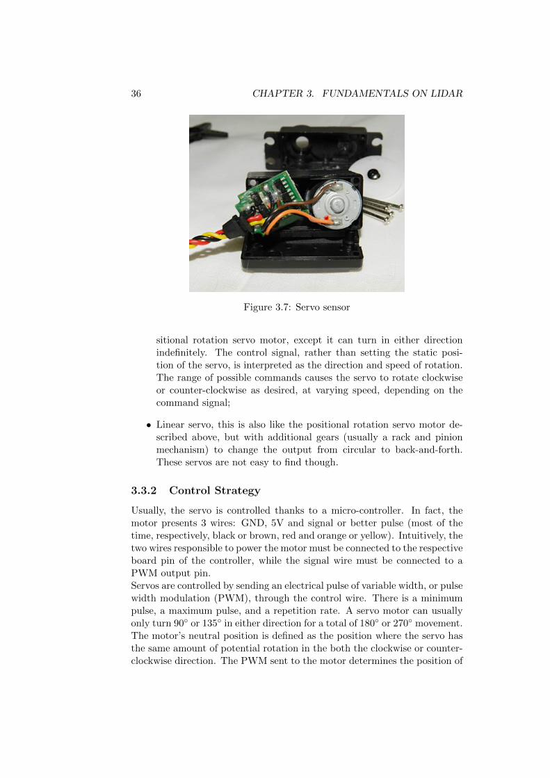
a battery or proper DC source and spin at high RPM (rotations per minute)but put out very low torque. An arrangement of gears takes the high speedof the motor and slows it down while at the same time increasing the torque.It’s common sense the basic law of physics: work = force × distance. Atiny electric motor does not have much torque, but it can spin really fast(small force, big distance). The gear design inside the servo case convertsthe output to a much slower rotation speed but with more torque (big force,little distance). Even though, the amount of actual work is the same. Gearsin an inexpensive servo motor are generally made of plastic to keep it lighterand less costly (see Fig. 3.6a). On a servo designed to provide more torquefor heavier work, the gears are made of metal (see Fig. 3.6b) and are harderto damage. With a small DC motor, you apply power from a battery, andthe motor spins. Unlike a simple DC motor, however, a servo’s spinningmotor shaft is slowed way down with gears. A positional sensor on thefinal gear is connected to a small circuit board (see Fig. 3.7). The sensortells this circuit board how far the servo output shaft has rotated. Theelectronic input signal from the computer feeds into that circuit board. Theelectronics on the circuit board decode the signals to determine how far theuser wants the servo to rotate. It then compares the desired position to theactual position and decides which direction to rotate the shaft so it gets tothe desired position. That is what makes servo motors so useful: once youtell them what you want done, they do the job without your help. Thisautomatic seeking behaviour of servo motors makes them perfect for manyrobotic applications.A lot of different kinds of servo motors are these days available:
• Positional rotation servo, this is the most common type of servo mo-tor. The output shaft rotates in about 90 degrees, 180 degrees or 270degrees. It has physical stops placed in the gear mechanism to preventturning beyond these limits to protect the rotational sensor;
• Continuous rotation servo, this is quite similar to the common po-
36 CHAPTER 3. FUNDAMENTALS ON LIDAR
Figure 3.7: Servo sensor
sitional rotation servo motor, except it can turn in either directionindefinitely. The control signal, rather than setting the static posi-tion of the servo, is interpreted as the direction and speed of rotation.The range of possible commands causes the servo to rotate clockwiseor counter-clockwise as desired, at varying speed, depending on thecommand signal;
• Linear servo, this is also like the positional rotation servo motor de-scribed above, but with additional gears (usually a rack and pinionmechanism) to change the output from circular to back-and-forth.These servos are not easy to find though.
3.3.2 Control Strategy
Usually, the servo is controlled thanks to a micro-controller. In fact, themotor presents 3 wires: GND, 5V and signal or better pulse (most of thetime, respectively, black or brown, red and orange or yellow). Intuitively, thetwo wires responsible to power the motor must be connected to the respectiveboard pin of the controller, while the signal wire must be connected to aPWM output pin.Servos are controlled by sending an electrical pulse of variable width, or pulsewidth modulation (PWM), through the control wire. There is a minimumpulse, a maximum pulse, and a repetition rate. A servo motor can usuallyonly turn 90 or 135 in either direction for a total of 180 or 270 movement.The motor’s neutral position is defined as the position where the servo hasthe same amount of potential rotation in the both the clockwise or counter-clockwise direction. The PWM sent to the motor determines the position of
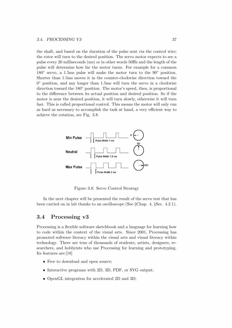
3.4. PROCESSING V3 37
the shaft, and based on the duration of the pulse sent via the control wire;the rotor will turn to the desired position. The servo motor expects to see apulse every 20 milliseconds (ms) or in other words 50Hz and the length of thepulse will determine how far the motor turns. For example for a common180 servo, a 1.5ms pulse will make the motor turn to the 90 position.Shorter than 1.5ms moves it in the counter-clockwise direction toward the0 position, and any longer than 1.5ms will turn the servo in a clockwisedirection toward the 180 position. The motor’s speed, then, is proportionalto the difference between its actual position and desired position. So if themotor is near the desired position, it will turn slowly, otherwise it will turnfast. This is called proportional control. This means the motor will only runas hard as necessary to accomplish the task at hand, a very efficient way toachieve the rotation, see Fig. 3.8.
Figure 3.8: Servo Control Strategy
In the next chapter will be presented the result of the servo test that hasbeen carried on in lab thanks to an oscilloscope (See §Chap. 4, §Sec. 4.2.1).
3.4 Processing v3
Processing is a flexible software sketchbook and a language for learning howto code within the context of the visual arts. Since 2001, Processing haspromoted software literacy within the visual arts and visual literacy withintechnology. There are tens of thousands of students, artists, designers, re-searchers, and hobbyists who use Processing for learning and prototyping.Its features are:[18]
• Free to download and open source;
• Interactive programs with 2D, 3D, PDF, or SVG output;
• OpenGL integration for accelerated 2D and 3D;
38 CHAPTER 3. FUNDAMENTALS ON LIDAR
• For GNU/Linux, Mac OS X, Windows, Android, and ARM;
• Over 100 libraries extend the core software;
• Well documented, with many books available;
Processing is an open-source graphical library and integrated developmentenvironment (IDE) / playground built for the electronic arts, new me-dia art, and visual design communities with the purpose of teaching non-programmers the fundamentals of computer programming in a visual con-text. Processing uses the Java language, with additional simplifications suchas additional classes and aliased mathematical functions and operations. Aswell as this, it also has a graphical user interface for simplyfing the com-pilation and execution stage. The Processing language and IDE were theprecursor to numerous other projects, notably Arduino, Wiring and P5.js.Processing includes a sketchbook, a minimal alternative to an integrateddevelopment environment (IDE)(See Fig. 3.9) for organizing projects.[19]
Every Processing sketch is actually a subclass of the PApplet Java class(formerly a subclass of Java’s built-in Applet) which implements most ofthe Processing language’s features.[20] When programming in Processing,all additional classes defined will be treated as inner classes when the codeis translated into pure Java before compiling.[21] This means that the useof static variables and methods in classes is prohibited unless Processing isexplicitly told to code in pure Java mode. Processing also allows for usersto create their own classes within the PApplet sketch. This allows for com-plex data types that can include any number of arguments and avoids thelimitations of solely using standard data types such as: int (integer), char(character), float (real number), and color (RGB, RGBA, hex). Processingrelates software concepts to principles of visual form, motion, and interac-tion. It integrates a programming language, development environment, andteaching methodology into a unified system. The Processing language is atext programming language specifically designed to generate and modify im-ages. Processing strives to achieve a balance between clarity and advancedfeatures. Beginners can write their own programs after only a few min-utes of instruction, but more advanced users can employ and write librarieswith additional functions. The system facilitates teaching many computergraphics and interaction techniques including vector/raster drawing, imageprocessing, color models, mouse and keyboard events, network communica-tion, and object-oriented programming. Libraries easily extend Processing’sability to generate sound, send/receive data in diverse formats, and to im-port/export 2D and 3D file formats.[22]So, thanks to the concepts presented in this chapter it will be possible toexplain how the first LiDAR platform has been built.
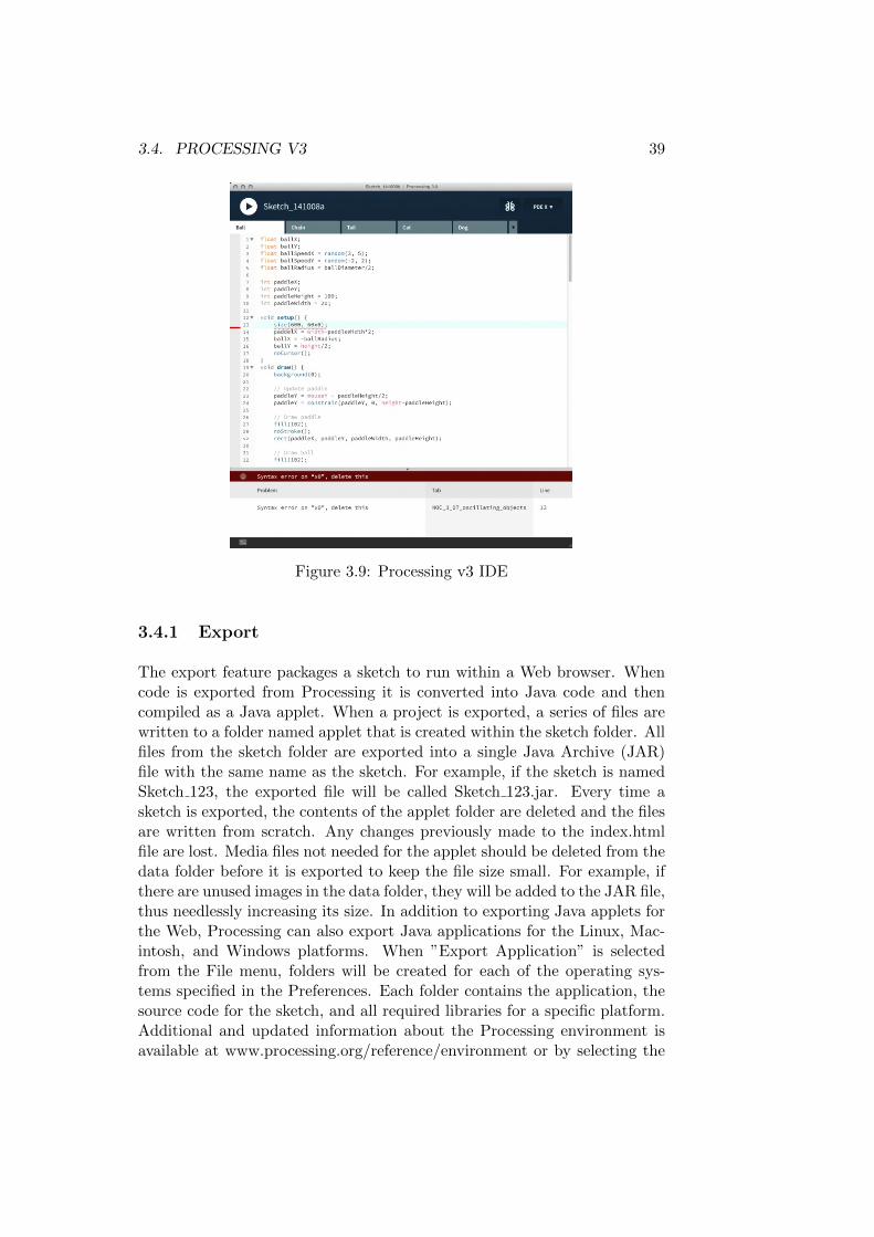
3.4. PROCESSING V3 39
Figure 3.9: Processing v3 IDE
3.4.1 Export
The export feature packages a sketch to run within a Web browser. Whencode is exported from Processing it is converted into Java code and thencompiled as a Java applet. When a project is exported, a series of files arewritten to a folder named applet that is created within the sketch folder. Allfiles from the sketch folder are exported into a single Java Archive (JAR)file with the same name as the sketch. For example, if the sketch is namedSketch 123, the exported file will be called Sketch 123.jar. Every time asketch is exported, the contents of the applet folder are deleted and the filesare written from scratch. Any changes previously made to the index.htmlfile are lost. Media files not needed for the applet should be deleted from thedata folder before it is exported to keep the file size small. For example, ifthere are unused images in the data folder, they will be added to the JAR file,thus needlessly increasing its size. In addition to exporting Java applets forthe Web, Processing can also export Java applications for the Linux, Mac-intosh, and Windows platforms. When ”Export Application” is selectedfrom the File menu, folders will be created for each of the operating sys-tems specified in the Preferences. Each folder contains the application, thesource code for the sketch, and all required libraries for a specific platform.Additional and updated information about the Processing environment isavailable at www.processing.org/reference/environment or by selecting the

40 CHAPTER 3. FUNDAMENTALS ON LIDAR
”Environment” item from the Help menu of the Processing application.[22]
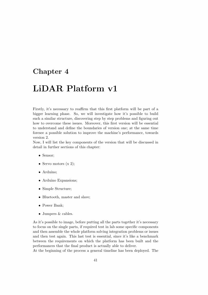
Chapter 4
LiDAR Platform v1
Firstly, it’s necessary to reaffirm that this first platform will be part of abigger learning phase. So, we will investigate how it’s possible to buildsuch a similar structure, discovering step by step problems and figuring outhow to overcome these issues. Moreover, this first version will be essentialto understand and define the boundaries of version one; at the same timeforesee a possible solution to improve the machine’s performance, towardsversion 2.Now, I will list the key components of the version that will be discussed indetail in further sections of this chapter:
• Sensor;
• Servo motors (x 2);
• Arduino;
• Arduino Expansions;
• Simple Structure;
• Bluetooth, master and slave;
• Power Bank;
• Jumpers & cables.
As it’s possible to image, before putting all the parts together it’s necessaryto focus on the single parts, if required test in lab some specific componentsand then assemble the whole platform solving integration problems or issuesand then test again. This last test is essential, since it’s like a benchmarkbetween the requirements on which the platform has been built and theperformances that the final product is actually able to deliver.At the beginning of the process a general timeline has been deployed. The
41
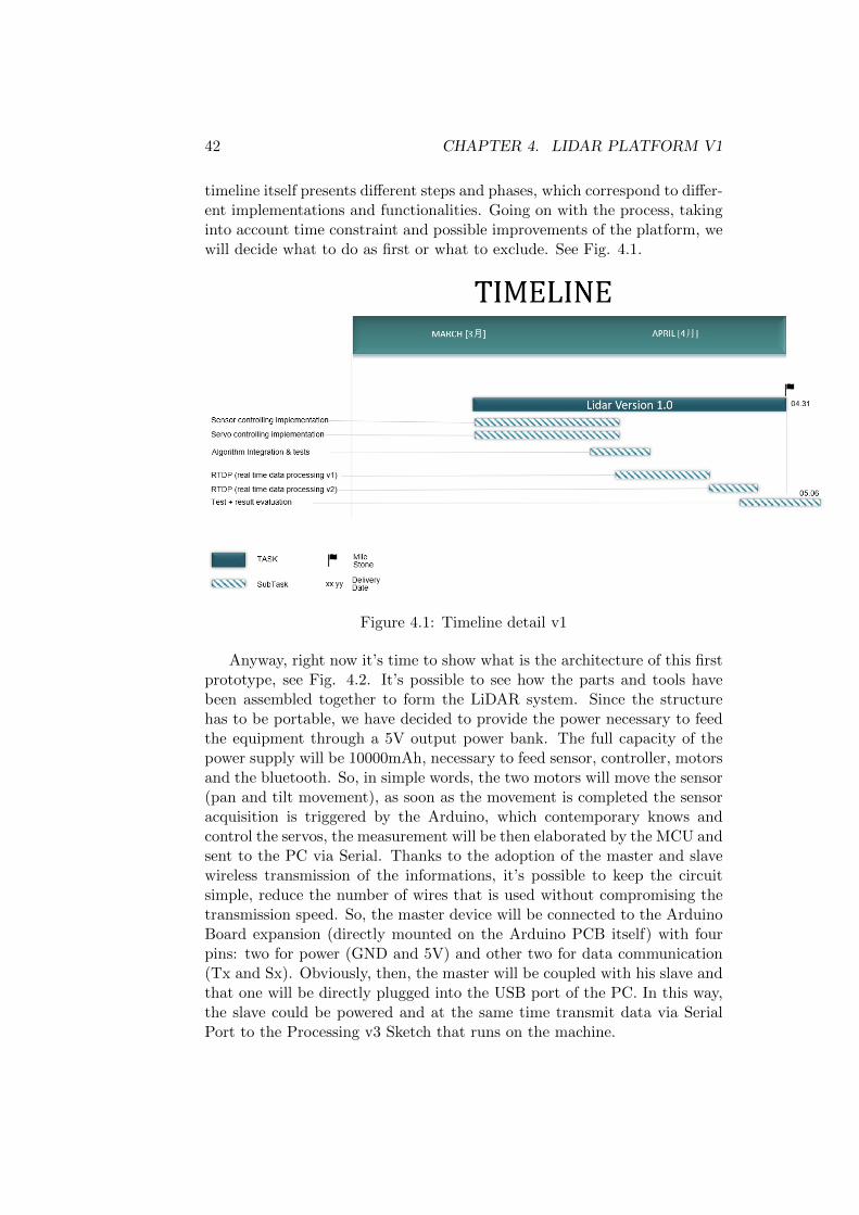
42 CHAPTER 4. LIDAR PLATFORM V1
timeline itself presents different steps and phases, which correspond to differ-ent implementations and functionalities. Going on with the process, takinginto account time constraint and possible improvements of the platform, wewill decide what to do as first or what to exclude. See Fig. 4.1.
Figure 4.1: Timeline detail v1
Anyway, right now it’s time to show what is the architecture of this firstprototype, see Fig. 4.2. It’s possible to see how the parts and tools havebeen assembled together to form the LiDAR system. Since the structurehas to be portable, we have decided to provide the power necessary to feedthe equipment through a 5V output power bank. The full capacity of thepower supply will be 10000mAh, necessary to feed sensor, controller, motorsand the bluetooth. So, in simple words, the two motors will move the sensor(pan and tilt movement), as soon as the movement is completed the sensoracquisition is triggered by the Arduino, which contemporary knows andcontrol the servos, the measurement will be then elaborated by the MCU andsent to the PC via Serial. Thanks to the adoption of the master and slavewireless transmission of the informations, it’s possible to keep the circuitsimple, reduce the number of wires that is used without compromising thetransmission speed. So, the master device will be connected to the ArduinoBoard expansion (directly mounted on the Arduino PCB itself) with fourpins: two for power (GND and 5V) and other two for data communication(Tx and Sx). Obviously, then, the master will be coupled with his slave andthat one will be directly plugged into the USB port of the PC. In this way,the slave could be powered and at the same time transmit data via SerialPort to the Processing v3 Sketch that runs on the machine.
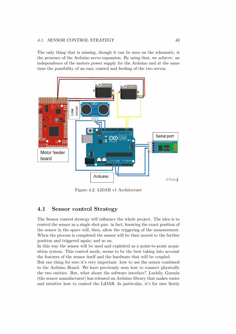
4.1. SENSOR CONTROL STRATEGY 43
The only thing that is missing, though it can be seen on the schematic, isthe presence of the Arduino servo expansion. By using that, we achieve: anindependence of the motors power supply for the Arduino and at the sametime the possibility of an easy control and feeding of the two servos.
Figure 4.2: LiDAR v1 Architecture
4.1 Sensor control Strategy
The Sensor control strategy will influence the whole project. The idea is tocontrol the sensor as a single shot gun: in fact, knowing the exact position ofthe sensor in the space will, then, allow the triggering of the measurement.When the process is completed the sensor will be then moved to the furtherposition and triggered again; and so on.In this way the sensor will be used and exploited as a point-to-point acqui-sition system. This control mode, seems to be the best taking into accountthe features of the sensor itself and the hardware that will be coupled.But one thing for sure it’s very important: how to use the sensor combinedto the Arduino Board. We have previously seen how to connect physicallythe two entities. But, what about the software interface? Luckily, Garmin(the sensor manufacturer) has released an Arduino library that makes easierand intuitive how to control the LiDAR. In particular, it’s for sure firstly

44 CHAPTER 4. LIDAR PLATFORM V1
necessary to install the library in the Arduino library folder. Once that thisstep has been done, the sensor can be easily controlled and trigger, as saidbefore.Firstly, it’s mandatory to define the LiDAR OBJECT with a proper syntax.Then, it’s necessary to initiate the communication via I2C (the transmis-sion mode we have chosen). Then, with a single command is possible totrigger the sensor and capture the measurement. Anyway, the sensor canoperate in different modes and with two levels of accuracy. Obviously, thedeal it’s a compromise between speed and reliability of the data gatheredby the sensor. The following listed code explains basically how to operatethe sensor:
1 /∗−−−−−−−−−−−−−−−−−−−−−−−−−−−−−−−−−−−−−−−−−−−−−2 This example shows how to i n i t i a l i z e , con f i gure ,3 and read d i s t ance from a LIDAR−Li t e connected over I2C
i n t e r f a c e .4
5 Connections :6 LIDAR−Li t e 5 Vdc ( red ) to Arduino 5v7 LIDAR−Li t e I2C SCL ( green ) to Arduino SCL8 LIDAR−Li t e I2C SDA ( blue ) to Arduino SDA9 LIDAR−Li t e Ground ( black ) to Arduino GND
10
11 ( Capacitor recommended to mi t i ga t e inrush cur rent when dev i cei s enabled )
12 680uF c a p a c i t o r (+) to Arduino 5v13 680uF c a p a c i t o r (−) to Arduino GND14 −−−−−−−−−−−−−−−−−−−−−−−−−−−−−−−−−−−−−−−−−−−−−∗/15 #inc lude <Wire . h> // Standard Library16 #inc lude <LIDARLite . h> // LiDAR ’ s Library17
18 LIDARLite myLidarLite ; // LiDAR OBJECT DEFINITION19
20 void setup ( )21 22 S e r i a l . begin (115200) ; // I n i t i a l i z e s e r i a l connect ion to
d i s p l ay d i s t ance r ead ings23 /∗24 begin ( i n t con f i gu ra t i on , bool f a s t i 2 c , char l i d a r l i t e A d d r e s s )25 −> S t a r t s the s enso r and I2C .26
27 Parameters28 −−−−−−−−−−−−−−−−−−−−−−−−−−−−−−−−−−−−−−−−−−−−−29 c o n f i g u r a t i o n : Defau l t 0 .30 S e l e c t s one o f s e v e r a l p r e s e t c o n f i g u r a t i o n s .31 f a s t i 2 c : Defau l t 100 kHz . I2C base f requency . ( I f t rue I2C
frequency i s s e t to 400kHz) ∗/32 myLidarLite . begin (0 , t rue ) ; // Set c o n f i g u r a t i o n to d e f a u l t
and I2C to 400 kHz33 /∗ c o n f i g u r e ( i n t con f i gu ra t i on , char l i d a r l i t e A d d r e s s )34 S e l e c t s one o f s e v e r a l p r e s e t c o n f i g u r a t i o n s .35 Parameters

4.1. SENSOR CONTROL STRATEGY 45
36 −−−−−−−−−−−−−−−−−−−−−−−−−−−−−−−−−−−−−−−−−−−−−37 c o n f i g u r a t i o n : Defau l t 0 .38 0 : Defau l t mode , balanced performance .39 1 : Short range , high speed . Uses 0x1d maximum a c q u i s i t i o n
count .40 2 : Defau l t range , h igher speed shor t range . Turns on quick
te rminat ion d e t e c t i o n f o r f a s t e r measurements at shor t range (with decreased accuracy ) .
41 3 : Maximum range . Uses 0 x f f maximum a c q u i s i t i o n count .42 4 : High s e n s i t i v i t y d e t e c t i o n . Overr ides d e f a u l t v a l i d
measurement d e t e c t i o n algorithm , and uses a th r e sho ld valuef o r high s e n s i t i v i t y and no i s e .
43 5 : Low s e n s i t i v i t y d e t e c t i o n . Overr ides d e f a u l t v a l i dmeasurement d e t e c t i o n algorithm , and uses a th r e sho ld valuef o r low s e n s i t i v i t y and no i s e . ∗/
44 myLidarLite . c o n f i g u r e (0 ) ; // Change t h i s number to t ry outa l t e r n a t e c o n f i g u r a t i o n s
45 46 void loop ( )47 48 /∗ d i s t ance ( bool b ia sCor rec t i on , char l i d a r l i t e A d d r e s s )49 Take a d i s t ance measurement and read the r e s u l t .50 Parameters51 −−−−−−−−−−−−−−−−−−−−−−−−−−−−−−−−−−−−−−−−−−−−−52 b ia sCor r e c t i on : Defau l t t rue . Take a c q u i s i t i o n with r e c e i v e r
b i a s c o r r e c t i o n . I f s e t to f a l s e measurements w i l l be f a s t e r .Rece iver b i a s c o r r e c t i o n must be performed p e r i o d i c a l l y . ( e .
g . 1 out o f every 100 \ r ead ings ) . ∗/53
54 // Take a measurement with r e c e i v e r b i a s c o r r e c t i o n and pr in tto s e r i a l t e rmina l
55 S e r i a l . p r i n t l n ( myLidarLite . d i s t ance ( ) ) ;56
57 // Take 99 measurements without r e c e i v e r b i a s c o r r e c t i o n andpr in t to s e r i a l t e rmina l
58 f o r ( i n t i = 0 ; i < 99 ; i++)59 60 S e r i a l . p r i n t l n ( myLidarLite . d i s t ance ( f a l s e ) ) ;61 62
Listing 4.1: Code Listing-sensor acquisition
Taking a look at the code listing 4.1; it’s possible to see that on:
• Line 18, LiDAR Object has been defined;
• Line 32, I2C communication starts, with default settings (value = 0)and speed set to 400kHz (true);
• Line 44, set LiDAR operational mode (value = 0, balanced perfor-mances);
• Line 55, acquisition trigger (no bias correction). It means that themeasure is faster but not super accurate; as we have said the measure
46 CHAPTER 4. LIDAR PLATFORM V1
is a compromise between acquisition speed and accuracy. So it’s rec-ommended to re-calibrate the sensor every 100 points, to get a moreprecise distance value.
4.2 Servo control Strategy
The servo control strategy it’s pretty straight forward. Again, Arduino helpsus since the servo library it’s available. As we have said, standard servosallow the shaft to be positioned at various angles, usually between 0 and180 degrees. The Servo library supports up to 12 motors on most Arduinoboards and 48 on the Arduino Mega. Once, the servo is powered and thepulse wire is connected to a PWM Arduino output pin, it’s necessary todeclare two servo entities (pan and tilt motor, motor x and motor y). Then,the game is quite simple: in fact it’s necessary to remember that the servo’sshaft can assume each position between 0 and 180. To change the shaft’sposition it’s just needed to use the library’s instruction write. While, if wewant to know the exact position of the servo we can use the instruction read.Both, read and write, are used as attributes or methods applied to the servoentities.
Servo Trajectory At this point it will be briefly discussed an hot topic,that will be treated for sure with a deeper focus in following sections. Thefinal density of the point cloud1 is linked for sure to the reliability of thesensor and its capability to trigger and gather distances in the smallestpossible period of time. But, assuming that the sensor is fast enough, as itactually is, the main driver that determines the density of the point cloudis the minimum step that the servo can execute. Taking a look on theinternet and LiDAR commercial products, it’s noticeable that extremelydetailed point clouds reach, at least, densities around 1 or 2 million points(over a 3D sapace which is roughly 180 × 90, in other words half of asemi-sphere). For this first prototype, though, the density is absolutelylower, around 200000 points. This comes from a very simple mathematicalcalculation, considering the smallest servo’s movement equal to 1 degreeand a scanned 3D space which is actually close to half of a semi-sphere.At this point, we don’t know yet if this density is enough to distinguish,at least roughly, obstacles and scanned objects. In the final phase of thedevelopment step this aspect will be checked and discussed: if the resultit’s not considered acceptable, the version2 will be completely focused on a
1A point cloud is a set of data points in space. Point clouds are generally produced by3D scanners, which measure a large number of points on the external surfaces of objectsaround them. As the output of 3D scanning processes, point clouds are used for manypurposes, including to create 3D CAD models for manufactured parts, for metrology andquality inspection, and for a multitude of visualization, animation, rendering and masscustomization applications.
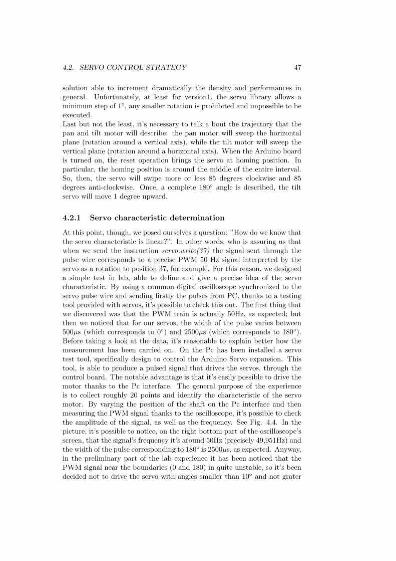
4.2. SERVO CONTROL STRATEGY 47
solution able to increment dramatically the density and performances ingeneral. Unfortunately, at least for version1, the servo library allows aminimum step of 1, any smaller rotation is prohibited and impossible to beexecuted.Last but not the least, it’s necessary to talk a bout the trajectory that thepan and tilt motor will describe: the pan motor will sweep the horizontalplane (rotation around a vertical axis), while the tilt motor will sweep thevertical plane (rotation around a horizontal axis). When the Arduino boardis turned on, the reset operation brings the servo at homing position. Inparticular, the homing position is around the middle of the entire interval.So, then, the servo will swipe more or less 85 degrees clockwise and 85degrees anti-clockwise. Once, a complete 180 angle is described, the tiltservo will move 1 degree upward.
4.2.1 Servo characteristic determination
At this point, though, we posed ourselves a question: ”How do we know thatthe servo characteristic is linear?”. In other words, who is assuring us thatwhen we send the instruction servo.write(37) the signal sent through thepulse wire corresponds to a precise PWM 50 Hz signal interpreted by theservo as a rotation to position 37, for example. For this reason, we designeda simple test in lab, able to define and give a precise idea of the servocharacteristic. By using a common digital oscilloscope synchronized to theservo pulse wire and sending firstly the pulses from PC, thanks to a testingtool provided with servos, it’s possible to check this out. The first thing thatwe discovered was that the PWM train is actually 50Hz, as expected; butthen we noticed that for our servos, the width of the pulse varies between500µs (which corresponds to 0) and 2500µs (which corresponds to 180).Before taking a look at the data, it’s reasonable to explain better how themeasurement has been carried on. On the Pc has been installed a servotest tool, specifically design to control the Arduino Servo expansion. Thistool, is able to produce a pulsed signal that drives the servos, through thecontrol board. The notable advantage is that it’s easily possible to drive themotor thanks to the Pc interface. The general purpose of the experienceis to collect roughly 20 points and identify the characteristic of the servomotor. By varying the position of the shaft on the Pc interface and thenmeasuring the PWM signal thanks to the oscilloscope, it’s possible to checkthe amplitude of the signal, as well as the frequency. See Fig. 4.4. In thepicture, it’s possible to notice, on the right bottom part of the oscilloscope’sscreen, that the signal’s frequency it’s around 50Hz (precisely 49,951Hz) andthe width of the pulse corresponding to 180 is 2500µs, as expected. Anyway,in the preliminary part of the lab experience it has been noticed that thePWM signal near the boundaries (0 and 180) in quite unstable, so it’s beendecided not to drive the servo with angles smaller than 10 and not grater

48 CHAPTER 4. LIDAR PLATFORM V1
Figure 4.3: Servo lab test 1
than 170, since there’s no linearity in this portion of the characteristic.So, then, the characteristic has been drawn testing 20 positions, especiallyclose to the upper and lower limit of the servo previously fixed. Taking alook at Tab. 4.1 and to Fig 4.5 it’s possible to see clearly that the servocharacteristic is pretty linear, or at least it’s quite possible to consider itlinear. This was the result we were looking for, considering the fact thatthe resolution of the point cloud and the accuracy of the point positioningis strictly dependent on the servos.
4.3 Data Elaboration and Transmission
Right now, this chapter has explained the main mechanism around the sen-sor acquisition and servo controlling. The output of the LiDAR sensor mea-surement is a distance, associated to two angular positions, respectively re-lated to the two motors. It’s intuitive that the sensor describes a trajectorythat moves on a semi-sphere. At the same time, though, the final repre-sentation that we want is a three dimensional picture based on a Cartesiancoordinate system.
T(ρ,θ,φ) ⇒ T(x,y,z) (4.1)

4.3. DATA ELABORATION AND TRANSMISSION 49
Degrees Pulse Amplitude (µs)
10 60012 640,814 660,416 680,518 700,320 720,522 740,424 760,226 780,528 800,530 820,332 84090 1502150 2161151 2180153 2200155 2220157 2241160 2280163 2030165 2320169 2360170 2400
Table 4.1: Servo Characteristic
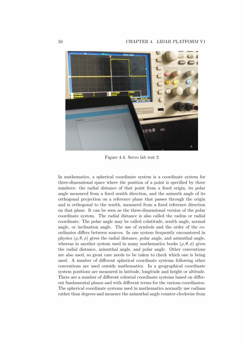
50 CHAPTER 4. LIDAR PLATFORM V1
Figure 4.4: Servo lab test 2
In mathematics, a spherical coordinate system is a coordinate system forthree-dimensional space where the position of a point is specified by threenumbers: the radial distance of that point from a fixed origin, its polarangle measured from a fixed zenith direction, and the azimuth angle of itsorthogonal projection on a reference plane that passes through the originand is orthogonal to the zenith, measured from a fixed reference directionon that plane. It can be seen as the three-dimensional version of the polarcoordinate system. The radial distance is also called the radius or radialcoordinate. The polar angle may be called colatitude, zenith angle, normalangle, or inclination angle. The use of symbols and the order of the co-ordinates differs between sources. In one system frequently encountered inphysics (ρ, θ, φ) gives the radial distance, polar angle, and azimuthal angle,whereas in another system used in many mathematics books (ρ, θ, φ) givesthe radial distance, azimuthal angle, and polar angle. Other conventionsare also used, so great care needs to be taken to check which one is beingused. A number of different spherical coordinate systems following otherconventions are used outside mathematics. In a geographical coordinatesystem positions are measured in latitude, longitude and height or altitude.There are a number of different celestial coordinate systems based on differ-ent fundamental planes and with different terms for the various coordinates.The spherical coordinate systems used in mathematics normally use radiansrather than degrees and measure the azimuthal angle counter-clockwise from

4.3. DATA ELABORATION AND TRANSMISSION 51
Figure 4.5: Servo Characteristic, graph
the x-axis to the y-axis rather than clockwise from north (0) to east (90)like the horizontal coordinate system. The polar angle is often replacedby the elevation angle measured from the reference plane. Elevation angleof zero is at the horizon. The spherical coordinate system generalizes thetwo-dimensional polar coordinate system. It can also be extended to higher-dimensional spaces and is then referred to as a hyper-spherical coordinatesystem.
Spherical coordinates determine the position of a point in three-dimensionalspace based on the distance ρ from the origin and two angles θ and φ. Thefollowing graphics (See Fig. 4.6) may help to understand spherical coordi-nates better. On this page, we derive the relationship between spherical andCartesian coordinates.
Relationship between spherical and Cartesian coordinates Spher-ical coordinates are defined as indicated in the following figure, which il-lustrates the spherical coordinates of the point P. The coordinate ρ is thedistance from P to the origin. If the point Q is the projection of P tothe xy-plane, then θ is the angle between the positive x-axis and the linesegment from the origin to Q. Lastly, φ is the angle between the positivez-axis and the line segment from the origin to P. We can calculate therelationship between the Cartesian coordinates (x, y, z) of the point P andits spherical coordinates (ρ, θ, φ) using trigonometry. The pink triangle (SeeFig. 4.7) is the right triangle whose vertices are the origin, the point P, andits projection onto the z-axis. As the length of the hypotenuse is ρ and φ
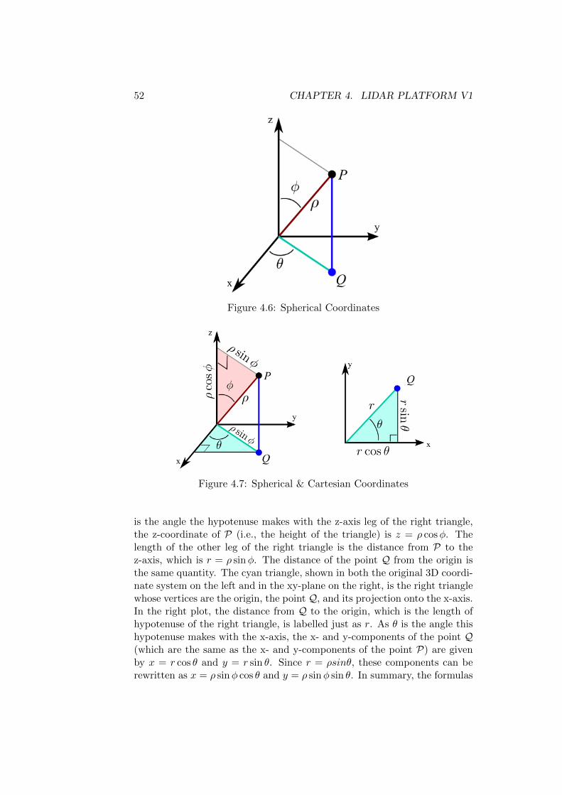
52 CHAPTER 4. LIDAR PLATFORM V1
Figure 4.6: Spherical Coordinates
Figure 4.7: Spherical & Cartesian Coordinates
is the angle the hypotenuse makes with the z-axis leg of the right triangle,the z-coordinate of P (i.e., the height of the triangle) is z = ρ cosφ. Thelength of the other leg of the right triangle is the distance from P to thez-axis, which is r = ρ sinφ. The distance of the point Q from the origin isthe same quantity. The cyan triangle, shown in both the original 3D coordi-nate system on the left and in the xy-plane on the right, is the right trianglewhose vertices are the origin, the point Q, and its projection onto the x-axis.In the right plot, the distance from Q to the origin, which is the length ofhypotenuse of the right triangle, is labelled just as r. As θ is the angle thishypotenuse makes with the x-axis, the x- and y-components of the point Q(which are the same as the x- and y-components of the point P) are givenby x = r cos θ and y = r sin θ. Since r = ρsinθ, these components can berewritten as x = ρ sinφ cos θ and y = ρ sinφ sin θ. In summary, the formulas

4.4. DATA PROCESSING, VISUALIZATION AND RESULTS 53
for Cartesian coordinates in terms of spherical coordinates are:
x = ρ sinφ cos θ
y = ρ sinφ sin θ
z = ρ cos θ
So, once the sensor has revealed the distance, there are some lines in theArduino code that operates the transformation and then print a string with(x, y, z) on the serial port. This operation it’s quite easy thanks to theinstruction println. It is as well possible to print the data to file, but actuallywe preferred to transmit the data via Serial: in this way it’s immediate areal time elaboration.
4.4 Data Processing, Visualization and Results
Since the scanning process has been totally explained, now it’s the visual-ization turn. Once, the data has been collected, then there’s the need toshow them and create a virtual environment which let us appreciate theshapes of scanned objects. Moreover, as we have chosen, we want it to bereal time, which means that the scanning process and visualization processare contemporary.In other words, as previously hinted in §Chap. 3, §Sec. 3.4, a processingsketch running on the Pc will show the point cloud. The sketch should:
• Read real time the Serial Port;
• Store temporarily the data in a matrix;
• Plot the data without delays;
• Assign a proper color to each point;
• Offer a proper navigation system;
• Allow to save data.
As a matter of facts, the Arduino output is (x, y, z) coordinates, so theprocessing v3 sketch accepts (x, y, z) data as input. The big deal is to setthe correct Serial Port speed, synchronized to the Arduino transmissionbaud rate.
1 // This sketch accept s XYZ coo rd ina t e s from Arduino LIDARscanner and d i s p l a y s them g r a p h i c a l l y as a 3D point c loudthat you can pan , zoom , and r o t a t e us ing keyboard .
2
3 import p r o c e s s i n g . s e r i a l . ∗ ; // S e r i a l Port Java l i b r a r y4 import java . i o . F i l eWr i t e r ; // l i b r a r i e s nece s sa ry to export
f i l e
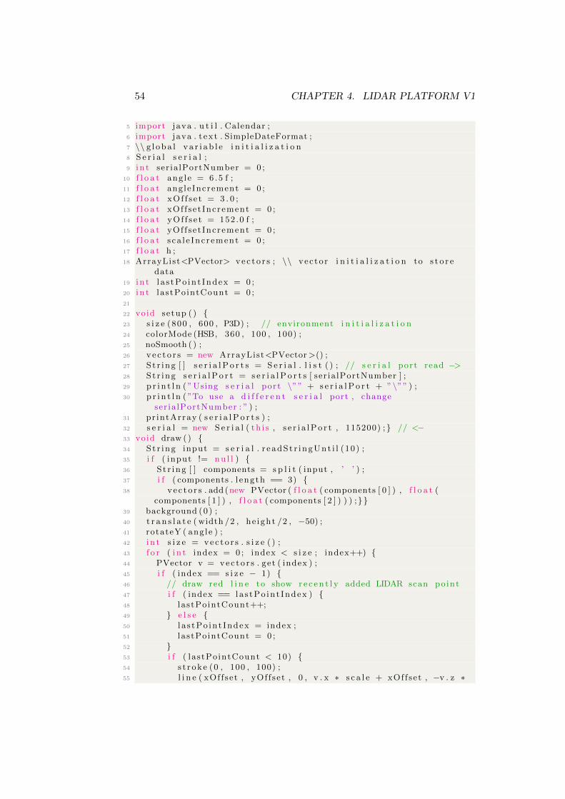
54 CHAPTER 4. LIDAR PLATFORM V1
5 import java . u t i l . Calendar ;6 import java . t ex t . SimpleDateFormat ;7 \\ g l o b a l v a r i a b l e i n i t i a l i z a t i o n8 S e r i a l s e r i a l ;9 i n t ser ia lPortNumber = 0 ;
10 f l o a t ang le = 6 .5 f ;11 f l o a t angleIncrement = 0 ;12 f l o a t xOf f s e t = 3 . 0 ;13 f l o a t xOf f set Increment = 0 ;14 f l o a t yOf f s e t = 152 .0 f ;15 f l o a t yOf f set Increment = 0 ;16 f l o a t s ca l e Inc rement = 0 ;17 f l o a t h ;18 ArrayList<PVector> ve c t o r s ; \\ vec to r i n i t i a l i z a t i o n to s t o r e
data19 i n t l a s tPo in t Index = 0 ;20 i n t lastPointCount = 0 ;21
22 void setup ( ) 23 s i z e (800 , 600 , P3D) ; // environment i n i t i a l i z a t i o n24 colorMode (HSB, 360 , 100 , 100) ;25 noSmooth ( ) ;26 ve c t o r s = new ArrayList<PVector >() ;27 St r ing [ ] s e r i a l P o r t s = S e r i a l . l i s t ( ) ; // s e r i a l port read −>28 St r ing s e r i a l P o r t = s e r i a l P o r t s [ ser ia lPortNumber ] ;29 p r i n t l n ( ”Using s e r i a l port \”” + s e r i a l P o r t + ”\”” ) ;30 p r i n t l n ( ”To use a d i f f e r e n t s e r i a l port , change
ser ia lPortNumber : ” ) ;31 pr intArray ( s e r i a l P o r t s ) ;32 s e r i a l = new S e r i a l ( th i s , s e r i a l P o r t , 115200) ; // <−33 void draw ( ) 34 St r ing input = s e r i a l . r e adSt r i ngUnt i l (10) ;35 i f ( input != n u l l ) 36 St r ing [ ] components = s p l i t ( input , ’ ’ ) ;37 i f ( components . l ength == 3) 38 ve c t o r s . add (new PVector ( f l o a t ( components [ 0 ] ) , f l o a t (
components [ 1 ] ) , f l o a t ( components [ 2 ] ) ) ) ;39 background (0) ;40 t r a n s l a t e ( width /2 , he ight /2 , −50) ;41 rotateY ( ang le ) ;42 i n t s i z e = ve c to r s . s i z e ( ) ;43 f o r ( i n t index = 0 ; index < s i z e ; index++) 44 PVector v = ve c to r s . get ( index ) ;45 i f ( index == s i z e − 1) 46 // draw red l i n e to show r e c e n t l y added LIDAR scan po int47 i f ( index == las tPo in t Index ) 48 lastPointCount++;49 e l s e 50 l a s tPo in t Index = index ;51 lastPointCount = 0 ;52 53 i f ( lastPointCount < 10) 54 s t r oke (0 , 100 , 100) ;55 l i n e ( xOf f set , yOf f set , 0 , v . x ∗ s c a l e + xOffset , −v . z ∗

4.4. DATA PROCESSING, VISUALIZATION AND RESULTS 55
s c a l e + yOffset , −v . y ∗ s c a l e ) ;56 h= s q r t ( v . x∗v . x+v . y∗v . y+v . z∗v . z ) ;57 s t r oke (360−(h ∗0 . 4 ) , 100 , 100) ;58 point ( v . x ∗ s c a l e + xOffset , −v . z ∗ s c a l e + yOffset , −v . y ∗
s c a l e ) ;59 ang le += angleIncrement ;60 xOf f s e t += xOff set Increment ;61 yOf f s e t += yOff set Increment ;62 s c a l e += sca l e Inc rement ;63 void keyPressed ( ) 64 i f ( key == ’ q ’ ) 65 // zoom in66 s ca l e Inc rement = 0.02 f ;67 e l s e i f ( key == ’ z ’ ) 68 // zoom out69 s ca l e Inc rement = −0.02 f ;70 e l s e i f ( key ==’p ’ ) 71 // e ra s e a l l po in t s72 ve c t o r s . c l e a r ( ) ;73 e l s e i f ( key == ’ a ’ ) 74 // move l e f t75 xOf f set Increment = −1 f ;76 e l s e i f ( key == ’d ’ ) 77 // move r i g h t78 xOf f set Increment = 1 f ;79 e l s e i f ( key == ’w ’ ) 80 // move up81 yOf f set Increment = −1 f ;82 e l s e i f ( key == ’ x ’ ) 83 // move down84 yOf f set Increment = 1 f ;85 e l s e i f ( key == CODED) 86 i f ( keyCode == LEFT) 87 // r o t a t e l e f t88 angleIncrement = −0.015 f ;89 e l s e i f ( keyCode == RIGHT) 90 // r o t a t e r i g h t91 angleIncrement = 0.015 f ;92 void keyReleased ( ) 93 i f ( key == ’ q ’ ) 94 s ca l e Inc rement = 0 f ;95 e l s e i f ( key == ’ z ’ ) 96 s ca l e Inc rement = 0 f ;97 e l s e i f ( key == ’ a ’ ) 98 xOf f set Increment = 0 f ;99 e l s e i f ( key == ’d ’ )
100 xOf f set Increment = 0 f ;101 e l s e i f ( key == ’w ’ ) 102 yOf f set Increment = 0 f ;103 e l s e i f ( key == ’ x ’ ) 104 yOf f set Increment = 0 f ;105 e l s e i f ( key == ’ s ’ ) 106 saveToFi le ( ) ;107 e l s e i f ( key == CODED)
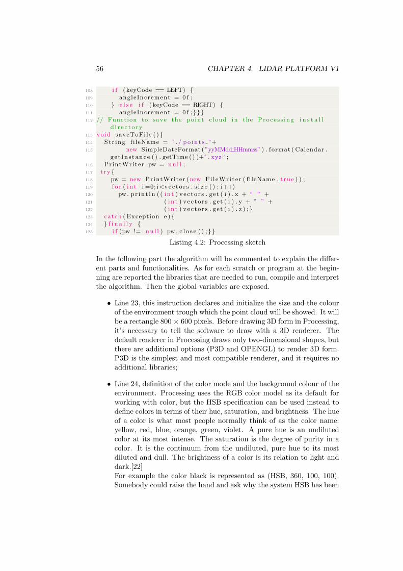
56 CHAPTER 4. LIDAR PLATFORM V1
108 i f ( keyCode == LEFT) 109 angleIncrement = 0 f ;110 e l s e i f ( keyCode == RIGHT) 111 angleIncrement = 0 f ;112 // Function to save the po int c loud in the Proce s s ing i n s t a l l
d i r e c t o r y113 void saveToFi le ( ) 114 St r ing f i leName = ” . / p o i n t s ”+115 new SimpleDateFormat ( ”yyMMdd HHmmss” ) . format ( Calendar .
g e t In s tance ( ) . getTime ( ) )+” . xyz” ;116 PrintWriter pw = n u l l ;117 t ry 118 pw = new PrintWriter (new Fi l eWr i t e r ( f i leName , t rue ) ) ;119 f o r ( i n t i =0; i<ve c t o r s . s i z e ( ) ; i++)120 pw. p r i n t l n ( ( i n t ) v e c t o r s . get ( i ) . x + ” ” +121 ( i n t ) v e c t o r s . get ( i ) . y + ” ” +122 ( i n t ) v e c t o r s . get ( i ) . z ) ;123 catch ( Exception e ) 124 f i n a l l y 125 i f (pw != n u l l ) pw . c l o s e ( ) ;
Listing 4.2: Processing sketch
In the following part the algorithm will be commented to explain the differ-ent parts and functionalities. As for each scratch or program at the begin-ning are reported the libraries that are needed to run, compile and interpretthe algorithm. Then the global variables are exposed.
• Line 23, this instruction declares and initialize the size and the colourof the environment trough which the point cloud will be showed. It willbe a rectangle 800 × 600 pixels. Before drawing 3D form in Processing,it’s necessary to tell the software to draw with a 3D renderer. Thedefault renderer in Processing draws only two-dimensional shapes, butthere are additional options (P3D and OPENGL) to render 3D form.P3D is the simplest and most compatible renderer, and it requires noadditional libraries;
• Line 24, definition of the color mode and the background colour of theenvironment. Processing uses the RGB color model as its default forworking with color, but the HSB specification can be used instead todefine colors in terms of their hue, saturation, and brightness. The hueof a color is what most people normally think of as the color name:yellow, red, blue, orange, green, violet. A pure hue is an undilutedcolor at its most intense. The saturation is the degree of purity in acolor. It is the continuum from the undiluted, pure hue to its mostdiluted and dull. The brightness of a color is its relation to light anddark.[22]For example the color black is represented as (HSB, 360, 100, 100).Somebody could raise the hand and ask why the system HSB has been
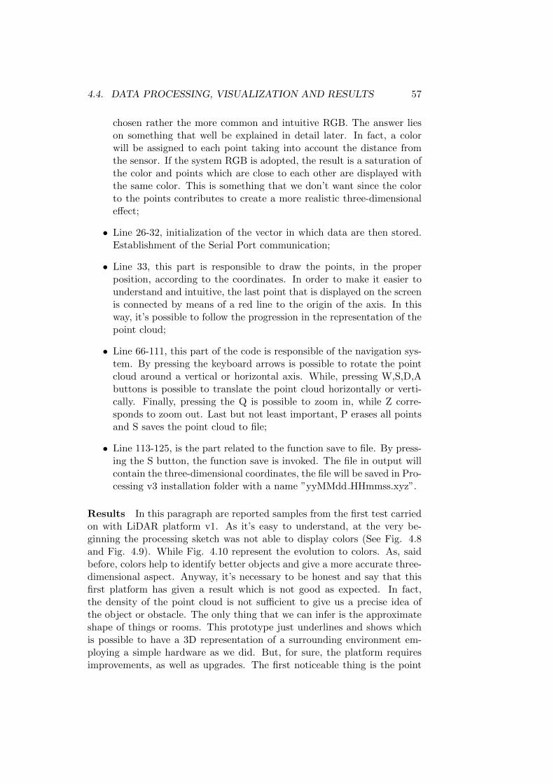
4.4. DATA PROCESSING, VISUALIZATION AND RESULTS 57
chosen rather the more common and intuitive RGB. The answer lieson something that well be explained in detail later. In fact, a colorwill be assigned to each point taking into account the distance fromthe sensor. If the system RGB is adopted, the result is a saturation ofthe color and points which are close to each other are displayed withthe same color. This is something that we don’t want since the colorto the points contributes to create a more realistic three-dimensionaleffect;
• Line 26-32, initialization of the vector in which data are then stored.Establishment of the Serial Port communication;
• Line 33, this part is responsible to draw the points, in the properposition, according to the coordinates. In order to make it easier tounderstand and intuitive, the last point that is displayed on the screenis connected by means of a red line to the origin of the axis. In thisway, it’s possible to follow the progression in the representation of thepoint cloud;
• Line 66-111, this part of the code is responsible of the navigation sys-tem. By pressing the keyboard arrows is possible to rotate the pointcloud around a vertical or horizontal axis. While, pressing W,S,D,Abuttons is possible to translate the point cloud horizontally or verti-cally. Finally, pressing the Q is possible to zoom in, while Z corre-sponds to zoom out. Last but not least important, P erases all pointsand S saves the point cloud to file;
• Line 113-125, is the part related to the function save to file. By press-ing the S button, the function save is invoked. The file in output willcontain the three-dimensional coordinates, the file will be saved in Pro-cessing v3 installation folder with a name ”yyMMdd HHmmss.xyz”.
Results In this paragraph are reported samples from the first test carriedon with LiDAR platform v1. As it’s easy to understand, at the very be-ginning the processing sketch was not able to display colors (See Fig. 4.8and Fig. 4.9). While Fig. 4.10 represent the evolution to colors. As, saidbefore, colors help to identify better objects and give a more accurate three-dimensional aspect. Anyway, it’s necessary to be honest and say that thisfirst platform has given a result which is not good as expected. In fact,the density of the point cloud is not sufficient to give us a precise idea ofthe object or obstacle. The only thing that we can infer is the approximateshape of things or rooms. This prototype just underlines and shows whichis possible to have a 3D representation of a surrounding environment em-ploying a simple hardware as we did. But, for sure, the platform requiresimprovements, as well as upgrades. The first noticeable thing is the point

58 CHAPTER 4. LIDAR PLATFORM V1
Figure 4.8: Scan 1
Figure 4.9: Scan 2
cloud density: it’s not enough to show with precision the scanned objects.For this reason, the next version should improve dramatically this param-eter. In the following section new proposal to solve this problem will bepresented.
4.5 Towards LiDAR v2
The first step, has been to find out the critical parts of our project, start-ing from a free flow of thoughts or brainstorming. But, as well known, isnot possible to randomly presents the list that has emerged, so the secondstep has been to sort that list. From the most critical to the less critical.In this way is possible to establish a priority and fix these problems fol-lowing a well-defined path and process. It’s not possible to think that the

4.5. TOWARDS LIDAR V2 59
Figure 4.10: Scan 3
Rank Priorities
1Code – algorithm (Servo control, Serial DataTransmission, Data Processing)
2 Motors3 Structure
Table 4.2: Table of enhancement
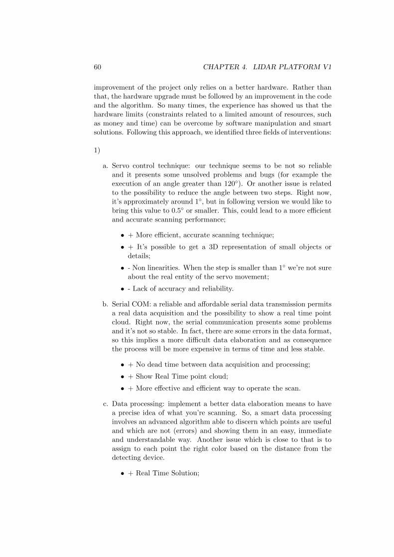
60 CHAPTER 4. LIDAR PLATFORM V1
improvement of the project only relies on a better hardware. Rather thanthat, the hardware upgrade must be followed by an improvement in the codeand the algorithm. So many times, the experience has showed us that thehardware limits (constraints related to a limited amount of resources, suchas money and time) can be overcome by software manipulation and smartsolutions. Following this approach, we identified three fields of interventions:
1)
a. Servo control technique: our technique seems to be not so reliableand it presents some unsolved problems and bugs (for example theexecution of an angle greater than 120). Or another issue is relatedto the possibility to reduce the angle between two steps. Right now,it’s approximately around 1, but in following version we would like tobring this value to 0.5 or smaller. This, could lead to a more efficientand accurate scanning performance;
• + More efficient, accurate scanning technique;
• + It’s possible to get a 3D representation of small objects ordetails;
• - Non linearities. When the step is smaller than 1 we’re not sureabout the real entity of the servo movement;
• - Lack of accuracy and reliability.
b. Serial COM: a reliable and affordable serial data transmission permitsa real data acquisition and the possibility to show a real time pointcloud. Right now, the serial communication presents some problemsand it’s not so stable. In fact, there are some errors in the data format,so this implies a more difficult data elaboration and as consequencethe process will be more expensive in terms of time and less stable.
• + No dead time between data acquisition and processing;
• + Show Real Time point cloud;
• + More effective and efficient way to operate the scan.
c. Data processing: implement a better data elaboration means to havea precise idea of what you’re scanning. So, a smart data processinginvolves an advanced algorithm able to discern which points are usefuland which are not (errors) and showing them in an easy, immediateand understandable way. Another issue which is close to that is toassign to each point the right color based on the distance from thedetecting device.
• + Real Time Solution;
4.5. TOWARDS LIDAR V2 61
• + Easy to display.
All of those three options, software related, are not cost effective, sincethere’s no need to buy anything but just programming and code. Moreover,it’s true that on the internet it’s possible to find some open source softwarethat can guide you in the development of a new application or a new soft-ware part. But at the same time, we should say that we should spend alot of time to make this process smooth and reliable. Anyway, regardingthe motors, it’s necessary to evaluate if a different technology could bringto better performances.
2)
a. To reach a high level of accuracy it’s possible to buy new servos withbetter performances and specs. The main problem that we must faceis the instability of the PWM signal to the servos. In fact, we havetested the servo with an oscilloscope and we have found out that thePWM signal is not stable and oscillates. This can lead to servo rota-tions that are not totally controllable and at the same time uncertain.Considering these problems, it’s a wise decision to take into accountdifferent motor technologies, for example stepper motors. Stepper areused in critical applications where the minimum required step is re-ally small or in task where the precise positioning is an issue. Withan improvement of the motor performances it’s possible to scan moreaccurately the surrounding environment.
• + Accuracy;
• + Reliability;
• + Increase the performance of the whole system;
• - Time and Cost, expensive (especially switch to other technolo-gies);
• - Test in lab;
• - Slow down the scanning speed (↑ accuracy ↓ speed).
3)
a. The mechanical structure is very important because it has to preventthe diffusion of vibrations and place the sensor in a precise position,well fixed and still. The idea is to design a more robust and reliable,stable and safe structure. One thing that we want to avoid is gluedparts (we only accept glued parts if the structure is a demo or trialversion). The final aim will be to design a three-dimensional model ofour structure and manufacture it. The future structure will be madeof metal and we will put a specific attention to make it compact and

62 CHAPTER 4. LIDAR PLATFORM V1
to distribute the mass as close as possible to the axis of rotation of theservos. Moreover, re-designing the structure we will try other solutionsand a different allocation of the motors.
• + Faster scanning process;
• + Robust;
• + Customized (suits perfectly);
• - Requires time and money to re-adjust;
• - high level of complexity related to the manufacturing process.
Chapter 5
LiDAR platform v2
This is, probably, the most important chapter of this work. In fact, it’sfundamental to show that we understood problems and issues emerged inthe first version. And furthermore, we have been able to propose a possiblesolution that suits our requirements and allows to reach the expected qual-ity standard. The decision that has been carried out consists in the radicalchange from servo motors to steppers. This solution brings as consequencethe need to re-write the code that control pan and tilt movements, adaptingit to the new technology that has been implemented. Beside that, the otherparts will substantially remain the same.Just to summarize, the big change is related to hardware. This, involves bigchanges in the software part related to motion control. Other small softwareimplementations will be carried on in this phase, but the impact on the finalproducts is really limited or not substantially relevant. Anyway, consider-ing big changes, it’s mandatory to conceive a new set of experiments, ableto reveal the reliability and the performances of the new motion system inparticular.In the second version of our LiDAR, we adopted stepper motors. On pa-per, this kind of motors can execute very small rotations. If we take forexample, a stepper motor NEMA 171 it can deliver a minimum rotation of1.8 degrees. If a stepper motor is coupled with a micro-stepper driver ispossible to obtain fractions of this angle (typically 1/2, 1/4 , 1/8, 1/32). Sincethe micro-stepper represents an open loop control there’s the need to checkand verify the mechanical accuracy of the motors.
Experimental Structure As consequence of what said before, we arereally interested in the validation of the new pan & tilt movement system.To achieve this, we need to set up a mechanical experiment able to testify theaccuracy of the stepper’s movements. Which are the main characteristics
1NEMA 17 stepper motor is a stepper motor type specified by NEMA. NEMA 17steppers have a 1.7 x 1.7 inch faceplate.
63

64 CHAPTER 5. LIDAR PLATFORM V2
Figure 5.1: Experiment step by step
and features for this experiment?
• able to measure precisely;
• be accurate;
• reliable;
• give a repeatable result.
For the experiment we want to follow a precise and well-organized mind set(See Fig. 5.1). Thanks to that, it will be possible to reduce the failurerate of the experiment to values close to zero. And at the same time, bycontrolling the variables that can affect the result we can get more accurateand reliable results.Starting from the problem and setting the goals of our experiment we canproceed defining the set up. With the word set up we mean the total equip-ment that we need and the whole procedure that we necessarily need tofollow to get a successful experiment. At this stage, it’s at the same timeimportant to take into account external factors which can affect the results,

5.1. STEPPER MOTORS 65
such as temperature, presence of dust, humidity, etc. If one of the things wehave just mentioned (and others) will influence in some ways our activity, wemust consider how and when mitigate their effect. Next step, it’s essentialto check the functionalities of the equipment available, calibrate the instru-ments and correct some biases due to non-zero errors or non-linearities.When this stage has handed, it’s necessary to write a list containing thephases that, step by step, constitute our experiment. Strictly following theprocess guarantees that the measure will be reliable and repeatable. If thenthe result satisfies what was set as the goal of the experiment it’s possibleto say that the process has ended, while if the data elaboration gives un-expected results it’s necessary to reiterate and try a better set up for theexperiment.
5.1 Stepper Motors
Stepper Motors are used in a wide variety of devices ranging from 3D print-ers and CNC machines to DVD drives, heating ducts and even analogueclocks. Stepper motors are DC motors that rotate in precise increments or”steps”. They are very useful when you need to position something veryaccurately. They are used in 3D printers to position the printhead correctlyand in CNC machines where their precision is used to position the cuttinghead.Unlike DC motors, stepper motors are controlled by applying pulses of DCelectricity to their internal coils. Each pulse advances the motor by one stepor by a fraction of a step, the latter is known as ”micro-stepping” and will beexplained shortly. Some people confuse stepper motors with servo motors,but they are actually two different things. A servo motor is unique in thatits motor shaft can be moved to a precise angle, most servos only rotate180 or 270 degrees. A servo motor is ”aware” of its position (as seen in theprevious chapter) and can be moved to a specific angle even if an externalforce moves the motor shaft.Steppers, on the other hand, are ”unaware” of their position. They can bemoved to an exact position in reference to where they start stepping butunlike servos they can be misaligned if their shaft is moved by an externalforce. In many applications a servo is first moved to a ”homing” or refer-ence position before being controlled. Because the move in discrete steps,a stepper motor is not often used where a smooth continuous rotation isrequired, however with the use of gearing and micro-stepping they can ap-proach a smooth rotation and their ability to be very accurately positionedoften outweighs the roughness of their movement.Another advantage stepper motors have over DC motors is the ability tomove at very slow speeds without stalling. They also have a high-torquedensity, so it means that they can provide a high torque if compared to
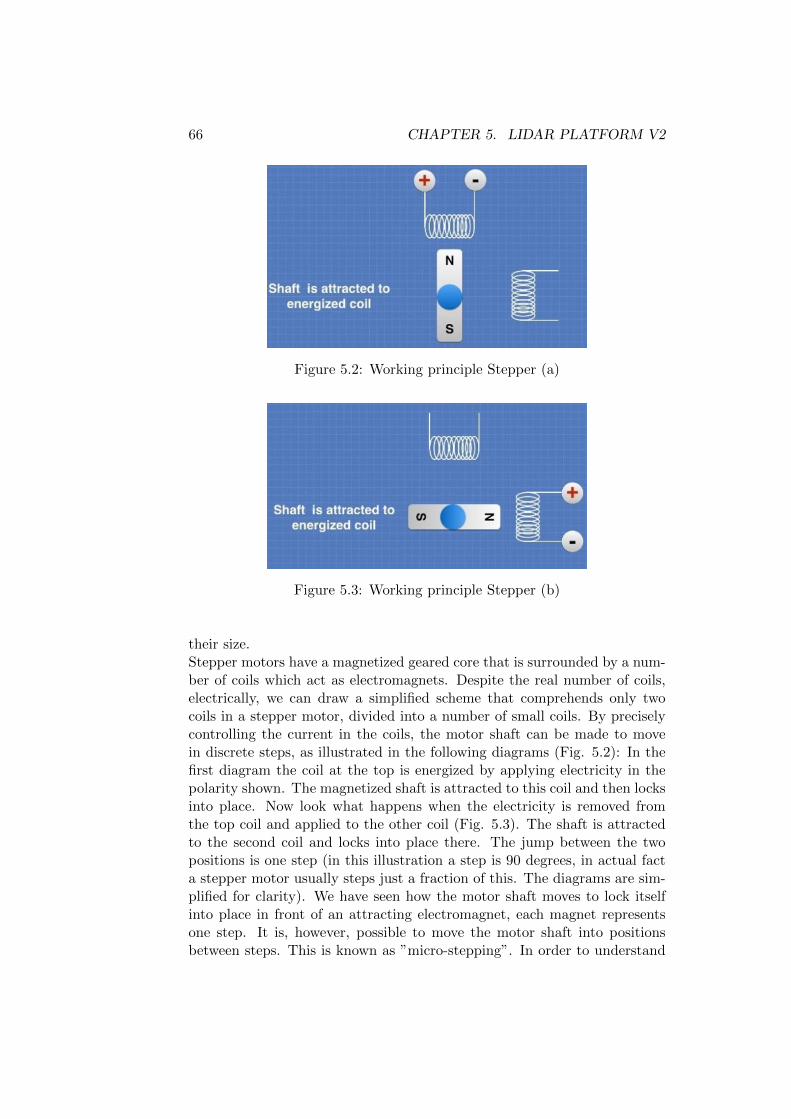
66 CHAPTER 5. LIDAR PLATFORM V2
Figure 5.2: Working principle Stepper (a)
Figure 5.3: Working principle Stepper (b)
their size.Stepper motors have a magnetized geared core that is surrounded by a num-ber of coils which act as electromagnets. Despite the real number of coils,electrically, we can draw a simplified scheme that comprehends only twocoils in a stepper motor, divided into a number of small coils. By preciselycontrolling the current in the coils, the motor shaft can be made to movein discrete steps, as illustrated in the following diagrams (Fig. 5.2): In thefirst diagram the coil at the top is energized by applying electricity in thepolarity shown. The magnetized shaft is attracted to this coil and then locksinto place. Now look what happens when the electricity is removed fromthe top coil and applied to the other coil (Fig. 5.3). The shaft is attractedto the second coil and locks into place there. The jump between the twopositions is one step (in this illustration a step is 90 degrees, in actual facta stepper motor usually steps just a fraction of this. The diagrams are sim-plified for clarity). We have seen how the motor shaft moves to lock itselfinto place in front of an attracting electromagnet, each magnet representsone step. It is, however, possible to move the motor shaft into positionsbetween steps. This is known as ”micro-stepping”. In order to understand

5.1. STEPPER MOTORS 67
Figure 5.4: Working principle Stepper (micro stepping)
Figure 5.5: Bipolar Stepper
how micro-stepping works, it’s possible to See Fig. 5.4: In this illustrationthe current has been applied to both coils in an equal amount. This causesthe motor shaft to lock into place halfway between the two coils. This wouldbe known as a ”half step”. The principle can be extended to include quartersteps, eight steps and even sixteenth steps. This is done by controlling theratio of the current applied to both coils to attract the motor shaft to aposition between the coils but closer to one coil than the other. Commonlythis operation is executed by a micro-stepper driver: choose a good qualitydriver is quite important to reduce vibrations and for smooth operations.By using micro-stepping, it is possible to move the shaft of a stepper motorto a fraction of a degree, allowing for extremely precise positioning.Actually, it’s possible to divide stepper motors in two categories: bipolarand unipolar. Since we don’t want to explain everything in detail I’ll justtalk about bipolar stepper (the one we are interested in and the one onwhich the experiment is based and conceived). Bipolar stepper motors, SeeFig. 5.5, consist of two coils of wire (electrically, actually split into sev-eral physical coils) and generally have four connections, two per coil. Thesimplified diagrams of stepper operation presented in the previous sectionare all bipolar stepper motors. An advantage of bipolar stepper motors isthat they make use of the entire coil winding, so they are more efficient.
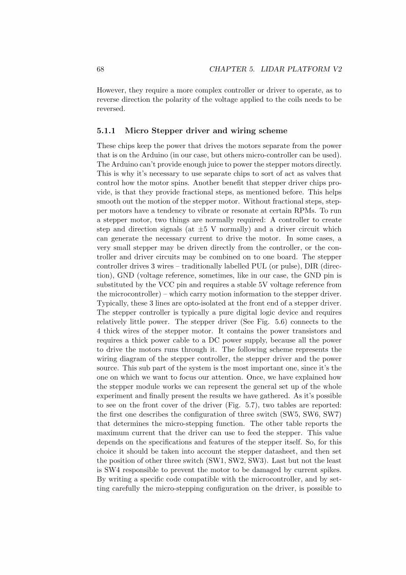
68 CHAPTER 5. LIDAR PLATFORM V2
However, they require a more complex controller or driver to operate, as toreverse direction the polarity of the voltage applied to the coils needs to bereversed.
5.1.1 Micro Stepper driver and wiring scheme
These chips keep the power that drives the motors separate from the powerthat is on the Arduino (in our case, but others micro-controller can be used).The Arduino can’t provide enough juice to power the stepper motors directly.This is why it’s necessary to use separate chips to sort of act as valves thatcontrol how the motor spins. Another benefit that stepper driver chips pro-vide, is that they provide fractional steps, as mentioned before. This helpssmooth out the motion of the stepper motor. Without fractional steps, step-per motors have a tendency to vibrate or resonate at certain RPMs. To runa stepper motor, two things are normally required: A controller to createstep and direction signals (at ±5 V normally) and a driver circuit whichcan generate the necessary current to drive the motor. In some cases, avery small stepper may be driven directly from the controller, or the con-troller and driver circuits may be combined on to one board. The steppercontroller drives 3 wires – traditionally labelled PUL (or pulse), DIR (direc-tion), GND (voltage reference, sometimes, like in our case, the GND pin issubstituted by the VCC pin and requires a stable 5V voltage reference fromthe microcontroller) – which carry motion information to the stepper driver.Typically, these 3 lines are opto-isolated at the front end of a stepper driver.The stepper controller is typically a pure digital logic device and requiresrelatively little power. The stepper driver (See Fig. 5.6) connects to the4 thick wires of the stepper motor. It contains the power transistors andrequires a thick power cable to a DC power supply, because all the powerto drive the motors runs through it. The following scheme represents thewiring diagram of the stepper controller, the stepper driver and the powersource. This sub part of the system is the most important one, since it’s theone on which we want to focus our attention. Once, we have explained howthe stepper module works we can represent the general set up of the wholeexperiment and finally present the results we have gathered. As it’s possibleto see on the front cover of the driver (Fig. 5.7), two tables are reported:the first one describes the configuration of three switch (SW5, SW6, SW7)that determines the micro-stepping function. The other table reports themaximum current that the driver can use to feed the stepper. This valuedepends on the specifications and features of the stepper itself. So, for thischoice it should be taken into account the stepper datasheet, and then setthe position of other three switch (SW1, SW2, SW3). Last but not the leastis SW4 responsible to prevent the motor to be damaged by current spikes.By writing a specific code compatible with the microcontroller, and by set-ting carefully the micro-stepping configuration on the driver, is possible to
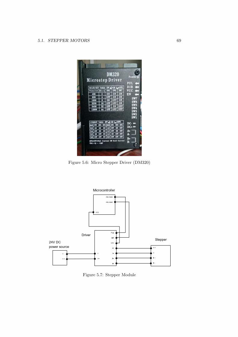
5.1. STEPPER MOTORS 69
Figure 5.6: Micro Stepper Driver (DM320)
Figure 5.7: Stepper Module
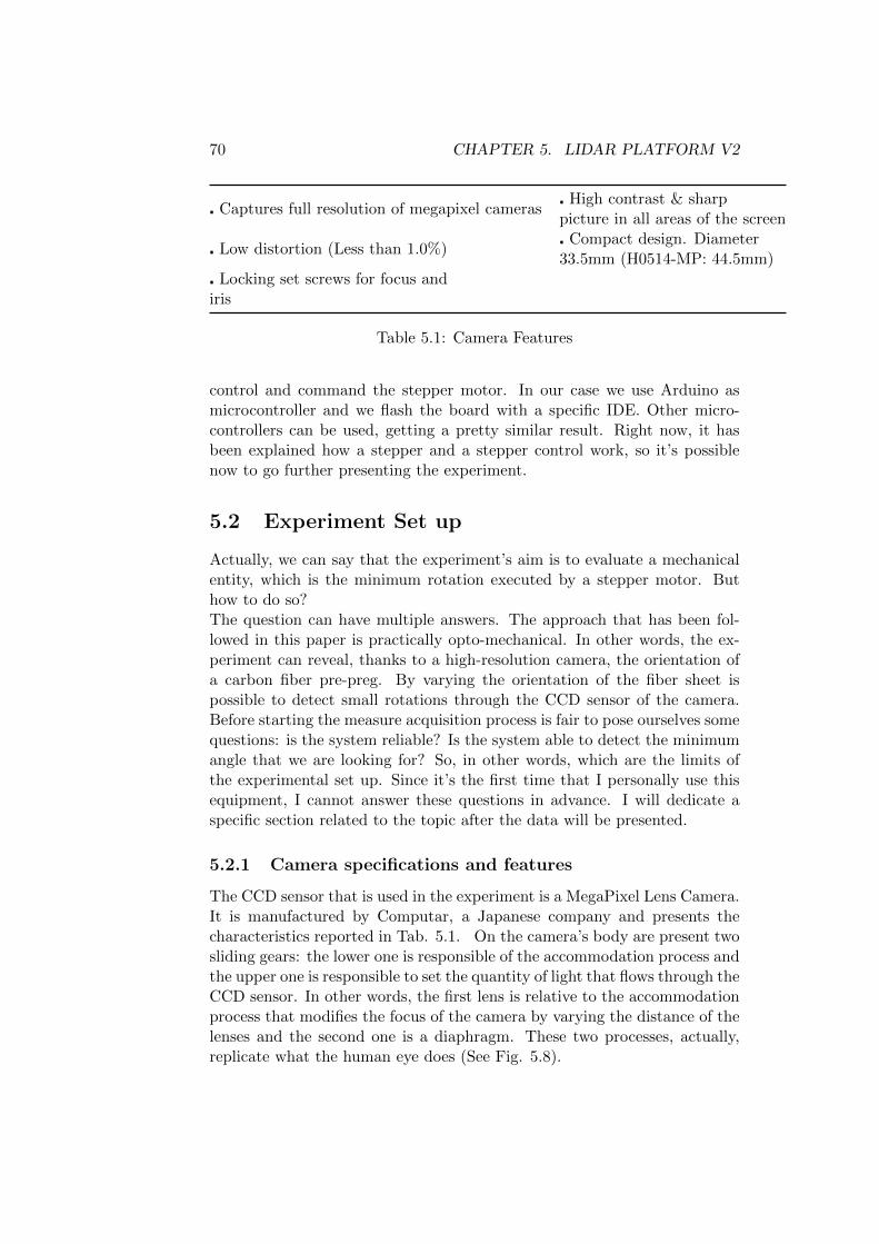
70 CHAPTER 5. LIDAR PLATFORM V2
Captures full resolution of megapixel cameras High contrast & sharppicture in all areas of the screen
Low distortion (Less than 1.0%) Compact design. Diameter33.5mm (H0514-MP: 44.5mm)
Locking set screws for focus andiris
Table 5.1: Camera Features
control and command the stepper motor. In our case we use Arduino asmicrocontroller and we flash the board with a specific IDE. Other micro-controllers can be used, getting a pretty similar result. Right now, it hasbeen explained how a stepper and a stepper control work, so it’s possiblenow to go further presenting the experiment.
5.2 Experiment Set up
Actually, we can say that the experiment’s aim is to evaluate a mechanicalentity, which is the minimum rotation executed by a stepper motor. Buthow to do so?The question can have multiple answers. The approach that has been fol-lowed in this paper is practically opto-mechanical. In other words, the ex-periment can reveal, thanks to a high-resolution camera, the orientation ofa carbon fiber pre-preg. By varying the orientation of the fiber sheet ispossible to detect small rotations through the CCD sensor of the camera.Before starting the measure acquisition process is fair to pose ourselves somequestions: is the system reliable? Is the system able to detect the minimumangle that we are looking for? So, in other words, which are the limits ofthe experimental set up. Since it’s the first time that I personally use thisequipment, I cannot answer these questions in advance. I will dedicate aspecific section related to the topic after the data will be presented.
5.2.1 Camera specifications and features
The CCD sensor that is used in the experiment is a MegaPixel Lens Camera.It is manufactured by Computar, a Japanese company and presents thecharacteristics reported in Tab. 5.1. On the camera’s body are present twosliding gears: the lower one is responsible of the accommodation process andthe upper one is responsible to set the quantity of light that flows through theCCD sensor. In other words, the first lens is relative to the accommodationprocess that modifies the focus of the camera by varying the distance of thelenses and the second one is a diaphragm. These two processes, actually,replicate what the human eye does (See Fig. 5.8).
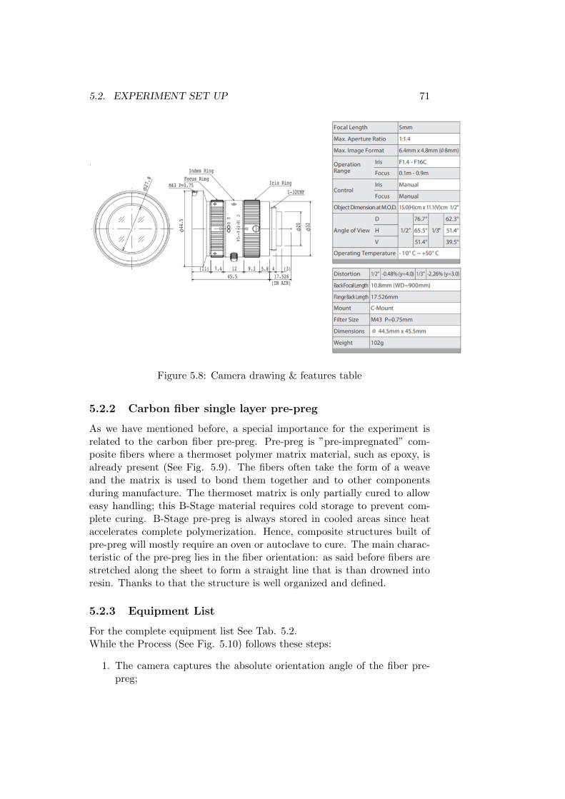
5.2. EXPERIMENT SET UP 71
Figure 5.8: Camera drawing & features table
5.2.2 Carbon fiber single layer pre-preg
As we have mentioned before, a special importance for the experiment isrelated to the carbon fiber pre-preg. Pre-preg is ”pre-impregnated” com-posite fibers where a thermoset polymer matrix material, such as epoxy, isalready present (See Fig. 5.9). The fibers often take the form of a weaveand the matrix is used to bond them together and to other componentsduring manufacture. The thermoset matrix is only partially cured to alloweasy handling; this B-Stage material requires cold storage to prevent com-plete curing. B-Stage pre-preg is always stored in cooled areas since heataccelerates complete polymerization. Hence, composite structures built ofpre-preg will mostly require an oven or autoclave to cure. The main charac-teristic of the pre-preg lies in the fiber orientation: as said before fibers arestretched along the sheet to form a straight line that is than drowned intoresin. Thanks to that the structure is well organized and defined.
5.2.3 Equipment List
For the complete equipment list See Tab. 5.2.While the Process (See Fig. 5.10) follows these steps:
1. The camera captures the absolute orientation angle of the fiber pre-preg;
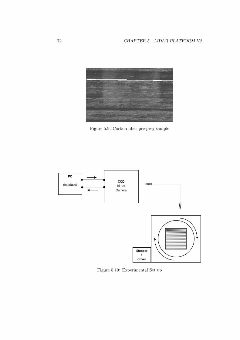
72 CHAPTER 5. LIDAR PLATFORM V2
Figure 5.9: Carbon fiber pre-preg sample
Figure 5.10: Experimental Set up
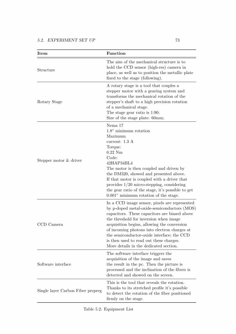
5.2. EXPERIMENT SET UP 73
Item Function
Structure
The aim of the mechanical structure is tohold the CCD sensor (high-res) camera inplace, as well as to position the metallic platefixed to the stage (following).
Rotary Stage
A rotary stage is a tool that couples astepper motor with a gearing system andtransforms the mechanical rotation of thestepper’s shaft to a high precision rotationof a mechanical stage.The stage gear ratio is 1:90;Size of the stage plate: 60mm;
Stepper motor & driver
Nema 171.8 minimum rotationMaximumcurrent: 1.3 ATorque:0.22 NmCode:42HAP34BL4The motor is then coupled and driven bythe DM320, showed and presented above.If that motor is coupled with a driver thatprovides 1/20 micro-stepping, consideringthe gear ratio of the stage, it’s possible to get0.001 minimum rotation of the stage.
CCD Camera
In a CCD image sensor, pixels are representedby p-doped metal-oxide-semiconductors (MOS)capacitors. These capacitors are biased abovethe threshold for inversion when imageacquisition begins, allowing the conversionof incoming photons into electron charges atthe semiconductor-oxide interface; the CCDis then used to read out these charges.More details in the dedicated section.
Software interface
The software interface triggers theacquisition of the image and savesthe result in the pc. Then the picture isprocessed and the inclination of the fibers isdetected and showed on the screen.
Single layer Carbon Fiber prepreg
This is the tool that reveals the rotation.Thanks to its stretched profile it’s possibleto detect the rotation of the fiber positionedfirmly on the stage.
Table 5.2: Equipment List
74 CHAPTER 5. LIDAR PLATFORM V2
2. The stepper motor steps by a certain number of steps (this numberis set up precisely by coding the micro-controller) as previously de-scribed. At the same time, the stage will rotate, and the orientationof the fiber will change. Now, it’s necessary to take into account thefact that one step of the stepper motor corresponds to 1:90 degreesrotation of the platform if the micro-stepping is avoided. Conversely,the angle should be adjusted dividing by the micro-stepping factor.
Examples:
Stepper minimum step 1.8;no micro-stepping /1;Gear ratio: 1/90;⇒ rotary stage rotation per step: 0.02;
Stepper minimum step 1.8;micro-stepping 1/2 ;Gear ratio: 1/90;⇒ rotary stage rotation per step: 0.01;
Stepper minimum step 1.8;micro-stepping 1/4;Gear ratio: 1/90;⇒ rotary stage rotation per step: 0.005.
3. The camera is triggered a second time to capture the new picture ofthe fiber orientation;
4. Thanks to simple calculation is possible to obtain the ∆ rotation (be-tween status 1 and status 2). See Fig. 5.11 to have an intuitive andvisual idea of the whole process.
By knowing the number of steps that the stepper has executed and takinginto account what has been said in point 2), it’s possible to make a compar-ison between the expected value and the value that has been measured bythe camera with the second picture. One thing is valuable to be underlined:if we analyze the process we understand that the measure does not dependon the absolute values gathered by the camera. In fact, we are interestedin the difference between the two values rather than the absolute numbers.This means that we can tolerate some errors related to non-zero alignment,since the error will, presumably, affect the two measures in the same way.This is a very good result, in fact we have as consequence a stable and re-liable method to measure what we are looking for. The only thing that isunknown at this point is if the camera will be able to detect a single stepof the whole system. In that case, it won’t be a problem let the motor step
5.3. EXPERIMENTAL DATA 75
by a precise number of steps (i.e. 10, 100, 1000, 10000, etc.) and thencheck the amplitude of the average step, by simply dividing the angle thatis measured with the camera by the number of steps. Last but not the leastwe need to make some annotations. Talking about the experimental set up,it’s necessary to say that:
• The fiber should be well positioned and fixed on the rotary platform,that lies on the rotary stage. In detail, four pieces of thin tape hasbeen attached on the plate and the Pre-Preg sheet has been firmlyanchored;
• The Pre-preg sheet has been cleaned with some alcohol in order toremove some pollution and dirt from the surface. This step requirespatience since it’s very easy to damage the carbon fiber layer. So,if the sheet is damaged the software struggles to recognize the fiberpattern and at the same time the output measure is not accurate;
• A special light has been used to illuminate the fiber sample, in thisway it’s possible to increase the contrast factor and this helps a lot inthe patter recognition of the fiber;
• As we have mentioned before the camera presents two sliding gears.It’s important to calibrate the focus and the diaphragm aperture toincrease the resolution and contrast of the picture.
5.3 Experimental Data
In addition of what reported before, we can spend some more words on themethodology that will be used during the data gathering process. First ofall, a micro-stepping factor will be set, and for each fms, 4 or 5 measurementswill be taken, especially the ones related to 10-100-1000-10000 steps. In thatway, we want to test if the stepper is accurate, but moreover we want tounderline which are the boundaries and the limit of our set up. Only then, itwill be possible to make a diagram that expresses ∆
nsversus ns itself. Just to
be clear and complete, the process already presented in the previous chapterwill be explained with pictures (only one measurement) and then the otherdata will be reported in charts.
5.3.1 Data Report
The first set of measurements is obtained by using a micro-stepping factorequal to 1/2 . As shown in the following pictures, the camera has beentriggered twice: the first time, as reference, while the second time, after therotation, to measure the new angular position of the fiber. In this case the

76 CHAPTER 5. LIDAR PLATFORM V2
Figure 5.11: Computational Process
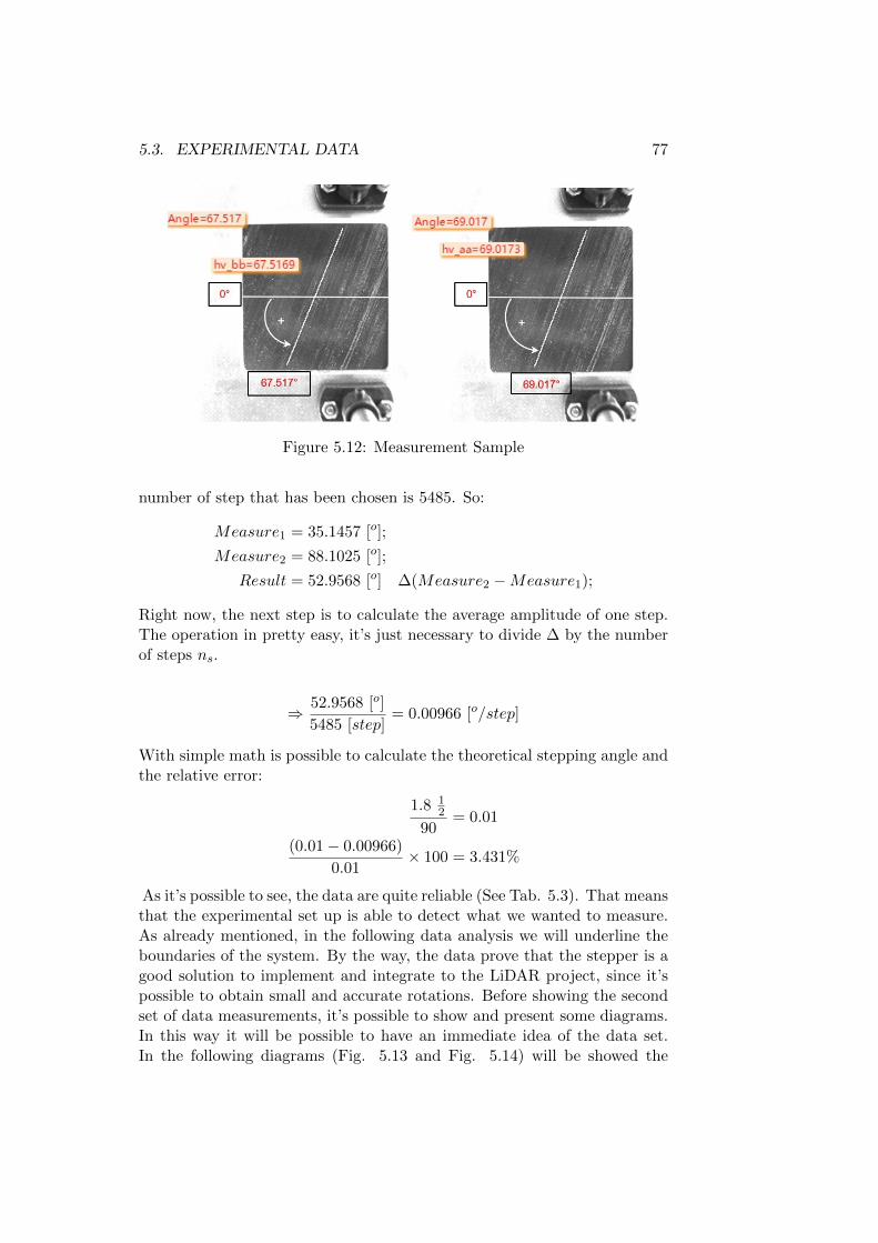
5.3. EXPERIMENTAL DATA 77
Figure 5.12: Measurement Sample
number of step that has been chosen is 5485. So:
Measure1 = 35.1457 [o];
Measure2 = 88.1025 [o];
Result = 52.9568 [o] ∆(Measure2 −Measure1);
Right now, the next step is to calculate the average amplitude of one step.The operation in pretty easy, it’s just necessary to divide ∆ by the numberof steps ns.
⇒ 52.9568 [o]
5485 [step]= 0.00966 [o/step]
With simple math is possible to calculate the theoretical stepping angle andthe relative error:
1.8 12
90= 0.01
(0.01− 0.00966)
0.01× 100 = 3.431%
As it’s possible to see, the data are quite reliable (See Tab. 5.3). That meansthat the experimental set up is able to detect what we wanted to measure.As already mentioned, in the following data analysis we will underline theboundaries of the system. By the way, the data prove that the stepper is agood solution to implement and integrate to the LiDAR project, since it’spossible to obtain small and accurate rotations. Before showing the secondset of data measurements, it’s possible to show and present some diagrams.In this way it will be possible to have an immediate idea of the data set.In the following diagrams (Fig. 5.13 and Fig. 5.14) will be showed the
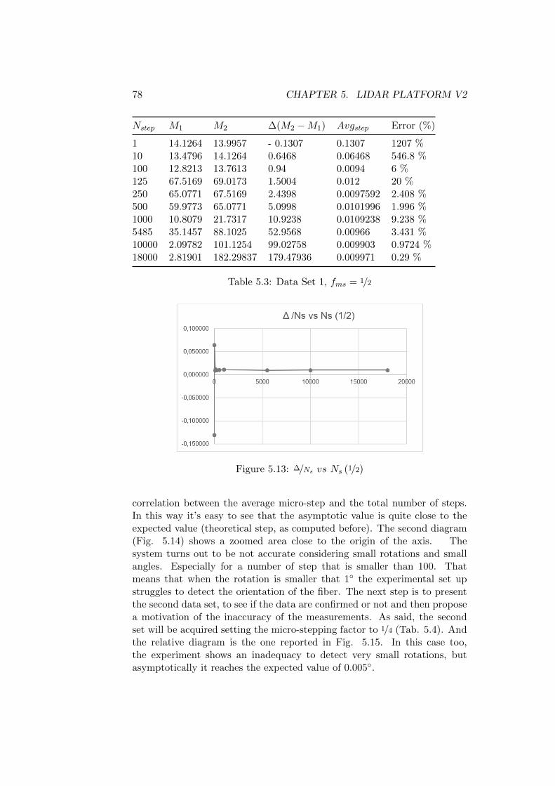
78 CHAPTER 5. LIDAR PLATFORM V2
Nstep M1 M2 ∆(M2 −M1) Avgstep Error (%)
1 14.1264 13.9957 - 0.1307 0.1307 1207 %10 13.4796 14.1264 0.6468 0.06468 546.8 %100 12.8213 13.7613 0.94 0.0094 6 %125 67.5169 69.0173 1.5004 0.012 20 %250 65.0771 67.5169 2.4398 0.0097592 2.408 %500 59.9773 65.0771 5.0998 0.0101996 1.996 %1000 10.8079 21.7317 10.9238 0.0109238 9.238 %5485 35.1457 88.1025 52.9568 0.00966 3.431 %10000 2.09782 101.1254 99.02758 0.009903 0.9724 %18000 2.81901 182.29837 179.47936 0.009971 0.29 %
Table 5.3: Data Set 1, fms = 1/2
Figure 5.13: ∆/Ns vs Ns (1/2)
correlation between the average micro-step and the total number of steps.In this way it’s easy to see that the asymptotic value is quite close to theexpected value (theoretical step, as computed before). The second diagram(Fig. 5.14) shows a zoomed area close to the origin of the axis. Thesystem turns out to be not accurate considering small rotations and smallangles. Especially for a number of step that is smaller than 100. Thatmeans that when the rotation is smaller that 1 the experimental set upstruggles to detect the orientation of the fiber. The next step is to presentthe second data set, to see if the data are confirmed or not and then proposea motivation of the inaccuracy of the measurements. As said, the secondset will be acquired setting the micro-stepping factor to 1/4 (Tab. 5.4). Andthe relative diagram is the one reported in Fig. 5.15. In this case too,the experiment shows an inadequacy to detect very small rotations, butasymptotically it reaches the expected value of 0.005.
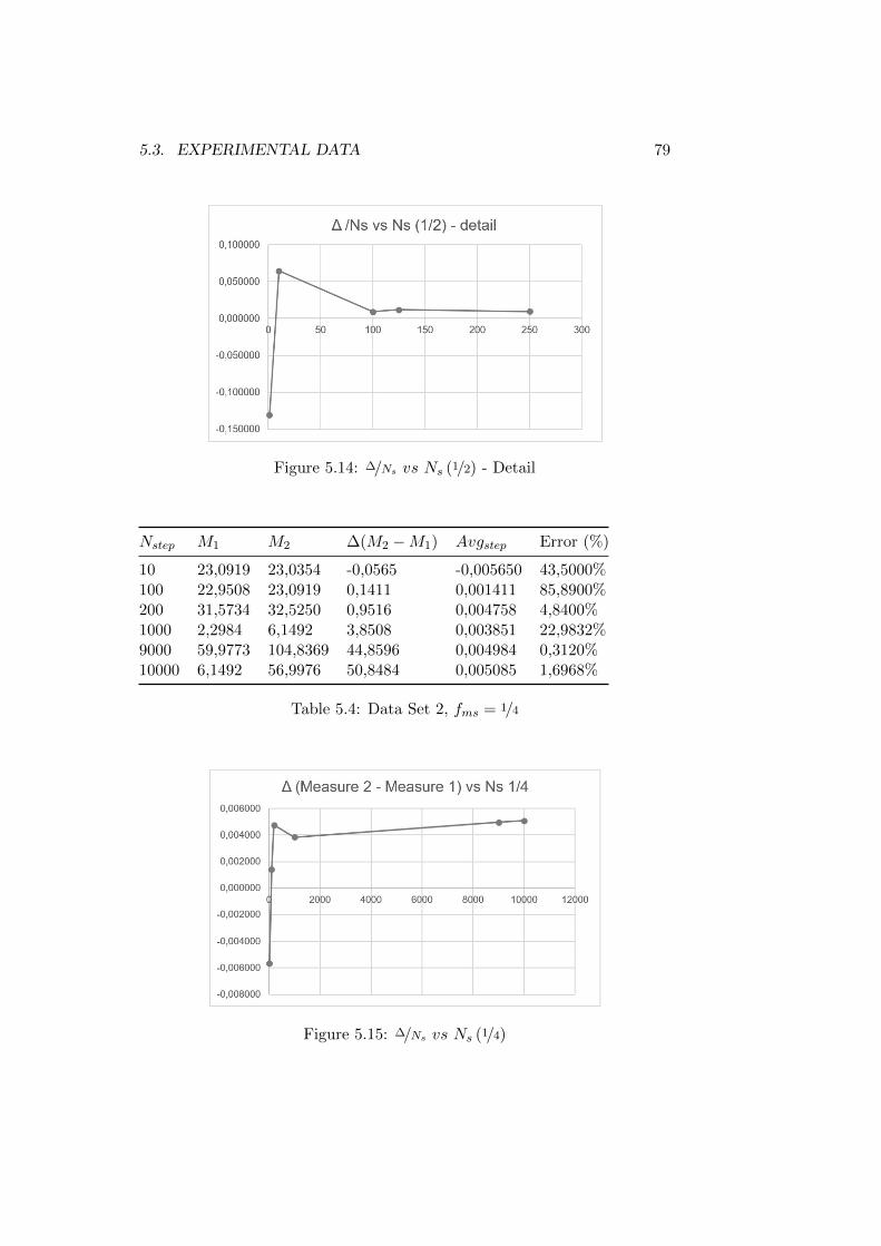
5.3. EXPERIMENTAL DATA 79
Figure 5.14: ∆/Ns vs Ns (1/2) - Detail
Nstep M1 M2 ∆(M2 −M1) Avgstep Error (%)
10 23,0919 23,0354 -0,0565 -0,005650 43,5000%100 22,9508 23,0919 0,1411 0,001411 85,8900%200 31,5734 32,5250 0,9516 0,004758 4,8400%1000 2,2984 6,1492 3,8508 0,003851 22,9832%9000 59,9773 104,8369 44,8596 0,004984 0,3120%10000 6,1492 56,9976 50,8484 0,005085 1,6968%
Table 5.4: Data Set 2, fms = 1/4
Figure 5.15: ∆/Ns vs Ns (1/4)
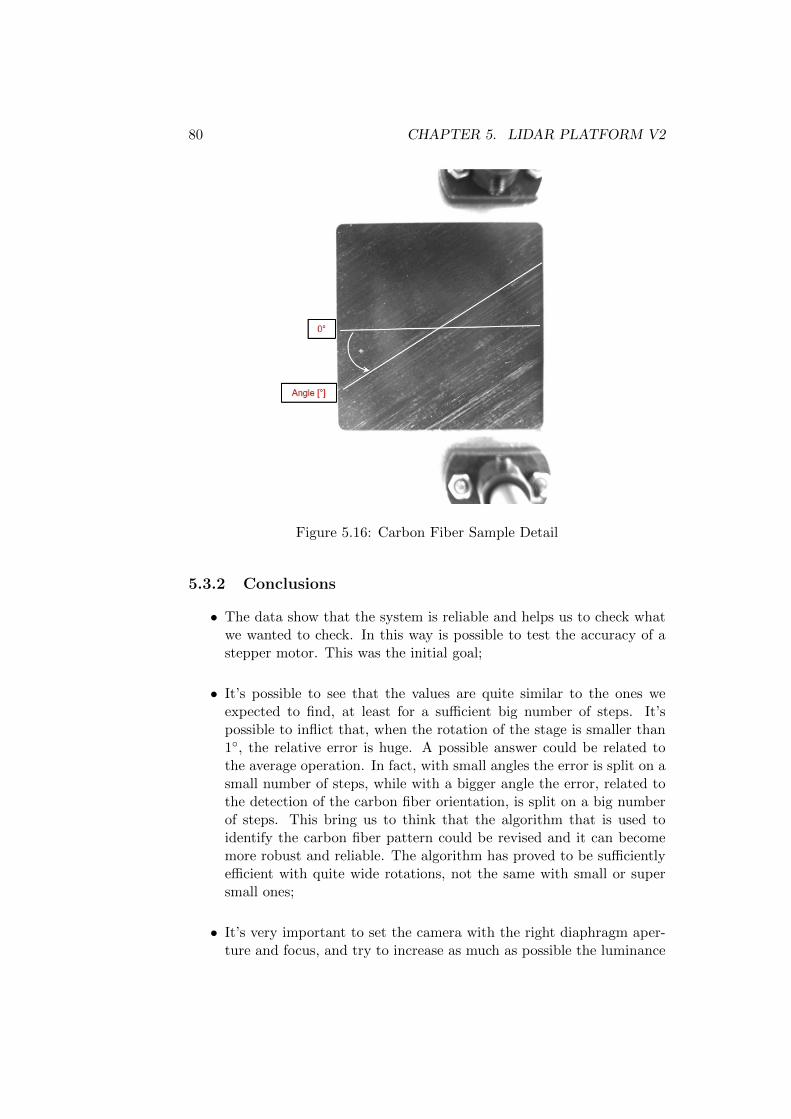
80 CHAPTER 5. LIDAR PLATFORM V2
Figure 5.16: Carbon Fiber Sample Detail
5.3.2 Conclusions
• The data show that the system is reliable and helps us to check whatwe wanted to check. In this way is possible to test the accuracy of astepper motor. This was the initial goal;
• It’s possible to see that the values are quite similar to the ones weexpected to find, at least for a sufficient big number of steps. It’spossible to inflict that, when the rotation of the stage is smaller than1, the relative error is huge. A possible answer could be related tothe average operation. In fact, with small angles the error is split on asmall number of steps, while with a bigger angle the error, related tothe detection of the carbon fiber orientation, is split on a big numberof steps. This bring us to think that the algorithm that is used toidentify the carbon fiber pattern could be revised and it can becomemore robust and reliable. The algorithm has proved to be sufficientlyefficient with quite wide rotations, not the same with small or supersmall ones;
• It’s very important to set the camera with the right diaphragm aper-ture and focus, and try to increase as much as possible the luminance

5.4. NEW STRUCTURE 81
contrast:
Cw =(Ls − Lb)
LbWhere Cw indicates the luminance contrast, Ls the luminance of thetarget object and Lb the luminance of the background;
• It’s important too to pay attention to the positioning of the carbonfiber on the metallic plate. Some vibrations, or accidental collision(with other structural parts) can modify its position and give wrongresults;
• At the same time is relevant the quality of the carbon fiber that isused. Generally, when the carbon fiber is flexible and malleable it’smore difficult to recognize the pattern. That’s why is recommended topartially activate the resin through heat, UV light or other equivalentmethods;
• The adoption of the stepper technology has proved to be the rightsolution to improve the density of the LiDAR point cloud. By couplingad-hoc electrical driving systems and mechanical system is possibleto obtain densities close to 1Million points, and at the same timeguarantee a high level of accuracy.
5.4 New Structure
Another terrific improvement on LiDAR platform v2 is related to the struc-ture. Actually, there’s no much to say: the new structure is solid and morefirm. It allows a better positioning of the sensor as well a better generalstructure stability. The structure has been firstly drawn in SolidWorsTMandthen manufactured in Steel. In order to improve the overall system perfor-mances and reduce the minimum stepper angle we used a mechanical so-lution. On the pan stepper’s shaft is mounted a gear system. The smallgear is linked to the pan motor, while the big one is linked to a secondaryshaft on which the a small platform is mounted. This platform has beenconceived to be the housing of the tilt motor as well as the sensor’s housing.Reducing the speed allows to reduce contextually the minimum angle thatthe pan stepper delivers. The two gears have a ratio 1:5 and they’re mu-tually connected through a belt, specifically designed. Here we have somepictures: See Fig. 5.17a and Fig. 5.17b.
5.5 Results and Scan
In this section the final version of the LiDAR will be presented, showing therelative pictures (See Fig. 5.18a and Fig. 5.18b). Moreover, the results offurther scan will be showed and then commented.

82 CHAPTER 5. LIDAR PLATFORM V2
(a) Mechanical Assembly (b) Mechanical Assembly Exploded
Figure 5.17: Mechanical Assembly, Detail
(a) LiDAR v2, Detail
(b) LiDAR v2, Detail
Figure 5.18: LiDAR v2

5.5. RESULTS AND SCAN 83
(a) Real Picture
(b) Point Cloud LiDAR v2
Figure 5.19: Table and Boxes Scan, v2
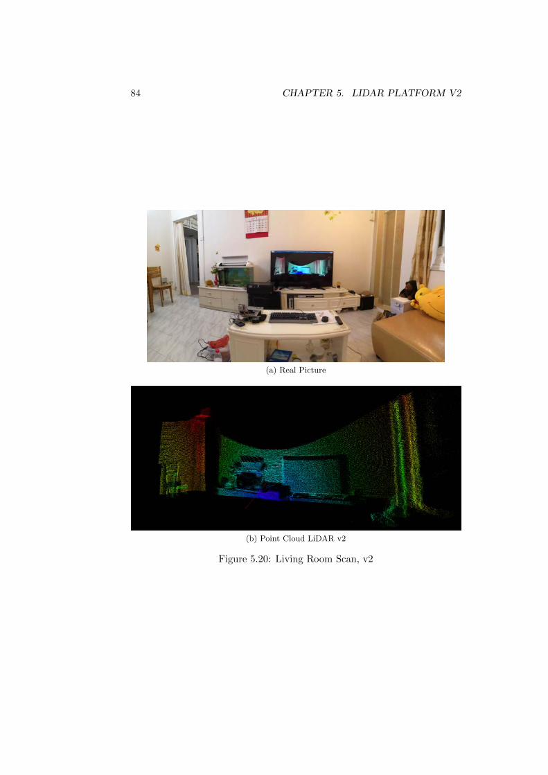
84 CHAPTER 5. LIDAR PLATFORM V2
(a) Real Picture
(b) Point Cloud LiDAR v2
Figure 5.20: Living Room Scan, v2

5.5. RESULTS AND SCAN 85
Figure 5.21: Human Body Scan

86 CHAPTER 5. LIDAR PLATFORM V2
Chapter 6
Conclusions
This last chapter is fundamentally a recap of what has been treated andpresented in this work. The main goal of the project was to develop aversatile LiDAR platform able to scan the surrounding environment with adecent accuracy and quality of the point cloud. We repeat another time thatquality of the point cloud, actually means density: the more dense a pointcloud is, the more accurate the final representation is. Anyway, the maingoal was to meet these requirements, dealing with a constraint on costs. Thefinal platform, indeed, should have cost roughly 250$. With the followinglist the whole process will be recapped and some conclusions or notes willbe added:
1. We started from the basic knowledge, from scratch, studying the singlecomponents and parts of the project, learning the theory and tryingto figuring out how to solve a complex problem as the one we had ininput;
2. Finally, the LiDAR v1 has been designed first and then manufactured:the development of this platform has been challenging and required usto put together a vast knowledge and deploy multidisciplinary skills;basically related to servo motor control, Arduino servo managementand integration, the LiDAR sensor and other various equipment. Butit’s not finished, indeed, the project required us to develop from scratcha brand new visualization environment which allows us to show the realtime point cloud that represents the virtualization of the surroundingreality. This environment has been written on a Java platform calledProcessing v3 (virtual image processing system);
3. Unluckily, LiDAR v1’s performances were not as good as expected. So,after the testing phase, we focused our attention on which were thelimits of the first version and which were the updates or adjustmentsthanks to which LiDAR’s performances could have improved. Only
87
88 CHAPTER 6. CONCLUSIONS
then, the most efficient and profitable solutions has been adopted inversion 2;
4. Then, LiDAR v2 has been released. This second version required animpressive effort, in particular due to the new pan & tilt motor module(brand new technology) and the design of the new platform’ structure.As said, moving from servos to steppers has been a huge leap. So wehad to face lots of unknowns and doubts. In order to understand if thestepper actually suited our application, we conceived a test carried onin the lab, aimed at testing these components, in terms of reliability,accuracy and performance. The test gave us the answers we werelooking for. Beside that, as hinted, a new structure has been released.A final test phase then proved huge improvements in real word scenariorepresentation.
5. Talking about the LiDAR prototype and its possible applications, it’squite easy to say 3D virtual scan and point cloud representation ofinteriors (what we did in the test phase). But then, with furtherimprovements and updates that machine could be used as a low costplatform applicable to:
– Urban planning and modelling (new infrastructures planning incritical existing contexts);
– 3D Building modelling;
– Infrastructure monitoring and control (status check of power lines,railways, ...). This last application is strictly related to my majorand my academic background, so it takes on a truly interestingmeaning.


90 CHAPTER 6. CONCLUSIONS

Bibliography
[1] Robert K. Wysocki, Effective Project Management. Traditional, Agile,Extreme. Fifth edition(2009). ISBN 978-0-470-42367-7.
[2] LIDAR—Light Detection and Ranging—is a remote sensing method usedto examine the surface of the Earth”. NOAA. Archived from the originalon June 4, 2013. Retrieved June 4, 2013.
[3] J. Young, Lidar for Dummies, (2011), Wiley Publishing Inc., ISBN: 978-0-470-94225-3.
[4] Cracknell, Arthur P.; Hayes, Ladson (2007) [1991]. Introduction to Re-mote Sensing (2 ed.). London: Taylor and Francis. ISBN 0-8493-9255-1.OCLC 70765252.
[5] M. Doneus, I. Miholjek, G. Mandlburger, N. Doneus, G. Verhoeven, Ch.Briese, M. Pregesbauer, ”Airborne laser bathymetry for documentationof submerged archaeological sites in shallow water”. ISPRS – Interna-tional Archives of the Photogrammetry, Remote Sensing and SpatialInformation Sciences. Bibcode:2015ISPArXL55...99D.
[6] Chiu, Cheng-Lung; Fei, Li-Yuan; Liu, Jin-King; Wu, Ming-Chee. ”Na-tional Airborne Lidar Mapping and Examples for applications in deepseated landslides in Taiwan”. Geoscience and Remote Sensing Sympo-sium (IGARSS), 2015 IEEE International. ISSN 2153-7003.
[7] G. Vosselman,H. Maas, (2012). Airborne and terrestrial laser scanning.Whittles Publishing. ISBN 978-1-904445-87-6.
[8] S. Lee, J. Joon Im, B. Lee, Leonessa, K. Alexander. ”A real time grid-map generation and object classification for ground based 3D lidar datausing image analysis techniques”. Image Processing (ICIP), 2010 17thIEEE International Conference on image processing. ISSN 1522-4880.
[9] A. Jadhav, D. Gambhir. ”Use of LiDAR in Extraction of 3D City Modelsin Urban Planning”. September 1, 2009. Geospatial World Journal.
91

92 BIBLIOGRAPHY
[10] J. A. Jakubiec, C. F. Reinhart. ”A method for predicting city-wideelectricity gains from photovoltaic panels based on LiDAR and GIS datacombined with hourly Daysim simulations”. 12 May 2013, ELSEVIERSolar Energy 93 (2013) 127–143.
[11] D. Lv, X. Ying, Y. Cui, J. Song, K. Qian, M. Li. ”Research on theTechnology of LIDAR Data Processing”. The 28th Research Institute ofChina Electronics Technology Group Corporation Nanjing, China.
[12] NTSB 2016 Report:”Highway Deaths Lead National Increase in Trans-portation Fatalities”. 11.27.2017. https://www.ntsb.gov/news/press-releases/Pages/PR20171121.aspx
[13] The picture is available here. https://www.continental-automotive.com/Landing-Pages/CAD/Automated-Driving/GlobalHighlights/3D-Flash-Lidar (Continental Website).
[14] Extract from here. https://www.cosworth.com/news/electronic-news/demonstrating-the-car-of-the-future-with-lidar-sensor-technology
[15] Lidar Lite v3 Operation Manual and Technical Specifications. GARMIN
[16] The I2C-Bus Specification Version 2.1. Philips Semiconductors. Jan-uary 2000.
[17] ttps://www.sciencebuddies.org/science-fair-projects/references/introduction-to-servo-motors
[18] https://processing.org/
[19] Ira Greenberg (31 December 2007). Processing: Creative Coding andComputational Art. Apress. pp. 151–. ISBN 978-1-4302-0310-0.
[20] Jeanine Meyer (15 June 2018). Programming 101: The How and Whyof Programming Revealed Using the Processing Programming Language.Apress. pp. 121–. ISBN 978-1-4842-3697-0.
[21] Ira Greenberg (25 March 2010). The Essential Guide to Processing forFlash Developers. Apress. pp. 412–. ISBN 978-1-4302-1980-4.
[22] Casey Reas and Ben Fry. Processing: A Programming Handbook forVisual Designers, Second Edition. December 2014, The MIT Press. 720pages.