AIDA-2020-THESIS-2018-001

AIDA-2020Advanced European Infrastructures for Detectors at Accelerators

Academic Dissertation

Performance Studies of Silicon StripSensors for the Phase-II Upgrade of the

CMS Tracker

Paulitsch, Peter (HEPHY Vienna)

27 April 2018

The AIDA-2020 Advanced European Infrastructures for Detectors at Accelerators projecthas received funding from the European Union’s Horizon 2020 Research and Innovation

programme under Grant Agreement no. 654168.

This work is part of AIDA-2020 Work Package 2: Innovation and outreach.

The electronic version of this AIDA-2020 Publication is available via the AIDA-2020 web site<http://aida2020.web.cern.ch> or on the CERN Document Server at the following URL:

<http://cds.cern.ch/search?p=AIDA-2020-THESIS-2018-001>

Copyright c© CERN for the benefit of the AIDA-2020 Consortium

Unterschrift des Betreuers

HEPHY-LOGO-MANUAL

Thomas Reibnegger | Grafik und Design | 1150 Wien Sechshauserstraße 11/2/3/42 | 0650 / 27 37 137 | die.reibe@gmx.at

2. Logo - HEPHY

Es stehen jeweils verschiedene Grafik Formate des Logos in DEUTSCH und ENGLISCH für Druck und Officeanwendungen zur Verfügung.

2.1 Grafik Formate DEUTSCH und ENGLISCH Vektorformat, Illustrator eps: > CMYK (4C) Modus > Druck > RGB (3C) Modus > für Officeanwendungen > 1-FÄRBIG > Grauwerte > Druck > HEPHY-Logo > Schwarz > Druck > HEPHY-Logo > HALBNEGATIV (weiss und rot) * > Druck

Diese Versionen sind beliebig skalierbar!

Pixelformat, 300 und 72 dpi:

> RGB (3C) Modus für Officeanwendungen > JPG > CMYK (4C) Modus für Druck und Officeanwendungen > TIFF > 1-FÄRBIG > Grauwerte > TIFF > HEPHY-Logo > Schwarz > TIFF und JPG > HEPHY-Logo > HALBNEGATIV (weiss und rot) > TIFF und JPG *

TIFF > CMYK > 300 dpi, JPG > RGB > 72 dpi, Diese Versionen sind nicht größer skalierbar!

* Das Halb-Negativ sollte nur in Ausnahmefällen verwendet werden!

Das Logo darf nur in Rücksprache mit Herrn Thomas Reibnegger bei jeder elektronischen Bearbeitung verändert werden.

CMYK- und RGB-Modus 1-FÄRBIG > Grauwerte

SCHWARZ HALBNEGATIV > weiss und rotDiplomarbeit

Performance Studies of Silicon StripSensors for the Phase-II Upgrade

of the CMS Tracker

ausgeführt am Institut für Hochenergiephysikder Österreichischen Akademie der Wissenschaften

unter der Anleitung vonPrivatdoz. Dipl.-Ing. Dr.techn. Christoph SCHWANDA

undUniv.Lektor Dipl.-Ing. Dr.techn. Thomas BERGAUER

durchPeter PAULITSCH, BSc BSc

Pobersacherstraße 214,9710 Feistritz an der Drau

Wien, am 27.4.2018 Unterschrift

KurzfassungUm 2025 wird der LHC (Large Hadron Collider) zum High-Luminosity LHC ausgebaut.Die Luminosität wird um den Faktor 5 bis 10 erhöht, bis auf 1035 cm-2s-1. Daraus ergebensich neue Anforderungen für die Experimente wie dem Compact Muon Solenoid (CMS),wo auch aufgrund von Alterungserscheinungen (Strahlenschäden) die derzeit eingebautenSi-Sensoren des Spurdetektors („Tracker“) in Zukunft nicht weiter eingesetzt werden kön-nen. Darum, und um die neuen Herausforderungen wie stärkere Strahlungsdosen (durchdie Erhöhung der Kollisionsrate) und höhere Datenraten zu bewerkstelligen, muss derCMS Tracker neu gebaut werden. Prototypen von dazu notwendigen Siliziumstreifend-etektoren werden von den Firmen Infineon und Hamamatsu hergestellt. Diese müssenvon Instituten wie dem Institut für Hochenergiephysik (HEPHY) für den Einsatz quali-fiziert werden.Im Zuge dieser Diplomarbeit führte ich Messungen an diesen Sensor-Prototypen mit Pro-tonen (64 bis 252MeV) am MedAustron und mit Elektronen (5.6GeV) am DeutschenElektronen-Synchrotron (DESY) in Form von Testbeams durch, analysierte die Datenund führte Performance- und Qualitätstests durch. Diese umfassten IV-Charakteristika,Rauschanteil, Cluster-Analysen, Beamprofil-Messungen, Effizienz- und Energiemessun-gen. In Vorbereitung auf die Testbeams testete ich neue Trigger-Szintillatoren bezüglichDunkelrate und Effizienz, des Weiteren das Streifensensor-System mittels einer radioak-tiven Quelle und einem Laser-Testaufbau am HEPHY.Beim ersten Testbeam am MedAustron überstiegen hohe Teilchenraten (bis 1010/s) diemaximal mögliche Prozessierungsrate des Sensorsystems. Des Weiteren dominiertenOccupancy und Pile-Up-Effekte das Signal und verfälschten die gemessene Energiede-position. Während des Testbeams wurde beobachtet, dass die Spannungsversorgungdes Streifensensors in Compliance ging, was zu Spannungseinbrüchen führte. NachÄnderungen im Beschleunigersystem durch das MedAustron-Personal waren niedrigereTeilchenraten (105/s) für den zweiten Testbeam verfügbar. Diese Maßnahmen, ergänztdurch Optimierungen im Aufbau, führten zu einer stabilen Spannungsversorgung und dieAuswertung der Daten zu einer exzellenten Übereinstimmung des ermittelten Bremsver-mögens mit Referenzdaten.Zukünftige Testbeams erfordern umfangreiche Vorbereitungen in Bezug auf Funktion-stests, Standardisierung und Simulation um frühzeitig Designschwächen zu identifizieren.Um in Zukunft bessere Energieauflösungen zu erzielen, ist seitens MedAustron eine scharfdefinierte Teilchenratenkontrolle essentiell, ebenso wie Monitoring des Sensorstromver-brauches in hoher Zeitauflösung. Falls ein Bedarf an Niedrigenergie-Testbeams besteht,ist es essentiell das nichtlineare Verhalten des ALiBaVa-Systems zu analysieren, undeventuell darauf aufbauend den Algorithmus der Analysesoftware zu erweitern. WeitereMaßnahmen sollten den erweiterten Schutz gegen elektromagnetische Störungen um-fassen. Möglicherweise kann auch ein passendes Modell gefunden werden um das elek-tronische Rauschen zu beschreiben und um letztendlich das SNR zu erhöhen.

AbstractIn 2025, the LHC (Large Hadron Collider) will be upgraded to the High-LuminosityLHC. The luminosity will be enhanced by a factor of 5 to 10, up to 1035 cm-2s-1. Thisleads to new challenges for experiments such as the Compact Muon Solenoid (CMS),which is already afflicted by aging effects (radiation damages). Therefore the currentlyinstalled silicon sensors of the track detector ("Tracker") have to be replaced, further-more to carry out higher radiation doses (through raised collision rates) and increaseddata rates. The prototypes of the new sensors are provided by the vendors Infineon andHamamatsu. These have to be qualified for application by institutes like the Instituteof High Energy Physics (HEPHY).For this diploma thesis, I did testbeam measurements on these sensors using protons (64to 252MeV) at MedAustron and electrons (5.6GeV) at Deutsches Elektronen-Synchrotron(DESY), analyzed the data and utilized performance and quality evaluation. Thesemethods include IV characteristics, noise contribution, cluster analysis, beam profilemeasurement, efficiency and energy measurements. In preparation for the testbeams,I tested new trigger scintillators to determine dark rates and efficiency and the stripsensor system using a radioactive source and a laser test stand at the HEPHY.At the MedAustron’s first testbeam, high particle rates (up to 1010/s) exceeded the sen-sor system’s processing rate. Occupancy and pile-up effects dominated the signal anddistorted measured energy depositions. During the testbeam, the bias voltage supplyof the strip sensor showed compliance, leading to voltage drops. After changes madeto the accelerator by MedAustron staff, lower particle rates (105/s) were available atthe second testbeam. These actions, complemented by optimizations in the setup, leadto stable power supply and analysis showed excellent conformity of measured stoppingpower to reference data.Prospective testbeams require extensive preparations in terms of functionality tests,standardization and simulation in advance to identify design flaws. For achieving betterenergy resolution in future, well-defined particle rate control by MedAustron is essen-tial, as well as high time-resolved monitoring the current consumption of the sensor. Ifthere is a demand for low-energy testbeams, it is essential to analyze the non-linear gainbehavior in the upper energy deposition range of the ALiBaVa system. Based on that,one may eventually extend the analysis software algorithm. Further procedures shouldcover protection against electromagnetic interference. Perhaps it will be possible to findan appropriate model to characterize electronic noise contribution to improve SNR.

AcknowledgementsI would first like to thank my head supervisor, Privatdoz. Dipl.-Ing. Dr. ChristophSchwanda of the Austrian Academy of Sciences. He consistently allowed this paper tobe my own work, but steered me in the right direction when I left the path of scientificprecision.Furthermore I would like to thank my other supervisor, Univ.-Lektor Dipl.-Ing. Dr.Thomas Bergauer for his support and introduction to the topic and fundamental physics.His encouragement and immediate help with emerging problems made it possible to mas-ter this thesis efficiently. He provided me a broad spectrum of tasks and assignmentswhich resulted in a good overview of the topic.A very special gratitude goes out to all staff at HEPHY: Johannes Grossmann MSc,Dipl.-Ing. Viktoria Hinger and Dr. Axel König MSc for giving excellent introductions inthe underlying physics and teaching me how to use the required devices and software andfurthermore to Dipl.-Ing. Dominic Blöch, Wolfgang Brandner, Dipl.-Ing. Dr. MarkoDragicevic, Elias Pree MSc, Dipl.-Ing. Stefan Schultschik, Dipl.-Ing. Dr. Manfred Va-lentan and Dipl.-Ing. Hao Yin who assisted me with useful tips, clear explanations andauxiliary work.I would also like to acknowledge the personnel from MedAustron, in particular Univ.Ass.Dipl.-Ing. Dr. Albert Hirtl, Univ.Ass. Dipl.-Ing. Alexander Burker and Felix Ulrich-PurBSc for helping and providing complementary tasks for the work.With a special mention to Daniel Schell MSc and Marius Metzler MSc (both from Karl-sruhe Institute of Technology), I would like to thank the people providing cooperativework at the DESY testbeam.I want to express my gratitude to my close friends Dipl.-Ing. (FH) Roland Rittchen MScMSc, Daniel Steiner MSc and also to my girlfriend Lisa Pirker for proofreading.Last but not least, I would like to thank my family: My sister Dr. Andrea Paulitsch-Buckingham for her proofreading and my parents VR Mag. Dr. Peter Paulitsch andVOL Marina Paulitsch, for providing financial and motivational support to ensure thecompletion of this thesis.This project has received funding from the European Union’s Horizon 2020 Researchand Innovation program under Grant Agreement no. 654168.

Contents

1. Introduction and Background 71.1. Motivation . . . . . . . . . . . . . . . . . . . . . . . . . . . . . . . . . . . 71.2. LHC - Large Hadron Collider . . . . . . . . . . . . . . . . . . . . . . . . . 81.3. CMS experiment . . . . . . . . . . . . . . . . . . . . . . . . . . . . . . . . 10

1.3.1. Subsystems . . . . . . . . . . . . . . . . . . . . . . . . . . . . . . . 111.3.2. Phase-II Upgrade . . . . . . . . . . . . . . . . . . . . . . . . . . . . 14

1.4. MedAustron . . . . . . . . . . . . . . . . . . . . . . . . . . . . . . . . . . . 151.5. DESY - Deutsches Elektronen-Synchrotron . . . . . . . . . . . . . . . . . 16

2. Theory of Particle Detectors 192.1. Interaction of charged particles with matter . . . . . . . . . . . . . . . . . 19

2.1.1. Excitation of electrons: Scintillation . . . . . . . . . . . . . . . . . 192.1.2. Bremsstrahlung . . . . . . . . . . . . . . . . . . . . . . . . . . . . . 192.1.3. Ionizing effects . . . . . . . . . . . . . . . . . . . . . . . . . . . . . 212.1.4. Gaussian distribution . . . . . . . . . . . . . . . . . . . . . . . . . 252.1.5. Landau distribution . . . . . . . . . . . . . . . . . . . . . . . . . . 252.1.6. Vavilov distribution . . . . . . . . . . . . . . . . . . . . . . . . . . 26

2.2. Scintillation detector systems . . . . . . . . . . . . . . . . . . . . . . . . . 272.2.1. Scintillators . . . . . . . . . . . . . . . . . . . . . . . . . . . . . . . 282.2.2. Photomultiplier tubes . . . . . . . . . . . . . . . . . . . . . . . . . 282.2.3. NIM electronics . . . . . . . . . . . . . . . . . . . . . . . . . . . . . 28

2.3. Semiconductor physics and silicon detectors . . . . . . . . . . . . . . . . . 292.3.1. Drift . . . . . . . . . . . . . . . . . . . . . . . . . . . . . . . . . . . 302.3.2. Diffusion . . . . . . . . . . . . . . . . . . . . . . . . . . . . . . . . 312.3.3. Doping and p-n junction . . . . . . . . . . . . . . . . . . . . . . . . 322.3.4. Signal generation, analog readout and signal processing . . . . . . 332.3.5. Segmentation and silicon strip sensors . . . . . . . . . . . . . . . . 342.3.6. Charge sharing and eta value . . . . . . . . . . . . . . . . . . . . . 34

3. Experimental Setup and Preparatory Tests at HEPHY 363.1. Principles of testbeam setups . . . . . . . . . . . . . . . . . . . . . . . . . 36

3.1.1. Telescope . . . . . . . . . . . . . . . . . . . . . . . . . . . . . . . . 363.1.2. Triggering and data acquisition . . . . . . . . . . . . . . . . . . . . 36

3.2. Experimental setting . . . . . . . . . . . . . . . . . . . . . . . . . . . . . . 373.2.1. Scintillator system . . . . . . . . . . . . . . . . . . . . . . . . . . . 373.2.2. Strip sensor readout: The ALiBaVa system . . . . . . . . . . . . . 38

5

3.3. Preparatory scintillator tests . . . . . . . . . . . . . . . . . . . . . . . . . 403.3.1. Dark rate determination . . . . . . . . . . . . . . . . . . . . . . . . 403.3.2. Radioactive source tests with 90Sr . . . . . . . . . . . . . . . . . . 41

3.4. Preparatory strip sensor tests . . . . . . . . . . . . . . . . . . . . . . . . . 433.4.1. IV characteristics . . . . . . . . . . . . . . . . . . . . . . . . . . . . 443.4.2. Radioactive source tests . . . . . . . . . . . . . . . . . . . . . . . . 453.4.3. Laser tests in the clean room . . . . . . . . . . . . . . . . . . . . . 45

3.5. Proton testbeam 1 (TB 1) at MedAustron . . . . . . . . . . . . . . . . . . 473.6. Proton testbeam 2 (TB 2) at MedAustron . . . . . . . . . . . . . . . . . . 483.7. Electron testbeam at DESY . . . . . . . . . . . . . . . . . . . . . . . . . . 50

4. Testbeam Analysis and Results 524.1. Silicon sensor analysis . . . . . . . . . . . . . . . . . . . . . . . . . . . . . 52

4.1.1. Noise and pedestal analysis . . . . . . . . . . . . . . . . . . . . . . 524.1.2. Gain . . . . . . . . . . . . . . . . . . . . . . . . . . . . . . . . . . . 534.1.3. Cluster analysis . . . . . . . . . . . . . . . . . . . . . . . . . . . . . 544.1.4. Beam profiles . . . . . . . . . . . . . . . . . . . . . . . . . . . . . . 554.1.5. Signal histograms . . . . . . . . . . . . . . . . . . . . . . . . . . . . 57

4.2. Energy correction of MedAustron data . . . . . . . . . . . . . . . . . . . . 594.3. Stopping power determination . . . . . . . . . . . . . . . . . . . . . . . . . 614.4. Sensor current at high rate proton beam . . . . . . . . . . . . . . . . . . . 63

5. Conclusions and Suggestions 64

Bibliography 66

Glossary 70

A. Appendix 71A.1. Software used for this thesis . . . . . . . . . . . . . . . . . . . . . . . . . . 71A.2. Important hints for the usage of the ALiBaVa system . . . . . . . . . . . 71A.3. Work input . . . . . . . . . . . . . . . . . . . . . . . . . . . . . . . . . . . 71

6

1. Introduction and Background

1.1. MotivationAs Bertold Brecht insinuates, Galileo Galilei once said "The aim of science is not toopen the door to infinite wisdom, but to set a limit to infinite error."a. Independentfrom its historical validation, this quotation is true in many ways: An important partof science is to limit data error. For example, in particle physics experiments like CMSat the LHC (Chapter 1.2 and 1.3), improved precision of measurements can be achievedby increasing the collision rate to generate more events in reasonable time, in order toimprove statistical significance. The number of collisions per time and bunch overlaparea is defined as luminosity:

L (cm-2s-1) = f n N1 N2A

= f n N1 N24πσxσy

(1.1)

where f is the revolution frequency, n the number of particle bunches in the storage ring,N1 and N2 the number of particles per bunch and A the area of bunch overlap.It is aside from collision energy (which sets an upper limit for the capability of producingnew particles), the most important parameter of a storage ring. Usually the beam profilefollows a Gaussian distribution with σx,y. To determine the number of produced particlesN with a reaction cross section σ over the lifetime T of an experiment, the integratedluminosity Lint is used:

N = σLint = σ

∫ T

0Ldt (1.2)

Since the main goal of colliding beam experiments is to produce particles (in large partat high energies), the detector elements are located in a harsh radiation environment.As one can guess, particle flux increases linear with luminosity, so higher integratedluminosities lead to elevated radiation doses for the surrounding material.A way to increase spatial resolution is downsizing detector elements, to reduce errormargins for tracking and vertexing. However, reducing the detector size leads to newchallenges such as stricter requirements for readout electronics and cooling.By implication, both approaches (increasing spatial resolution and luminosity) are com-mon strategies to improve modern high energy experiments. Not only the detector layouthave to be improved, but also its material properties. Consequently, future acceleratorssuch as the HL-LHC (see Chapter 1.2) and it’s experiments need preparatory researchfor new materials and detector structures.

aBrecht, Life of Galileo (1939)

7

1.2. LHC - Large Hadron ColliderThe Large Hadron Collider is currently (2018) the largest storage ring, featuring thehighest particle energy (6.5 TeV per beam, CERN[1] 2017/07), the largest machine andthe most complex scientific structure to date. It was constructed and is administeredby the European Organization for Nuclear Research (CERN, Organisation européennepour la recherche nucléaire).The achievable collision energy of a proton storage ring is mainly determined by circum-ference r and magnetic field of the dipole magnets B. Now, for the particle’s momentump, one gets:

p = q · r ·B −→ p

[GeVc

]= 0.3 · r[m] ·B[T] (1.3)

At energies in the TeV scale, rest mass of protons (≈1GeV/c2) becomes negligible, henceE ≈ p · c.

circumference 26 659mnominal energy 6.5TeV (protons), 2.76TeV/nucleon (ions)

luminosity 1034 cm-2s-1bunches/beam 2 808 (protons)protons/bunch 1.15·1011bunch spacing 25 ns

average/peak bunch crossing rate 31.6MHz / 40MHzaverage collisions per crossing 20

stored beam energy 360MJcirculating current/beam 540mA

peak dipole field 8.33T

Table 1.1.: Parameters of the Large Hadron Collider (CERN[1], 2018/03)

Furthermore, energy loss by bremsstrahlung (see Chapter 2.1.2) is inverse proportionalto the square of the particle’s mass, so the proton (1836 times the mass of an electron) isfavored for high collision energies in storage rings. However, proton collisionsb producemany unwanted secondary effects, so electrons as elementary particles are still usefulfor experiments, especially in linear accelerators such as the future International LinearCollider (ILC [2]) where bremsstrahlung is not a main limiting factor.

High-Luminosity LHC

For the LHC, an increase in luminosity by a factor of 10, up to 1035 cm-2s-1 is planned tobe accomplished in 2026. Enhanced luminosity means higher particle flux, which leads toincreased radiation doses applied to the detectors, as well as higher data rates. To meetthese new issues, the accelerator infrastructure and the detectors have to be successivelyupgraded. Figure 1.2 illustrates the current (2018) time schedule for the accelerator’s

bprotons are compounds of quarks and gluons

8

Figure 1.1.: Accelerators and interaction points of the Large Hadron Collider(CERN[1], 2018/01)

runs and shutdowns for upgrading the experiments. The planned luminosity as well asthe integrated luminosity is also represented.

Figure 1.2.: Run and shutdown schedule of the LHC for the next decade(CERN[3], 2018/03)

The LHC’s four main experiments (see Figure 1.1)• ALICE - A Large Ion Collider Experiment

• ATLAS - A Toroidal LHC Apparatus

• CMS - Compact Muon Solenoid

• LHCb - LHC-beautyaim at testing the predictions of modern particle physics theories, like the Brout-Englert-Higgs mechanism, furthermore physics beyond Standard Model at energy ranges in theTeV scale, for example search for dark matter, Supersymmetry, (SUSY), extra dimen-sions, but also aspects of heavy ion collisions and precision measurements of knownparticles.

9

1.3. CMS experimentAt LHC, CMS (located at Cessy in France) is the largest experiment in terms of mass.It is designed as a general purpose detector, containing different types of detectors,arranged in interlaced layers, each specialized to a certain particle type (CMS:2008[4],page 1ff).The characteristics of the CMS experiment can be summarized as follows:

• General purpose detector

• Capability of muon identification and measurement of momentum

• For charged particles in general: High momentum resolution and spatial trackresolution in the Inner Tracker

• Good energy resolution for charged elementary and composed particles like mesonsand hadrons

Figure 1.3.: Schematic view of the components of the CMS detector (CERN[1], 2017/07)

10

1.3.1. SubsystemsFigure 1.3 shows a schematic view of the physical CMS structure. Since sensor types inhigh energy physics experiments are sensitive to certain particle properties, CMS has ashell structure of detector components sensitive to different particle types. Figure 1.4illustrates the particle sensitivity of the different detector elements.One of the essential components is the solenoid magnet which gives CMS its name. It

Figure 1.4.: Particle signatures in CMS (Lippmann 2012[5])

consists of a cylindrical superconducting coil and generates a magnetic field of 3.8T at18 kA. The field is confined to the detector volume by a steel return yoke.For determining momentum of charged particles, one way is to track the deflection inthis magnetic field, which is described by the Lorentz force (non-relativistic):

F = q (

E +

v ×B) (1.4)

where q is the charge of the particle,E and

B the electric and magnetic fields and

vthe speed of the particle.When setting

E = 0 (in a tracking system, there is usually no external electric field) and

v ⊥

B (considering the transversal components in the cylinder geometry) this equation

reduces to:F = q v B (1.5)

Identified by the centripetal force F = mv2/r and momentum p = mv, one gets

p = q r B (1.6)

where r is the radius of the circular particle trajectory.Through B is known because it is applied externally, the challenge is to determine ras precise as possible (tracking). It stands to reason that the spatial resolution of thetracker is therefore directly linked to the precision of the momentum measurement.

11

Inner pixel system

The density of produced particles is higher at inner layers, arising from their radial tra-jectories originating at the collision point. For vertexing, this circumstance requires thehighest spatial resolution at the nearest entry point into the detector to achieve highestprecision. Therefore, at this location a pixel sensor with high granularity is used, leadingto high spatial resolution.Both, tracking and vertexing, demand the lowest material budget possible, in otherwords the material deployed has to be minimized. This is caused by the interaction ofparticles with matter which causes deflection through scattering, leading to loss in trackand vertex resolution.The interaction point of CMS is surrounded by a new (installed 2017) Inner Tracker

Figure 1.5.: Inner pixel system since Phase-I Upgrade, compared to the predecessor(Wells 2014[6])

which consists of 1184 silicon pixel sensor modules, arranged in four barrel layers. Phase-IUpgrade (Figure 1.2) of the inner system has already been executed. Figure 1.5 illus-trates the actual layout, compared to its predecessor. The three endcap layers for eachside consist of 672 pixel modules in total. In total, 124 million pixels are installed inthe Inner Tracker (CERN-Phase1-CMS-Pixel[7], page 59ff). Its location nearest to theinteraction point in the beam line leads to the highest radiation doses. Through itshigh granularity, a CO2 cooling system with a capacity of 15 kW is installed to relievethe heat load and allowing temperatures down to -20C without water condensation.(CERN-CMS1-Pixel[7], page 161).

Outer tracking system

Adjacent to the inner pixel tracker, the outer silicon strip tracker consists of 24 244 de-tector modules in four subsystems, each of them encased by a carbon fiber or graphiteframe. The active sensor area of each module varies between 6 243mm2 and 17 202mm2,depending on the module’s location (CMS 2008[4], page 55ff). Each module has 512 or768 strips, read out by 256 channels. The total number of sensor strips is 9.3 million,making up a total active area of 198m2. Compared to the Inner Tracker, the silicon strip

12

sensors have a reduced spatial resolution and less readout channels, therefore a lowergranularity. This may be seen as a disadvantage, however, it leads to lower demandsregarding readout electronics, less complex power supply, and therefore less power dis-sipation. Furthermore, the density of particle tracks decreases with increasing distanceto the collision point, which lowers the need for granularity in Outer Tracker regions.The Outer Tracker geometry is built up of 12 layers in the barrel and 10 layers per endcap. The front-end electronics consists of 128 channel readout chips, whose pipeline is192 elements deep. The sampled signals undergo preamplification and pulse shaping viaan APV25 (Friedl 2011[8]) front-end amplifier, at a frequency of 40 MHz, which matchesthe bunch crossing frequency (see Table 1.1)

Electromagnetic Calorimeter

The purpose of the Electromagnetic Calorimeter (ECAL) is the measurement of particleenergies. It is only able to detect particles interacting via the electromagnetic force.Energy deposition is determined via scintillation (see Chapter 2.2) of lead tungstate(PbWO4) crystals, which are highly dense (8.28 g/cm3) but optically clear. The detec-tor characteristic is linear, what means that produced scintillation light is proportionalto the deposited particle energy. The yield of this material is comparably low (4.5 pho-toelectrons per MeV), which requires efficient photodetectors (CMS 2008[4], page 90).For the barrel, these goals are met by avalanche photodiodes, at a gain of 50 and anactive area of 5·5mm2 for each diode. The quantum efficiency is 75%. A pair of diodesis mounted on each crystal. The crystals are set in a matrix of carbon fibre to keep themoptically isolated.In the endcaps, the lower magnetic field enables the use of vacuum phototriodes. Eachphototriode has an active area of 280mm2, one sensor is mounted on each crystal. Thephototriodes have a quantum efficiency of 22% and a gain of ≈10 (CMS 2008[4], page90ff).

Hadron Calorimeter

For the measurement of high energy hadronic particle jets (induced by the strong in-teraction), the Electromagnetic Calorimeter is surrounded by the Hadron Calorimeter(HCAL). For measuring hadronic energy deposition, it is set up in a sandwich structure(sampling calorimeter), where layers of dense material (brass and steel) alternate to lay-ers of plastic scintillators.The active medium consists of 70.000 tiles of scintillating fibers with wavelength shift-ing; light is guided to hybrid photodiodes (photomultiplier tubes for amplification andavalanche diodes for detection of PMT electrons, gain ≈2000). (CMS 2008[4], page122ff)

Muon system

As the name "Compact Muon Solenoid" suggests, detecting muons is one of the mostimportant tasks of the CMS experiment. As one of the most distinguishable decay

13

channels of the Higgs boson is H → ZZ(∗) → 4l, whereas Z is the Z boson and l areleptons (CMS 2012[9]), muons provide an interesting particle signature. Because muonsare more penetrating than most other particles, the muon system is the outermost layer,installed in the return yoke.The magnetic field (2T) in the muon system is antiparallel to the field of the inner layers(3.8T), leading to a typical S-curve signature of muons. The principle of momentumdetermination is identical to the tracker of the inner layers, by measuring the curvatureof trajectory. For tracking the muons, the system consists of two types of detectors: drifttubes in the central barrel and cathode strip chambers in the end caps. For triggering,resistive plate chambers are installed at both locations.(CMS 2008[4], page 162ff)

1.3.2. Phase-II UpgradeAs mentioned in Chapter 1.2, the detectors of the experiments have to be upgradedto meet the requirements of the HL-LHC. Through elevated collision rates and highertrack densities, the required spatial resolution as well as the resulting data rate increasesover few orders of magnitude (CERN-LHCC: Phase II[10], page 25ff). Higher collisionrates also increase the particle flux, so radiation hardness must be improved to meet theHL-LHC requirements. During the life cycle, HL-LHC is planned to reach an integratedluminosity of 3000 fb-1, 10 times compared to the actual run schedule of 300 fb-1, com-pleted in the end of 2023. At this point, the existing sensors will be afflicted by seriousradiation damage; many of them already failed. Therefore the present detector elementshave to be replaced.As mentioned in Chapter 1.3.1, the Phase-I Upgrade of the inner pixel detector has al-ready been executed. For the Phase-II Upgrade (Figure 1.2), it is planned to install newstrip sensors in the Outer Tracker (Figure 1.6). Prototypes for the upgrade are currentlyprovided by the vendors Infineon and Hamamatsu. Infineonc is an interesting candidatebecause of its geographical proximity to CERN and HEPHY and long-term experiencein semiconductor development and production. P-type sensors are preferred because oftheir superior radiation hardness. To pass the qualification process, multiple parame-ters like electrical characteristics, mechanical stability, optical quality and performanceunder irradiation have to be verified.In this diploma thesis, four different sensor types (three from Infineon, one from Hama-matsu) were investigated related to electrical properties (see Table 3.1). For testing inparticle beam environments, testbeam studies at accelerators (MedAustron in WienerNeustadt and DESY II in Hamburg) were conducted.

clocated in Villach, Austria

14

Figure 1.6.: Sketch of the prospective Outer Tracker layout of Phase-II. TB2S = TrackerBarrel with 2S modules, TBPS = TB with PS modules, TEDD = TrackerEndcap Double-Discs (CERN-CMS2-Tracker[11], page 27)

1.4. MedAustronMedAustron is a proton and heavy iond synchrotron used for proton and heavy iontherapy, medical, biological and high energy physics experiments. Its circumference is78m with 16 dipole and 24 quadrupole magnets. At the testbeams, maximum protonbeam energy was limited to 252.7MeV, but 800MeV should be available through 2018.In order to test the performance of strip sensor prototypes, two testbeams in night shifts(further denoted by "TB 1" and "TB 2") at MedAustron were conducted at irradiationline 1 (see Figure 1.7).

Figure 1.7.: Layout of the MedAustron accelerator (CERN[1], 2017/12)

dC6+ not yet available, should be commissioned during 2018, He2+ maybe in the near future

15

circumference 78menergy range 62.4-800MeV* (p+), 120-400MeV/u (C6+)

beam size (FWHM) 4mmnumber of bunches 1

maximum particles/spill 2 · 1010

maximum intensity 3 · 1010/s (p+), 4 · 108/s (C6+)revolution frequency for p+ 1.3MHz (62.4MeV) to 2.5MHz (252.7MeV)

revolution frequency for ions 470 kHz (7MeV/u)maximum beam current 8mAnominal extraction time 5 s

minimum irradiation time 1msdipole magnets 16

quadrupole magnets 24number of RF cavities 1

Table 1.2.: Beam parameters of the MedAustron synchrotron (Schreiner 2018[12])*800MeV were not available at the testbeams, but should be availablethrough 2018

1.5. DESY - Deutsches Elektronen-SynchrotronDESY is named after its first accelerator (DESY I, first operation in 1964), an electronsynchrotron with a beam energy of 7.4 GeV. At this time, it was the largest device of itstype. 1966, quantum electrodynamics was confirmed by this accelerator. DESY II wastaken into operation in 1987, was used as pre-accelerator for DORIS and PETRA andwas the source for the electron testbeam in this thesis (See Figure 1.9). Later, DESY Iwas upgraded to DESY III (1988), which served as a proton synchrotron (and injectorfor PETRA) until 2007.DORIS (Doppel-Ring-Speicher, "double-ring storage") was DESY’s second circular ac-celerator and its first storage ring with a circumference of 300m. This synchrotronconducted for electron-positron collisions up to 5GeV per beam and was shut down2012 in favor of its successor PETRA III.PETRA (Positron-Elektron-Tandem-Ring-Anlage, "positron-electron tandem-ring facil-ity") was finished in 1978. One of its biggest successes was the discovery of the gluon1979. It is an electron-positron collider with a circumference of 2304 and an energy of19GeV per beam.HERA (Hadron-Elektron-Ring-Anlage, "Hadron-Electron Ring Facility") was DESY’slargest collider, with a circumference of 6336m. It was the world’s first collider usingprimarily superconducting magnets. Electron energies were at 27.5GeV, proton energiesat 920GeV. It was shut down in 2007.

16

Figure 1.8.: Accelerators at DESY

circumference 292.8mejection energy 4.5GeV (DORIS), 6.0GeV (PETRA)bunches/beam 1

electrons/bunch up to 3·1010bunch length (FWHM) 23mm

number of cavities 8max. cavity voltage 13.5MV

cavity radio frequency 499MHzmax E loss per revolution 7.83MeV

E precision (∆E/E) 1.2·10-3

Table 1.3.: Parameters of the DESY II synchrotron (DESY II[13], 2018/02)

Electron beam generation at DESY II testbeam sites

At the testbeam sites at DESY II, the electron beam is not directly extracted, becausethis would have an unacceptable influence to the electrons injected to other experiments(see Chapter 1.5).Instead, a carbon fiber target is placed in the circulating beam of the synchrotron (see

17

Figure 1.9.: DESY II synchrotron with test beam sites and electron/positron extraction(DESY II[13], 2017/12)

Figure 1.9). This produces bremsstrahlung which is converted to electron/positron pairsby a metal plate (converter, Cu or Al). A dipole magnet is used to spread out the forwardelectron/positron beam spectrum. Via a collimator, only a small slice of the incidentbeam is cut out of this spectrum. As deflection of charged particles in a magnetic fielddepends on particle energy and magnetic field (see Equation 1.4), the testbeam user isable to choose electron/positron energy by variation of the dipole magnet coil current(DESY II[13], 2017/12).

18

2. Theory of Particle Detectors

2.1. Interaction of charged particles with matter2.1.1. Excitation of electrons: ScintillationA high energy particle hitting matter can transfer a part of its kinetic energy via inelas-tic collisions. This may lead to electronic excitation and relaxation. Another process isionization, followed by recombination. If these relaxation processes emit photons (usu-ally in the visible or UV spectrum), they are referred to as "scintillation". In an idealscintillator, the radiated light is proportional to the transferred particle energy:

Y (λ) = 〈N(λ)〉E

(2.1)

where Y (λ) is the light yield, N(λ) the number of photons at a specific wavelength andE the deposited energy (Kolanoski 2015[14], page 496).For scintillation, it is important that the emission wavelength is longer than the absorp-tion wavelength (Stokes shift), otherwise the emitted photons would be re-absorbed bythe medium itself. A Stokes shift requires at least two available energy transitions, wherethe relaxation of one intermediate state is non-radiative (vibrational or heat dissipative).

2.1.2. BremsstrahlungWhen charged particles enter matter, they unavoidably interact with the Coulomb fieldsof nuclei (dominant) and other electrons (see Figure 2.1). Assuming no momentum istransferred to a nucleus (fixed target, justified by its high mass) and force is defined bythe change of momentum, the non-relativistic Coulomb force acting on an electron canbe written as:

F = d

p

dt= q Q

4πε0‖r‖3r (2.2)

whereas the point of origin is at the position of the nucleus, q = e is the charge of theelectron, Q = Z e is the charge of the nucleus, r is the distance electron-nucleus and ε0is the vacuum permittivity (electric constant).Since the electron loses energy and momentum, conservation of momentum and energyrequires a photon to be emitted; its energy is given by h · f = E1 − E2. These emittedphotons are the bremsstrahlung. Bremsstrahlung typically has a continuous spectrum(exception: bremsstrahlung created by undulators in free-electron lasers), which becomesmore intense and whose peak intensity shifts toward higher frequencies as the change of

ahttps://en.wikipedia.org/wiki/Bremsstrahlung, 2018/03

19

Figure 2.1.: Bremsstrahlung radiated from an electron in the Coulomb field of a nucleusa

energy of decelerated particles increases.The mean energy loss per path length through bremsstrahlung is approximated by:

−dEdx

∣∣∣∣rad≈ 4αρNA

Z(Z + 1)A

z2(

14πε0

e2

mc2

)2

E · ln(183 · Z−1/3) (2.3)

whereas α ≈ 1/137 is the fine structure constant, ρ is the mass density of the target ma-terial, NA is the Avogadro constant, Z the target’s atomic number, A its mass number,z the charge number of the projectile (1 for electrons), m its mass and E its energy.As Equation 2.3 shows, the radiative contribution is linear to energy, but inverse pro-portional to the square of the projectile’s mass. The proton’s mass is about 1836 timeshigher than the mass of an electron, therefore the radiative losses of electrons are 3.4 mil-lions higher, so it is the dominant energy loss mechanism for particle energies more than100MeV (see Figure 2.2). In contrast to electrons, the energy loss of protons at energiesin the MeV range is dominated by inelastic collisions (see Figure 2.3), so bremsstrahlungis negligible. However, at energies in the GeV scale, the contribution of radiative energyloss becomes dominant.

20

1 0 - 2 1 0 - 1 1 0 0 1 0 1 1 0 2 1 0 3 1 0 41 0 - 3

1 0 - 2

1 0 - 1

1 0 0

1 0 1

1 0 2

1 0 3 c o l l i s i o n r a d i a t i v e t o t a l

stopp

ing po

wer (M

eV cm

² / g)

e n e r g y ( M e V )

Figure 2.2.: Mass stopping power for electrons in silicon as a function of the energy ofthe incident particle (NIST ESTAR[15], 2018/03)

2.1.3. Ionizing effectsBethe-Bloch equation

The Bethe-Bloch formula describes electronic energy loss by the incident of massiveparticlesb. It is derived from inelastic projectile-electron collisions, using the premisethat incident particle energies electron binding energies, so detector electrons can beseen as resting in the lab frame of reference.After few derivation steps, the differential mean energy loss per path length (or stoppingpower) is now given by:

−dEdx

∣∣∣∣coll

= Kz2Z

A

1β2

12 ln 2mec

2β2γ2TmaxI2︸ ︷︷ ︸

semi-relativistic

−β2︸︷︷︸relativistic correction

−δ(βγ)2︸ ︷︷ ︸

density correction

(2.4)

bexcept electrons because they are not distinguishable by means of quantum mechanics

21

where β = v

cand γ = 1√

1− β2 .

symbol name value/unitmec

2 electron mass · c2 0.510998918(44)MeVre classical electron radius e2/4ε0mec

2 2.817940325(28) fmNA Avogadro constant 6.0221415(10)·1023 mol-1K 4πNAre

2mec2 0.307075MeVg-1 cm-2

Tmax maximum transferred kinetic energy eV (nota bene!)z charge of incident particle n · eZ atomic number of absorberA atomic mass of absorber gmol-1I mean excitation energy eV (nota bene!)

δ(βγ) density effect correction

Table 2.1.: Parameters of the Bethe-Bloch equation in high energy physics units(PDG 2007[16])

It should be noted that the stopping power using this formula is highly dependent onthe mass density of the target material. Especially for comparing diverse materials whichcan be in different aggregate states, it is more useful to divide the stopping power by themass density to get the mass stopping power, which now is nearly independent of targetmass density (see Figure 2.3). The Bethe-Bloch formula provides a good description forenergy losses in the momentum range of 0.1 < βγ < 100. At lower momentums thepremise of short interaction time (equivalent to electrons at fixed positions) is not validany more, whereas at higher energies radiative effects increase which are not covered bythe Bethe-Bloch model.The mean range ∆x of a particle can be approximated by integrating the reciprocallinear stopping power 1/S(E) over the continuous energy loss (continuous slowing downapproximation CSDA):

S(E) = dE

dx(2.5)

∆x =∫ ∆x

0dx =

∫ L

0

dE

dEdx =

∫ E0

0

dx

dEdE =

∫ E0

0

1S(E)dE (2.6)

where E0...initial kinetic energy of the incident particle. The fluctuations of ∆x areusually small.In contrast to electrons and photons, hadrons have low stopping power at high energies inthe upper MeV range (≈ 0.7 keV/µm at 100MeV) and high stopping power (≈ 30 keV/µmat 1MeV) in the lower MeV range (see Figure 2.3), where the 1/β2 term of the Bethe-Bloch formula is dominating. In a thick absorber, this leads to the conclusion that energyloss is low close to the entry point and is steadily increasing with penetration depth untilit reaches a maximum immediately before the particles come to rest (recombination andnuclear reactions). This peak is called the "Bragg peak" (see Figure 2.4). The Bragg

22

1 0 - 3 1 0 - 2 1 0 - 1 1 0 0 1 0 1 1 0 2 1 0 3 1 0 4

1 0 0

1 0 1

1 0 2

1 0 3ele

ctron

ic (Me

V cm²

/g)

e n e r g y ( M e V )

e l e c t r o n i c n u c l e a r t o t a l

Figure 2.3.: Mass stopping power for protons in silicon as a function of the energy of theincident particle(NIST PSTAR[15], 2018/02)

peak is only relevant for heavy particles, where absorption and elastic scattering can beneglected. The lower part of the right flank is dominated by absorption of protons bynuclear reactions (Kolanoski 2016[14], page 53ff).Since deposited energy by inelastic scattering is linked to deposited radiation dose

and the depth of the Bragg peak is dependent on particle energy, the potential is givento control the energy deposition depth of hadrons. As one can imagine, this openshuge possibilities in radiation therapy over conventional treatments with photons andelectrons, because applied doses can be focused to the target tissue while sparing thesurrounding healthy organs. Application and research of hadron therapy is the mainoperational purpose of the MedAustron (Chapter 1.4).

23

Figure 2.4.: Relative dose distribution for different particles in water (QD[17], 2018/03)

d-electrons: High energy transfer knock-on

During the passage of massive charged particles through matter, most collisions arecharacterized by comparably small energy transfers T Einc, whereas Einc is thekinetic energy of the incident particle. d-electrons are defined as released electrons havingenough kinetic energy to ionize several other atoms, thus causing a track of secondaryionizations. Figure 2.5 illustrates that most d-electrons are emitted through near-centralcollisions, where the energy transfer is higher.

Figure 2.5.: Energy (left) and angular (right) distribution of d-electron emission for pro-tons as projectiles. This is an approximation for resting shell electrons andhigh energy transfer, so not any more valid at cos θ ≈ 0 (Kolanoski 2016[14])

24

2.1.4. Gaussian distributionFor thick detectors (thickness u particle range), the deposited energy profile follows aGaussian distribution. The probability density function (PDF) is:

p(x) = 1σ√

2πexp

(−(x− µ)2

2σ2

)(2.7)

where σ...standard deviation and µ...mean.For a pure Gaussian distribution, the most probable value (MPV, peak) is equal to themean value. Figure 2.6 shows a Geant4 simulation of the energy deposition of low energyantiprotons in silicon.

Figure 2.6.: Geant4 simulation of the energy deposition of low energy antiprotons insiliconc

2.1.5. Landau distributionFor thin detectors (thickness particle range), the deposited energy profile follows aLandau distribution. The PDF is:

f(λ) = 12πi

∫ c+i∞

c−i∞exp(s ln s+ λs)ds = 1

π

∫ ∞0

exp(−t ln t− λt) sin(πt)dt (2.8)

where s is a scale parameter (s ∈ R+).Figure 2.7 shows a Landau distribution. Its asymmetry is apparent, so the most prob-

able value (λMPV = −0.22278) is different from the mean value. The long tail is causedby high energy secondary electrons (d-electrons, see Chapter 2.1.3), whose energy gainis higher than the average. The main part of these secondary electrons will leave the

chttp://inspirehep.net/record/1265279/, 2018/02

25

Figure 2.7.: Probability density function of a Landau distribution (Kolanoski 2016[14])

detector plane after a few µm, but some will have a trajectory nearly parallel to it,causing many secondary ionizations and therefore a high energy deposition.Like the Gaussian distribution, the Landau distribution has to be transformed for de-scription of energy losses. In real detectors, the measured distribution is always a con-volution of a Landau and at least one Gauss PDF, where the additional Gauss PDFsoriginate from uncertainties of the measurement system.

2.1.6. Vavilov distributionFor discrimination between thick and thin detectors Vavilov (Kolanoski 2016[14], page47) introduced a parameter κ:

κ = ξ

Tmax(2.9)

where ξ is the prefactor of the Bethe-Bloch equation (2.4) times the mean range ∆x(equation 2.6):

ξ = 12K

Z

Aρz2

β2 ∆x (2.10)

Now κ determines which distribution is an adequate approximation:κ ≈ 1 → PDF symmetric, Gauss distribution, thick detector

κ . 0.01 → PDF asymmetric, Landau distribution, thin detectorFor a κ between those values, one has to do a Gauss-Landau convolution or use theVavilov distribution (Kolanoski 2016[14], page 49):

p(λ;κ, β2) = 12πi

∫ c+i∞

c−i∞φ(s)eλsds (2.11)

26

whereas

φ(s) = eCeψ(s), C = κ(1 + β2γE)

ψ(s) = s ln κ+ (s+ β2)(∫ 1

01−exp( −st

κ)

t dt− γE)− κ · exp(−sκ )

γE = 0.5772... (Euler-Mascheroni constant)

2.2. Scintillation detector systemsA scintillation detector system typically consists of four elements:

• Scintillator: The scintillator creates photons by scintillation (see Chapter 2.1.1).

• Lightguide: A lightguide is used for geometrical adaptation from the scintillatorto the photosensor. In many applications, the scintillator is cuboid or prismatic,but the photosensor has a circular entry window.

• Photosensor: For the detection of the photons, different sensor types are used:Photomultiplier tubes (PMTs), avalanche photodiodes (APDs) and silicon photo-multipliers (SiPMs). These types differ in quantum efficiency (10% to 50%), gain(105-9), linearity and rise and dead time (≈10 ps to ns).

• Electronics: The purpose of front-end electronics is preamplification, discrimina-tion and shaping of the current pulse. Typically PMTs have a very high gain, sopreamplification is not necessary for these detector systems.

The signal chain is illustrated in Figure 2.8

Figure 2.8.: Schematic view on a scintillation detector systemd

dhttps://en.wikipedia.org/wiki/Scintillation_counter, 2018/03

27

2.2.1. ScintillatorsFor high energy physics experiments, many different classes of materials are in use: Or-ganic scintillators (solid and liquid), inorganic crystals, glasses, and polymerized plasticscintillators. Each of these scintillator types has typical properties regarding quantumefficiency, yield, linearity, radiation hardness and time constant. An ideal scintillatorshould have following characteristics (Kolanoski 2016[14], page 496):

• High quantum efficiency

• Linearity of yield (see Equation 2.1) in terms of deposited energy

• Transparency of scintillation medium

• Short time constant of the relaxation process for fast signal pulses

• Refraction index of scintillation medium close to the lightguide and/or photosensorfor efficient optocoupling

• Light collection efficiency as high as possible

• Appropriate atomic number Z, for most cases higher is better, but for neutrons alow Z is favored

• For high-radiation applications, of course radiation hardness is crucial

Wavelength shifters are often used to adapt scintillation wavelength to the optimumof photosensors. These are materials which itself absorb and re-emit photons at largerwavelengths.

2.2.2. Photomultiplier tubesA photomultiplier tube (PMT, see Figure 2.8) consists of a photocathode, where in-coming photons knock out photoelectrons (photoelectric effect). These photoelectronsare accelerated and focused towards a dynode system (secondary electron multiplier)via an electric field. When hitting the first dynode, multiple secondary electrons areemitted and on their part accelerated to the next dynode. This process is repeated forall consecutive dynodes until the secondary electrons are collected at an anode. Throughthis multi-stage amplification the overall gain of PMTs is very high (105 to 109) an theresulting signal is directly processible. (Kolanoski 2016[14], page 414ff)

2.2.3. NIM electronicsThe Nuclear Instrumentation Module (NIM) standard defines mechanical and electricalspecifications for electronic modules and their crates used in particle and nuclear physics.The concept of replaceable modules in crates offers advantages in flexibility, interchangeof instruments, reduced design effort, ease in updating and maintaining these instru-ments. The NIM standard also specifies cabling, connectors, impedances and levels for

28

logic signals. NIM signals are defined as negative true (at -16mA into 50 Ω = -0.8V).Typical NIM modules (as used in MedAustron TB 1) are discriminators. Two generalapproaches for discriminators are commonly in use:A leading-edge-discriminator reacts on the rising edge of the signal pulse. It is simpleand easy to use, but different rising times (steepness at different pulse heights) lead touncertainties (time walk) at real-time measurements.By splitting the signal into two identical signals, inverting and damping one, delaying theother and adding them, a constant fraction discriminator is formed (see Figure 2.9). Thecombined signal has a zero-crossing, which can be analyzed via a threshold comparator.The resulting trigger signal is now almost independent from input leading edge steepnessand pulse height. This technique is more complex than a leading-edge-discriminator, butoffers more precision for timestamping or critical real-time applications like time-of-flightmeasurements (Kolanoski 2016[14], page 740ff).

Figure 2.9.: Principle of a constant fraction discriminatore

2.3. Semiconductor physics and silicon detectorsIn semiconductors, there are two types of charge carriers: Electrons (-e) and holes (+e),whereas their concentration in undoped silicon is about 1010 cm-3 for each type. Depend-ing on doping type, the concentrationf differs over many magnitudes of order. The morecommon charge carriers are denoted by "majority carriers" whereas the lesser commonones are referred to as "minority carriers".Quantitative description of charge carrier movement in semiconductors is done by theBoltzmann transport equation, similar to the movement in gases. This is possible due tothe concept of an "effective mass" (meff) of the charge carriers, which expresses bindingforces to the crystal lattice (Kolanoski 2016[14], page 121 and 122).

ehttps://en.wikipedia.org/wiki/Constant_fraction_discriminator, 2018/03ftypically 1010

29

2.3.1. DriftAn external electric field

E causes charge carriers to move along the field direction,

according to the Drude model (without magnetic fields) (Kolanoski 2016[14], page 122ff):

meffv + meff

τ

vdrift = q

E (2.12)

where

• v is the charge carrier velocity

• τ mean time beween collisions (between crystal lattice and valence electrons); timeuntil the next momentum change

• vdrift is the charge carrier drift velocity (charge carrier velocity minus thermalvelocity)

• q = ±e is the electric charge of the carrier

In case of constant drift velocity (v = 0), Equation 2.12 reduces to:

vdrift = qτ

meff

E = µ

E (2.13)

whereas µ is identified to the mobility of charge carriers (electrons and holes have to beconsidered separately).The Drude model is equivalent to the relaxation time approximation of the Boltzmanntransport equation. τ is mainly dependent from temperature, but also from the electricfield strength. Figure 2.10 shows that in case of small fields (E < 103V/cm), it isnearly constant, but in typical fields of semiconductor detectors (E ≈ 106V/cm) thisapproximation is not valid any more. This is caused by higher drift velocity vdrift withincreasing field, but it saturates at fields of E < 105V/cm. (Kolanoski 2016[14], page126)The drift movements of charge carriers lead to a drift current jdrift:

jdrift = q n

vdrift (2.14)

where n is the charge carrier density. This can now be identified with Ohm’s law:jdrift = σ

E = q nµ

E (2.15)

which shows that the electrical conductivity is dependent on charge carrier density andmobility.As mentioned in Chapter 2.3, charge carrier density in a homogeneous material is pre-determined by doping concentration. It should be considered that Equations 2.12 to2.15 stand for both electrons and holes, so they have to be summed up for a completeapproach.

30

Figure 2.10.: Mobility of charge carriers in silicon at 300K (Kolanoski 2016[14])

2.3.2. DiffusionIn homogeneous matter containing charge carriers, spatial charge concentration gradientstend to get compensated through thermal movement and Coulomb forces. According toFick’s first law of diffusion, this leads to a compensating current jdiff until a steady stateis reached:

jdiff = −eD

∇n (2.16)

where D is the diffusion coefficient of the associated charge carrier and n its density.Note that in contrast to Equation 2.14, the current direction is independent of thecharges’ sign, because diffusion currents are always diametrical to concentration gradi-ents.Adding Equations 2.15 and 2.16 results in total currents of charge carriers:

je = −eµene

E − eDe

∇ne

jh = eµhnh

E − eDh

∇nh (2.17)

In an one-dimensional (e.g. through a planar p-n junction) thermal equilibrium thereis no net current, hence for electrons je = 0 (Kolanoski 2016[14], page 127):

µeneEx = −De∂ne∂x

(2.18)

An important connectivity between D and µ is given by the Einstein relation (Kolanoski2016[14], page 128):

Di

µi= kBT

e(2.19)

where kB is the Boltzmann constant and T the Temperature.

31

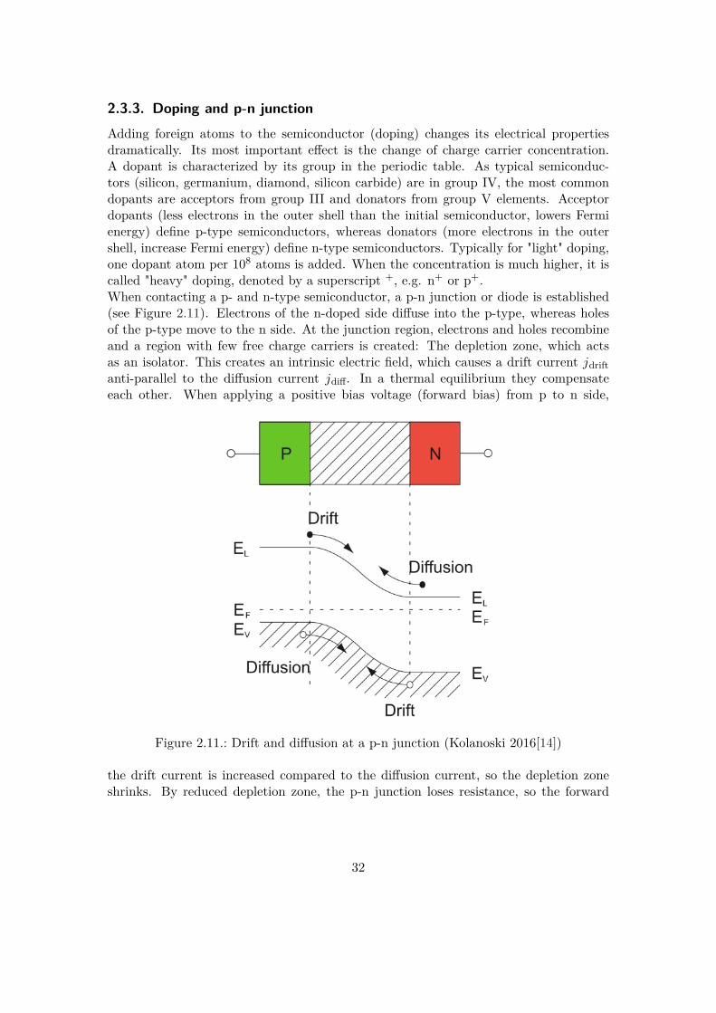
2.3.3. Doping and p-n junctionAdding foreign atoms to the semiconductor (doping) changes its electrical propertiesdramatically. Its most important effect is the change of charge carrier concentration.A dopant is characterized by its group in the periodic table. As typical semiconduc-tors (silicon, germanium, diamond, silicon carbide) are in group IV, the most commondopants are acceptors from group III and donators from group V elements. Acceptordopants (less electrons in the outer shell than the initial semiconductor, lowers Fermienergy) define p-type semiconductors, whereas donators (more electrons in the outershell, increase Fermi energy) define n-type semiconductors. Typically for "light" doping,one dopant atom per 108 atoms is added. When the concentration is much higher, it iscalled "heavy" doping, denoted by a superscript +, e.g. n+ or p+.When contacting a p- and n-type semiconductor, a p-n junction or diode is established(see Figure 2.11). Electrons of the n-doped side diffuse into the p-type, whereas holesof the p-type move to the n side. At the junction region, electrons and holes recombineand a region with few free charge carriers is created: The depletion zone, which actsas an isolator. This creates an intrinsic electric field, which causes a drift current jdriftanti-parallel to the diffusion current jdiff. In a thermal equilibrium they compensateeach other. When applying a positive bias voltage (forward bias) from p to n side,

Figure 2.11.: Drift and diffusion at a p-n junction (Kolanoski 2016[14])

the drift current is increased compared to the diffusion current, so the depletion zoneshrinks. By reduced depletion zone, the p-n junction loses resistance, so the forward

32

current increases. This behavior is described by the Shockley equation:

I(U) = I0

[exp

(eU

kBT

)− 1

](2.20)

whereas e is the elementary charge, U the forward bias voltage and I0 is the reversebias saturation current (the current that flows at reverse bias voltage, but before break-through).By applying a negative bias voltage (reverse bias), the opposite situation is established:The depletion zone grows, which leads to a higher resistance (Kolanoski 2016[14], page285ff). Further increasing the reverse bias may lead to a breakthrough, which can de-stroy the diode if there is a power supply with doesn’t limit current flow.As mentioned in Chapter 2.1.3, ionizing particles create electron-hole pairs, e.g. siliconneeds 3.65 eV. A detector requires a charge-free region, as the charges should only becreated by ionizing particles. In order to optimize the properties of the detector, a re-verse bias high enough to fully deplete the p-n junction is required. This also minimizesthe diode’s capacitance, since a diode can be modeled by a parallel plate capacitor (thedepletion zone acts like a dielectric).

2.3.4. Signal generation, analog readout and signal processingAs mentioned in Chapter 2.1.3, incident high-energy particles transfer momentum todetector electrons which results to an energy loss. This causes electrons to move into theconduction band, equivalent to the creation of electron-hole pairs. These charge carrierscan now move freely through the semiconductor and drift towards the electrodes dueto the applied reverse bias voltage (see Figure 2.13). This induces a current pulse; itsintegral over time gives the charge deposition.The amount of charge carriers received by the electrodes do not cause current generation;the instantaneous change of electrostatic flux lines which end on the electrodes does(Ramo 1939[18]). The Shockley-Ramo theorem states that the instantaneous current jinduced on a given electrode due to the motion of a charge is given by:

j = q · v · Ev (2.21)

whereas q is the electric charge, v the instantaneous velocity and Ev the component ofthe electric field in the direction of v.As seen in Equation 2.21, the electric field generates the drift movement of charge car-riers. Subsequently for high current pulses, high fields (by applying a high reverse biasvoltage) are crucial. High E fields also improve response times through increased mo-bility, as well as improved charge collection efficiency (Spieler 2005[19], page 55).As seen in Figure 2.12, the detector current is transferred outside of the detector byeither AC or DC coupling and amplified by a preamplifier afterwards, which is necessaryfor the next processing stage, the shaper.

33

Figure 2.12.: Detector diode and preamplifier (Grupen 2005[20])

2.3.5. Segmentation and silicon strip sensorsDividing a sensor module in many separate unities and readout channels provides manyadvantages:

• Higher spatial resolution, not only through higher amounts of detector elements,but also through charge sharing effects (only valid for analog readout, see Chap-ter 2.3.6).

• Reduced particle rate per readout channel.

• Distinguishing multiple tracks. Especially useful for jets, common in hadron colli-sions.

• Reduction of area per electrode leads to lower capacitance and electronic noise.

• Improved radiation hardness through smaller leakage currents.

One way for segmentation is to form long but narrow strips of diodes (see Figure 2.13)like for the Outer Tracker of the CMS detector (see Figure 1.6). The detectors used inthis work are strip sensors.

2.3.6. Charge sharing and eta valueIn segmented silicon sensors, maximum achievable spatial resolution is not only givenby segment distance: If a particle hits the area between two segments (most particleswill do that), the generated charge (e-h pairs) will drift to both adjacent segments.Assuming that the lateral segment geometry is symmetrical, the deposited charge shouldbe distance proportional transferred to each segment. Now one can define (using thecenter of gravity method) the η value, for determining the hit position between thetwo segments. In case of 1-dimensional segmentation (strip sensors), η is defined as

34

Figure 2.13.: Schematic view of a strip sensor with charge carrier generation by an inci-dent high energy particle (Hinger 2017[21])

the weighted ratio between the charges collected by the "left" and "right" strip (Hinger2017[21], page 55):

η = QLQL +QR

(2.22)

If the strips are close enough, diffusion (see Chapter 2.3.2) and d-electrons will lead tocharge sharing over multiple strips. This will occur if the dimensions of the generatedcharge cloud are in the same (or larger) scale as the distance between the strips. Byimplication, the center of gravity method for determining the hit position is also workingin this case by summing up over all cluster strips:

y =∑ni=0Qi · yi∑ni=0Qi

(2.23)

where n stands for the size of the cluster, yi is the center position of the strip with indexi, and Qi gives the collected charge for strip i.Spatial resolution using analog readout systems and charge sharing is given by

σ2x = 1

p

∫ p2

− p2x2dx = p2

12 −→ σx = p√12

(2.24)

whereas p is the strip pitch (König 2017[22], page 32).It has to be mentioned that charge sharing is also induced when a particle hits thesensor with a trajectory not perpendicular to the surface, by hitting multiple strips,a bigger cluster is generated. That can be the case in an externally applied magneticfield which bends the particle trajectory. At testbeam environments discussed in thisthesis, the incident particle trajectories are considered to hit the sensor plane almostperpendicularly, because the sensors were not rotated in the beamline.

35

3. Experimental Setup and PreparatoryTests at HEPHY

3.1. Principles of testbeam setups3.1.1. TelescopeMain goal of testbeam setups is to verify the functionality of a device under test (DUT,in most cases a particle detector prototype), electronics, data acquisition (DAQ) or trig-gering systems. Noise is characterized by stochastic fluctuations, but beam trajectoriesare deterministic. To distinguish between desired particles (e.g. coming from the accel-erator) and unrequested particles (e.g. cosmic radiation and background radioactivity,but also particles leaving the setup through scattering), for efficiency tests, geometricalanalysis, tracking and alignment, multiple detector planes are crucial, so a "telescope"is used to reconstruct particle tracks. Figure 3.1 shows a schematic view of a typicaltelescope setup.

Figure 3.1.: Telescope setup with trigger scintillators for testbeams (QD[17], 2017/07)

3.1.2. Triggering and data acquisitionFor triggering, one can distinguish between external triggering (when particle emit timesare known, e.g. in synchronous pulsed sources like the experiments at LHC) and self trig-gering by trigger elements. In a typical testbeam environment a self triggering system isinstalled (see Figure 3.1, usually by scintillators connected to PMTs, see Chapter 3.2.1).In order to reduce undesired triggering, a trigger is usually only fired when a particle hits

36

all triggering scintillators. This can be achieved by using a coincidence circuit, consistingof logical AND gates: A ∧B ∧C. Therefore a trigger is only fired and redirected to theDUT if all detectors A,B and C are firing simultaneously. "Simultaneously" in this caseis given by a timing frame, triggered by the first hit. If all three triggers are fired duringthis time period, the coincidence circuit passes the trigger signal directly to the DUT orto a TLU (trigger logic unit). To reduce false trigger events, the time frame should bemuch smaller than the expected mean time between two incident particles.To reduce noise from unwanted particle trajectories, it is also possible to add a vetoelement, e.g. a scintillator with a hole (where the beam should pass) and subsequentNOT-logic (Kolanoski 2016[14], page 523): A ∧B ∧ C ∧RIn a modern tracking system, hierarchical data acquisition (DAQ) steps are distin-guished:

• When a particle passes all scintillator planes, ideally a trigger signal is fired. Thisis passed to the DUT, which in turn produces an event and the readout systemrecords channel data.

• During the analysis, each event is scanned for correlated clusters (one particle caninduce a signal in more than one channel). Noise contribution is processed by usingpedestals and subtracted from the overall signal.

• After identification of clusters, a hit is generated. A hit contains all informationregarding cluster size, energy deposition, spatial and temporal descriptions.

• By comparing hits and considering telescope geometry (6 coordinates per detectorplane: 3 translations and 3 rotations) the alignment software calculates the relativeposition of the detector planes in a defined coordinate system. Usually it is done viaan optimization algorithm iteratively until convergence and/or a defined numberof iterations.

• When the alignment is finished, a tracking algorithm should be able to reconstructparticle trajectories through the testbeam setup.

3.2. Experimental setting3.2.1. Scintillator systemEach scintillator triggering system consisted of a fast timing anthracene-doped polyvinyl-toluene (PVT) scintillator Eljen EJ-230, connected via an Eljen polymethyl methacrylate(PMMA) lightguide to a Hamamatsu photomultiplier tube. The scintillators and light-guides were covered light-tight by a black adhesive tape. Power supply was providedby a CAEN SY5527LC rack housing a CAEN A1517B board. The signals were guidedvia LEMO coaxial connectors to a NIM crate with dedicated trigger elements at theMedAustron test sites, to an integrated TLU at DESY, or directly to the TRIGGER INinput of the ALiBaVa mainboard (see 3.2.2) for the lab experiments.

37

3.2.2. Strip sensor readout: The ALiBaVa systemDue to the attended non-consecutive night shifts of six hours of beam time at theMedAustron test beam site, an uncomplicated and robust setup was preferred, fulfilledby the ALiBaVa System Classic (see Figure 3.2). Its main components are the mother-board which contains an ADC (analog to digital converter), external trigger inputs andthe daughterboard hosting a silicon strip sensor DUT (device under test) and an analogBeetle chip (Löchner 2006[23])for readout. It was originally developed for the LHCbexperiment, so this chip features a 40MHz clock, synchronized to the 40MHz bunchclock at the LHC (see Table 1.1). A list of used sensors at the test beam sites is givenin Table 3.1 (ALiBaVa manual[24]). Unlike the synchronous triggering clock at LHC,the ALiBaVa system is designed for asynchronous triggering by polling the trigger inputevery 25 ns (chip clock cycle). If a trigger is registered, a time frame of 100 ns (4 clockcycles) is available for pulse shaping in order to measure the full pulse. Power supply

Figure 3.2.: Sketch of the ALiBaVa-System (ALiBaVa manual[24])

(reverse bias voltage) for the daughterboard sensor was provided by a Keithley Model2410 SourceMeter.The ALiBaVa open-source software features operation via a GUI (Figure 3.3), whichruns on Windows, iOS and Linux. Alternatively, it can be accessed via command line,but monitoring possibilities and usability is limited.

38

Figure 3.3.: Screenshot of the ALiBaVa GUI

Operational modes of the ALiBaVa system

The ALiBaVa software provides five different run modes, which usage depends on thetesting environment (ALiBaVa user manual[24]):

• Pedestals: Performs a pedestal run. Alibava generates an internal trigger thatwill allow to compute the baseline or pedestals and its variation (the noise).

• Calibration: Initiates a calibration run. ALiBaVa programs the Beetle (Löchner2006[23]) chip to inject calibration pulses to all channels in order to characterizethe electrical behavior of the ASICs. To form a well-defined pulse, a capacitor ischarged to a reference voltage. Then it is discharged to generate a defined currentpulse. After the pulse, the corresponding ADC counts are measured. This cycle isrepeated for multiple charges to obtain a charge-to-ADC count mapping.

39

• Laser Sync: Laser synchronization. ALiBaVa is able to send a pulse that can beused to trigger a laser system. This run mode scans the delay between the pulsesent by ALiBaVa and the acquisition, so the system will sample at the maximumof the signal produced by the laser.

• Laser Run: Starts a laser run via an external laser. As well as charged particles,laser pulses can be used to generate signals in silicon sensors (see Chapter 3.4.3).One needs to run in laser synchronization mode before reading back the optimalsignal produced by the laser.

• RS Run: Radiation source run. This run mode is used for data runs, using aradioactive source or testbeams. It performs a run in which the acquisition istriggered by signals above the threshold of the input connectors.

During data acquisition, the ALiBaVa GUI provides useful online monitoring tools: Trig-ger efficiency, signal histogram (entries per ADC counts), pedestals, a hitmap (entriesper channel), temperature, monitoring of pulse shaping, noise and common mode record-ing.For offline analysis (after the testbeams), a full (but without tracking) hit reconstruc-tion software stack is provided: Cluster analysis, gain characteristics, common modecorrection and pedestal subtraction, eta distribution (see Chapter 2.3.6), channel mask-inga and hitmaps, SNR measurements and signal histograms. The offline analysis toolshave been previously modified and extended by Viktoria Hinger (Hinger 2017[21]). Itwas later extended to meet advanced requirements such as enlargement of the displayedADC range, automation analysis macros for multiple testbeam runs and algorithms tocompare different data runs.

3.3. Preparatory scintillator tests3.3.1. Dark rate determinationA primary quality characteristic of triggering systems based on scintillators is the darkrate. It is determined by the control voltage, light shielding and other parameters. Thedark rate is defined by the number of counts the detector produces in absence of anyradiation source, so it is mainly composed of electronic noise and diffused light fromoutside. In lab conditions, there are always additional sources of ionizing radiation (likecosmic muons or natural radioactivity), which are added up to the dark rate. In case ofa leaky light shielding, external light sources like artificial lighting or daylight will leadto a higher "dark" rate. This has to be avoided to prevent random false triggers. Thelight shielding was applied by a black duct-tape wrapping.First tests showed a significant difference between the two scintillators (see Figure 3.4).Scintillator 1 had a dark rate about 10 times higher than scintillator 2. When coveredwith a blanket and without lab lighting, the dark rate became comparable to scintillator

amasking: excluding hot strips from the analysis

40

2. This indicated a leaky light barrier. After renewal of the tape, both scintillatorsshowed similar dark rates (see Figure 3.6).

0 , 5 0 , 6 0 , 7 0 , 8 0 , 9 1 , 0 1 , 11 0 - 1

1 0 0

1 0 1

1 0 2

1 0 3

coun

ts pe

r sec

ond (

1/s)

c o n t r o l v o l t a g e ( V )

s c i n t i l l a t o r 1 s c i n t i l l a t o r 2

D a r k r a t e o f b o t h s c i n t i l l a t o r s( s c i n t i 1 h a s l e a k y w r a p p i n g )

Figure 3.4.: Early test of scintillator 1 showed bad tape shielding

3.3.2. Radioactive source tests with 90SrTo ensure functionality of the scintillators, tests using a 295 µCi (1.09·107Bq, July 2017)90Sr source in the electronics laboratory at HEPHY were conducted. This isotope it-self has a b-electron energy up to 0.546MeV, which is too low to reach both the sensorthrough the light shielding and the subjacent scintillator. However, its daughter nuclide90Y has a b-electron energy up to 2.28MeV, sufficient for penetrating the sensor andscintillator (IAEA:NDS[25], 2018/01).To investigate geometrical dependencies of the scintillator, a coordinate system was de-fined (see Figure 3.5), where the origin is equal to the center of the scintillator area.The X-axis heads towards the photodiode, while the Y-axis defines the lateral distanceto the center. X- and Y-axes are in the scintillator plane, while the z-axis is parallel tothe incident beam. Measured count rates by using a b-radiation source showed expectedperformance: Higher control voltage lead to better efficiency, but also an increased darkcurrent (Figure 3.6).To test homogeneity of the scintillator area, the beam of the radiation source was

positioned at different locations over the surface.As to be seen in Figure 3.7, the lateral y-axis reveals minor variations over its width.

Fluctuations over the active scintillator region are considered to be caused by unevendistribution of the tape wrapping. The longitudinal x-axis shows a drop when gettingcloser to the light guide. According to the underlying physics, the light guide itself shouldnot show scintillation effects by b-radiation, so the small signals at 35 and 40mm are

41

Figure 3.5.: Coordinate system of the scintillator tests, viewpoint from the radiationsource. The dark gray area identifies the active scintillator region, whereasthe light grey area marks the lightguide.

0 , 7 0 0 , 7 5 0 , 8 0 0 , 8 5 0 , 9 0 0 , 9 5 1 , 0 01 0 0

1 0 1

1 0 2

1 0 3

1 0 4

1 0 5

RS ra

te (1/

s)

c o n t r o l v o l t a g e ( V )

R S 1 R S 2

1 0 0

1 0 1

1 0 2

1 0 3

1 0 4

1 0 5

d a r k 1 d a r k 2 da

rk rat

e (1/s

)

D a r k r a t e t o R S r a t e s o f b o t h s c i n t i l l a t o r s

Figure 3.6.: Dark rate versus radiation source rate for both scintillators used at MedAus-tron TB 1

considered to be caused by scattered electrons and geometrical spreading of the incidentbeam cone. The position uncertainties are mainly given by the visual alignment of thebeam.As the b-radiation of 90Sr has an energy spectrum orders of magnitudes smaller com-pared to testbeam particles, the light shielding of duct-tape layers imply an inevitableattenuation of the radiation. To quantify these results, additional layers of tape wereplaced on one scintillator to measure the increased absorption. Regression analysis wasconsistent to the Beer-Lambert law (Figure 3.8) with an exponential decrease in intensityat thicker tape layers.

42

(b) Longitudinal distribution

Figure 3.7.: Geometry scans of scintillators used at MedAustron TB 1. The grey areamarks the active scintillator zone.

0 1 2 3 4 5 6 7 8 9 1 0 1 1 1 2 1 3 1 4 1 5 1 61 0 3

1 0 4

1 0 5

1 0 6

coun

ts pe

r sec

ond (

1/s)

a d d i t i o n a l t a p e l a y e r s

C o u n t s w i t h d i f f e r e n t t a p e s h i e l d i n g , T = 1 0 0 s , U c o n t = 0 . 8 5 V

M o d e l E x p 2 P M o d 1E q u a t i o n y = a * e x p ( b * x )P l o t c o u n t s p e r s e c o n da 2 8 7 4 2 , 7 7 6 0 1 ± 1 0 5 6 , 7 3 5 1 2b - 0 , 2 0 3 5 6 ± 0 , 0 0 9 8 3R e d u c e d C h i - S q r 5 7 8 5 , 3 6 0 9 9R - S q u a r e ( C O D ) 0 , 9 9 6 3 3A d j . R - S q u a r e 0 , 9 9 5 1

Figure 3.8.: Count rates at additional layers of light shielding tape applied to the scin-tillators

3.4. Preparatory strip sensor testsIn order to prove functionality in preparation to the testbeams, the strip sensors hadbeen tested at HEPHY. The tests embraced IV-characteristics, radioactive source andlaser tests. Table 3.1 shows a summary of the utilized HEPHY sensors, certain physicalcharacteristics and their application at testbeams. At DESY four additional sensorsfrom Karlsruhe Institute of Technology were tested (see Chapter 3.7).

bKönig 2017[22], Table 4.2

43

strip physical activesensor ID pitch length strips thickness thickness testbeam

(µm) (cm) (µm) (µm)IFX Baby 90 5.09 254 200 200 MedAustron 1IFX Irrad 90 2.27 127 200 200 MedAustron 2

IFX CenterBias 90 1.12 254 200 200 DESYHPK CenterBias 90 1.12 254 320 240 DESY

Table 3.1.: Parameters of HEPHY strip sensorsb, ulitized at the testbeams.HPK = Hamamatsu, IFX = Infineon

3.4.1. IV characteristicsIn order to check functionality and performance of the utilized sensors, the first step wasto measure IV characteristics, which can give indications about full depletion voltage.For a precise determination of depletion, a CV curve would be more significant but toobtain it on already bonded and assembled modules was not possible. However, leakagecurrent could be measured, which is a basic indicator of strip sensor quality. Figure 3.9compares the sensors used at the MedAustron testbeams. Full depletion voltage was(previously determined) at approximately 70V. When observing the reverse current,one may note that the larger IFX Baby shows about 3.5 times more than the IFX Irrad.As seen in Table 3.1, the IFX Baby’s active area (length · pitch · N strips) is 4.48 timeshigher than of IFX Irrad, which explains the higher leakage current.

0 2 0 4 0 6 0 8 0 1 0 0 1 2 0 1 4 0 1 6 0 1 8 0 2 0 01 0

1 0 0

1 0 0 0

revers

e curr

ent (n

A)

r e v e r s e b i a s v o l t a g e ( V )

I F X _ B a b y I F X _ I r r a d

Figure 3.9.: I-V characteristics of the sensors used at MedAustron testbeams

44

3.4.2. Radioactive source testsIn addition to the scintillators (Chapter 3.3.2), all the strip sensors used at the testbeamswere checked for functionality using the radiation source. A simple external triggeringsystem was established by a scintillator placed after the sensor, which was directly con-nected to the trigger input of the ALiBaVa motherboard. Figure 3.10 shows the signalspectrum of the strip sensors irradiated with the 90Sr source in a low electronic noiseenvironment at HEPHY. The mean is at approximately 3 · 104 electrons, which is equiv-alent to a deposited energy of 109 keV. At the left flank of the Landau profile, a smallnoise peak is visible. Since the b-particles are not monoenergetic but have an energy

hSpec_timecut1Entries 47819Mean 2.988e+04Std Dev 1.422e+04

/ ndf 2χ 1.704e+05 / 368Scale 2.7± 1828 Peak 2.18e+00± 2.32e+04 Norm 5.65e+03± 2.09e+07 Sigma 3.8± 5303

electrons)3Signal (100 20 40 60 80 100 120 140

310×0

200

400

600

800

1000

hSpec_timecut1Entries 47819Mean 2.988e+04Std Dev 1.422e+04

/ ndf 2χ 1.704e+05 / 368Scale 2.7± 1828 Peak 2.18e+00± 2.32e+04 Norm 5.65e+03± 2.09e+07 Sigma 3.8± 5303

Spectrum with Time cut [0 , 100]

Figure 3.10.: Histogram of the signal of a preparatory test run using the 90Sr source.Sensor: IFX Baby, Ubias = -100V

spectrum, this distribution is the sum of many single Landau profiles adding to the vis-ible Landau-like profile, so it is not useful as measurement of the b-energy spectrum. Inaddition to the b-electrons of 90Sr and 90Y, g-photons (1.7MeV) of the daughter nuclidecontributed to the spectrum. However, 90Sr is a useful tool to test overall functionalityand SNR.To quantify ALiBaVa’s maximum processable particle rate, the radioactive source wasdirected to the IFX Baby at different distances, varying the particle rate (1/r2 law). Itturned out that the system’s maximum rate is about 600Hz on average, but allowingbursts in the lower kHz range.

3.4.3. Laser tests in the clean roomTo determine the upper energy deposition limit of the sensor (which is important forhigh particle rates at MedAustron), a laser test stand in the clean room at HEPHY wasused. The laser itself is installed in a light-tight safety box with an interlock system toavoid eye injuries through direct or scattered laser light.The system (Hinger 2017[21], page 26) consists of a near-infrared picosecond diode laser

45

PiLas PiL106X and a mounting table which can be remotely moved in all (x-y-z) direc-tions via a computer. A voltage-controlled attenuator (Thorlabs V1000A) is connectedvia single mode fibers between the laser diode and the lens system. This allows to varythe laser output intensity from outside the laser box. The laser tests at HEPHY demon-

Wavelength 1055.6 nmSpectral width 7.8 nm

Pulse width 50 psMaximum repetition rate 40MHzMaximum pulse energy 8 pJ

Minimum beam spot diameter 4 µm

Table 3.2.: Parameters of the laser system (Hinger 2017[21])

strated the upper dynamic range of the readout system. Laser pulse intensity was variedin steps, and data runs were taken at each step. Figure 3.11 shows signal histogramsat two different laser pulse intensities: The low intensity released an energy equivalentof 1.88 · 104 electrons, the high intensity pulses 2.51 · 104 electrons. It is clearly visiblethat with increasing pulse energies the Gaussian distribution widened and its center wasmoving to higher energy depositions. As the profile was spreading out, the peak heightwas decreased. So at very high intensities it was difficult to recognize the peak, becauseit got smeared out and deformed and therefore the shape of the Gaussian profile washard to identify.Saturation was reached at approximately 6.4 · 105 electrons, but this should not be seenas the actual upper energy deposition limit of the sensor. In fact, it shows the upperlimit of the dynamic range of the Beetle chip. In this region, hits were still displayed,but as mentioned before, this signal magnitudes are far beyond the linear range andnot suitable for actual testbeams. A MIP (Minimum Ionizing Particle) releases about≈ 2.13 · 104 electrons in 200µm active thickness (Kolanoski 2016[14], page 315). Sincefunctionality in the interesting linear range and its limits were confirmed, these testswere not continued or expanded by reasons of time.

hSpec_timecut1Entries 29469

Mean 1.294e+005

RMS 5.087e+004

/ ndf 2χ 25.83 / 5

Constant 20.6± 1368

Mean 1.289e+002± 1.881e+005

Sigma 110.3± 5840

electrons)3Signal (100 50 100 150 200 250 300

310×

200

400

600

800

1000

1200

1400

hSpec_timecut1Entries 29469

Mean 1.294e+005

RMS 5.087e+004

/ ndf 2χ 25.83 / 5

Constant 20.6± 1368

Mean 1.289e+002± 1.881e+005

Sigma 110.3± 5840

Spectrum with Time cut [0 , 99]

hSpec_timecut1Entries 34552

Mean 1.589e+005

RMS 7.391e+004

/ ndf 2χ 58.2 / 12

Constant 12.6± 892.4

Mean 1.807e+002± 2.514e+005

Sigma 146.9± 9700

electrons)3Signal (100 50 100 150 200 250 300

310×

200

400

600

800

1000

1200

1400hSpec_timecut1

Entries 34552

Mean 1.589e+005

RMS 7.391e+004

/ ndf 2χ 58.2 / 12

Constant 12.6± 892.4

Mean 1.807e+002± 2.514e+005

Sigma 146.9± 9700

Spectrum with Time cut [0 , 99]

Figure 3.11.: Signal histogram of laser tests. Left: low intensity, right: high intensitySensor: IFX Irrad, Ubias = -150V

46

3.5. Proton testbeam 1 (TB 1) at MedAustronThe first testbeam at MedAustron facility was carried out by utilizing a "classic" trig-ger layout, with one scintillator in front and one after the device under test (DUT, seeFigure 3.12). The distance between the accelerator’s polyimide outlet window and thefirst scintillator was d = 50 cm. The trigger signals were directly fed to NIM-modules(LeCroy 821 Quad Discriminator, CAEN N405 Logic Unit and a CAEN scaler N1145).The output of the coincidence was fed into the EXTERNAL TRIGGER IN of the AL-iBaVa mainboard.Since the beam spot has a FWHM of 4-10mm at lowest energy (see Chapter 1.4), thelarge strip sensor IFX Baby (Table 3.1) was used.Before conducting the first testbeam, particle rates were expected to be directly control-lable, comparably to other testbeam sites. During TB 1 it became clear that just theextraction time could be varied, and not the particle rate (which, of course, is sufficientfor patient treatment purposes). Effective particle rates were between 108/s and 1010/s.Data acquisition was primarily taken over by the ALiBaVa readout system through aconnected DAQ PC, remote-controlled over Ethernet via SSH and VNC.Data transfer was achieved by connecting the ALiBaVa motherboard to a DAQ-PC viaUSB. This PC was remotely controlled via SSH and VNC. The DAQ-PC also operatedthe SMUs for power supply of the PMTs and the DUT. This allowed online monitoringof the data via the ALiBaVa-GUI, including trigger efficiency, histograms of the analogsignal height and hitmaps.Monitoring the LED indicators of the SMUs and NIM modules happened via webcams,provided by MedAustron.

run ID energy intensity events(MeV) (s-1)

run003_1E8 62.4 109 714845run008_1E8 97.4 109 464474run006_1E8 148.2 109 582050run007_1E8 175.3 109 605763run005_1E8 198.0 109 226880run002_1E8 252.7 109 319445

Table 3.3.: Overview of usable data runs at MedAustron TB 1

47

Figure 3.12.: DAQ, triggering and power supply at MedAustron TB 1. Continuous yel-low lines are power supplies, dashed green lines are trigger signals overcoaxial cables and dotted black lines are signal and digital data connec-tions

3.6. Proton testbeam 2 (TB 2) at MedAustronDuring data analysis after TB 1, it became clear that particle rates of 108/s or higher leadto pile-up effects, which negatively affected energy and spatial resolution. To encounterthis problem, several changes based on predefined recommendations (L. Badano, S.Rossi 2006[26] and Jan Borburgh, T. Kramer 2012[27]) to the synchrotron were madeby MedAustron staff. Detailed information of applied methods and results have not beenpublished yet (2018).To improve energy resolution at lower energies, the setup was altered by placing allscintillators after the DUT and decreasing distance to the beam outlet window (seeFigure 3.13).For trigger control, a triggering system using a FPGA board was provided externally byAlexander Burker and Felix Ulrich-Pur. It was composed of a CAEN V2718 VME-PCIOptical Link Bridge, a CAEN V895 Discriminator and for DAQ and control a CAENV2495 Programmable Logic Unit. Coincidence was established by the FPGA.It was assumed that the smaller strip sensor IFX Irrad (Table 3.1) would have lessoccupancy and less noise contribution than the IFX Baby, so this sensor was used at thetestbeam.As in TB 1, monitoring the LED indicators happened via webcams.

48

Figure 3.13.: DAQ, triggering and power supply at MedAustron TB 2. Continuous yel-low lines are power supplies, dashed green lines are trigger signals overcoaxial cables and dotted black lines are signal and digital data connec-tions. The triggering system was provided externally.

run ID energy intensity events(MeV) (s-1)

run010_1E5 62.4 105 100000run011_1E9 62.4 109 101000run009_1E5 83.0 105 101000run007_1E4 100.4 104 20000run008_1E5 100.4 105 200000run005_1E5 145.4 105 115599run006_1E5 145.4 105 100000run004_1E5 175.3 105 200000run003_1E5 194.3 105 200000run002_1E4 252.7 104 50000run001_1E5 252.7 105 200000

Table 3.4.: Overview of usable data runs at MedAustron TB 2

At TB 1, it was observed via webcam that during the spills the LED for complianceof the bias supply SMU flashed up intermittent. This lead to the suspicion that thebias voltage of the sensor dropped during the spills, decreasing the depletion zone andreducing the signal height. To prove this assumption, the current flow of sensor’s powersupply had to be monitored.In preparation to TB 2, a connection wire was soldered to the power supply circuit inthe module casing. The potential was measured after the lowpass filter where fast fluc-tuations in the supply voltage were expected to be visible.The measurement points were connected to a high-impedance (GΩ) probe for determin-ing the current consumption, readout was achieved via a Keithley Model 2410 SourceMe-

49

ter using a DAQ software written by Johannes Grossmann. Current measurements werelogged every 349ms for resolving the short proton spills of approximately 1 s.

3.7. Electron testbeam at DESYThe setup at the DESY II synchrotron was more complex than that of MedAustron TB 1and 2. A beam telescope (see Chapter 3.1) of the DATURA type, based on Mimosa26pixel sensors was applied. A FEI4 pixel sensor plane was placed after the last telescopeplane. It provided timing reference as well as a control window for region of interestscans. For rotation of the DUT, a rotatable and remote-controlled mount was appliedto the telescope frame structure.Two non-irradiated sensors from HEPHY were tested, as well as previously irradiated(25MeV protons at KIT’s cyclotron) sensors from KIT (see Table 3.5).Figure 3.14 shows a simplified sketch of the overall setup. As a matter of lucidity, itdoesn’t show converters (like TTL/NIM), controllable power supply lines, cooling pipes(for the telescope and irradiated DUTs) and the rotation control. For further informa-tion, DESY provides excellent documentation and manuals of the telescope setup, dataconnections, hard- and software configurations at their website (DESY:Telescope[28]).To provide best synchronization between telescope and ALiBaVa data streams, the

buffer size (number of recorded events until readout) was equally set to 104. Because afew runs crashed (either the ALiBaVa and/or the EUDAQ software), it was mandatoryto change the headers of the corrupted ALiBaVa data files. It was done by opening anon-corrupted file with a Hex editor and copying the intact header over the incompleteone of the corrupted file. It is important to change the number of events in the headerto match data and header specifications. This method was also used to merge data runfiles at identical setups to provide better statistics.At DESY, a total of 182 data runs with 77 million recorded ALiBaVa events were taken,with a duration of approximately 107 hours. 26 data runs were suitable for analysis, theothers were alignment runs and efficiency tests, invalid data through thermal runaways(irradiated sensors), or corrupted files caused by software crashes. The HEPHY moduletests generated in total 12 million recorded events in 17 data runs. In addition, fourirradiated sensors from KIT (Karlsruhe Institut for Technology) were analyzed, whichneeded extra cooling to reduce leakage current and breakthroughs.

50

Figure 3.14.: Simplified sketch of DAQ and triggering at DESY. Dashed green lines aretrigger signals over coaxial cables and dotted black lines are signal anddigital data connections.

sensor ID owner fluence ΦeqHPK_CB HEPHY 0IFX_CB HEPHY 0

HPK_200_3e14 KIT 3 · 1014

IFX_200_3e14 KIT 3 · 1014

HPK_200_1e15 KIT 1 · 1015

IFX_200_1e15 KIT 1 · 1015

Table 3.5.: Used strip sensors at DESY. HPK = Hamamatsu, IFX = Infineon. Thesensors from KIT were irradiated previously at KIT by 25MeV protons. Φeqis the equivalent fluence of 1MeV neutrons

51

4. Testbeam Analysis and Results

4.1. Silicon sensor analysis4.1.1. Noise and pedestal analysisFigure 4.1 shows the noise spectra (histogram of counts per signal height in idle mode)of the IFX Baby module at preliminary tests at HEPHY and at MedAustron TB 1.The spectrum indicates an exponential drop for higher signals, however, modeling thisbehavior did not reflect an appropriate fit for analysis. Furthermore, convolution of aLandau/Gauss profile (signal) with an exponential decrease (noise) to fit the measure-ments did not perform as expected.The term "pedestal" denotes the base linea of the signal. The pedestal’s fluctuations are

hSpec_timecut1Entries 23133

Mean 8297

RMS 9780

/ ndf 2χ 7714 / 45

Constant 0.022± 8.998

Slope 0.0000031±0.0002439 −

electrons)3Signal (100 20 40 60 80 100

310×0

2000

4000

6000

8000

10000hSpec_timecut1

Entries 23133

Mean 8297

RMS 9780

/ ndf 2χ 7714 / 45

Constant 0.022± 8.998

Slope 0.0000031±0.0002439 −

Spectrum with Time cut [0 , 100]

(a) HEPHY

hSpec_timecut1Entries 84812

Mean 3.182e+004

RMS 3.363e+004

/ ndf 2χ 9465 / 95

Constant 0.011± 9.843

Slope 007− 4.174e±005 −6.921e−

electrons)3Signal (100 20 40 60 80 100 120 140 160 180 200

310×0

2000

4000

6000

8000

10000

12000hSpec_timecut1

Entries 84812

Mean 3.182e+004

RMS 3.363e+004

/ ndf 2χ 9465 / 95

Constant 0.011± 9.843

Slope 007− 4.174e±005 −6.921e−

Spectrum with Time cut [0 , 100]

(b) MedAustron

Figure 4.1.: Noise spectra of HEPHY tests and MedAustron TB 1Sensor: IFX Baby, Ubias = -100V

identified with baseline noise. The ALiBaVa system provides an option to automaticallycorrect the signal by measured pedestals and common mode noiseb. Figure 4.2 is anexample of the measured noise per channel. The applied IFX Irrad is composed of twoseparate chips, therefore one may note the plateau between channels 113 and 140. It iscaused by the gap between the two parts of the sensor. Additional noisy channels canbe found at 19, 101, 150 and 212, affecting also adjacent channels through cross-talk.To improve signal quality, it is crucial to mask the noisy channels, in other words toexclude them in the analysis.It has to be noted that the sequence of the channel number is not equal to the geomet-rical sequence of strips, caused by different bonding schemes. To perform analysis, one

asignal that is measured when no incident particles hit the sensorbinterference equal on signal and circuit return

52

hNoiseEntries 256

Mean 129

Std Dev 41.48

Channel number0 50 100 150 200 250

EN

C- e

310

410

510 hNoiseEntries 256

Mean 129

Std Dev 41.48

Noise

Figure 4.2.: Noise per channel of MedAustron TB 2. Sensor: IFX Irrad

has to do a channel to strip mapping (or vice versa) to obtain geometrical informationlike beam profiles.

4.1.2. GainTo convert the ADC counts to charge equivalents by number of released electrons, theALiBaVa system provides an automatic gain calculation using the calibration run (seeChapter 3.2.2). As seen in Figure 4.3, the system shows linear rising at lower signals

__gain__Entries 2634305Mean 1.596e+05Std Dev 6.374e+04

/ ndf 2χ 129.6 / 47p0 0.14± 3.26 p1 0.000011± 0.003963

electrons3100 50 100 150 200 250

310×

Sig

nal

(A

DC

un

its)

0

100

200

300

400

500

__gain__Entries 2634305Mean 1.596e+05Std Dev 6.374e+04

/ ndf 2χ 129.6 / 47p0 0.14± 3.26 p1 0.000011± 0.003963

Gain scan

Figure 4.3.: Gain scan of MedAustron TB 2

up to 5 · 104 electrons, corresponding to a deposited energy equivalent of 105 · 3.65 eV

53

≈ 400 keV. The energy deposition of the lowest used energy (nota bene: highest stop-ping power) at testbeams (nominal 62.4MeV, with correction 33.7MeV at TB 1, seeTable 4.1) which lead to 1.7 · 105 electrons, corresponding to a deposited energy equiv-alent of 637 keV. This energy specimen is at the end of the linearity range and may beconsidered to be calculated manually, not by the ALiBaVa software (which uses a con-stant gain approximation in form of a linear ADC/charge relation). It has to be notedthat usually MIPs (minimum ionizing particles; energy with minimal stopping power)are used for testbeams, whose are at approximately 2.5GeV for protons (see 2.3), interms of collected charge 106 electrons/µm (Kolanoski 2016[14], page 315) For an activethickness of 200µm, ≈ 2.13 · 104 electrons are released. At this energy range depositedenergies are lower and the linear gain approximation is legitimized.

4.1.3. Cluster analysisAnalysis of MedAustron TB 1 data revealed a discrepancy in energy deposition betweenNIST PSTAR data (Figure 2.3) and measured data (see Figure 4.16). After energycorrections (Chapter 4.2) there was still an offset. Due to the fact that particle rateswere orders of magnitudes higher than expected, it was suspected that occupancyc andpile-up effectsd were the cause of excessive energy deposition values. At high rates, singleproton events were exceptions.Analyzing cluster sizes (number of adjacent signaling strips per event) and number of

cluster size0 5 10 15 20 25

no

rmal

ized

en

trie

s

6−10

5−10

4−10

3−10

2−10

1−10

1

Stacked cluster sizes at different energies

252.7_MeV_1E5/s

175.3_MeV_1E5/s

100.4_MeV_1E5/s

062.4_MeV_1E5/s

062.4_MeV_1E9/s

Figure 4.4.: Cluster sizes of MedAustron TB 2 at different energies and particle rates.Normalization to total number of events per run.

clusters per event and comparing them to high and low particle rates confirmed thesespeculations. Figure 4.4 shows cluster sizes of all MedAustron TB 2 data runs at lowparticle rates and on lowest energy at high rate ("062.4_MeV_1E9/s"). It makes clearthat at high rates single particles cannot be time resolved reliably, significant at clustersizes larger than 13. It has to be noted that below a probability of 10-4, statistical

cmultiple particles hitting different strips and causing multiple clusters, but counted as single hitdmultiple hits on the same strip resulting in signal pulse overlap

54

fluctuations become dominant for the low rate runs because the total number of eventsper run is between 1 · 105 and 2 · 105 (Table 3.4).When looking at the first four cluster sizes in Figure 4.4, one may note that at lowerenergies the cluster sizes tend to be larger compared to high energies. This is explainedby energy-dependent scattering distributions. At low energies, protons are more likely tobe deflected at large angles, which elongates their path through the sensor and causingmultiple strip hits. The number of clusters per event (Figure 4.5) confirms the evidence

number of clusters per event0 1 2 3 4 5 6 7 8 9

no

rmal

ized

en

trie

s

3−10

2−10

1−10

1

Stacked number of clusters per event at different energies

252.7_MeV_1E5/s

175.3_MeV_1E5/s

100.4_MeV_1E5/s

062.4_MeV_1E5/s

062.4_MeV_1E9/s

Figure 4.5.: Number of clusters per event of MedAustron TB 2 at different energies andparticle rates. Normalization to total number of events per run.

for occupancy. The same high-rate run ("062.4_MeV_1E9") even shows the lowest rateof one-cluster events: Only 2.2% of all events are one-cluster hits compared to 80% ofthe low rate runs. 7% of the events are spread out over 9 clusters, which is incompatiblewith the signature of single-particle hits.On Figure 4.5 one may notice that at high particle rates the number of clusters perevent are increasing at larger cluster counts, but the plot is cut at the right edge. Thisis caused by the ALiBaVa’s analysis software, which seems to reconstruct a maximumof ten clusters per event. The same applies for the cluster size algorithm, which doesn’treconstruct clusters larger than 30.Figures 4.6 and 4.7 illustrate a comparison of the clustering at all testbeams (TB 1,TB2 and DESY).It has to be noted that on each testbeam, a different sensor and a different setup

was used, so it can be misleading to extract correlations between these plots. However,it illustrates the differences between particle rates from highest (MedAustron TB 1 at109/s) to lowest (DESY at an upper maximum of 103/s). The merged data runs ofDESY (see Chapter3.7) covered 3 · 106 events in total.

4.1.4. Beam profilesAs shown in Chapter 4.2, energy loss of protons until hitting the strip sensor is depen-dent on initial energy. As the stopping power is higher at lower energies, one wouldexpect to observe a Gaussian spreading of the beam, as forward scattering distribution

55

cluster size0 5 10 15 20 25

no

rmal

ized

en

trie

s

6−10

5−10

4−10

3−10

2−10

1−10

1

Stacked cluster sizes at different energies

p+_252.7_MeV_TB1_1E9/s

p+_252.7_MeV_TB2_1E5/s

e-_5600_MeV_DESY_1E3/s

Figure 4.6.: Comparison of cluster sizes of all testbeams

number of clusters per event0 1 2 3 4 5 6 7 8 9

no

rmal

ized

en

trie

s

6−10

5−10

4−10

3−10

2−10

1−10

1

Stacked number of clusters per event at different energies

p+_252.7_MeV_TB1_1E9/s

p+_252.7_MeV_TB2_1E5/s

e-_5600_MeV_DESY_1E3/s

Figure 4.7.: Comparison of clusters per event of all testbeams

flattens with lower energies and higher energy transfer.For beam profile analysis, the larger IFX Baby of MedAustron TB 1 is more suitable

hSpec_hitmapEntries 458175Mean 114.6Std Dev 57.72

/ ndf 2χ 550.8 / 188Constant 5.9± 2721 Mean 0.4± 108.8 Sigma 0.8± 118.1

Strip number0 50 100 150 200 2500

500

1000

1500

2000

2500

3000 hSpec_hitmapEntries 458175Mean 114.6Std Dev 57.72

/ ndf 2χ 550.8 / 188Constant 5.9± 2721 Mean 0.4± 108.8 Sigma 0.8± 118.1

Hit map

(a) Hitmap of 62.4 MeV proton beam

hSpec_hitmapEntries 211515Mean 108.8Std Dev 37.28

/ ndf 2χ 1163 / 188Constant 7.7± 2676 Mean 0.1± 109.8 Sigma 0.06± 35.78

Strip number0 50 100 150 200 2500

500

1000

1500

2000

2500

3000 hSpec_hitmapEntries 211515Mean 108.8Std Dev 37.28

/ ndf 2χ 1163 / 188Constant 7.7± 2676 Mean 0.1± 109.8 Sigma 0.06± 35.78

Hit map

(b) Hitmap of 252.7 MeV proton beam

Figure 4.8.: Hitmaps at two different proton energies. Results from MedAustron TB 1.At the beam center and right tail, hot channels are masked.

56

than the IFX Irrad of TB 2. The ALiBaVa software provides a tool for mapping thechannels to the strip number as well as plotting hitmaps (total number of hits per chan-nel/strip). Figures 4.8a and b show these hitmaps at increasing energy.By masking out hot channels and applying Gaussian fits to the hitmaps, fit parame-

Figure 4.9.: Comparison of beam profiles of MedAustron testbeam 1

ters were obtained. Figure 4.9 shows the stacked Gaussian profiles at different energies(higher energies lead to less beam spreading) at normalized number of events. As ex-pected, it is clearly visible that the beam widened during penetration of air, PVC andPVT layers. Unsurprisingly, this effect was reduced at higher beam energies because thescattering distribution was more forward oriented.

4.1.5. Signal histogramsAnalysis of the MedAustron testbeams revealed a high noise contribution, dominant atlow signals. Figure 4.10 shows two energy runs of TB 1: lowest (62.4 MeV) and highest(252.7 MeV) energy. It is clearly visible that at low energies a Landau profile (seeChapter 2.1.5) is not a good approximation anymore (as mentioned in Chapter 2.1.4),so a Gaussian profile was fitted. The left side of the signal histogram is dominated bypile-up effects and noise.

At higher energies the histograms change to Landau distributions (Figure 4.10), whichpermit appropriate fit parameters. Noise at the lower spectrum was removed by cutting,and a Landau distribution was fitted. Due to the fact that noise exaggerates the signalat lower ranges, the method of truncated mean (Chapter 4.3) had to be applied tocalculate a robust mean value, which subsequently determined the average number ofreleased electrons. Truncated mean (or trimmed mean) is defined by discarding givenparts of a probability distribution at the high and low ends, typically by an equal amount(Kolanoski 2015[14], page 546). The peak and right hand slope of the Landau profilewere distinguishable and the upper parts of the spectrum were of low noise, so fitting

57

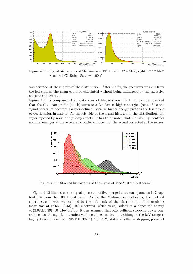
hSpec_timecut1Entries 458175

Mean 1.201e+05

Std Dev 6.914e+04 / ndf 2χ 136 / 36

Constant 16.6± 4471

Mean 1.229e+02± 1.516e+05 Sigma 2.472e+02± 2.473e+04

electrons)3Signal (1050 100 150 200 250 300 350 400 450 500

310×0

500

1000

1500

2000

2500

3000

3500

4000

4500hSpec_timecut1

Entries 458175

Mean 1.201e+05

Std Dev 6.914e+04 / ndf 2χ 136 / 36

Constant 16.6± 4471

Mean 1.229e+02± 1.516e+05 Sigma 2.472e+02± 2.473e+04

Spectrum with Time cut [0 , 100]

hSpec_timecut1Entries 211515Mean 5.068e+04Std Dev 3.397e+04

/ ndf 2χ 641.1 / 140Constant 1.456e+02± 3.478e+04 MPV 9.520e+01± 3.619e+04 Sigma 25.5± 6493

electrons)3Signal (100 50 100 150 200 250

310×0

1000

2000

3000

4000

5000

6000hSpec_timecut1

Entries 211515Mean 5.068e+04Std Dev 3.397e+04

/ ndf 2χ 641.1 / 140Constant 1.456e+02± 3.478e+04 MPV 9.520e+01± 3.619e+04 Sigma 25.5± 6493

Spectrum with Time cut [0 , 100]

Figure 4.10.: Signal histograms of MedAustron TB 1. Left: 62.4 MeV, right: 252.7 MeVSensor: IFX Baby, Ubias = -100V

was oriented at these parts of the distribution. After the fit, the spectrum was cut fromthe left side, so the mean could be calculated without being influenced by the excessivenoise at the left tail.Figure 4.11 is composed of all data runs of MedAustron TB 1. It can be observedthat the Gaussian profile (black) turns to a Landau at higher energies (red). Also thesignal spectrum becomes sharper defined, because higher energy protons are less proneto deceleration in matter. At the left side of the signal histogram, the distributions aresuperimposed by noise and pile-up effects. It has to be noted that the labeling identifiesnominal energies at the accelerator outlet window, not the actual corrected at the sensor.

Figure 4.11.: Stacked histograms of the signal of MedAustron testbeam 1.

Figure 4.12 illustrates the signal spectrum of five merged data runs (same as in Chap-ter4.1.3) from the DESY testbeam. As for the Medaustron testbeams, the methodof truncated mean was applied to the left flank of the distribution. The resultingmean was at (2.65 ± 0.43) · 104 electrons, which is equivalent to a deposited energyof (2.08± 0.39) · 104 MeVcm2/g. It was assumed that only collision stopping power con-tributed to the signal, not radiative losses, because bremsstrahlung in the keV range ishighly forward oriented. NIST ESTAR (Figure2.2) states a collision stopping power of

58

2.24MeVcm2/g for 5.6GeV electrons (NIST ESTAR[15], 2018/03).However, the usage of truncated mean is problematic because the mean value is notrobust to signal cuts and should be used with caution.

Entries 665561

Mean 2.495e+04

/ ndf 2χ 1.595e+05 / 386

Constant 2.91e+02± 1.33e+05

Sigma 3.9± 2271

electrons)3Signal (100 20 40 60 80 100 120 140

310×0

5000

10000

15000

20000

25000Entries 665561

Mean 2.495e+04

/ ndf 2χ 1.595e+05 / 386

Constant 2.91e+02± 1.33e+05

Sigma 3.9± 2271

Spectrum with Time cut [0 , 100]

Figure 4.12.: Signal histogram of five merged runs at DESY.Sensor: IFX CenterBias, Ubias = -100V, 5.6GeV electrons

4.2. Energy correction of MedAustron dataAs seen in Figures 4.10 and 4.11, the energy profile of the lower proton energies did notfollow a Landau distribution any longer. The mean ranges in silicon for these energyranges was short enough for the detector to act as a thick absorber, so the resultingprofile was Gaussian. As seen in Figure 4.13, stopping power of air and plastic at energyranges used at MedAustron should not be neglected. Due to the scintillator thicknessof 1 cm, it was expected to lose approximately 10MeV at the lowest energy of 62.4MeV.The stopping power of air is three magnitudes lower, but the penetrated material thick-ness was two magnitudes higher (60 cm). To encounter this issue, the setup of the secondtestbeam was changed (see Chapter 3.6).To quantify energy losses, the simulation tool SRIM ("Stopping and Range of Ions

in Matter", Ziegler 2010[29]) was used. Material budget was modeled as consecutive,homogeneous layers. Because PVT and PVC have similar and non-negligible stoppingpowers, the light shielding tape was also taken into account.At TB 1, the overall presumed material budget was 50µm polyimide (for the acceleratorsoutlet window), 60 cm air (50 cm between beam outlet and scintillator; 10 cm betweenscintillator and DUT), 1 cm PVT (scintillator) and 1mm PVC (light shieldings of scin-tillators and DUT). Figure 4.14 illustrates the corresponding material layers. To balanceprecision and run time, 1000 protons per energy run were simulated. It has to be notedthat layers of similar composition were merged to single layers, because the number oflayers was limited to 5 in SRIM. For a better precision, advanced simulation softwarelike Geant4 is recommended.At TB 2, the material budget was 50µm polyimide (same as before), 25 cm air and

59

1 0 1 0 0 1 0 0 00 , 0 0 1

0 , 0 1

0 , 1

1

1 0

1 0 0

stopp

ing po

wer (M

eV/cm

)

e n e r g y ( M e V )

P V T s c i n t i l l a t o r a i r

Figure 4.13.: Total stopping power for protons in polyvinyltoluene-based plastic scintil-lators and air (NIST PSTAR[15], 2018/02)

Figure 4.14.: Material budget for simulation of MedAustron TB 1 energy loss

200 µm PVC. Figure 4.15 represents the material layers. 2000 protons per run weresimulated.The resulting runs were averaged per energy, and standard deviation was calculated.

Tables 4.1 and 4.2 demonstrate the outcome of the simulations. It makes clear that interms of energy loss the TB 2 setup is superior to the TB 1, especially at low energies.The extra material layers before the sensor also lead to additional widening of the beamthrough scattering.

60

Figure 4.15.: Material budget for simulation of MedAustron TB 2 energy loss

nominal E E loss E at sensor loss(MeV) (MeV) (MeV) (%)

62.4 28.7± 0.92 33.7± 0.92 46.0± 1.597.4 17.8± 0.53 79.6± 0.53 18.3± 0.5

148.2 12.6± 0.54 135.6± 0.54 8.5± 0.4175.3 11.1± 0.56 164.2± 0.56 6.3± 0.3198.0 10.2± 0.55 187.8± 0.55 5.2± 0.3252.7 8.7± 0.59 244.0± 0.59 3.5± 0.2

Table 4.1.: Results of SRIM simulation for energy loss before sensor at MedAustron TB 1

nominal E E loss E at sensor loss(MeV) (MeV) (MeV) (%)

62.4 6.1± 0.25 56.3± 0.25 9.8± 0.383.0 4.8± 0.26 78.2± 0.26 5.8± 0.2100.4 4.2± 0.27 96.2± 0.27 4.1± 0.2145.4 3.2± 0.30 142.2± 0.30 2.2± 0.1175.3 2.8± 0.31 172.5± 0.31 1.6± 0.1194.3 2.6± 0.33 191.7± 0.33 1.3± 0.1252.7 2.2± 0.38 250.5± 0.38 0.9± 0.1

Table 4.2.: Results of SRIM simulation for energy loss before sensor at MedAustron TB 2

4.3. Stopping power determinationDue to the high noise contribution at low energy deposition scales (see Figure 4.8), fittingwas focused at the right hand side of the Landau distribution. This led to the possibilityfor estimation of the left hand flank, to further distinguish it from noise. Multiplyingthe mean number of electrons with ionization energy (3.65 eV for silicon) gave the meandeposited energies. Dividing it per the active sensor thickness (thickness of the fulldepletion zone; 200 µm for the Infineon sensors used of the MedAustron testbeams)represents the mean energy deposition dE

dx , same as the outcome of the Bethe-Blochformula. Dividing it by the mass density of silicon (2.329 g cm-3) delivered the stopping

61

3 0 6 0 9 0 1 2 0 1 5 0 1 8 0 2 1 0 2 4 0 2 7 0 3 0 01

1 0

stopp

ing po

wer (M

eV*cm

²/g)

e n e r g y ( M e V )

M e d A u s t r o n T B 1 M e d A u s t r o n T B 2 N I S T P S T A R

Figure 4.16.: Stopping power with energy correction of MedAustron TBs, compared toNIST PSTAR data[15]

power per density (see Figure 4.16).It is assumed that the excessive stopping power of MedAustron TB 1 (red dots) islinked to pile-up effectse and occupancy (see Chapter 4.1.3). At these high particlerates, observation of the display of the bias voltage SMU via a webcam revealed thatthe compliance indicator LED flashed up. This lead to the conclusion that bias voltagedrops during the spills reduced charge generation (by reducing the sensor’s active volumethrough depletion zone shrink) and current flow (by reducing the electrical field). Theseeffects were expected to partly compensate the raised energy deposition by multiple hits.The effect of bias voltage drop and subsequently reduced current pulses should be moresevere at lower particle energies because of higher stopping power. This conforms to theleft red dot in 4.16.At TB 2 (green dots), the reduced particle rate didn’t cause occupancy and bias voltagedrops, so the stopping power showed good comparability to NIST PSTAR data[15].The error of calculated stopping power is dominated by the fitting procedure. Pile-up

eoverlapping pulses increase total pulse area per hit

62

effects, material in front of the sensor (both widened the Landau/Gauss distribution) andnoise contribution at low energies impeded the identification of spectral peaks and flanks.Due to the tight time budget of 6 h of beam time per shift at MedAustron testbeams,it was difficult to obtain sufficient counts for adequate statistics at lower particle rates(TB 2). However, due to the method of truncated mean and broad cuts, peak and flankidentification was possible and contributed to a lower overall error compared to TB 1.The DAQ quantization error was considered to be negligible.The stopping power error is mainly determined by application of the fitting parameters,the energy error is dominated by simulation simplification and precision, as well asgeometrical uncertainties like layer thickness and distances.

4.4. Sensor current at high rate proton beamOne of the data runs of MedAustron TB 2 was taken at high particle rate (109/s) at lowestenergy (62.4MeV) to maximize electron-hole pairs and therefore current consumption.Figure 4.17 shows that the currents reached up to 6.5 µA, which was 50 times IFX Irrad’sidle current of 130 nA, exceeding typical compliance thresholds. This result confirmedthe hypothesis that in TB 1 compliance of the bias voltage supply was reached at eachspill, explaining the suppression of high signal pulses due to the effective bias voltage inthe compliance situation.

0 2 0 0 4 0 0 6 0 0 8 0 0 1 0 0 00

1

2

3

4

5

6

7

curre

nt (uA

)

t i m e ( s )Figure 4.17.: Current consumption over time of IFX Irrad used at MedAustron TB2

63

5. Conclusions and Suggestions

Within the framework of this diploma thesis, the proton beam of MedAustron was usedto test silicon sensors for first time. During the first testbeam (TB 1) it was observedthat the compliance indicator LED of the SMU for the power supply flashed up duringthe spills. After the first testbeam, results of the analysis showed that high particle ratesup to 1010/s lead to pile-up effects and occupancy. Measured stopping power thereforewas exaggerated, although it was partly compensated by the compliance of the powersupply SMU, leading to a bias voltage drop which decreased charge generation and pulsecurrents.To quantify the ALiBaVa’s maximum processable data rate, radioactive source tests re-vealed that the system’s maximum rate is about 600Hz in average, but allowing burstsin the lower kHz range. This is far below particle rates at TB 1.At low proton energies (62MeV), the Gaussian beam profile showed an intense wideningthrough scattering in the first scintillator and the passage through air.Before the second testbeam, MedAustron’s staff prepared, installed and tested particlerate reduction systems. At MedAustron TB 2, the setup was modified by installing alltrigger scintillators after the silicon sensor to reduce energy loss of the beam. In addi-tion, the elements were placed together as tight as possible and close to the beam outletwindow. To monitor current consumption of the strip sensor, the bias supply SMU’sdata was read out by USB.At TB 2, the bias supply SMU showed no indications of compliance, providing a stablevoltage supply. In terms of measured stopping power, the setup of TB 2 was far superiorto its predecessor. The results showed excellent conformity to reference data. Clusteranalysis confirmed the reduction of occupancies at reduced particle rates of 105/s. Forextended cluster analysis, one has to examine the behavior over the full sensor size.However, it will be necessary to modify the analysis algorithm to extend the search.Between TB 1 and TB 2, a testbeam together with Karlsruhe Institute of Technology(KIT) was conducted at DESY. Using the electron beam (5.6GeV) from DESY II, sixsensors were tested (two from HEPHY and four from KIT). Particle rates were at ap-proximately 200Hz, low enough to be continuously processed by the ALiBaVa system.All testbeams (MedAustron and DESY) exhibit high noise levels at small signal ranges,whereas this problem did not show up at the preparatory tests at HEPHY. It is assumedthat this noise was caused by extrinsic factors, like focusing magnets, vacuum pumpsand other control devices of the beam outlet. Modeling this noise behavior via an expo-nential function and subtracting it from the signal failed, so it was difficult to distinguishbetween noise and signal.To circumvent the problem of noise at the lower spectrum, the method of truncatedmean was successful for determining the mean value. However, the usage of this tech-

64

nique is problematic because the mean value is not robust to signal cuts. Due to thisfact, verifications via Landau/Gauss fits are recommended.Prospective testbeams require extensive preparations in terms of functionality tests andstandardization. It is recommended to simulate the setup in advance to identify designflaws. For achieving better energy resolution in future, well-defined particle rate controlis essential, as well as monitoring the current consumption of the sensor to avoid biasvoltage drops. If there is a demand for low-energy beam testing, it is essential to ana-lyze the non-linear gain behavior in the upper energy deposition range of the ALiBaVasystem and extending the system’s algorithm by adding an ADC-to-electrons-mapping.To make the setup resistant against RF interference, single-point grounding via copperstrips prevents ground loops. It is proposed to add additional grounded shielding to theelectrical components to further enhance protection against electromagnetic coupling.Maybe it will be possible to find an appropriate model to quantify electronic noise con-tribution to improve SNR. To measure beam profiles, the small sensor used at TB 2 wasway too slim to cover the full beam distribution. Even the larger sensor of TB 1 wasnot sufficient, so larger strip sensors may be used for this task.At MedAustron, short night shifts of 6 hours of beam time made troubleshooting diffi-cult. For the next testbeams, it is suggested to conduct two or more consecutive shiftsat weekends to expand active beam time, generating more data runs and improving timeefficiency.

65

Bibliography

[1] CERN, Organisation européenne pour la recherche nucléaire (2017), URL http://home.cern/about/updates/2015/04/proton-beams-are-back-lhc.

[2] ILC-Collaboration, ILC Technical Design Report (2018), URL http://www.linearcollider.org/.

[3] CERN, A Roadmap for HEP Software and Computing RD for the 2020s, Tech. Rep.HSF-CWP-2017-001 (2017), URL http://cds.cern.ch/record/2298968.

[4] CMS-Collaboration, The CMS experiment at the CERN LHC, CERN-CMS, URLhttps://cds.cern.ch/record/1129810.

[5] Lippmann, C., Particle identification, Nucl. Instrum. Meth., A666 (2012) 148–172.

[6] Wells, P. S., The upgraded ATLAS and CMS detectors and their physics capa-bilities, Philosophical Transactions of the Royal Society of London A: Mathe-matical, Physical and Engineering Sciences, 373(2032), ISSN 1364-503X, URLhttp://rsta.royalsocietypublishing.org/content/373/2032/20140046.

[7] CMS-Collaboration, CMS Technical Design Report for the Pixel Detector Upgrade,CERN-CMS, URL http://cds.cern.ch/record/1481838.

[8] Friedl, M., The CMS Silicon Strip Tracker and its Electronic Readout, Dissertation,Technische Universitäet Wien (2011), URL http://www.hephy.at/user/friedl/diss/html/disshtml.html.

[9] CMS-Collaboration, Observation of a new boson at a mass of 125 GeV with theCMS experiment at the LHC, CERN-CMS, URL https://doi.org/10.1016/j.physletb.2012.08.021.

[10] CMS-Collaboration, Technical Proposal for the Phase-II Upgrade of the CompactMuon Solenoid, CERN-CMS, URL https://cds.cern.ch/record/2020886.

[11] CMS-Collaboration, The Phase-2 Upgrade of the CMS Tracker, CERN-CMS, URLhttps://cds.cern.ch/record/2272264.

[12] Schreiner, T., Physics Meets Medicine (2018).

[13] DESY, Deutsches Elektronen-Synchrotron: DESY II (2018), URL http://desy2.desy.de/.

66

[14] Kolanoski, H. and Wermes, N., Teilchendetektoren, Grundlagen und Anwendungen,Springer Spektrum (2016), ISBN 978-3-662-45349-0.

[15] NIST, Physical Measurements Laboratory (2017), URL https://physics.nist.gov/PhysRefData/Star/Text/intro.html.

[16] PDG, Passage of particles through matter (2007), URL http://pdg.lbl.gov/2009/reviews/rpp2009-rev-passage-particles-matter.pdf.

[17] InterAction-Collaboration, Quantum Diaries, URL https://www.quantumdiaries.org/.

[18] Ramo, S., Currents Induced by Electron Motion, Proceedings of the IRE, 27(9)(1939) 584–585, ISSN 0096-8390.

[19] Spieler, H., Semiconductor Detector Systems, Oxford Science Publications (2005),ISBN 978-0-19-852784-8.

[20] Grupen, C. and Buvat, I., Handbook of Particle Detection and Imaging, SpringerReference (2012), ISBN 978-3-642-13270-4.

[21] Hinger, V., Charge Sharing Studies of Silicon Strip Sensors for the CMS Phase IIUpgrade, Diploma thesis, Technische Universität Wien (2017).

[22] König, A., Electrical Characterisation and Aging Studies of Silicon Strip Sensors,Master thesis, Universität Wien (2014).

[23] Löchner, S. and Schmelling, M., The Beetle Reference Manual, LHCb Electronics.

[24] ALiBaVa, Alibava user’s manual (2018), URL https://www.alibavasystems.com/.

[25] IAEA, Nuclear structure and decay data (2018), URL https://www-nds.iaea.org/relnsd/vcharthtml/VChartHTML.html.

[26] Badano, L. T. and Rossi, S. C., Characteristics of a Betatron Core for Extractionin a Proton-Ion Medical Synchrotron, THPS048.

[27] Borburgh, J. and Kramer, T., Design of Electrostatic Septa and Fast Deflector forMedAustron, THPS048.

[28] DESY, Deutsches Elektronen-Synchrotron: Telescopes (2018), URL https://telescopes.desy.de/.

[29] Ziegler, J. F., Ziegler, M. D. and Biersack, J. P., SRIM - The stopping and rangeof ions in matter (2010), Nuclear Instruments and Methods in Physics Research B,268 (2010) 1818–1823, URL http://www.srim.org/.

67

List of Figures

1.1. Accelerators and detectors of the Large Hadron Collider . . . . . . . . . . 91.2. Run and shutdown schedule of the LHC . . . . . . . . . . . . . . . . . . . 91.3. Compact Muon Solenoid . . . . . . . . . . . . . . . . . . . . . . . . . . . . 101.4. Particle signatures in CMS . . . . . . . . . . . . . . . . . . . . . . . . . . 111.5. Inner pixel system . . . . . . . . . . . . . . . . . . . . . . . . . . . . . . . 121.6. Sketch of the prospective Outer Tracker layout of Phase-II . . . . . . . . . 151.7. Layout of the MedAustron accelerator . . . . . . . . . . . . . . . . . . . . 151.8. Accelerators at DESY . . . . . . . . . . . . . . . . . . . . . . . . . . . . . 171.9. DESY II synchrotron with test beam sites . . . . . . . . . . . . . . . . . . 18

2.1. Bremsstrahlung radiated from an electron . . . . . . . . . . . . . . . . . . 202.2. Mass stopping power for electrons in silicon . . . . . . . . . . . . . . . . . 212.3. Mass stopping power for protons in silicon . . . . . . . . . . . . . . . . . . 232.4. Relative dose distribution for different particles in water . . . . . . . . . . 242.5. Energy and angular distribution ofd-electrons . . . . . . . . . . . . . . . . 242.6. Gaussian profile for low energy antiprotons . . . . . . . . . . . . . . . . . 252.7. Landau distribution . . . . . . . . . . . . . . . . . . . . . . . . . . . . . . 262.8. Schematic view on a scintillation detector system . . . . . . . . . . . . . . 272.9. Principle of a constant fraction discriminator . . . . . . . . . . . . . . . . 292.10. Mobility of charge carriers in silicon at 300K . . . . . . . . . . . . . . . . 312.11. Drift and diffusion at a p-n junction . . . . . . . . . . . . . . . . . . . . . 322.12. Detector diode and preamplifier . . . . . . . . . . . . . . . . . . . . . . . . 342.13. Schematic view of a strip sensor . . . . . . . . . . . . . . . . . . . . . . . . 35

3.1. Telescope setup for testbeams . . . . . . . . . . . . . . . . . . . . . . . . . 363.2. Sketch of the ALiBaVa-System . . . . . . . . . . . . . . . . . . . . . . . . 383.3. Screenshot of the ALiBaVa GUI . . . . . . . . . . . . . . . . . . . . . . . 393.4. Bad tape shielding of scintillator 1 . . . . . . . . . . . . . . . . . . . . . . 413.5. Coordinate system of the scintillator tests . . . . . . . . . . . . . . . . . . 423.6. Dark rate versus radiation source rate for both scintillators . . . . . . . . 423.7. Geometry scans of scintillators used at MedAustron TB 1 . . . . . . . . . 433.8. Count rates at additional layers of tape . . . . . . . . . . . . . . . . . . . 433.9. I-V characteristics of the sensors used at MedAustron testbeams . . . . . 443.10. Histogram of the signal of a preparatory test run using the 90Sr source . . 453.11. Signal histogram of laser tests at HEPHY . . . . . . . . . . . . . . . . . . 463.12. DAQ, triggering and power supply at MedAustron TB 1 . . . . . . . . . . 483.13. DAQ, triggering and power supply at MedAustron TB 2 . . . . . . . . . . 49

68

3.14. DAQ and triggering at DESY . . . . . . . . . . . . . . . . . . . . . . . . . 51

4.1. Noise spectra of HEPHY preparatory tests and MedAustron TB 1 . . . . 524.2. Noise per channel of MedAustron TB 2 . . . . . . . . . . . . . . . . . . . 534.3. Gain scan of MedAustron TB 2 . . . . . . . . . . . . . . . . . . . . . . . . 534.4. Cluster sizes of MedAustron TB 2 at different energies and particle rates . 544.5. Number of clusters per event of MedAustron TB 2 at different energies

and particle rates . . . . . . . . . . . . . . . . . . . . . . . . . . . . . . . . 554.6. Comparison of cluster sizes of all testbeams . . . . . . . . . . . . . . . . . 564.7. Comparison of clusters per event of all testbeams . . . . . . . . . . . . . . 564.8. Hitmaps of MedAustron TB 1 . . . . . . . . . . . . . . . . . . . . . . . . . 564.9. Comparison of beam profiles of MedAustron testbeam 1 . . . . . . . . . . 574.10. Signal histograms of of MedAustron TB 1 . . . . . . . . . . . . . . . . . . 584.11. Stacked histograms of the signal of MedAustron testbeam 1 . . . . . . . . 584.12. Signal histogram of five merged runs at DESY . . . . . . . . . . . . . . . 594.13. Stopping power in PVT-based scintillators and air . . . . . . . . . . . . . 604.14. Material budget for simulation of MedAustron TB 1 energy loss . . . . . . 604.15. Material budget for simulation of MedAustron TB 2 energy loss . . . . . . 614.16. Stopping power with energy correction of MedAustron TBs . . . . . . . . 624.17. Current consumption over time of the sensor used at MedAustron TB2 . . 63

List of Tables

1.1. LHC parameters . . . . . . . . . . . . . . . . . . . . . . . . . . . . . . . . 81.2. Beam parameters of the MedAustron synchrotron . . . . . . . . . . . . . . 161.3. DESY II parameters . . . . . . . . . . . . . . . . . . . . . . . . . . . . . . 17

2.1. Parameters of the Bethe-Bloch equation . . . . . . . . . . . . . . . . . . . 22

3.1. Parameters of ulitized strip sensors . . . . . . . . . . . . . . . . . . . . . . 443.2. Parameters of the laser system . . . . . . . . . . . . . . . . . . . . . . . . 463.3. Overview of usable data runs at MedAustron TB 1 . . . . . . . . . . . . . 473.4. Overview of usable data runs at MedAustron TB 2 . . . . . . . . . . . . . 493.5. Used strip sensors at DESY . . . . . . . . . . . . . . . . . . . . . . . . . . 51

4.1. Energy loss before sensor at MedAustron TB 1 . . . . . . . . . . . . . . . 614.2. Energy loss before sensor at MedAustron TB 2 . . . . . . . . . . . . . . . 61

69

Glossary

ADC analog digital converter. 38–40, 53, 54, 65

APD avalanche photodiode. 27

CMS Compact Muon Solenoid. 7, 10–13, 34

CSDA continuous slowing down approximation. 22

DAQ data acquisition. 36, 37, 47–51, 63

DESY Deutsches Elektronen-Synchrotron. 4, 6, 17, 37, 44, 50, 51, 55, 58, 59, 64

DUT device under test. 37, 38, 47, 48, 50, 59

FWHM full width at half maximum. 16, 17, 47

LHC Large Hadron Collider. 7–10, 36, 38, 68

MIP minimal ionizing particle. 46, 54

MPV most probable value. 25

PDF probability density function. 25, 26

PMMA polymethyl methacrylate. 37

PMT photomultiplier tube. 13, 27, 28, 36, 47

PVC polyvinyl chloride. 57, 59, 60

PVT polyvinyl toluene. 37, 57, 59

SiPM silicon photomultiplier. 27

SNR signal-to-noise ratio. 40, 45, 65

TB testbeam. 6, 15, 29, 42, 43, 47–50, 52–65, 68, 69

TLU trigger logic unit. 37

70

A. Appendix

A.1. Software used for this thesis• ALiBaVa-GUI: https://www.alibavasystems.com/

• Atom: https://atom.io/

• DESY software environment: https://telescopes.desy.de/User_manual

• SRIM-2013: http://www.srim.org/

• Web Plot Digitizer: https://automeris.io/WebPlotDigitizer/

• yEd Graph Editor: https://www.yworks.com/products/yed

A.2. Important hints for the usage of the ALiBaVa system• Is the beam hitting all planes? Check the online Hitmap. Is there currently a spill?

• Is the sensor’s power supply on?

• A crossed flat band cable between mother- and daughterboard is needed.

• Is the configuration of the Beetle chip correct? Is the latency correct? Pulse-shaping has to be activated!

• The calibration run only works if the latency is set to 128. After this, set immedi-ately to the value appropriate for the triggering system.

• Don’t forget to do frequent pedestal runs!

• Don’t forget to click on "LogData"! Otherwise the data would not be saved to afile! Good practice: Save pedestals as .dat AND .ped files, via both GUI-Buttons.The .dat directly via "LogData" and the .ped via File → Save Pedestals.

A.3. Work inputFor all work besides writing, a total of 1113 working hours were applied. Auxiliary work(pre-beam-tests, administrative work, planning and organizing, meetings etc.) took 195hours. Data aquisition and analysis took 454 hours for the two MedAustron testbeams,and 464 hours for the DESY testbeam.Writing this diploma thesis was completed in 310 hours.

71