Advanced Corporate

Finance

(GEST S 410)

1. Introduction

Professor Kim Oosterlinck

E-mail: koosterl@ulb.ac.be

|2

Course Outline (1/4)

• Theory (24h) + Exercises (12h) + Textbooks and

references

• Material available on

• http://homepages.ulb.ac.be/~koosterl/

• Prerequisites: Accounting, Microeconomics and

Finance 101

• => Familiar with PV, Bonds and Stocks Valuation,

NPV, IRR rules, portfolio theory, CAPM and option

pricing (binomial model)

|3

Course Outline (2/4)

Reference books:

David Hillier, Stephen Ross, Jeffrey Jaffe, Randolph

Westerfield, (2013), Corporate Finance European edition,

2nd edition.

Berk, J. and P. DeMarzo, (2013), Corporate Finance, 3rd ed.

Pearson,

Bodie Zvi, Kane Alex, Marcus Alan J., (2011), Investments and

Portfolio Management, Global Edition, McGraw Hill,

Brealey, R., Myers, S. and Allen, F. (2008), Principle of

Corporate Finance, 9th ed., McGraw-Hill.

Course Outline (3/4)

• Second course in finance. Objectives, understand:

�How to move from accounting to cash-flows

�The impact of capital structure on investment

decisions

�The Value of the Firm (Modigliani-Miller)

� Optimal capital structure

�Raising Capital and Going Public (IPO, SEO)

�Mergers and Acquisitions

�Risky Debt

|4

Course Outline (4/4)

• Exam

– Theory and Exercises

– No help allowed…

– The Course is in ENGLISH => no dictionary, you

should have a sufficiently good knowledge NOW

– Exam is HARD be precise when answering

– Erasmus no exam outside the normal sessions

|5

|6

Roadmap

1. Introduction and Review of supposedly known concepts

2. From Accounting to Cash Flows

3. Capital Structure

4. Project valuation using the wacc

5. Financial Options

6. Real Options

7. Market efficiency

8. Raising capital and going public

9. Long Term Bonds

10. Alternative Investments

|7

Beware, Beware, Beware

• This session will provide a short wrap-up of what I

believe should be known…

• If you never had a finance class before: WORK

• To help you here are the hillier et al.(2013) chapters I

assume you have seen BEFORE this class:

• At least chapters: 1,2, 4, 5, 6, 7, 10 and 22

• If not it is up to YOU to make up for this

|8

A short review

• Financial valuation most of the time relies on the

discounting concept

• Decisions to invest or not in a project are then made

based on the NPV rule (invest if NPV > 0). Even

though other methods exist (IRR, Payback etc) they

do not always yield a proper result => stick to NPV!!!

• Choosing the proper interest rate to use is not easy

(more on this later). Besides one must take into

account compounding intervals

|9

A short review

• One may also wish to benefit from shortcut

formulas to compute PV

• Discounting future cash flows is also at the basis of

bonds and equity valuation

• The discount rate should take risk into account

• Capital Asset Pricing Model (CAPM)

|10

Discounting: Time value of Money

0 1

C (€100)

?

C (€100)

?

Future value

Present value

Case 1

Case 2

( )100 1 r= × +

( ) 1

100100

1DF

r= × =

+

Capitalizing

Discounting

With Cash Flows

|11title |11

time

0 1

Future value

Present value

Case 1

Case 2

2 … n

C (€100)

?

CF (€100)

?

( )0 1C r× + ( )

( )0 1

1

C r

r

× +

× +

( )

( )0 1

1

...

C r

r

× +

× +

×

( )0 1n

C r× +

( )1

n

n

C

r+ ( )1

1

nC

r+

n-1

( ) ( )1

1...

11

nC

rr× ×

++( )1

1

1n

n

Cr−

×+

∏ ( )2

1

1n

n

Cr−

×+

∏

|12

The discount factor

title |12

• How much would an investor pay today to receive € Ct in t years given market

interest rate rt?

– We know that 1 €0 → (1+rt)t €t

– Hence PV × (1+rt)t = Ct → PV = Ct /(1+rt)

t = Ct × DFt

• The process of calculating the present value of future cash flows is called

discounting.

• The present value of a future cash flow is obtained by multiplying this cash

flow by a discount factor (or present value factor) DFt

• The general formula for the t-year discount factor is:

t

t

tr

DF)1(

1

+=

Net Present Value

• Decide whether it is worth investing in a project

• Rule => it should bring money. To compare the cash flows arriving at ≠

dates => discount the cash flows

• Cash flows: C0 C1 C2 … Ct … CT

• t-year discount factor: DFt = 1/(1+r)t

• NPV = C0 + C1 DF1 + … + Ct DFt + … + CT DFT

• Usually C0 < 0 since it often represents the investment made for the project

|13

Example…

|14

• Suppose r = 10%

• In this case the investment is worth undertaking

• NB: an alternative method could have been to compute the Net Future Value

(NFV)

t 0 1 2 3

Cash flow -100 30 60 40

Discount Factor 1 0.9091 0.8264 0.7513

PresentValue -100.0 27.3 49.6 30.1

NPV 6.9

Internal Rate of Return

• The Internal Rate of Return is the discount rate such that the NPV is equal

to zero.

|15

-25.0

-20.0

-15.0

-10.0

-5.0

0.0

5.0

10.0

15.0

20.0

25.0

0% 5% 10% 15% 20% 25% 30% 35% 40% 45% 50%

Discount rate

Ne

t P

re

se

nt

Va

lue

IRR

Internal Rate of Return

• In a multiple period setting• Reinvestment assumption: the IRR calculation

assumes that all future cash flows are reinvested at the IRR

• Disadvantages:– Does not distinguish between investing and

financing– IRR may not exist or there may be multiple IRR – Problems with mutually exclusive investments

• Advantages:– Easy to understand and communicate

|16

Compounding Interval

• Up to now, interest paid annually

• If n payments per year, compounded value after 1 year :

• Example: Monthly payment :

– r = 12%, n = 12

– Compounded value after 1 year : (1 + 0.12/12)12= 1.1268

– Effective Annual Interest Rate : 12.68%

• Continuous compounding:

– [1+(r/n)]n→ern (e= 2.7183)

– Example : r = 12% e12 = 1.1275

– Effective Annual Interest Rate : 12.75%

|17

Shortcut Formulas…

|18title |18

• Constant perpetuity: Ct = C for all t

• Growing perpetuity: Ct = Ct-1(1+g)

r>g t = 1 to ∞

• Constant annuity: Ct=C t=1 to T

• Growing annuity: Ct = Ct-1(1+g)

t = 1 to T

r

CPV =

gr

CPV

−= 1

))1(

11(

Trr

CPV

+−=

))1(

)1(1(1

T

T

r

g

gr

CPV

+

+−

−=

Bond valuation

• Zero-Coupon � one bullet payment at maturity T

• Level coupon bond, paying a yearly coupon C

• With A the annuity factor

• NB: Inverse relationship between interest rate r and Bond Price!

|19

TrPV

)1(

1

+=

T

T

rTTdAC

rr

C

r

C

r

CP ×+×=

++

+++

++

+= 100

)1(

100

)1(...

)1(1 20

Stock (Equity) valuation

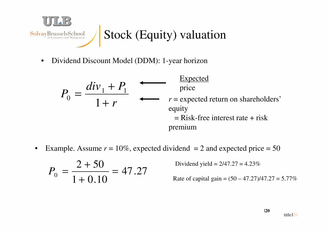
• Dividend Discount Model (DDM): 1-year horizon

|20title |20

• Example. Assume r = 10%, expected dividend = 2 and expected price = 50

r

PdivP

+

+=

1

110

27.4710.01

5020 =

+

+=P

Expected

price

r = expected return on shareholders’

equity

= Risk-free interest rate + risk

premium

Dividend yield = 2/47.27 = 4.23%

Rate of capital gain = (50 – 47.27)/47.27 = 5.77%

DDM: where does the expected

stock price come from?

|21title |21

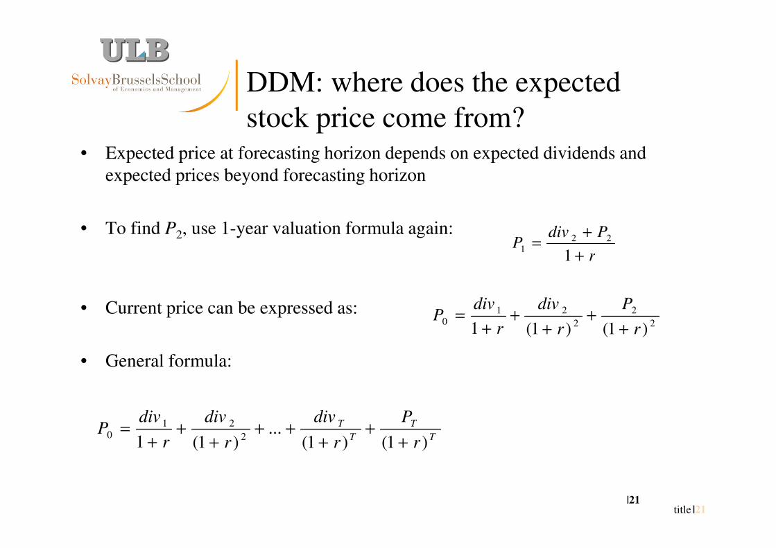
• Expected price at forecasting horizon depends on expected dividends and

expected prices beyond forecasting horizon

• To find P2, use 1-year valuation formula again:

• Current price can be expressed as:

• General formula:

r

PdivP

+

+=

1

221

2

2

2

210

)1()1(1 r

P

r

div

r

divP

++

++

+=

T

T

T

T

r

P

r

div

r

div

r

divP

)1()1(...

)1(1 2

210

++

+++

++

+=

DDM - general formula

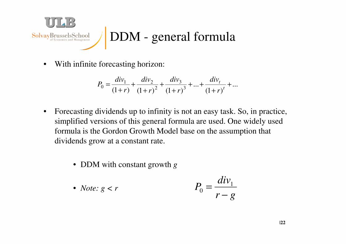
• With infinite forecasting horizon:

• Forecasting dividends up to infinity is not an easy task. So, in practice,

simplified versions of this general formula are used. One widely used

formula is the Gordon Growth Model base on the assumption that

dividends grow at a constant rate.

• DDM with constant growth g

• Note: g < r

|22

...)1(

...)1()1()1( 3

3

2

210 +

+++

++

++

+=

t

t

r

div

r

div

r

div

r

divP

gr

divP

−= 1

0

Risk-Return and diversification

• Risk linked to return

• Benefits from diversification, let us consider a portfolio of two stocks

(A,B)

• Characteristics:

– Expected returns :

– Standard deviations :

– Covariance :

• Portfolio: defined by fractions invested in each stock XA , XB

XA+ XB= 1

• Expected return on portfolio:

• Variance of the portfolio's return:

|23

BA RR ,

BA σσ ,

BAABAB σσρσ =

BBAAP RXRXR +=

22222 2 BBABBAAAP XXXX σσσσ ++=

Covariance and correlation

• Statistical measures of the degree to which random variables move together

• Covariance

• Like variance figure, the covariance is in squared deviation units.

• Not too friendly ...

• Correlation

• Covariance divided by product of standard deviations

• Covariance and correlation have the same sign

– Positive : variables are positively correlated

– Zero : variables are independent

– Negative : variables are negatively correlated

• The correlation is always between –1 and + 1

|24

)])([(),cov( BBAABAAB RRRRERR −−==σ

BA

BABAAB

RRCovRRCorr

σσρ

),(),( ==

Portfolio with many assets

• Portfolio composition :

• (X1, X2, ... , Xi, ... , XN)

• X1 + X2 + ... + Xi + ... + XN = 1

• Expected return:

• Risk:

• Note:

• N terms for variances

• N(N-1) terms for covariances

• Covariances dominate

|25

NNP RXRXRXR +++= ...2211

∑∑ ∑∑∑≠

=+=i ij i j

ijjiijjij

j

jP XXXXX σσσσ 222

Covariance domination…

|26

Var Cov Cov Cov Cov

Cov Var Cov Cov Cov

Cov Cov Var Cov Cov

Cov Cov Cov Var Cov

Cov Cov Cov Cov Var

Equally weighted portfolio

• Consider the risk of an equally weighted portfolio of N "identical« stocks:

• Equally weighted:

• Variance of portfolio:

• If we increase the number of securities ?:

• Variance of portfolio:

|27

NX j

1=

cov)1

1(1 22

NNP −+= σσ

∞→

→

N

P cov2σ

cov),(,, === jijj RRCovRR σσ

In practice

|28title |28

Diversification gains already close to maximum with n = 20

n

σP

Diversification limit

20

Systematic

risk

Unsystematic risk

Risk and CAPM

• Discount rate should take risk into account

• Concept of opportunity cost

• Risk usually measured as the standard deviation of returns

• Part of the risk may be reduced thanks to diversification

• The market only rewards the risk which cannot be diversified

• Capital-Asset Pricing Model (CAPM)

• with

|29

β×−+= )( FMF RRRR

22 )(

),(

M

iM

M

Mii

R

RRCov

σ

σ

σβ ==

This course…

• Many questions remain unanswered

=> How do we determine the Cash Flows to Discount?

⇒CAPM provides some insights regarding the discount rate but

how is it affected by the capital structure (% debts versus

equity)?

⇒ Is there such a thing as an optimal capital structure?

⇒How do we move from project valuation to company

valuation?

⇒How do companies raise funds? Or go Public?

⇒How do we value options in a broader setting?

⇒Are equity prices affected by behavioral elements?

⇒How do we deal with risky debt?|30