Embed Size (px)
Citation preview

TDA Progress Report 42-127 November 15, 1996
Advanced Algorithm and System Developmentfor Cassini Radio Science Tropospheric
CalibrationS. J. Keihm and K. A. Marsh
Microwave, Lidar, and Interferometer Technology Section
An important error source for the calibration of tropospheric delay variations atmicrowave frequencies is the “retrieval error” that is due to the uncertainty in con-version from observables (sky brightness temperatures and surface measurements)to path delay. A large database of vertical water-vapor density profiles (from lidarmeasurements) and vertical temperature profiles (from a radio acoustic soundingsystem (RASS)) has been used to quantify the expected retrieval error as a func-tion of time scale, instrumental configuration, and measurement accuracy. One keyresult is that a three-channel (e.g., 22.2-, 23.8-, and 31.4-GHz) water vapor radiome-ter (WVR) and a two-channel microwave temperature profiler (MTP) are nearlyoptimal and are needed in order to meet the accuracy goals for the Cassini Gravi-tational Wave Search Experiment (GWE). A second key result is that model-basedBayesian inversion techniques provide substantially better accuracy than do statis-tical retrieval methods. The estimated retrieval error for the measurement of pathdelay variations (using Bayesian methods and the above instrumental configurationwith targeted stability) is a factor >6 smaller than the total GWE troposphericcalibration requirement at time scales >5000 s. At a 1000-s time scale, the error isa factor of ∼2 smaller than the GWE requirement. However, the retrieval error isapproximately equal to the GWE requirement at a time scale of 100 s.
I. Introduction
The planned Cassini Gravitational Wave Search Experiment (GWE) requires very accurate calibra-tion of fluctuations in the line-of-sight, water vapor–induced microwave path delay over ∼10-hour timeintervals. Significant components of the error budget for such a tropospheric calibration measurementinclude the effects of dry (nonvapor) fluctuations, radiometer calibration and stability, pointing, beammatching and offset between the tropospheric calibration (tropo-cal) radiometer and the DSN antenna,vapor absorption model accuracy, and retrieval algorithm accuracy. This article describes developmentsin the area of retrieval algorithm techniques and the radiometer calibration and stability requirementsfor meeting the Cassini tropo-cal specifications.
As used here, “retrieval error” is defined as the error in estimated wet path delay that results solely fromthe nonunique conversion of observable measurements (primarily microwave brightness temperatures) tothe delay value, i.e., when all other error sources, including modeling and instrument errors, are assumed
1

to be zero. In the results that will follow, however, retrieval algorithms are tested using plausible rangesof (nonzero) observable noise. Thus, the resultant retrieval errors will reflect the combined effects ofalgorithm error and instrument stability.
For application to the Cassini GWE tropo-cal effort, the distinction between retrieval accuracy andprecision is crucial. In the sidereal Doppler tracking of the Cassini spacecraft, the variations in atmo-spheric delay over minute-to-multihour time scales are the critical quantities to be measured. Uncalibratedconstant offsets and linear trends will not compromise the success of the GWE. Thus, the GWE tropo-calrequirements and goals are expressed in terms of the Allan standard deviation (ASD), which provides ameasure of the nonlinear delay variations as a function of time interval ∆t [1]:
ASD(∆t) =
{〈[δ(t+ 2∆t)− 2δ(t+ ∆t) + δ(t)]2〉
}1/2
∆t√
2(1)
in s/s, where 〈〉 denotes ensemble averaging and δ(t) is the delay in seconds at time t.
The emphasis on measuring delay variations, rather than absolute delay, requires a modification to thenormal method (e.g., [2]) of evaluating retrieval algorithms. For example, the predicted performance ofstatistical retrieval algorithms is usually given as an rms residual from a zero-bias, multilinear regression ofobservables versus path delay, including the effects of observable noise. The regression is (usually) derivedfrom a multiyear radiosonde archive of computed path delays and observables. When the observable noiseis negligible, the residual for path delay retrieval reflects the nonuniqueness of the inversion solution.Variations in temperature conditions and the height distribution of the vapor contribute to the retrievalscatter. When, however, the derived algorithm is applied to subsets of the observable archive (stratified,for example, by temperature conditions), the errors appear more as offsets, with reduced scatter dueto the restricted range of conditions. We expect that retrieval algorithms applied to short time-intervalconditions would also exhibit this character, with retrieval error scatter determined by the variability inthe temperature and vapor-height distribution conditions over the time interval of interest.
The major difficulty in evaluating the expected reduction in retrieval error scatter over time intervalsfrom 100 to 10,000 s (the range of interest for the Cassini GWE) has been the absence of reliable datacharacterizing profile changes in vapor and temperature over intervals of minutes to hours. Radiosondesare routinely obtained every 12 hours and, thus, cannot provide a useful testbed for evaluating thevariations in retrieval errors over Cassini GWE time scales. To remedy this problem, we have obtainedfrom Yong Han at the Environmental Testing Laboratory of the National Oceanic and AtmosphericAdministration (NOAA/ETL) in Boulder, Colorado, a data set that provides 2-minute time series of bothRASS-derived temperature and lidar-derived water vapor profiles over ∼10-hour nighttime intervals fromCoffeeville, Kansas. The lidar data appear to be the best yet published, exhibiting excellent agreementwith colocated radiosonde data [3]. The profile data are from November and December 1991, withclear conditions and path delay levels close to the expected range for Goldstone in winter. From the2-minute Coffeeville profile data, time series of path delay, radiometric brightness temperatures, andsurface meteorology observables have been computed and used as a testbed for assessing the accuracyand precision of candidate retrieval algorithms.
In Section II of this article, the testbed of lidar plus RASS profile data will be described. In Section III,the candidate algorithms considered to date will be described, including both statistical and Bayesiantechniques. In Section IV, we outline the simulation procedures by which each algorithm was evaluatedusing the testbed data. Sections V and VI contain first-stage and second-stage results in terms of theoptimum retrieval method, required instrumentation, frequency selection, and radiometer calibrationrequirements. In Section VII, the ASD performance of a proposed prototype Cassini tropo-cal system isevaluated as a function of radiometer stability and compared with the GWE requirements. Section VIIIcontains conclusions and plans for future work.
2
II. Testbed of Profile Time Series Data
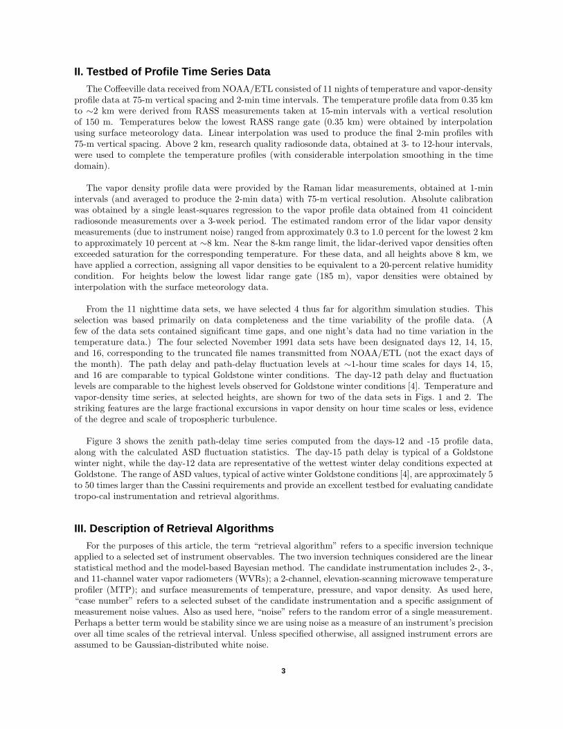
The Coffeeville data received from NOAA/ETL consisted of 11 nights of temperature and vapor-densityprofile data at 75-m vertical spacing and 2-min time intervals. The temperature profile data from 0.35 kmto ∼2 km were derived from RASS measurements taken at 15-min intervals with a vertical resolutionof 150 m. Temperatures below the lowest RASS range gate (0.35 km) were obtained by interpolationusing surface meteorology data. Linear interpolation was used to produce the final 2-min profiles with75-m vertical spacing. Above 2 km, research quality radiosonde data, obtained at 3- to 12-hour intervals,were used to complete the temperature profiles (with considerable interpolation smoothing in the timedomain).
The vapor density profile data were provided by the Raman lidar measurements, obtained at 1-minintervals (and averaged to produce the 2-min data) with 75-m vertical resolution. Absolute calibrationwas obtained by a single least-squares regression to the vapor profile data obtained from 41 coincidentradiosonde measurements over a 3-week period. The estimated random error of the lidar vapor densitymeasurements (due to instrument noise) ranged from approximately 0.3 to 1.0 percent for the lowest 2 kmto approximately 10 percent at ∼8 km. Near the 8-km range limit, the lidar-derived vapor densities oftenexceeded saturation for the corresponding temperature. For these data, and all heights above 8 km, wehave applied a correction, assigning all vapor densities to be equivalent to a 20-percent relative humiditycondition. For heights below the lowest lidar range gate (185 m), vapor densities were obtained byinterpolation with the surface meteorology data.
From the 11 nighttime data sets, we have selected 4 thus far for algorithm simulation studies. Thisselection was based primarily on data completeness and the time variability of the profile data. (Afew of the data sets contained significant time gaps, and one night’s data had no time variation in thetemperature data.) The four selected November 1991 data sets have been designated days 12, 14, 15,and 16, corresponding to the truncated file names transmitted from NOAA/ETL (not the exact days ofthe month). The path delay and path-delay fluctuation levels at ∼1-hour time scales for days 14, 15,and 16 are comparable to typical Goldstone winter conditions. The day-12 path delay and fluctuationlevels are comparable to the highest levels observed for Goldstone winter conditions [4]. Temperature andvapor-density time series, at selected heights, are shown for two of the data sets in Figs. 1 and 2. Thestriking features are the large fractional excursions in vapor density on hour time scales or less, evidenceof the degree and scale of tropospheric turbulence.
Figure 3 shows the zenith path-delay time series computed from the days-12 and -15 profile data,along with the calculated ASD fluctuation statistics. The day-15 path delay is typical of a Goldstonewinter night, while the day-12 data are representative of the wettest winter delay conditions expected atGoldstone. The range of ASD values, typical of active winter Goldstone conditions [4], are approximately 5to 50 times larger than the Cassini requirements and provide an excellent testbed for evaluating candidatetropo-cal instrumentation and retrieval algorithms.
III. Description of Retrieval Algorithms
For the purposes of this article, the term “retrieval algorithm” refers to a specific inversion techniqueapplied to a selected set of instrument observables. The two inversion techniques considered are the linearstatistical method and the model-based Bayesian method. The candidate instrumentation includes 2-, 3-,and 11-channel water vapor radiometers (WVRs); a 2-channel, elevation-scanning microwave temperatureprofiler (MTP); and surface measurements of temperature, pressure, and vapor density. As used here,“case number” refers to a selected subset of the candidate instrumentation and a specific assignment ofmeasurement noise values. Also as used here, “noise” refers to the random error of a single measurement.Perhaps a better term would be stability since we are using noise as a measure of an instrument’s precisionover all time scales of the retrieval interval. Unless specified otherwise, all assigned instrument errors areassumed to be Gaussian-distributed white noise.
3

0 2 4 6 8 10 12 14
UT, h
0.0
0.5
1.0
1.5
2.0
2.5
3.0
3.5
4.0
VA
PO
R D
EN
SIT
Y,
g/m
3
–8
–6
–4
–2
0
2
4
6
8
T (z = 4.01)
V (z = 4.01)
T (z = 2.06 km)
V (z = 2.06)
V (z = 3.03)T (z = 3.03)
TEM
PE
RA
TUR
E, deg C
(b)
Fig. 1. Time series of temperature and vapor density from the lidar and RASS data obtained for day 12 at Coffeeville at heights (a) <2 km and (b) >2 km.
2
3
4
5
6
7
8
9
10
VA
PO
R D
EN
SIT
Y, g
/m3
5
6
7
8
9
10
11
12
13
TEM
PE
RA
TUR
E, deg C
T (z = 0 km)
V (z = 0.41)T (z = 0.41)
V (z = 0)
V (z = 1.46)
T (z = 1.46)
(a)
A. Statistical Algorithms
All statistical algorithms were generated using a 3-year (1990–1992) radiosonde archive from Topeka,Kansas. Topeka is located ∼160 miles due north of Coffeeville and has nearly the same elevation (340 mat Topeka; 290 m at Coffeeville) and similar humidity conditions. The statistical algorithms assume thatthe desired parameter (in our case, zenith wet path delay) can be expressed as a linear combination ofthe instrument observables:
PD = PDmean + Σ Ci(OBi −OBMEANi) (2)
4

0
1
2
3
4
5
6
VA
PO
R D
EN
SIT
Y, g
/m3
–2
0
2
4
6
8
10
12
14
TEM
PE
RA
TUR
E, deg C
T (z = 0 km)
V (z = 0.41)
T (z = 0.41)
V (z = 0)
V (z = 1.46)
T (z = 1.46)
(a)
0 2 4 6 8 10 12
UT, h
0.0
0.5
1.0
1.5
2.0
2.5
3.0
3.5
VA
PO
R D
EN
SIT
Y, g
/m3
–8
–6
–4
–2
0
2
4
6
8
TEM
PE
RA
TUR
E, deg C
T ( z= 4.01)
V (z = 4.01)
T (z = 2.06 km)V (z = 2.06)
V (z = 3.03)
T (z = 3.03)
Fig. 2. Time series of temperature and vapor density from the lidar and RASS data obtained for day 15 at Coffeeville at heights (a) <2 km and (b) >2 km.
(b)
where PDmean is the archive average path delay, OBi is the measured value of the ith observable (com-puted from the profile data), OBMEANi is the computed archive average for the ith observable, and theCi are the linear retrieval coefficients generated by regression of the path delay versus observables-plus-noise archive computed from the radiosonde database. The generated retrieval coefficients depend on theassigned observable noise values because the error vector is added to the observables before regressingwith path delay. Thus, for low-noise cases, the coefficients approach values that would be produced bya simple multilinear regression of computed path delays versus computed observables, and the predictedretrieval error approaches the fit’s rms residual. For high-noise cases, the coefficients approach zero asthe observable information content diminishes, retrieved path delay values remain close to the archiveaverage, and the predicted retrieval error approaches the archive standard deviation in path delay.
5

0 2 4 6 8 10 12 14UT, h
5
6
7
8
9
10
11
12
PD
ZEN
, cm
DAY 12
DAY 15
PDMEAN =ASD (120 s) =
ASD (960 s) = ASD (4800 s) =
DAY 12 DAY 15 9.66 6.54 cm40.5 56.6 x 10⁻¹⁵ s/s10.2 8.0 8.4 2.4
Fig. 3. Zenith wet path delay time series computed from the lidar and RASS measurements at Coffeeville for the day-12 and day-15 intervals.
B. Bayesian Algorithms
The Bayesian method employs model-based inversion techniques to solve the radiative transfer equationfor discrete vapor and temperature profiles given the array of observable measurements. The profiles arevaried iteratively, with theoretical observables calculated each step, until a most-probable profile solutionis obtained. From this most-probable profile solution, the final retrieved path delay is computed directly.The criteria for a most-probable solution include constraints based on a priori covariance statistics of theprofiles as well as the residuals between measured and computed observables. The covariance statisticsare derived from the same Topeka radiosonde archive used for the statistical algorithms and provide ameans for downweighting a profile solution that varies too greatly from the archive mean. In qualitativeterms, the most-probable profile solution is that which minimizes the residuals between measured andcomputed observables while best conforming to the constraints of the a priori statistics.
Observable errors are taken into account by adjusting the relative weights assigned to the residual andstatistical constraints. Similarly to the statistical algorithms, higher observable errors lead to increasedweight for the a priori archive and less weight for the measurements.
IV. Retrieval Simulation Procedures
For each of the four selected lidar-plus-RASS nighttime profile data sets, 2-min time series of pathdelay and all candidate observables were computed by numerical solution of the radiative transfer equationusing our current nominal model of atmospheric absorption and refractivity. All candidate observablesused in the first two stages of testing are listed in Table 1 along with the range of associated Gaussianerrors that have been considered.
The range of WVR brightness temperature errors spans worst-to-best cases in the sense that poorlymonitored gain variations can easily result in 0.5-K drifts over multihour periods, while 0.01 K repre-sents the multihour stability goal of the advanced WVR. Current WVRs, with careful gain drift mon-itoring, have demonstrated stability at the 0.1-K level. The stability of current generation ground-based MTPs is less certain, but the 0.1- to 1.0-K range probably brackets the actual performance. The
6

Table 1. Candidate observables and associated errors.
Observable no. Description Frequency, GHz Elevation angle, deg Error range, K
1 WVR TBa 20.0 90 0.01–0.50
2 WVR TB 20.4 90 0.01–0.50
3 WVR TB 20.7 90 0.01–0.50
4 WVR TB 21.2 90 0.01–0.50
5 WVR TB 21.7 90 0.01–0.50
6 WVR TB 22.235 90 0.01–0.50
7 WVR TB 22.7 90 0.01–0.50
8 WVR TB 23.2 90 0.01–0.50
9 WVR TB 23.6 90 0.01–0.50
10 WVR TB 24.0 90 0.01–0.50
11 WVR TB 31.4 90 0.01–0.50
12 MTP TB 54.4 90 0.10–1.00
13 MTP TB 54.4 42 0.10–1.00
14 MTP TB 54.4 30 0.10–1.00
15 MTP TB 57.97 90 0.10–1.00
16 MTP TB 57.97 42 0.10–1.00
17 MTP TB 57.97 30 0.10–1.00
18 Surface temperature — — 0.2 K
19 Surface pressure — — 1.0 mb
20 Surface vapor density — — 0.5 g/m3
a TB = brightness temperature.
single-point estimates of surface meteorology observable precision are values that are commonly cited andthat we assume are attainable with carefully calibrated off-the-shelf technology.
Using the computed “truth” time series of observables as algorithm inputs, retrieval simulations wereperformed for individual cases by selecting an observable subset, adding Gaussian noise of the specifiedlevel to each 2-minute observable array, and then retrieving the time series of zenith path delay over the10- to 12-hour interval of the selected lidar-based data set. The time series of retrieval error (retrieved-minus-truth path delay) was then computed, and measures of performance, including bias, scatter, anderror ASD, were calculated. Evaluations were then made comparing algorithm techniques (Bayesianversus statistical) and different observable subsets, and assessing the effects of measurement stability.When comparing the retrieval-error ASD results with the Cassini requirements and goals, it is importantto note that the first-stage retrieval simulations were performed for zenith path delay only, an overlyoptimistic comparison in that the retrieval errors will scale with air mass and the actual Cassini trackingwill be very nearly sidereal. This issue is addressed in Section VI.
V. First-Stage Results
The initial selection of test cases was intended to provide insights on the following main issues:
(1) When, if at all, are Bayesian techniques clearly superior to statistical ones for path delayretrieval?
7

(2) What improvements can be obtained by adding channels to the standard three-frequencyWVR?
(3) How much improvement is afforded by adding MTP and surface meteorology observables?
In the first stage of simulations, 24 cases were selected to investigate the above issues. These cases arelisted in Table 2 in terms of observable selection and assigned errors.
Table 2. First-stage simulation case description.
Error
Case no. Observable
WVR, K MTP, K Ts, K Ps, mb Vs, g/m3
1 3-channel WVR 0.50 — — — —
2 3-channel WVR 0.10 — — — —
3 3-channel WVR 0.03 — — — —
4 3-channel WVR 0.01 — — — —
5 11-channel WVR 0.50 — — — —
6 11-channel WVR 0.10 — — — —
7 11-channel WVR 0.03 — — — —
8 11-channel WVR 0.01 — — — —
9 3-channel WVR +Ts 0.01 — 0.2 — —
10 3-channel WVR +Ps 0.01 — — 1.0 —
11 3-channel WVR +Vs 0.01 — — — 0.5
12 3-channel WVR +Ts + Ps + Vs 0.01 — 0.2 1.0 0.5
13 11-channel WVR +Ts 0.01 — 0.2 — —
14 11-channel WVR +Ps 0.01 — — 1.0 —
15 11-channel WVR +Vs 0.01 — — — 0.5
16 11-channel WVR +Ts + Ps + Vs 0.01 — 0.2 1.0 0.5
17 3-channel WVR +MTP + Ts 0.01 1.0 0.2 — —
18 3-channel WVR +MTP + Ts 0.01 0.5 0.2 — —
19 3-channel WVR +MTP + Ts 0.01 0.1 0.2 — —
20 3-channel WVR +MTP + Ts + Ps + Vs 0.01 0.1 0.2 1.0 0.5
21 11-channel WVR + MTP +Ts 0.01 1.0 0.2 — —
22 11-channel WVR + MTP +Ts 0.01 0.5 0.2 — —
23 11-channel WVR + MTP +Ts 0.01 0.1 0.2 — —
24 11-channel WVR + MTP +Ts + Ps + Vs 0.01 0.1 0.2 1.0 0.5
Note that “3-channel WVR” refers to the standard JPL WVR J-unit operating frequencies of 20.7, 22.2,and 31.4 GHz, while “11-channel WVR” refers to the full ensemble of WVR frequencies listed in Table 1.For all cases that include MTP measurements, a two-channel (54.4- and 57.97-GHz) elevation-scanningsystem is simulated with sky brightness temperature measurements at 30-, 42-, and 90-deg elevations. Inan earlier unpublished study, this frequency and elevation combination has been determined to be nearoptimum for temperature profile retrievals for heights up to 5 to 7 km.
Retrievals for observable set case numbers 1 through 24 were simulated for the testbed data setsdesignated days 12, 14, 15, and 16 using both the Bayesian and statistical methods. Results are shownin Figs. 4 through 7 in terms of retrieval error bias and ASD. The most significant result in terms of bias
8

(Fig. 4) is that Bayesian methods applied to advanced WVR-plus-MTP observable sets (cases 17 through24) always reduce the retrieved path delay bias to a level of ∼0.01 cm or less, even for MTP errors aslarge as 1.0 K. For cases without MTP observables (1 through 16), the biases have little or no correlationwith WVR errors. This result suggests that the nonlinear model-based algorithms, when temperatureprofiling observables are included, effectively eliminate offsets due to pervasive conditions that departfrom the statistical archive average.
–0.20
–0.15
–0.10
–0.05
0.00
0.05
0.10
0.15
0.20
PD
RE
TRIE
VA
L B
IAS
, cm
BAYESIANSTATISTICAL
3-CH WVR
11-CH WVR
3-CH WVR+ SURF MET
11-CH WVR + SURF MET
3-CH WVR+ MTP + Ts
11-CH WVR + MTP + Ts
3-CH WVR
11-CH WVR
3-CH WVR+ SURF MET
11-CH WVR + SURF MET
3-CH WVR+ MTP + Ts
11-CH WVR + MTP + Ts
(a) (b)
–0.20
–0.15
–0.10
–0.05
0.00
0.05
0.10
0.15
0.20
PD
RE
TRIE
VA
L B
IAS
, cm
(c) (d)
0 5 10 15 20 25
CASE NUMBER
3-CH WVR
11-CH WVR
3-CH WVR+ SURF MET
11-CH WVR + SURF MET
3-CH WVR+ MTP + Ts
11-CH WVR + MTP + Ts
0 5 10 15 20 25
3-CH WVR
11-CH WVR
3-CH WVR+ SURF MET
11-CH WVR + SURF MET
3-CH WVR+ MTP + Ts
11-CH WVR + MTP + Ts
CASE NUMBER
Fig. 4. A comparison of Bayesian and statistical path delay retrievals in terms of bias for the Coffeeville testbed data. The case numbers refer to specific selections of observables and observable errors (see Table 2 and the text for a more detailed description): (a) day 12, (b) day 14, (c) day 15, and (d) day 16.
Figures 5 through 7 show the retrieval error ASD for three time scales that nearly span the GWEintervals of interest. Also indicated on the plots are the Cassini ASD requirements (CR) and goals (CG)1
and annotated information describing the observables and observable errors for each case number. (Forfurther clarification, refer to Table 2.) Note that the Cassini specifications shown in Figs. 5 through 7have been scaled downward by a 1/
√2 factor to account for the two-way tracking required by Cassini.
(For two-way tracking, the ASD of the retrieval error increases by a factor of approximately√
2, assumingthe uplink and downlink retrieval errors are uncorrelated. This will be the case as long as the Cassinisignal round-trip travel time is greater than the ASD time scale of interest.)
1 Cassini Radio Science Ground System D-Level and Cost Review (internal document), Jet Propulsion Laboratory,Pasadena, California, February 27, 1995.
9

102030405060708090100
ASD x 1015, s/s
CR
CG
3-C
H W
VR
0.1 0.
03
0.01
0.1
0.03
0.01
3-C
H W
VR
+
11-C
H W
VR
+
11-C
H W
VR
T sP
sV
s
T s Ps
Vs
3-C
H W
VR
+M
TP +
Ts
+
1.0
0.5
0.1
0.11.
00.
5
0.1
0.1
σ WV
R =
0.0
1
T s
Ps
Vs
T s Ps
Vs
σ MTP
=P
sV
s
Ps
Vs
AS
D (P
Dtru
) = 4
0.5
BA
YE
SIA
NS
TATI
STI
CA
L
σ WV
R =
0.5
0.5
11-C
H W
VR
+M
TP +
Ts
+
(a)
1.0
0.5
0.1
0.11.
00.
5
0.1
0.1
(b)
AS
D (P
Dtru
) = 4
6.8
CR
CG
05
1015
2025
CA
SE
NU
MB
ER
1.0
0.5
0.1
0.1
1.0
0.5
0.1
0.1
(c)
0
CR
CG
102030405060708090100
ASD x 1015, s/s
00
510
1520
25
CA
SE
NU
MB
ER
1.0
0.5
0.1
0.1
1.0
0.5
0.1
0.1
(d)
CR
CG
Fig
. 5.
A
co
mp
aris
on
of
Bay
esia
n a
nd
sta
tist
ical
pat
h d
elay
ret
riev
als
in t
erm
s o
f A
SD
at
a 12
0-s
tim
e in
terv
al f
or
the
Co
ffee
ville
tes
tbed
dat
a.
Th
e ca
se
nu
mb
ers
refe
r to
sp
ecif
ic s
elec
tio
ns
of
ob
serv
able
s an
d o
bse
rvab
le e
rro
rs (
see
Tab
le 2
an
d t
he
text
fo
r a
mo
re d
etai
led
des
crip
tio
n):
(a)
day
12,
(b
) d
ay 1
4,
(c)
day
15,
an
d (
d)
day
16.
3-C
H W
VR
11-C
H W
VR
σ WV
R =
0.0
1
3-C
H W
VR
+3-
CH
WV
R +
MT
P +
Ts
+σ M
TP =
11-C
H W
VR
+M
TP
+ T
s +
0.1 0.
030.
01
0.1 0.
03
0.01
0.5
σ WV
R =
0.5
T sP
sV
s
T s Ps
Vs
11-C
H W
VR
+
T sP
s
Vs
T s Ps
Vs
Ps
Vs
Ps
Vs
AS
D (P
Dtru
) = 3
5.4
σ WV
R =
0.0
1
3-C
H W
VR
σ WV
R =
0.5
0.1 0.
03
0.01
11-C
H W
VR
0.
5
0.1 0.
03
0.01
3-C
H W
VR
+ T s Ps
Vs
T s
Ps
Vs
11-C
H W
VR
+ T s Ps
Vs
T sP
sV
sσ M
TP =
3-C
H W
VR
+M
TP
+ T
s + Ps
Vs
11-C
H W
VR
+M
TP
+ T
s + Ps
Vs
σ WV
R =
0.5
3-C
H W
VR
0.1 0.
03
0.01
0.1 0.
03
0.01
11-C
H W
VR
0.5
σ WV
R =
0.0
1
AS
D (P
Dtru
) = 5
8.6
3-C
H W
VR
+11
-CH
WV
R +
3-C
H W
VR
+M
TP +
Ts
+
11-C
H W
VR
+M
TP +
Ts
+
T s
Ps
Vs
T s Ps
Vs
T s Ps
Vs
T sP
sV
sσ M
TP =
Ps
Vs
Ps
Vs
10

ASD x 1015, s/s
CR
CG
3-C
H W
VR
0.1
0.03
0.01
0.
1
0.03
0.01
3-C
H W
VR
+
11-C
H W
VR
+
11-C
H W
VR
T sP
sV
s
T s Ps
Vs
3-C
H W
VR
+M
TP +
Ts
+
1.0
0.5
0.1
0.1
1.0
0.5
0.1
0.1
σ WV
R =
0.0
1
T s
Ps
Vs
T s Ps
Vs
σ MTP
=P
sV
s
Ps
Vs
AS
D (P
Dtru
) = 1
0.2
BA
YE
SIA
NS
TATI
STI
CA
Lσ W
VR
= 0
.5
0.5
11-C
H W
VR
+M
TP +
Ts
+
(a)
1.0
0.5
0.1
0.1
1.0
0.5
0.1
0.1
(b)
AS
D (P
Dtru
) = 6
.9
CR
CG
05
1015
2025
CA
SE
NU
MB
ER
1.0
0.5
0.1
0.1
1.0
0.5
0.1
0.1
(c)
CR
CG
ASD x 1015, s/s
0
510
1520
25
CA
SE
NU
MB
ER
1.0
0.5
0.1
0.1
1.0
0.5
0.1
0.1
(d)
CR
CG
Fig
. 6.
A
co
mp
aris
on
of
Bay
esia
n a
nd
sta
tist
ical
pat
h d
elay
ret
riev
als
in t
erm
s o
f A
SD
at
a 96
0-s
tim
e in
terv
al f
or
the
Co
ffee
ville
tes
tbed
dat
a.
Th
e ca
se
nu
mb
ers
refe
r to
sp
ecif
ic s
elec
tio
ns
of
ob
serv
able
s an
d o
bse
rvab
le e
rro
rs (
see
Tab
le 2
an
d t
he
text
fo
r a
mo
re d
etai
led
des
crip
tio
n):
(a)
day
12,
(b
) d
ay 1
4,
(c)
day
15,
an
d (
d)
day
16.
3-C
H W
VR
11-C
H W
VR
σ WV
R =
0.0
1
3-C
H W
VR
+3-
CH
WV
R +
MT
P +
Ts
+σ M
TP =
11-C
H W
VR
+M
TP
+ T
s +
0.1 0.
030.
01
0.1 0.
03
0.01
0.5
σ WV
R =
0.5
T sP
sV
s
T s Ps
Vs
11-C
H W
VR
+
T sP
s
Vs
T s Ps
Vs
Ps
Vs
Ps
Vs
AS
D (P
Dtru
) = 5
.4
σ WV
R =
0.0
1
3-C
H W
VR
σ WV
R =
0.5
0.1 0.
03
0.01
11-C
H W
VR
0.
5
0.1
0.03
0.01
3-C
H W
VR
+ T s Ps
Vs
T s
Ps
Vs
11-C
H W
VR
+ T s Ps
Vs
T sP
sV
sσ M
TP =
3-C
H W
VR
+M
TP
+ T
s + Ps
Vs
11-C
H W
VR
+M
TP
+ T
s + Ps
Vs
σ WV
R =
0.5
3-C
H W
VR
0.1 0.
03
0.01
0.1
0.03
0.01
11-C
H W
VR
0.5
σ WV
R =
0.0
1
AS
D (P
Dtru
) = 8
.0
3-C
H W
VR
+
11-C
H W
VR
+3-
CH
WV
R +
MTP
+ T
s +
11-C
H W
VR
+M
TP +
Ts
+
T s
Ps
Vs
Ts Ps
Vs
T s Ps
Vs
T sP
sV
sσ M
TP =
Ps
Vs
Ps
Vs
024681012
024681012
11

ASD x 1015, s/s
CR
CG
3-C
H W
VR
0.1 0.
03
0.01
0.
1
0.03
0.01
3-C
H W
VR
+
11-C
H W
VR
+
11-C
H W
VR
T s
Ps
Vs
T s Ps
Vs
3-C
H W
VR
+M
TP +
Ts
+
1.0
0.5
0.1
0.1
1.0
0.5
0.1
0.1
σ WV
R =
0.0
1
T s
Ps
Vs
Ts Ps
Vs
σ MTP
=P
sV
s
Ps
Vs
AS
D (P
Dtru
) = 8
.4
BA
YE
SIA
NS
TATI
STI
CA
Lσ W
VR
= 0
.5
0.5
11-C
H W
VR
+M
TP +
Ts
+
(a)
1.0
0.5
0.1
0.1
1.0
0.5
0.1
0.1
(b)
AS
D (P
Dtru
) = 2
.8
CR
CG
05
1015
2025
CA
SE
NU
MB
ER
1.0
0.5
0.1
0.1
1.0
0.5
0.1
0.1
(c)
CR
CG
ASD x 1015, s/s
05
1015
2025
CA
SE
NU
MB
ER
1.0
0.5
0.1
0.1
1.0
0.5
0.1
0.1
(d)
CR
CG
Fig
. 7.
A
co
mp
aris
on
of
Bay
esia
n a
nd
sta
tist
ical
pat
h d
elay
ret
riev
als
in t
erm
s o
f A
SD
at
a 48
00-s
tim
e in
terv
al f
or
the
Co
ffee
ville
tes
tbed
dat
a.
Th
e ca
se
nu
mb
ers
refe
r to
sp
ecif
ic s
elec
tio
ns
of
ob
serv
able
s an
d o
bse
rvab
le e
rro
rs (
see
Tab
le 2
an
d t
he
text
fo
r a
mo
re d
etai
led
des
crip
tio
n):
(a)
day
12,
(b
) d
ay 1
4,
(c)
day
15,
an
d (
d)
day
16.
3-C
H W
VR
11-C
H W
VR
σ WV
R =
0.0
1
3-C
H W
VR
+
3-C
H W
VR
+M
TP
+ T
s +
σ MTP
=
11-C
H W
VR
+M
TP
+ T
s +
0.1 0.
03 0.01
0.1
0.03
0.01
0.5
σ WV
R =
0.5
T s
Ps
Vs
Ts Ps
Vs
11-C
H W
VR
+
T sP
sV
s
T s Ps
Vs
Ps
Vs
Ps
Vs
AS
D (P
Dtru
) = 1
.5
σ WV
R =
0.0
1
3-C
H W
VR
σ WV
R =
0.5
0.1 0.
03
0.01
11-C
H W
VR
0.
5
0.1 0.
03
0.01
3-C
H W
VR
+ T s Ps
Vs
T s
Ps
Vs
11-C
H W
VR
+ T s Ps
Vs
T sP
sV
sσ M
TP =
3-C
H W
VR
+M
TP
+ T
s + Ps
Vs
11-C
H W
VR
+M
TP
+ T
s + Ps
Vs
σ WV
R =
0.5
3-C
H W
VR
0.1 0.
03
0.01
0.1
0.03
0.01
11-C
H W
VR
0.5
σ WV
R =
0.0
1
AS
D (P
Dtru
) = 2
.4
3-C
H W
VR
+
11-C
H W
VR
+3-
CH
WV
R +
MTP
+ T
s +
11-C
H W
VR
+M
TP +
Ts
+
T s
Ps
Vs
Ts Ps
Vs
T s Ps
Vs
T sP
sV
sσ M
TP =
Ps
Vs
Ps
Vs
0.0
0.5
2.5
2.0
1.5
1.0
0.0
0.5
2.5
2.0
1.5
1.0
12

Based on the results shown in Figs. 5 through 7, and addressing the three issues outlined above, wedraw the following conclusions:
(1) In terms of ASD, Bayesian retrievals are clearly superior to statistical methods whentemperature profile information (MTP) is available (cases 17 through 24). At the shortertime scales (∆t = 120 s, Fig. 5), the Cassini requirements can only be approached byutilizing Bayesian techniques with precise WVR and MTP observables. At the longertime scales (Figs. 6 and 7), the Cassini goals can be met or exceeded using the Bayesiantechniques with the precise WVR-plus-MTP observable set. When only WVR or WVR-plus-surface meteorology observables are available (cases 1 through 16), the results aremixed. For the testbed data sets of days 14, 15, and 16, the Bayesian results are generallyas good or better than the statistical. For day 12, the statistical retrievals are superiorfor non-MTP cases.
(2) The addition of channels in the 20- to 24-GHz band to the standard three-channel WVRproduces no significant retrieval improvement in the ASD domain, with or without MTPand surface meteorology observables, when the WVR errors are less than 0.1 K. In fact,for WVR precision approaching the goal of the advanced WVR (0.01 to 0.03 K), theASD performance is actually significantly worse for the 11-channel system relative tothe standard 3-channel WVR when no MTP observables are used. (Compare cases 5through 8 with 1 through 4 and cases 13 through 16 with 9 through 12.) This behavioroccurs for both the Bayesian and statistical retrievals at all time scales, and we haveno definitive explanation for it at this time. One contributing factor appears to be theeffect of increasing system noise with the addition of WVR channels. Theoretically, thisshould not occur. If the covariance matrices are correctly calculated, the addition of re-dundant or low information observables should not increase the retrieval noise. However,examination of the statistical algorithms’ retrieval coefficients reveals the opposite to beoccurring. From Eq. (2), it is straightforward to derive the retrieval noise that resultsfrom independent observable noise:
∆PD =[Σ(Ci[∆OBi])2
]1/2(3)
where ∆PD is the retrieval noise and ∆OBi are the observable errors. Because theobservable errors are considered random, the ∆PD values are easily converted into ASDvalues using Eq. (1). The result is that the system noise is the dominant component ofthe statistical algorithm ASD values shown in Figs. 5 through 7 and is responsible for thedegradation in performance going from the 3-channel to the 11-channel WVR observablesets. This result suggests that, for low WVR observable noise (<0.1 K) and stronglyinformation-redundant observables, the correlations of observables with path delay arenot being accurately calculated, due either to the inadequacy of the Topeka data archivefor resolving small differences in the effects of path delay on observables or errors thatare amplified in the inversion of a near-singular regression matrix.
We have also investigated the performance of a two-channel WVR for the Cassini tropo-cal system to evaluate trade-offs between performance and the design simplification andcost reductions afforded by a two-channel (versus three-channel) radiometer. The is-sue was addressed using WVR-plus-MTP-plus-Ts observable sets including two-channel(20.7-, 31.4-GHz and 22.2-, 31.4-GHz) and three-channel (20.7-, 22.2-, and 31.4-GHz)WVRs with wide ranges of WVR and MTP errors. The simulations were performedusing only the Bayesian algorithm on testbed days 12 and 15, which had the largest andmost variable path delay. The results indicated that for all tested combinations of WVRand MTP errors the three-channel WVR system produces better ASD performance. The
13

fractional improvement generally increases as both the WVR and MTP errors decrease.For the low range of errors considered (<0.03 K for the WVR and <0.3 K for the MTP),the three-channel reduction in the retrieval error ASD (relative to the best two-channelresult) ranges approximately from 20 to 50 percent for the three time scales of 120, 960,and 4800 seconds. Based on these results, we concluded that a three-channel WVR isthe optimum choice for the Cassini tropo-cal system.
(3) With advanced WVR precision (0.01 K) and a Bayesian algorithm, the addition ofMTP (and the surface temperature) observables produces dramatic improvement in theASD domain of retrieval performance (cases 17 through 24). The performance dependsstrongly on the MTP observable errors, improving by a factor of approximately 2 to 4times as the MTP errors are reduced from 1.0 to 0.1 K. For the best-case MTP observ-ables, with 0.1-K precision (cases 19, 20, 23, and 24), Cassini requirements for near-zenithtracking are met or exceeded at all time scales. These results appear to be insensitive tothe variation in fluctuation levels seen in the four testbed data sets.
The addition of surface pressure and surface vapor density as observables does not ap-pear to significantly improve performance (e.g., compare cases 19 and 20). However,considering the relatively low cost of deployment and other uses, such as monitoringof the dry delay component and calibration checks on the microwave instrumentation,a surface meteorology package, including temperature, pressure, and humidity sensors,should be included in the Cassini tropo-cal system design.
VI. Second-Stage Results
Analysis of retrieval simulations for the initial 24 candidate sets of observables and observable errorsled to three main conclusions: (1) The advanced WVR for Cassini tropo-cal needs no additional channelsbeyond the standard three-channel WVR system; (2) inclusion of an MTP or equivalent temperature pro-filing system is required to attain optimal tropospheric calibration; and (3) Bayesian retrieval techniquesare required to maximize performance for a tropo-cal system that includes advanced WVR precision andMTP observables.
In the second stage of simulations, three remaining issues were addressed using the lidar testbed dataset: (1) optimization of the three-frequency WVR channel selection, (2) the effects of sidereal line-of-sighttracking, and (3) the effects of WVR calibration offsets.
A. Optimization of the Three-Frequency WVR Channel Selection
We have assumed to this point that the frequencies of the three-channel WVR include the vaporresonance line center (22.235 GHz), the lower-frequency “hinge” point (20.7 GHz, see below), and acloud-sensitive channel (31.4 GHz) identical to the J-series WVRs designed at JPL. From previous studies(e.g., [2]), these frequencies have been determined to be near-optimum for WVR-only path-delay retrievalaccuracy in both clear and cloudy weather. For the Cassini GWE, which requires unprecedented precisionin tropospheric calibration, and is expected to primarily utilize cloud-free data, the 31.4-GHz channelmay not be optimum, and we decided to investigate possible improvements afforded by replacing the31.4-GHz channel with a lower frequency near the vapor line.
To address the frequency selection issue, we ran simulations for numerous three-frequency combinationswith the following results. Line center (22.235 GHz) and a frequency within ∼0.5 GHz of the absorptionline hinge points are required to achieve optimal retrieval performance. The line center provides maximumsignal-to-noise ratio in terms of water vapor sensitivity. The hinge points, near 20.7 and 23.8 GHz, are leastsensitive to the height distribution of the vapor due to pressure broadening effects. There is considerablelatitude, however, in the choice of the third frequency for clear conditions. This is shown in Fig. 8. The
14

DAY 12
DAY 14
DAY 15
DAY 16
22 23 24 25 26 27 28 29 30 31 32
THIRD FREQUENCY, GHz
0.2
0.3
0.4
0.5
0.6
0.7
0.8
0.9
1.0
1.1
1.2
RE
TRIE
VA
L E
RR
OR
AS
D (x
10–
15),
s/s
CASSINI REQUIREMENT (a)
23.3 23.4 23.5 23.6 23.7 23.8 23.9 24.0 24.1 24.2
CASSINI REQUIREMENT
0.2
0.3
0.4
0.5
0.6
0.7
0.8
0.9
1.0
1.1
1.2
RE
TRIE
VA
L E
RR
OR
AS
D (x
10–
15),
s/s
(b)
THIRD FREQUENCY, GHz
Fig. 8. The dependence of the retrieval error ASD at a 960-s time scale on the choice of a third WVR frequency for the 4 days of Coffeeville testbed data, where the first two frequencies are (a) 20.7 and 22.235 GHz and (b) 22.235 and 31.4 GHz.
upper panel displays the retrieval error ASD (at a 960-s time scale) versus the choice of the third WVRfrequency for the four nights of lidar testbed simulations. For this case, line center and the 20.7-GHzhinge point have been chosen as the primary vapor-sensing channels. Note that there is no significantperformance impact for selected third frequencies in the range of 25 to 31.4 GHz and that performanceactually deteriorates if the third frequency is chosen closer to the 22.235-GHz vapor line center. Theseresults also indicate that there is no significant advantage in clear weather of replacing the 31.4-GHzchannel with a lower frequency. Thus, based on the expectation that the Cassini GWE will desire a“best-effort” performance during cloudy conditions, it is recommended that the 31.4-GHz channel beretained as the third frequency in the advanced WVR design.
The lower panel of Fig. 8 shows the sensitivity of ASD performance as the hinge frequency is variedover a 0.8-GHz range surrounding 23.8 GHz. Here we have assumed the line center and the 31.4-GHzcloud-sensing channel as the two given frequencies. The essentially flat result indicates that the hinge
15

point frequency can be varied by at least ±0.4 GHz without significantly degrading the ASD retrievalperformance. Results are very similar at the 120- and 4800-s time scales and suggest that we will have suf-ficient flexibility in frequency selection to avoid potential problems, such as radio frequency interference(RFI), that could restrict our channel options. Assuming no restrictions, our WVR frequency recom-mendation would be 22.235, 23.8, and 31.4 GHz. (The 23.8-GHz hinge point yields slightly better ASDperformance than the 20.7-GHz channel.) We will hereafter refer to this WVR frequency combination,coupled with the MTP and surface meteorology observables, as the nominal Cassini GWE troposphericcalibration system.
B. The Effects of Sidereal Line-of-Sight Tracking
Path delay and path-delay fluctuation levels increase with air mass. All simulations to this pointhave assumed constant zenith observations, for which the line-of-sight delay errors are minimized. Forsidereal tracking of Cassini, line-of-sight calibration will be required for all spacecraft positions above20-deg elevation, and the question remains of how the retrieval errors will scale with air mass. It isnot necessary to simulate the continuous elevation variation of sidereal tracking to address this issue.Because the effective speed of sidereal tracking through the troposphere is much less than the wind speed,the retrieval error ASD results will not differ significantly from the case of fixed-elevation observationsobtained at the midpoint elevation of any Cassini tracking interval. To investigate the worst-case scenario,we have repeated the lidar testbed simulations using the nominal GWE calibration system, but with theWVR pointing fixed at 20-deg elevation, the maximum air mass encountered during Cassini tracking.The result of the fixed 20-deg simulation is that the ASD of the line-of-sight retrieval error increasesby a factor of three relative to the fixed zenith case, the same factor as the air mass ratio between20-deg elevation and zenith. Thus, we have confirmed in the ASD domain that the retrieval error willscale linearly with air mass, and the tropospheric calibration system performance relative to Cassinirequirements must be evaluated accordingly. The results shown in Figs. 5 through 7 are representative ofnear-zenith tracking. For elevation angles above 60 deg, corrections to the predicted ASD performanceshown in Figs. 5 through 7 will be less than 15 percent. At the lowest tracking elevations (20 to 40 deg),the predicted retrieval error ASD values will increase by a factor of from 1.5 to 3.0 relative to the resultsshown in Figs. 5 through 7. The implications for meeting the Cassini GWE requirements at all timescales and elevation angles are discussed further in Section VII.
C. The Effects of WVR Calibration Offsets
The radiometer instrument errors to this point have been assumed to be purely stochastic with zerobias. The question remains of the effect of realistic instrument calibration offsets, in particular offsetsthat vary with WVR channel. To evaluate the effects of offsets, we have repeated the retrieval simulationsfor days 12 and 15, using the nominal calibration system (22.235-, 23.8-, and 31.4-GHz WVR plus MTPplus surface meteorology), but with 1-K offsets added to one, two, or all three WVR channel observables.For all cases, significant path-delay retrieval biases (0.1 to 0.5 cm) occurred. As expected, the case forwhich all three channel biases were set to 1 K produced no significant degradation in ASD performance;i.e., the retrieval error did not vary significantly with time. However, for cases in which only one or two ofthe WVR channels contained 1-K offsets, ASD performance degraded by approximately 40 to 60 percent,dependent both on the testbed data set (day 12 or 15) and on which of the channels included the offset.Thus, relative WVR channel offsets can be expected to degrade the tropo-cal performance, and effortsshould be made to ensure that the actual relative offsets are limited to a level less than ∼0.5 K.
We also simulated relative offsets in the MTP measurements and found the effects to be much less thanthose for comparable WVR offsets. The worst case examined assumed a +1 K offset for the 54.4-GHzchannel and a −1 K offset for the 57.97-GHz channel, producing an approximate 10-percent degradationin ASD performance over the 960- and 4800-second time scales. MTP offset effects at the 120-secondtime scale were insignificant for all cases considered in which relative channel offsets did not exceed 2 K.
16

VII. Nominal System Performance Versus Radiometer Stability
Thus far the retrieval simulations have been used to establish a prototype tropospheric calibrationsystem consisting of a three-channel (22.235-, 23.8-, and 31.4-GHz) WVR, a two-channel (54.4- and 57.97-GHz) MTP, and a three-component surface meteorology package. If the targeted radiometer stabilitygoals (0.01 K for the advanced WVR and 0.1 K for the MTP) are met, the nominal tropo-cal systemwill meet or exceed the GWE requirements at all time scales for the near-zenith (approximately >60-degelevation) portion of Cassini sidereal tracking. To assess the degradation of performance in the event thatthe radiometric stability goals cannot be met, we have repeated the simulations using the nominal tropo-cal system for wide ranges of assumed WVR and MTP stability that span the targeted and worst-caseperformance range. The simulations were performed on the day-12 and day-15 testbed profiles, assuminga constant line-of-sight elevation angle of 45 deg, an intermediate value for Cassini tracking intended tobe representative of mean air mass conditions for the GWE. The results for day 12 are shown in Fig. 9 ascontour plots of two-way retrieval error ASD versus WVR and MTP stability. Results for day 15 differedfrom day 12 by less than 20 percent at all time scales. The values designated “CR” and “CG” in theplots are the Cassini requirements and Cassini goals, respectively, for two-way tropospheric calibration.Note that the contours represent the net effect of the retrieval algorithm plus instrument stability errorcomponents.
From the results shown in Fig. 9, we draw the following conclusions regarding the impact of radiometerstability on the performance of the prototype Cassini tropo-cal system:
(1) At the 120-s time scale [Fig. 9(a)], the estimated ASD performance for targeted radiome-ter stability (0.01 and 0.1 K for the WVR and MTP) is approximately 8 × 10⁻¹⁵ s/s,approximately 30-percent higher than the Cassini requirement. Any significant degrada-tion in radiometer stability would lead rapidly to unacceptable performance. However,at this short time scale, it is expected that the stated radiometer stability goals will bemost easily achieved, and very possibly surpassed, producing tropospheric calibrationperformance very close to the GWE requirements.
(2) For intermediate time scales [960 s, Fig. 9(b)], the Cassini requirement is matched withradiometer errors approximately 2 to 3 times as large as the best case considered (0.01 Kfor the WVR and 0.1 K for the MTP). We note that, while the stated design goal for theadvanced WVR is 0.01-K stability, no comparable analysis has yet been made of MTPstability limitations. Our WVR experience suggests that 0.1-K MTP stability should beattainable, but further analysis is needed of the existing ground-based MTP instruments.
(3) For the largest time scales relevant to the GWE [>4000 s, Fig. 9(c)], the retrieval-plus-stability error component should make no significant contribution to the Cassini ASDrequirement. In fact, if we are within a factor of three in meeting the radiometer stabilitytargets, the GWE goal at ∆t > 1-hour time scales would be comfortably met for nearlyall segments of the Cassini sidereal track.
VIII. Conclusions and Future Work
Simulations of path delay retrieval over approximate 10-hour intervals, using real data for the timevariation of atmospheric conditions, indicate that a tropo-cal system consisting of a three-channel WVR,two-channel MTP, and surface meteorology measurements is required to meet the Cassini GWE spec-ifications. A model-based Bayesian inversion algorithm is also required to minimize retrieval errors inthe ASD domain. Recommended channels for the advanced WVR are 22.2, 23.8, and 31.4 GHz, withthe additional note that any frequency in the range from 23.4 to 24.2 GHz could replace the 23.8-GHzchannel with no significant performance impact.
17

0.0
0.1
0.2
0.3
0.4
0.5
0.6
0.7
0.8
0.9
1.0
MTP
STA
BIL
ITY
, K
2-WAY ASD = 12 x 10–15 s/s
16
20
24
28
32CR = 6.0 x 10⁻¹⁵ CG = 1.5 x 10⁻¹⁵
2-WAY ASD = 1.6 x 10⁻¹⁵ s/s
2.4
3.2
4.0
4.8
CR = 1.6 x 10⁻¹⁵ CG = 0.4 x 10⁻¹⁵
0.0
0.1
0.2
0.3
0.4
0.5
0.6
0.7
0.8
0.9
1.0
MTP
STA
BIL
ITY
, K
0 0.01 0.02 0.03 0.04 0.05 0.06 0.07 0.08 0.09 0.10
WVR STABILITY, K
2-WAY ASD = 0.3 x 10⁻¹⁵ s/s
0.4
0.5
0.6
0.7CR = 1.6 x 10⁻¹⁵ CG = 0.4 x 10⁻¹⁵
0.8
0.0
0.1
0.2
0.3
0.4
0.5
0.6
0.7
0.8
0.9
1.0
MTP
STA
BIL
ITY
, K
Fig. 9. Contour plots of the ASD of the two-way retrieval error at a 45-deg elevation versus WVR and MTP instrument stability for the day-12 testbed data at a dt of (a) 120 s, (b) 960 s, and (c) 4800 s.
(a)
(b)
(c)
18

If the targeted radiometer stability goals (0.01 K for the WVR and 0.1 K for the MTP) are achieved,the simulations indicate that the proposed tropospheric calibration system will meet or surpass the CassiniGWE requirements at almost all relevant time scales and elevation angles. At the shortest time scale(∼100 s), the retrieval algorithm error component alone will approximately match the GWE requirement,with only slight improvement afforded by improvements in radiometer stability. At the intermediate(∼1000-s) time scale, the targeted radiometer stabilities can be relaxed by a factor of approximatelythree and still meet the Cassini requirements. For hour time scales and longer, the retrieval algorithmplus radiometer stability error components will not be significant relative to the GWE requirements. Atthe ∼5000-s time scale, the specified Cassini goal (0.4 × 10⁻¹⁵ s/s ASD) could be met with WVR andMTP stabilities of 0.03 and 0.3 K, respectively.
The stated tropospheric calibration system performance would be significantly degraded by rela-tive WVR channel offsets of ∼1-K magnitude. For example, simulations performed with a +1-K off-set in the 23.8-GHz WVR channel, and a zero offset in all other radiometer channels, produced a60-percent degradation in the day-12 ASD performance and a 40-percent degradation in the day-15performance. Offsets common to all three WVR channels produced no significant degradation in ASDperformance. Similar analyses of the effects of MTP offsets showed much smaller effects, with an approx-imate 10-percent ASD performance degradation in the extreme case of a 2-K relative offset between thetwo MTP channels.
Recent laboratory measurements of the advanced WVR prototype stability conducted by Dr. AlanTanner of JPL’s Microwave, Lidar, and Interferometer Technology Section suggest that the 0.01-K goalcould be surpassed at <1-hour time scales. At a 1000-s time scale, 0.005-K performance is typical. Atshorter time scales, the stability becomes thermal noise limited, with a precision level of ∼0.003 K for a100-s integration time. Dr. Tanner also estimates that planned calibration tests for the advanced WVRwill constrain channel calibration relative offsets to the 0.1- to 0.2-K level. An important near-future testfor the advanced WVR will be to determine if the stability goals can be achieved outside the controlledlaboratory environment.
The stability of current generation MTPs over 10-hour time scales needs to be assessed to determineif precision levels approaching 0.1 K are attainable. Alternative temperature profiling instrumentation(such as RASS) should also be considered, evaluating trade-offs between cost, reliability, and stability.The assumed precision of surface meteorology instrumentation should also be investigated. Of particularimportance is determining the availability of temperature and pressure sensors with precision at the 0.2-Kand 1-mb level, respectively.
Acknowledgments
The authors thank R. Linfield and M. J. Mahoney for their very useful commentsin reviews of preliminary drafts of this article.
References
[1] D. W. Allan, “Statistics of Atomic Frequency Standards,” Proc. IEEE, vol. 54,no. 2, pp. 221–230, 1966.
19

[2] B. L. Gary, S. J. Keihm, and M. A. Janssen, “Optimum Strategies and Perfor-mance for the Remote Sensing of Path Delay Using Ground-Based MicrowaveRadiometers,” IEEE Trans. Geosci. Rem. Sensing, vol. GE-23, pp. 479–484,1985.
[3] Y. Han, J. B. Snider, E. R. Westwater, S. H. Melfi, and R. A. Ferrare, “Obser-vations of Water Vapor by Ground-Based Microwave Radiometers and RamanLidar,” JGR, vol. 99, pp. 18,695–18,702, 1994.
[4] S. J. Keihm, “Water Vapor Radiometer Measurements of the Tropospheric DelayFluctuations at Goldstone Over a Full Year,” The Telecommunications and DataAcquisition Progress Report 42-122, April–June 1995, Jet Propulsion Laboratory,Pasadena, California, pp. 1–11, August 15, 1995.http://tda.jpl.nasa.gov/tda/progress report/42-122/122J.pdf
20