I

ADVANCED 3D RENDERING: ADAPTIVE CAUSTIC MAPS USING COMPUTE SHADER

A Major Qualifying Project Report:

Submitted to the Faculty

of the

WORCESTER POLYTECHNIC

INSTITUTE

In partial fulfillment of the requirements for

the Degree of Bachelor of Science

By

Yong Piao

Date: April 30nd, 2015

Approved:

______________________________

Professor Emmanuel Agu, Major Advisor

II

Table of Contents

Abstract ........................................................................................................................................ III

Acknowledgements ...................................................................................................................... IV

List of Figures ............................................................................................................................... V

Introduction ................................................................................................................................... 1

Background ................................................................................................................................... 5

Methodology ............................................................................................................................... 22

Implementation ........................................................................................................................... 26

Results and Discussions .............................................................................................................. 33

Conclusions and Recommendations ............................................................................................ 42

References ................................................................................................................................... 43

Appendix ..................................................................................................................................... 45

III

Abstract

Graphics researchers have long studied real-time caustic rendering. The state-of-the-

art technique Adaptive Caustic Maps provides a novel way to avoid densely sampling

photons during a rasterization pass, and instead adaptively emits photons using a deferred

shading pass. In this project, we present a variation of adaptive caustic maps for real-

time rendering of caustics. Our algorithm is conceptually similar to Adaptive Caustic

Maps but has a different implementation based on the general-purpose computing

pipeline provided by OpenGL version 4.3. Our approach accelerates the photon splitting

process using compute shaders and bypasses various other performance overheads,

ultimately speeding up photon generation considerably.

IV

Acknowledgements

I would like to thank Professor Emmanuel Agu and Che Sun for their advice and support.

Both their enthusiasm and insight on this subject were crucial to the completion of this work.

V

List of Figures

Figure 1: Example of caustics formed by refractive objects ................................................. 2

Figure 2: Photograph of an underwater scene ..................................................................... 3

Figure 3: The caustic mapping process ................................................................................ 6

Figure 4: Photon buffer at resolution of 162 with many unused photons.............................. 9

Figure 5: Normal textures of the dragon model rendered from the side ............................ 10

Figure 6: Result of rendering the dragon from the side ...................................................... 11

Figure 7: Normal textures of the dragon model rendered from the back ........................... 11

Figure 8: Result of rendering the dragon from the back .................................................... 12

Figure 9: Workflow of Adaptive Caustic Maps ................................................................... 13

Figure 10: OpenGL rendering stages with transform feedback ......................................... 15

Figure 11: Compute shader work groups ........................................................................... 19

Figure 12: Workflow of our approach with compute shaders ............................................ 23

Figure 13: Traversing a 42 kernel with 4 work groups ....................................................... 24

Figure 14: Structure of the indirect command buffer ......................................................... 26

Figure 15: Sampling kernel initialization ........................................................................... 27

Figure 16: Photon buffer layout .......................................................................................... 27

Figure 17: The initialization shader ................................................................................... 28

Figure 18: Declaring an atomic counter in GLSL .............................................................. 29

Figure 19: Writing new photons to the photon buffer ......................................................... 30

Figure 20: Code snippet of post-traversal statistics shader ............................................... 30

Figure 21: Update read and write parameters in the statistics shader .............................. 31

Figure 22: Update draw count in the statistics shader ....................................................... 31

Figure 23: Structure of indirect draw command buffer ...................................................... 31

Figure 24: Render result with a 40962 photon buffer. ........................................................ 34

Figure 25: Caustic map rendered at 642 ............................................................................. 35

Figure 26: Caustic map rendered at 1282 ........................................................................... 35

Figure 27: Caustic map rendered at 2562 ........................................................................... 36

Figure 28: Caustic map rendered at 5122 ........................................................................... 36

Figure 29: Caustic map rendered at 10242 ......................................................................... 37

Figure 30: Caustic map rendered at 20482 ......................................................................... 37

Figure 31: Caustic Map rendered at 40962 ........................................................................ 38

Figure 32: Chart of best case scenario frame rate vs. work group size ............................. 39

Figure 33: Chart of worst case scenario framerate vs. work group size ............................ 40

1

Introduction

Video games have become increasingly popular. “The industry is at around $22

billion for 2008 (conservative estimate) in the US1 and $30 to $40 billion globally,”

while “The movie industry is at $9.5 billion (US)2 and $27 billion globally3.” Due to the

inter-disciplinary nature of video game development, video games have also brought

benefits to the concept art, 3d modeling, and music industries.

Computer graphics plays a key role in the presentation of video games. It is the sole

source of stimuli to the players’ visual perception. As a result, many game developers

continuously seek to improve the visual realism in their games. Due to the interactive

nature of video games, graphics must be presented at an interactive frame rate (25 FPS

minimum). Therefore rendering speed is highly valued for any rendering technique in

the field of real-time computer graphics.

Burdened with its firm requirement of high rendering speed and the limited

processing speed of current rendering hardware, real-time rendering forces graphics

researchers to seek rendering techniques that provide both high image quality and fast

1 Frank Caron, June 18 2008. Ars Technica. http://arstechnica.com/news.ars/post/20080618-gaming-expected-to-be-

a-68-billion-business-by-2012.html 2 Thomas Mennecke, March 6, 2007. Slyck.

http://www.slyck.com/story1436_MPAA_Reports_Record_Movie_Sales_in_2006 3 Reuters, March 5 2008. ABC News. http://www.abc.net.au/news/stories/2008/03/06/2181568.htm

2

rendering speed. Nonetheless, real-time rendering is steadily heading towards

photorealism with interactivity. For example, with Enlighten4, a Global Illumination (GI)

plug-in developed by Geomerics, it is now possible to simulate highly realistic first-

bounce reflective light in real-time. Enlighten can make dynamic lights look highly

realistic, however, as an example of commercial GI solution, Enlighten is limited to

computing GI for diffuse transport 5 . The rendering of curved refractive, reflective

surfaces with global illumination remains unsolved.

One key component of rendering curved refractive, reflective surfaces is caustics.

In Optics, a caustic or caustic network is the envelope of light rays reflected or refracted

by a curved surface or object6. Figure. 1 shows 4 glass spheres rendered with various

refraction indices. Clearly caustics contributes a lot to differentiating refractive and

opaque objects, as well as improving the realism of the rendering.

Figure 1: Example of caustics formed by refractive objects

4 Geomeric, an ARM company, 2014. http://www.geomerics.com/enlighten/ 5 Jesper Mortensen. September 18, 2014. Technology in Unity 5, http://blogs.unity3d.com/2014/09/18/global-

illumination-in-unity-5/ 6 Lynch DK and Livingston W, 2001. Color and Light in Nature. Cambridge University Press. ISBN 978-0-521-

77504-5. Chapter 3.16 The caustic network, Google books preview

3

Figure. 2 is a photograph of an underwater scene; again clearly shows caustics is

essential for the rendering of photorealistic computer images.

Figure 2: Photograph of an underwater scene

Many existing techniques provide rendering of caustics in real-time. There are

techniques that use "image-space approximations [OB07, Wym05], object-space

approximations [EMDT06, RH06], and ray-based [KBW06, SZS*08] approaches to

allow applications to quickly simulate simple reflections and refractions, though fully

accurate renderings generally remain too costly.”

Adaptive caustic maps [Wym09], provides a novel technique for adaptively

sampling photons, allowing dynamic quality control for applications and at the same

time improving rendering speed. It uses a hierarchical sampling method to avoid

processing extraneous photons, thus greatly reduces the amount of unnecessary

computation required when compared to basic caustic maps at the same image quality.

Though much faster than before, adaptive caustic maps remains too costly for video

games.

4

The Goal of this Major Qualifying Project (MQP)In this project, we

present a variation of adaptive caustic maps for real-time rendering of caustics. Our

algorithm is conceptually similar to adaptive caustic maps: traversing through a buffer

of sample points, splitting them into more photons, and finally splatting photons onto a

caustics texture. However, by using the general-purpose computing pipeline provided by

OpenGL version 4.3, our approach uses compute shaders to perform the traversal process,

and drawing indirectly using indirect command buffer to avoid CPU-side overheads.

The goal of this project is to use graphics hardware to solve the “poor parallelism

during early traversal steps, and high memory consumption for photon storage” [Wym09]

and to reduce the CPU-side overhead of Adaptive Caustic Maps. At the end our approach

achieved great parallelism through compute shaders and removed CPU-side overhead

completely.

5

Background

Graphics researchers have long studied Global Illumination algorithms. “The earliest

path tracing techniques [Kaj86] demonstrated caustics from reflective and refractive

objects.” Unfortunately, computational costs prohibit real time use of path tracing for

interactive media and games, and most fast global illumination algorithms restrict scenes

to diffuse materials.

A number of researchers have already come up with advanced techniques to allow

interactive rasterization of non-diffuse materials. For the purpose of this project, basic

Caustic Mapping and Adaptive Caustic Maps will be illustrated to help provide a

comparison to our project. For both techniques, when rendering caustics, scene geometry

generally is separated into two categories, receiver geometry and refractor geometry. The

receiver geometry receives the computed photon texture, e.g. floors, walls, and other

background objects. The refractor geometry refract the photons that hit the geometry to

create photon density map, e.g. glass spheres, metallic rings.

Basic Caustic Mapping

Below is the most basic, 3-step Caustic Mapping, taken from Caustics Mapping: An

Image-Space Technique for Real-Time Caustics by Musawir et al. [Mus07]:

1. Obtain position texture of the receiver geometry from light’s point of view.

6

2. Obtain position and front and back normal textures of the refractor geometry from

light’s point of view.

3. Construct caustic map texture based on the three textures obtained above.

Figure 3: The caustic mapping process

Figure 3 illustrates the procedure of caustic mapping. There are always 2 refractions

per light ray, because when light ray hits the refractive object, it is conceptually the same

as entering the object. Every ray that enters a refractive object must also exit the refractive

object to be captured by the receiver object. Therefore when rendering caustics with high

fidelity, both front and back normal textures are needed for the correct calculation of

refraction.

Musawir et al. also provide detailed explanation of the mathematics behind caustic

mapping. Let v be the direction of the light ray, we can then access the light-view front

7

normal texture to obtain the normal vector n. After refraction, the light ray r is produced.

The direction of point P from the light is thus:

Equation 1: Point of intersection of refracted ray [Mus07]

Although it is possible to render refractor position textures to find the root of the

intersection, the depth values from normal textures can be utilized for obtaining a much

finer result. This method is also inherently fast because depth textures can be added to the

normal textures and handled by OpenGL:

Equation 2: Calculating front and back face intersection with depth values

In order to calculate the final exiting ray, one more refraction is needed. We repeat

the process of calculating P, but instead use the new ray r as the incident ray direction

and n’ as the new normal vector to obtain r’. The back face refraction in the Caustic

Mapping algorithm uses an iterative method derived from the Newton-Raphson algorithm

for calculating the intersection with the receiver object, thus the distance d’ can be derived

as follows: [Mus07]

Equation 3: The Newton-Raphson algorithm [Mus07]

Equation 3 shows the Newton-Raphson algorithm for iteratively calculating the

8

distance between two surfaces. We can thus obtain P’ through plugging in r’, and d’ to

Equation 1.

Musawir et al. pointed out that “frustum limitation and aliasing” [Mus07] are the 2

main problems with this technique. Specifically the first issue pertaining to the algorithm

is the view frustum limitation during rasterization of the caustic-map. Musawir et al.

mentioned that this problem is “exactly like that of shadow mapping with point lights.”

[Mus07] If the caustics are formed outside the light’s view frustum, they will not be

captured on the caustic-map texture. Using an environment caustic map solves this

problem at an overhead cost of rendering extra textures. However, Musawir et al.

suggested that the dual paraboloid mapping technique proposed by Heidrich [Hei98],

which has been applied to shadow mapping for omnidirectional light sources by Brabec

et al. [Bra02], can also be utilized.

The second issue with Caustic Mapping is aliasing. Since “aliasing is inherent in all

image-space algorithms,” [Mus07], “the gaps between the point splats give a non-

continuous appearance to the caustics.” [Mus07] However, according to the author, “if

there is a sufficient number of vertices in the refractive vertex grid, the gaps are

significantly reduced.” [Mus07]

Though unmentioned by Musawir et al., we found Caustic Mapping inherently

9

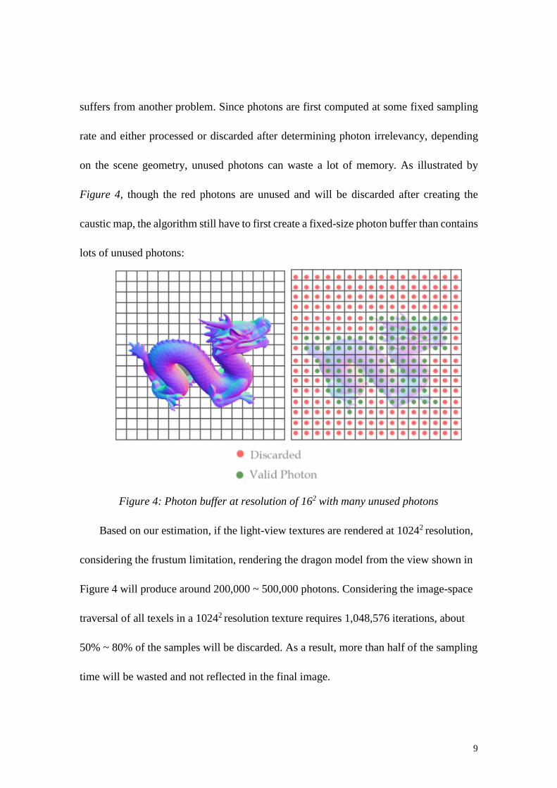
suffers from another problem. Since photons are first computed at some fixed sampling

rate and either processed or discarded after determining photon irrelevancy, depending

on the scene geometry, unused photons can waste a lot of memory. As illustrated by

Figure 4, though the red photons are unused and will be discarded after creating the

caustic map, the algorithm still have to first create a fixed-size photon buffer than contains

lots of unused photons:

Figure 4: Photon buffer at resolution of 162 with many unused photons

Based on our estimation, if the light-view textures are rendered at 10242 resolution,

considering the frustum limitation, rendering the dragon model from the view shown in

Figure 4 will produce around 200,000 ~ 500,000 photons. Considering the image-space

traversal of all texels in a 10242 resolution texture requires 1,048,576 iterations, about

50% ~ 80% of the samples will be discarded. As a result, more than half of the sampling

time will be wasted and not reflected in the final image.

10

Temporal incoherency is another problem that we found with Caustic Mapping in

interactive applications. The conclusion was that because Caustic Mapping only uses 2

layers of normal textures, the initial sample obtained from rendering the refractor

geometry is crucial to the image quality. We noticed that fidelity of the image decreases

if there are many overlapping faces. When the dragon model is rendered from its side, we

can obtain normal textures similar to Figure 5:

Figure 5: Normal textures of the dragon model rendered from the side

The side view camera helps minimizing the number of overlapping faces in the normal

textures, therefore it helps converge the rendered result to ground truth. As shown in

Figure 5, the result texture contains noticeable amount of caustics:

11

Figure 6: Result of rendering the dragon from the side

On the other hand, certain camera views can increase the number of overlapping faces,

and reduce the surface area of valid normal texels. Figure 7 shows the dragon rendered

from the back. In this case, the normal textures contain many overlapping faces that

cannot be accurately captured by 2 normal textures. This would not only impact the

photon traversal process, but also reduce the number of samples to start with.

Figure 7: Normal textures of the dragon model rendered from the back

Figure 8 shows the result from using normal textures rendered from the back. Clearly the

12

head and neck part of the normal textures cannot not provide the number of samples

required to generate enough valid photons for a satisfying caustic texture.

Figure 8: Result of rendering the dragon from the back

Adaptive Caustic Maps

The state-of-the-art Adaptive Caustic Maps [Wym09] overcomes the aliasing

problem and the fix-sized photon buffer problem of Caustic Mapping through “emitting

a few photons, and adaptively refining with additional photons until the desired quality is

attained.” [Wym09] Algorithmically, since Wyman el al. propose to adaptively splitting

photons, “instead of first creating a photon buffer and then processing it to generate a

caustic map, these two steps become coupled.” [Wym09] Adaptive Caustic Maps “never

creates an explicit photon buffer. Instead, an adaptive deferred shading pass that point-

samples the geometry buffers allows us to emit photons adaptively.” [Wym09]

13

Figure 9: Workflow of Adaptive Caustic Maps

There is only one step in generating photons with Adaptive Caustic Maps. However

it is up to the application how many times it would like to run the same step to increase

the number of photons in the photon buffer. Figure 9 illustrates the basic workflow of

executing the photon splitting of Adaptive Caustic Maps three times with a 42 kernel to

start with. Since only the valid photons from the previous pass will be used to split

photons in a later iteration, the amount of unused photons generated is much less than

basic Caustic Mapping. Also because Adaptive Caustic Maps does not process all normal

texels in one shader pass, it requires the refractor normal textures to have hardware

accelerated mip-maps enabled. The mip-map enabled refractor normal textures are used

14

so the normal texels can be traversed as a quadtree, allowing the algorithm to greatly

reduce extraneous photons.

As a result, Adaptive caustic maps reduces the overhead from processing extraneous

photons and also allows applications to dynamically control of the level of detail for

caustic map, ultimately making basic Caustic Mapping obsolete. While this technique

made caustic mapping practical in real-time, it is still not fast enough for interactive media

and games.

Problems with Adaptive Caustic Maps

There are three main points of concern with Adaptive Caustic Maps that this project

addresses. Wyman et al. mentioned the first two in the paper: 1) “poor parallelism during

early traversal steps, and 2) high memory consumption for photon storage provided

challenges”[Wym09]. In addition, we also found an extant CPU-side overhead that was

inevitable when Adaptive Caustic Maps was published.

Adaptive Caustic Maps makes heavy use of OpenGL “with the transform feedback

and geometry shader extensions.”[Wym09] Wyman et al. mentioned that “characteristics

of the GPU stream processing model affected numerous design choices for Adaptive

Caustic Maps as well as performance.”[Wym09]. Clearly the GPU stream processing

model with transform feedback suffers from poor parallelism and is imperfect for photon

15

generation, which results in an impact on the performance of the algorithm.

Figure 10: OpenGL rendering stages with transform feedback

Figure 10 illustrates the rendering stages of OpenGL with transform feedback

enabled. Transform feedback is “the process of capturing Primitives generated by the

Vertex Processing step(s), recording data from those primitives into Buffer Objects.”7

Transform feedback allows an application to “preserve the post-transform rendering state

of an object and resubmit this data multiple times.”8 It made the use of vertex and

geometry shader more flexible, allowing vertex and geometry shader to output data

without a-priori knowledge of the output buffer size.

Since the number of output photons for Adaptive Caustic Maps is determined during

7 The Khronos Group, 2010-2014. OpenGL Wiki. https://www.opengl.org/wiki/Transform_Feedback 8 The Khronos Group, 2010-2014. OpenGL Wiki. https://www.opengl.org/wiki/Transform_Feedback

16

rendering, transform feedback comes in play where after executing the geometry shading

stage, it gives the application a message containing the number of primitives generated

during transform feedback. With this information, the application can perform a new

photon traversal iteration with the output from the last iteration.

Due to the implementation of the GPU stream processing model of OpenGL,

transform feedback requires that the application always binds input and output buffers to

different buffer targets. As shown in Figure 9, Adaptive Caustic Maps must flip-flop

between 2 buffers during photon splitting. This not only introduces increasingly heavy

CPU-side overheads, but also requires two large buffers that are big enough to contain all

information generated from the last iteration. Before each new iteration, the application

must bind input and output buffers to new buffer targets, therefore the more iterations of

traversal the application decides to perform, the heavier the CPU-side overhead becomes.

Poor parallelism also occurs because when sampling a photon, Adaptive Caustic

Maps must use the vertex shader to pass a point primitive to the geometry shader.

OpenGL strictly requires that a vertex shader can only process one vertex at a time,

making loop unroll impossible to perform.

In addition, Adaptive Caustic Maps requires the application to pass in new drawing

arguments and setting appropriate uniforms for sampling, which also becomes an

17

increasingly expensive CPU-side overhead as the number of iteration increases.

Our approach is conceptually similar to Adaptive Caustic Maps; in fact the math

involved is nearly identical. We also use hardware accelerated mip-maps on normal

textures and perform quad-tree traversal to reduce extraneous photons as Adaptive

Caustic Maps. However, instead of using the geometry shader and transform feedback,

we use the new general-purpose processing pipeline of OpenGL to perform the most

expensive photon traversal process instead of using geometry shader with transform

feedback. Our approach solves two main problems of Adaptive Caustic Maps with great

parallelism and zero CPU-side overhead.

Compute Shader

In order to understand the new traversal process, it is crucial to have a basic

understanding of the compute shader. In 2012, OpenGL 4.3 introduced arbitrary compute

shaders. It is revolutionary to performing general-purpose computation on the GPU,

allowing highly optimized, parallel tasking for caustic photon traversal. It allows

applications to smoothly pass the data from general-purpose computing pipeline to the

drawing pipeline, ultimately benefiting any real-time rendering algorithm that can make

use of general-purpose computation. In the case of caustic mapping, photon splitting is a

perfect example of a general-purpose computation task that can become highly parallel

through the use of compute shader.

18

Compute shaders operate differently from other shader stages and is completely

separate from the drawing pipeline. While all of the other shaders have a well-defined set

of input and output values, though some build-in and some user-defined, compute shader

does not. When an application executes a compute shader, it provides the compute shader

with a set of parameters specifying the number of invocations to execute the program.

In its most basic form, if a very simple compute shader, such as one that increments

a variable atomically by 1, is asked by the application to execute with 240 invocations,

the variable will be incremented by 240. However a real compute shader is slightly

different. A real compute shader has the concept of a work group (a grouping of GPU

threads); and an application can specify the number of work groups to execute.

While the number of work groups that a compute shader is executed is defined by the

application, the work groups are actually organized in three dimensional space. Therefore

the application must provide the X, Y, and Z values specifying the “compute space” for

the compute shader. An example would be splitting 240 into X=24, Y=10, and Z = 1. As

a result, an application can specify the number work groups of a compute space, a

compute shader can define the number of “workers” in a work group. In addition, every

compute shader has a three-dimensional local size, again customizable via X, Y, and Z

values, specifying the number of invocations triggered by a work group. As a result, the

19

total invocation count must take into account the number of work groups and the size of

work groups.

Figure 11: Compute shader work groups9

Figure. 11 illustrates an example of a compute space specification. There are 4 by 5, a

total of 20 work groups. In addition, the compute shader defines that each work group

has a size of 4 by 3 by 1, a total of 12 invocations. Therefore each time this compute

task is dispatched, the program will be run a total of 240 times.

Since the application can freely control how many times a compute shader is

executed, it should be simple to imagine how to traverse through a 642 sampling kernel.

One may choose to distribute the 642 sampling invocations by any appropriate work

9The Khronos Group, 2010-2014. http://www.slideshare.net/Khronos_Group/how-to-use-and-teach-opengl-compute-shaders

20

group specification, for the purpose of this project, we chose to keep the Z size at 1 for

ease of visualization.

One potential problem with working with compute shaders is the compute space

might end up dispatching more invocations than needed. If the application needs to

iterate through a total of 17 elements in a buffer, there is no value of integer X such that

X2 = 17, because 17 is a prime number. The least possible resolution for a texture that

contains more than 17 pixels is 52 = 25. Since the application only requires 17

computations, the extra 8 invocations must return immediately and not change any data.

One way to accomplish this is to use the OpenGL compute shader built-in inputs to

calculate the global invocation ID prior to performing a task, thereby giving the 25

invocations IDs from 0 to 24 respectively. With a globally unique ID for each

invocation, to achieve a total of 17 invocations, the compute shader can set any

invocation with an ID equal to or higher than 17 to immediately return.

Indirect Dispatch

Before stepping into the implementation, it is also crucial to know about the indirect

compute dispatch feature. As described above, the application can specify the size of the

compute workspace, which means the CPU must calculate the number of work groups

needed and send this data to the GPU. However during its calculation and data transfer,

the GPU stands completely idle, as a result making this time period a CPU-side overhead.

21

To combat this issue, OpenGL provides a feature to let the GPU autonomously dispatch

a compute task, in which case the application need not to specify the number of work

groups to execute. To use this feature, the application must bind a buffer containing 3

unsigned integers to the indirect command buffer target. Once the buffer is created, it is

up to the shaders to decide how to change the data in the buffer, therefore making it

possible to autonomously use the GPU to determine the workspace size for a compute

shader.

Indirect Draw

Similar to indirect dispatch, the indirect draw feature allows the GPU to

autonomously draw without passing arguments from the CPU. Our approach uses indirect

draw to further reduce the CPU-size overhead. To use this feature, the application must

bind a buffer containing 4 unsigned integers to the indirect command buffer target. Once

the buffer is created, the GPU can dynamically change the vertex count to correspond to

the current drawing settings.

22

Methodology

In summary, our approach uses compute shaders and indirect draw to replace

geometry shader and transform feedback used by Adaptive Caustic Maps. We reckon that

the repetitive task of computing millions of photons through Adaptive Caustic Maps

renders the OpenGL drawing pipeline unfit. The iterative photon splitting of the original

Adaptive Caustic Maps, on the other hand, is a perfect example of a general-purpose

computation task that can be accelerated with compute shaders. In addition, with compute

shaders, it is possible to read and write from the same buffer using atomic operations,

avoiding flip-flopping between buffers. In the end, our approach solves two main

problems of Adaptive Caustic Maps with great parallelism and zero CPU-side overhead.

23

Figure 12: Workflow of our approach with compute shaders

Figure 12 illustrates the workflow of our approach. As opposed to the original Adaptive

Caustic Maps, our approach uses only one photon buffer. It is made possible because

with proper synchronization, compute shaders can read and write to the same buffer. As

a result, our approach does not have flip-flopping between input and output buffers like

the original implementation, thus removes the CPU-side overhead from re-binding

buffers completely.

We also use the compute shader work groups to achieve parallelism during photon

24

traversal. Since a compute shader dispatch can specify the number of work groups and

the size of a work group, it inherently allows the shader to perform loop unroll on the

repetitive sampling operation.

Figure 13: Traversing a 42 kernel with 4 work groups

Figure 13 illustrates traversing a 42 photon buffer with 4 work groups. Instead of

dispatching 16 work groups, we can choose to increase the size of the work group to

obtain high parallelism. It is important to notices that with the work group size being

2x2x1, the number of work groups to dispatch is 2x2 instead of 4x4. In the end, we

found parallelism through compute shader work groups provides a major performance

increase. We also provide performance analysis on different work group sizes in the

results section.

Synchronization of invocations in the compute shader is conceptually similar to

25

multi-threaded programming. OpenGL provides an atomic counter feature that can be

used to coordinate between different invocations. Upon validation of a photon, the

invocation handling that photon will increment the atomic counter, so that no other

invocation will use the old atomic counter value for calculating the write index.

26

Implementation

With a basic understanding of the compute shader and indirect dispatch, it is possible

to go through the caustic map generation process.

Pre-Traversal Initialization

First, the application must create a structure containing 3 unsigned integers that can be

used as an indirect command buffer, as shown in Figure 14:

Figure 14: Structure of the indirect command buffer

Then, the application must create a sampling kernel on initialization. Figure 15 shows an

example of creating a two-dimensional sampling kernel with the x and y values

representing the u and v coordinates for texture sampling:

27

Figure 15: Sampling kernel initialization

After generating the sampling kernel, we immediately copy the data to a photon buffer as

if these sampling points are actual photons. The photon buffer is a 1-demensional array

used to store sampling points that will be used in the splatting process, as shown in Figure

16:

Figure 16: Photon buffer layout

The actual photon traversal process is broken up into 3 stages, each representing a

complete compute shader program: initialization, traversal, and post-traversal statistics.

The initialization shader is run once per frame; its sole purpose is to initialize data

buffers such as the indirect command buffer and various other parameters required for

photon traversal completely on the GPU to minimize CPU-size overhead. For example,

if the application decides to deploy a 642 sampling kernel, the initialization shader can set

the primitive count to 4096, and use this number to set the values in the indirect command

buffer to X=64, Y=64, Z=1, so that the traversal shader can be dispatched, again without

sending any uniform data from the CPU to the GPU. Figure. 17 shows a code snippet of

the initialization shader used in the demo program:

28

Figure 17: The initialization shader

Notice the num_groups_x and num_groups_y in the ACMIndirectCommandBuffer are

set to 8 and 8, which seems to not produce the right amount of photons. It is because the

traversal shader uses a work group of size 8 by 8 by 1, therefore ultimately the number of

invocations is 84=4096.

Since our approach uses one photon buffer for all iterations, read and write offsets

are required to into the 1-dimensional photon buffer correctly. In the first traversal, the

read offset is 0 because the traversal shader should read the sampling points defined by

the kernel generated during application initialization. The write offset is 4096 because the

application stores the 642 sampling point grid into a 1-dimensional array, and in order to

29

utilize all sampling points in the kernel, none should ever be over-written. To achieve so

we append new data to the end of the buffer instead of overwriting previous data.

Effectively, a read offset of 0 and read count of 4096 provides traversal shader the input

indices, and a write offset of 4096 tells the shader where to append the new photons.

Without going into much detail, the post-traversal statistics shader is used to update these

parameters to prepare for the next traversal.

Traversal

After initialization, it is now possible to run the traversal shader. Writing the data to the

photon buffer is tricky, because the compute shader is highly parallel, buffer access must

be manually synchronized with the atomic counter. An atomic counter can be declared in

a compute shader, as shown in Figure 18:

Figure 18: Declaring an atomic counter in GLSL

Each time a valid photon is read, the traversal shader increments the write count counter

by 1. Combined with the write offset, the shader can obtain the next available buffer index

for writing photon data. Figure 19 illustrates the process of incrementing the atomic

counter, calculating the new write index, calculating the new sample points and finally

writing the data to the buffer:

30

Figure 19: Writing new photons to the photon buffer

Post-Traversal Statistics

After each traversal, post-traversal statistics shader will update the parameters to the

appropriate values for another traversal. It uses the write count counter from the traversal

shader to update the number of work groups for the indirect command buffer, as shown

in Figure. 20:

Figure 20: Code snippet of post-traversal statistics shader

The statistics shader also needs to update the read and write offset and the read count, as

shown in Figure 21:

31

Figure 21: Update read and write parameters in the statistics shader

Because the statistics shader does not know whether or not the application would like to

perform another iteration of photon traversal, it must also update the indirect command

buffer for splatting the photons, as shown in Figure 22:

Figure 22: Update draw count in the statistics shader

Splatting with Indirect Draw

The application can decide how many iterations of traversal it would like to perform

easily because nearly all data used for photon traversal is self-contained on the GPU.

After a satisfying number of traversals, the application can use the indirect draw

command buffer to splat the photons onto a texture. Figure. 23 illustrates the structure of

indirect draw command buffer used by OpenGL:

Figure 23: Structure of indirect draw command buffer

We can visualize the photons as a point cloud with lots of vertices, so the instance count

is always set to 1. First and base instance are set to 0; they are offset variables unneeded

32

for the purpose of this project.

This concludes the caustics traversal and splat process with compute shader. We

found out that cache optimizations within compute work groups impacts the sampling

speed, and different work group sizes can impact performance significantly, so we tested

various work group sizes and found a work group size of 8 by 8 by 1 to be the most

optimal in our situation. One may find it different depending on her hardware and shader

implementation.

33

Results and Discussions

Results presented below were benchmarked on an 8-core Intel Xeon processor at

3.0GHz with a GeForce GTX 980. Adaptive Caustic Maps using transform feedback:

98,000 photons/ms (40962, 3,300,000 photons / 35FPS)

Our implementation using compute shaders:

410,000 photons/ms (81922, 19,000,000 photons / 25FPS)

Best cases

FPS/Workgroup Size

Iterations resolution 1 x 1 2 x 2 4 x 4 8 x 8 16 x 16

6 64 122 117 123 123 120

7 128 118 113 118 119 118

8 256 113 110 115 116 115

9 512 106 107 112 111 110

10 1024 85 97 102 101 99

11 2048 50 65 72 73 72

12 4096 20 33 36 37 37

Table 1: Best case scenario framerate with different workgroup sizes

Worst cases

FPS/Workgroup Size

Iterations resolution 1 x 1 2 x 2 4 x 4 8 x 8 16 x 16

6 64 113 108 114 113 112

7 128 109 105 110 111 109

8 256 104 102 108 108 107

9 512 96 98 104 102 103

10 1024 73 85 90 88 87

11 2048 35 49 54 54 54

12 4096 11 18 21 22 21

Table 2: Worst case scenario framerate with different workgroup sizes

34

Figure 24: Render result with a 40962 photon buffer.

As shown in Figure 24, our result contains more noise than the original implementation.

It is due to the texture sampling operation on mip-map enabled textures unable to

perform linear interpolation correctly. It is perhaps due to a bug with the graphics driver

of our development hardware. We are still investigating this issue during the writing of

this paper.

35

Figure 25 – Figure 31 presented below illustrate an example of 7 levels of caustic detail

that may be adopted by interactive media and games:

Figure 25: Caustic map rendered at 642

Figure 26: Caustic map rendered at 1282

36

Figure 27: Caustic map rendered at 2562

Figure 28: Caustic map rendered at 5122

37

Figure 29: Caustic map rendered at 10242

Figure 30: Caustic map rendered at 20482

38

Figure 31: Caustic Map rendered at 40962

39

Figure 32 shows the best case scenarios of rendering caustics at different caustic map

resolutions. Best case scenarios are when objects are rendered at such an angle so that it

happens to generate the least amount of valid pixels in the normal textures.

Figure 32: Chart of best case scenario frame rate vs. work group size

40

Worst case scenarios are when objects are rendered at such an angle so that it happens

to generate the most amount of valid pixels in the normal textures.

Figure 33: Chart of worst case scenario framerate vs. work group size

Both Figure 32 and Figure 33 demonstrate great performance increase with parallelism

through compute shaders. We find 8x8x1 to be the most optimal work group size for

caustic maps with 20482 or higher resolutions.

41

Without loss of generality, we think any previously expensive real-time rendering

algorithm that requires massive general-purpose computation can greatly benefit from

using the compute shader. The compute pipeline is highly optimized for parallel

computations and is very flexible because there are no input or output constraints like

the traditional drawing pipeline. No doubt there are still many optimizations that can be

done to push this boundary even further.

42

Conclusions and Recommendations

In this project, we have presented an implementation of the Adaptive Caustics Maps

algorithm that uses compute shaders and indirect draw to eliminate previously occurring

bottlenecks. Though the performance increase turned out to be higher than expected, we

think there is still room for improvement. Perhaps there will be a major performance

increase by optimizing the compute shader instructions and also performing loop unroll

within the compute shader in addition to our utilization of work group based parallelism.

We also think reusing part of the photon buffer that will not be used anymore is a

possible direction for reducing memory consumption for high quality caustic maps. For

example, after 3 photon traversal iterations, photons from the first and second iterations

have expired and can perhaps be managed for reuse. Perhaps one can implement the

compute shader to not only append to the end of the buffer, but also write to expired areas.

43

References

Papers:

[Kaj86] KAJIYA J.: The rendering equation. In Proc. ACM SIGGRAPH (1986), pp.

143–150.

[RH06] ROGER D., HOLZSCHUCH N.: Accurate specular reflections in real-time.

Comput. Graph. Forum 25, 3 (2006), 293–302.

[OB07] OLIVEIRA M. M., BRAUWERS M.: Real-time refraction through deformable

objects. In Proc. ACM Symp. on Interactive 3D Graphics (2007), pp. 89–96.

[KBW06] KRUGER J., BURGER K., WESTERMANN R.: Interactive screen-space

accurate photon tracing. In Proc. Eurographics Symp. on Rendering (2006), pp. 319–

329.

[SZS∗08] SUN X., ZHOU K., STOLLNITZ E., SHI J., GUO B.: Interactive relighting

of dynamic refractive objects. ACM Trans. Graph. 27, 3 (2008), Article 35.

[EMDT06] ESTALELLA P., MARTIN I., DRETTAKIS G., TOST D.: A gpu-driven

algorithm for accurate interactive reflections on curved objects. In Proc. Eurographics

Symp. on Rendering (2006), pp. 313–318.

[Wym05] WYMAN C.: An approximate image-space approach for interactive

refraction. ACMTrans. Graph. 24, 3 (2005), 1050–1053.

[Wym09] WYMAN C.: Adaptive caustic maps. In Proc. Eurographics Symp. on

Rendering (2009).

[Mus07] Musawir S.: Caustics mapping: an image-space technique for real-time

caustics. IEEE Transactions on visualization and computer graphics (2007). Vol. 13,

No. 2

[Bra02] S. Brabec, T. Annen, and H.-P. Seidel, “Shadow Mapping for Hemispherical

and Omnidirectional Light Sources,” Computer Graphics Int’l, 2002.

[Hei98] W. Heidrich, “View-Independent Environment Maps,” Proc.

Eurographics/SIGGRAPH Workshop Graphics Hardware, 1998.

44

Images:

http://image.slidesharecdn.com/refraccin-de-la-luz-1202762581536876-3/95/refraccin-

de-la-luz-11-728.jpg?cb=1202755382. Accessed on May 3, 2015.

http://upload.wikimedia.org/wikipedia/commons/thumb/e/ea/Great_Barracuda,_corals,_

sea_urchin_and_Caustic_(optics)_in_Kona,_Hawaii_2009.jpg/1059px-

Great_Barracuda,_corals,_sea_urchin_and_Caustic_(optics)_in_Kona,_Hawaii_2009.jp

g. Accessed on May 3, 2015.

http://ogldev.atspace.co.uk/www/tutorial28/pipeline.jpg. Accessed on May 3, 2015.

http://image.slidesharecdn.com/kite-bofaug14-140820082748-phpapp02/95/how-to-use-

and-teach-opengl-compute-shaders-11-638.jpg?cb=1408523319. Accessed on May 3,

2015.

45

Appendix

Complete shader code:

RenderEyeSpacePosition.vert

46

RenderEyeSpacePosition.frag

47

RenderFrontAndBackNormals.vert

48

RenderFrontAndBackNormals.geom

49

RenderFrontAndBackNormals.frag

50

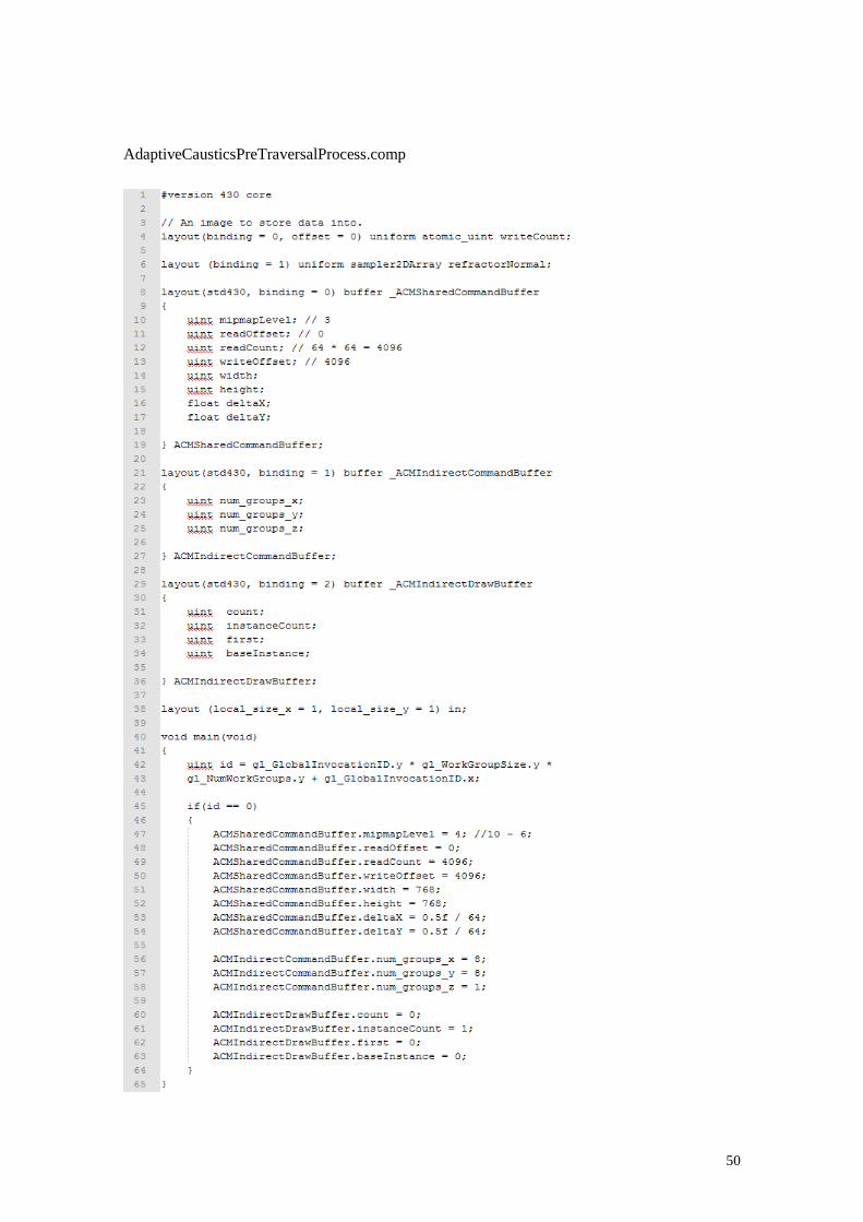
AdaptiveCausticsPreTraversalProcess.comp

51

AdaptiveCausticsTraversal.comp

Part 1:

52

AdaptiveCausticsTraversal.comp

Part 2:

53

AdaptiveCausticsPostTraversalProcess.comp

Part 1:

54

AdaptiveCausticsPostTraversalProcess.comp

Part 2:

55

AdaptiveCausitcsDrawDebug.comp

56

CausticsSplat.vert

Part 1:

57

CausticsSplat.vert

Part 2:

58

CausticsSplat.vert

Part 3:

59

CausticsSplat.vert

Part 4:

60

CausticsSplat.frag

Part 1:

61

CausticsSplat.frag

Part 2: