YITP-SB-15-??

AdS/CFT

Christopher P. Herzog

C. N. Yang Institute for Theoretical Physics, Department of Physics and Astronomy

Stony Brook University, Stony Brook, NY 11794

Abstract

A write up of about ten lectures on the AdS/CFT correspondence given as part of a second

semester course on string theory.

Contents

1 Preliminary Remarks 1

2 Why AdS/CFT might be true 2

2.1 Decoupling from the open string point of view . . . . . . . . . . . . . . . . . . . . . . 2

2.2 Decoupling from the closed string point of view . . . . . . . . . . . . . . . . . . . . . 3

2.3 Making a correspondence . . . . . . . . . . . . . . . . . . . . . . . . . . . . . . . . . 6

3 How AdS/CFT works 9

3.1 Scalar Two-Point Functions in Pure AdSd+1 . . . . . . . . . . . . . . . . . . . . . . . 13

3.2 Gauge fields in the bulk, global symmetries in the boundary . . . . . . . . . . . . . . 14

3.3 The stress tensor . . . . . . . . . . . . . . . . . . . . . . . . . . . . . . . . . . . . . . 15

4 A Basic Check of AdS/CFT 19

4.1 The Long Version . . . . . . . . . . . . . . . . . . . . . . . . . . . . . . . . . . . . . . 19

4.2 An Aside on N = 1 theories . . . . . . . . . . . . . . . . . . . . . . . . . . . . . . . . 26

5 Trace Anomalies 26

6 Hawking-Page Phase Transition 33

7 Current-Current Correlation Functions and Conductivity 38

8 Viscosity 41

9 Entanglement Entropy 45

A Bosonic Supergravity Actions and Equations of Motion 49

A.1 Type IIA . . . . . . . . . . . . . . . . . . . . . . . . . . . . . . . . . . . . . . . . . . 49

A.2 Type IIB . . . . . . . . . . . . . . . . . . . . . . . . . . . . . . . . . . . . . . . . . . 50

A.3 M theory . . . . . . . . . . . . . . . . . . . . . . . . . . . . . . . . . . . . . . . . . . 51

B Anti-de Sitter Space Metrics 51

C Supersymmetries of the type IIB D3-brane solution 53

1 Preliminary Remarks

The original AdS/CFT correspondence is the equivalence of type IIB string theory in a AdS5 × S5

background and maximally supersymmetric SU(N) Yang-Mills theory. (AdS stands for Anti-de Sit-

ter space and CFT for conformal field theory.) The conjectured equivalence was argued for, in large

part on the basis of symmetry, in the extraordinarily well cited 1997 paper [1] by Juan Maldacena.

Two critical follow up papers, one by Steve Gubser, Igor Klebanov, and Alexander Polyakov [2]

1

and another by Edward Witten [3] opened up the field by showing how the correspondence could

be usefully employed in the calculation of correlation functions. It should be emphasized that Mal-

dacena’s 1997 paper did not emerge from the vacuum. Like Athena and the head of Zeus, there

is a backstory; the one here involves calculations by Igor Klebanov and collaborators of strings off

D-branes and gravitons off of black holes. See for example [4].

These lecture notes are heavily influenced by earlier reviews on the subject. Two important ones

are by Maldacena, Aharony, Gubser, Ooguri, and Oz (MAGOO) [5] and by D’Hoker and Freedman

[6]. I begin by fleshing out an argument in the MAGOO review, explaining why AdS/CFT might

be true. Section 2 is in a weak and vague sense a distillation of the follow-up papers [2] and [3] and

explains the central calculational mechanism behind the correspondence. In Section 3, we perform a

basic check of the original correspondence between maximally supersymmetric Yang-Mills and type

IIB string theory in a AdS5 × S5 background – matching the Kaluza-Klein spectrum on the string

side to a set of protected operators on the gauge theory side. The rest of of the review contains

various important examples. We explain how to calculate two-point functions of scalar fields. We

explore the trace anomaly. We examine the phase diagram as a function of temperature of maximally

supersymmetric Yang-Mills on a sphere. We calculate the viscosity of maximally supersymmetric

Yang-Mills.

2 Why AdS/CFT might be true

The typical motivation for the AdS/CFT correspondence (or more generally gauge/gravity duality)

begins with a consideration of type IIA or IIB superstring theory. (We could also rephrase the

following discussion using the less well understood M-theory, but for simplicity we stick to ten

dimensions in what follows.) Consider a stack of N Dp-branes where the distance between the

branes is much less than the string length scale `s. There are two types of excitations: open strings

that live on the branes and closed strings that live in the bulk. Because of the condition on the

distance between the branes, the open strings can be nearly massless.

2.1 Decoupling from the open string point of view

We would now like to consider, in very general terms, a low energy effective field theory description of

the situation. In particular, we require that the energies E 1/`s are small compared to the string

scale. Only the massless strings can be excited. The closed string sector reduces to ten dimensional

supergravity, while the open string sector yields a supersymmetric (SUSY) (p+1) dimensional gauge

theory living on the stack of branes. We may also in principle try to allow for interactions between

these sectors:

S = Sclosed + Sopen + Sint . (1)

We now argue that these interactions must be irrelevant in the sense of the renormalization group,

and that at low energies Sclosed and Sopen decouple.

2

The Einstein-Hilbert term in the supergravity action is the usual

1

2κ2

∫ √−gR d10x , (2)

from which we see that dimensionally [κ] ∼ `4s. The gauge kinetic term in the gauge theory is the

standard

1

4e2

∫ √−g trF 2 dp+1x , (3)

from which we find that [e] ∼ `(p−3)/2s . (Note that we have recovered the usual fact that in 3+1

dimensions, gauge theories are classically scale invariant. One loop corrections of course can make e

run with scale.) To see how κ and e enter into Sint, we first perform the rescaling gµν → gµν +κhµν

and Aµ → eAµ. A term in Sint will take the schematic form

γ

∫dp+1x (κh)`(eA)m(∂)n (4)

where ∂ is a derivative. Thus the interaction must scale as

[γ] ∼ `−p−1+m+ns .

The physical coupling is not γ but γ = γκ`em which scales instead as

[γ] ∼ `−p−1+m+n+4`+m(p−3)/2s

∼ `(m2 −1)(p−1)+(n−2)+4`

s . (5)

We would like to argue that the exponent can never be negative. For the term to be an interaction,

certainly either (m ≥ 1 and ` ≥ 2) or (m ≥ 2 and ` ≥ 1). The worst case, i.e. most relevant, scenario

is n = 0, ignoring issues of gauge and diffeomorphism invariance which anyway would only force us

to choose a larger value of n. Thus we should check the two worst case scenarios: a) m = 1, ` = 2,

and n = 0; and b) m = 2, ` = 1, and n = 0. Choosing larger values of m, ` and n will just make

γ more irrelevant. In case (a), [γ] ∼ `6−(p−1)/2s which is irrelevant provided p < 13 which is always

true for ten dimensional string theories. In case (b), [γ] ∼ `2s which is always irrelevant.1

We should of course be more careful and look at the supersymmetric partners of the graviton

and the gauge field. One might worry that interactions between some of these partner fields might

be relevant and affect the low energy dynamics. We claim they do not and that in the low energy

limit Sint is effectively zero. Thus Sopen and Sclosed decouple.

2.2 Decoupling from the closed string point of view

We now change our perspective to a purely closed string point of view. After all open strings

traveling between D-branes can equally well be thought of as closed strings exchanged between the

D-branes. Martin Rocek in his lectures described a set of p-brane solutions in type IIA and IIB

1We are tacitly excluding D0-branes in this discussion, where we do not have a dynamical gauge field anyway.

3

supergravity. These solutions preserve 16 of the 32 supercharges and describe the back reaction of

the geometry and RR-fields to the presence of a stack of N Dp-branes. These p-brane solutions

satisfy the equations of motion that follow from the following gravity action

S =1

(2π)7`8s

∫d10x

√−γ[e−2Φ(R+ 4(∇Φ)2)− 1

2|Fp+2|2

]. (6)

where Fp+2 = dAp+1 and γµν is the string frame metric.2 (See Appendix A for the bosonic pieces

of the type IIA and IIB supergravity actions.) As this action is in string frame, the dilaton kinetic

term has the wrong sign. We introduce a fluctuation field φ such that eΦ = gseφ and rescale the

metric gµν = e−φ/2γµν . Under this rescaling, the Ricci scalar transforms as

R[γµν ] = e−φ/2[R[gµν ]− 9

2∇2φ− 9

2(∇φ)2

]. (7)

We deduce the following Einstein frame action

S =1

(2π)7g2s`

8s

∫d10x

√−g[R− 1

2(∇φ)2 − 1

2g2se

(3−p)φ/2|Fp+2|2], (8)

which now has a canonically normalized kinetic term for the dilaton field φ. The equations of motion

that follow from this action are

d ?e(3−p)φ/2Fp+2 = 0 , (9)

∇2φ =3− p

2g2se

(3−p)φ/2|Fp+2|2 , (10)

Rµν −1

2gµνR =

1

2(∂µφ)(∂νφ) +

1

2(p+ 1)!e(3−p)φ/2g2

sFµρ1···ρp+1Fνρ1···ρp+1

− 1

4gµν

((∇φ)2 +

e(3−p)φ/2

(p+ 2)!g2sFρ1···ρp+2F

ρ1···ρp+2

). (11)

The p-brane causes the metric to back react into the form

ds2 = H(p−7)/8

(−dt2 +

p∑i=1

dx2i

)+H(p+1)/8

9−p∑a=1

dy2a . (12)

The dilaton and RR potential are

eφ = H(3−p)/4 ; gsFp+2 = dt ∧ dx1 ∧ · · · ∧ dxp ∧ dH−1 . (13)

where H is a harmonic function (∇2H = 0). When the N Dp-branes are coincident, the harmonic

function takes the form

H(r) = 1 +

(L

r

)7−p

, r2 = ~y 2 . (14)

Although the factor of 1 in H(r) is not needed to have a solution, we include it so that the metric

becomes flat R1,9 in the limit r →∞ (far from the Dp-branes).

The quantity L should reflect the number of Dp-branes somehow. It follows from the definitions

that

e(3−p)φ/2 ? Fp+2 =1

gs(7− p)L7−p dvol(S8−p) , (15)

2In our conventions p!|Fp|2 = Fµ1···µpFµ1···µp .

4

where, thinking of the R9−p coordinatized by the ya as R+ × S8−p, dvol(S8−p) is the volume form

on the S8−p. Note that the funny factor of e(3−p)φ/2 would disappear in string frame. The first few

editions of Polchinski contain some mistakes regarding the Dp-brane quantization condition although

the discussion there is well worth reading. From (5) of ref. [7], we have that the RR field strength

should be quantized such that∫S8−p

e(3−p)φ/2 ? Fp+2 = (2π`s)7−pN . (16)

This quantization constraint tells us that L and N are related:

L7−p =(2π`s)

7−pgsN

(7− p) Vol(S8−p)= (4π)(5−p)/2Γ

(7− p

2

)`7−ps gsN . (17)

As we will use it greatly in what follows, we note that for the D3-brane, (L/`s)4 = 4πgsN .

The equations of motion are straightforward to check. From the Hodge dual expression (15), it

is clear that Fp+2 satisfies the first equation of motion (9). Using the fact that ∇2H = 0, it is also

straightforward to check the second equation of motion (10). We check only the trace of Einstein’s

equations (11):

2R = (∇φ)2 + (3− p)e(3−p)φ/2g2s |Fp+2|2 . (18)

From the form of the metric, we can compute that

R = −p+ 1

8

∇2H

H+

(p+ 1)(p− 3)

32

(∇H)2

H2, (19)

where the first term on the right hand side must vanish because H is harmonic. Using the dilaton

equation of motion (10) to replace |Fp+2|2, it is straightforward to check that the equation (18) is

satisfied. In appendix A, we give the bosonic pieces of the supergravity actions in ten and eleven

dimensions. We leave it as an exercise to the reader to verify that the Dp-brane solution above also

satisfies the type IIA and IIB equations of motion.

Given this Dp-brane solution, we can make an argument that the small and large r regions

decouple in a low energy limit. From the point of view of an observer at r = ∞, there are two

types of low energy excitations. The first are those at large r which locally have low energy. The

second are those at small r which locally can have any energy but because of the red-shift factor are

perceived by the observer at r = ∞ to have low energy. The red-shift factor is given by the time

component of the metric√−gtt(r) = H(r)(7−p)/16. Energies observed at different radii are related

via

E(r1)√−gtt(r1) = E(r2)

√−gtt(r2) . (20)

In particular, for the observer at r = ∞, we find that E(∞) = E(r)H(r)(p−7)/16. As r → 0 (and

provided p < 7), E(∞) becomes much, much less than E(r).

Now small r excitations have a difficult time to get to large r. The warp factor H(r) acts like

a gravitational well, as we can see by studying time-like geodesics traveled by a massive particle.

5

Suppose we try to throw a massive particle directly up from some small value of r. The part of the

line element that concerns us is (assuming p < 7)

ds2 = −H(p−7)/8dt2 +H(p+1)/8dr2 . (21)

To find the geodesic, we consider the equation of motion that follows from the following action

S = −m∫

dt√H(p−7)/8 −H(p+1)/8r2 . (22)

As the action does not depend explicitly on time, there is a conserved energy

E

m=H(p−7)/16

√1−Hr2

. (23)

If we start with a massive particle at a radius r L and some initial upward radial velocity r,

then the particle will eventually come to rest and start falling back down at a maximal radius given

by H(rmax) = (m/E)16/(7−p). For energies E m, this maximal radius will satisfy the inequality

rmax L.

Not only do excitations at small radius have trouble escaping to large radius, but large radius

excitations typically will not fall into the gravitational well and end up at small radius. One can

calculate the cross-section for these excitations. As the cross-section should scale perturbatively as

the gravitational coupling squared, we find that σ ∼ `8s. We should measure the cross section with

respect to directions transverse to the Dp-brane and the radial direction. Thus dimensionally we

expect that [σ] ∼ `10−p−2s . By dimensional analysis then we find that σ ∼ Ep`8s. As the energy E

goes to zero, the cross-section will go to zero as well. (See ref. [4] for a more careful calculation.)

2.3 Making a correspondence

From both the open and closed string description of the Dp-branes, there is a sector of the theory

which corresponds to ten dimensional supergravity in flat space. From the open string point of

view, we called this sector Sclosed. From the closed string point of view, this sector was the large r

region of our Dp-brane gravity solution. Given that the interactions between Sclosed and Sopen were

irrelevant from the open string point of view and also given that the large r and small r regions of

our Dp-brane gravity solution do not interact, we are naturally led to conjecture that Sopen and the

small r region of the Dp-brane gravity solution describe the same physics.

The case of D3-branes is special. Consider the behavior of the Ricci scalar curvature (19) at

small r. Plugging in H(r), we find that in every dimension except p = 3 (where it vanishes exactly)

R ∼ r−(p−3)2/8 diverges in the r → 0 limit, signaling the need for higher curvature corrections. A

second problem is associated with the dilaton. In the case where p < 3, the dilaton diverges in

the limit r → 0, indicating that the effective string coupling is diverging and signaling the need for

higher stringy corrections. These facts single out p = 3. In all other cases, the gravity solution

will need to be corrected in the small r region of the geometry, either because of gs corrections,

curvature corrections, or both. Indeed, we will see soon that the r → 0 limit for p = 3 is smooth

and innocuous.

6

Given the need for curvature and stringy corrections when p 6= 3, it is most natural to focus

henceforth on the case p = 3. The small r L region of the D3-brane solution has the line element

ds2 =r2

L2(−dt2 + d~x2) + L2 dr2

r2+ L2dΩ2

5 , (24)

where L4 = 4πgsN`4s. The line element dΩ2

5 gives the metric on a unit S5. The remaining pieces

of the metric describe the so-called Poincare patch of five dimensional anti-de Sitter space, AdS5,

a smooth homogenous space with no singularities. (See appendix B for various other coordinate

systems on AdS and their corresponding metrics.) The constant L is radius of curvature of both

the S5 and the AdS5. To stay out of the stringy regime, we need that this curvature scale should

be large compared to the string length, L `s which in turn implies that gsN 1. To keep the

string coupling small, we also need that gs 1. In most of the calculations we will use a slightly

different radial coordinate z = L2/r, for which the line element takes the more compact form

ds2 = L2

[−dt2 + d~x 2 + dz2

z2+ dΩ2

5

]. (25)

Including the one in H(r), the original D3-brane solution preserved 16 of the 32 supersymmetries

of type IIB supergravity. See appendix C for details. In the near horizon limit, we recover the lost

16, for a total of 32. (On the field theory side of the correspondence, this doubling comes from the

fact that the gauge theory is conformal.) The AdS5 has an SO(2,4) isometry group, which is the

conformal group for a field theory in R1,3. The sphere S5 has an SO(6) = SU(4)/Z2 isometry group.

This group is the global R symmetry group of a field theory with N = 4 supersymmetry in R1,3.

For an expert, Sopen could only be one thing. The N = 4 SUSY gauge theory in R1,3 is unique up

to choice of gauge group, and it’s conformal. The “obvious” choice of gauge group is U(N) for a

stack of N D3-branes without orientifolds.3

There is also an obvious choice for the identity of the gauge coupling and theta angle in the field

theory. Both N = 4 SU(N) Yang-Mills and type IIB supergravity are invariant under an SL(2, Z).

See appendix A for the details of the type IIB transformation rules. On the Yang-Mills theory, we

have

τ =θ

2π+

4πi

g2YM

, (26)

while on the type IIB SUGRA side we have

τ = C0 + ie−Φ . (27)

Both transform according to the rule

τ → τ ′ =aτ + b

cτ + d, (28)

3There is a subtle issue here of U(N) vs. SU(N). They are related by a U(1) subgroup. It is often said that the

diagonal U(1) corresponds to the center of mass degree of freedom of the stack and decouples from the other degrees

of freedom.

7

where ad− bc = 1. This coincidence suggests the identifications4

g2YM = 4πgs , θ = 2πC0 . (29)

A more careful calculation involving the DBI action of a couple of probe D3-brane bears out these

identifications.

SD3=− 1

(2π)3`4s

∫d4ξTrf

e−Φ[− det(Gab +Bab + 2π`2sFab)]

1/2

+1

(2π)3`4s

∫Trf [exp(2π`2sF2 +B2) ∧

∑q

Cq] + . . . (30)

= . . .− 1

(2π)3`4s

∫d4ξTrfe

−Φ (2π`2s)2

4FabF

ab

+1

(2π)3`4s

∫Trf

(2π`2s)2

2C0F2 ∧ F2 + . . . (31)

= . . .+

∫d4ξ

1

8πeΦ

1

2FαabF

αab +1

4π

1

2

∫d4ξ C0F

αabF

αcdε

abcd 1

4+ . . . (32)

The factors of 1/2 in the last line come from the trace in the fundamental representation Trf .

To recap, we have found a gravitational D3-brane solution which should describe N = 4 SUSY

Yang-Mills in a particular parameter regime. To avoid gravitational and stringy corrections, we

required that gsN 1 and gs 1. On the gauge theory side, these constraints mean that the

’t Hooft parameter λ = g2YMN = 4πgsN , which controls the perturbative expansion of the gauge

theory, must be taken large compared to one. Also to keep gs 1, we must take a large N limit,

N 1, on the gauge theory side.

The discussion of massive geodesics and black hole cross sections in the Dp-brane spacetime

foreshadows the identification of the radial coordinate as an energy scale in the field theory. If we

for the moment assume this identification is correct, we can interpret the behavior of the Ricci scalar

R and the dilaton Φ in string frame in the cases where p 6= 3. Unlike the Einstein frame discussed

above, in string frame

R =(3− p)(1 + p)

4

(∇H)2

H2

only diverges in the limit r → 0 when p > 3. Thus one could interpret the divergence in R for p < 3

in Einstein frame as really coming from the string coupling. Take p < 3, where the gauge coupling

becoming strong at low energies mirrors the fact that the dilaton blows up at small r. Having thrown

away the one in H to take the near horizon limit, the Ricci scalar blows up at large r, indicating the

need for higher curvature corrections, suggesting that the ’t Hooft coupling is getting weak at high

energies. Correspondingly when p > 3, we have the opposite situation. Having thrown away the one

in H, the dilaton blows up at large r, corresponding to the fact that the effective gauge coupling

gets large at high energy. The Ricci scalar now blows up at small r, signaling the need for higher

curvature corrections and suggesting that the ’t Hooft coupling has become small at low energies.

4There seem to be some disagreements in the literature regarding the constant of proportionality relating g2YM and

gs. For example the relation in the review [6] does not include the factor of 4π.

8

3 How AdS/CFT works

The equivalence of N = 4 SYM and type IIB string theory in AdS5 × S5 should imply an equality

between their respective path integrals. On the the gauge theory side, we ought to be able to

include gauge invariant sources in the path integral. On the gravity side, AdS5 is a space with

boundary (at z = 0 in the parametrization (25)). Thus to be well defined, we need to include

boundary conditions. Consider probing the stack of D3-branes with wave packets sent in from the

asymptotically flat part of the D3-brane geometry. From the near horizon point of view, these

wave packets look alternately like sourcing gauge invariant operators on the D-branes or like setting

boundary conditions for the AdS5 space-time. This line of reasoning leads to the central postulate

of the AdS/CFT correspondence, a result [2, 3] whose importance can not be over emphasized:

eWCFT[φ0] ≡⟨

exp

∫d4xφ0(x)O(x)

⟩CFT

= Zstring

[φ(x, z)|z→0 = φ0(x)

]. (33)

In this expression φ(x, z) is a field on the string side of the story. Its boundary value φ0(x) can

alternately be interpreted as a source for a gauge invariant operator O(x) in the conformal field

theory. The CFT quantity WCFT is then a generating functional for connected correlation functions

of O(x) in the CFT.

While the correspondence (33) is expected to hold true in general, we will be interested in it

primarily in the limit gs and `s/L → 0. In field theory terms, this double limit is g2YMN and

N →∞. Given that we are working in AdS5 with a scale set by the radius of curvature L, we can

first replace Zstring by the corresponding supergravity partition function ZSUGRA. Then the effective

gravitational coupling constant in the supergravity action (8) we can identify as

(2π)7g2s`

8s

L8=

8π2

N2Vol(S5) . (34)

Because N is large, a saddle point approximation of ZSUGRA ∼ e−Sos becomes accurate. (We work

in Euclidean signature here.) In other words, the on-shell gravitational action Sos[φ0] (i.e. the action

evaluated using the equations of motion) is a good approximation to the generating functional,

WCFT[φ0] ≈ −Sos[φ0]. We can therefore use classical gravity to compute connected correlation

functions in the CFT in the limit N →∞.

We would like to explore the consequences of the postulate (33) for a free scalar field. Consider

then the action for a real scalar in the Poincare patch of (Euclidean) AdSd+1:

S =1

2

∫dd+1x

√−g[(∂φ)

2+m2φ2

]. (35)

We focus here just on the AdSd+1 geometry and use the line element

ds2 = L2

[δµνdxµdxν + dz2

z2

]. (36)

To produce a generating function for the CFT correlation functions, we need to evaluate this action

on-shell with a prescribed boundary condition for φ at z = 0. To that end, let us start with the

9

equation of motion for φ:

(zd+1∂zz

−d+1∂z + z2ηµν∂µ∂ν −m2L2)φ = 0 . (37)

Typically boundary conditions for second order differential equations are either Dirichlet or Neu-

mann. Here, however, z = 0 is a singular point, and the boundary behavior is described instead by

two characteristic exponents which satisfy the following indicial equation:

∆(∆− d) = m2L2 , (38)

as can be seen by plugging φ ∼ z∆ into the equation of motion (37) and expanding the result near

z = 0. Generically, one finds the following behavior for φ near z = 0:

φ = azd−∆(1 +O(z2)) + bz∆(1 +O(z2)) . (39)

(Interesting issues arise when ∆ is an integer and the series overlap. Extra logarithmic terms appear

which we shall ignore.) If we assume ∆ > d/2, then a describes the leading small z behavior and

we can tentatively identify a = φ0 with the source term in the CFT. The singular behavior at z = 0

means we should really work with a z = ε cutoff and modify the basic statement (33) to include an

ε dependence, φ|z=ε = φ0εd−∆, taking the ε→ 0 limit only at the end.

Given that the boundary z = 0 is a singular point and we cannot use typical Dirichlet or Neumann

boundary conditions, it is not obvious that the action (35) has a well defined variational principle.

In varying the action, we are left with the following boundary term

δS = −∫z=ε

ddx

(L

z

)d−1

δφ(x, z)∂zφ(x, z) (40)

= −Ld−1

∫z=ε

ddx1

zd(δa zd−∆ + δb z∆ + . . .)(a(d−∆) zd−∆ + b∆ z∆ + . . .)

= −Ld−1

∫z=ε

ddx[(d−∆)a δa zd−2∆ + (∆ δa b+ (d−∆) δb a)

+∆ b δb z2∆−d + . . .].

There are really three potentially overlapping power series in the last line. The boundary variation

(40) includes only the leading term in each power series; the ellipses denote the subleading terms. In

the context of the variational principle, we fix the boundary behavior a = φ0. Thus, we insist that

δa = 0. There remains a term proportional to δb a which we need to cancel through the addition of

a boundary term. (The b δb term will vanish given our assumption that 2∆ > d.) We add

Sbry =c

L

∫z=ε

ddx√−γ φ2(x, z) (41)

where γµν is the induced metric on the z = ε slice of the geometry, and c is a constant to be

determined. The choice of counter-terms is guided by the requirements that Sbry be local, Lorentz

invariant, and depend only intrinsically on the geometry of the boundary. One could imagine also

terms of the form φφ and φ2φ where = ηµν∂µ∂ν or even, in the case of a curved boundary,

10

Rφ2 where R is the Ricci scalar curvature of the boundary. By dimensional analysis, these higher

derivative terms must come with additional powers of z and cannot cancel the leading a δb term.

Given the boundary term (41), the variation is then

δSbry = 2cLd−1

∫z=ε

ddx[a δa zd−2∆ + (a δb+ b δa) + b δb z2∆−d + . . .

], (42)

To cancel the a δb term in (40), we should set the constant c = (d−∆)/2.

Having ensured that the on-shell value of the action is indeed an extremum, and thus that the

saddle-point approximation is sensible, we can ask what the response of the system is to small

changes δa in the source term. The calculation is essentially already done. The leading a δa term

cancels and one finds

δStot = δS + δSbry = Ld−1

∫z=ε

ddx (d− 2∆)b δa . (43)

The expectation value of the operator dual to φ then follows from the basic postulate (33):

〈O〉 = −δStot

δφ0= −δStot

δa= Ld−1(2∆− d) b . (44)

We have come to a second omission in the discussion. The ellipses in the variations (40) and

(42) contain subleading terms in the a δa series which may be dominant compared to the b δa term

considered in (43). In general, we require further counter-terms to cancel these subleading a δa pieces

and to prevent 〈O〉 from being UV divergent. As an example, one may consider the subleading term

in the a δa series, proportional to zd−2∆+2δaa. Assuming 2∆ > d + 2, this term is dominant

compared to b δa, but it can be canceled by adding a φφ boundary term to the action. That these

counterterms can be identified in general and that 〈O〉 can be renormalized is discussed in more

detail in for example ref. [8]. The procedures described above for scalar fields can be generalized for

higher spin fields. These techniques usually go by the name of “holographic renormalization”.

Note that the characteristic exponent ∆ is also the scaling dimension of the operator O. The

transformation rule x→ Λx and z → Λz is a symmetry of the line element (36) and of the geometry

of AdSd+1. The restriction of the scaling symmetry to the boundary z = 0 corresponds to scale

transformations of the CFT. Under this scale transformation, the field φ transforms as φ′(z, x) =

φ(Λz,Λx). Thus we find that

〈O′〉 = Λ∆〈O〉 . (45)

Primary scalar operators in CFT satisfy a unitarity bound [9], ∆ > (d− 2)/2, saturated by the

free field case. The assumption ∆ > d/2 thus leaves out a set of operators with scaling dimension

in the range (d − 2)/2 < ∆ < d/2. To close this gap, let us now assume that ∆ < d/2 and repeat

the exercise we went through above. We still freeze the value of a and thus set δa = 0. Now, in

addition to canceling the a δb term in the variation (40), we also need to cancel the b δb term, which

no longer vanishes in the limit z → 0. Breaking from our rule that counterterms should depend only

on the intrinsic geometry of the boundary, we add a Gibbons-Hawking like term that depends on a

11

-

( )

-

Δ

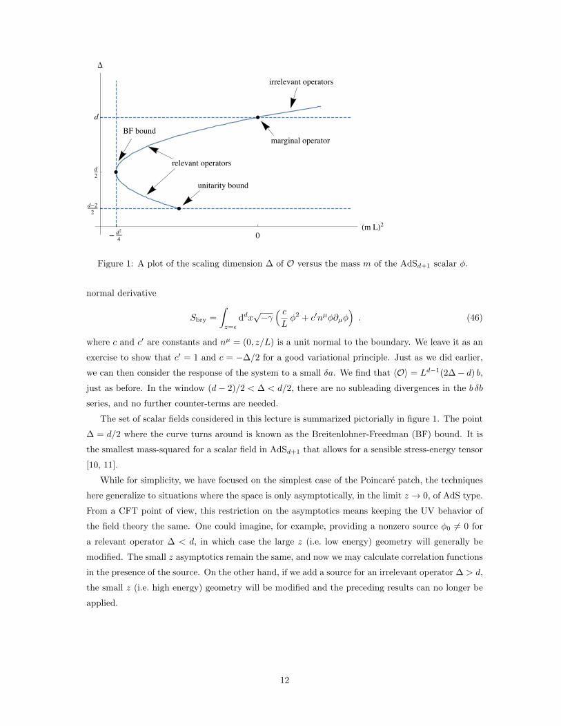
Figure 1: A plot of the scaling dimension ∆ of O versus the mass m of the AdSd+1 scalar φ.

normal derivative

Sbry =

∫z=ε

ddx√−γ( cLφ2 + c′nµφ∂µφ

). (46)

where c and c′ are constants and nµ = (0, z/L) is a unit normal to the boundary. We leave it as an

exercise to show that c′ = 1 and c = −∆/2 for a good variational principle. Just as we did earlier,

we can then consider the response of the system to a small δa. We find that 〈O〉 = Ld−1(2∆− d) b,

just as before. In the window (d− 2)/2 < ∆ < d/2, there are no subleading divergences in the b δb

series, and no further counter-terms are needed.

The set of scalar fields considered in this lecture is summarized pictorially in figure 1. The point

∆ = d/2 where the curve turns around is known as the Breitenlohner-Freedman (BF) bound. It is

the smallest mass-squared for a scalar field in AdSd+1 that allows for a sensible stress-energy tensor

[10, 11].

While for simplicity, we have focused on the simplest case of the Poincare patch, the techniques

here generalize to situations where the space is only asymptotically, in the limit z → 0, of AdS type.

From a CFT point of view, this restriction on the asymptotics means keeping the UV behavior of

the field theory the same. One could imagine, for example, providing a nonzero source φ0 6= 0 for

a relevant operator ∆ < d, in which case the large z (i.e. low energy) geometry will generally be

modified. The small z asymptotics remain the same, and now we may calculate correlation functions

in the presence of the source. On the other hand, if we add a source for an irrelevant operator ∆ > d,

the small z (i.e. high energy) geometry will be modified and the preceding results can no longer be

applied.

12

3.1 Scalar Two-Point Functions in Pure AdSd+1

Above, in expanding the field φ(x, z) near the boundary

φ(x, z) = zd−∆a(1 + . . .) + z∆b(1 + . . .)

and positing a = φ0, we found that the one-point function 〈O〉 ∼ b was determined by the coefficient

of the second series. Here, we will use a second boundary condition to find a relation between b and

the source a. Given that relation, we can then compute a two-point correlation function 〈OO〉 by

varying 〈O〉 with respect to a = φ0.

In pure AdSd+1, we can find an explicit solution of the equations of motion (37) for the scalar

field. We first make a plane wave ansatz, φ ∼ ek·xφ(z). The equation of motion simplifies to an

ordinary differential equation

zd+1(z1−dφ′)′ − (z2k2 +m2L2)φ = 0 , (47)

where ′ denotes ∂z. Next, we make the substitution φ(z) = zd/2H(z),

z2H ′′ + zH ′ −(k2z2 +m2L2 +

d2

4

)H = 0 , (48)

and recognize a second order differential equation of Bessel type. In the Euclidean or space-like case

where k2 > 0, we find a solution in terms of Hankel functions:

H = c1H(1)ν (ikz) + c2H

(2)ν (ikz) , (49)

where we have defined ν ≡√m2L2 + d2/4. To fix the second boundary condition, consider the large

z behavior where H(1)ν (ikz) ∼ e−kz and H

(2)ν (ikz) ∼ ekz, allowing us to set c2 = 0 and throw out

the second, exponentially growing solution.

To extract the two-point function, consider the small z expansion of the solution, assuming

∆ > d/2 and that ν is not an integer,

φ = c1

[zd−∆

(− iπ

(2

ik

)νΓ(ν) + . . .

)+ z∆

((ik

2

)ν1 + i cot(πν)

Γ(1 + ν)+ . . .

)]. (50)

From the leading and subleading coefficients of the series expansion, we can read off the values of

φ0 and 〈O〉:

φ0 = c1

(− iπ

)(2

ik

)νΓ(ν) , (51)

〈O〉 = (2∆− d)Ld−1c1

(ik

2

)ν1 + i cot(πν)

Γ(1 + ν). (52)

The (Fourier transform of the) two-point function can then be extracted by varying the one-point

function:

GOO(k) =δ〈O〉δφ0

=〈O〉φ0

= (−2ν)

(ik

2

)2ν

(iπ)1 + i cot(πν)

Γ(ν)Γ(1 + ν)Ld−1 (53)

13

We need now to Fourier transform back to position space. Focusing on the k2ν = k2∆−d behavior,

note that by translational symmetry and dimensional analysis, the only possible result is that

〈O(x2)O(x1)〉 =

∫ddk

(2π)dGOO(k)eik·(x2−x1) ∼ 1

|x2 − x1|2∆. (54)

Two-point functions in CFT are indeed constrained to have precisely this form.

3.2 Gauge fields in the bulk, global symmetries in the boundary

Having gained some experience with scalar fields, we move on to gauge fields in AdSd+1, which

in the context of the holographic renormalization are actually somewhat simpler, requiring fewer

counter-terms. Consider the following abelian gauge field in the bulk:

S = − 1

4e2

∫dd+1x

√−gFABFAB . (55)

The equations of motion are simply ∂A√−gFAB = 0. To keep the discussion simple, we pick a

radial gauge Az = 0. The equations of motion ∂A√−gFAµ expand, using the line element (36), to

give

∂zz3−d∂zAµ + z3−d∂λη

λνFνµ = 0 . (56)

In analogy to the scalar discussion, we consider a small z expansion of the gauge field, Aµ ∼ z∆.

The corresponding indicial equation

∆(∆ + 2− d) = 0 , (57)

has the two roots ∆ = 0 and ∆ = d− 2, leading to the following small z series solution

Aµ = aµ(1 + . . .) + bµzd−2(1 + . . .) . (58)

We should also consider the remaining equation of motion ∂A√−gFAz = 0 which expands to give

∂µz3−d∂zη

µνAν = 0 . (59)

Inserting the small z series solution into this equation of motion produces the constraint ∂µηµνbν = 0.

In other words, ηµνbν satisfies a current conservation condition.

In determining the equations of motion, we produced a boundary term which we now consider

more carefully:

δS =Ld−3

e2

∫z=ε

ddx z3−dηµνδAµ∂zAν (60)

=Ld−3

e2

∫z=ε

ddx z3−dηµν(δaµ + δbµ zd−2)((d− 2)bνz

d−3 + . . .) (61)

=Ld−3

e2

∫z=ε

ddx (d− 2)ηµνδaµ bν . (62)

To get a good variational principle, where we set δaµ = 0, we need no further counter-terms. To

extract the one-point function however, we may find that even though the leading a δa term cancels

14

because of the ∂z derivative, there could be subleading divergences that are nonetheless dominant

compared to the δa b term. In fact the situation here is further complicated by the fact that d − 2

is integer and the two series may overlap, generating logarithms. There is a z → −z symmetry of

the equations of motion which implies that the series expansion is in even powers of z. Thus, the

series only overlap when d is an even integer. While in d = 3, we may take the variation (62) at face

value, in d = 4 a logarithmic singularity appears which requires more careful treatment. In d > 4,

there can be further complications. Ignoring these gritty details, we take the variation (62) at face

value and compute the one-point function:

〈Jµ〉 =δS

δaµ=

(d− 2)Ld−3

e2ηµνbν . (63)

We are now in a position to identify the operator Jµ. From the point of view of the CFT, it is

sourced by an external gauge field aµ and satisfies a current conservation condition ∂µJµ = 0. Thus

it must be a conserved current. Note that aµ is not dynamical both from the gravity and CFT point

of view.

3.3 The stress tensor

The stress-tensor operator in the CFT is one of the more difficult fields to study through AdS/CFT

but also one of the most useful and interesting. It naturally couples to the boundary value of the

metric. To analyze this case, let us first set some notation. The bulk metric shall be GAB . We will

pick a gauge where the line-element is

ds2 =L2

z2dz2 + γµνdxµdxν , (64)

where γµν is the boundary metric. We further define

gµν ≡z2

L2γµν . (65)

In general, gµν will have a nontrivial z dependence which we can write for small z as

gµν =

g(0)µν + z2g

(2)µν + . . .+ zdg

(d)µν + zd+2g

(d+2)µν + . . . , odd d

g(0)µν + z2g

(2)µν + . . .+ zdg

(d)µν + zd log z h

(d)µν + . . . , even d

(66)

Note that the CFT metric is not gµν but the boundary value g(0)µν . The full tensor structure gµν

contains more information, as we will see.

Given the earlier discussion of scalars and gauge fields, we can anticipate that the action will

contain a bulk contribution, a boundary contribution to have a good variational principle, and

further counter-terms to render the correlation functions finite:

S = SEH + SGH + Sctr . (67)

The bulk term is Einstein-Hilbert plus a negative cosmological constant, required so that AdSd+1 is

a solution of the equations of motion:

SEH =1

2κ2

∫M

dd+1x√−G

(R+

d(d− 1)

L2

). (68)

15

However, anti-de Sitter space has a boundary and second derivatives R ∼ ∂2GAB in the action will

generate boundary terms of the form ∂A(δgBC) which need to be canceled. The standard procedure

is to add a Gibbons-Hawking term

SGH =1

κ2

∫∂M

ddx√−γK , (69)

where K = GAB∇AnB is the trace of the extrinsic curvature and nB is an outward pointing unit nor-

mal vector. Such a boundary term will cancel normal derivatives of the metric variation nA∂A(δgBC).

The variation of the Einstein-Hilbert term gives

δSEH =1

2κ2

∫M

dd+1x

[√−G(δRAB)GAB +

√−GRABδGAB +

(R+

d(d− 1)

L2

)δ(√−G)

]. (70)

The variation of the second two terms produces Einstein’s equation, which vanish on-shell. The

variation of the Ricci tensor is a covariant derivative

δRAB = −(δΓCAC);B + (δΓCAB);C , (71)

a result sometimes known as the Palatini identity. Inside the action, this variation becomes a total

derivative

√−GGABδRAB = −(

√−GGABδΓCAC),B + (

√−GGABδΓCAB),C (72)

Skipping some steps which we will flesh out in the next section, this total derivative reduces to the

boundary term

δSEH = − 1

2κ2

∫∂M

ddx√−γ(nAγCDδGCD;A −KnAnBδGAB +KABδGAB

). (73)

Meanwhile, varying the Gibbons-Hawking term leads to

δSGH =1

κ2

∫∂M

ddx[√−γ δK −K δ(

√−γ)

]. (74)

Again skipping some steps, the variation of the extrinsic trace produces

δK =1

2γCDδGCD;An

A − K

2nAnBδGAB .

Assembling the pieces, the boundary variation is then

δSEH + δSGH = − 1

2κ2

∫∂M

ddx√−γ(Kµν −Kγµν)δγµν (75)

where KAB = ∇(AnB). Thus the “bare” stress tensor will be5

(Tbare)µν√−g(0)

2=

δS

δg(0)µν

= −Ld+2

2κ2

√−g 1

zd+2(Kµν −Kγµν) . (76)

This stress tensor appears in the early AdS/CFT paper [12]. The factor of z−d−2 in this expression

suggests that the bare stress tensor may be divergent. Indeed, combined with an inverse metric

5In Lorentzian signature, conventionally the variation of the action is proportional to the stress tensor. In Euclidean,

there should be a relative minus sign. We are implicitly working in Lorentzian signature here.

16

factor γµν , there will in general be divergent terms starting at order z−d. These terms need to be

regulated. The form of the counter terms in d ≤ 6 is

Sctr =1

κ2

∫∂M

ddx√−γ[d− 1

L+

L

2(d− 2)R+

L3

(d− 4)(d− 2)2

(RµνRµν −

d

4(d− 1)R2

)+ . . .

]. (77)

The Ricci tensor Rµν is computed with the boundary metric γµν . We include as many of these

counter-terms as are necessary to cancel the divergences. A term of the form√−γRn can cancel a

divergence of order z−d+2n. As a result, we need to include counter terms up to but not including

O(Rd/2) to cancel potential divergences. (In even d, there is an ambiguity in the definition of

the stress tensor that comes from including terms of precisely O(Rd/2). This ambiguity parallels a

similar ambiguity on the the field theory side. In d = 4, for example, there is an analogous ambiguity

in the coefficient of the R term in the trace anomaly.) In AdS3, only the first term is needed. For

AdS4 and AdS5, the first and second are needed. The second term proportional to R can be thought

of as an analog of the φφ counter term we needed for the scalar field. For AdS6 and AdS7, all

three are needed, and higher order terms we have not written down would need to be constructed

to regulate the divergences in d > 6.

Deriving the Boundary Stress Tensor

Similar discussions to the following can be found in textbooks on general relativity, for example

appendix E.1 of Wald’s book. However, in most of the general relativity literature, the variation

of the metric on the boundary is set to zero, δGAB |z=0 = 0. Like in the the case of the scalar

we studied before, we would like to discover the response of the system to small variations in the

boundary value of δGAB . Thus we need to redo the classic textbook calculations, keeping a nonzero

value for the metric fluctuations on the boundary.

We begin by studying the term proportional to δRAB in the variation of the Einstein-Hilbert

action (70). Using that δRAB becomes a total derivative (72) inside the integral, the variation (70)

becomes

δSEH = − 1

2κ2

∫∂M

ddx√−γ[GABδΓCACnB −GABδΓCABnC

](78)

= − 1

2κ2

∫∂M

ddx√−γ GABGCD (δGCD;AnB − δGAD;BnC) (79)

= − 1

2κ2

∫∂M

ddx√−γ nAGCD (δGCD;A − δGCA;D) . (80)

We can write the boundary metric as an operator γAB = GAB − nAnB that projects onto the

subspace orthogonal to nA. In the variation, we can replace GCD with γCD as the terms proportional

to nAnCnD will drop out of the difference:

δSEH = − 1

2κ2

∫∂M

ddx√−γ nAγCD (δGCD;A − δGCA;D) . (81)

But now γCDδGCA;D becomes almost a total tangential derivative which we can integrate by parts.

In more detail, we have the identity

γED(γCDnAδGAC);E = −KnAnCδGAC +KACδGAC + γCDnAδGAC;D , (82)

17

where now the quantity on the left really is a total boundary derivative because the covariant

derivative acts on a quantity with projected indices. In this identity we have replaced the covariant

derivative of the unit normal with the extrinsic curvature, nA;C = KAC . This identity combined

with the intermediate result (81) leads to

δSEH = − 1

2κ2

∫∂M

ddx√−γ

(nAγCDδGCD;A −KnAnCδGAC +KACδGCA

). (83)

Next we consider the variation of the Gibbons-Hawking term:

δSGH =1

κ2

∫∂M

ddx(√−γ δK +Kδ(

√−γ)

). (84)

Rewriting δK in terms of the connection leads to

δK = (δ∇A)nA +∇AδnA .

The first term in this variation can be simplified straightforwardly:

(δ∇A)nA = (δ∇A)nA

= (δΓAAC)nC

=1

2GAD(δGAD;C + δGCD;A − δGAC;D)nC

=1

2GADδGAD;Cn

C .

The constraint nAnA = 1 implies that the variation of the unit normal must take the form

δnA =

(1

2nAn

BnC + cγBAnC

)δGBC , (85)

where c is an as yet undetermined constant. To fix c = 0, we know that the tangent vectors

∂XA/∂xµ do not depend on the metric and must be orthogonal to δnA. But to vary K, we need

δnA = δ(gABnB) which must then be

δnA = −(

1

2nAnBnC + γABnC

)δGBC . (86)

The variation of the trace of the extrinsic curvature is thus

δK =1

2γADδGAD;Cn

C − K

2nBnCδGBC −∇A(γABnCδGBC) . (87)

The variation of the Gibbons-Hawking term then becomes

δSGH =1

2κ2

∫∂M

ddx√−γ(nAγBCδGBC;A −KnAnBδGAB +KγABδGAB

), (88)

where we have discarded a total boundary derivative. As is well known, the normal derivatives in

δSEH and δSGH cancel. As is less well known, the terms proportional to KnAnBδGAB cancel as

well, leaving the boundary stress tensor (75).

18

4 A Basic Check of AdS/CFT

In this lecture, we perform a consistency check of the correspondence between N = 4 SU(N) SYM

and type IIB string theory in an AdS5 × S5 background. Recall the basic field content of N = 4

SYM. There is a gauge field Aµ, four Weyl fermions λi, and six real scalar fields φI , all transforming

in the adjoint of SU(N).

Previously, we learned of a series of scalar fields in the KK reduction of AdS5 × S5. These were

linear combinations of haa and Cabcd with all legs in the S5. They transformed in a symmetric

traceless representation of SO(6). Recall that SO(6) = SU(4)/Z2. In SU(4) languague, they have

the Young tableaux (0, p, 0) for p > 1:

, , , · · · (89)

We also saw that they had masses (mL)2 = p(p− 4).

We claim that the boundary values of these supergravity fields act as sources for traceless sym-

metric products of the φI of N = 4 SU(N) SYM, Op = tr(φI1 · · ·φIp)cI1···Ip where the tensor cI1···Ip

is symmetric and traceless. In the limit g2YMN → 0, the φI are free fields with scaling dimension

∆(φI) = 1. It then follows that ∆(Op) = p, consistent with the mass-scaling dimension relation (38).

But this argument is too fast. At this point, it is not at all clear why ∆(Op) should be independent

of g2YMN . There is a long story here, the short version of which follows directly. The full version

will take us some time.

The rough answer is that N = 4 SYM is a superconformal field theory. The superconformal

algebra (SCA) has two types of SUSY generators, call them S and Q, 16 of each. That Op is

a superconformal primary means that it is annihilated by the S. That Op belongs to a 1/2 BPS

multiplet implies that it is annihilated by half of the Q’s. The SCA has the anticommutation relation,

schematically,

Q,S = M +R+D , (90)

where M is a Lorentz generator, R is an R-symmetry generator, and D is a dilation operator, whose

eigenvalues are proportional to ∆. This anticommutation relation thus implies that the R-charge of

the scalar operator is proportional to the scaling dimension ∆. In other words, ∆ is protected by

the structure of the SCA. We have then a nontrivial check of the AdS/CFT correspondence.

4.1 The Long Version

The discussion in this section draws heavily from ref. [13].

The conformal group is the Poincare group extended by dilations and special conformal trans-

19

formations. The Lie algebra commutation relations are as follows:

[Pρ,Mµν ] = i(ηρµPν − ηρνPµ) , [Kρ,Mµν ] = i(ηρµKν − ηρνKµ) , (91)

[Mµν ,Mλρ] = i(ηνλMµρ + ηµρMνλ − ηµλMνρ − ηνρMµλ) , (92)

[D,Pµ] = iPµ , [D,Kµ] = −iKµ , [Kµ, Pν ] = −2iMµν + 2iηµνD , (93)

where Pµ generate translations, Mµν Lorentz transformations, Kµ special conformal transformations,

and D dilations. If the Poincare group acts on R1,d−1, then the conformal group is isomorphic to

SO(2,d), as can be seen by considering the linear combinations Pµ ±Kµ. In the context of 2d CFT

from last semester, we may identify the Virasoro generators L1 and L1 with linear combinations of

the Kµ; L−1 and L−1 with linear combinations of the Pµ; and L0 and L0 with D and the rotation

generator M01.

A standard differential operator representation of this algebra is

Mµν = i(xµ∂ν − xν∂µ) , (94)

Pµ = −i∂µ , D = −ixµ∂µ , (95)

Kµ = i(x2∂µ − 2xµxν∂ν) . (96)

Note that D has eigenvalues i∆ when acting on monomials in xµ of degree −∆.6

Toward the goal of studying superconformal primary operators, we review first the definition of

conformal primaries. Note from the relation (93) it follows that for eigenvectors of D, Pµ increases ∆

by one while Kµ lowers it by one. A conformal primary is a lowest weight state of D, or equivalently

a state annihilated by Kµ that is not Pµ of something else. (States that are Pµ of something else

we typically call descendants.) Let O(x) be a conformal primary operator and |O〉 = O(0)|0〉 the

corresponding conformal primary state. We have that

Kµ|O〉 = 0 , D|O〉 = i∆|O〉 . (97)

To define a superconformal algebra, we specialize to d = 4 dimensions and add the new generators

Qiα , Qiα , Siα , Siα , (98)

where i = 1, . . . , N and α, α = 1, 2. We will see in a moment that there are also R-symmetry

generators Rij . These additions yield the superconformal algebra su(2, 2|N). The anticommutation

6We have presented the conformal algebra in a way suggesting that all the generators are Hermitian, in which

case they should have real eigenvalues. It may seem strange then that the operator D can have a pure imaginary

eigenvalue. One comment is that D = −ixµ∂µ is not Hermitian with the usual inner product 〈u, v〉 =∫u(x)∗v(x) dx.

Another is that monomials in xµ of degree ∆ are not normalizable eigenvectors under this inner product anyway. A

third is that the group SO(2,4) is non-compact with a Lorentzian metric that is not positive definite.

20

relations among the ordinary supercharges Q and superconformal charges S are as follows:

Qiα, Qjα = 2δijPαα , Qiα, Qjβ = 0 = Qiα, Qjβ , (99)

Siα, Sjα = 2δijKαα , Siα, Sjβ = 0 = Siα, Sjβ , (100)

Qiα, Sjα = 0 , Siα, Qjα = 0 , (101)

Qiα, Sjβ = 4

[δij(Mα

β − i

2δβαD)− δβαRij

], (102)

Siα, Qjβ = 4

[δij(M

αβ

+i

2δαβD)− δα

βRij

], (103)

where we have defined

Pαα = (σµ)ααPµ , Kαα = (σµ)ααKµ , (104)

Mαβ = − i

4(σµσν) β

α Mµν , M αβ

= − i4

(σµσν)αβMµν . (105)

The most important relations here are eqs. (99), (100), (102) and (103). In the same way that the

ordinary supercharges Qiα and Qjβ function morally as the square root of the momentum generator

Pµ, in the superconformal extension of the super-algebra, Siα and Sjβ function as the square root

of the superconformal generator Kµ. In defining superconformal primary operators, this fact means

we can replace Kµ by Siα and Sjβ . One other thing to note: The anti-commutation relations (102)

and (103) are the precise version of the relation (90), to be used in the last and crucial step of

demonstrating that the Op are protected operators.

We then need also to specify how Qiα, Qjβ , Siα, and Sjβ fail to commute with the generators

of the conformal group:

[Mαβ , Qiγ ] = δβγQ

iα −

1

2δβαQ

iγ , [Mα

β , Siγ ] = − δγαSi

β +1

2δβαSi

γ , (106)

[M αβ, Qiγ ] = − δαγ Qiβ +

1

2δαβQiγ , [M α

β, Siγ ] = δγ

βSiα − 1

2δαβSiγ , (107)

[D,Qiα] =i

2Qiα , [D, Qiα] =

i

2Qiα , [D,Si

α] = − i

2Siα , [D, Siα] = − i

2Siα , (108)

[Kµ, Qiα] = − (σµ)ααS

iα , [Kµ, Qiα] = Siα(σµ)αα , (109)

[Pµ, Siα] = − (σµ)ααQiα , [Pµ, Si

α] = Qiα(σµ)αα . (110)

The most important relations here for us are eqs. (108). From these relations it follows immediately

that Qiα and Qjβ act to raise ∆ by 1/2, while Siα and Sjβ lower ∆ by 1/2. Superconformal primary

states, which are also lowest weight states of D, are annihilated by Siα and Sjβ and are not Qiα or

Qjβ of something else.

Finally, we need to specify how the R-symmetry generators act:

[Rij , Rkl] = δkjR

il − δilRkj , (111)

[Rij , Qkα] = δkjQ

iα −

1

4δijQ

kα , [Rij , Qkα] = − δikQjα +

1

4δijQkα , (112)

[Rij , Skα] = − δikSj

α +1

4δijSk

α , [Rij , Skα] = δkj S

iα − 1

4δijS

kα . (113)

21

If we take the R-symmetry generators to be traceless Rii = 0, replacing the R-symmetry group U(4)

with SU(4), then the superalgebra becomes psu(2, 2|4).

Now let us consider the SUSY transformations of the fields in N = 4 SYM. Recall that N = 4

SYM has six real scalar fields φI (I = 1, . . . , 6); four Weyl fermions λiα and λjα (i = 1, . . . , 4 and

α, α = 1, 2); and a gauge field Aµ, all transforming in the adjoint representation of the gauge group

G, which we here take to be SU(N). The R-symmetry group is SU(4). Thus the φI transform in

the defining representation of SO(6) (or equivalently an antisymmetric irreducible representation of

SU(4)). The λi and λj transform in the fundamental and antifundamental of SU(4) (or equivalently

spinor representations of SO(6)). The SUSY rules are as follows [6]:

δφI = [Qiα, φI ] = (CI)ijλjα , (114)

δλjβ = Qiα, λjβ = F+µν(σµν)αβδ

ij + [φI , φJ ]εαβ(CIJ)ij , (115)

δλjβ

= Qiα, λj

β = (CI)

ij(σµ)αβDµφI , (116)

δAµ = [Qiα, Aµ] = (σµ)αβλiβ. (117)

The CI and CIJ are constructed from bilinears of the SO(6) γ matrices. The superscript + indicates

the self-dual part of Fµν . There are analogous relations involving the action of Q.

We have written these SUSY transformation down to make it clear that λiα, Fµν , [φI , φJ ], DµφI ,

and λiα all appear on the right hand side of the transformations. In other words, they are all Qiα or

Qjβ of something else and cannot correspond to superconformal primary operators. Consider then

a symmetrized product of the φI . From the structure of the SUSY transformations, such an object

cannot be Qiα or Qjβ of something else. Furthermore, note that the Siα and Sjα generators reduce

the scaling dimension of a field by 1/2. As there is nothing in the fundamental multiplet with scale

dimension lower than 1, Siα and Sjα must annihilate the fields φI . Thus a symmetrized product of

the φI is also annihilated by Siα and Sjβ . It is, in other words, a superconformal primary. To make

irreducible representations of SO(6), one should then remove the traces from these symmetrized

products.

Next we consider the anticommutation relation (102) between the Q’s and the S’s:

Qiα, Sjβ|Op〉 = 4

[δij(Mα

β − i

2δβαD)− δβαRij

]|Op〉 . (118)

By construction |Op〉 is a scalar, and the relation above reduces to

Qiα, Sjβ|Op〉 = 4δβα

[− i

2δijD −Rij

]|Op〉 . (119)

To understand Rij , we need a brief interlude on the representation theory of SU(4). The Lie group

has three generators Hi in the Cartan sub-algebra and also three pairs of raising and lower operators

E±i , i = 1, 2, 3. Representations of SU(4) are characterized by highest weight states |λ1, λ2, λ3〉 where

Hi|λ1, λ2, λ3〉 = λi|λ1, λ2, λ3〉 . (120)

22

Moreover, we have

E+i |λ1, λ2, λ3〉 = 0 , (121)

E−i |λ1, λ2, λ3〉 = 0 if λi = 0 . (122)

The dimension of a representation is given by

d(λ1, λ2, λ3) =1

12(λ1 + λ2 + λ3 + 3)(λ1 + λ2 + 2)(λ2 + λ3 + 2)(λ1 + 1)(λ2 + 1)(λ3 + 1) . (123)

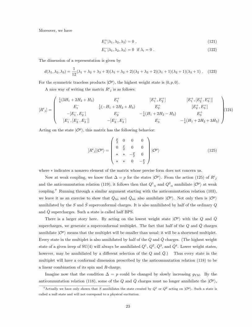
For the symmetric traceless products |Op〉, the highest weight state is |0, p, 0〉.A nice way of writing the matrix Rij is as follows:

[Rij ] =

14 (3H1 + 2H2 +H3) E+

1 [E+1 , E

+2 ] [E+

1 , [E+2 , E

+3 ]]

E−114 (−H1 + 2H2 +H3) E+

2 [E+2 , E

+3 ]

−[E−1 , E−2 ] E−2 − 1

4 (H1 + 2H2 −H3) E+3

[E−1 , [E−2 , E

−3 ]] −[E−2 , E

−3 ] E−3 − 1

4 (H1 + 2H2 + 3H3)

(124)

Acting on the state |Op〉, this matrix has the following behavior:

[Rij ]|Op〉 =

p2 0 0 0

0 p2 0 0

∗ ∗ −p2 0

∗ ∗ 0 −p2

|Op〉 (125)

where ∗ indicates a nonzero element of the matrix whose precise form does not concern us.

Now at weak coupling, we know that ∆ = p for the states |Op〉. From the action (125) of Rij

and the anticommutation relation (119), it follows then that Q1α and Q2

α annihilate |Op〉 at weak

coupling.7 Running through a similar argument starting with the anticommutation relation (103),

we leave it as an exercise to show that Q3α and Q4α also annihilate |Op〉. Not only then is |Op〉annihilated by the S and S superconformal charges. It is also annihilated by half of the ordinary Q

and Q supercharges. Such a state is called half BPS.

There is a larger story here. By acting on the lowest weight state |Op〉 with the Q and Q

supercharges, we generate a superconformal multiplet. The fact that half of the Q and Q charges

annihilate |Op〉 means that the multiplet will be smaller than usual; it will be a shortened multiplet.

Every state in the multiplet is also annihilated by half of the Q and Q charges. (The highest weight

state of a given irrep of SU(4) will always be annihilated Q1, Q2, Q3, and Q4. Lower weight states,

however, may be annihilated by a different selection of the Q and Q.) Thus every state in the

multiplet will have a conformal dimension prescribed by the anticommutation relation (118) to be

a linear combination of its spin and R-charge.

Imagine now that the condition ∆ = p could be changed by slowly increasing gYM. By the

anticommutation relation (118), some of the Q and Q charges must no longer annihilate the |Op〉,7Actually we have only shown that S annihilates the state created by Q1 or Q2 acting on |Op〉. Such a state is

called a null state and will not correpond to a physical excitation.

23

which in turn means that the multiplet must lengthen. States are not created and destroyed by

tuning gYM and so the only way for lengthening to happen is for two short multiplets to combine

together to form a longer one. Sometimes this lengthening does indeed occur. However, a careful

study of the representations of the N = 4 superconformal algebra shows that there is no way for

the multiplet generated by |Op〉 to combine with anything else [13]. Thus the conformal dimensions

of everything in the |Op〉 superconformal multiplet are protected, i.e. independent of gYM.

Consider the example |O2〉 = cIJφIφJ |0〉 which is a set of 20 scalar operators with dimension

∆ = 2. If we act on these states using a single Qi or Qj , the SUSY transformation rule (114) tells us

we get spinors of the schematic form λiφJ and λiφJ both with ∆ = 5/2. Acting again with a single

Qi or Qj , we get a larger variety of possibilities with ∆ = 3. We distinguish the possibilities by their

representation under the Lorentz group. There are complex scalar operators of the schematic form

λiλj + [φI , φJ ]φK , vectors of the form φIDµφJ + λjσ

µλi, and an antisymmetric two form FµνφI .

The vector we recognize as the conserved R-symmetry current. With scaling dimension ∆ = 7/2,

there is a spinor λj [φI , φJ ] and a spin 3/2 object λjDµφI . This spin 3/2 object is the supercurrent.

Finally, with ∆ = 4, we find a complex scalar along with the stress tensor. The complex scalar turns

out to be the Lagrangian density and the theta term εµνρλFµνF ρλ. Given that the stress tensor

and conserved current can be found in the O2 multiplet, it should not be too surprising that the

conformal dimensions here are protected.

We can be more precise about the representations involved. Label a state by its weights under

SU(4) and the Lorentz group SU(2)×SU(2), |λ1, λ2, λ3〉(s1,s2), for example |Op〉 = |0, 2, 0〉(0,0). The

supercharges have the weights

Q1 ∼ [1, 0, 0](± 12 ,0) , Q

2 ∼ [−1, 1, 0](± 12 ,0) , Q

3 ∼ [0,−1, 1](± 12 ,0) , Q

4 ∼ [0, 0,−1](± 12 ,0) , (126)

Q1 ∼ [−1, 0, 0](0,± 12 ) , Q2 ∼ [1,−1, 0](0,± 1

2 ) , Q3 ∼ [0, 1,−1](0,± 12 ) , Q4 ∼ [0, 0, 1](0,± 1

2 ) . (127)

The structure of the O2 multiplet can be summarized pictorially. Each entry in the table gives the

highest weight state of the SU(4)×SU(2)×SU(2) representation. Arrows pointing to the left indicate

the action of Q3 or Q4 while arrows pointing to right indicate Q1 or Q2:

∆

2 |0, 2, 0〉(0,0)

52 |0, 1, 1〉( 1

2 ,0) |1, 1, 0〉(0, 12 )

3

|0,1,0〉(1,0)|0,0,2〉(0,0)

|1, 0, 1〉( 12 ,

12 )

|0,1,0〉(0,1)|2,0,0〉(0,0)

72 |0, 0, 1〉( 1

2 ,0) |1, 0, 0〉(1, 12 ) |0, 0, 1〉( 12 ,1) |1, 0, 0〉(0, 12 )

4 |0, 0, 0〉(0,0) |0, 0, 0〉(1,1) |0, 0, 0〉(0,0)

(128)

From this table and the dimension formula (123), we learn the dimensions of the various SU(4)

24

representations involved. We can write the table in a perhaps more transparent form, replacing

|λ1, λ2, λ3〉(s1,s2) with dim(λ1, λ2, λ3)s1+s2

∆

2 200

52 201/2 201/2

3 61

100151

61

100

72 41/2 43/2 43/2 41/2

4 10 12 10

(129)

In Professor van Nieuwenhuizen’s lectures, we considered the Kaluza-Klein reduction of type IIB

supergravity on AdS5×S5. Let µ, ν index AdS5 and a, b index the S5. Comparing with table III of

[14], we can make the following replacements in our table above

∆

2 haa + aabcd

52 ψ(a) ψ(a)

3 Aµν

Aabhaµ + aµabc

AµνAab

72 λ ψµ ψµ λ

4 B hµν B

(130)

In this table hAB are metric fluctuations, aABCD are fluctuations of the RR four-form potential,

and AAB are fluctuations of a complex combination of the NSNS and RR two-form potentials. The

axio-dilaton is B, the gravitino is ψA, and the dilatino is λ.

In the context of the AdS/CFT correspondence, the complex scalar couples to the boundary

value of the axio-dilaton field in the KK reduction. The stress tensor couples to the boundary value

of the metric. The spin 3/2 field couples to the gravitino. The antisymmetric two-form couples to

fluctuations of the complexifed two-form potential A2 + iB2. The vector field and the scalars in the

20 couple to linear combinations of fluctuations of the RR four-form and the metric. And so on.

Thus concludes a basic check of the correspondence between N = 4 SU(N) SYM and type IIB

string theory on AdS5 × S5.

25

4.2 An Aside on N = 1 theories

There exist many generalizations of the original AdS/CFT correspondence at this point. A number

of them involve four dimensional gauge theories with only N = 1 supersymmetry. There is a much

simpler version of the check that we performed above in this case. Superconformal theories with

N = 1 supersymmetry have a U(1) R-symmetry. The eight supercharges are then conventionally

denoted Qα, Qβ , Sα and Sβ . The supercharges Qα and Qα can be written with the aid of Grassman

variables θ and θ,

Qα =∂

∂θα− iσααmθα∂m , (131)

Qα = − ∂

∂θα+ iθασαα

m∂m . (132)

Conventionally the R-symmetry is normalized such that R(Q) = −1, which then implies R(θ) = 1.

As Q is morally the square-root of Pµ, it must also be true that ∆(Q) = 1/2.

We can write the N = 4 theory in N = 1 notation. There are three chiral superfields conven-

tionally labeled X, Y , and Z, the lowest components of which are x = φ1 + iφ2, y = φ3 + iφ4 and

z = φ5 + iφ6. The charges Q and Q function something like holomorphic and anti-holomorphic

derivatives in this case. Thus X, Y , and Z would be annihilated by Q and also by S and S. Thus

they are the lowest weight states of a shortened superconformal multiplet. Indeed, a symmetrized

product xqyrzp−q−r is already traceless and is an example of the operators of the type Op we

discussed before.

There is an F-term in the action for a N = 1 theory of the form∫d4xd2θW ,

where W is the superpotential. It is clear that for a superconformal theory with unbroken U(1) R-

symmetry and scale invariance, W must have R-charge two and conformal dimension three. InN = 4

SYM, the superpotential is cubic W ∼ trX[Y,Z]. Thus by symmetry one finds that 3RX = 2∆X

and similarly for Y and Z and the operator xqyrzp−q−r. But for free fields, ∆x = 1 and indeed

because Op is protected, ∆(Op) = p. The subsector of operators xqyrzp−q−r are often called chiral

primaries; they always satisfy the relation 2∆ = 3R in four space-time dimensions. Indeed, with

an inner product on the state space, one can prove more generally the so-called BPS inequality

∆ ≥ 3|R|/2 for scalar operators.

5 Trace Anomalies

Recall from last semester that in two dimensional CFTs the trace of the stress tensor need not vanish

on curved manifolds:

〈Tµµ 〉 =c

24πR . (133)

In fact, the condition that this anomaly vanish led us to consider bosonic string theory only in 26

dimensions and superstring theory only in ten. This trace anomaly is in fact a general feature of

26

CFTs in even numbers of space-time dimensions. Given diffeomorphism invariance and hence a

convariantly conserved stress tensor, it is equivalent to the statement that the dilation current xµT νµ

is not conserved.

In four dimension, the structure of the trace anomaly is more complicated. There are several

candidate curvature invariants – RµνρλRµνρλ, RµνRµν , R2 and R – which all have the correct

scaling dimension to sit on the right hand side of the trace anomaly. It is convenient to replace

RµνρλRµνρλ and RµνRµν with the square of the Weyl curvature and the Euler density

I ≡WµνλρWµνλρ = RµνλρRµνλρ − 2RµνRµν +1

3R2 , (134)

E4 ≡1

4δµνρλαβγδR

αβγδRµνρλ = RµνρλRµνρλ − 4RµνRµν +R2 . (135)

We then write the trace anomaly in the (almost) conventional form

〈Tµµ 〉 =1

(4π)2(cI − aE4 + dR+ eR2) . (136)

I say almost because we can set e = 0. The reason is something called Wess-Zumino consistency.

If we imagine that this trace anomaly comes from varying an effective action with respect to scale

transformations gµν → e2σgµν , then like partial derivatives, variations should commute. By assump-

tion, the trace anomaly equation can be derived from the variation δ1W =∫

d4x〈Tµµ 〉δσ1. But then

since [δ1, δ2] = 0 and since the variation δR ∼ σ, it follows that an R2 term is not Wess-Zumino

consistent.

The values of d, c, and a are theory dependent. A one loop calculation is required to determine

them. While d turns out to be sensitive to the regularization scheme chosen, a and c are physical and

can be related to coefficients in the two and three point correlation functions of the stress tensor. For

superconformal theories, a and c are also related to correlation functions of the R-symmetry current

– not perhaps too surprising since we saw above that Jµ and Tµν sit inside the same supermultiplet.

To avoid a one-loop calculation, we look up the results for free fields for example in Chapter 6.3 of

Birrell and Davies [15]. The free fields of interest are a conformally coupled scalar φ, satisfying the

equation ( +R/6)φ = 0 in d = 4, a massless Weyl fermion λ, and a gauge field Aµ.

180(a− c) 360c degeneracy

φ −1 1 6N2

λ − 74

112 4N2

Aµ 13 62 N2

total 0 90N2

(137)

We have also included in this table the degeneracy of these fields in N = 4 SU(N) SYM in the large

N limit. We may then conclude that at weak coupling in the large N limit

a = c =N2

4. (138)

Thus for N = 4 SU(N) SYM in the large N limit, the trace anomaly takes the somewhat simpler

27

form

〈Tµµ 〉 =N2

32π2

(RµνRµν −

1

3R2

). (139)

These anomaly coefficients cannot depend on marginal operators in a CFT, and so they remain

the same for all values of g2YMN . Thus if we compute the trace anomaly using AdS/CFT, we should

get the same answer. Let us check.8 From the result for the bare holographic stress tensor (76) and

the counter-terms (77), we can read off the renormalized stress tensor:

−√−g0T

µν = lim

z→0

√−γκ2

[Kµν −Kγµν +

3

Lγµν +

1

4LRγµν −

1

2Rµν]. (140)

The calligraphic font is used to remind us to use the boundary metric γµν (defined in (64)) in

constructing these curvature invariants. In what follows, it is more convenient to work directly with

the field theory metric gµν , defined in (65). Because Rµν is invariant under global rescaling of the

metric, we have that Rµν = Rµν , where Rµν is constructed from gµν . We also have that R = z2

L2 R.

Note that we could have added further finite counter-terms of the form O(R2) to the boundary

gravity action. This type of ambiguity parallels the scheme dependent possibility of having a R in

the trace of the stress tensor. A R in the trace can come from varying a R2 counter-term in the

effective action.

Given the holographic stress-tensor (140), it is then straightforward to take a trace:

−√−g0T

µµ = lim

z→0

√−γκ2

[−3K +

12

L+

1

2LR]. (141)

We unpack this trace result using the boundary expansion of the metric (66) in the particular case

d = 4. Analogous to the scalar case, boundary conditions allow us to set g(0)µν and g

(4)µν . The other

coefficients in the expansion are fixed in terms of these two coefficients by Einstein’s equations. We

will need the following relations in what follows.

Claim One:

RL =z2

L

[−6 tr g−1

(0)g(2) + 2z2 tr(g−1(0)g(2)g

−1(0)g(2)) + z2(tr g−1

(0)g(2))2 + . . .

], (142)

Claim Two:

RµνRµν − 1

3R2 = 4

(tr g−1

(0)g(2)g−1(0)g(2) − (tr g−1

(0)g(2))2)

+O(z2) , (143)

The curvature Rµν is computed with the metric gµν . Note that Rµν |z=0 = R[g(0)µν ].

Claim Three:

tr g−1(0)g(4) =

1

4tr(g−1

(0)g(2)g−1(0)g(2)) , (144)

Claim Four:

tr g−1(0)h(4) = 0 . (145)

8This check was first performed in another early AdS/CFT paper [16].

28

We will derive these four relations later.

We analyze each of the three terms in the trace (141) separately. Note first that we have

√−γ =

L4

z4

√−g . (146)

Given that an outward pointing normal is n = (0,−z/L), the trace of the extrinsic curvature is

K =z5

L5

1√−g

∂zL5

z5

√−g(− zL

)= − 1

Lz5 1√−g

∂z

√−gz4

. (147)

The square root of the determinant√−g expands then as

√−g =

√−g(0)

[1 +

z2

2tr g−1

(0)g(2) +z4

2tr g−1

(0)g(4) −z4

4tr g−1

(0)g(2)g−1(0)g(2) +

+z4

8(tr g−1

(0)g(2))2 +

z4

2log z tr g−1

(0)h(4) + . . .]. (148)

We’re making use of the familiar fact that det g = exp tr log g and the Taylor series expansion√

1 + x = 1 + x2 −

x2

8 + . . ..

The first term in the trace is

−3√−γKκ2

=3L3

κ2z∂z

1

z4

√−g , (149)

=3L3

κ2

√−g(0)z∂z

[1

z4+

1

2z2tr g−1

(0)g(2) +1

2log z tr g−1

(0)h(4) + . . .

]=

3L3

κ2

[− 4

z4− 1

z2tr g−1

(0)g(2) +O(z2)

]√−g(0) .

To go from the second to the third line, we used Claim Four. The second term in the trace is√−γκ2

12

L=

12L3

κ2

√−g(0)

[ 1

z4+

1

2z2tr g−1

(0)g(2) +1

2tr g−1

(0)g(4) −1

4tr g−1

(0)g(2)g−1(0)g(2) +

+1

8(tr g−1

(0)g(2))2 +

1

2log z tr g−1

(0)h(4) + . . .]. (150)

Notice that the log term will again vanish by Claim Four. The third term is√−γκ2

RL2

=1

2κ2

L5

z4

√−g(0)

[1 +

z2

2tr g−1

(0)g(2) + . . .

]z2

L2

×[−6 tr g−1

(0)g(2) + 2z2 tr(g−1(0)g(2)g

−1(0)g(2)) + z2(tr g−1

(0)g(2))2 + . . .

], (151)

where we have used Claim One. Assembling the three pieces, we get

−〈Tµµ 〉 =L3

κ2

[−12 + 12

z4+−3 + 6− 3

z2tr g−1

(0)g(2) + 6 tr g−1(0)g(4) + (−3 + 1) tr g−1

(0)g(2)g−1(0)g(2)

+

(3

2+

1

2− 3

2

)(tr g−1

(0)g(2))2 +O(z2)

]=

L3

κ2

[6 tr g−1

(0)g(4) − 2 tr g−1(0)g(2)g

−1(0)g(2) +

1

2(tr g−1

(0)g(2))2

]=

L3

2κ2

[− tr g−1

(0)g(2)g−1(0)g(2) + (tr g−1

(0)g(2))2]

=L3

2κ2

1

4

[−RµνRµν +

1

3R2

]∣∣∣∣z=0

. (152)

29

In the first line, we see how crucial the counter-terms (77) are for getting a finite result. In some

sense, we can view the first line as a derivation of the coefficients in the counter-term action (77).

To go from the second to the third equality, we use Claim Three. To go from the third to the fourth

equality, we use Claim Two.

The gravity computation (152) is then consistent with the field theory one (139) provided we

make the identification

L3

8κ2=

N2

32π2. (153)

Does this identification make sense? We can read off the ten dimensional gravitational coupling

constant from the SUGRA action (8):

1

2κ210

=1

(2π)7`8sg2s

. (154)

By usual KK reasoning, the five dimensional coupling should then be

1

2κ2=

Vol(S5)L5

2κ210

=Vol(S5)L5

(2π)7`8sg2s

=Vol(S5)

(2π)7(4πgsN)2 1

L3

1

g2s

.

where in the third line, we used that (L/`s)4 = 4πgsN . Using also that Vol(S5) = π3, we find indeed

the relation (153).

That there be some relation between a and c for theories with Einstein gravity duals is a foregone

conclusion. There is only one parameter these coefficients can depend on, L3/κ2. That relation we

have seen is a = c.

Justifying the Claims

The proof of the claims requires writing down the Einstein Equations ,

RAB = − d

L2GAB , (155)

in a gauge fixed background where Gµz = 0. The Christoffel symbols are

Γzzz = −1

z, Γzµz = Γµzz = 0 , (156)

Γzµν = −1

2gµν,z +

1

zgµν , (157)

Γµzν =1

2gµλgνλ,z −

1

zδµν , (158)

Γµνλ = γµνλ (159)

where γµνλ are the Christoffel symbols for the metric gµν along a constant z-slice. The Ricci curvature

takes the usual form

RAB = RCACB = −ΓCAC,B + ΓCAB,C − ΓEACΓCEB + ΓEABΓCEC . (160)

30

The zz-component of the Ricci curvature is then

Rzz = −1

2tr g−1

(g′′ − 1

zg′)

+1

4tr g−1g′g−1g′ − d

z2. (161)

Specializing to d = 4, the zz-component of Einstein’s equations Rzz = − dL2Gzz then leads directly

to claims three and four. For the remaining claims, we also need the other components of the Ricci

curvature:

Rµz =1

2gµλ(∇νg′λµ −∇λg′µν) , (162)

Rµν = Rµν −1

2g′′µν +

d− 1

2zg′µν −

(1

4g′ − 1

2zg

)µν

tr g−1g′

+1

2(g′g−1g′)µν −

d

z2gµν . (163)

Note that Rµν is computed with gµν , or since Rµν is invariant under global scale transformations,

equivalently with γµν . Thus we could also call it Rµν .

Claim two follows from the first order terms in a small z expansion of Rµν = − dL2Gµν :

Rµν + 2g(2)µν + g(0)

µν tr g−1(0)g(2) + . . . = 0 . (164)

From this expression, we can read off both Rµν and its trace:

Rµν = −2g(2)µν − g(0)

µν tr g−1(0)g(2) , (165)

R = −6 tr g−1(0)g(2) . (166)

From these two expressions, claim two follows after a short computation. Note that the result for R

is the leading order term in Claim One. To compute the subleading terms, we need to look at the

subleading terms in the µν trace of Einstein’s equations:

0 = R− 1

2tr g−1g′′ +

2d− 1

2ztr g−1g′ − 1

4(tr g−1g′)2 +

1

2tr g−1g′g−1g′ , (167)

from which we find that

R(2) −1

2· 12 tr g−1

(0)g(4) +1

2· 2 tr g−1

(0)g(2)g−1(0)g(2)

+7

2· 4 tr g−1

(0)g(4) −7

2· 2 tr g−1

(0)g(2)g−1(0)g(2)

−1

4· 22(tr g−1

(0)g(2))2 +

1

2· 22 tr g−1

(0)g(2)g−1(0)g(2) = 0 . (168)

We’ve not collected terms so that the reader can more easily follow the algebra. Collecting terms

now yields

0 = R(2) + 8 tr g−1(0)g(4) − 4 tr g−1

(0)g(2)g−1(0)g(2) − (tr g−1

(0)g(2))2 . (169)

By claim three, this result then immediately yields the subleading terms in Claim One.

31

The Two Dimensional Case

To fix the normalization of Newton’s constant in terms of the central charge c, let us also review the

two dimensional computation. The two dimensional stress tensor follows as a special case from (76)

and (77):

−√−g0T

µν = lim

z→0

√−γκ2

[Kµν −Kγµν +

1

Lγµν

]. (170)

Taking the trace then straightforwardly yields

−√−g0T

µµ = lim

z→0

√−γκ2

[−K +

2

L

]. (171)

We follows the same steps as we did in the four dimensional case, computing small z expansions of

K and√−γ:

K =z3

L3

1√−g

∂zL3

z3

√−g(− zL

)= − 1

Lz3 1√−g

∂z

√−gz2

, (172)

√−g =

√−g(0)

[1 +

z2

2tr g−1

(0)g(2) +z2

2log z tr g−1

(0)h(2) + . . .]. (173)

The first term in (171) is then

−√−γKκ2

=L

κ2z∂z

1

z2

√−g , (174)

=L

κ2

√−g(0)

[− 2

z2+

1

2tr g−1

(0)h(2) +O(z2)

],

while the second is√−γκ2

2

L=

2L

κ2

√−g(0)

[ 1

z2+

1

2tr g−1

(0)g(2) +1

2log z tr g−1

(0)h(2) + . . .]. (175)

Putting the two pieces together yields

−Tµµ =L

κ2tr g−1

(0)g(2) , (176)

where we have used that tr g−1(0)h(2) = 0, something that follows from a small z expansion of the µν

components of Einstein’s equations (see (163)). We now need to relate this expression to the Ricci

scalar R computed from gµν . The trace of the µν components of Einstein’s equations (167) now

gives

R = −2 tr g−1(0)g(2) + . . . . (177)

Inserting this expression into (176) yields

Tµµ =L

2κ2R , (178)

which agrees with the field theory result (133) provided we make the identification

L

2κ2=

c

24π. (179)

32

6 Hawking-Page Phase Transition

[These notes are loosely based on Witten’s paper [17] which appeared only a month after his seminal

paper on AdS/CFT [3].]

In 1983, working purely from gravity considerations, Hawking and Page [18] argued that AdS

in global coordinates, when the temperature is raised above a critical value Tc, undergoes a first

order phase transition to a space-time containing a black hole. Given our knowledge of the AdS/CFT

correspondence, there must be some interesting dual interpretation of this phase transition for N = 4

SYM on S3 × S1.

Let the radius of S3 be b and the circumference of the S1, which is also the inverse temperature,

be β. Because of the Rφ2 coupling, the conformal scalars in N = 4 SYM will all get masses

proportional to 1/b. There are no zero modes for the fermions or gauge field on the S3; like for

the scalar, the minimum energy modes are proportional to 1/b. Thus at zero temperature, N = 4

SYM becomes trivial. There are no excitations. But for temperatures large compared to the inverse

radius of the S3, β < b, one anticipates something interesting might happen as the low energy modes

become thermally populated. Indeed, in the zero coupling limit, one finds a Hagedorn type transition

in a large N limit [Bo Sundborg, hep-th/9908001]. In view of the AdS/CFT correspondence, the

Hawking and Page result implies there is also a phase transition in the large N , large g2YMN limit.

Presumably, the phase transition exists for all g2YMN although its precise nature is not known.

N.B.: Because we are at finite volume, one would naively expect no non-analyticities in the free

energy as a function of T . We get a phase transition precisely because we have taken a large N

limit.

Let us review the Hawking-Page calculation using AdS/CFT machinery. We begin with the

metric ansatz

ds2

L2=

1

z2

(−f(z)dt2 + b2dΩ2

3 +dz2

f(z)

). (180)

Einstein’s equations are RAB = −4GAB/L2. The θ1θ1 component in a parametrization of the S3

where

dΩ23 = dθ2

1 + sin2 θ1dθ22 + sin2 θ1 sin2 θ2dφ

2 ,

implies

f ′ − 4

zf +

2z

b2+

4

z= 0 .

The most general solution for f is then

f(z) = 1 +z2

b2+ cz4 . (181)

(One may check that the remaining Einstein equations are also satisfied.) AdS in global coordinates

is recovered by setting c = 0. The conformal boundary is located at z = 0 and we keep only the

region z > 0. (We can recover the Poincare patch by further sending b → ∞ and rescaling the

S3 coordinates to “zoom in” on a small region of the sphere.) We may also introduce a black hole

33

horizon with a nonzero value of c. The horizon is located at gtt(z = zh) = 0, which then implies

c = −1 + z2h/b

2

z4h

. (182)

We now use the usual trick of extracting the Hawking temperature by insisting that the Euclidean

metric be regular at z = zh. The relevant pieces of the Euclidean line element are

ds2E =

L2

z2h

(f ′(zh)(z − zh)dτ2 +

dz2

f ′(zh)(z − zh)+ . . .

), (183)

where we have only kept the leading terms in an expansion of the line element near z = zh. We

introduce a new radial variable r such that

L2dz2

z2hf′(zh)(z − zh)

= dr2 ⇒ r =2L

zh√|f ′(zh)|

√zh − z . (184)

(Note we have to be a little careful with signs since f ′(zh) < 0 and z < zh.) The Euclidean metric

can now be written in terms of r:

ds2E =

L2

z2h

|f ′(zh)|r2 z2h|f ′(zh)|

4L2dτ2 + dr2 + . . .

=f ′(zh)2

4r2dτ2 + dr2 + . . .

We now introduce an angular variable θ such that

|f ′(zh)|dτ2

= dθ , (185)

and where θ has period 2π. Thus, identifying the Hawking temperature TH with one over the

periodicity of τ , we find

TH =|f ′(zh)|

4π

=

∣∣∣ 2zhb2 − 1+z2h/b2

z4h4z3h

∣∣∣4π

=4zh

+ 2zhb2

4π. (186)

This result for the temperature shows that for a given value of TH , there are generically either no

or two corresponding values of zh. See figure 2. The larger value of zh corresponds to a small black

hole because the horizon is further from the boundary and has a smaller area. The smaller value of

zh corresponds to a large black hole. The small black holes are similar to black holes in flat space

while we will see in a moment that the large black holes actually have positive specific heat.

To compute which phase is stable, AdS in global coordinates or the black hole, we need to

compute a free energy. AdS/CFT tells us that the free energy can be computed from the log of the

CFT partition function:

F = −T logZ = −T log eSE = TSE (187)

34

small black holeslarge black holes

( 2 , 2 Π

0 1 2 3 4 50.0

0.2

0.4

0.6

0.8

1.0

1.2

zh

b

b TH

Figure 2: Temperature as a function of horizon location.

where we use our usual formula for the regulated gravity action

Sgrav = SEH + SGH + Sctr , (188)

and we set T = TH . (I believe the only real difference here for us between SE and Sgrav is that for

SE , we integrate over a circle rather than over all time.)

First the Einstein-Hilbert term:

SEH = − 1

2κ2

∫d5x√−G

(R+

12

L2

)= − L3

2κ2Vol(S3)

1

T

∫ zh

ε

dz

(−8

z5

)b3

= −L3

κ2Vol(S3)

1

T

(−1

z4h

+1

ε4

)b3 .

In the second line, we used that R = −20/L2.

Next the Gibbons-Hawking term:

SGH = − 1

κ2

∫d4x√−γK

Note that

K =1√−G

∂z√−G

(−zLf1/2

)= −z5∂z

(f1/2

z4

1

L

).

35

We then find

SGH =L3

κ2b3 Vol(S3)

1

T

(zf1/2∂z

(f1/2

z4

))∣∣∣∣z=ε

= −L3

κ2b3 Vol(S3)

1

T

(4

ε4+

3

b2ε2− 2(1 + z2

h/b2)

z4h

+ . . .

)Third, the counter term:

Sctr =1

κ2

∫d4x√−γ(

3

L+L

4R)

=L3

κ2b3 Vol(S3)

1

T

1

z4f1/2

(3 +

3

2

z2

b2

)∣∣∣∣z=ε

=L3

κ2b3 Vol(S3)

1

T

(3

ε4+

3

b2ε2+

3

8

(1

b4− 4

z4h

− 4

b2z2h

)+ . . .

)The divergent 1/ε4 and 1/ε2 terms vanish leaving the result

Sgrav =L3

κ2Vol(S3)b3

1

T

[3

8b4− 1

2z4h

+1

2b2z2h

]. (189)

This result has an amazing amount of physics that we can now extract. From this on-shell action,

we deduce the free energy of the black hole and thermal AdS phases:

Fbh =L3

κ2Vol(S3)b3

[3

8b4− 1

2z4h

+1

2b2z2h

], (190)

FAdS =L3

κ2Vol(S3)b3

3

8b4. (191)

• The FAdS is essentially a Casimir energy and can be deduced from the conformal anomaly a.

(See for example my paper with Kuo-Wei Huang [19].) In more detail, we assume that the

pressure is independent of the volume. Given that P = −(∂F/∂V )T , it follows that F = −PV .

This same pressure appears in the diagonal spatial entries of the stress tensor at equilibrium.

By a Schwarzian type derivative transformation, the pressure can be related to the conformal

anomaly a.

• Consider the free energy difference

∆F = Fbh − FAdS =L3

2κ2b3 Vol(S3)

1

z4h

[z2h

b2− 1

](192)

In other words, the black hole is favored when zh < b and thermal AdS is favored when zh > b.

• Because zh <√

2zh, we see that the large black holes become favored at high temperature.

The small black holes – the ones that are similar to Schwarzschild black holes in flat space

– are thermodynamically unstable. Given that we know Schwarzschild black holes become

hotter the smaller they get, i.e. they have negative heat capacity, that the small black holes

are not thermodynamically favored should not be that surprising.

• For fun, we can consider the b → ∞ limit where the S3 is replaced by R3. In this case, we

should divide by the volume factor and consider the energy density instead:

fbh ≡Fbh

Vol(S3)b3= − L3

2κ2(πT )4 , (193)

36

-

-

-

-

Δ

Figure 3: Free energy difference as a function of temperature.

where we have used the fact that T = 1/πzh in the limit b → ∞. Using the fact that

π2L3/κ2 = N2/4 that we used in computing the conformal anomaly a holographically, we find

that

fbh = −π2

8N2T 4 .

For free N = 4 SYM, one can compute the free energy density ffree. (See for example the

paper by Gubser, Klebanov, and Tseytlin [20].) One finds that the strong interactions reduce

the effective number of degrees of freedom.

fbh =3

4ffree .

Much has been made of this factor of 3/4 in the literature. It is at last an interesting prediction

for N = 4 SYM in the strong coupling limit. Lattice calculations involving pure YM produce

similar looking factors relating f at temperatures slightly above confinement to perturbative

calculations in the ultra-high T limit.

• To end this lecture, we can verify the thermodynamic relation between free energy and entropy:

Sbh = −dFbh

dT= −dFbh

dzh

(dT

dzh

)−1

= −L3

κ2Vol(S3)b3

(2

z5h

− 1

b2z3h

)4π

(− 4

z2h

+2

b2

)−1

=L3

κ2Vol(S3)b3

4π

z3h

=A

4GN, (194)

37

where A is the area of the event horizon and GN is Newton’s constant. [Conventionally

12κ2 = 1

16πGN.] One could consider this short calculation a sort of holographic derivation of

black hole entropy.

7 Current-Current Correlation Functions and Conductivity

Let us start by discussing current-current correlation functions in field theory more generally. In

the vacuum state of a conformal field theory, current conservation and scale invariance together

constrain the two-point function to take the form

〈Jµ(x)Jν(0)〉 =c

x2(d−1)

(δµν − 2

xµxν

x2

). (195)

We work in Euclidean signature, at least to start, to keep the discussion a bit simpler. In vacuum,

then, the correlation function is determined by symmetry and the choice of an overall constant c. If

we now consider the Fourier transform

Gµν(k) =

∫ddx eikx〈Jµ(x)Jν(0)〉 , (196)

the result is in general UV divergent, requiring some type of regularization. The Fourier transformed

Green’s function can be written as

Gµν(k) = c

(δµνI−1(k) + 2

∂2

∂kµ∂kνI0(k)

), (197)

where we have defined

In(k) ≡∫

ddxeikx

x2(d+n)= kd+2n(2π)d/2

∫ ∞kε

J d2−1(kx)

(kx)3d2 +2n

d(kx) . (198)

We regulated the Fourier transform by introducing a small distance cut-off ε. The radial integral

evaluates to ∫ ∞kε

J d2−1(kx)

(kx)3d2 +2n

d(kx) =Γ(−n− d

2

)2d/2

(1

2d+2nΓ(d+ n)− 1

(kε)d+2n

). (199)

The final expression for the Fourier transform of the current-current correlation function is then

Gµν(k) = cπd/2Γ

(2− d

2

)2d−3Γ(d)

kd−2

(δµν − kµkν

k2

)+O(ε2−d) . (200)

The UV divergent term of order ε2−d is k-independent and violates the Ward identity, so we throw

it away. In even dimensions, the divergence in Γ(2 − d/2) can be swapped for a logarithmic term

log(kε). If we think of the Green’s function as a way of propagating a disturbance away from a

localized source, an important point here is that even powers of k can be replaced in position space

by derivatives acting on a Dirac delta function. They thus affect the behavior of the system locally

at the source and do not affect the long distance behavior. From this point of view, it is clear that

in even dimensions, a Green’s function proportional to kd−2 must be supplemented by a log to give

the requisite non-analyticity.

38

Knowing what to expect we now switch back to AdS/CFT and the action (55) in the specific

case of AdS5. Consider a small, transverse, plane wave fluctuation of the gauge field

A1 = a(z)eiqx2

+ c.c. (201)

The equation of motion for the gauge field constrains a(z) to obey the second order differential

equation

(z−1a′

)′=q2

za , (202)

where ′ denotes ∂z. The small z expansion (58) has the specific form

a = a0

(1 +

q2

2z2 log z − 3

64q4z4 +

q4

16z4 log z + . . .

)+ a2z

2

(1 +

q2

8z2 + . . .

)+ c.c. , (203)

where now because the two series overlap, logarithms have appeared.

In varying the action, we find the boundary term

δS =1

e2

∫z=ε

d4xL

zδA1∂zA1 . (204)

Plugging in the series expansion, we find that

δS =L

e2

∫z=ε

d4x δa∗0

(2a2 +

q2

2a0 + q2a0 log z

)+ c.c. (205)

The one point function of the current is thus proportional to the term in parentheses:

〈J1〉 =L

e2

(2a2 +

q2

2a0 + q2a0 log(qε)

)eiqx

2

+ c.c. (206)

The log independent term proportional to q2a0 is ambiguous and can be shifted away by an appro-

priate choice of cut-off inside the argument of the log. We thus find the result (63) we had before,

that the one-point function of the current is proportional to the coefficient of the zd−2 term in the

expansion of Aµ. Naively, the a2 term seems to be ambiguous as well. While the real part of a2

is indeed rather meaningless, an imaginary part cannot be shifted away and has implications for

dissipative behavior in the field theory.

The pure AdS geometry is simple enough that the differential equation (202) has an analytic

solution. Picking the solution that exponentially damps out in the interior, we find

a = a0qzK1(qz) = a0

(1 +

q2z2

4(2γ − 1 + 2 log

qz

2)

)+ . . . . (207)

Referring to the expression for the one-point function of the current (206), we can extract the

Fourier transform of the two-point current correlation function by varying the one-point function

with respect to the external gauge field:

G11(k) =δ〈J1〉δa0

∼ q2 log qε . (208)

This q2 log qε scaling is precisely what we expect from our earlier field theory discussion and the

general result (200).

39

Conductivity

If we consider a more general state with less symmetry, the current correlation functions become less

constrained and more interesting. Consider the case of d = 3 and nonzero temperature, for which

there exists a black brane metric with line element

ds2 =L2

z2

(−f(z)dt2 +

dz2

f(z)+ dx2 + dy2

), (209)

where f(z) = 1 − z3

z3h. The horizon is at z = zh, while the boundary as usual is at z = 0. The

Hawking temperature of this black brane is T = 1/πzh, as one can for example check by looking at

the periodicity of the Euclidean time tE = it.

On the field theory side, a nonzero temperature produces a plasma and a preferred rest frame.

One can write two tensor structures that are compatible with the remaining symmetries and the

Ward identity kµGµνR (k) = 0:

GµνR (k) = ikd−2(P (1)µν K

(1)(ω,k) + P (2)µν K

(2)(ω,k)) (210)

where

P(1)00 = P

(1)0i = P

(1)i0 = 0 , P

(1)ij = δij −

kikjk2

, P (2)µν = ηµν −

kµkνk2

. (211)

The functions K(1) and K(2) can only depend on the wave vector k through the dimensionless ratios

ω/T and |k|/T . In the limit T → 0, we must recover the vacuum result K(1) = 0 and K(2) = c.

It turns out that in the limit k → 0, K(1) also vanishes while K(2) will in general be a nontrivial

function of ω/T .

To use AdS/CFT to compute these correlation functions in the limit k → 0, consider a small

perturbation

Ax = a(z)e−iωt . (212)

Such a gauge field corresponds to an external electric field of strength Ex = −∂tAx|z=0 = iωa(0)e−iωt

and a current Jx = 1e2 a′(0)e−iωt. The equation of motion is remarkably simple in d = 3,

f(z)∂z(f(z)∂za) = −ω2a . (213)

We solve this equation by defining a new variable ζ such that ∂ζ = f(z)∂z, leading to plane wave

solutions

a = c+eiωζ + c−e

−iωζ . (214)

Note that as ζ → ∞, z → zh, and thus the + solution, which we will keep, corresponds to a plane

wave moving into the horizon. The small z expansion for a(z) is

a(z) = c+(1 + iωz + . . .) , (215)

40

leading us to identify K(2)(ω, 0) = 1e2 . There is a more physical way to think about these response

functions. We’ve computed a current Jx and an external electric field Ex. Through Ohm’s Law,

their ratio should be a conductivity:

σ =Jx

Ex=

1

e2

a′(0)

(iω)a(0)=

1

e2. (216)

Thus, K(2)(ω, 0) is also the optical conductivity. In this holographic example, remarkably it is

independent of temperature. This independence can be traced to a classical electromagnetic duality

of the action for an abelian gauge field in four dimensions (55) [21]. The paper [21] which calculated

the conductivity of this d = 3 holographic plasma, sometimes called the ABJM plasma, has some

historical significance. It is one of the first, if not the first, application of AdS/CFT to condensed

matter systems.

To see the relevance of electromagnetic duality, let us write the optical conductivity in terms of

the boundary values of the electric and magnetic fields:

σ =1

e2

By(0)

Ex(0). (217)

But we should also be able to measure the same conductivity in the dual theory where the electric

and magnetic fields are swapped. As the theory is free, we can leave e untouched; we do not need

to send e→ 1/e. As the fields obey exactly the same equations in the dual theory, the only way for

this independence to occur is if the boundary values are equal.

8 Viscosity

In 2001, Policastro, Son, and Starinets [22] computed the viscosity η of SYM in the large N , large

g2YMN limit using gauge/gravity duality. Their answer, compactly expressed in terms of the entropy

density s, was that

η

s=

~4πkB

. (218)

(We set ~ = kB = 1 in what follows.) This answer has turned out to be remarkable in a number of

respects that are worthy of comment.

• The ratio is remarkably small. Common substances such as air and water have ratios which

depend on temperature and pressure but are at least several dozen times higher. The smallness

of the ratio should be viewed as an effect of strong coupling. Viscosity is proportional to

the rate of momentum diffusion. In strongly coupled systems, many scattering events and a

corresponding substantial amount of time is required for momentum to diffuse over distances

large compared to the mean free path.

• This ratio was later shown to be a universal for any QFT in a rotationally symmetric state

holographically dual to Einstein gravity [23, 24, 25].9

9For anisotropic systems, the viscosity becomes a tensor, introducing a nonuniversal aspect to the story. For the

41

• With current techniques, it is extremely difficult to compute the viscosity for strongly coupled

systems by any other means. For instance, to compute the viscosity numerically using lattice

gauge theory, one must either define the gauge theory in real time and overcome the sign

problem or analytically continue a numerically determined Euclidean Green’s function (see for

example [27]).

• The idea of measuring viscosity in terms of entropy density has found experimental application.

Two experimental hydrodynamic systems which seem to have viscosities that approach the

value (218) from above are the quark-gluon plasma formed in the collision of heavy nuclei [28]

and “fermions at unitarity”, i.e. clouds of fermionic atoms tuned to a strong coupling limit

using a magnetic field and Feshbach resonance [29].

The smallness of the ratio and its universality led Kovtun, Son, and Starinets [23] to conjecture

that the value (218) might actually be a lower bound. From a theoretical point of view, the possibility

of arbitrary sign corrections to 1/4π from higher curvature terms in the dual gravity action has

greatly weakened the case that the lower bound is 1/4π [30, 31, 32]. In fact, there exist certain

gauge/gravity duality constructions where the 1/N corrections are under control and where the

bound is violated by 1/N effects [32]. The fact that there are as yet no experimental counter-

examples and the uncertainty principle argument put forth in the original paper [23] keep hope alive

that there may indeed be a bound although perhaps with a somehwat lower value.

Our first task is to define precisely what we mean by viscosity for SYM. At T > 0, SYM is a

neutral relativistic plasma. At scales smaller than the system size but larger than the mean free path,

which by conformal invariance must be proportional to 1/T , we expect that the plasma admits a

hydrodynamic description. (A good reference here is chapter 15 of [33].) At these scales, the system

is close to thermal equilibrium and can be well described by the variation of conserved quantities,

in this case energy and momentum. Locally, the statement of energy and momentum conservation

is that

∇µTµν = 0 . (219)

Given that Tµν is slowly varying, compared to the scale set by the temperature T , we can expand

Tµν in gradients. At zeroth order in a local rest frame, the stress tensor is diagonal:

Tµν =

ε 0 0 0

0 p 0 0

0 0 p 0

0 0 0 p

, (220)

where ε and p are the energy density and pressure respectively. With knowledge of the equation of

state, we can think of the system as existing at local thermal equilibrium and express ε(T ) and p(T )

as functions of a slowly varying temperature T (x).

p-wave holographic superfluid, which is dual to Einstein gravity, the different components of η have different values

in the ordered phase [26].

42

Hydrodynamics should also describe energy and momentum flow. To that end we introduce a

slowly varying velocity field uµ such that u2 = −1 and for the fluid at rest uµ = (1,~0). At zeroth

order in gradients, the only possible structure for the stress tensor is

Tµν = αuµuν + βgµν . (221)

Comparing with the fluid at rest, one finds that α = ε+p and β = p. Given the equation of state and

the constraint on uµ, the conservation conditions are four evolution equations for the four unknowns

T and ~u.

Next, we consider first order gradient corrections,

Tµν = (ε+ p)uµuν + pgµν − σµν . (222)

To constrain the form of σµν , we fix a point x and frame ~u(x) = 0. We then define T and ~u such

that σ0µ = 0. As properties of the system at thermal equilibrium, T and ~u are only well defined

up to gradient corrections anyway. By rotational symmetry, at the point x, the gradient corrections

must take the form

σij = η

(∂iuj + ∂jui −

2

3δij∂ku

k

)− ζδij∂kuk . (223)

The coefficient η is conventionally called shear viscosity while ζ is the bulk viscosity. In our indexing

conventions, µ and ν include the time direction while i and j do not. The tensor structures ∂iuj

and δij∂kuk have been divided up such that the structure multiplying η is traceless. For conformal

field theories, among which SYM is an example, the trace of the stress tensor must vanish.10 Thus,

the bulk viscosity is zero in our case.

By general covariance, we can write this tensor structure for a general metric and point x:

σµν = ηPµλP νρ(∇λuρ +∇ρuλ −

2

3gλρ∇ · u

), (224)

where we have defined the projector Pµν ≡ gµν +uµuν onto directions orthogonal to uµ. (Note that

curvature corrections involve second derivatives of the metric and would appear at higher order in

our gradient expansion of Tµν .)

In holography, we will extract the viscosity by varying the CFT metric. Let us see how that

works first purely from the CFT side. Consider a metric fluctuation of the form

gij(t, ~x) = δij + hij(t) , (225)

10There could be a trace anomaly, but the trace anomaly is proportional to the curvature and thus higher order in

our gradient expansion.

43

where hii = 0, g00 = −1, and g0i = 0. Let us also take a static situation where uµ = (1,~0). In this

case, we find that

∇xuy = ∂xuy − Γµxyuµ

= Γ0xy

=1

2g00(−∂thxy)

=1

2∂thxy .

Along with the fact that ∇·u = ∂t log√−g = 0 by tracelessness of the metric fluctuation, we obtain

σxy = η∂thxy . (226)

On the gravity side, I will begin with a non-trivial assertion about the form of the CFT stress

tensor, defined on a constant z = z0 hypersurface in the limit z0 → 0 [12]:

Tµν = − limz0→0

√−γ

8πGN

[Kµν −Kδµν +

3

Lδµν +

RL4δµν −

1

2Rµν], (227)

where γµν is the induced metric on the z = ε slice of the geometry, and we have defined the extrinsic

curvature KAB = ∇(AnB) and its trace K = Kµµ in terms of a unit normal vector nA to the

constant z = z0 hypersurface. The Ricci curvature Rµν and scalar R are defined on the same z = z0

hypersurface. In our indexing conventions, A and B include the radial direction u while µ and ν do

not.

The terms in Tµν that depend on Kµν follow from (??) and a variation of the on-shell gravity

action with respect to the boundary metric δSgrav/δgµν .11 As is well known, for classical gravity

theories defined on spacetimes with boundary, in order to have a well defined variational principle, the

usual Einstein action must be supplemented by the Gibbons-Hawking term. The same calculation

that demonstrates the necessity of the Gibbons-Hawking term will produce the Kµν dependent terms

in the CFT stress tensor. The last three terms in (227) are counterterms required to cancel off UV

divergences in δSgrav/δgµν . The counterterms are uniquely determined by requiring them to be

local, covariant, and of smallest engineering dimension. A careful treatment of these counterterms

is often referred to as holographic renormalization. See ref. [8] for a more in depth discussion.

Given the stress tensor (227), our strategy will be to vary the boundary metric in the same

way as we did before using hydrodynamics and isolate the term in (227) that is proportional to the

viscosity. One big difference from what we did before is that gravity will specify the value of η.

Consider the line element

ds2

L2=

1

z2

(−f(z)dt2 + d~x2 +

dz2

f(z)

)+ 2gxy

dx dy

z2, (228)

11There are some subtleties about gauge fixing that I am busy sweeping under the rug. It is usually most straight-

forward to work in a gauge where gAz = 0, in which case varying with respect to gµν is unambiguous. In general, we

should (and can) be more careful.

44

where f(z) = 1 − (z/zh)4 and gxy = e−iωtφ(z). We insist that φ(z) 1 and look at the first

order term in φ(z) in Einstein’s equations RAB = −4gAB/L2. Remarkably, at first order Einstein’s

equations impose the condition that

gxy = 0 , (229)

where the Laplacian is defined using the unperturbed metric. In other words, gxy behaves like a

massless scalar in AdS. There is a theorem about the low energy absorption cross section for massless

scalars in black hole spacetimes which can be used to explain why 1/4π is a universal value for η/s

for QFTs dual to Einstein gravity [23].

Putting universal considerations aside, let us solve gxy = 0 in the hydrodynamic limit ω T .

First we set boundary conditions at the horizon. Assuming that φ ∼ (z− zh)α when z ≈ zh, we find

that α = ±iωzh/4. We want causal boundary conditions, which correspond to waves traveling into

the black brane. This causality constraint means we must choose the minus sign.

We leave it as an exercise to demonstrate that φ(z) = f(z)−iωzh/4 satisfies gxy = 0 up to

O(ω2). To evaluate the stress tensor (227), I usually use a computer. With a couple of keystrokes,

optimally, one then discovers that

T xy = limz→0

L3

8πGN

(φ

2z4h

+φ′

2z3

). (230)

Comparing with the hydrodynamic form (222) of the stress tensor, one finds the pressure and

viscosity in terms of geometric quantities,

p =L3

16πGN

1

z4h

, η =L3

16πGN

1

z3h

. (231)

Recalling that 1/zh = πT and GN/L3 = π/2N2, the pressure and viscosity can be expressed in

terms of field theory quantities,

p =π2N2T 4

8, η =

πN2T 3

8. (232)

The entropy density follows either from the thermodynamic relation s = dp/dT or from the black

hole entropy formula. Either way, the answer is that s = π2N2T 3/2 and hence that

η

s=

1

4π.

9 Entanglement Entropy

I would like to end this set of lectures with a brief discussion of entanglement entropy. Entanglement

entropy is a measure of the entanglement between two quantum sub-systems. It is a notion first

developed within the quantum information community but that has taken on a life of its own in a

much broader physics context. It has been proposed as a way of understanding black hole entropy

[34, 35]. It can serve as an order parameter for certain exotic phase transitions [36, 37]. In relativistic

field theories, it provides a measure of renormalization group flow [38, 39]. The Ryu-Takayanagi

45

formula [40, 41] relates the black hole and field theory applications. It is a simple method for

calculation entanglement entropy for field theories with dual classical gravity descriptions.

To define the entanglement entropy, we assume that the Hilbert space may be factorized H =

HA ⊗ HB . The sub-systems in a many-body context are usually taken to be a spatial region A

and its complement A = B. That such a factorization exists can be a problematic assumption. For

example, for a lattice gauge theory, the gauge invariant observables are not local quantities, and a

careful treatment needs to be made of the observables that get cut into pieces by ∂A. Assuming that

such a factorization exists, we can perform a partial trace of the density matrix ρ to obtain a reduced

density matrix ρA ≡ trB ρ that retains information about all of the local observables in region A.

The entanglement entropy is then the von Neumann entropy of the reduced density matrix:

SE ≡ − tr ρA log ρA . (233)

For field theories, the entanglement entropy is typically badly UV divergent. In the vacuum, it

is widely expected if not universally proven that

S ∼ Area(∂A)

εd−2, (234)

where ε is a short distance UV regulator. Despite the divergent behavior, we can extract two useful

pieces of information from this result. The first is the scaling with Area(∂A) which suggests that

the correlations in the vacuum are mostly local. The second is the relation to black hole entropy

where perhaps GN provides some kind of universal UV regulator.

The entanglement entropy is quite often extremely difficult to calculate. Surprisingly, there is

a remarkably simple way to measure entanglement of field theories with gravity duals, at least in

a large N limit. The idea, proposed by Ryu and Takayanagi [40, 41] and later proven [42], is to

construct a minimal spatial surface Σ in AdS along a constant time slice such that the boundary

of the surface is the same as the boundary of the region A: ∂Σ = ∂A. Inspired by the black hole

entropy formula, Ryu and Takayanagi suggested that

SE =Area(Σ)

4GN. (235)

This area is divergent because the boundary of hyperbolic space is infinitely far away. But the

entanglement entropy is also UV divergent. The point is really that a one-to-one map can be made

between the divergent terms and finite terms in a regulated computation of SE .

The entanglement entropy satisfies the property of strong sub-additivity:

SE(A) + SE(B) ≥ SE(A ∪B) + SE(A ∩B) . (236)

The rather technical field theory proof [43] has a beautifully simple geometric counter-part using

the RT formula [44] (see figure 4). Just by cutting and gluing the minimal surfaces ΣA and ΣB , we

can obtain candidate surfaces ΣA∪B and ΣA∩B which share boundaries with A∪B and A∩B such

that

Area(ΣA) + Area(ΣB) = Area(ΣA∪B) + Area(ΣA∩B) (237)

46

A

B

Figure 4: An illustration of the strong sub-additivity argument for disk shaped regions in AdSd+1.

The red curve ΣA∪B and blue curve ΣA∩B correspond to surfaces constructed from cutting and

pasting the minimal surfaces ΣA and ΣB . The orange curve ΣA∪B and purple curve ΣA∩B are the

actual minimal surfaces.

However, these surfaces ΣA∪B and ΣA∩B will not be minimal because we have not yet minimized

their area. Indeed, they will in general have cusps and sharp corners. Minimizing their area leads

immediately to strong sub-additivity.

Let us see how the RT formula works in the simplest nontrivial example, d = 2. Consider the

line element for AdS3 in the Poincare patch:

ds2 =L2

z2(−dt2 + dx2 + dz2) . (238)

We would like to work out a minimal length geodesic along a constant time slice t = 0. We

parametrize the geodesic via z(x) and compute it by minimizing the length:

Area(Σ) =

∫L

z

√1 + (z′)2dx . (239)

There is a “conserved” energy which will allow us to solve a first order differential equation rather

than the second order Euler-Lagrange equations:

E =1

z

√1 + (z′)2 − z′ ∂

∂z′1

z

√1 + (z′)2 , (240)

which simplifies to

E =1

z(1 + (z′)2)−1/2 . (241)

Inverting this expression gives

z′ = ± 1

Ez

√1− (Ez)2 . (242)

47

Integrating, one finds

x− c = ∓ 1

E

√1− (Ez)2 , (243)

or equivalently

(x− c)2 + z2 =1

E2. (244)

In other words, a geodesic is a half circle with radius 1/E that ends on the boundary z = 0. Let us

replace 1/E with r, the radius of the circle.

Next, let’s compute the length of this geodesic (for a circle with c = 0)

Area(Σ) = Lr

∫ R

−R

dx

z2(245)

=L

R

∫ R

−R

dx

1− ( xR )2(246)

=L

2log

1 + xR

1− xR

∣∣∣∣R−R

. (247)

The integral is logarithmically divergent, and so we introduce a regulator, integrating only to a

distance ε from the z = 0 boundary. The regulated length is then

Area(Σ) = 2L log2R

ε. (248)

The Ryu-Takayanagi formula for the entanglement entropy therefore gives

SE =Area(Σ)

4GN=

8π

2κ2· L log

2r

ε=c

3log

2r

ε, (249)

where the normalization of Newton’s constant is fixed by the 2d trace anomaly (179). This result

should hold for CFTs in a “large N” limit. Large N here means that c 1. Remarkably, the

entanglement entropy for a single interval in a 2 dimensional CFT can be calculated in full generality

for any value of c. (See for example the review [45].) The result is exactly the same.

It is not too much more difficult to compute the entanglement entropy of a (d− 1)-dimensional

ball Bd−1 for a field theory in d dimensions. Working in polar coordinates with the line element

ds2

L2=

1

z2(−dt2 + dr2 + r2dΩ2 + dz2) , (250)

we obtain the functional for the area

Area(Σ) = Ld−1 Vol(Sd−2)

∫rd−2

zd−1

√1 + (z′)2 dr . (251)

The Euler-Lagrange equations following from this functional are satisfied by a hemisphere z2 + r2 =

R2. The area is then

Area(Σ) = Ld−1RVol(Sd−2)

∫ R

0

rd−2(R2 − r2)d/2 dr (252)

48

which is badly divergent at r = R. We regulate by integrating only to a distance z = ε from the

boundary:

Area(Σ) ∼ Ld−1 1

d− 2

Rd−2 Vol(Sd−2)

εd−2, (253)

which yields the area law scaling (235) described above.

In the case d = 4, we would get

SE =L3

4GN4π

(R2

2ε2− 1

2log

R

ε+ . . .

)(254)

The coefficients of the log term is nothing but 4a (see (138) and (153)), which does have an invariant

meaning [46].

Acknowledgments

I would like to thank Peter van Nieuwenhuizen, Martin Rocek, Warren Siegel, and the students in

the class.

A Bosonic Supergravity Actions and Equations of Motion

A.1 Type IIA

The bosonic piece of the IIA Einstein frame action is

SIIA =1

2κ2

∫d10x(−g)1/2R− 1

4κ2

∫ (dφ ∧ ?dφ+ e−φH3 ∧ ?H3

+g2se

3φ/2F2 ∧ ?F2 + g2seφ/2F4 ∧ ?F4 + g2

sB2 ∧ F4 ∧ F4

), (255)

where

F4 = F4 − C1 ∧H3 , F4 = dC3 , F2 = dC1. (256)

We define the Einstein metric by (gµν)Einstein = e−φ/2(γµν)string where eΦ = gseφ. As a result gs

appears in the action, explicitly and also through 2κ2 = (2π)7`8sg2s .

The field equations are [47]

49

d∗dφ = −e−φ

2H3 ∧ ?H3 +

3g2se

3φ/2

4F2 ∧ ?F2 +

g2seφ/2

4F4 ∧ ?F4

d(e3φ/2?F2) = eφ/2H3 ∧ ?F4

d(eφ/2?F4) = −F4 ∧H3

g2s

2F4 ∧ F4 = d(e−φ?H3 + g2

seφ/2C1 ∧ ?F4)

RMN =1

2(∂Mφ)∂Nφ) +

e−φ

4(HM

PQHNPQ −1

12GMNH

PQRHPQR)

+g2se

3φ/2

2(FM

PFNP −1

16GMNF

PQFPQ)

+g2seφ/2

12(FM

PQRFNPQR −

3

32GMN F

PQRSFPQRS). (257)

We use indices M,N, . . . in ten dimensions. The Bianchi identities are

dF4 = −F2 ∧H3 , dF2 = 0.

A.2 Type IIB

The bosonic piece of the IIB Einstein frame action [48] is

SIIB =1

2κ2

∫d10x(−g)1/2R− 1

4κ2

∫ (dφ ∧ ?dφ+ g2

se2φdC ∧ ?dC +

e−φH3 ∧ ?H3 + g2seφF3 ∧ ?F3 +

g2s

2F5 ∧ ?F5 + g2

sC4 ∧H3 ∧ F3

), (258)

supplemented by the self-duality condition

?F5 = F5 . (259)

Here

F3 = F3 − CH3 , F3 = dC2 ,

F5 = F5 − C2 ∧H3 , F5 = dC4 . (260)

The field equations are [49]

d?dφ = g2se

2φdC ∧ ∗dC − e−φ

2H3 ∧ ?H3 +

g2seφ

2F3 ∧ ?F3,

d(e2φ?dC) = −eφH3 ∧ ?F3,

d?(eφF3 ) = F5 ∧H3 ,

d?(e−φH3 − g2sCe

φF3 ) = −g2sF5 ∧ F3 ,

d∗F5 = −F3 ∧H3 ,

RMN =1

2∂Mφ∂Nφ+

g2se

2φ

2∂MC∂NC +

g2s

96FMPQRSFN

PQRS

+1

4(e−φHMPQHN

PQ + g2seφFMPQFN

PQ)

− 1

48GMN (e−φHPQRH

PQR + g2seφFPQRF

PQR) . (261)

50

The Bianchi identities are

dF3 = −dC ∧H3 ,

dF5 = −F3 ∧H3 . (262)

Type IIB supergravity is invariant under the action of SL(2,R), as we can make more manifest

by writing the action in the following way

SIIB =1

2κ2

∫d10x√−g[R− (∂µτ)(∂µτ)

2(Im τ)2− gs

Mij

2F i3 · F

j3 −

g2s

4|F5|2

]− g2

s

εij8κ2

∫C4 ∧ F i3 ∧ F

j3 , (263)

where

τ = C0 +i

gseφ, Mij =

1

Im τ

1 −Re τ

−Re τ |τ |2

, F i3 =

F3

H3

. (264)

The group SL(2,R) acts via

τ ′ =aτ + b

cτ + d, (265)

F i3′

=ΛijFj3 , Λij =

a b

c d

. (266)

The objects F5 and the metric remain invariant under the group action.

A.3 M theory

The eleven dimensional SUGRA action[50] is

1

2κ211

∫d11x(−g)1/2R− 1

4κ211

∫ (F4 ∧ ?F4 +

1

3A3 ∧ F4 ∧ F4

). (267)

The field equations are then

d?F4 =1

2F4 ∧ F4,

RMN =1

12

(FM

PQRFNPQR −1

12GMNF

PQRSFPQRS

)(268)

supplemented by the Bianchi identity dF4 = 0.

B Anti-de Sitter Space Metrics

We start with R2,p+1 with line element

ds2 = −dX20 − dX2

p+2 +

p+1∑i=1

dX2i . (269)

51

Anti-de Sitter space is a covering space of the hyperboloid

X20 +X2

p+2 −p+1∑i=1

X2i = R2 . (270)

This embedding makes manifest the SO(2, p+ 1) symmetry of AdSp+2.

There are three standard ways of coordinatizing this space: planar, spherical, and hyperbolic

slicing. For the most part in these lecture notes, we are interested in planar slicing, also called the

Poincare patch, for which the field theory lives on R1,3. Spherical slicing is also referred to as global

AdS. In this parametrization, the CFT lives on R1 × Sp. Similarly, in hyperbolic slicing, the CFT

lives on a line cross a hyperbola.

Planar Slicing

X0 =1

2[e−ρM + eρM (R2 + r2 − t2)] ,

Xi = ReρM rΩi ,

Xp+1 = −1

2[e−ρM + eρM (−R2 + r2 − t2)] ,

Xp+2 = ReρM t .

ds2 = R2[dρ2M + e2ρM (−dt2 + dr2 + r2dΩ2)] . (271)

To recover the AdS part of the metric (25) in the body of the paper, we make the identification

eρM = 1/z.

Spherical Slicing

X0 = R cosh ρS cos τS ,

Xi = R sinh ρS sin θΩi ,

Xp+1 = R sinh ρS cos θ ,

Xp+2 = R cosh ρS sin τS .

ds2 = R2[dρ2S − cosh2 ρS dτ2

S + sinh2 ρS (du2 + sinh2 udΩ2)] . (272)

In this slicing, one considers the covering space of the hyperbola where τs is allowed to take any real

value.

Hyperbolic Slicing

X0 = R cosh ρH coshu ,

Xi = R cosh ρH sinhuΩi ,

Xp+1 = R sinh ρH cosh τH ,

Xp+2 = R sinh ρH sinh τH .

52

ds2 = R2[dρ2H − sinh2 ρH dτ2

H + cosh2 ρH(du2 + sinh2 udΩ2)] . (273)

C Supersymmetries of the type IIB D3-brane solution

For a more thorough discussion, see refs. [51, 52]. These methods will reveal the 16 ordinary

supercharges but not the superconformal ones. We begin with the dilatino λ and gravitino ψM SUSY

transformations in type IIB. Both are complex Weyl spinors that satisfy the chirality constraints

γ11ψM = −ψM and γ11λ = λ. Because the Φ, C, B2, and C2 fields are trivial for the D3-brane

solution, the dilatino λ variation is trivially satisfied. The nontrivial constraint comes from the

gravitino ψM variation, which reduces to

δψM = DM ε+igs

16 · 5!γM1···M5FM1···M5

γM ε , (274)

where

DM ε = ∂M ε−1

4(ωPQ)M γ

P γQε , (275)

ωPQ is the spin connection and while γM , γN = −2gMN . We have also γM , γN = −2ηMN .

Consider now the D3-brane solution

ds2 = H−1/2ηµνdxµdxν +H1/2dxmdxm , (276)

Fµνλρm =1

gsε[µνλρ∂m]H , Fmnpqr = − 1

gsεmnpqrs∂

sH . (277)

where H(xm) is a harmonic function. We introduce the frame one-forms eµ = H−1/4dxµ and

em = H1/4dxm. From these and the relation deM + ωMNeN = 0, we deduce the connection one-

forms

ωµn = −1

4(∂n logH)H−1/4eµ , ωmn =

1

4(∂n logH)H−1/4em . (278)

The gravitino variation separates into the cases where M = µ and M = m:

δψµ = ∂µε+1

8(∂n logH)γµγ

n(1 + Γ4)ε , (279)

δψm = ∂mε+1

8(∂n logH)ε− 1

8(∂n logH)γmγ

n(1 + Γ4)ε (280)

where Γ4 = iγ0123. We choose Γ4ε = −ε and ε = H−1/8η to ensure that δψM = 0. We can

decompose η = ζ ⊗ χ where ζ is a 4d spinor and χ is a 6d spinor. We need to choose Γ4ζ = −ζ.

Then it follows, since γ11ε = −ε, that Γ6χ = χ. There are two such ζ’s and four such χ’s for a total

of eight complex or 16 real supersymmetries. The remaining 16 superconformal supersymmetries

that appear when H−1 ∼ xmxm are more difficult to see from this approach.

References

[1] J. M. Maldacena, “The Large N limit of superconformal field theories and supergravity,”

Int.J.Theor.Phys. 38 (1999) 1113–1133, arXiv:hep-th/9711200 [hep-th].

53

[2] S. Gubser, I. R. Klebanov, and A. M. Polyakov, “Gauge theory correlators from noncritical

string theory,” Phys.Lett. B428 (1998) 105–114, arXiv:hep-th/9802109 [hep-th].

[3] E. Witten, “Anti-de Sitter space and holography,” Adv.Theor.Math.Phys. 2 (1998) 253–291,

arXiv:hep-th/9802150 [hep-th].

[4] I. R. Klebanov, “World volume approach to absorption by nondilatonic branes,” Nucl.Phys.

B496 (1997) 231–242, arXiv:hep-th/9702076 [hep-th].

[5] O. Aharony, S. S. Gubser, J. M. Maldacena, H. Ooguri, and Y. Oz, “Large N field theories,

string theory and gravity,” Phys.Rept. 323 (2000) 183–386, arXiv:hep-th/9905111

[hep-th].

[6] E. D’Hoker and D. Z. Freedman, “Supersymmetric gauge theories and the AdS / CFT

correspondence,” arXiv:hep-th/0201253 [hep-th].

[7] C. P. Herzog, I. R. Klebanov, and P. Ouyang, “Remarks on the warped deformed conifold,”

arXiv:hep-th/0108101 [hep-th].

[8] K. Skenderis, “Lecture notes on holographic renormalization,” Class.Quant.Grav. 19 (2002)

5849–5876, arXiv:hep-th/0209067 [hep-th].

[9] G. Mack, “All Unitary Ray Representations of the Conformal Group SU(2,2) with Positive

Energy,” Commun.Math.Phys. 55 (1977) 1.

[10] P. Breitenlohner and D. Z. Freedman, “Stability in Gauged Extended Supergravity,” Annals

Phys. 144 (1982) 249.

[11] P. Breitenlohner and D. Z. Freedman, “Positive Energy in anti-De Sitter Backgrounds and

Gauged Extended Supergravity,” Phys.Lett. B115 (1982) 197.

[12] V. Balasubramanian and P. Kraus, “A Stress tensor for Anti-de Sitter gravity,”

Commun.Math.Phys. 208 (1999) 413–428, arXiv:hep-th/9902121 [hep-th].

[13] F. Dolan and H. Osborn, “On short and semi-short representations for four-dimensional

superconformal symmetry,” Annals Phys. 307 (2003) 41–89, arXiv:hep-th/0209056

[hep-th].

[14] H. Kim, L. Romans, and P. van Nieuwenhuizen, “The Mass Spectrum of Chiral N=2 D=10

Supergravity on S**5,” Phys.Rev. D32 (1985) 389.

[15] N. D. Birrell and P. C. W. Davies, Quantum fields in curved space. Cambridge Monographs,

1994.

[16] M. Henningson and K. Skenderis, “The Holographic Weyl anomaly,” JHEP 9807 (1998) 023,

arXiv:hep-th/9806087 [hep-th].

54

[17] E. Witten, “Anti-de Sitter space, thermal phase transition, and confinement in gauge

theories,” Adv.Theor.Math.Phys. 2 (1998) 505–532, arXiv:hep-th/9803131 [hep-th].

[18] S. Hawking and D. N. Page, “Thermodynamics of Black Holes in anti-De Sitter Space,”

Commun.Math.Phys. 87 (1983) 577.

[19] C. P. Herzog and K.-W. Huang, “Stress Tensors from Trace Anomalies in Conformal Field

Theories,” Phys.Rev. D87 (2013) 081901, arXiv:1301.5002 [hep-th].

[20] S. S. Gubser, I. R. Klebanov, and A. A. Tseytlin, “Coupling constant dependence in the

thermodynamics of N=4 supersymmetric Yang-Mills theory,” Nucl.Phys. B534 (1998)

202–222, arXiv:hep-th/9805156 [hep-th].

[21] C. P. Herzog, P. Kovtun, S. Sachdev, and D. T. Son, “Quantum critical transport, duality,

and M-theory,” Phys. Rev. D75 (2007) 085020, arXiv:hep-th/0701036 [hep-th].

[22] G. Policastro, D. T. Son, and A. O. Starinets, “The Shear viscosity of strongly coupled N=4

supersymmetric Yang-Mills plasma,” Phys.Rev.Lett. 87 (2001) 081601,

arXiv:hep-th/0104066 [hep-th].

[23] P. Kovtun, D. T. Son, and A. O. Starinets, “Viscosity in strongly interacting quantum field

theories from black hole physics,” Phys.Rev.Lett. 94 (2005) 111601, arXiv:hep-th/0405231

[hep-th].

[24] A. Buchel, “On universality of stress-energy tensor correlation functions in supergravity,”

Phys.Lett. B609 (2005) 392–401, arXiv:hep-th/0408095 [hep-th].

[25] P. Benincasa, A. Buchel, and R. Naryshkin, “The Shear viscosity of gauge theory plasma with

chemical potentials,” Phys.Lett. B645 (2007) 309–313, arXiv:hep-th/0610145 [hep-th].

[26] J. Erdmenger, P. Kerner, and H. Zeller, “Non-universal shear viscosity from Einstein gravity,”

Phys.Lett. B699 (2011) 301–304, arXiv:1011.5912 [hep-th].

[27] H. B. Meyer, “A Calculation of the shear viscosity in SU(3) gluodynamics,” Phys.Rev. D76

(2007) 101701, arXiv:0704.1801 [hep-lat].

[28] E. Shuryak, “Why does the quark gluon plasma at RHIC behave as a nearly ideal fluid?,”

Prog.Part.Nucl.Phys. 53 (2004) 273–303, arXiv:hep-ph/0312227 [hep-ph].

[29] T. Schfer and D. Teaney, “Nearly Perfect Fluidity: From Cold Atomic Gases to Hot Quark

Gluon Plasmas,” Rept.Prog.Phys. 72 (2009) 126001, arXiv:0904.3107 [hep-ph].

[30] A. Buchel, J. T. Liu, and A. O. Starinets, “Coupling constant dependence of the shear

viscosity in N=4 supersymmetric Yang-Mills theory,” Nucl.Phys. B707 (2005) 56–68,

arXiv:hep-th/0406264 [hep-th].

55

[31] M. Brigante, H. Liu, R. C. Myers, S. Shenker, and S. Yaida, “Viscosity Bound Violation in

Higher Derivative Gravity,” Phys.Rev. D77 (2008) 126006, arXiv:0712.0805 [hep-th].

[32] Y. Kats and P. Petrov, “Effect of curvature squared corrections in AdS on the viscosity of the

dual gauge theory,” JHEP 0901 (2009) 044, arXiv:0712.0743 [hep-th].

[33] L. D. Landau and E. M. Lifshitz, Fluid Mechanics, 2nd edition. Butterworth and Heineman,

2003.

[34] L. Bombelli, R. K. Koul, J. Lee, and R. D. Sorkin, “A Quantum Source of Entropy for Black

Holes,” Phys.Rev. D34 (1986) 373–383.

[35] M. Srednicki, “Entropy and area,” Phys.Rev.Lett. 71 (1993) 666–669, arXiv:hep-th/9303048

[hep-th].

[36] T. J. Osborne and M. A. Nielsen, “Entanglement in a simple quantum phase transition,”

Phys.Rev. A66 (2002) 032110.

[37] G. Vidal, J. Latorre, E. Rico, and A. Kitaev, “Entanglement in quantum critical phenomena,”

Phys.Rev.Lett. 90 (2003) 227902, arXiv:quant-ph/0211074 [quant-ph].

[38] H. Casini and M. Huerta, “A c-theorem for the entanglement entropy,” J.Phys. A40 (2007)

7031–7036, arXiv:cond-mat/0610375 [cond-mat].

[39] H. Casini and M. Huerta, “On the RG running of the entanglement entropy of a circle,”

Phys.Rev. D85 (2012) 125016, arXiv:1202.5650 [hep-th].

[40] S. Ryu and T. Takayanagi, “Holographic derivation of entanglement entropy from AdS/CFT,”

Phys.Rev.Lett. 96 (2006) 181602, arXiv:hep-th/0603001 [hep-th].

[41] S. Ryu and T. Takayanagi, “Aspects of Holographic Entanglement Entropy,” JHEP 0608

(2006) 045, arXiv:hep-th/0605073 [hep-th].

[42] A. Lewkowycz and J. Maldacena, “Generalized gravitational entropy,” JHEP 1308 (2013)

090, arXiv:1304.4926 [hep-th].

[43] E. Lieb and M. Ruskai, “Proof of the strong subadditivity of quantum-mechanical entropy,”

J.Math.Phys. 14 (1973) 1938–1941.

[44] M. Headrick and T. Takayanagi, “A Holographic proof of the strong subadditivity of

entanglement entropy,” Phys.Rev. D76 (2007) 106013, arXiv:0704.3719 [hep-th].

[45] P. Calabrese and J. Cardy, “Entanglement entropy and conformal field theory,” J.Phys. A42

(2009) 504005, arXiv:0905.4013 [cond-mat.stat-mech].

[46] S. N. Solodukhin, “Entanglement entropy, conformal invariance and extrinsic geometry,”

Phys.Lett. B665 (2008) 305–309, arXiv:0802.3117 [hep-th].

56

[47] L. Romans, “Massive N=2a Supergravity in Ten-Dimensions,” Phys.Lett. B169 (1986) 374.

[48] E. Bergshoeff, H. J. Boonstra, and T. Ortin, “S duality and dyonic p-brane solutions in type

II string theory,” Phys.Rev. D53 (1996) 7206–7212, arXiv:hep-th/9508091 [hep-th].

[49] J. H. Schwarz, “Covariant Field Equations of Chiral N=2 D=10 Supergravity,” Nucl.Phys.

B226 (1983) 269.

[50] E. Cremmer, B. Julia, and J. Scherk, “Supergravity Theory in Eleven-Dimensions,” Phys.Lett.

B76 (1978) 409–412.

[51] M. Grana and J. Polchinski, “Supersymmetric three form flux perturbations on AdS(5),”

Phys.Rev. D63 (2001) 026001, arXiv:hep-th/0009211 [hep-th].

[52] M. Grana and J. Polchinski, “Gauge / gravity duals with holomorphic dilaton,” Phys.Rev.

D65 (2002) 126005, arXiv:hep-th/0106014 [hep-th].

57