Embed Size (px)
Citation preview

adjustment theory /least squares adjustmentTutorial at IWAA2010 / examples
Markus Schlösseradjustment theoryHamburg, 15.09.2010

Markus Schlösser | adjustment theory | 15.09.2010 | Page 2
random numbers
> Computer generated random numbers
are only pseudo-random numbers
Mostly only uniformly distributed prn are availiable (C, Pascal, Excel, …)
Some packages (octave, matlab, etc.) have normally distributed prn („randn“)
> Normally distributed prn can be obtained by
Box-Muller method
Sum of 12 U(0,1) (is an example for central limit theorem)
….

Markus Schlösser | adjustment theory | 15.09.2010 | Page 3
random numbers / distributions
normal distribution (Box-Muller)
0
20
40
60
80
100
-3 -2 -1 0 1 2 3
classes
freq
uen
cy
normal distribution (sum of 12 U(0,1))
0
20
40
60
80
100
-3 -2 -1 0 1 2 3
classesfr
equ
ency

Markus Schlösser | adjustment theory | 15.09.2010 | Page 4
random numbers / distributions
uniform distribution U(0,1)
0
50
100
150
200
250
-3 -2.6
-2.2
-1.8
-1.4 -1 -0
.6-0
.2 0.2
0.6 1 1.
41.
82.
22.
6 3
classes
freq
uen
cy
triangular distribution
0
50
100
150
200
250
-3 -2.6 -2.2 -1.8 -1.4 -1 -0.6 -0.2 0.2 0.6 1 1.4 1.8 2.2 2.6 3
classes
freq
uen
cy

Markus Schlösser | adjustment theory | 15.09.2010 | Page 5
random variables / repeated measurements
3.15383.15353.15453.15243.15443.15423.15403.15383.15293.15453.15213.15303.15323.1536
.
.
LL~
L~
Random variable
Observations
„real“ value (normally unknown)
normal distributed errors
X
il
"Real" Value 3.1534 (normally not known)
Sigma 0.0010 (theoretical standard deviation)From 10 Measurements
Mean 3.1538
Median 3.1539ssingle 0.0007 (empirical standard deviation for single measurement)smean 0.00022 (empirical standard deviation for mean value)t(0.975;9) 2.2622 quantil of student's t-distribution, 5% error probability, 9 (10-1) degrees of freedom
PV 0.00050P(mean - PV <= mean <= mean+PV) = 0.95 confidence interval for mean value

Markus Schlösser | adjustment theory | 15.09.2010 | Page 6
random variables / repeated measurements
3.15383.15353.15453.15243.15443.15423.15403.15383.15293.15453.15213.15303.15323.1536
.
.
LL~
L~
Random variable
Observations
„real“ value (normally unknown)
normal distributed errors
X
il
"Real" Value 3.1534 (normally not known)
Sigma 0.0010 (theoretical standard deviation)From 100 Measurements
Mean 3.1534
Median 3.1534ssingle 0.0010 (empirical standard deviation for single measurement)smean 0.00010 (empirical standard deviation for mean value)t(0.975;9) 1.9842 quantil of student's t-distribution, 5% error probability, 99 (100-1) degrees of freedom
PV 0.00020P(mean - PV <= mean <= mean+PV) = 0.95 confidence interval for mean value

Markus Schlösser | adjustment theory | 15.09.2010 | Page 7
random variables / repeated measurements
3.15383.15353.15453.15243.15443.15423.15403.15383.15293.15453.15213.15303.15323.1536
.
.
LL~
L~
Random variable
Observations
„real“ value (normally unknown)
normal distributed errors
X
il
"Real" Value 3.1534 (normally not known)
Sigma 0.0010 (theoretical standard deviation)From 1000 Measurements
Mean 3.1534
Median 3.1535ssingle 0.0010 (empirical standard deviation for single measurement)smean 0.00003 (empirical standard deviation for mean value)t(0.975;9) 1.9623 quantil of student's t-distribution, 5% error probability, 999 (1000-1) degrees of freedom
PV 0.00006P(mean - PV <= mean <= mean+PV) = 0.95 confidence interval for mean value

Markus Schlösser | adjustment theory | 15.09.2010 | Page 8
random variables / repeated measurements
3.153831.5353.15453.15243.15443.15423.15403.15383.15293.15453.152131.5303.15323.1536
.
.
LL~
L~
Random variable
Observations
„real“ value (normally unknown)
normal distributed errors
X
il
"Real" Value 3.1534 (normally not known)
Sigma 0.0010 (theoretical standard deviation)From 10 Measurements
Mean 5.9920
Median 3.1541ssingle 8.9749 (empirical standard deviation for single measurement)smean 2.83812 (empirical standard deviation for mean value)t(0.975;9) 2.2622 quantil of student's t-distribution, 5% error probability,9 (10-1) degrees of freedom
PV 6.42027P(mean - PV <= mean <= mean+PV) = 0.95 confidence interval for mean value
blunder
Markus Schlösser | adjustment theory | 15.09.2010 | Page 9
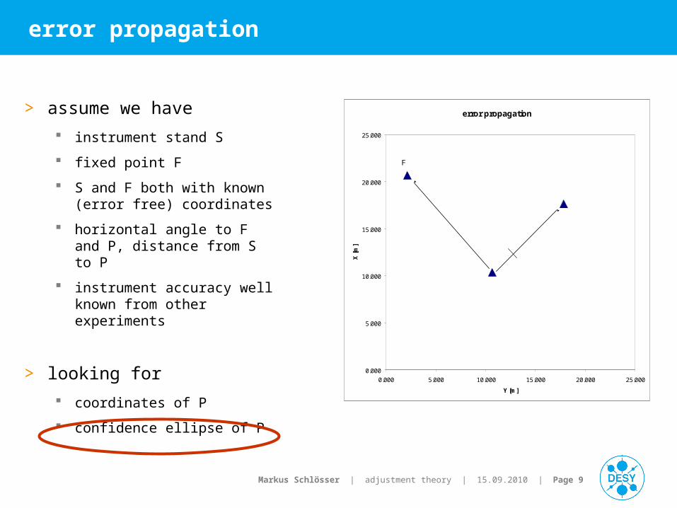
error propagation
> assume we have
instrument stand S
fixed point F
S and F both with known (error free) coordinates
horizontal angle to F and P, distance from S to P
instrument accuracy well known from other experiments
> looking for
coordinates of P
confidence ellipse of P
error propagation
0.000
5.000
10.000
15.000
20.000
25.000
0.000 5.000 10.000 15.000 20.000 25.000
Y [m]
X [
m]
F
S
P

Markus Schlösser | adjustment theory | 15.09.2010 | Page 10
error propagation
mm
mgon
d
r
2.0
3.0
)(
sin
cosX
trr
trrd
Y
X
Y
XZ
SFSFSP
SFSFSPSP
S
S
P
P
gon356.2119tSF
P
2.14520.673F
10.64210.332S
Y [m]X [m]Point
m10.2486dSP [m]gon14.9684=rSP [gon]=Xgon321.6427rSF [gon]
ParametersObservations
Unknowns
m17.836YP [m]
m17.631=
XP [m]= Z
standard deviation of observations
4
9
9
10 8
2
2
2
d
r
r
LL
Variance / Covariance Matrix
Markus Schlösser | adjustment theory | 15.09.2010 | Page 11
error propagation
SPSPSF
SPSPSF
drr
drrF
222
111
SFSFSPSPS trrdX cos1
SFSFSPSPSSFSFSPSPS
SF
trrdXtrrdX
r
2cos
2cos
1
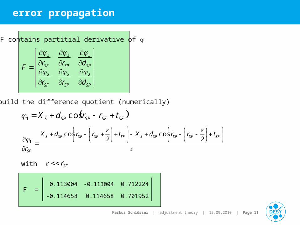
0.7019520.114658-0.114658
0.712224-0.1130040.113004=F
F contains partitial derivative of
build the difference quotient (numerically)
with SFr

Markus Schlösser | adjustment theory | 15.09.2010 | Page 12
error propagation
TLLZZ FF
mmq
mmq
yyy
xxx
15.0
15.0
22
22
42
1
42
1
xyyyxxyyxxH
xyyyxxyyxxH
qqqqqB
qqqqqA
0.0220760.017666
0.0176660.022589ZZ =
covariance matrix of unknowns
variances of coordinates are on the main diagonal
BUT, this information is incomplete and could even be misleading, better use Helmert‘s error ellipse:
qyyqxy
qxyqxx
xy
yyxx
q
2arctan2
1

Markus Schlösser | adjustment theory | 15.09.2010 | Page 13
error propagation
210.9299.0,2
2
H
H
H
BB
AA
99.0
299.0,299.0
299.0,299.0
or even better, use a confidence ellipse. That means that with a chosen probablity Pthe target point is inside this confidence ellipse.
P = 0.99 (=99%)
Quantil of -distribution, with 2 degrees of freedom
A0.99 = 0.61mm
B0.99 = 0.21mm
= 50gon
error propagation
0.000
5.000
10.000
15.000
20.000
25.000
0.000 5.000 10.000 15.000 20.000 25.000
Y [m]
X [
m]
F
S
Psy
sxA
B

Markus Schlösser | adjustment theory | 15.09.2010 | Page 14
network adjustment
Example:
Adjustment of a 2D-network with angular and distance measurements

Markus Schlösser | adjustment theory | 15.09.2010 | Page 15
adjustment theory
> f = 0
no adjustment, but error propagation possible
no control of measurement
> f > 0
adjustment possible
measurement is controlled by itself
f > 100 typical for large networks
> f < 0
scratch your head

Markus Schlösser | adjustment theory | 15.09.2010 | Page 16
network adjustment
Network
0.000
1.000
2.000
3.000
4.000
5.000
6.000
7.000
8.000
9.000
10.000
0.000 5.000 10.000 15.000 20.000 25.000 30.000
Y [m]
X [
m]
S1 S2 S3
N1
N2
N7
N8N4
N3
N6
N5
25.0005.000S315.0005.000S2
5.0005.000S130.00010.000N830.0000.000N720.00010.000N620.0000.000N510.00010.000N410.0000.000N3
0.00010.000N20.0000.000N1
Y [m]X [m]Name small + regular network 2D for easier solution and smaller matrices 3 instrument stands (S1, S2, S3) 8 target points (N1 … N8) all points are unknown (no fixed points) initial coordinates are arbitrary, they just have to
represent the geometry of the network

Markus Schlösser | adjustment theory | 15.09.2010 | Page 17
network adjustment - input
3
2
1
3
3
1
1
8
8
1
1
1,25
S
S
S
S
S
S
S
N
N
N
N
o
o
o
Y
X
Y
X
Y
X
Y
X
X
83
33
82
12
61
11
83
33
82
12
61
11
1,40
NS
NS
NS
NS
NS
NS
NS
NS
NS
NS
NS
NS
d
d
d
d
d
d
r
r
r
r
r
r
L
0
0
0
25
5
5
5
30
10
0
0
1,25
0
X
vector ofunknowns
vector of observations
vector ofcoarse coordinates
mm
mgon
d
r
2.0
3.0
1,40
vector ofstandard deviations

Markus Schlösser | adjustment theory | 15.09.2010 | Page 18
network adjustment
)( 00 XLLLl
382
38
211
211
338
38
111
11
arctan
arctan
)(
SNSN
SNSN
SSN
SN
SSN
SN
YYXX
YYXX
oYY
XX
oYY
XX
XL

Markus Schlösser | adjustment theory | 15.09.2010 | Page 19
network adjustment – design matrix
3
83
1
83
3
83
3
83
1
83
1
83
3
33
1
33
3
33
3
33
1
33
1
33
3
82
1
82
3
82
3
82
1
82
1
82
3
12
1
12
3
12
3
12
1
12
1
12
3
61
1
61
3
61
3
61
1
61
1
61
3
11
1
11
3
11
3
11
1
11
1
11
3
83
1
83
3
83
3
83
1
83
1
83
3
33
1
33
3
33
3
33
1
33
1
33
3
82
1
82
3
82
3
82
1
82
1
82
3
12
1
12
3
12
3
12
1
12
1
12
3
61
1
61
3
61
3
61
1
61
1
61
3
11
1
11
3
11
3
11
1
11
1
11
25,40
S
NS
S
NS
S
NS
S
NS
N
NS
N
NS
S
NS
S
NS
S
NS
S
NS
N
NS
N
NS
S
NS
S
NS
S
NS
S
NS
N
NS
N
NS
S
NS
S
NS
S
NS
S
NS
N
NS
N
NS
S
NS
S
NS
S
NS
S
NS
N
NS
N
NS
S
NS
S
NS
S
NS
S
NS
N
NS
N
NS
S
NS
S
NS
S
NS
S
NS
N
NS
N
NS
S
NS
S
NS
S
NS
S
NS
N
NS
N
NS
S
NS
S
NS
S
NS
S
NS
N
NS
N
NS
S
NS
S
NS
S
NS
S
NS
N
NS
N
NS
S
NS
S
NS
S
NS
S
NS
N
NS
N
NS
S
NS
S
NS
S
NS
S
NS
N
NS
N
NS
o
d
o
d
Y
d
X
d
Y
d
X
d
o
d
o
d
Y
d
X
d
Y
d
X
do
d
o
d
Y
d
X
d
Y
d
X
d
o
d
o
d
Y
d
X
d
Y
d
X
do
d
o
d
Y
d
X
d
Y
d
X
d
o
d
o
d
Y
d
X
d
Y
d
X
do
r
o
r
Y
r
X
r
Y
r
X
r
o
r
o
r
Y
r
X
r
Y
r
X
ro
r
o
r
Y
r
X
r
Y
r
X
r
o
r
o
r
Y
r
X
r
Y
r
X
ro
r
o
r
Y
r
X
r
Y
r
X
r
o
r
o
r
Y
r
X
r
Y
r
X
r
A

Markus Schlösser | adjustment theory | 15.09.2010 | Page 20
network adjustment
A-Matrix has lots of zero-elements
Network points instrument standsorientationunknowns

Markus Schlösser | adjustment theory | 15.09.2010 | Page 21
network adjustment
1LLQP
P is a diagonal matrix, because we assume that observations are uncorrelated

Markus Schlösser | adjustment theory | 15.09.2010 | Page 22
network adjustment
25,4040,4025,4025,25APAN T
• Normal matrix shows dependencies between elements• Normal matrix is singular when adjusting networks without fixed points
• easy inversion of N is not possible• network datum has to be defined• add rows and colums, to make the matrix regular

Markus Schlösser | adjustment theory | 15.09.2010 | Page 23
network adjustment
3
3
1
1
10
01
10
01
S
S
N
N
X
Y
X
Y
G
• datum deficiency for 2D-network with distances:• 2 translations• 1 rotation
• minimize the total matrix trace means to put the network on all point coordinates• additional rows and columns look as
Constraints:
0ˆˆ
0ˆ
0ˆ
00
iiii
i
i
yXxY
y
x No shift of network in x
No shift of network in y
No rotation of network around z

Markus Schlösser | adjustment theory | 15.09.2010 | Page 24
network adjustment
• after addition of G, Normalmatrix is regular and thus invertible
• N-1 is in general fully occupied

Markus Schlösser | adjustment theory | 15.09.2010 | Page 25
network adjustment
1,4040,4025,401,25lPAn T
1,25
1
25,251,25
ˆ nNx

Markus Schlösser | adjustment theory | 15.09.2010 | Page 26
network adjustment
xXX ˆˆ 0
1ˆˆ
NQXX
adjusted coordinates and orientation unknowns
information about the error ellipses

Markus Schlösser | adjustment theory | 15.09.2010 | Page 27
network adjustment
XX
Q ˆˆ
11NNQ

Markus Schlösser | adjustment theory | 15.09.2010 | Page 28
network adjustment
112011 NNNN Qs
qyyqxy
qxyqxx
2299.0,15,299.0
2299.0,15,299.0
4
4
xyyyxxyyxx
xyyyxxyyxx
qqqqqFB
qqqqqFA
xy
yyxx
q
2arctan2
1
XXXXQs ˆˆ20ˆˆ
building the covariance matrix of unknowns (with empirical s02)
2D-Network
degrees of freedom
error probability 1-

Markus Schlösser | adjustment theory | 15.09.2010 | Page 29
network adjustment
error ellipses with P=0.01 error probability for all network points

Markus Schlösser | adjustment theory | 15.09.2010 | Page 30
network adjustment
Network
0,000
1,000
2,000
3,000
4,000
5,000
6,000
7,000
8,000
9,000
10,000
0,000 5,000 10,000 15,000 20,000 25,000 30,000
Y [m]
X [m
]
S1 S2 S3
N1
N2
N7
N8
confidence ellipses for all network pointsrelative confidence ellipses beewen some network points
Markus Schlösser | adjustment theory | 15.09.2010 | Page 31
network adjustment
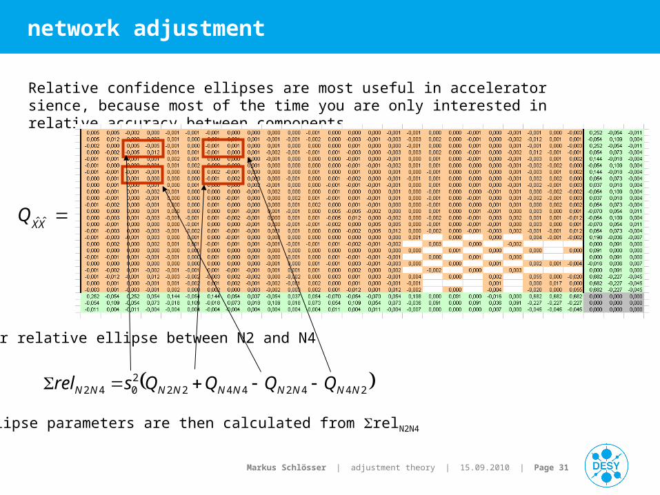
Relative confidence ellipses are most useful in accelerator sience, because most of the time you are only interested in relative accuracy between components.
XX
Q ˆˆ
For relative ellipse between N2 and N4
244244222042 NNNNNNNNNN QQQQsrel
Ellipse parameters are then calculated from relN2N4

Markus Schlösser | adjustment theory | 15.09.2010 | Page 32
network adjustment
0
!
0
0
0
20
0010.0
0012.0
ˆ
s
sun
Pvvs
lxAvT
estimation of s02 from corrections v
23.544.10.1
2.1
~
2
2
21,2
0
20
f
s is used as a statistical test, to proof that the model parameters are right
à priori variances are ok, with P = 0.99

Markus Schlösser | adjustment theory | 15.09.2010 | Page 33
adjustment
Example:
2D - ellipsoid fiddeviation of position and rotation of an ellipsoidal flange

Markus Schlösser | adjustment theory | 15.09.2010 | Page 34
flange adjustment
mmB
mmA
50
80
gon
mm
mm
Y
X
X
0
0
0
0
0
0
0
6
6
1
1
P
P
P
P
Y
X
Y
X
L
known parameters(e.g. from workshop drawing)
01
cos)(sin)(sin)(cos)(2
200
2
200
B
YYXX
A
YYXX iiii
unknowns with initial value
Observations
constraints

Markus Schlösser | adjustment theory | 15.09.2010 | Page 35
flange adjustment
Since it is not (easily) possible to separate unknowns and observations in the constraints,we use the general adjustment model:
0ˆ0
w
x
k
A
ABBQT
TLL
B contains the derivative of with respect to LA contains the derivative of with respect to Xk are the Lagranges Multiplicators (“Korrelaten”)x is the vector of unknownsw is the vector (L,X0)

Markus Schlösser | adjustment theory | 15.09.2010 | Page 36
flange adjustment
B
0T
TLL
A
ABBQ
A

Markus Schlösser | adjustment theory | 15.09.2010 | Page 37
flange adjustment
11.08.1
346.1
299.0,22
0
20
0
s
s
Result:
4.0
45
20.0
22.0
9.4
7.0
9.10
0
flange
ell
flange
gon
mmB
mmA
mmY
mmX

Markus Schlösser | adjustment theory | 15.09.2010 | Page 38
the end for now
may your [vv] always be minimal …