Adjoint-Based Optimization of a Hypersonic Inlet · on the solid surface of a scramjet inlet to accelerate Monte-Carlo characterization of the probability of unstart. The contributions

Adjoint-Based Optimization of a Hypersonic Inlet

Heather Kline∗

Stanford University, Stanford, CA 94305, U.S.A.

Francisco Palacios†

The Boeing Company, Long Beach, CA 90808, U.S.A.

Thomas D. Economon‡, and Juan J. Alonso§

Stanford University, Stanford, CA 94305, U.S.A.

Supersonic combustion ramjets, or scramjets, have the potential to facilitate more ef-ficient transatmospheric flight and airplane-like operations of launch vehicles. A scramjetis an airbreathing engine which uses the compression of air over the forebody and in-let to achieve the conditions necessary for supersonic combustion, using no mechanicalcompressor. The highly complex flow experienced by three-dimensional hypersonic inlets,demanding performance requirements, and engine design strongly coupled to the vehiclecreate a need for simulation-based design. Therefore, efficient high-fidelity computationof gradients is desired. In this paper, the derivation, verification, and application of anadjoint formulation for an objective relevant to thrust (m) will be presented. The designproblem addressed is the optimization of a simple hypersonic inlet geometry, however thismethod is applicable to other engineering problems.

Student Paper Competition Entry.

Nomenclature

V ariable Definition

~Ac convective jacobian~Av viscous jacobianF flux vectorJ objective functionJ lagrangianU vector of conservative variablesV vector of primitive variablesΨ vector of adjoint variablesM transformation matrix between conservative and primitive flow variablesL matrix of left eigenvectors of the Jacobiang generic functionΛ diagonal matrix of Jacobian eigenvaluesΩ fluid volume domainΓe outlet boundary of the fluid domainΓi inlet boundary of the fluid domainS solid wall boundary~t unit tangent vector~n unit normal vector

∗Ph.D. Candidate, Department of Aeronautics & Astronautics, AIAA Student Member.†Engineer, Advanced Concepts Group, AIAA Senior Member.‡Postdoctoral Scholar, Department of Aeronautics & Astronautics, AIAA Senior Member.§Professor, Department of Aeronautics & Astronautics, AIAA Associate Fellow.

1 of 24

American Institute of Aeronautics and Astronautics

Dow

nloa

ded

by T

hom

as E

cono

mon

on

July

15,

201

5 | h

ttp://

arc.

aiaa

.org

| D

OI:

10.

2514

/6.2

015-

3060

22nd AIAA Computational Fluid Dynamics Conference

22-26 June 2015, Dallas, TX

AIAA 2015-3060

Copyright © 2015 by Heather Kline, Francisco Palacios, Thomas Economon, Juan Alonso. Published by the American Institute of Aeronautics and Astronautics, Inc., with permission.

AIAA Aviation

x, y, z cartesian coordinates~v velocity vectoru, v, w cartesian components of velocityE total energyH total enthalpyM0 freestream Mach numberc speed of soundα normal boundary deformationρ densityP static pressureT temperatureγ ratio of specific heatsf fuel:air ratio

Subscripts

0 freestream2 entrance to isolator, end of inlet3 end of isolator, entrance to combustor4 exit of combustor10 end of nozzle/ expansion rampb burnert total, or stagnation state

Mathematical symbols

∇ nabla, gradient operator∇tg tangent derivative on a surface∂ partial derivative∂n normal derivative to a curve∂tg tangent derivative to a curve∂x ∂/∂xδ first variation

Units

Pa Pascalsm meterss seconds

I. Introduction and Motivation

Supersonic combustion ramjets, or scramjets, have the potential to facilitate more efficient transatmo-spheric flight and airplane-like operations of launch vehicles. A scramjet is an airbreathing engine which

uses the compression of air over the forebody and inlet to achieve the conditions necessary for supersoniccombustion, using no mechanical compressor. These engines operate in hypersonic conditions, ranging fromMach 5 to Mach 10 at current levels of technology. Ramjets have flown up through Mach 5.5, and at Machnumbers of around that magnitude it becomes more efficient to use supersonic combustion.1 Recent flighttests of the HIFiRE, X-51 and X-43A have had success in achieving positive thrust, while also highlightingthe difficulties of designing hypersonic airbreathing engines.1–3 The highly complex flow experienced bythree-dimensional hypersonic inlets, demanding performance requirements, and engine design strongly cou-pled to the vehicle create a need for simulation-based design. Therefore, efficient high-fidelity computationof gradients is desired. In this paper, the derivation, verification, and application of an adjoint formulationfor an objective relevant to thrust (m) will be presented. The design problem addressed is the optimizationof a simple hypersonic inlet geometry, however this method is applicable to other engineering problems.

There is ample existing work in the design of inviscid inlets. The simplest design is a two-dimensional sin-

2 of 24


Dow

nloa

ded

by T

hom

as E

cono

mon

on

July

15,

201

5 | h

ttp://

arc.

aiaa

.org

| D

OI:

10.

2514

/6.2

015-

3060

gle ramp which forms two shocks- the first extending from the nose of the vehicle and meeting the cowl, andthe other returning the flow to the horizontal direction. More efficient is the Busemann diffuser4 which usesa surface designed to result in the Mach waves meeting at a single point, and forming a conical shock whichreturns the flow to horizontal, as illustrated in Figure 1. This design achieves much of the compression isen-tropically, resulting in lower stagnation pressure losses. Building off of the Busemann flowfield, streamtracingtechniques5 allow more complex geometries, for example transitioning from a rectangular cross-section atthe entrance to a circular cross-section at the combustor to gain benefits from simpler vehicle integrationand lower weight combustors. Rectangular-to-Elliptical-Shape-Transition (REST) inlets with boundary layercorrections further build on these concepts.6 However, even a REST inlet with boundary layer correctionsmay not achieve the designed performance,7 due to the complex interactions of shocks and boundary layersin a complex internal hypersonic flow.

Figure 1: Flowfield of a full Busemann diffuser. Image reproduced from [8].

Modern simulation techniques allow for more efficient high fidelity optimization. Advances in computerspeed and efficiency make it possible to complete more function evaluations than previous, however the cputime required for high-fidelity optimization with large number of design variables is still significant. Moreefficient calculation of the gradient of the objective function(s) can significantly reduce the time required foroptimization. The adjoint method introduced by Jameson9 provides a more efficient method of calculatinggradients, which is independent of the step size and of the number of design variables. An adjoint solutionuses information from the direct, or flow solution, to solve a new partial differential equation system whichproduces analytical gradients to infinitesimal deformations of the surface. The gradients with respect tochanges in freestream conditions can be found from the same adjoint solution. Adjoints have been applied toscramjet designs in the past, specifically Wang10 et al. used a discrete adjoint for a pressure-based functionalon the solid surface of a scramjet inlet to accelerate Monte-Carlo characterization of the probability of unstart.

The contributions of this paper are the implementation of a continuous adjoint for the off-body objectivefunction that is the mass flow rate through the outlet, verification by comparison to finite difference, andoptimization of simple geometry in inviscid and viscous flows. This builds on previous work by the authors,11

which used finite difference methods to evaluate the change in performance for a thermoelasticaly deformedinlet, for an objective function of interest to a similar design problem. This paper will begin with a descriptionof the physical problem and generic scramjet geometry followed by the methods used in this work, includingthe derivation of the adjoint for a mass flow rate objective function will be summarized. The results ofverification and optimization cases using this objective function will be shown.

3 of 24


Dow

nloa

ded

by T

hom

as E

cono

mon

on

July

15,

201

5 | h

ttp://

arc.

aiaa

.org

| D

OI:

10.

2514

/6.2

015-

3060

II. Description of the Physical Problem

Hypersonic Airbreathing Engines

Hypersonic flow begins in the neighborhood of Mach 5, and is defined not with a specified Mach numberbut as the flight regime where a number of physical phenomena become more significant. These phenomenainclude thin shock layers where the shock lies very close to the surface of the vehicle, thick boundary layerswhich interact with the shocks and a large entropy gradient, and the possibility of chemically reacting flowand real gas effects.12 In terms of the effect on vehicle design, around Mach 5 the cost of decelerating airto subsonic speeds begins to outweigh the cost of supersonic combustion. Combustion at supersonic speedsis more difficult to implement, and issues with residence time, sufficient mixing, and unstart become moresignificant. The inlets of scramjets need to compress the air sufficiently, while maintaining low drag andhigh efficiency. Under extreme pressure and heat, there is a higher degree of shape uncertainty. Hypersonicvehicles for access to space are required to operate under a very large range of flight conditions, acceleratingto an altitude where rocket propulsion takes over. A diagram of a scramjet is shown in Figure 2. This figurealso identifies the stations 0-10 which will be used as subscripts to describe the state of the flow at thoselocations. Several numbers are left out of this figure for consistency with describing other engines, wherethere would be more components between the exit of the combustion chamber or burner and the nozzle.

Figure 2: Scramjet flow path. Reproduced from Figure 1 of [13]

Several quantities of interest could be used for optimization. The choice of objective function will stronglydetermine the outcome. For inlet optimization, the stagnation pressure is often maximized, and there areseveral other options related to scramjet performance such as the kinetic energy efficiency as described bySmart.13 In this work, we will be optimizing the mass flow rate, which is directly related to the thrust of theengine. The equation for thrust is shown in Equation 1 and is based on the momentum flux of the air passingthrough the engine. The derivation of this equation can be found in [14]. The quantities with subscript 0 arethe freestream values, and the quantities with subscript 10 are values at the exit of the expansion ramp, asshown in Figure 2. In this equations M is the Mach number, P is the static pressure, T is the temperature,f is the mass flow fraction of fuel:air, c indicates the speed of sound, m is the mass flow rate, and subscriptsindicate the location along the flowpath as shown in Figure 2.

Fx = m0c0M0

((1 + f)

M10

M0

√T10

T0− 1

)+A10

A0

(P10

P0− 1

)(1)

For the purposes of this work, we would like to optimize this inlet without needing to calculate the valuesthrough the combustor. While the values at station 10 will be dependent on several other quantities whichcould be calculated on the inlet, the mass flow rate is an intuitive and simple quantity to use in this case.In Section III, we will see that this choice of objective function results in a very simple formulation.

Model Case

The flight conditions chosen are Mach 7.0 with a freestream temperature of 221.9 degK, and freestream staticpressure of 2183.37Pa. These conditions correspond to conditions used in previous work11 for verification.The resulting Reynolds number for an inlet of 1.0 meter is about 5 × 106. These conditions correspond

4 of 24


Dow

nloa

ded

by T

hom

as E

cono

mon

on

July

15,

201

5 | h

ttp://

arc.

aiaa

.org

| D

OI:

10.

2514

/6.2

015-

3060

to 75kPa at Mach 7. Undersped cases have a Mach number of 5.0 and the same freestream pressure andtemperature.

A simple two-dimensional geometry used to verify adjoint results and as an initial point for optimization.This geometry was designed using oblique shock equations15 such that the shock resulting from the angle ofthe ramp meets the cowl lip. The height of the isolator and length of the cowl are designed such that thesecond shock impinges at the end of the ramp, leading to horizontal flow at the isolator. The parameters ofthis design are a desired static pressure ratio of 20.0, a design Mach number of 7.0, and an inlet length of 1.0meters. A schematic and dimensions are also included in the appendix. The geometry is shown in Figure 3.The nose and cowl have been filleted to have a radius of 0.0005 meters in order to avoid sharp edges.

Additional volume required for deformation of mesh.

Nose

Isolator

Outlet

Farfield

Cowl lip

Figure 3: Baseline geometry used as initial point in optimization and for verification of adjoint method.

At Mach 7 in inviscid flow, this design is expected to be a local maximum for mass flow rate, if the heightbetween the nose and cowl remains constant. Due to the supersonic nature of the flow if the leading shock(starting at the cowl lip) moves further downstream towards the isolator the mass flow rate should remainconstant. If that shock is moved upstream from the cowl the flow will spill out around the cowl, reducingthe mass flow rate. When viscous effects are included or when at off-design conditions this shape will notbe an optimum. At off-design conditions of a lower Mach number the mass flow rate can be increased bymoving the shock closer to the cowl lip. The straight ramp design is chosen as the initial point rather thana Busemann flow field for its simplicity.

For three-dimensional simulations the two-dimensional geometry is extruded to have a width of 0.1 meters.This geometry is simulated as symmetric about the center of the inlet, and the actual geometry simulatedhas a width of 0.05 meters. Side walls are added to complete this geometry, connecting the nose to thecowl. Once again, the edges of this geometry have been rounded with a radius of 0.0005 meters to avoidsharp edges in the simulation, which can cause convergence issues16 as well as increasing the likelihood ofoverlapping geometry when deformations are applied. This geometry is illustrated in Figure 4.

III. Adjoint Derivation With An Off-Body Objective Function

A continuous adjoint problem, using information from the direct, or flow solution, solves a new partialdifferential equation system which produces analytical gradients to infinitesimal deformations of the surface.These sensitivities can be projected into any arbitrary deformation. The gradients with respect to changesin freestream conditions can be found from the same adjoint solution. This method requires a secondPDE system and the derivation of boundary conditions that depend on the objective function of interest.While a new set of boundary conditions is required for every new objective function, this method providesgradients for an arbitrary number of design variables for approximately the same computational cost asa single additional direct solution. By comparison, the finite difference method of calculating gradients

5 of 24


Dow

nloa

ded

by T

hom

as E

cono

mon

on

July

15,

201

5 | h

ttp://

arc.

aiaa

.org

| D

OI:

10.

2514

/6.2

015-

3060

Figure 4: Three-dimensional baseline geometry.

requires an additional direct solution for every additional design variable. A great deal of literature existson adjoints and their derivation. The method was introduced by Jameson,9 and further work by Giles &Pierce,17 Castro18 et al., Hayashi19 et al., and Economon20 provide additional details for the derivation andsolution of adjoints. This work adds the derivation for the boundary conditions for the off-body functionalm. The outlet objective function for total pressure has been developed previously by Papadimitriou &Giannakoglou,21 using a similar process.When an adjoint is derived for an objective function, J , defined on some surface other than a solid body, itis called an off-body functional - for example, the mass flow rate m defined on the exit plane of an inlet. Inthese equations, U refers to the vector of conservative variables, F is the vector of fluxes, Ac is the convectivejacobian, V is the vector of primitive variables, and M is the transformation matrix between the conservativeand primitive variables. W is the vector of characteristic variables, which are constant along characteristicsof these equations. Ψ is the vector of adjoint variables. The adjoint variables, Ψ = (ψρ, ψ

T~ρv, ψρE)T are

Lagrange operators for the direct system of equations, in this case the Euler Equations. Ω represents thevolume.

Let us assume the objective function is defined as an integral over an outlet surface Γe. Equation 2 showsthis integral for the objective function of m. For generality the term g will be used for intermediate steps ofthe derivation, and expanded when necessary.

J =

∫Γe

gds =

∫Γe

ρ~v · ~nds (2)

Our goal is to find ∂J∂S , where S is the surface to be designed. In order to find this value, we set up a

variational problem under the constraint that the variations of the flow variables must satisfy the directionproblem. This constraint is satisfied by setting the variation of the residual R(U) to zero. R(U) is expandedfor the steady Euler Equations in Equations 3-4.

R(U) = ∇ · ~F =∂

∂t(U) +∇ · ~AU

δR(U) = ∇ · ~AδU(3)

The Jacobian Ac is expanded in the appendix. The conservative variables U and primitive variables Vare defined as:

6 of 24


Dow

nloa

ded

by T

hom

as E

cono

mon

on

July

15,

201

5 | h

ttp://

arc.

aiaa

.org

| D

OI:

10.

2514

/6.2

015-

3060

U =

ρ

ρ~v

ρE

, V =

ρ

~v

P

. (4)

The Lagrangian is defined in Equation 5, where the adjoint variables Ψ are introduced as the Lagrangemultipliers in the application of the constraint.

J = J −∫

Ω

ΨTR(u)dΩ

δJ = δJ −∫

Ω

ΨT δR(U)dΩ

(5)

In order to solve this problem for the sensitivity ∂J∂S , which will be equated to δJ

δS , we need to eliminatedependence on δU . This is accomplished first through linearizing the governing equations and applying knownrelationships between variables from the direct problem, and then through applying boundary conditionsthat eliminate the remaining undesired variational terms. The linearization of the governing equations andtheir boundary conditions is shown in Equation 6. The variation of characteristic variables along the positivecharacteristics is zero, the velocity is tangent to the wall, and the variation of the residual is zero.

δR = ∇ · ~AδU = 0 in Ω

δ~v = −∂n(~v) δS on S

(δW )+ = 0 on Γ∞

(6)

The variation of J is expanded in Equation 7. It is reasonable to assume for this problem that the outletsurface will be undeformed, such that the term δΓe can be set to 0. For functional defined on the solid bodybeing designed, these terms cannot be set to 0.

δJ =

∫δΓe

g(U)ds+

∫Γe

∂g

∂UδUds∫

δΓe

g(U)ds =

∫Γe

∂g(U)

∂U(δS · ∇U)ds+

∫Γe

g(U)δds = 0

δJ =

∫Γe

∂g

∂UδUds =

∫Γe

∂g

∂VδV ds

(7)

Applying the Divergence Theorem, the expression for δJ in Equation 5 can be rewritten as shown inEquation 8. In these equations Γ refers to the open boundary (farfield, inlet, and exit boundaries), S refersto the solid surface, and Γe refers to the boundary over which m is calculated. Γe overlaps with Γ.

δJ = δJ −∫

Ω

ΨT δR(U)dΩ∫Ω

ΨT δR(U)dΩ =

∫Γ

ΨT ~A · ~nδUds+

∫S

ΨT ~A · ~nδUds+

∫S

ΨT ~A · ~nδSds−∫

Ω

∇ΨT ~AδUdΩ

δJ =

∫Γe

∂g

∂UδUds−

∫Γ

ΨT ~A · ~nδUds−∫S

ΨT ~A · ~nδUds−∫S

ΨT ~A · ~nUδSds+

∫Ω

∇ΨT ~AδUdΩ

(8)

We can now express the adjoint problem as shown in Equation 9, where the integral over the volume fromEquation 8 defines the PDE to solve, and the integrals over the boundaries of the domain (Γ, S) providethe boundary conditions. A shorthand term is introduced for the momentum components of the adjointvariables, ~ϕ = ψρu, ψρv, ψρwT . For convenience, the primitive variables V will now be used.

−∇ΨT · ~A = 0 in Ω∂g∂V δV −ΨT ~A · ~nMδV = 0 on exit surface Γe

ΨT ~A · ~nMδV = 0 on open boundaries Γ 6= Γe

~ϕ = −ψρE~v on solid walls S

(9)

7 of 24


Dow

nloa

ded

by T

hom

as E

cono

mon

on

July

15,

201

5 | h

ttp://

arc.

aiaa

.org

| D

OI:

10.

2514

/6.2

015-

3060

The terms at the outlet are expanded for the mass flow rate objective function in Equation 10. The termvn = ~v · ~n.

∂g

∂VδV −ΨT ~A · ~nMδV = 0

vnδρ+ ρ~n · δ~v −

ψρvn + ~v · ~ϕvn + ψρEvn

(~v2

2

)ρ(~v · ~ϕ)~n+ ρvn~ϕ+ ρψρ~n+ ψρE(ρvn~v + ρ( c2

γ−1 + γ ~v2

2 )~n

~ϕ · ~n+ ψρE(vnγγ−1 )

T

δρ

δ~v

δP

= 0

(10)

Under subsonic conditions, the pressure at the outlet is specified and therefore δP = 0. Eliminating thedependence on the remaining, arbitrary, variations leads to Equation System 11.

vn −(ψρvn + ~v · ~ϕvn + ψρEvn

(~v2

2

))= 0

ρ~n−(~n

(ρ(~v · ~ϕ) + ρψρ + ψρEρ

(c2

γ − 1+ γ

~v2

2

))+ ~ϕ (ρvn) + ~v (ψρEρvn)

)= ~0

(11)

The boundary condition at the outlet in terms of the energy adjoint variable reduces to Equation 12.When the exit experiences supersonic flow, δP becomes arbitrary, introducing an additional equation whichis satisfied when ψρE = 0. This reduces the boundary condition to Equation 13. Equations 12 and 13are the critical result of this derivation, and of this work. Applying this boundary condition, along with theconditions at boundaries not included in the objective function, result in the ability to find the variationof m with respect to the normal variation of the surface δS. The correctness of the assumptions made inthe derivation of these equations, and their implementation, will be tested in the verification section of thiswork.

ψρ

~ϕ

ψρE

Γe,Me<1

=

ψρE

(c2

γ−1 + |~v|22

)+ 1

ψρE

(−c2

~v·~n(γ−1)~n− ~v)

ψρE

(12)

ψρ

~ϕ

ψρE

Γe,Me>1

=

1~0

0

(13)

For the viscous case Equation 14 could be applied to account for perturbations of the eddy viscosity,however it will be neglected for this work. This simplification is also assumed at farfield boundaries, andis the convention for continuous adjoints. Viscous terms do appear in the volume integral and at solidboundaries in the adjoint formulation for viscous flow.

ψT ( ~Av)δV · ~n+ ψT δ

·¯σ

¯σ · ~v

· ~n+ ψT δ

··

µ2totcp∇T

· ~n+ ~n ·(Σϕ + ΣψρE~v

)− ∂g

∂VδV = 0 (14)

At the inlet to the computational volume, the boundary condition is defined by∫

Γi(ΨT ~A · ~nδU)ds = 0.

In supersonic flow, all of the characteristic are exiting, leading to the condition that the adjoint variables areinterpolated from the volume solution as the iterative solution progresses. At farfield boundaries we assumethat the variations of the conservative variables, δU are negligible, which is consistent with the boundarycondition of the direct problem.

After application of the boundary conditions that eliminate the dependence on the variation in theconservative variables δU , and assuming only normal deformations, the remaining terms on the surface inEquation 8 can be reduced to the terms shown in Equation 15, defining the surface sensitivity, ∂J

∂S , whichis multiplied by the normal deformation δS in Equation 15. A full derivation of this term can be found inwork by Castro.18

8 of 24


Dow

nloa

ded

by T

hom

as E

cono

mon

on

July

15,

201

5 | h

ttp://

arc.

aiaa

.org

| D

OI:

10.

2514

/6.2

015-

3060

δJ =

∫S

∂J

∂SδSds

∂J

∂S= (∇ · ~v)(ρψρ + ρ~v · ψ ~ρv + ρHψρE) + ~v · ∇(ρψρ + ρ~v · ψ ~ρv + ρHψρE)

(15)

The surface sensitivity defined in Equation 15 is defined at every point on the surface assuming a con-tinuous surface and continuous solution to the direct problem. In theory the application of the divergencetheorem during the derivation should require that discontinuities like shocks in the flow should be treateddifferently, e.g., by sensing the shock location and applying an additional boundary condition along thatsurface. In practice, as shocks are not true discontinuities within the numerical flow solution, this is notnecessary and gradients without a shock correction match well with finite difference results. It has also beenassumed that viscous perturbations at the outlet, inlet, and farfield boundary conditions are negligible.

This derivation has focused on the inviscid problem. In the viscous problem, the boundary conditions onthe surface and the equation for the surface sensitivity are modified. At inlet and outlet boundary conditionsthe viscous perturbations are assumed negligible, and these boundary conditions to not change. The equa-tions defining these boundary conditions and the viscous surface sensitivity can be found in Reference [22].Since the viscous perturbations at the outlet are neglected in this work, the boundary conditions developedhere remain unchanged.

IV. Numerical Implementation

Computational Fluid Dynamics

The open-source CFD suite SU2, developed in the Aerospace Design Lab at Stanford University,23 was usedto generate flow solutions and the adjoint solution. A new boundary condition and other modifications wereimplemented in order to produce the continuous adjoint solution for m. The Euler Equations were used inverification and in initial optimization cases. The Reynolds Averaged Navier Stokes equations with the SAturbulence model was used for viscous simulations.

SU2 uses the Finite Volume Method (FVM) to solve partial differential equations including the Reynolds-Averaged-Navier-Stokes (RANS) equations and the Euler equations. This software suite uses unstructuredmeshes to discretize the volume. In the RANS equations, a turbulence model is used to account for theReynolds stresses. The one-equation Spalart-Allmaras and two-equation SST k-omega turbulence modelsare available. The adjoint equations are solved in a similar fashion, re-using methods implemented to solvepartial differential equations and the information generated by the flow solver.

Free-Form Deformation Variables

A Free-Form Deformation (FFD) strategy has also been adopted in both two and three dimensions, whichhas become a popular geometry parameterization technique for aerodynamic shape design.24–26 In FFD, aninitial box encapsulating the object (rotor blade, wing, fuselage, etc.) to be redesigned is parameterized as aBezier solid. A set of control points are defined on the surface of the box, the number of which depends onthe order of the chosen Bernstein polynomials. The solid box is parameterized by the following expression:

X(u, v, w) =

l,m,n∑i,j,k=0

Pi,j,kBlj(u)Bmj (v)Bnk (w), (16)

where u, v, w ∈ [0, 1], and Bi is the Bernstein polynomial of order i. The Cartesian coordinates of thepoints on the surface of the object are then transformed into parametric coordinates within the Bezier box.

The control points of the box become design variables, as they control the shape of the solid, and thus theshape of the surface grid inside. The box enclosing the geometry is then deformed by modifying its controlpoints, with all the points inside the box inheriting a smooth deformation. Once the deformation has beenapplied, the new Cartesian coordinates of the object of interest can be recovered by simply evaluating themapping inherent in Eqn. 16. An example of FFD control point deformation to a wing geometry appears inFig. 5.22

9 of 24


Dow

nloa

ded

by T

hom

as E

cono

mon

on

July

15,

201

5 | h

ttp://

arc.

aiaa

.org

| D

OI:

10.

2514

/6.2

015-

3060

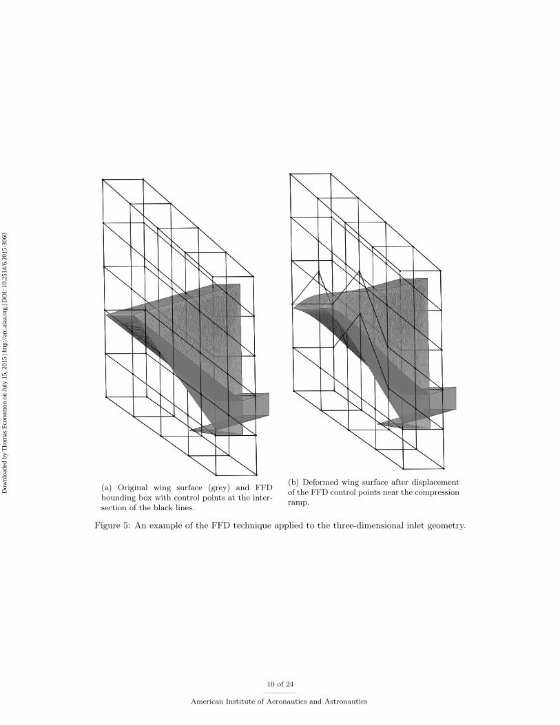
(a) Original wing surface (grey) and FFDbounding box with control points at the inter-section of the black lines.

(b) Deformed wing surface after displacementof the FFD control points near the compressionramp.

Figure 5: An example of the FFD technique applied to the three-dimensional inlet geometry.

10 of 24


Dow

nloa

ded

by T

hom

as E

cono

mon

on

July

15,

201

5 | h

ttp://

arc.

aiaa

.org

| D

OI:

10.

2514

/6.2

015-

3060

Optimization Method

The optimization method used in this work is the fmin slsqp function from the PythonTM version 2.7.6module scipy.optimize. This optimization method is a bounded, gradient based optimization using sequentialleast square programming.27 The adjoint method was used to provide gradients in these optimization results,and the design variables were constrained by a maximum amplitude of 0.1 meters unless otherwise stated.This optimization problem is expressed in Equation 17. The optimizer is also limited to 10 iterations, toreasonably limit the time required and because in the cases presented here the majority of the design gainswere achieved within the first two or three iterations.

V. Results

As this is both a new boundary condition being applied and implemented, verification is required prior toapplication of the results to optimization. In the following sections, verification is presented for the gradientvalues computed by the adjoint method compared to gradients computed by finite difference. Following theverification, the adjoint method was applied to example optimization problems which successfully increasedthe mass flow rate up to the point where the leading shock meets the cowl.

Adjoint Method Verification

In order to verify that the implementation of the adjoint for mass flow rate operates satisfactorily, in thissection we compare the gradients computed with the adjoint method to gradients computed with finitedifferences. This will include two and three dimensional simulations using the Euler equations, and twodimensional simulations using the RANS equations. These results have been selected to be relevant to theoptimization results presented later.

Results for an inviscid case are shown in Figure 7, using the 7 design variables shown in Figure 6. The 0thdesign variable controls the nose length through a horizontal deflection, while the 1st - 6th design variablescontrol the shape of the ramp through vertical deflections. Figure 6 shows all design variables at a positive0.01 deflection.

Figure 6: Illustration of numbered design variables for 7-DV cases. Figure overlays FFD box with undeformed(black/unfilled points) and deformed (red/filled points) control points.

Figure 8 shows a similar trend in the gradients computed for the viscous case, at Mach 7. This figureincludes the gradients computed by finite difference for inviscid flow for comparison. The gradients are notas closely matched as the inviscid results, however the difference is small enough that these gradients maybe used for optimization. The sensitivities are larger for viscous flow, particularly at the design variables inthe middle of the ramp. The trend of higher sensitivity for viscous results is consistent with the results ofKline,11 where a finite difference methodology on a three dimensional geometry indicated greater sensitivityof one-dimensionalized flow quantities in viscous flow as opposed to inviscid flow.

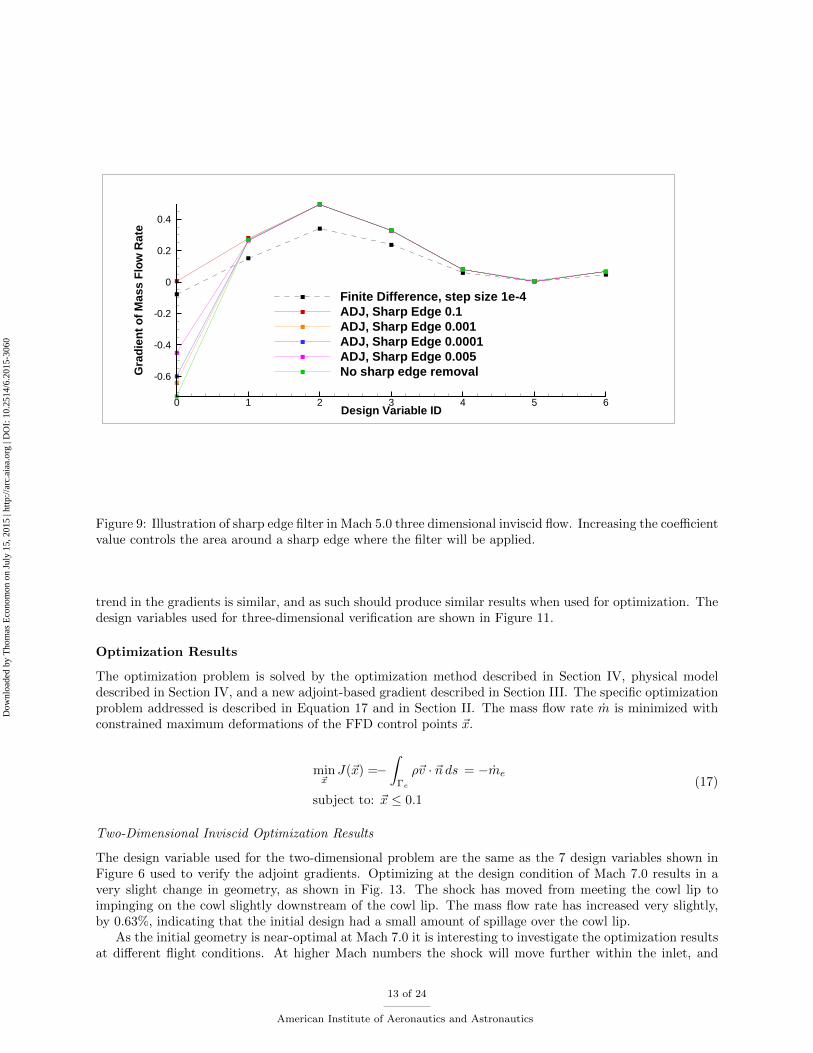
Figure 9 illustrates the effect of using the sharp edge sensitivity removal on the adjoint gradient compu-tation.16 The sharp edge sensitivity removal filters sensitivites near sharp edges where the adjoint solution isexpected to be less accurate, and the distance away from a sharp edge that this filter is applied is controlledby a coefficient. As seen in Figure 9, the sharp edges of the geometry do experience large sensitivities which

11 of 24


Dow

nloa

ded

by T

hom

as E

cono

mon

on

July

15,

201

5 | h

ttp://

arc.

aiaa

.org

| D

OI:

10.

2514

/6.2

015-

3060

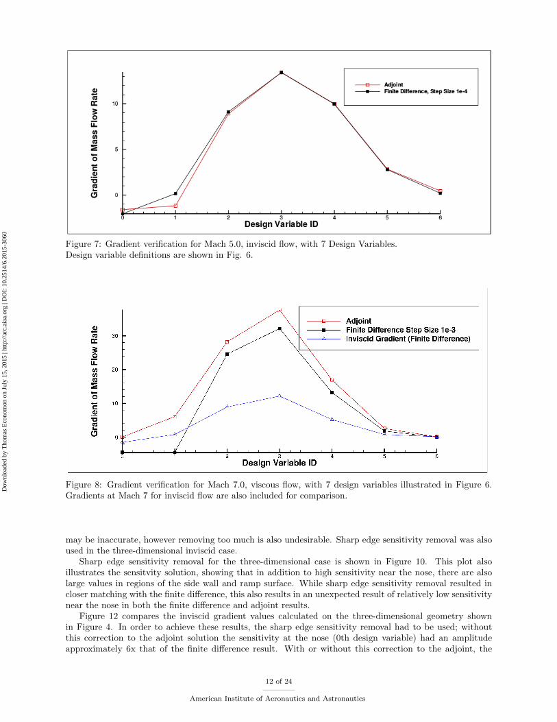
Figure 7: Gradient verification for Mach 5.0, inviscid flow, with 7 Design Variables.Design variable definitions are shown in Fig. 6.

Figure 8: Gradient verification for Mach 7.0, viscous flow, with 7 design variables illustrated in Figure 6.Gradients at Mach 7 for inviscid flow are also included for comparison.

may be inaccurate, however removing too much is also undesirable. Sharp edge sensitivity removal was alsoused in the three-dimensional inviscid case.

Sharp edge sensitivity removal for the three-dimensional case is shown in Figure 10. This plot alsoillustrates the sensitvity solution, showing that in addition to high sensitivity near the nose, there are alsolarge values in regions of the side wall and ramp surface. While sharp edge sensitivity removal resulted incloser matching with the finite difference, this also results in an unexpected result of relatively low sensitivitynear the nose in both the finite difference and adjoint results.

Figure 12 compares the inviscid gradient values calculated on the three-dimensional geometry shownin Figure 4. In order to achieve these results, the sharp edge sensitivity removal had to be used; withoutthis correction to the adjoint solution the sensitivity at the nose (0th design variable) had an amplitudeapproximately 6x that of the finite difference result. With or without this correction to the adjoint, the

12 of 24


Dow

nloa

ded

by T

hom

as E

cono

mon

on

July

15,

201

5 | h

ttp://

arc.

aiaa

.org

| D

OI:

10.

2514

/6.2

015-

3060

Design Variable ID

Gra

dien

t of M

ass

Flo

w R

ate

0 1 2 3 4 5 6

-0.6

-0.4

-0.2

0

0.2

0.4

Finite Difference, step size 1e-4ADJ, Sharp Edge 0.1ADJ, Sharp Edge 0.001ADJ, Sharp Edge 0.0001ADJ, Sharp Edge 0.005No sharp edge removal

Figure 9: Illustration of sharp edge filter in Mach 5.0 three dimensional inviscid flow. Increasing the coefficientvalue controls the area around a sharp edge where the filter will be applied.

trend in the gradients is similar, and as such should produce similar results when used for optimization. Thedesign variables used for three-dimensional verification are shown in Figure 11.

Optimization Results

The optimization problem is solved by the optimization method described in Section IV, physical modeldescribed in Section IV, and a new adjoint-based gradient described in Section III. The specific optimizationproblem addressed is described in Equation 17 and in Section II. The mass flow rate m is minimized withconstrained maximum deformations of the FFD control points ~x.

min~xJ(~x) =−

∫Γe

ρ~v · ~n ds = −me

subject to: ~x ≤ 0.1

(17)

Two-Dimensional Inviscid Optimization Results

The design variable used for the two-dimensional problem are the same as the 7 design variables shown inFigure 6 used to verify the adjoint gradients. Optimizing at the design condition of Mach 7.0 results in avery slight change in geometry, as shown in Fig. 13. The shock has moved from meeting the cowl lip toimpinging on the cowl slightly downstream of the cowl lip. The mass flow rate has increased very slightly,by 0.63%, indicating that the initial design had a small amount of spillage over the cowl lip.

As the initial geometry is near-optimal at Mach 7.0 it is interesting to investigate the optimization resultsat different flight conditions. At higher Mach numbers the shock will move further within the inlet, and

13 of 24


Dow

nloa

ded

by T

hom

as E

cono

mon

on

July

15,

201

5 | h

ttp://

arc.

aiaa

.org

| D

OI:

10.

2514

/6.2

015-

3060

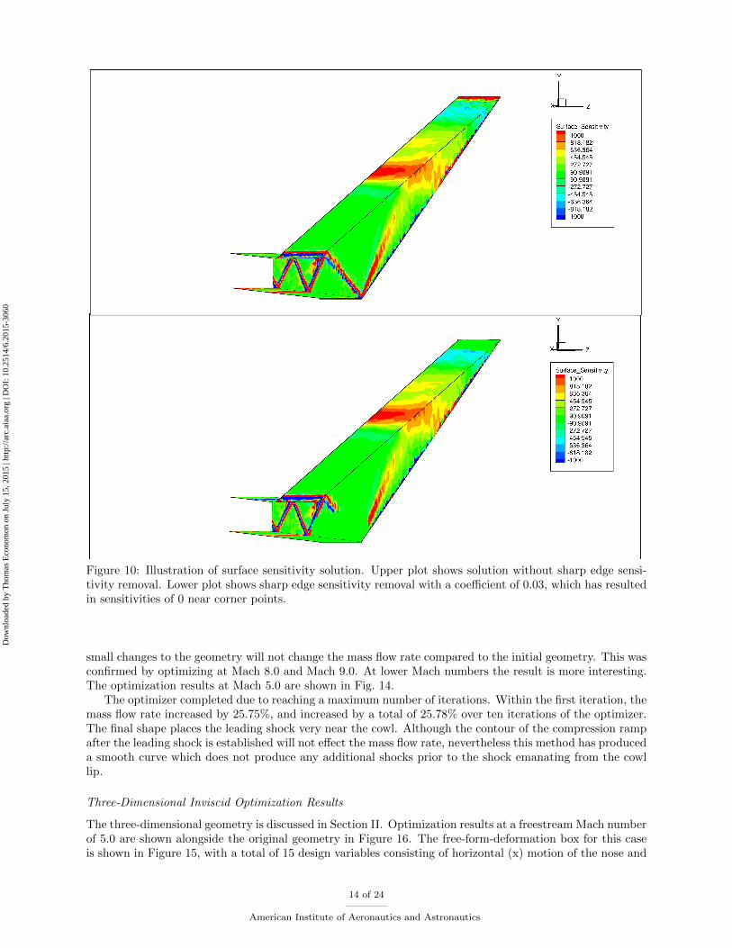
Figure 10: Illustration of surface sensitivity solution. Upper plot shows solution without sharp edge sensi-tivity removal. Lower plot shows sharp edge sensitivity removal with a coefficient of 0.03, which has resultedin sensitivities of 0 near corner points.

small changes to the geometry will not change the mass flow rate compared to the initial geometry. This wasconfirmed by optimizing at Mach 8.0 and Mach 9.0. At lower Mach numbers the result is more interesting.The optimization results at Mach 5.0 are shown in Fig. 14.

The optimizer completed due to reaching a maximum number of iterations. Within the first iteration, themass flow rate increased by 25.75%, and increased by a total of 25.78% over ten iterations of the optimizer.The final shape places the leading shock very near the cowl. Although the contour of the compression rampafter the leading shock is established will not effect the mass flow rate, nevertheless this method has produceda smooth curve which does not produce any additional shocks prior to the shock emanating from the cowllip.

Three-Dimensional Inviscid Optimization Results

The three-dimensional geometry is discussed in Section II. Optimization results at a freestream Mach numberof 5.0 are shown alongside the original geometry in Figure 16. The free-form-deformation box for this caseis shown in Figure 15, with a total of 15 design variables consisting of horizontal (x) motion of the nose and

14 of 24


Dow

nloa

ded

by T

hom

as E

cono

mon

on

July

15,

201

5 | h

ttp://

arc.

aiaa

.org

| D

OI:

10.

2514

/6.2

015-

3060

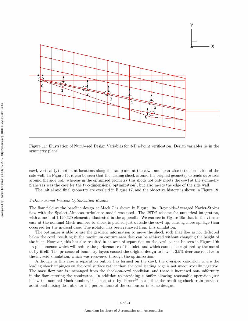
Figure 11: Illustration of Numbered Design Variables for 3-D adjoint verification. Design variables lie in thesymmetry plane.

cowl, vertical (y) motion at locations along the ramp and at the cowl, and span-wise (z) deformation of theside wall. In Figure 16, it can be seen that the leading shock around the original geometry extends outwardsaround the side wall, whereas in the optimized geometry this shock not only meets the cowl at the symmetryplane (as was the case for the two-dimensional optimization), but also meets the edge of the side wall.

The initial and final geometry are overlaid in Figure 17, and the objective history is shown in Figure 18.

2-Dimensional Viscous Optimization Results

The flow field at the baseline design at Mach 7 is shown in Figure 19a. Reynolds-Averaged Navier-Stokesflow with the Spalart-Almaras turbulence model was used. The JST28 scheme for numerical integration,with a mesh of 1,120,620 elements, illustrated in the appendix. We can see in Figure 19a that in the viscouscase at the nominal Mach number to shock is pushed just outside the cowl lip, causing more spillage thanoccurred for the inviscid case. The isolator has been removed from this simulation.

The optimizer is able to use the gradient information to move the shock such that flow is not deflectedbelow the cowl, resulting in the maximum capture area that can be achieved without changing the height ofthe inlet. However, this has also resulted in an area of separation on the cowl, as can be seen in Figure 19b- a phenomenon which will reduce the performance of the inlet, and which cannot be captured by the use ofm by itself. The presence of boundary layers caused the original design to have a 2.9% decrease relative tothe inviscid simulation, which was recovered through the optimization.

Although in this case a separation bubble has formed on the cowl, the oversped condition where theleading shock impinges on the cowl surface rather than the cowl leading edge is not unequivocally negative.The mass flow rate is unchanged from the shock-on-cowl condition, and there is increased non-uniformityin the flow entering the combustor. In addition to providing a buffer allowing reasonable operation justbelow the nominal Mach number, it is suggested by Turner29 et al. that the resulting shock train providesadditional mixing desirable for the performance of the combustor in some designs.

15 of 24


Dow

nloa

ded

by T

hom

as E

cono

mon

on

July

15,

201

5 | h

ttp://

arc.

aiaa

.org

| D

OI:

10.

2514

/6.2

015-

3060

Design Variable ID

Gra

dien

t of M

ass

Flo

w R

ate

0 1 2 3 4 5 6

0

0.2

0.4

Finite Difference, step size 1e-4ADJ, Sharp Edge 0.1

Figure 12: Gradient verification in Mach 7.0, three-dimensional inviscid flow.

VI. Conclusions

The adjoint boundary conditions for m integrated over an outlet surface were implemented in SU2, andverified by comparison to finite different results for two- and three-dimensional inviscid flow, as well as forviscous two-dimensional flow. In order to match well with the finite difference, a sharp edge sensitivityremoval was applied to the adjoint solution. This was successful in achieving acceptable agreement betweenthe adjoint and finite difference, as well as in achieving reasonable optimization results. Determining whetherthe sensitivities near the sharp nose of this inlet should be removed, or corrected in another way, or if furtheraccuracy is required for the finite difference, would be interesting topics for future research.

A geometry designed to satisfy a shock-on-cowl condition at Mach 7 was optimized for maximum m atMach 5, resulting in geometries which moved the shock back to the cowl within one or two iterations forboth two and three-dimensional geometries. This adds further confidence to the use of the adjoint methodto compute the gradients for this objective function. The results of this work are summarized in Table 1.The gradients were of a quality to be able to optimize starting from initial points both close and relativelyfar from the optimum point.

Significant increases in the mass flow rate are found by optimizing the geometry at a lower Mach number.This also indicates that 25−50% of potential the mass flow rate is lost by using a constant geometry. In otherwords, there is a significant benefit to changing the shape of the inlet between the two operating conditions.It should also be noted that the more significant increase for the three-dimensional case is partially dueto the initial point being further away from the optimum relative to the two-dimensional case. Anotherinteresting result is that the three-dimensional case has achieved greater mass flow per meter span than thetwo-dimensional case.

Given these results, it is clear that using the adjoint method of calculating the gradient of the massflow rate is an efficient method to optimize a hypersonic inlet geometry. This method of optimization could

16 of 24


Dow

nloa

ded

by T

hom

as E

cono

mon

on

July

15,

201

5 | h

ttp://

arc.

aiaa

.org

| D

OI:

10.

2514

/6.2

015-

3060

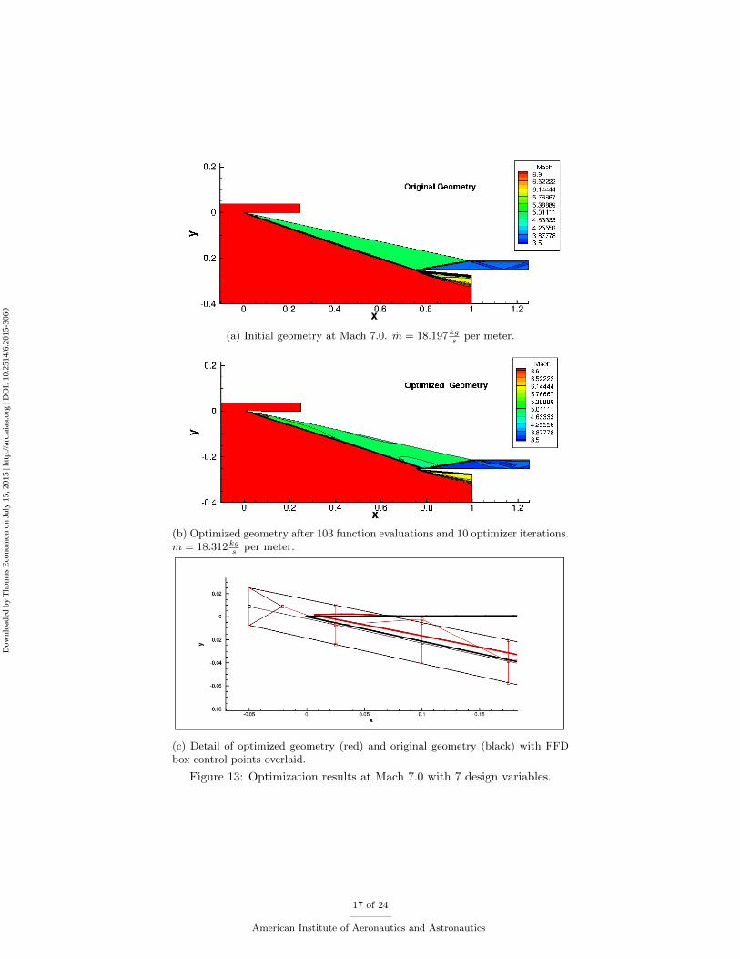
(a) Initial geometry at Mach 7.0. m = 18.197 kgs

per meter.

(b) Optimized geometry after 103 function evaluations and 10 optimizer iterations.m = 18.312 kg

sper meter.

(c) Detail of optimized geometry (red) and original geometry (black) with FFDbox control points overlaid.

Figure 13: Optimization results at Mach 7.0 with 7 design variables.

17 of 24


Dow

nloa

ded

by T

hom

as E

cono

mon

on

July

15,

201

5 | h

ttp://

arc.

aiaa

.org

| D

OI:

10.

2514

/6.2

015-

3060

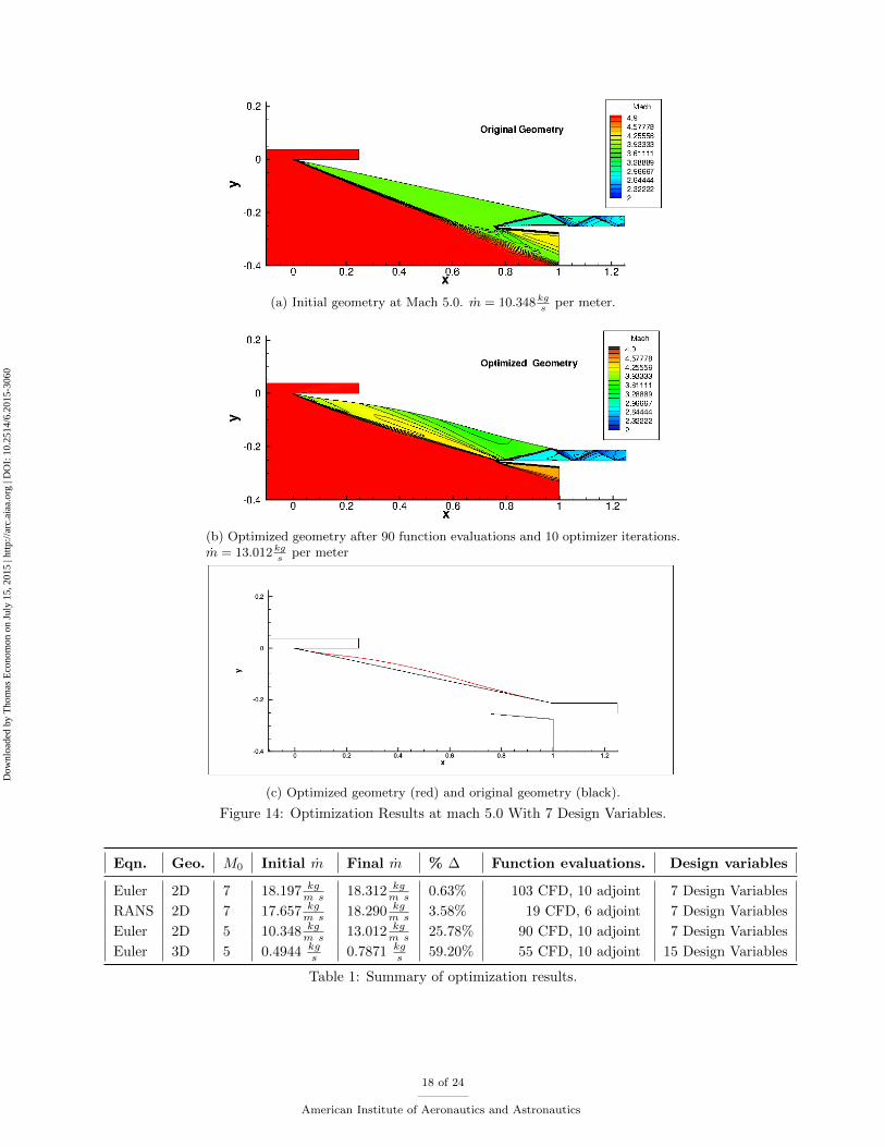
(a) Initial geometry at Mach 5.0. m = 10.348 kgs

per meter.


sper meter

(c) Optimized geometry (red) and original geometry (black).

Figure 14: Optimization Results at mach 5.0 With 7 Design Variables.

Eqn. Geo. M0 Initial m Final m % ∆ Function evaluations. Design variables

Euler 2D 7 18.197 kgm s 18.312 kg

m s 0.63% 103 CFD, 10 adjoint 7 Design Variables

RANS 2D 7 17.657 kgm s 18.290 kg


Euler 2D 5 10.348 kgm s 13.012 kg


Euler 3D 5 0.4944 kgs 0.7871 kg

s 59.20% 55 CFD, 10 adjoint 15 Design Variables

Table 1: Summary of optimization results.

18 of 24


Dow

nloa

ded

by T

hom

as E

cono

mon

on

July

15,

201

5 | h

ttp://

arc.

aiaa

.org

| D

OI:

10.

2514

/6.2

015-

3060

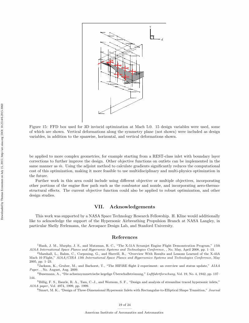
Figure 15: FFD box used for 3D inviscid optimization at Mach 5.0. 15 design variables were used, someof which are shown. Vertical deformations along the symmetry plane (not shown) were included as designvariables, in addition to the spanwise, horizontal, and vertical deformations shown.

be applied to more complex geometries, for example starting from a REST-class inlet with boundary layercorrections to further improve the design. Other objective functions on outlets can be implemented in thesame manner as m. Using the adjoint method to calculate gradients significantly reduces the computationalcost of this optimization, making it more feasible to use multidisciplinary and multi-physics optimization inthe future.

Further work in this area could include using different objective or multiple objectives, incorporatingother portions of the engine flow path such as the combustor and nozzle, and incorporating aero-thermo-structural effects. The current objective function could also be applied to robust optimization, and otherdesign studies.

VII. Acknowledgements

This work was supported by a NASA Space Technology Research Fellowship. H. Kline would additionallylike to acknowledge the support of the Hypersonic Airbreathing Propulsion Branch at NASA Langley, inparticular Shelly Ferlemann, the Aerospace Design Lab, and Stanford University.

References

1Hank, J. M., Murphy, J. S., and Mutzman, R. C., “The X-51A Scramjet Engine Flight Demonstration Program,” 15thAIAA International Space Planes and Hypersonic Systems and Technologies Conference, , No. May, April 2008, pp. 1–13.

2Marshall, L., Bahm, C., Corpening, G., and Sherrill, R., “Overview With Results and Lessons Learned of the X-43AMach 10 Flight,” AIAA/CIRA 13th International Space Planes and Hypersonics Systems and Technologies Conference, May2005, pp. 1–23.

3Jackson, K., Gruber, M., and Barhorst, T., “The HIFiRE flight 2 experiment: an overview and status update,” AIAAPaper , , No. August, Aug. 2009.

4Busemann, A., “Die achsensymmetrische kegelige Uberschallstromung,” Luftfahrtforschung, Vol. 19, No. 4, 1942, pp. 137–144.

5Billig, F. S., Baurle, R. A., Tam, C.-J., and Wornom, S. F., “Design and analysis of streamline traced hypersonic inlets,”AIAA paper , Vol. 4974, 1999, pp. 1999.

6Smart, M. K., “Design of Three-Dimensional Hypersonic Inlets with Rectangular-to-Elliptical Shape Transition,” Journal

19 of 24


Dow

nloa

ded

by T

hom

as E

cono

mon

on

July

15,

201

5 | h

ttp://

arc.

aiaa

.org

| D

OI:

10.

2514

/6.2

015-

3060

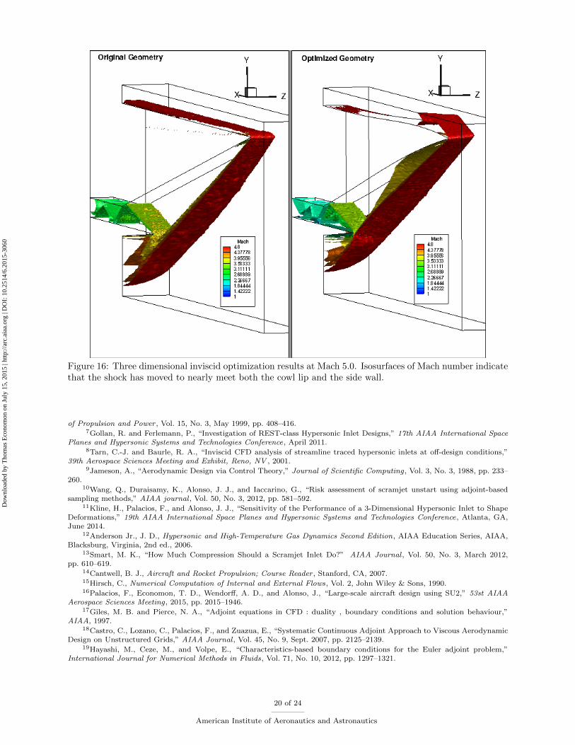
Figure 16: Three dimensional inviscid optimization results at Mach 5.0. Isosurfaces of Mach number indicatethat the shock has moved to nearly meet both the cowl lip and the side wall.

of Propulsion and Power , Vol. 15, No. 3, May 1999, pp. 408–416.7Gollan, R. and Ferlemann, P., “Investigation of REST-class Hypersonic Inlet Designs,” 17th AIAA International Space

Planes and Hypersonic Systems and Technologies Conference, April 2011.8Tarn, C.-J. and Baurle, R. A., “Inviscid CFD analysis of streamline traced hypersonic inlets at off-design conditions,”

39th Aerospace Sciences Meeting and Exhibit, Reno, NV , 2001.9Jameson, A., “Aerodynamic Design via Control Theory,” Journal of Scientific Computing, Vol. 3, No. 3, 1988, pp. 233–

260.10Wang, Q., Duraisamy, K., Alonso, J. J., and Iaccarino, G., “Risk assessment of scramjet unstart using adjoint-based

sampling methods,” AIAA journal , Vol. 50, No. 3, 2012, pp. 581–592.11Kline, H., Palacios, F., and Alonso, J. J., “Sensitivity of the Performance of a 3-Dimensional Hypersonic Inlet to Shape

Deformations,” 19th AIAA International Space Planes and Hypersonic Systems and Technologies Conference, Atlanta, GA,June 2014.

12Anderson Jr., J. D., Hypersonic and High-Temperature Gas Dynamics Second Edition, AIAA Education Series, AIAA,Blacksburg, Virginia, 2nd ed., 2006.

13Smart, M. K., “How Much Compression Should a Scramjet Inlet Do?” AIAA Journal , Vol. 50, No. 3, March 2012,pp. 610–619.

14Cantwell, B. J., Aircraft and Rocket Propulsion; Course Reader , Stanford, CA, 2007.15Hirsch, C., Numerical Computation of Internal and External Flows, Vol. 2, John Wiley & Sons, 1990.16Palacios, F., Economon, T. D., Wendorff, A. D., and Alonso, J., “Large-scale aircraft design using SU2,” 53st AIAA

Aerospace Sciences Meeting, 2015, pp. 2015–1946.17Giles, M. B. and Pierce, N. A., “Adjoint equations in CFD : duality , boundary conditions and solution behaviour,”

AIAA, 1997.18Castro, C., Lozano, C., Palacios, F., and Zuazua, E., “Systematic Continuous Adjoint Approach to Viscous Aerodynamic

Design on Unstructured Grids,” AIAA Journal , Vol. 45, No. 9, Sept. 2007, pp. 2125–2139.19Hayashi, M., Ceze, M., and Volpe, E., “Characteristics-based boundary conditions for the Euler adjoint problem,”

International Journal for Numerical Methods in Fluids, Vol. 71, No. 10, 2012, pp. 1297–1321.

20 of 24


Dow

nloa

ded

by T

hom

as E

cono

mon

on

July

15,

201

5 | h

ttp://

arc.

aiaa

.org

| D

OI:

10.

2514

/6.2

015-

3060

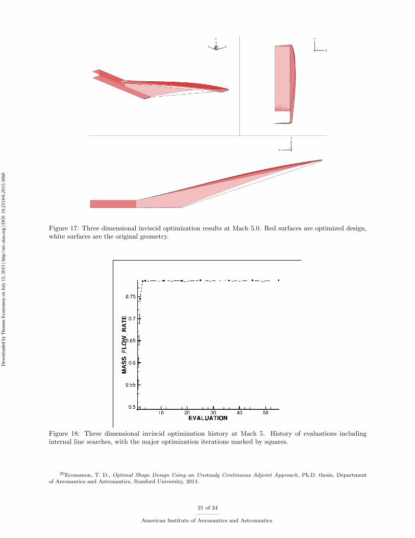
Figure 17: Three dimensional inviscid optimization results at Mach 5.0. Red surfaces are optimized design,white surfaces are the original geometry.

Figure 18: Three dimensional inviscid optimization history at Mach 5. History of evaluations includinginternal line searches, with the major optimization iterations marked by squares.

20Economon, T. D., Optimal Shape Design Using an Unsteady Continuous Adjoint Approach, Ph.D. thesis, Departmentof Aeronautics and Astronautics, Stanford University, 2014.

21 of 24


Dow

nloa

ded

by T

hom

as E

cono

mon

on

July

15,

201

5 | h

ttp://

arc.

aiaa

.org

| D

OI:

10.

2514

/6.2

015-

3060

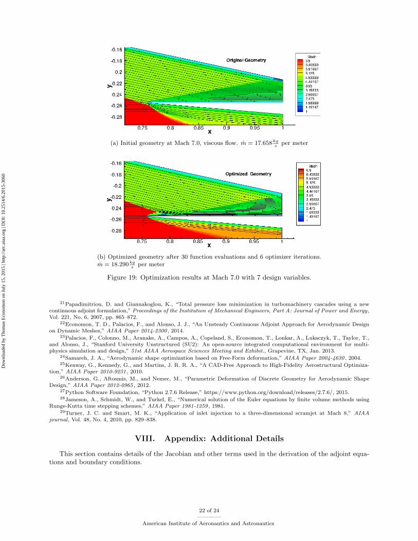
(a) Initial geometry at Mach 7.0, viscous flow. m = 17.658 kgs

per meter


sper meter

Figure 19: Optimization results at Mach 7.0 with 7 design variables.

21Papadimitriou, D. and Giannakoglou, K., “Total pressure loss minimization in turbomachinery cascades using a newcontinuous adjoint formulation,” Proceedings of the Institution of Mechanical Engineers, Part A: Journal of Power and Energy,Vol. 221, No. 6, 2007, pp. 865–872.

22Economon, T. D., Palacios, F., and Alonso, J. J., “An Unsteady Continuous Adjoint Approach for Aerodynamic Designon Dynamic Meshes,” AIAA Paper 2014-2300 , 2014.

23Palacios, F., Colonno, M., Aranake, A., Campos, A., Copeland, S., Economon, T., Lonkar, A., Lukaczyk, T., Taylor, T.,and Alonso, J., “Stanford University Unstructured (SU2): An open-source integrated computational environment for multi-physics simulation and design,” 51st AIAA Aerospace Sciences Meeting and Exhibit., Grapevine, TX, Jan. 2013.

24Samareh, J. A., “Aerodynamic shape optimization based on Free-Form deformation,” AIAA Paper 2004-4630 , 2004.25Kenway, G., Kennedy, G., and Martins, J. R. R. A., “A CAD-Free Approach to High-Fidelity Aerostructural Optimiza-

tion,” AIAA Paper 2010-9231 , 2010.26Anderson, G., Aftosmis, M., and Nemec, M., “Parametric Deformation of Discrete Geometry for Aerodynamic Shape

Design,” AIAA Paper 2012-0965 , 2012.27Python Software Foundation, “Python 2.7.6 Release,” https://www.python.org/download/releases/2.7.6/, 2015.28Jameson, A., Schmidt, W., and Turkel, E., “Numerical solution of the Euler equations by finite volume methods using

Runge-Kutta time stepping schemes,” AIAA Paper 1981-1259 , 1981.29Turner, J. C. and Smart, M. K., “Application of inlet injection to a three-dimensional scramjet at Mach 8,” AIAA

journal , Vol. 48, No. 4, 2010, pp. 829–838.

VIII. Appendix: Additional Details

This section contains details of the Jacobian and other terms used in the derivation of the adjoint equa-tions and boundary conditions.

22 of 24


Dow

nloa

ded

by T

hom

as E

cono

mon

on

July

15,

201

5 | h

ttp://

arc.

aiaa

.org

| D

OI:

10.

2514

/6.2

015-

3060

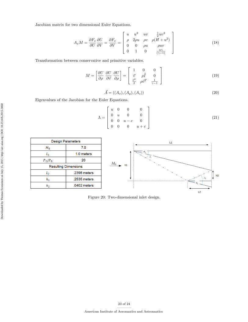
Jacobian matrix for two dimensional Euler Equations.

AxM =∂Fx∂U

∂U

∂V=∂Fx∂V

=

u u2 uv 1

2uv2

ρ 2ρu ρv ρ(H + u2)

0 0 ρu ρuv

0 1 0 uγ(γ−1)

(18)

Transformation between conservative and primitive variables.

M =

[∂U

∂ρ

∂U

∂~v

∂U

∂ρ

]=

1 0 0

~v ρ ¯I 0~v2

2 ρ~vT 1γ−1

(19)

~A = ((Ax), (Ay), (Az)) (20)

Eigenvalues of the Jacobian for the Euler Equations.

Λ =

u 0 0 0

0 u 0 0

0 0 u− c 0

0 0 0 u+ c

(21)

Figure 20: Two-dimensional inlet design.

23 of 24


Dow

nloa

ded

by T

hom

as E

cono

mon

on

July

15,

201

5 | h

ttp://

arc.

aiaa

.org

| D

OI:

10.

2514

/6.2

015-

3060

Figure 21: Unstructured mesh of 31,330 elements used for two-dimensional inviscid simulations.

Figure 22: Unstructured mesh of 1,120,620 elements used for two-dimensional viscous simulations. Cellspacing near walls such that y+ ≤ 1.0.

24 of 24


Dow

nloa

ded

by T

hom

as E

cono

mon

on

July

15,

201

5 | h

ttp://

arc.

aiaa

.org

| D

OI:

10.

2514

/6.2

015-

3060

Documents

Adjoint-Based Optimization of a Hypersonic Inlet · on the solid surface of a scramjet inlet to accelerate Monte-Carlo characterization of the probability of unstart. The contributions