Embed Size (px)
Citation preview

Contents
1 Measurement and Modeling of Wireless Channels. . . . . . . . . . . . . . . . 1David G. Michelson and Saeed S. Ghassemzadeh1.1 Introduction . . . . . . . . . . . . . . . . . . . . . . . . . . . . . . . . . . . .. . . . . . . . . . 11.2 A Brief History . . . . . . . . . . . . . . . . . . . . . . . . . . . . . . . . . . .. . . . . . . . 31.3 Characterization of Wireless Channels . . . . . . . . . . . . . .. . . . . . . . . . 51.4 Development of New Channel Models . . . . . . . . . . . . . . . . . . .. . . . . 91.5 Measurement of Wireless Channels . . . . . . . . . . . . . . . . . . .. . . . . . . 111.6 Recent Advances in Channel Modeling . . . . . . . . . . . . . . . . .. . . . . . 14
1.6.1 Channel Models for Ultrawideband Wireless Systems . .. 141.6.2 Channel Models for MIMO-based Wireless Systems . . . . 161.6.3 Channel Models for Body Area Networks . . . . . . . . . . . . . 191.6.4 Channel Models for Short-Range Vehicular Networks . .. 211.6.5 Channel Models for 60 GHz and Terahertz Systems . . . . . 23
1.7 Conclusions . . . . . . . . . . . . . . . . . . . . . . . . . . . . . . . . . . . . .. . . . . . . . . 25References . . . . . . . . . . . . . . . . . . . . . . . . . . . . . . . . . . . . . . . . .. . . . . . . . . . . . 25
2 OFDM: Principles and Challenges. . . . . . . . . . . . . . . . . . . . . . . . . . . . . 29Nicola Marchetti, Muhammad Imadur Rahman, Sanjay Kumar, RamjeePrasad2.1 Introduction . . . . . . . . . . . . . . . . . . . . . . . . . . . . . . . . . . . .. . . . . . . . . . 292.2 History and Development of OFDM . . . . . . . . . . . . . . . . . . . . .. . . . 302.3 The Benefit of Using Multi-carrier Transmission . . . . . . .. . . . . . . . 312.4 OFDM Transceiver Systems . . . . . . . . . . . . . . . . . . . . . . . . . .. . . . . . 342.5 Analytical model of OFDM System . . . . . . . . . . . . . . . . . . . . .. . . . . 35
2.5.1 Transmitter . . . . . . . . . . . . . . . . . . . . . . . . . . . . . . . . . . .. . . . 352.5.2 Channel . . . . . . . . . . . . . . . . . . . . . . . . . . . . . . . . . . . . . . .. . 372.5.3 Receiver . . . . . . . . . . . . . . . . . . . . . . . . . . . . . . . . . . . . . .. . . 382.5.4 Sampling . . . . . . . . . . . . . . . . . . . . . . . . . . . . . . . . . . . . . .. . 41
2.6 Advantages of OFDM System . . . . . . . . . . . . . . . . . . . . . . . . . .. . . . . 422.6.1 Combating ISI and Reducing ICI . . . . . . . . . . . . . . . . . . . .422.6.2 Spectral Efficiency . . . . . . . . . . . . . . . . . . . . . . . . . . . . .. . . 43
ix

x Contents
2.6.3 Some Other Benefits of OFDM System . . . . . . . . . . . . . . . 442.7 Disadvantages of OFDM System . . . . . . . . . . . . . . . . . . . . . . .. . . . . 45
2.7.1 Strict Synchronization Requirement . . . . . . . . . . . . . .. . . . 452.7.2 Peak-to-Average Power Ratio (PAPR) . . . . . . . . . . . . . . .. 462.7.3 Co-Channel Interference in Cellular OFDM . . . . . . . . . .. 46
2.8 OFDM System Design Issues . . . . . . . . . . . . . . . . . . . . . . . . . .. . . . . 462.8.1 OFDM System Design Requirements . . . . . . . . . . . . . . . . . 472.8.2 OFDM System Design Parameters . . . . . . . . . . . . . . . . . . . 48
2.9 Multi-carrier based Access Techniques . . . . . . . . . . . . . .. . . . . . . . . 492.9.1 Definition of Basic Schemes . . . . . . . . . . . . . . . . . . . . . . .. 49
2.10 Single-carrier vs Multi-carrier, TDE vs FDE . . . . . . . . .. . . . . . . . . . 532.10.1 Single Carrier FDE . . . . . . . . . . . . . . . . . . . . . . . . . . . . .. . . 532.10.2 Single-Carrier vs. Multi-Carrier, FDE vs. TDE . . . . .. . . . 542.10.3 Analogies and Differences between OFDM and SCFDE . 552.10.4 Interoperability of SCFDE and OFDM . . . . . . . . . . . . . . .. 57
2.11 OFDMA: An Example of Future Applications . . . . . . . . . . . .. . . . . 592.12 Conclusions . . . . . . . . . . . . . . . . . . . . . . . . . . . . . . . . . . . .. . . . . . . . . . 61References . . . . . . . . . . . . . . . . . . . . . . . . . . . . . . . . . . . . . . . . .. . . . . . . . . . . . 61
3 Recent Advances in Low-Correlation Sequences. . . . . . . . . . . . . . . . . . 65Gagan Garg, Tor Helleseth and P. Vijay Kumar3.1 Introduction . . . . . . . . . . . . . . . . . . . . . . . . . . . . . . . . . . . .. . . . . . . . . . 653.2 Cyclic Hadamard Difference Sets . . . . . . . . . . . . . . . . . . . .. . . . . . . . 66
3.2.1 Introduction . . . . . . . . . . . . . . . . . . . . . . . . . . . . . . . . . .. . . . 663.3 The Merit Factor of Binary Sequences . . . . . . . . . . . . . . . . .. . . . . . . 72
3.3.1 Introduction . . . . . . . . . . . . . . . . . . . . . . . . . . . . . . . . . .. . . . 723.4 Low correlation QAM sequences . . . . . . . . . . . . . . . . . . . . . .. . . . . . 78
3.4.1 Preliminaries . . . . . . . . . . . . . . . . . . . . . . . . . . . . . . . . .. . . . 793.4.2 Quaternary FamilyA . . . . . . . . . . . . . . . . . . . . . . . . . . . . . . 793.4.3 Canonical 16-QAM FamilyCQ . . . . . . . . . . . . . . . . . . . . . 803.4.4 Extensions and Improvements . . . . . . . . . . . . . . . . . . . . .. . 823.4.5 Example Generation of a 16-QAM Sequence . . . . . . . . . . 85
3.5 Low correlation zone sequences . . . . . . . . . . . . . . . . . . . . .. . . . . . . . 853.6 Additional Notes . . . . . . . . . . . . . . . . . . . . . . . . . . . . . . . . .. . . . . . . . . 88
3.6.1 Merit Factor . . . . . . . . . . . . . . . . . . . . . . . . . . . . . . . . . . .. . . 883.6.2 QAM Sequences . . . . . . . . . . . . . . . . . . . . . . . . . . . . . . . . . .893.6.3 Low Correlation Zone Sequences . . . . . . . . . . . . . . . . . . .. 89
3.7 Conclusions . . . . . . . . . . . . . . . . . . . . . . . . . . . . . . . . . . . . .. . . . . . . . . 89References . . . . . . . . . . . . . . . . . . . . . . . . . . . . . . . . . . . . . . . . .. . . . . . . . . . . . 90
4 Resource Allocation in Wireless Systems. . . . . . . . . . . . . . . . . . . . . . . 95Jon W. Mark and Lian Zhao4.1 Introduction . . . . . . . . . . . . . . . . . . . . . . . . . . . . . . . . . . . .. . . . . . . . . . 954.2 System Model . . . . . . . . . . . . . . . . . . . . . . . . . . . . . . . . . . . . .. . . . . . . 974.3 The Inverse ofΓS . . . . . . . . . . . . . . . . . . . . . . . . . . . . . . . . . . . . . . . . . 1014.4 Convergence of Power Distribution Law . . . . . . . . . . . . . . .. . . . . . . 102

Contents xi
4.4.1 With Zero Disturbance . . . . . . . . . . . . . . . . . . . . . . . . . . .. . 1024.4.2 With Nonzero Disturbance . . . . . . . . . . . . . . . . . . . . . . . .. . 1044.4.3 With Power Constraints . . . . . . . . . . . . . . . . . . . . . . . . . .. . 1054.4.4 Capacity Analysis . . . . . . . . . . . . . . . . . . . . . . . . . . . . . .. . . 107
4.5 Optimal Data Rate Allocation . . . . . . . . . . . . . . . . . . . . . . .. . . . . . . . 1084.5.1 Assumptions . . . . . . . . . . . . . . . . . . . . . . . . . . . . . . . . . . .. . 1084.5.2 Optimal Spreading Factor (OSF) Selection . . . . . . . . . .. . 1094.5.3 Rate Selection for GRP. . . . . . . . . . . . . . . . . . . . . . . . . . .. . 109
4.6 Joint Rate and Power Adaptation . . . . . . . . . . . . . . . . . . . . .. . . . . . . 1104.6.1 OSF-PC . . . . . . . . . . . . . . . . . . . . . . . . . . . . . . . . . . . . . . . .. 1104.6.2 GRP-PC . . . . . . . . . . . . . . . . . . . . . . . . . . . . . . . . . . . . . . . .. 111
4.7 Numerical Results . . . . . . . . . . . . . . . . . . . . . . . . . . . . . . . .. . . . . . . . . 1134.8 Conclusions . . . . . . . . . . . . . . . . . . . . . . . . . . . . . . . . . . . . .. . . . . . . . . 117References . . . . . . . . . . . . . . . . . . . . . . . . . . . . . . . . . . . . . . . . .. . . . . . . . . . . . 118
5 Iterative receivers and their graphical models. . . . . . . . . . . . . . . . . . . . 121Ezio Biglieri5.1 Introduction . . . . . . . . . . . . . . . . . . . . . . . . . . . . . . . . . . . .. . . . . . . . . . 1215.2 MAP symbol detection . . . . . . . . . . . . . . . . . . . . . . . . . . . . . .. . . . . . . 121
5.2.1 Factor graphs and the sum–product algorithm . . . . . . . .. . 1235.2.2 The basic factorization . . . . . . . . . . . . . . . . . . . . . . . . .. . . . 125
5.3 Channel and codes: A menagerie of factor graphs . . . . . . . .. . . . . . 1265.3.1 Modeling the channel . . . . . . . . . . . . . . . . . . . . . . . . . . . .. . 1265.3.2 Modeling the code . . . . . . . . . . . . . . . . . . . . . . . . . . . . . . .. . 128
5.4 Equalization . . . . . . . . . . . . . . . . . . . . . . . . . . . . . . . . . . . .. . . . . . . . . . 1305.5 Multiuser detection . . . . . . . . . . . . . . . . . . . . . . . . . . . . . .. . . . . . . . . . 1325.6 MIMO detection . . . . . . . . . . . . . . . . . . . . . . . . . . . . . . . . . . .. . . . . . . 1345.7 Multilevel coded modulation . . . . . . . . . . . . . . . . . . . . . . .. . . . . . . . . 1355.8 Convergence of the iterative algorithm . . . . . . . . . . . . . .. . . . . . . . . . 1375.9 Conclusions . . . . . . . . . . . . . . . . . . . . . . . . . . . . . . . . . . . . .. . . . . . . . . 137References . . . . . . . . . . . . . . . . . . . . . . . . . . . . . . . . . . . . . . . . .. . . . . . . . . . . . 138
6 Space-Time Codes: The Value of Correlation at the Transmitter . . . . 141Robert Calderbank, Songsri Sirianunpiboon and Stephen D. Howard6.1 Introduction . . . . . . . . . . . . . . . . . . . . . . . . . . . . . . . . . . . .. . . . . . . . . . 1416.2 Coding Gain and Diversity Gain . . . . . . . . . . . . . . . . . . . . . .. . . . . . . 1426.3 Space-Time Trellis Codes . . . . . . . . . . . . . . . . . . . . . . . . . .. . . . . . . . 1456.4 Space-Time Block Codes . . . . . . . . . . . . . . . . . . . . . . . . . . . .. . . . . . . 1476.5 Real and Complex Orthogonal Designs . . . . . . . . . . . . . . . . .. . . . . . 1496.6 Quasi-Orthogonal Space-Time Block Codes . . . . . . . . . . . .. . . . . . . 1536.7 Space-Time Codes that Simplify Receiver Signal Processing . . . . . 1556.8 Embedded Diversity . . . . . . . . . . . . . . . . . . . . . . . . . . . . . . .. . . . . . . . 1666.9 Multi-Level Space-Time Codes based on Binary Partitions of
QAM and PSK Constellations . . . . . . . . . . . . . . . . . . . . . . . . . . . .. . . 167References . . . . . . . . . . . . . . . . . . . . . . . . . . . . . . . . . . . . . . . . .. . . . . . . . . . . . 169
xii Contents
7 Fundamentals of Multi-User MIMO Communications . . . . . . . . . . . . 173Luca Sanguinetti and H. Vincent Poor7.1 Introduction . . . . . . . . . . . . . . . . . . . . . . . . . . . . . . . . . . . .. . . . . . . . . . 1737.2 System model . . . . . . . . . . . . . . . . . . . . . . . . . . . . . . . . . . . . .. . . . . . . 1747.3 Capacity . . . . . . . . . . . . . . . . . . . . . . . . . . . . . . . . . . . . . . . .. . . . . . . . . 176
7.3.1 Capacity Region of the Gaussian MIMO MAC . . . . . . . . . 1767.3.2 Gaussian MIMO Broadcast Channel . . . . . . . . . . . . . . . . . .184
7.4 Open- and closed-loop systems . . . . . . . . . . . . . . . . . . . . . .. . . . . . . . 1927.4.1 Open-loop systems . . . . . . . . . . . . . . . . . . . . . . . . . . . . . .. . 1937.4.2 Closed-loop systems . . . . . . . . . . . . . . . . . . . . . . . . . . . .. . . 194
7.5 System design . . . . . . . . . . . . . . . . . . . . . . . . . . . . . . . . . . . .. . . . . . . . 1947.5.1 Receiver design for uplink transmissions . . . . . . . . . .. . . . 1957.5.2 Transmitter design for downlink transmissions . . . . .. . . . 195
7.6 Limited feedback systems . . . . . . . . . . . . . . . . . . . . . . . . . .. . . . . . . . 2017.6.1 Channel quantization . . . . . . . . . . . . . . . . . . . . . . . . . . .. . . 2017.6.2 Random beamforming . . . . . . . . . . . . . . . . . . . . . . . . . . . . .2027.6.3 Transceiver optimization . . . . . . . . . . . . . . . . . . . . . . .. . . . 203
7.7 Conclusions . . . . . . . . . . . . . . . . . . . . . . . . . . . . . . . . . . . . .. . . . . . . . . 203References . . . . . . . . . . . . . . . . . . . . . . . . . . . . . . . . . . . . . . . . .. . . . . . . . . . . . 204
8 Collaborative Beamforming. . . . . . . . . . . . . . . . . . . . . . . . . . . . . . . . . . . 209Hideki Ochiai and Hideki Imai8.1 Introduction . . . . . . . . . . . . . . . . . . . . . . . . . . . . . . . . . . . .. . . . . . . . . . 2098.2 System Model and Beam Patterns of Fixed Nodes . . . . . . . . . .. . . . 211
8.2.1 Array Factor and Beam Pattern . . . . . . . . . . . . . . . . . . . . .. 2128.2.2 Beam Patterns of Linear Arrays . . . . . . . . . . . . . . . . . . . .. . 2148.2.3 Beam Patterns of Circular Arrays . . . . . . . . . . . . . . . . . .. . 217
8.3 Collaborative Beamforming by Randomly Distributed Nodes. . . . . 2198.3.1 Definition . . . . . . . . . . . . . . . . . . . . . . . . . . . . . . . . . . . . .. . . 2218.3.2 Average Beam Patterns . . . . . . . . . . . . . . . . . . . . . . . . . . .. . 2228.3.3 Distribution of Beam Patterns . . . . . . . . . . . . . . . . . . . .. . . 2248.3.4 Distribution of Maxima in Sidelobe . . . . . . . . . . . . . . . .. . 228
8.4 Conclusions . . . . . . . . . . . . . . . . . . . . . . . . . . . . . . . . . . . . .. . . . . . . . . 231References . . . . . . . . . . . . . . . . . . . . . . . . . . . . . . . . . . . . . . . . .. . . . . . . . . . . . 231
9 Cooperative Wireless Networks. . . . . . . . . . . . . . . . . . . . . . . . . . . . . . . . 233Behnaam Aazhang, Chris B. Steger, Gareth B. Middleton, and BrettKaufman9.1 Introduction . . . . . . . . . . . . . . . . . . . . . . . . . . . . . . . . . . . .. . . . . . . . . . 233
9.1.1 Overview . . . . . . . . . . . . . . . . . . . . . . . . . . . . . . . . . . . . . .. . 2339.1.2 Physical Layer Cooperation . . . . . . . . . . . . . . . . . . . . . .. . . 234
9.2 System Model . . . . . . . . . . . . . . . . . . . . . . . . . . . . . . . . . . . . .. . . . . . . 2369.2.1 Wide Area Network . . . . . . . . . . . . . . . . . . . . . . . . . . . . . . .2369.2.2 Multiple Flows and Flow Priority . . . . . . . . . . . . . . . . . .. . 2379.2.3 Cooperative Building Blocks . . . . . . . . . . . . . . . . . . . . .. . . 238
9.3 Learning about the Environment: Network State Information . . . . . 239
Contents xiii
9.3.1 NSI Overhead Management . . . . . . . . . . . . . . . . . . . . . . . . .2409.3.2 NSI Metric . . . . . . . . . . . . . . . . . . . . . . . . . . . . . . . . . . . . .. . 241
9.4 Finding the Optimal Cooperative Path . . . . . . . . . . . . . . . .. . . . . . . . 2419.4.1 Routing Cooperative Paths . . . . . . . . . . . . . . . . . . . . . . .. . . 2419.4.2 Trellis Representation . . . . . . . . . . . . . . . . . . . . . . . . .. . . . . 2429.4.3 Timing, Interference, and Duplexing Management . . . .. . 2439.4.4 Traversal Algorithms . . . . . . . . . . . . . . . . . . . . . . . . . . .. . . 244
9.5 Network Discovery . . . . . . . . . . . . . . . . . . . . . . . . . . . . . . . .. . . . . . . . 2459.5.1 Filling the Trellis: Gathering States, Edges, and NSI. . . . 2459.5.2 Filling the Trellis: Metanodes . . . . . . . . . . . . . . . . . . .. . . . 246
9.6 Conclusions . . . . . . . . . . . . . . . . . . . . . . . . . . . . . . . . . . . . .. . . . . . . . . 247References . . . . . . . . . . . . . . . . . . . . . . . . . . . . . . . . . . . . . . . . .. . . . . . . . . . . . 247
10 Interference Rejection and Management. . . . . . . . . . . . . . . . . . . . . . . . 251Arun Batra, James R. Zeidler, John G. Proakis, and Laurence B.Milstein10.1 Introduction . . . . . . . . . . . . . . . . . . . . . . . . . . . . . . . . . . .. . . . . . . . . . . 25110.2 Self-Interference Among Cooperating Systems . . . . . . .. . . . . . . . . 252
10.2.1 Interference Suppression to Enable Spectrum Sharing . . . 25210.2.2 Effects of Interference on Channel State Estimation. . . . . 254
10.3 Interference Mitigation in Block Modulated Multicarrier Systems . 25610.3.1 Interference Mitigation in an Uncoded Multicarrier
System . . . . . . . . . . . . . . . . . . . . . . . . . . . . . . . . . . . . . . . . . . 25910.3.2 Interference Mitigation in Coded Multicarrier Systems . . 26710.3.3 Doppler Sensitivity of OFDM in Mobile Applications .. . 269
10.4 Interference Suppression in Broadcast MIMO Systems . .. . . . . . . . 27110.4.1 Linear Precoding of the Transmitted Signals . . . . . . .. . . . 27210.4.2 Nonlinear Precoding of the Transmitted Signals: The
QR Decomposition . . . . . . . . . . . . . . . . . . . . . . . . . . . . . . . . 27410.4.3 Vector Precoding . . . . . . . . . . . . . . . . . . . . . . . . . . . . . .. . . . 27810.4.4 Lattice Reduction Method for Precoding . . . . . . . . . . .. . . 281
10.5 Conclusions . . . . . . . . . . . . . . . . . . . . . . . . . . . . . . . . . . . .. . . . . . . . . . 282References . . . . . . . . . . . . . . . . . . . . . . . . . . . . . . . . . . . . . . . . .. . . . . . . . . . . . 282
11 Cognitive Radio: From Theory to Practical Network Engineering . . . 287Ekram Hossain, Long Le, Natasha Devroye, and Mai Vu11.1 Introduction . . . . . . . . . . . . . . . . . . . . . . . . . . . . . . . . . . .. . . . . . . . . . . 28711.2 Information Theoretic Limits of Cognitive Networks . .. . . . . . . . . . 289
11.2.1 Cognitive Behavior: Interference Avoidance, Control,and Mitigation . . . . . . . . . . . . . . . . . . . . . . . . . . . . . . . . . . . . 289
11.2.2 Information Theoretic Basics . . . . . . . . . . . . . . . . . . .. . . . . 29011.2.3 Interference Avoidance: Spectrum Interweave . . . . .. . . . . 29111.2.4 Interference Control: Spectrum Underlay . . . . . . . . .. . . . . 29211.2.5 Interference Mitigation: Spectrum Overlay . . . . . . .. . . . . 295
11.3 Cognitive Sensing with Side-information . . . . . . . . . . .. . . . . . . . . . 30011.4 Interference Analysis . . . . . . . . . . . . . . . . . . . . . . . . . . .. . . . . . . . . . . 301

xiv Contents
11.4.1 A Network with Beacons . . . . . . . . . . . . . . . . . . . . . . . . . .. 30311.4.2 A Network with Primary Exclusive Regions . . . . . . . . . .. 304
11.5 Practical Cognitive Network Engineering: Interference ControlApproach . . . . . . . . . . . . . . . . . . . . . . . . . . . . . . . . . . . . . . . . . . .. . . . . 30611.5.1 Single-Antenna Case . . . . . . . . . . . . . . . . . . . . . . . . . . .. . . . 30611.5.2 Multiple Antenna Case . . . . . . . . . . . . . . . . . . . . . . . . . .. . . 308
11.6 Practical Cognitive Network Engineering: InterferenceAvoidance Approach . . . . . . . . . . . . . . . . . . . . . . . . . . . . . . . . . .. . . . 31011.6.1 Single-hop Case . . . . . . . . . . . . . . . . . . . . . . . . . . . . . . .. . . . 31011.6.2 Multi-hop Case . . . . . . . . . . . . . . . . . . . . . . . . . . . . . . . .. . . 318
11.7 Conclusions . . . . . . . . . . . . . . . . . . . . . . . . . . . . . . . . . . . .. . . . . . . . . . 319References . . . . . . . . . . . . . . . . . . . . . . . . . . . . . . . . . . . . . . . . .. . . . . . . . . . . . 320
12 Coded Bidirectional Relaying in Wireless Networks. . . . . . . . . . . . . . . 327Petar Popovski and Toshiaki Koike-Akino12.1 Introduction . . . . . . . . . . . . . . . . . . . . . . . . . . . . . . . . . . .. . . . . . . . . . . 32712.2 Preliminaries . . . . . . . . . . . . . . . . . . . . . . . . . . . . . . . . . .. . . . . . . . . . . 32912.3 Two–way Relaying with Decoding at the Relay . . . . . . . . . .. . . . . . 331
12.3.1 The Uplink Phase . . . . . . . . . . . . . . . . . . . . . . . . . . . . . . .. . 33112.3.2 The Broadcast Phase . . . . . . . . . . . . . . . . . . . . . . . . . . . .. . . 33212.3.3 Improved Broadcast Strategies . . . . . . . . . . . . . . . . . .. . . . 33312.3.4 Numerical Illustration . . . . . . . . . . . . . . . . . . . . . . . .. . . . . . 337
12.4 Two–way Relaying without Decoding at the Relay . . . . . . .. . . . . . 33812.4.1 Amplify–and–Forward (AF) . . . . . . . . . . . . . . . . . . . . . .. . 33812.4.2 Denoise–and–Forward (DNF) . . . . . . . . . . . . . . . . . . . . .. . 34012.4.3 Compress–and–Forward (CF) . . . . . . . . . . . . . . . . . . . . .. . 34112.4.4 Numerical Illustration and Variations . . . . . . . . . . .. . . . . . 343
12.5 Achieving the Two–Way Rates with Structured Codes. . . .. . . . . . . 34412.5.1 Parity–Check Codes for Binary Symmetric Channels . .. . 34412.5.2 Gaussian Channel . . . . . . . . . . . . . . . . . . . . . . . . . . . . . .. . . 345
12.6 Signalling Constellations for Finite Packet Lengths .. . . . . . . . . . . . 34812.6.1 XOR Denoising . . . . . . . . . . . . . . . . . . . . . . . . . . . . . . . . .. . 34912.6.2 Adaptive Denoising with Quintary Cardinality . . . . .. . . . 35012.6.3 End–to–End Throughput Performance . . . . . . . . . . . . . .. . 350
12.7 Conclusions . . . . . . . . . . . . . . . . . . . . . . . . . . . . . . . . . . . .. . . . . . . . . . 351References . . . . . . . . . . . . . . . . . . . . . . . . . . . . . . . . . . . . . . . . .. . . . . . . . . . . . 352
13 Minimum-cost Subgraph Algorithms for Static and DynamicMulticasts with Network Coding . . . . . . . . . . . . . . . . . . . . . . . . . . . . . . . 355Fang Zhao, Muriel Medard, Desmond Lun, and Asuman Ozdaglar13.1 Introduction . . . . . . . . . . . . . . . . . . . . . . . . . . . . . . . . . . .. . . . . . . . . . . 35513.2 Problem Formulation . . . . . . . . . . . . . . . . . . . . . . . . . . . . .. . . . . . . . . 358
13.2.1 Wireline Networks . . . . . . . . . . . . . . . . . . . . . . . . . . . . .. . . 35813.2.2 Wireless Networks . . . . . . . . . . . . . . . . . . . . . . . . . . . . .. . . 360
13.3 Decentralized Min-cost Subgraph Algorithms for Static Multicast . 362

Contents xv
13.3.1 Subgradient Method for Decentralized SubgraphOptimization . . . . . . . . . . . . . . . . . . . . . . . . . . . . . . . . . . . . . 363
13.3.2 Convergence Rate Analysis . . . . . . . . . . . . . . . . . . . . . .. . . 36613.3.3 Initialization and Primal Solution Recovery . . . . . .. . . . . . 37113.3.4 Simulation Results . . . . . . . . . . . . . . . . . . . . . . . . . . . .. . . . 373
13.4 Min-cost Subgraph Algorithms for Dynamic Multicasts .. . . . . . . . 37713.4.1 Nonrearrangeable Algorithm . . . . . . . . . . . . . . . . . . . .. . . . 37713.4.2 Rearrangeable Algorithms . . . . . . . . . . . . . . . . . . . . . .. . . . 38013.4.3 Simulation Results . . . . . . . . . . . . . . . . . . . . . . . . . . . .. . . . 383
13.5 Conclusions . . . . . . . . . . . . . . . . . . . . . . . . . . . . . . . . . . . .. . . . . . . . . . 385References . . . . . . . . . . . . . . . . . . . . . . . . . . . . . . . . . . . . . . . . .. . . . . . . . . . . . 386
14 Ultra Mobile Broadband (UMB) . . . . . . . . . . . . . . . . . . . . . . . . . . . . . . . 389Masoud Olfat14.1 Introduction . . . . . . . . . . . . . . . . . . . . . . . . . . . . . . . . . . .. . . . . . . . . . . 38914.2 UMB Overall Architecture . . . . . . . . . . . . . . . . . . . . . . . . .. . . . . . . . 39014.3 UMB Physical Layer . . . . . . . . . . . . . . . . . . . . . . . . . . . . . . .. . . . . . . 393
14.3.1 Superframe Structure . . . . . . . . . . . . . . . . . . . . . . . . . .. . . . 39314.3.2 UMB FL Channelization . . . . . . . . . . . . . . . . . . . . . . . . . .. 39814.3.3 Reverse Link in UMB . . . . . . . . . . . . . . . . . . . . . . . . . . . . .. 404
14.4 UMB MAC Layer . . . . . . . . . . . . . . . . . . . . . . . . . . . . . . . . . . . .. . . . . 41014.5 Other PHY/MAC layer features in UMB . . . . . . . . . . . . . . . . .. . . . . 42014.6 Conclusions . . . . . . . . . . . . . . . . . . . . . . . . . . . . . . . . . . . .. . . . . . . . . . 422References . . . . . . . . . . . . . . . . . . . . . . . . . . . . . . . . . . . . . . . . .. . . . . . . . . . . . 422
15 Mobile WiMAX . . . . . . . . . . . . . . . . . . . . . . . . . . . . . . . . . . . . . . . . . . . . . 425Masoud Olfat15.1 Introduction . . . . . . . . . . . . . . . . . . . . . . . . . . . . . . . . . . .. . . . . . . . . . . 42515.2 Standardization Process . . . . . . . . . . . . . . . . . . . . . . . . .. . . . . . . . . . . 42615.3 WiMAX Network Architecture . . . . . . . . . . . . . . . . . . . . . . .. . . . . . . 429
15.3.1 Network Reference Models . . . . . . . . . . . . . . . . . . . . . . .. . 43115.3.2 ASN profiles . . . . . . . . . . . . . . . . . . . . . . . . . . . . . . . . . . .. . 43115.3.3 Mobility Management . . . . . . . . . . . . . . . . . . . . . . . . . . .. . . 433
15.4 Physical Layer . . . . . . . . . . . . . . . . . . . . . . . . . . . . . . . . . .. . . . . . . . . . 43515.4.1 S-OFDMA Frame Structure . . . . . . . . . . . . . . . . . . . . . . . .. 43715.4.2 Subchannel Permutation . . . . . . . . . . . . . . . . . . . . . . . .. . . . 43915.4.3 Frame Structure . . . . . . . . . . . . . . . . . . . . . . . . . . . . . . .. . . . 44315.4.4 Channel coding . . . . . . . . . . . . . . . . . . . . . . . . . . . . . . . .. . . 44515.4.5 Multiple Antenna modes in Mobile WiMAX . . . . . . . . . . . 44515.4.6 Power control & Link Adaptation . . . . . . . . . . . . . . . . . .. . 450
15.5 Medium Access Control Layer . . . . . . . . . . . . . . . . . . . . . . .. . . . . . . 45315.5.1 Quality of Service . . . . . . . . . . . . . . . . . . . . . . . . . . . . .. . . . 45715.5.2 Power Saving Mode . . . . . . . . . . . . . . . . . . . . . . . . . . . . . .. 45815.5.3 Multicast Broadcast Services . . . . . . . . . . . . . . . . . . .. . . . . 45915.5.4 Handoff . . . . . . . . . . . . . . . . . . . . . . . . . . . . . . . . . . . . . .. . . 46015.5.5 Security and Authentication in WiMAX . . . . . . . . . . . . .. . 461
xvi Contents
15.6 WiMAX Performance . . . . . . . . . . . . . . . . . . . . . . . . . . . . . . .. . . . . . 46315.7 Future Work toward IMT-Advanced . . . . . . . . . . . . . . . . . . .. . . . . . . 464
15.7.1 Conclusions . . . . . . . . . . . . . . . . . . . . . . . . . . . . . . . . . .. . . . 465References . . . . . . . . . . . . . . . . . . . . . . . . . . . . . . . . . . . . . . . . .. . . . . . . . . . . . 466
16 An Overview of 3GPP Long-Term Evolution Radio Access Network . 469Sassan Ahmadi16.1 Introduction . . . . . . . . . . . . . . . . . . . . . . . . . . . . . . . . . . .. . . . . . . . . . . 469
16.1.1 Chronology of 3GPP Air-Interface TechnologyDevelopment . . . . . . . . . . . . . . . . . . . . . . . . . . . . . . . . . . . . . 470
16.1.2 3GPP LTE System Requirements . . . . . . . . . . . . . . . . . . . .47016.2 Overall Network Architecture . . . . . . . . . . . . . . . . . . . . .. . . . . . . . . . 47216.3 LTE Protocol Structure . . . . . . . . . . . . . . . . . . . . . . . . . . .. . . . . . . . . . 47416.4 Overview of the LTE Physical Layer . . . . . . . . . . . . . . . . . .. . . . . . . 475
16.4.1 Multiple Access Schemes . . . . . . . . . . . . . . . . . . . . . . . .. . . 47616.4.2 Operating Frequencies and Bandwidths . . . . . . . . . . . .. . . 47716.4.3 Frame Structure . . . . . . . . . . . . . . . . . . . . . . . . . . . . . . .. . . . 48016.4.4 Physical Resource Blocks. . . . . . . . . . . . . . . . . . . . . . .. . . . 48216.4.5 Modulation and Coding . . . . . . . . . . . . . . . . . . . . . . . . . .. . 48216.4.6 Physical Channel Processing . . . . . . . . . . . . . . . . . . . .. . . . 48316.4.7 Reference Signals . . . . . . . . . . . . . . . . . . . . . . . . . . . . .. . . . 48516.4.8 Physical Control Channels . . . . . . . . . . . . . . . . . . . . . .. . . . 48616.4.9 Physical Random Access Channel . . . . . . . . . . . . . . . . . .. . 48916.4.10 Cell Search . . . . . . . . . . . . . . . . . . . . . . . . . . . . . . . . . .. . . . . 49016.4.11 Link Adaptation . . . . . . . . . . . . . . . . . . . . . . . . . . . . . .. . . . . 49116.4.12 Multi-Antenna Techniques in LTE . . . . . . . . . . . . . . . .. . . 491
16.5 Overview of the LTE Layer 2 . . . . . . . . . . . . . . . . . . . . . . . . .. . . . . . 49216.5.1 Logical and Transport Channels . . . . . . . . . . . . . . . . . .. . . 49416.5.2 ARQ and HARQ in LTE. . . . . . . . . . . . . . . . . . . . . . . . . . . . 49616.5.3 Packet Data Convergence Sublayer (PDCP) . . . . . . . . . .. . 497
16.6 Radio Resource Control Functions (RRC) . . . . . . . . . . . . .. . . . . . . . 49716.7 Mobility Management and Handover in LTE . . . . . . . . . . . . .. . . . . 49816.8 LTE Performance . . . . . . . . . . . . . . . . . . . . . . . . . . . . . . . . .. . . . . . . . 49916.9 Future Work toward IMT-Advanced . . . . . . . . . . . . . . . . . . .. . . . . . . 50116.10 Conclusions . . . . . . . . . . . . . . . . . . . . . . . . . . . . . . . . . . .. . . . . . . . . . . 502References . . . . . . . . . . . . . . . . . . . . . . . . . . . . . . . . . . . . . . . . .. . . . . . . . . . . . 503
Index . . . . . . . . . . . . . . . . . . . . . . . . . . . . . . . . . . . . . . . . . . . . . . . . . . .. . . . . . . . . . 505

Chapter 7Fundamentals of Multi-User MIMOCommunications
Luca Sanguinetti and H. Vincent Poor
7.1 Introduction
In recent years, the remarkable promise of multiple-antenna techniques has mo-tivated an intense research activity devoted to characterizing the theoretical andpractical issues associated with multiple-input multiple-output wireless channels.This activity was first focused primarily on single-user communications but morerecently there has been extensive work on multi-user settings. The aim of this chap-ter is to provide an overview of the fundamental information-theoretic results andpractical implementation issues of multi-user multiple-antenna networks operatingunder various conditions of channel state information.
The contents of this chapter are as follows. In Section 1 we introduce basic nota-tion and describe the system model of interest. The latter includes both uplink anddownlink models for a general mobile communication system operating with mul-tiple antennas at both the base station and mobile terminals. In Section 2 we con-centrate on channel capacity as a means of characterizing such systems, and reviewbasic results under various operating conditions, including patterns of knowledgeof information about the state of the channel between transmitter(s) and receiver(s).In Section 3 we address the problem of acquisition of channelstate informationat the transmitter and receiver, and describe the distinctive features of open-loopand closed-loop systems. In Section 4 we provide an overviewof system designissues and discuss techniques that require channel state information at the transmit-ter, while in Section 5 we briefly review some recent work on techniques that allow
Luca SanguinettiDipartimento di Ingegneria dell’Informazione, Universita di Pisa, Via Caruso 16, Pisa 56122, Italye-mail:[email protected]
H. Vincent PoorDepartment of Electrical Engineering, Princeton University, Olden Street, Princeton, NJ 08544,USA e-mail:[email protected]
173

174 Luca Sanguinetti and H. Vincent Poor
achievement of the potential benefits of multiple antennas using limited feedbacklinks. Finally, we draw some conclusions in Section 6.
Due to the considerable amount of work in this field, this exposition is necessarilyincomplete, and rather reflects the subjective taste and inclination of the authors. Tocompensate for this partial view, a list of references is included as an entree into theextensive literature available on the subject.
7.2 System model
We consider both the uplink and downlink of a flat-fading multi-user multiple-inputmultiple-output (MIMO) network1 in which the base station (BS) is endowed withM antennas, andK mobile terminals (MTs) are simultaneously active. Withoutlossof generality, we assume that all the MTs are equipped with the same numberN ofantennas2.
We denote byHul,k ∈ CM×N theuplink channel matrix whose entries representthe channel gains from the transmit antennas at thekth MT to the receive antennasof the BS and are modeled as independent complex circularly symmetric Gaussianrandom variable with zero-mean and unit variance3. Moreover, we assume that theusers are randomly located within the cell so as to experience independent fadingchannels. Such a model is known in the literature as independent and identicallydistributed (i.i.d) Rayleigh fading (see for example the tutorial paper of Biglierietal. in [4] for a detailed discussion of other channel models). Atthe BS, the discrete-time received signaly ∈ CM×1 can be written as
y =K
∑k=1
Hul,kxk +n (7.1)
wherexk ∈ CN×1 is the signal transmitted by thekth user whilen ∈ CM×1 is the re-ceiver noise modeled as a complex Gaussian vector with zero-mean and covariance
1 Although specific for a flat-fading channel, the model adopted throughout the chapter can easilybe extended to frequency selective environments using orthogonal frequency-division multiplexing(OFDM) as a transmission technique.2 We adopt the following notation: boldface upper and lower-case letters denote matrices andvectors. We useA = diag{a(n) ; n= 1,2, . . . ,N} to indicate anN×N diagonal matrix with entriesa(n) andB = diag{B(1),B(2), . . . ,B(Q)} to represent a block diagonal matrix. We use respectivelyA−1, tr{A} and|A| to denote the inverse, trace and determinant of a matrixA. We denote byIK
and0K the identity and null matrices of orderK, respectively, while we use E{·} for expectation,‖·‖ for the Euclidean norm of the enclosed vector and the superscripts ∗, T and H for complexconjugation, transposition and Hermitian transposition,respectively. The notationA ≥ 0 indicatesthatA is positive semidefinite while[·]k,ℓ denote the (k, ℓ)th entry of the enclosed matrix. Finally,we use conv{·} for the convex hull operator.3 This model can be reasonably adopted whenever the transmit and receive antennas operate ina nonline-of-sight rich scattering environment and the antenna spacing is larger than the spatialcoherence distance.

7 Fundamentals of Multi-User MIMO Communications 175
matrix IM. We denote byXk = E{xkxHk } the transmit covariance matrix of thekth
MT and assume that it is constrained to satisfy the followinginequality
tr(Xk) ≤ ρk (7.2)
whereρk is the power available for transmission at thekth MT. Letting Hul =[Hul,1Hul,2 · · ·Hul,K ], we may rewrite (7.1) in matrix notation as
y = Hulx+n (7.3)
where we have definedx = [xT1 ,xT
2 , . . . ,xTK ]T .
Similarly, we denote byHdl,k ∈CN×M thedownlinkchannel matrix whose( j, i)thentry now represents the channel gain from theith transmit antenna at the BS tothe jth receive antenna of thekth MT and again is modeled as a complex circu-larly symmetric Gaussian random variable with zero-mean and unit variance. Thediscrete-time signal at thekth MT can be written as
r k = Hdl,ks+zk (7.4)
wheres∈ CM×1 is the signal transmitted by the BS whilezk ∈ CN×1 accounts forthe receiver noise modeled as a complex Gaussian vector withzero-mean and co-variance matrixIN. We denote byS= E{ssH} the transmit covariance matrix andassume that the BS is subject to the following power constraint
tr(S) ≤ p. (7.5)
Collecting the signals received at all MTs into a single vector r ∈ CKN×1 yields
r = Hdls+z (7.6)
whereHdl = [HTdl,1HT
dl,2 · · · HTdl,K ]T while z = [zT
1 ,zT2 , . . . ,zT
K ]T is Gaussian withzero mean and covariance matrixIKN.
The systems described by (7.3) and (7.6) are respectively known in the technicalliterature as the Gaussian MIMO multiple-access-channel (MAC) and the GaussianMIMO broadcast channel (BC), respectively. They essentially represent an exten-sion of the single antenna uplink and downlink systems first formally introducedby Ahslwede [1] and Cover [14] in the early 1970s. Since then they have attracteda great deal of attention in the research community as they well model the com-munication links of a large variety of practical systems such as cellular networks,wireless local area networks (WLANs) and digital subscriber line (DSL) links (toname only a few).

176 Luca Sanguinetti and H. Vincent Poor
7.3 Capacity
In the sequel, we consider the capacity of the two multi-userMIMO networks de-scribed above. Although not the only way of characterizing these channels, the ca-pacity is without doubt the most important information-theoretic measure that drivesthe design of communication systems. In a single-user system, it is operationally de-fined as the maximum data rate that the channel can support with an arbitrarily lowerror probability while it is mathematically computed maximizing the mutual in-formationI(x,y) between the inputx and the outputy of the channel over all thepossible choices ofPx the distribution ofx, i.e.,
C = maxPx
I(x,y). (7.7)
On the other hand, a multi-user channel withK users is characterized by aK-dimensional capacity regionC ∈ RK
+ (we denote byRK+ the set ofK-tuples with
non-negative real-valued entries). Each point is this region is identified by aK-tupleR = (R1,R2, . . . ,RK) and represents a combination of rates at which users can sendinformation with an arbitrarily low error probability.
7.3.1 Capacity Region of the Gaussian MIMO MAC
We begin by reviewing the basic results on the channel capacity of the GaussianMIMO MAC (MIMO GMAC) described by (7.2) and (7.3). In particular, we con-sider two different situations. The first is referred to as thedeterministic channelandrelies on the assumption thatHul is constant and known at the receiver and transmit-ters. The second, known asfading channel, is the case in whichHul is time-varyingandergodic[4]. We also assume that in this latter case the transmittersare subjectto short-term power constraints meaning that each MT must meet the constraint in(7.2) for every channel realization. This is equivalent to saying that the availablepower cannot be adaptively allocated over time. Moreover, we will consider thesituation in which the channel is either known or not at the MTs. For notationalsimplicity, in this section we drop the subscriptul.
7.3.1.1 Deterministic channel
To ease understanding, we begin by considering a two-user scenario (i.e.,K = 2).Moreover, we assume that each user user is equipped with a single transmit antenna(i.e.,N = 1). In this case the capacity region is a pentagon in the positive quadrantof the(R1,R2)−plane which can be written as follows [15]

7 Fundamentals of Multi-User MIMO Communications 177
. .
.
.
R1 + R2 ! log IM + "1h1h1H+ "2h2h2
H
R2 ! log IM + "2h2h2H
R1 ! log IM + "1h1h1H
R1
R2
A B
C
D
Fig. 7.1 Example of the capacity region in a two user scenario with single transmit antennas.
CMAC(H,ρ) =
R ∈ R2+ :
0≤ R1 ≤ log∣
∣IM + ρ1h1hH1
∣
∣
0≤ R2 ≤ log∣
∣IM + ρ2h2hH2
∣
∣
R1 +R2 ≤ log∣
∣IM + ρ1h1hH1 + ρ2h2hH
2
∣
∣
(7.8)
whereρ = [ρ1,ρ2] while hk ∈ CM×1 (k = 1,2) represents thekth column of theuplink channel matrix, i.e.,H = [h1,h2]. The above equation leads to an interest-ing physical interpretation. The achievable rate of each user cannot exceed that ofa single-user system in which the other user is turned off. This is made evident bythe first two terms on the right-hand-side (RHS) of (7.8). On the other hand, thelast term on the RHS of (7.8) indicates that the sum rate cannot be larger than thatof a system in which the two active users act as a single user equipped with twotransmit antennas sending independent signals and subjectto different power con-straints [15].
An example of the capacity region for a two-user scenario is depicted in Fig. 1.The point A corresponds to the maximum rate at which user 1 canreliably sendinformation over the channel when user 2 is not transmitting. The corner point Dis the complementary rate for user 2. The points B and C are of particular interestbecause they represent the maximum achievable sum rate given by
RmaxMAC = max
(R1,R2) ∈ CMAC(H,ρ)R1 +R2 (7.9)
and they can be achieved by resorting to a two-stageinterference cancellation(known also assuccessive decoding) scheme, which operates as follows. In the firststage, it detects the data stream of user 1 treating the signal from user 2 as interfer-ence. In the second stage, the contribution of user 1 is reconstructed and cancelledout from the received signal before detection of user 2. Based on the above proce-dure, it can be easily found that the maximum rate at which user 1 can transmit isgiven by

178 Luca Sanguinetti and H. Vincent Poor
R1 = log(
1+ ρ1hH1
(
IM + ρ2h2hH2
)−1h1
)
(7.10)
where ρ1hH1
(
IM + ρ2h2hH2
)−1h1 represents the signal-to-noise-plus-interferenceratio (SINR) for user 1 when user 2 is treated as colored Gaussian noise [49]. Onthe other hand, the maximum rate at which user 2 can transmit is given by
R2 = log(
1+ ρ2hH2 h2
)
. (7.11)
The t-uple (R1,R2) of (7.10) and (7.11) is precisely the point B in Fig. 1. The corre-sponding sum rate can be easily computed as follows. We beginby using the identity(1+BA)= |IM +AB| with A = ρ1
(
IM + ρ2h2hH2
)−1h1 andB = hH1 so as to rewrite
(7.10) as follows
R1 = log∣
∣
∣IM + ρ1
(
IM + ρ2h2hH2
)−1h1hH
1
∣
∣
∣(7.12)
or, equivalently,
R1 = log∣
∣IM + ρ1h1hH1 + ρ2h2hH
2
∣
∣− log∣
∣IM + ρ2h2hH2
∣
∣ . (7.13)
Similarly, (7.11) becomes
R2 = log∣
∣IM + ρ2h2hH2
∣
∣ . (7.14)
Collecting all the above results togheter, it follows that
R1 +R2 =∣
∣IM + ρ1h1hH1 + ρ2h2hH
2
∣
∣ (7.15)
which is exactly the maximum sum rate as depicted in Fig. 1. Clearly, inverting thecancellation order allows one to achieve the other corner point C. Any other pointon the segment BC guarantees the same maximum achievable sumrate and canbe attained by means oftime-sharingbetween the two different strategies at pointsB and C or by using an alternative technique known asrate-splittingproposed byRimoldi and Urbanke in [40].
WhenN > 1, each MT has more degrees of freedom that can be used to improvethe system performance. To see how this comes about, we decompose the covariancematrices asXk = UkDkUH
k (k = 1,2) whereUk is unitary (i.e.,UkUHk = I ) andDk
is a diagonal matrix whose entries represent the power allocated to the differentdata streams and have to satisfy the following inequality tr(Dk)≤ ρk (obtained from(7.2) after substitutingXk with UkDkUH
k ). Thus, it follows that whenN > 1 eachMT can arbitrarily choose between different power allocations and rotations beforesending the data streams out of the transmit antennas. This is in contrast to the caseof N = 1 where each MT has no other choice than allocating all the available powerto the single transmit data stream. In general, different strategies result into differentpairs(X1,X2) so that the capacity region is a convex set given by the union of aninfinite number of rate regions, each corresponding to a different pair(X1,X2) and
7 Fundamentals of Multi-User MIMO Communications 179
R1
R2
B
C
A
D
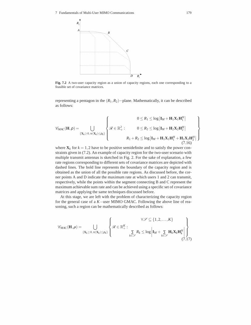
Fig. 7.2 A two-user capacity region as a union of capacity regions, each one corresponding to afeasible set of covariance matrices.
representing a pentagon in the(R1,R2)−plane. Mathematically, it can be describedas follows:
CMAC(H,ρ)=⋃
{Xk≥0, tr(Xk)≤ρk}
R ∈ R2+ :
0≤ R1 ≤ log∣
∣IM +H1X1HH1
∣
∣
0≤ R2 ≤ log∣
∣IM +H2X2HH2
∣
∣
R1 +R2 ≤ log∣
∣IM +H1X1HH1 +H2X2HH
2
∣
∣
(7.16)whereXk for k = 1,2 have to be positive semidefinite and to satisfy the power con-straints given in (7.2). An example of capacity region for the two-user scenario withmultiple transmit antennas is sketched in Fig. 2. For the sake of explanation, a fewrate regions corresponding to different sets of covariancematrices are depicted withdashed lines. The bold line represents the boundary of the capacity region and isobtained as the union of all the possible rate regions. As discussed before, the cor-ner points A and D indicate the maximum rate at which users 1 and 2 can transmit,respectively, while the points within the segment connecting B and C represent themaximum achievable sum rate and can be achieved using a specific set of covariancematrices and applying the same techniques discussed before.
At this stage, we are left with the problem of characterizingthe capacity regionfor the general case of aK−user MIMO GMAC. Following the above line of rea-soning, such a region can be mathematically described as follows:
CMAC(H,ρ) =⋃
{Xk≥0, tr(Xk)≤ρk}
R ∈ RK+ :
∀S ⊆ {1,2, . . . ,K}
∑k∈S
Rk ≤ log
∣
∣
∣
∣
IM + ∑k∈S
HkXkHHk
∣
∣
∣
∣
(7.17)

180 Luca Sanguinetti and H. Vincent Poor
whereρ is now given byρ = [ρ1,ρ2, . . . ,ρK ] while S refers to an arbitrary subsetof {1,2, . . . ,K}. Each set of covariance matrices results in aK−dimensionalpoly-matroidof achievable rates as shown by Tse and Hanly in [48], i.e.,
R ∈ RK+ :
∀S ⊆ {1,2, . . . ,K}
∑k∈S
Rk ≤ log
∣
∣
∣
∣
IM + ∑k∈S
HkXkHHk
∣
∣
∣
∣
(7.18)
while the capacity region corresponds to the union of such polymatroids over allsets of covariance matrices. An interesting problem is how to design the set{Xk}that achieve any point on the boundary of the capacity region. This problem can beaddressed as follows. We begin by observing that(7.17) is a convex set and, thus,its boundary points can be achieved by maximizing a linear combination of the userrates [7]:
µ1R1 + µ2R2 + . . .+ µKRK (7.19)
whereµk are non-negative real-valued parameters satisfyingµ1+µ2+ . . .+µK = 1.Theµk’s are known asuser prioritiesdue to the fact that for a given set of covariancematrices and user priorities, the corner points of the corresponding polymatroid areattained using successive decoding in order ofincreasing priority, i.e., the user withthe highest priority is decoded last. Assume for example that µ1 ≤ µ2 ≤ . . .≤ µK . Inthis case the signal of userk is decoded before any other user with priorityµi > µk
so that its achievable rate is given by
Rk = log
∣
∣
∣
∣
∣
∣
IM +
(
IM +K
∑i=k+1
H iX iHHi
)−1
HkXkHHk
∣
∣
∣
∣
∣
∣
(7.20)
where(IM + ∑Ki=k+1H iX iHH
i )−1 denotes the covariance matrix of userk when usersµi > µk are treated as colored Gaussian noise. Using simple mathematical deriva-tions, the above equation can be rewritten as follows
Rk = log
∣
∣
∣
∣
∣
IM +K
∑i=k
HkXkHHk
∣
∣
∣
∣
∣
− log
∣
∣
∣
∣
∣
IM +K
∑i=k+1
HkXkHHk
∣
∣
∣
∣
∣
. (7.21)
Substituting (7.21) into (7.19), it follows that the optimal set {Xk} maximizing(7.19) can be found by solving the following problem [12]
maxX
f ({µk})
subject to Xk ≥ 0 and tr{Xk} ≤ ρk for k = 1,2, . . . ,K
(7.22)
whereX = diag{X1,X2, . . . ,XK} and f ({µk}) is given by

7 Fundamentals of Multi-User MIMO Communications 181
f ({µk}) = µ1 log
∣
∣
∣
∣
∣
IM +K
∑k=1
HkXkHHk
∣
∣
∣
∣
∣
+K
∑k=2
(µk− µk−1) log
∣
∣
∣
∣
∣
IM +K
∑i=k
H iX iHHi
∣
∣
∣
∣
∣
.
(7.23)Finding the exact solution of (7.22) is in general a computationally expensive task.However, we observe that we are maximizing a linear combination of concave func-tions subject to constraints that are convex in the set of positive semidefinite ma-trices [50]. Hence, the problem is convex and the solution can be efficiently foundusing numerical optimization tools [7].
When the objective is to maximize the sum rate of the system (i.e., µ1 = µ2 =. . . = µK), we may rewrite (7.22) as
RmaxMAC = max
{Xk≥0, tr(Xk)≤ρk ∀k}log
∣
∣
∣
∣
∣
IM +K
∑k=1
HkXkHHk
∣
∣
∣
∣
∣
(7.24)
and the solution can be found by using the following generalization of the single-user water-filling algorithm as shown by Yuet al. in [65]:
Multi-user iterative water-filling algorithm
1) Initialization
a) SetXk = 0N for k = 1,2, . . . ,K
2) Until the sum rate converges
a) Until k < K
i) ComputeX′ = IM + ∑ j 6=k H jX jHHj
ii) SetXk = argmaxX
log(
HkXHHk +X′
)
As seen, the optimal{Xk} is computed iteratively and at each iteration the covari-ance matrix of one user is given by the single-user water-filling solution obtainedby treating the others as Gaussian noise. In [65], the authors show that the aboveprocedure converges to the maximum sum rate solution irrespective to the startingpoint. All this can be formally characterized by the following theorem.
Theorem 7.1.(Yu et al. (2004))In a K-user MIMO GMAC,Xk is an optimal so-lution to the sum rate maximization problem if, and only if,Xk is the single-userwaterfilling solution covariance matrix of the channel withmatrix Hk and with co-variance matrixIM +∑K
i=1,i 6=k H iX iHHi of the Gaussian noise, for all k= 1,2, . . . ,K.
7.3.1.2 Fading Channel
We begin by considering the case of perfect channel knowledge at both the trans-mitters and receiver and then focus on the situation in whichonly the receiver hasthis information. In the former case, Yuet al. in [63] show that the system underinvestigation can be thought of as a set ofparallel non-interferingMIMO GMACs.

182 Luca Sanguinetti and H. Vincent Poor
In particular, each element of the set corresponds to a different channel realization.The ergodic capacity4 region is thus computed as an average of the capacity regionscharacterizing the parallel MIMO GMACs. Mathematically, we have that
CMAC(ρ) = EH {CMAC(H,ρ)} (7.25)
whereCMAC(H,ρ) is given in (7.17) while the statistical expectation must becom-puted with respect to the channel distribution. Similarly to the deterministic channel,we concentrate on the ergodic sum rate and aim at computing the optimal set of co-variance matrices. This is tantamount to solving
RmaxMAC = EH
{
max{Xk≥0, tr(Xk)≤ρk ∀k}
log
∣
∣
∣
∣
∣
IM +K
∑k=1
HkXkHHk
∣
∣
∣
∣
∣
}
. (7.26)
As discussed by Rhee and Cioffi in [63], the above problem is convex and its so-lution can be computed by resorting to an extension of the iterative water-fillingalgorithm (described previously) which operates independently for each channel re-alization. On the other hand, when channel state information (CSI) is available onlyat the receiver, the MTs cannot adapt their covariance matrices to the specific chan-nel realization so that they are forced to use the same transmission strategy over allfading states. In this case, the ergodic capacity region is still computed as an averageof the capacity regions corresponding to the different channel realizations but nowwith a given transmission strategy. Mathematically, we have that
CMAC(ρ)=⋃
{Xk≥0, tr(Xk)≤ρk ∀k}
R ∈ RK+ :
∀S ⊆ {1,2, . . . ,K}
∑k∈S
Rk ≤ EH
{
log
∣
∣
∣
∣
IM + ∑k∈S
HkXkHHk
∣
∣
∣
∣
}
(7.27)which is equivalent to (7.17) except for the statistical expectation. Then, its bound-ary and optimal set{Xk} can be computed via the maximization problem given in(7.22) even though the computation of the statistical expectation makes the problema bit more challenging. However, in the particular case of independent and identi-cally distributed (i.i.d.) Rayleigh channels, this optimization is no longer required asthe boundary of the capacity region can be achieved by means of Gaussian codes andthe same uniform power allocation strategy over all fading states. This is formalizedin the following theorem (see for example [46] and [39]).
Theorem 7.2.For an i.i.d. Rayleigh channel, the ergodic capacity regionof a K-user MIMO GMAC is a polymatroid given by
4 The ergodic capacity is the direct extension of capacity to fading channels. It corresponds to themaximum mutual information averaged over all channel realizations. However, there are a numberof different ways to define the capacity of fading channels [4].

7 Fundamentals of Multi-User MIMO Communications 183
CMAC(ρ) =
R ∈ RK+ :
∀S ⊆ {1,2, . . . ,K}
∑k∈S
Rk ≤ EH
{
log
∣
∣
∣
∣
IM + ∑k∈S
ρkN HkHH
k
∣
∣
∣
∣
}
(7.28)
and any point on its boundary is achieved when each user uses aGaussian code anda uniform power allocation strategy.
Based on the above result, it follows that in these circumstances the maximum er-godic sum rate takes the form
RmaxMAC = EH
{
log
∣
∣
∣
∣
∣
IM +K
∑k=1
ρk
NHkH
Hk
∣
∣
∣
∣
∣
}
. (7.29)
7.3.1.3 Asymptotic analysis
In the following, we are interested in evaluating how the sumrate of a MIMOGMAC scales with respect to some system parameters such as the number oftransmit and receive antennas, the number of users and the signal-to-noise ratios(SNRs)5. To this end, we consider the fading channel and focus on the case whereCSI is available only at the receiver. Assuming that the sameamount of power isallocated to the different users, i.e.,ρk = ρ/K, from (7.29) we have
RmaxMAC = EH
{
log∣
∣
∣IM +
ρKN
HHH∣
∣
∣
}
. (7.30)
Interestingly, the RHS of the above equation is equivalent to the ergodic capacityof a single-user MIMO system equipped withKN transmit andM receive antennaswhen only the receiver has channel knowledge [46]. This means that in these cir-cumstances the lack of cooperation between the MTs does not reduce the capacitywhich is exactly the same of a fully cooperative system. Hence, we may concludethat in an i.i.d. Rayleigh fading model where all users have the same power con-straint CSI at the receiver is enough to achieve the potential benefits of a fully coop-erative multiple antenna system. Similarly to a single-user MIMO system, channelknowledge at the transmitters leads to an improvement of theperformance in thelow SNR regime but becomes irrelevant when the SNR increasesas illustrated byViswanathet al. in [54]. The authors show also that such an information providesvanishing advantages even in a system in which the SNR is fixedbut the number oftransmit antennas and the number of users is taken to infinity. These results allowus to characterize the asymptotic performance of a MIMO GMACon the basis of(7.30)6:
5 As the noise power is normalized to one, the SNRs coincide with the transmit powers.6 We stress again the fact that most of the results reported in this chapter depend heavily on i.i.dRayleigh fading. Different models such as spatially correlated fading, Ricean fading and so forthmay lead to different conclusions. A good survey of the results obtained on these subjects can befound in [22] .
184 Luca Sanguinetti and H. Vincent Poor
1. If M is fixed andKN→∞, the law of large numbers yields1KN HHH → IM (almostsurely) so that (7.30) tends to an upper bound given by
RmaxMAC = log|IM + ρ IM| = log(1+ ρ)M = M log(1+ ρ) (7.31)
from which it follows that asymptotically (inKN) the sum rate grows linearlywith M. This is equivalent to saying that a 3 dB increase in the SNR gives aM(bit/s/Hz) increase in the sum rate. As increasingKN is essentially equivalentto increasing the number of independent paths, this is a simple example of thefact that fading is a resource to beexploitedrather than a detrimental effect to bemitigated [55].
2. According to [39], in the high-SNR regime and for any finitevalues ofM, K andN the ergodic sum rate in (7.30) is well-approximated by
RmaxMAC = min(M,KN) log(1+ ρ)+o(1) (7.32)
whereo(1) denotes a term not increasing withρ . From the above equation itfollows that
A∞MAC = lim
ρ→∞
RmaxMAC
logρ= min(M,KN) (7.33)
which is commonly called themultiplexing gainand essentially measures thedegrees of freedomavailable for reliable communication [21].
A close inspection of (7.33) leads to the following interesting practical observation.IncreasingK while keepingN fixed makes the sum rate grow linearly withM as longasKN ≥ M. This is in sharp contrast to a single-user MIMO system in which themultiplexing gain would be constant and bounded by min(M,N). From a practicalpoint of view, this is very interesting as increasing the number of antennas at theBS is not an issue of concern as it is at the MTs. Moreover, we observe that thissituation is even more realistic thanKN ≤ M as many networks already operatewith a number of users that is much larger that the number of transmit antennas.
7.3.2 Gaussian MIMO Broadcast Channel
The capacity region of a general BC is still unknown. Up to now, only an achievablerate region computed by Marton in [35] is available, but it isnot clear whether itcoincides or not with the capacity region. On the other hand,for those BCs (knownasdegraded) in which the active users can be essentially ordered from the strongestto the weakest the capacity region is a well-known result andcan be achieved using atechnique known assuperposition codingdiscussed by Bergman in [3] and outlinedas follows. At the transmitter, the signal is obtained as a linear combination of thedifferent data streams and is decoded at the receivers usingsuccessive cancellation
7 Fundamentals of Multi-User MIMO Communications 185
in order of increasing order, i.e., each user decodes and removes from the receivedsignal all the weaker user contributions before decoding its own signals.
The single antenna Gaussian BC (GBC) (i.e.,M = N = 1) belongs to the classof degraded BCs as the users can be naturally ordered according to their respectiveSINRs. In the two user case (assuming without loss of generality |h1| > |h2|), thecapacity region can be described as follows [15]:
CBC(H, p)=⋃
{p1,p2}:p1+p2=p
R ∈ R2+ :
R1 ≤ log(
1+ |h1|2 p1
)
R2 ≤ log
(
1+ |h2|2 p2
(
1+ |h2|2 p1
)−1)
(7.34)whereH = [h1,h2]
T while p1 andp2 denote the powers allocated to users 1 and 2,respectively, and must satisfy the equalityp1 + p2 = p.
Although the MIMO GBC does not fall within the class of degraded BC chan-nels7, its capacity region has recently been computed by Weingartenet al. in [60].Such a result is probably one of the major achievements in information theory of therecent years as it establishes that there exists a non-degraded BC whose capacity re-gion can be fully characterized. In the following, we first consider the deterministicchannel model and overview the fundamental steps that have led to the computationof the capacity region in this scenario. Then, we concentrate on the fading modeland summarize some of the more important asymptotic results. To simplify notation,in the sequel we drop the subscriptdl.
7.3.2.1 Deterministic channel
In the next, we begin by introducing two basic concepts that have driven the researchactivity in this area over the last years, namely, dirty paper coding (DPC) and uplink-downlink duality. Then, we illustrate how they has been employed to compute theachievable sum rate of a MIMO-GBC. Finally, we give a short description of themain result stated in [60].
Dirty paper coding
DPC is a channel coding technique closely related to superposition coding in whichthe user data streams are encoded sequentially in such a way that at the receive sideeach user sees no interference from the others that have beenpreviously encoded. Tohighlight the effectiveness of a DPC-based strategy in the downlink of a multi-userscenario, we again consider the two-user single-antenna GBC. As for superposition
7 Roughly speaking, the main reason is that the different propagation channels in a MIMO BC aredescribed by matrices and no natural ordering exists for matrices.

186 Luca Sanguinetti and H. Vincent Poor
coding, we assume that the transmit signal is computed as a linear combination ofthe user data streams and denote bypk (k = 1,2) the power allocated to thekthuser. The data stream for user 2 is encoded using Gaussian coding while DPC isused to encode that for user 1 treating user 2 as non-casuallyknown interference(this is equivalent to saying that the received signal at user 1 is not affected by thecontribution of user 2).
At this stage, in order to compute the achievable rates of DPCwe make use ofa surprising result known aswriting on dirty paperwhich was presented by Costain [16].
Theorem 7.3.(Costa, 1983)Consider any channel whose output signal y takes thisform y= x+ i + w where i and w are independent Gaussian random variables. Ifiis known non-casually at the transmitter and not at the receiver then the capacity ofthe channel is the same as if i were not present. Moreover, thecapacity-achieving xis statistically independent of i.
Based on the above theorem, the achievable rate of user 1 is given by
R1 = log(
1+ |h1|2 p1
)
(7.35)
and it is equivalent to the capacity of a system in which user 2is not present. On theother hand, user 2 decodes its data stream treating user 1 as Gaussian interferenceso that its achievable rate takes the form
R2 = log
(
1+ |h2|2 p2
(
1+ |h2|2 p1
)−1)
. (7.36)
The t-uple(R1,R2) is precisely a point on the boundary of the capacity region givenin (7.34) which is known to be achievable using superposition coding and succes-sive cancellation. Thus, it follows that the above DPC-based transmission techniquerepresents an alternative capacity-achieving solution for the single-antenna GBC.
We now turn to the general case described by (7.6) and extend the above tech-nique according to a result of Yuet al. in [64] which essentially generalizes theorem3 to the vector case. Specifically, the transmit signal is given byx = ∑K
k=1xk wherethekth streamxk is Gaussian with covariance matrixSk = E{xkxH
k } and it is encodedaccording to DPC so as to remove the interference of the streams with indicesi < k.The transmit covariance matrix takes the formS = ∑K
k=1Sk (the user signals areuncorellated by construction [16]) and the power constraint in (7.5) becomes
K
∑k=1
tr(Sk) ≤ p. (7.37)
According to [64] for a given user orderingπ = [π(1),π(2), . . . ,π(K)]T and a givenset{Sπ(k)} satisfying (7.37), the following rates are achievable

7 Fundamentals of Multi-User MIMO Communications 187
Rπ(k) = log
∣
∣
∣
∣
Hπ(k)
K∑i=k
Sπ(i)HHπ(k) + IN
∣
∣
∣
∣
∣
∣
∣
∣
Hπ(k)
K∑
i=k+1Sπ(i)HH
π(k) + IN
∣
∣
∣
∣
k = 1,2, . . . ,K (7.38)
whereπ(i) denotes theith user to be encoded. The DPC rate region is given by theconvex hull of the union of the above t-uples over all possible sets of permutationsand covariance matrices satisfying (7.37). Thus, we have
RDPC(H, p) = conv
⋃
{π}
⋃
{Sk}:∑Kk=1 tr(Sk)≤ p
{
(Rπ(1),Rπ(2), . . . ,Rπ(K)) ∈ RK+
}
.
(7.39)It is worth observing that the rates given in (7.38) are neither a concave nor a con-vex function of the correlation matrices. This makes the computation of the DPCregion given in (7.39) a very computationally demanding task as the optimal set ofcovariance matrices can be found only by means of an exhaustive search.
Uplink-downlink duality
Theuplink-downlink dualityhas been observed in seemingly different contexts andforms in the literature. It was first pointed out by Telatar in[46] where it is shownthat for a single user MIMO system interchanging the transmitter and receiver doesnot change the capacity of the system. On the other hand, Jindalet al.in [27] demon-strate that the capacity region of the single-antenna GBC isequal to the capacityregion of thedual (i.e., hul,k = h∗dl,k ∀k) Gaussian MAC subject to the samesumpower constraint instead of the common individual constraints. The general MIMOGBC has been later investigated by Viswanath, P. and Tse in [56] and Vishwanath,S.et al. in [57] and their major results can be formalized as follows.
Theorem 7.4.(Viswanath, P., and Tse (2003) and Vishwanath, S.et al.(2003))TheDPC rate region of the MIMO GBC given in (7.6) subject to a power constraint pis equivalent to
RDPC(H, p) = CD−MAC(H, p) (7.40)
whereCD−MAC(H, p) is the capacity region of the dual MIMO GMAC:
CD−MAC(H, p)=⋃
{Xk≥0}:∑Kk=1 tr(Xk)≤p
R ∈ RK+ :
∀S ⊆ {1,2, . . . ,K}
∑k∈S
Rk ≤ log
∣
∣
∣
∣
IM + ∑k∈S
HHk XkHk
∣
∣
∣
∣
.
(7.41)
188 Luca Sanguinetti and H. Vincent Poor
A close observation of (7.41) indicates thatCD−MAC is equal to (7.17) after replacingHk with HH
k and imposing a sum power constraintp. This is not only extremelyinteresting from an information-theoretic point of view but it is also very appealingfor practical purposes. In fact, it provides a powerful toolto numerically evaluate theDPC rate region. This is due to the fact that in contrast to (7.39) the boundary of thedual MAC capacity region (as discussed in Section 2.1.1) canbe easily computedby solving a convex problem. Each corner point can then be attained by using thecorresponding optimal set of covariance matrices{Xk} and resorting to successivedecoding with a specific order. A possible example of the DPC rate region is shownin [22] (Fig. 9).
The question, though, is now how to achieve the same data rates in the downlink.The answer is provided by Vishwanath, S.et al. in [57] where the authors proposea computationally efficient transformation that takes as inputs the optimal uplinkset{Xk} and the corresponding decoding order and returns as outputsthe set ofdownlink matrices{Sk} satisfying
∑Kk=1 tr(Xk) = ∑K
k=1 tr(Sk) (7.42)
and achieving the same data rates by means of DPC in the reverse order.
Achievable sum rate
The pioneering work in the computation of the capacity region of a MIMO GBCis due to Caire and Shamai [8]. Therein, the authors considerthe simple case of asystem with two users (K = 2) each equipped with a single receive antenna (N = 1)and compute through direct calculation the maximum sum rateof DPC. Then, itsoptimality is proved making use of the Sato upper bound [41] which refers to thecapacity of a system where the users are allowed to cooperate.
The above result has been later extended to the general case (K > 2 and/orN > 1)by several authors simultaneously. In particular, Yuet al.in [66] compute the achiev-able sum rate of the system as the saddle-point of a Gaussian mutual informationgame, where a player chooses a transmit covariance matrix tomaximize the mu-tual informationI(x,y) and amalicious naturechooses a fictitious noise correlationmatrix to minimizeI(x,y). Once computed, this upper bound is used to prove thatthe structure of the optimal coding technique takes the formof DPC. Independentand different proofs of such a result are also given by Viswanath, P., and Tse [56]and Vishwanath, S.et al. [57]. Both essentially rely on theuplink-downlink dualityand, instead of proving directly the optimality of DPC aim atdemonstrating that themaximum sum rate of the dual MAC is equivalent to the Sato upper bound with thesame constraint on the transmit power.
All these results can be collected into the following theorem which represents afundamental step toward the computation of the entire capacity region.

7 Fundamentals of Multi-User MIMO Communications 189
Theorem 7.5.(Caire and Shamai (2003), Viswanath, P., and Tse (2003), Vish-wanath, S.et al. (2003) and Yuet al. (2004))The maximum sum rate of a MIMOGBC is achieved by means of DPC, i.e.,
RmaxBC = max
(R1,R2,...,RK)∈RDPC(H,p)R1 +R2+ . . .+RK. (7.43)
From the above theorem and using (7.38), it follows that the problem of computingthe maximum sum rate can be formulated as
maxπ
maxS
K∑
k=1log
∣
∣
∣
∣
Hπ(k)
K∑
i=kSπ(i)H
Hπ(k)+IN
∣
∣
∣
∣
∣
∣
∣
∣
Hπ(k)
K∑
i=k+1Sπ(i)H
Hπ(k)+IN
∣
∣
∣
∣
subject to Sk ≥ 0∀k and∑Kk=1 tr{Sk} ≤ p,
(7.44)
and its solution can be found by resorting to two efficient iterative algorithms pre-sented by Jindalet al. in [28]. Both rely on the uplink-downlink duality to reformu-late the problem into the following convex form:
RmaxBC = max
{Xk≥0}: ∑Kk=1 tr(Xk)≤p
log
∣
∣
∣
∣
∣
IM +K
∑k=1
HHk XkHk
∣
∣
∣
∣
∣
(7.45)
which is a subset of (7.41) and differs from (7.24) only in thesum power constraint.Hence, iterative algorithms inspired by the water-filling policy discussed in [65] canbe used to converge to the optimal set{Xk} which is then mapped to its correspond-ing dual{Sk} using the transformation discussed previously [57].
The capacity region
Up to now, we have seen that DPC is the optimal strategy to achieve the maximumsum rate of a MIMO GBC and also that its rate region coincides with the dualMIMO GMAC capacity region. Moreover, we have recalled that the capacity regionof the single-antenna GBC is equal to the capacity region of its dual GMAC [27].Collecting all these facts together, the most obvious idea that comes to mind is eitherto find a better achievable rate region that may not be attained through DPC or toprove that the DPC region is indeed the capacity region of theMIMO GBC. Therehave been many attempts in these directions but only Weingartenet al. in [60] havefinally provided an answer to these claims. In particular, itis found that the DPCregion isexactlythe capacity region of the MIMO GBC as stated in the followingtheorem.
Theorem 7.6.Weingartenet al. (2006))Let CBC(H, p) denote the capacity regionof the MIMO GBC given in (7.6) and subject to the power constraint p. Then
CBC(H, p) = RDPC(H, p). (7.46)

190 Luca Sanguinetti and H. Vincent Poor
This important result is achieved by making use of all the keyideas described thusfar plus several new concepts such asdegradedandenhancedMIMO BCs and anextension of Bergmans’ proof. Due to space limitations, we cannot provide furtherdetails about these results or their proofs; we invite the interested reader to referto [60].
7.3.2.2 Fading channel
When perfect CSI is available at both transmitter and receivers, the computation ofthe ergodic capacity region can be addressed following the same arguments as inSection 2.2.1. In fact, in this case similarly to the uplink,the system reduces to aset of parallel non-interfering MIMO GBCs each one corresponding to a differentchannel realization (see for example Yu and Rhee [69] and Yu [68]). Then, theergodic capacity region is given by
CBC(p) = CD−MAC(p) (7.47)
whereCD−MAC(p) is now computed from (7.25) using (7.17) after replacingHk
with HHk and imposing the sum power constraintp. Following the same arguments
as before, the computation of the ergodic sum rate can be formulated as follows
RmaxBC = EH
{
max{Xk≥0}: ∑K
k=1 tr(Xk)≤plog
∣
∣
∣
∣
∣
IM +K
∑k=1
HHk XkHk
∣
∣
∣
∣
∣
}
(7.48)
and the solution can be computed by resorting to the algorithms discussed in [28]and [57].
On the other hand, when CSI is not available at the BS, the ergodic capacityregion is still unknown as it is the optimal coding strategy,since DPC relies onperfect channel knowledge. However, there exists one special setting in which thisdoes not hold true: the case in which the user channels arestatisticallyequivalentand the same number of antennas is employed at all MTs (as the system investigatedhere) [2]. In fact, in these circumstances if we assume that any one of theK userscan reliably decode its received signal then the same can be done by any otheruser. Hence, the sum rate of the system is bounded by the capacity of the channelbetween the BS and any single MT. For the i.i.d. Rayleigh fading model, this can bemathematically formulated as
CBC(p) =
{
R ∈ RK+ :
K
∑k=1
Rk ≤ EH
{
log∣
∣
∣IM +
pM
H1HH1
∣
∣
∣
}
}
(7.49)
from which it follows that the optimal coding strategy in this case is time-divisionmultiple-access (TDMA), i.e., transmit to only one user at atime. Hence, the ergodicsum rate is given by

7 Fundamentals of Multi-User MIMO Communications 191
RmaxBC = EH
{
log
∣
∣
∣
∣
IM +PM
H1HH1
∣
∣
∣
∣
}
. (7.50)
The RHS of the above equation is equivalent to the ergodic capacity of a single usersystem withM transmit andN receive antennas. This implies that, as already pointedout by Caire and Shamai in [8] for the single receive antenna case, the complete lackof channel knowledge at the transmitter reduces the multiplexing gain of the systemto min(M,N). This observation has been extended to a generalisotropic 8 channelmodel by Jafar and Goldsmith in [26]. It is worth noting that such a result is insharp contrast to the uplink where the multiplexing gain is always the same as thatof a fully cooperative system, i.e, min(M,KN), independently from the CSI at thetransmitters. We elaborate further on this in the next subsection.
7.3.2.3 Asymptotic results
As was done for the MIMO GMAC, we now analyze how the sum rate ofthe MIMOGBC scales with the system parameters. In particular, we first focus on the case inwhich the transmitter and receivers both have perfect channel knowledge and thenconsider the situation in which only the receivers have thisinformation. When CSIis available at both BS and MTs, the following asymptotic results are in order.
1. If KN andp are fixed andM → ∞, the ergodic sum rate grows as [29]
RmaxBC = KN log
(
1+M
KNp
)
. (7.51)
This result can be easily proven as follows. From (7.48), themaximum achievablesum rate is obviously lower bounded by the sum rate achieved using a uniformpower allocation for each user and each fading state:
RmaxBC ≥ EH
{
log∣
∣
∣IKN +
pKN
HHH∣
∣
∣
}
. (7.52)
As M goes to infinity applying the law of large number yieldsHHH → MIKN
(almost surely) so that (7.51) easily follows from the RHS ofthe above equationusing the same arguments leading to (7.31). Moreover, such alower bound canbe shown to be tight whenM becomes large [32].
2. If M and p are fixed andK → ∞, then for anyN the ergodic sum rate growsas [43]
RmaxBC = M loglogKN. (7.53)
The intuition behind this result is that whenK grows and CSI is available atthe BS it is likely to findM channels to transmit over. On the other hand, thedoubly logarithmic increase withKN is essentially due to the inherentmulti-user
8 A set of channelsH is said to be isotropic if for each channel realizationHk ∈ H we have thatHkUk ∈ H whereUk is unitary [26].

192 Luca Sanguinetti and H. Vincent Poor
diversity. The latter can be thought of as a form ofselection diversityand it wasoriginally introduced by Knopp and Humblet in [24]. It is essentially based on thefollowing idea. As the users’ signals undergoindependenttime-varying fadingchannels, it is likely that at a given time there are users whose channels are notfaded. Intuitively, the maximization of the sum rate can be achieved by allocatingat any time the available resources to the ”best” set of users. As we select theseusers as the maximum amongKN possible choices in an i.i.d. Rayleigh fadingchannel, the effective SNR benefits by a factor logKN [43].
3. If M, K, andN are kept fixed, then the multiplexing gain is given by [29]
A∞BC = lim
ρ→∞
RmaxBC
logρ= min(M,KN) (7.54)
which is the same as that of a system in which the users are allowed to cooperate.
On the the other hand, when CSI is available only at the MTs thefollowing resultsapply:
1. If M, N andp are fixed, the ergodic sum rate does not increase asK → ∞, therebymeaning that
limK→∞
RmaxBC
loglogK= 0. (7.55)
This is due to the fact that the optimal strategy in these circumstances (as dis-cussed in Section 2.2.2) is to transmit to a randomly selected user during eachtransmission time-slot.
2. If M, K, andN are kept fixed, then the multiplexing gain is given by [29]
A∞BC = min(M,N) (7.56)
which is the same as that of a single-user system.
From the above results, it follows that CSI at the transmitter plays a key role fordownlink transmissions. This is in contrast to the uplink where CSI is not mandatoryto guarantee maximum capacity scaling.
7.4 Open- and closed-loop systems
As seen from the above discussion, in order to exploit the potential benefits of multi-ple antennas, explicit knowledge of the channel parametersis required at the receiverin the uplink and at both receivers and transmitter in the downlink.
Channel estimation at the receiver has received significantattention in the lit-erature and several different solutions are already available for both uplink anddownlink9. Common approaches are thetraining-aided schemes where a known
9 It is worth observing that channel estimation in uplink transmissions is a more demanding task.The main problem is that users transmit from different locations and the signals arrive at the BS

7 Fundamentals of Multi-User MIMO Communications 193
sequence of symbols calledpilots are periodically inserted within the transmittedsignal (see [47] and the references therein). Although easyto implement, the use ofpilot-based schemes inevitably reduces the spectral efficiency of the system. Thishas inspired considerable research on eitherblind or semi-blindchannel estimationtechniques, which are largely categorized into subspace-based or decision-directedmethods. Both solutions lead to a considerable saving in training overhead but in-crease the required computational burden. An excellent overview of the results ob-tained in this area can be found in [6] (chapters 14 and 17).
Channel acquisition at the transmitter is in general a more demanding task. Inthe sequel, we discuss two different operating techniques that have to be used on thebasis of the characteristics of the system under investigation.
7.4.1 Open-loop systems
This technique relies on the channel reciprocity between alternate uplink and down-link transmissions and, thus, it is suitable for time-division-duplex systems (suchas Hyperlan/2 and IEEE 802.11a) where the same frequency band is alternativelyused for transmission and reception. In particular, if the channel variations are suf-ficiently slow (as occurs in indoor applications) or the time-lag between two con-secutive time-slots is much smaller than the channel coherence time, the uplink anddownlink propagation channels can reasonably be considered to be reciprocal. Un-der this assumption, the transmitter can estimate the channel during the receptionphase and employ this estimate in the subsequent transmission time-slot. We referto this strategy asopen-loopsince CSI is acquired without requiring any feedbackinformation.
Despite its appealing features, the design of an open-loop system poses severaltechnical challenges that, if not properly addressed, may preclude the validity ofthe reciprocity principle. Apart from the channel estimation errors that may occurduring the reception phase, the main impairment is due to thefact that in practicalapplications channel estimation is usually performed at the baseband level after theradio-frequency (RF) chain. This calls for efficient calibration schemes able to com-pensate for any possible amplitude and phase error between the transmit and receiveRF chains. If not properly mitigated, these errors might result in severe degradationof the system performance [17]. From a practical point of view, however, this cali-bration is not easy to achieve and, thus, open-loop systems are nowadays consideredunsuitable for commercial multi-user systems.
after passing through different multipath channels. This means that the BS must estimate a largenumber of parameters in the presence of multiple access interference, which is inevitably expectedto degrade the accuracy of the channel estimates. On the other hand, in downlink transmissions, allthe signals arriving from the transmitter to a given terminal propagate through the same channel.This facilitates the channel estimation task, which can be accomplished with the same methodsemployed for single-user applications.
194 Luca Sanguinetti and H. Vincent Poor
An alternative solution to overcome these impairments is touse a form oflong-term reciprocityknown asstatistical reciprocity. The latter is intrinsically immuneto the aforementioned drawbacks as it relies on the fading distribution of the two-way communication channel rather than on its instantaneousrealization. In thoseapplications characterized by a strong correlation eitherin space or time, the fadingdistribution between uplink and downlink transmissions isusually the same andit can be employed to perform a kind of statistical adaptation at the transmitter.Unfortunately, although easier to implement, this approach comes at the price ofnon-negligible performance loss with respect to a system that uses instantaneouschannel knowledge.
7.4.2 Closed-loop systems
An effective way to overcome most of the drawbacks of open-loop systems consistsof performing the estimation process at the receiver and feeding channel measure-ments back to the transmitter through a reliable reverse link. This is a reasonablealternative since control channels are already used in systems such as 3G cellularnetworks to perform power control. We refer to this strategyasclosed-loopand ob-serve that it is generally suitable for those applications in which the reciprocity con-dition cannot be guaranteed or does not hold a priori. Among others, this is the caseof frequency-division-duplex systems (such as cellular networks), in which trans-mission and reception take place over different frequency bands whose separationis typically larger than the coherence bandwidth of the channel. Albeit intrinsicallyrobust to non-reciprocal effects, a closed-loop system presents the following majortechnical challenges. First, it suffers from an inherent feedback delay which mightresult in outdated CSI at the time of transmission. Second, the feedback channelmust be characterized by a high level of reliability, thereby making the link designtask much more challenging than in open-loop systems. Third, the amount of infor-mation exchanged increases linearly with the total number of channel propagationpaths, i.e.,M×KN, and counts against the overall spectral efficiency of the system.
7.5 System design
In this section, we provide an overview of system design issues in multi-user MIMOsystems. We focus on the downlink for which transmitter design is the key issuewhile we touch on the uplink (in which receiver design is paramount) only briefly,as extensive treatments of this case can be found in [59] and elsewhere.

7 Fundamentals of Multi-User MIMO Communications 195
7.5.1 Receiver design for uplink transmissions
We begin by observing that in the uplink the received signal in (7.1) results in anon-orthogonal superposition of different user data streams, thereby meaning thatthe data detection process can be accomplished by means of the well-known multi-user detection techniques [51]10. In particular, the optimal receiver architectures arederived on the basis of the maximum-likelihood (ML) principle or the maximuma posteriori probability (MAP) criterion. They offer performance close to that ofan interference-free system but at the expense of substantial complexity which in-creases exponentially with the number of users and data streams. Iterative multi-userdetection techniques based either on the expectation-maximization (EM) algorithmor the turbo principle can be employed to reduce the computational burden [38].Another well-studied class of suboptimal solutions is represented by the linear re-ceivers in the form of decorrelating or minimum mean square error (MMSE) de-tectors which achieve a reasonable trade-off between performance and complexity.Alternatively, non-linear techniques based on interference cancellation (IC) (for ex-ample, the Bell Labs space-time architecture) can be adopted to obtain better per-formance [20].
7.5.2 Transmitter design for downlink transmissions
As discussed in Section 2.2, in case of channel state information at the BS the op-timal capacity-achieving coding strategy for MIMO GBCs is DPC. Despite its sig-nificance from the information-theoretic point of view, this result has almost nopractical relevance since the implementation of DPC requires a tremendous com-putational complexity at both transmitter and receivers and the problem of findingfeasible codes close to the capacity of DPC is still much open. Attempts in thisdirection are discussed by Erez and Brink [19] and Yuet al. [67]. Both rely ona generalization of Tomlinson-Harashima precoding (THP) to a multidimensionalvector quantization scheme which is, however, achieved by means of complicatedconcatenated coding structures. On the other hand, a practical although suboptimaltransmission technique that has received considerable attention due to its simplicityis represented bylinear pre-precoding, also known aslinear transmit beamforming.The latter refers to any transmission strategy that relies only on linear processingto mitigate the interference among the active users, and it has been proven to beasymptotically optimal by Sharif and Hassibi in [43] at least for the case ofK ≫ M.
Motivated by the above discussion, in the sequel we concentrate on two well-known beamforming techniques and revise their basic ideas and performance. Inparticular, we first focus on the case that has received more attention in the tech-
10 Due to space limitations, we provide only a brief description of the possible receiver architec-tures and refer the interested reader to [59] (and references therein) for a comprehensive overviewof the literature available on this subject (see also chapters 5 and 6 of [5]).
196 Luca Sanguinetti and H. Vincent Poor
nical literature: MTs equipped with a single receive antenna. In such a scenario,interference mitigation can be accomplished only at the BS.The simplest approachin this case is referred to aschannel inversionor zero-forcing (ZF) linear beam-forming (LB) and essentially relies on the idea ofpre-invertingthe channel matrixat the transmitter so as to completely remove the interference at all remote units.Obviously, this approach can be easily applied when the number of users is smallerthan the number of transmit antennas (K ≤ M) while it can be extended to the caseK > M provided that appropriate user selection algorithms are employed. Albeitsimple and easy to implement, such schemes achieve good performance especiallywhen the number of users is large [32]. However, in the case ofN > 2 their ap-plication would be equivalent to considering the multiple receive antennas of eachremote device as individual users not cooperating among each other. While thishas the advantage of leading to simple receiver architectures, it does not allow ex-ploitation of the potential benefits of multiple receive antennas in the data detectionprocessing. One approach to overcoming this problem is represented by the block-diagonalization ZF (BD-ZF) scheme proposed independentlyby Haardtet al. [45]and Choi and Murch [13]. It is essentially based on the idea ofcompletely removingthe multi-user interference at the transmitter while leaving to each receiver the taskof mitigating the interference among its own data streams.
To proceed further, we assume that a given set of usersA ⊆ {1,2, . . . ,K} withcardinality |A | is active and that the signals in (7.6) takes the following generalstructure:
s=|A |
∑k=1
Wkuk (7.57)
whereWk ∈ CM×N is the beamforming matrix associated with thekth data streamuk ∈ CN×1.
7.5.2.1 Single antenna receivers
We denote byhk ∈ CM×1 the vector collecting the channel coefficients between theBS array and the single receive antenna at thekth MT so thatH can be written asH = [h1,h2, . . . ,h|A |]
T . Similarly, we denote bywk ∈ CM×1 the kth beamformingvector associated to thekth data symboluk. Substituting (7.57) into (7.6) produces
r = H|A |
∑k=1
wkuk +z (7.58)
or, equivalently, lettingW = [w1,w2, . . . ,w|A |] andu = [u1,u2, . . . ,u|A |]T ,
r = HWu +z. (7.59)
As mentioned before, the ZF-LB technique aims at the complete elimination ofthe interference at all MTs. Assuming|A | ≤ M, from (7.59) we see that this can

7 Fundamentals of Multi-User MIMO Communications 197
be easily achieved by settingW equal to the Moore-Penrose pseudo-inverse of thechannel matrixH, i.e.,
W = HH (HHH)−1. (7.60)
In doing so, the received signal at thekth MT reduces to
rk = uk +zk, k = 1,2, . . . , |A | , (7.61)
from which it follows that the multi-user system has been decoupled into a set of|A | Gaussian single-user links. The sum rate of the system is thus given by
RZF−LB =|A |
∑k=1
log(1+ λk) (7.62)
whereλk = E{|uk|2} is the power allocated to thekth user. When the objective is
the maximization ofRZF−LB the optimal power allocation strategy is achieved bymeans of the water-filling algorithm. This yields [49]
λk = [µγk−1]+ (7.63)
whereγk represents the effective channel gain at thekth MT:
γk =1
[
(HHH)−1]
k,k
, (7.64)
while µ is computed as the solution of the following equation
|A |
∑k=1
[
µ −1γk
]
+
= p. (7.65)
Intuitively, different selections of setsA leads to different values ofRZF−LB in(7.62) so that the maximum achievable sum rate of the system is obtained by con-sidering all the possible sets|A | ⊆ {1,2, . . . ,K} of cardinality|A | ≤ M, i.e.,
RmaxZF−LB = max
A ⊂{1,2,...,K},|A |≤MRZF−LB. (7.66)
Analytical and numerical results show that the lower complexity of ZF-LB comesat the price of a non-negligible loss in terms of sum rate withrespect to the opti-mal DPC technique especially whenK ≤ M [8]. The main reason for this penaltyis essentially due to the power boosting effect, which occurs in the pseudo-inversecomputation of ill-conditioned channel matrices. This translates into high powerconsumption which inevitably reduces the SNRs at the MTs with ensuing degra-dation of the system performance. A possible way to alleviate this problem is rep-resented by the scheme independently proposed by Peelet al. [37] and Johametal. [31] which is known as transmit Wiener filtering and is based on minimizationof the sum of the mean square errors at all MTs.
198 Luca Sanguinetti and H. Vincent Poor
An alternative way to improve the performance of ZF-LB is to take advantageof the multi-user diversity. This is possible in those applications in whichK ≫ M.However, in these circumstances the computation of the solution in (7.66) becomesprohibitive even in the presence of a small number of users. To overcome this prob-lem, a pseudo-random selection algorithm is proposed in [8]but simulation andanalytical results show that it does not provide any gain in an i.i.d. Rayleigh fad-ing channel. An other suboptimal approach is presented by Viswanathet al. in [53]where they propose to first select a set ofK ≤ K users exhibiting the highest SINRsand then perform an exhaustive search over this smaller set to select the bestM users.Numerical results show that the sum rate of this scheme comesclose to the capacityof DPC asK approachesK. Alternative schemes can be derived using greedy userselection strategies where the optimal set is computed incrementally one user at atime according to some optimization criterion. Among them,a feasible scheme isthe algorithm discussed by Dimic and Sidiropoulos in [18] which operates as fol-lows.
A greedy ZF-LB (GZF-LB) algorithm
1) Initialization:
a) Setn = 1 and find a userk1 such that
k1 = arg maxi∈{1,2,...,K}
hHi hi .
c) SetA1 = {k1} and denote the achieved rate byRmaxZF−LB(A1).
2) Whilek < K:
a) Find a userkn such that
kn = arg maxi∈{1,2,...,K}\An−1
RmaxZF−LB(An−1∪{i}).
b) SetAn = An∪{kn} and denote the achieved rate byRmaxZF−LB(An).
c) If RmaxZF−LB(An) < Rmax
ZF−LB(An−1) stop and decreasen by one.
3) Compute the beamforming matrixW corresponding to the selected set.
4) Allocate the transmission power according to (7.63) - (7.65).
Fig. 3 illustrates the achievable sum rate of GZF-LB versus the SNR whenK = 16andM = 4. Comparisons are made with respect to DPC and ZF-LB with pseudo-random selection. As seen, GZF-LB achieves excellent results even for a relativelysmall number of users. Moreover, its complexity is in the order ofO(KM3), therebyleading to a substantial computational saving with respectto the brute-force imple-mentation.
Another attempt to improve the effectiveness of ZF-LB whenK ≫ M is repre-sented by the scheme discussed by Yoo and Goldsmith in [61], where ZF-LB iscoupled with a user selection algorithm operating on the basis of successive projec-tions and selecting the set of active users according to a semi-orthogonality prin-
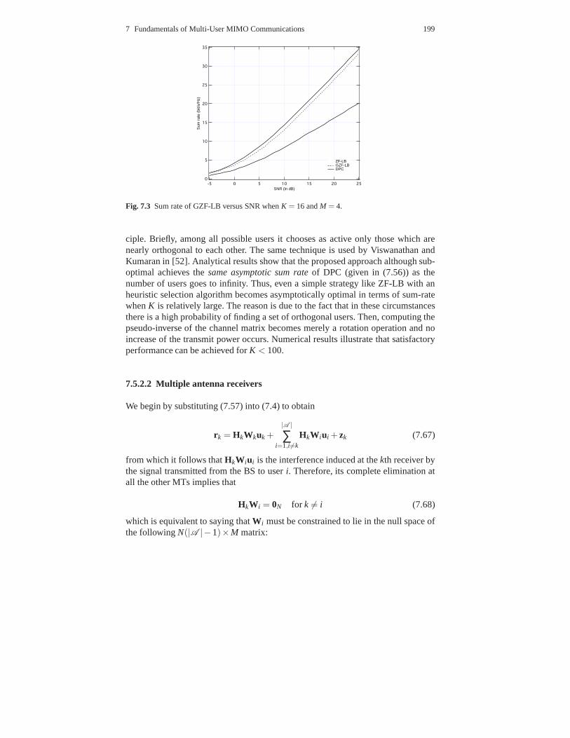
7 Fundamentals of Multi-User MIMO Communications 199
35
30
25
20
15
10
5
0
Sum
rat
e (b
it/s/
Hz)
2520151050-5
SNR (in dB)
ZF-LB GZF-LB DPC
Fig. 7.3 Sum rate of GZF-LB versus SNR whenK = 16 andM = 4.
ciple. Briefly, among all possible users it chooses as activeonly those which arenearly orthogonal to each other. The same technique is used by Viswanathan andKumaran in [52]. Analytical results show that the proposed approach although sub-optimal achieves thesame asymptotic sum rateof DPC (given in (7.56)) as thenumber of users goes to infinity. Thus, even a simple strategylike ZF-LB with anheuristic selection algorithm becomes asymptotically optimal in terms of sum-ratewhenK is relatively large. The reason is due to the fact that in these circumstancesthere is a high probability of finding a set of orthogonal users. Then, computing thepseudo-inverse of the channel matrix becomes merely a rotation operation and noincrease of the transmit power occurs. Numerical results illustrate that satisfactoryperformance can be achieved forK < 100.
7.5.2.2 Multiple antenna receivers
We begin by substituting (7.57) into (7.4) to obtain
r k = HkWkuk +|A |
∑i=1,i 6=k
HkW iui +zk (7.67)
from which it follows thatHkW iui is the interference induced at thekth receiver bythe signal transmitted from the BS to useri. Therefore, its complete elimination atall the other MTs implies that
HkW i = 0N for k 6= i (7.68)
which is equivalent to saying thatW i must be constrained to lie in the null space ofthe followingN(|A |−1)×M matrix:

200 Luca Sanguinetti and H. Vincent Poor
H i = [HT1 , . . . ,HT
i−1,HTi+1, . . . ,H
T|A |]
T . (7.69)
As discussed in [45] and [13], this can be achieved by settingW i = V′
i whereV′
i isobtained from the singular value decomposition (SVD) ofH i . It is worth noting thatthe same goal can be obtained with lower complexity using a QR-based decompo-sition approach as shown by Chenet al. in [11]. In the sequel, however, we resort tothe SVD which produces
H i =[
Ui U′
i
]
[
Di 00 0
]
[
V i V′
i
]H(7.70)
whereV′
i is composed by the right singular vectors associated to theM−N(|A |−1)
null singular values ofH i . ReplacingW i with V′
i in (7.67) produces
r k = H′
kuk +zk for k = 1,2, ..., |A | (7.71)
where we have definedH′
k = HkV′
k. From the above equation, it is seen that themulti-user interference has been completely at each MT. It is worth observing that asufficient condition to guarantee the existence of such a solution is that the numberM −N(|A | − 1) of non-zero singular values is larger thanN. This impliesM ≥N |A |.
Letting H′= diag{H
′
1,H′
2, . . . ,H′
|A |}, the maximum sum rate under the BD con-straint can be computed as
RBD−ZF = max{S≥0, tr(S)≤ p}
log∣
∣
∣IN + H
′SH
′H∣
∣
∣(7.72)
from which it easily follows that the optimalS can be computed by means of thewater-filling algorithm over the effective block diagonal channel matrixH
′[46].
Similarly to ZF-LB, RmaxBD−ZF is obtained maximizing over all possible setsA so
thatN |A | ≤ M, i.e.,
RmaxBD−ZF = max
A ⊂{1,2,...,K},N|A |≤MRBD−ZF. (7.73)
As observed for ZF-LB, a brute force search of the optimal user set is prohibitive asit has combinatorial complexity. To reduce this complexity, two suboptimal greedyalgorithms have been recently proposed by Shenet al. in [44]. The first selects theuser with the highest sum rate and then chooses from the remaining ones that pro-vide the largest sum rate increase with the other already selected. The algorithmterminates when|A | = M/N users are taken or when the sum rate drops if moreusers are chosen. Although reasonable, such a solution is still too computationallyintensive as it requires the computation of an SVD at each iteration in order to evalu-ate the sum rate of each possible user. The second approach has lower complexity asit is based on the maximization of the Frobenius norm of the effective channel. Therationale behind this scheme is that the sum rate is closely related to the eigenval-ues of the effective channel whose sum is exactly the Frobenius norm. Numerical

7 Fundamentals of Multi-User MIMO Communications 201
results show that both algorithms achieve about 95% of the sum rate of the solu-tion obtained through complete search even though their complexities increase onlylinearly with K instead of exponentially as the optimal one does. Both algorithms,however, incur a non-negligible loss with respect to DPC.
7.6 Limited feedback systems
The main drawbacks of the aforementioned transmission schemes is that they re-quire perfect CSI at the transmitter. In Section 3, we have discussed how this infor-mation can be achieved in open- and closed-loop systems and we have also pointedout the large number of technical challenges arising in suchsystems. All this has re-cently stimulated substantial interest toward the development of different solutionsthat may attain the potential gains of MIMO GBCs using a relatively small amountof information. They are commonly referred to aslimited or finite-rate feedbacksystems [33]. Albeit this topic is still much open, some interesting solutions haverecently been proposed (see for example the tutorial paper of Love et al. [34] andthe corresponding special issue [23] for a fairly complete list of references).
7.6.1 Channel quantization
The simplest approach to limit the feedback information relies on the efficient quan-tization of the channel estimates before transmission. In systems with a limited num-ber of users (in the order ofM) a well-studied approach is based on feeding backonly the directions of the estimated channel vectors while no information about thechannel magnitudes is conveyed to the transmitter. The rationale behind this ap-proach is that channel magnitudes play a key role whenK is much larger thanM.In fact, only in this case they can potentially be used by a user selection algorithmto exploit the multi-user diversity of the system. To obtainfurther insights into thisstrategy, in the following we review its basic ideas in the single receive antennascenario. Thekth generic user (k = 1,2, . . . ,K) computes an estimatehk of hk andquantizes the corresponding directionhk/
∥
∥hk
∥
∥ to the channel quantization vectorhk. The latter is chosen from a codebookJk different from one user to the other andcomposed ofJ = 2B unit norm vectors, i.e.,Jk = {fk,1, fk,2, . . . , fk,J} with
∥
∥fk,i
∥
∥= 1.As in the single user case, thekth MT computeshk as follows:
hk = fk,n (7.74)
where the indexn is chosen according to the minimum distance criterion
n = arg maxi=1,2,...,J
∣
∣hHk fk,i
∣
∣ . (7.75)

202 Luca Sanguinetti and H. Vincent Poor
Since the codebook can be designed off-line and known to the transmitter and re-ceiver, each user needs to send back to the transmitter only the selected indexn,meaning that the total number of feedback bits is given byB. In single-user applica-tions with multiple transmit and receive antennas, it has been shown that selectingBequal to the number of transmit antennas is enough to achievealmost the same per-formance as a system operating with perfect channel knowledge at the transmitter.A different result has been found by Jindalet al. in [30] for a multi-user setting inwhich K is equal toM and theJ quantization vectors are chosen from the isotropicdistribution on theM−dimensional unit sphere. In particular, the author shows thatin such a case the sum rate of a ZF-LB scales optimally only when the number offeedback bits per user increaseslinearly with both the number of transmit antennasand the SNR (in dB), i.e.,
B≈ ρ (M−1) logSNR (7.76)
whereρ ≥ 1 is a design parameter. The above result is motivated by the fact that ina multi-user environment (unlike the single-user case) anymismatch in the CSI atthe transmitter leads not only to a reduction of the receivedSNR at the MTs but alsoto an increase of the multiple access interference since theZF condition is no longervalid. In the high SNR regime, this effect is much more harmful than a reduction ofthe desired signal power (as it happens in the single-user case) and, thus, a largernumber of bits is required.
A possible way to alleviate this problem is discussed in [62]where each usersends back to the transmitter not only the directions of the estimated channel vec-tors but also an unquantized channel quality indicator based on the SINR. This isthen used at the BS to perform user selection so as to exploit the multi-user diver-sity, thereby leading to a substantial improvement of the system performance. Inparticular, it turns out that the number of feedback bits required to achieve the sameasymptotic performance of a system with perfect CSI can be computed as follows:
B≈ ρ (M−1) logSNR+ logK (7.77)
from which it follows that for a given value of SNR it largely decreases as thenumber of usersK increases.
7.6.2 Random beamforming
Alternative solutions are based on therandom beamforming(RBF) technique, whichwas originally proposed in [55] for the single-user scenario and later extended to themulti-user case in [42]. The basic idea behind this solutionis to process the user datastreams withM orthonormal beamforming vectors, which are randomly generatedat each transmission time according to an isotropic distribution. At the remote ends,each receive antenna acts as aneffectiveuser (no cooperation is assumed) whichmeasures the received SINRs corresponding to all theM transmit beamforming vec-

7 Fundamentals of Multi-User MIMO Communications 203
tors (this can be easily achieved by means of a properly designed training phase).Once all these estimates are obtained, each effective user selects and conveys backto the transmitter its maximum SINR along with the corresponding beamformingindex. This information is then used at the BS to decide according to the maximumsum rate criterion which set of effective users must be served or not. Surprisingly,when the number of users is relatively large, these bandwidth-efficient scheme (onlyone real-valued parameter and an integer number per effective user) is asymptoti-cally optimal as the sum rate of the system scales likeM log logK. This is madepossible by multi-user diversity which enables even a random beamforming vec-tor to be closely matched to certain users. In [70], a furtherreduction of feedbackinformation is achieved using random beamforming in conjunction with a receiveantenna selection algorithm and an efficient SINR quantization technique. Numeri-cal results show that both the above solutions work properlywhenK is on the orderof hundreds. In practical applications, however,K is likely to be much smaller and alarge degradation of the system performance may occur. Possible solutions to alle-viate this problem are discussed in [25] and [58]. Both schemes rely on the idea ofusing the feedback SINRs not only to select the active users but also to dynamicallyallocate the transmit power among the random beamforming directions. In this way,less or even no power can be assigned to those beams which are not aligned to anyuser channel.
7.6.3 Transceiver optimization
In addition to the aforementioned techniques, considerable recent interest has beendevoted to alternative solutions that are essentially based on the joint optimization oftransmitter and receivers [36] through the use of limited feedback and feedforwardlinks (see for example [9] and [10]). Although powerful, these approaches ofteneither lead to a complicated iterative procedure or requirean excessive overhead ofexchanged information.
7.7 Conclusions
In this chapter, we have reviewed a number of key concepts forunderstanding theuplink and downlink issues of a general multi-user mobile communication systemoperating with multiple antennas at both the BS and MTs. The first part of the chap-ter has focused on the computation of the capacity as a means for characterizingsuch systems. To this end, we have considered various operating conditions that sub-stantially account for different degrees of CSI available at the transmitter(s) and/orreceiver(s). In particular, it has been shown that in the uplink the capacity is, in mostof the cases under investigation, a well-established result whose computation can beformulated as a convex optimization problem. On the other hand, it has been pointed

204 Luca Sanguinetti and H. Vincent Poor
out that in the downlink the problem is a more challenging task whose solution hasrecently been computed using the duality principle and the DPC technique, but onlyfor the case of perfect channel knowledge at the transmitter. Unfortunately, much isstill unknown in the other cases of interest. On the basis of the information-theoreticresults provided, we have also made evident the fact that in the downlink CSI at thetransmitter plays a key role in exploiting the promising gains of multiple antennas.For this purpose, we have briefly described how this information can be acquired byresorting to two different operating techniques, namely, open-loop and closed-loop.
The second part of the chapter has been devoted to analyzing practical issuesin the design of these systems. Most of this analysis has focused on the downlink,as the uplink has been shown to be reminiscent of other well-investigated commu-nication systems. Among the large number of existing solutions, we have focusedour attention on two simple linear transmit beamforming techniques based on thezero-forcing criterion. Both require perfect CSI at the transmitter and exhibit goodtradeoffs between performance and complexity, especiallywhen the number of usersis large.
Finally, in the last part of the chapter, we have examined briefly the issue oflimited feedback, which has been the topic of considerable recent research activity.In particular, we have described some techniques that may provide benefits nearlyidentical to systems with perfect CSI at the transmitter, and we have made somecomments on promising directions for future research in this area.
References
1. Ahslwede, R. (1971) Multi-way communication channels. In Proceedings of the IEEE Inter-national Symposium on Information Theory (Tsahkadsor, Armenian S.S.R.),Budapest, Hun-gary: Akademiai Kiado, June, pp. 23 – 52.
2. Amraoui A., Kramer, G. and Shamai (Shitz), S. (2003) Coding for the MIMO broadcast chan-nel. In Proceedings of the IEEE International Symposium on Information Theory,PacificoYokohama, Kanagawa, Japan, June 29 – July 4, p. 296.
3. Bergman, P. (1973) Random coding theorem for broadcast channels with degraded compo-nents.IEEE Transactions on Information Theory,vol. 19 (3), pp. 197 – 207.
4. Biglieri, E., Proakis, J., and Shamai (Shitz), S. (1998) Fading channels: Information-theoreticand communications aspects.IEEE Transactions on Information Theory,vol. 44 (6) pp. 2619– 2692.
5. Biglieri, E., Calderbank, R., Constantinides, A., Goldsmith, A., Paulraj, A., and Poor, H. V.(2007)MIMO Wireless Communications,Cambridge, UK: Cambridge University Press.
6. Bolcskei, H., Gesbert, D., Papadias, C. B., and Van Der Veen, A.-J. (2006)Space-Time Wire-less Systems: From Array Processing to MIMO Communications, Cambridge, UK: Cam-bridge University Press.
7. Boyd, S., and Vanderbenghe, L. (2003)Convex Optimization.Cambridge, UK: CambridgeUniversity Press.
8. Caire, G., and Shamai (Shitz), S. (2003) On the achievablethroughput of a multiantennaGaussian broadcast channel.IEEE Transactions on Information Theory,vol. 49 (7) pp. 1691– 1706.
9. Chae, C.-B., Mazzarese, D., and Heath, R. W., Jr. (2006) Coordinated beamforming for mul-tiuser MIMO systems with limited feedforward. InProceedings of the Asilomar Conference

References 205
on Signals, Systems and Computers,Pacific Grove, CA, USA, Oct. 30 – Nov. 1, pp. 1511 –1515.
10. Chae, C.-B., Mazzarese, D., Jindal N., and Heath, R. W., Jr. (2008) Coordinated beamformingwith limited feedback in the MIMO broadcast channel.IEEE Journal on Selected Areas inCommunications. Special issue on Limited Feedback.To appear in October 2008.
11. Chen, R., Heath, R. W., Jr., and Andrews, J. G. (2007) Transmit selection diversity for unitaryprecoded multiuser spatial multiplexing systems with linear receivers.IEEE Transactions onInformation Theory,vol. 55 (3) pp. 1159 – 1171.
12. Cheng, R., and Verdu, S. (1993) Gaussian multiaccess channels with ISI: Capacity region andmultiuser water-filling.IEEE Transactions on Information Theory,vol. 21 (5) pp. 684 – 702.
13. Choi, L., and Murch, R. D. (2004) A transmit preprocessing technique for multiuser MIMOsystems using a decomposition approach.IEEE Transactions on Wireless Communications,vol. 3 (1) pp. 20 – 24.
14. Cover, T., (1972) Broadcast channels.IEEE Transactions on Information Theory,vol. 18 (1)pp. 2 – 14.
15. Cover, T. M., and Thomas, J. A. (1991)Elements of Information Theory.New York: Wiley-Interscience.
16. Costa, M. (1983) Writing on dirty paper.IEEE Transactions on Information Theory,vol. 29(3) pp. 439 – 441.
17. Dias, A. R., Bateman, D., and Gosse, K. (2004) Impact of RFfront-end impairments and mo-bility on channel reciprocity for closed-loop multiple antenna techniques. InProceedings ofthe IEEE International Symposium on Personal, Indoor and Mobile Radio Communications,Barcelona, Spain, Sept. 05 – 08, vol. 2, pp. 1434 – 1438.
18. Dimic, G., and Sidiropoulos, N. D. (2005) On downlink beamforming with greedy user se-lection: Performance analysis and a simple new algorithmIEEE Transactions on Signal Pro-cessing,vol. 53 (10) pp. 3857 – 3868.
19. Erez, U., and ten Brink, S. (2005) A close to capacity dirty paper coding scheme.IEEETransactions on Information Theory,vol. 51 (10) pp. 3417 – 3432.
20. Foschini, G. J. (1996) Layered space-time architecturefor wireless communications in fadingenvironments when using multi-element antennas.Bell Labs Technical Journal,vol. 1 (2) pp.41 – 59.
21. Foschini, G. J. and Gans, M. J. (1998) On limits of wireless communications in a fadingenvironment when using multiple antennas.Wireless Personal Communications,vol. 6 (2)pp. 331 – 320.
22. Goldsmith, A., Jafar, S. A., Jindal, N., and Vishwanath,S. (2003) Capacity limits of MIMOchannels.IEEE Journal on Selected Areas in Communications,vol. 21 (5) pp. 684 – 702.
23. IEEE Journal on Selected Areas of Communications. Special issue on Limited Feedback. Toappear in October 2008.
24. Knopp, R., and Humblet, P. A. (1995) Information capacity and power control in single-cell multi-user communications. InProceedings of the IEEE International Conference onCommunications,Seattle, WA, June, vol. 1, pp. 331 – 335.
25. Kountouris, M. and Gesbert, D. (2005) Robust multi-useropportunistic beamforming forsparse networks. InProceedings of the IEEE Workshop on Signal Processing Advances inWireless Communications,New York, NY, June 5 – 8, pp. 975 – 979.
26. Jafar, S., and Goldsmith, A. (2004) Isotropic fading vector broadcast channels: The scalarupper bound and loss in degrees of freedom.IEEE Transactions on Information Theory,vol.51 (3) pp. 848 – 857.
27. Jindal, N., Vishwanath, S., and Goldsmith, A. (2004) On the duality of Guassian multiple-access and broadcast channels.IEEE Transactions on Information Theory,vol. 50 (5) pp. 768– 783.
28. Jindal, N., Rhee, W., Vishwanath, S., Jafar, S. A., and Goldsmith, A. (2005) Sum poweriterative water-filling for multi-antenna Gaussian broadcast channels.IEEE Transactions onInformation Theory,vol. 51 (4) pp. 1570 – 1580.
29. Jindal, N., and Goldsmith, A. (2005) Dirty-paper codingversus TDMA for MIMO broadcastchannels.IEEE Transactions on Information Theory,vol. 51 (5) pp. 1783 – 1794.

206 Luca Sanguinetti and H. Vincent Poor
30. Jindal, N. (2006) MIMO broadcast channels with finite rate feedback.IEEE Transactions onInformation Theory,vol. 52 (11) pp. 5045 – 5059.
31. Joham, M., Kusume, K., Gzara, M. H., and Utschick, W. (2004) Transmit Wiener filter for thedownlink of TDD DS-CDMA systems. InProc. of the IEEE Symposium on Spread-SpectrumTechnologies and Applications,Lisbon, Portugal, Sept. 15 – 18, pp. 9 – 13.
32. Lee, J., and Jindal, N. (2007) High SNR Analysis for MIMO broadcast channels: Dirty papercoding versus linear precoding.IEEE Transactions on Information Theory,vol. 53 (12) pp.4787 – 4792.
33. Love, D. J., Heath, R. W., Jr., Santipach, W. and Honig, M.L. (2003) What is the value oflimited feedback for MIMO channels?IEEE Communications Magazine,vol. 42 (10) pp. 54– 59.
34. Love, D. J. and Heath, R. W., Jr., Lau, V. K. N., Gesbert, D., Rao, B. D., and Andrews, M.(2008) An overview of limited feedback in wireless communication systems.IEEE Journal onSelected Areas in Communications. Special issue on LimitedFeedback.To appear in October2008.
35. Marton, K. (1979) A coding theorem for the discrete memoryless broadcast channel.IEEETransactions on Information Theory,vol. 23 (3) pp. 306 – 311.
36. Pan, Z., Wong, K.-K., and Ng, T.-S. (2004) Generalized multiuser orthogonal space-divisionmultiplexing.IEEE Transactions on Wireless Communications,vol. 3 (6) pp. 1969 – 1973.
37. Peel, C. B., Hochwald, B. M., and Swindlehurst, A. L. (2005) A vector perturbation tech-nique for near capacity multiantenna mutliuser communication - Part I: Channel inversionand regularization.IEEE Transactions on Communications,vol. 53 (1) pp. 195 – 202.
38. Poor, H. V. (2004) Iterative multi-user detection.IEEE Signal Processing Magazine,vol. 21(1) pp. 81 – 88.
39. Rhee, W., and Cioffi, J. M. (2003) On the capacity of multi-user wireless channels with mul-tiple antennas.IEEE Transactions on Information Theory,vol. 49 (10) pp. 2580 – 2595.
40. Rimoldi, R., and Urbanke, R. (1996) A rate-splitting approach to the Gaussian multiple-accesschannel.IEEE Transactions on Information Theory,vol. 46 (2) pp. 364 – 375.
41. Sato, H. (1978) An outer bound on the capacity region of broadcast channels.IEEE Transac-tions on Information Theory,vol. 24 (3) pp. 374 – 377.
42. Sharif, M., and Hassibi, B. H. (2005) On the capacity of MIMO broadcast with partial sideinformation.IEEE Transactions on Information Theory,vol. 51 (2) pp. 506 – 522.
43. Sharif, M., and Hassibi, B. (2007) A comparison of time-sharing, DPC, and beamforming forMIMO broadcast channels with many users.IEEE Transactions on Communications,vol. 55(1) pp. 11 – 15.
44. Shen, Z., Chen, R., Andrews, J. G. and Heath, R. W., Jr. (2006) Low complexity user selectionalgorithm for multiuser MIMO systems with block diagonalization. IEEE Transactions onSignal Processing,vol. 54 (9) pp. 3658 – 3663.
45. Spencer, Q. H., Swindlehurst, A. L. and Haardt, M. (2004)Zero-forcing methods for thedownlink spatial multiplexing in multi-user MIMO channels. IEEE Transactions on SignalProcessing,vol.52 (2) pp. 461 – 471.
46. Telatar, E. (1999) Capacity of multi-antenna Gaussian channels.European Transactions onTelecommunications,vol. 10 (6) pp. 585 – 595.
47. Tong, L., Sadler, B. M. and Dong, M. (2004) Pilot-assisted wireless transmissions.IEEESignal Processing Magazine,vol. 21 (6) pp. 12 – 25.
48. Tse, D., and Hanly, S. V. (1998) Multiaccess fading channels - Part I : Polymatroid structure,optimal resource allocation and throughput capacities.IEEE Transactions on InformationTheory,vol. 44 (7) pp. 2796 – 2815.
49. Tse, D., and Viswanath, P. (2005)Fundamentals of Wireless Communications.Cambridge,UK: Cambridge University Press.
50. Vandenberghe, L., Boyd, S., and Wu, S. P. (1998) Determinant maximization with linearmatrix inequality constraints.SIAM Journal Matrix Analytical Applications,vol. 19 (2) pp.499 – 533.
51. Verdu, S. (1998)Multiuser Detection.Cambridge, UK: Cambridge University Press.

References 207
52. Viswanathan, H., and Kumaran, K. (2001) Rate schedulingin multiple antenna downlinkwireless systems. InProceedings of the Allerton Conference on Communications,Controland Computing,Monticello, IL, USA, Sept. 29 – Oct. 1, vol. 39, pp. 747 – 756.
53. Viswanathan, H., Venkatesan, S., and Huang, H. (2003) Downlink capacity evaluation ofcellular networks with known-interference cancellation.IEEE Journal on Selected Areas ofCommunications,vol. 21 (6) pp. 802 – 811.
54. Viswanath, P., Tse, D., and Anantharam, V. (2001) Asymptotically optimal water-filling invector multiple-access channels.IEEE Transactions on Information Theory,vol. 47 (1) pp.241 – 267.
55. Viswanath, P., Tse, D., and Laroia, R. (2002) Opportunistic beamforming using dumb anten-nas.IEEE Transactions on Information Theory,vol. 48 (6) pp. 1277 – 1294.
56. Viswanath, P., and Tse, D. (2003) Sum capacity of the vector Gaussian channel and uplink-downlink duality.IEEE Transactions on Information Theory,vol. 49 (8) pp. 1912 – 1921.
57. Vishwanath, S., Jindal, N., and Goldsmith, A. (2003) Duality, achievable rates and sum ratecapacity of Gaussian MIMO broadcast channels.IEEE Transactions on Information Theory,vol. 49 (10) pp. 2658 – 2668.
58. Wagner, J. , Liang, Y.-C., and Zhang R. (2007) On the balance of multiuser diversity andspatial multiplexing gain in random beamforming.IEEE Transactions on Wireless Communi-cations.vol. 7 (7) pp. 2512 – 2525.
59. Wang, X., and Poor, H. V. (2004)Wireless Communication Systems: Advanced Techniquesfor Signal Reception.Upper Saddle River, NJ: Prentice-Hall.
60. Weingarten, H., Steinberg, Y., and Shamai (Shitz), S. (2006) The capacity region of the Gaus-sian multiple-input multiple-output broadcast channel.IEEE Transactions on InformationTheory,vol. 50 (9) pp. 3936 – 3964.
61. Yoo, T., and Goldsmith, A. (2006) On the optimality of multiantenna broadcast schedulingusing zero-forcing beamforming.IEEE Journal on Selected Areas in Communications,vol.25 (7) pp. 1478 – 1491.
62. Yoo, T., Jindal, N., and Goldsmith, A. (2007) Multi-antenna downlink channels with limitedfeedback and user selection.IEEE Journal on Selected Areas in Communications,vol. 25 (7)pp. 1478 – 1491.
63. Yu, W., Rhee, W., and Cioffi, J. M. (2001) Optimal power control in multiple-access fad-ing channels with multiple antennas. InProceedings of IEEE International Conference onCommunications,Helsinki, Finland, June 11 – 14, pp. 575 – 579.
64. Yu, W., Sutivong, A., Julian, D., Cover, T. M., and Chiang, M. (2001) Writing on coloredpaper. InProceedings of IEEE International Symposium on Information Theory,Washington,DC, USA, June 24 – 29, pp. 302 – 311.
65. Yu, W., Rhee, W., Boyd, S., and Cioffi, J. M. (2004) Iterative water-filling for Gaussian vectormultiple-acess channels.IEEE Transactions on Information Theory,vol. 50 (1) pp. 145 – 152.
66. Yu, W., and Cioffi, J. M. (2004) Sum capacity of the vector Gaussian channels.IEEE Trans-actions on Information Theory,vol. 50 (9) pp. 1875 – 1892.
67. Yu, W., Varodayan, D. P., and Cioffi, J. M. (2005) Trellis and convolutional precoding fortransmitter-based interference pre-cancellation.IEEE Transactions on Information Theory,vol. 53 (7) pp. 1220 – 1230.
68. Yu, W. (2006) Sum-capacity computation for the Gaussianvector broadcast channel via dualdecomposition.IEEE Transactions on Information Theory,vol. 52 (2) pp. 754 – 759.
69. Yu, W., and Rhee, W. (2006) Degrees of freedom in wirelessmultiuser spatial multiplexsystems with multiple antennas.IEEE Transactions on Communications,vol. 54 (10) pp.1747 – 1753.
70. Zhang, W., and Letaief, K. B. (2007) MIMO broadcast scheduling with limited feedback.IEEE Journal on Selected Areas in Communications. Special issue on MIMO Transceiversfor Realistic Communication Networks: Challenges and Opportunities,vol. 25 (7) pp. 1457– 1467.


