ADB Working Paper Series on Regional Economic Integration · PDF fileADB Working Paper Series on Regional Economic Integration ... Macroeconomic Forecasting, Global vector ... to develop

ASEAN-5 Macroeconomic Forecasting Using a GVAR Model

Fei Han and Thiam Hee NgNo. 76 | March 2011

ADB Working Paper Series onRegional Economic Integration

ADB Working Paper Series on Regional Economic Integration

ASEAN-5* Macroeconomic Forecasting Using a GVAR Model

Fei Han+ and Thiam Hee Ng++

No. 76 March 2011

*ASEAN-5 in this paper refers to the original five ASEAN members: Indonesia, Malaysia, Philippines, Singapore, and Thailand. The authors would like to thank Lei Lei Song and Renato E. Reside for their helpful suggestions and valuable comments. The authors also wish to give special thanks to OREI ADB consultants Julie Ann Basconcillo for her help in computing the trade weights, and Marthe Hinojales for helping apply StataCorp LP’s STATA software. Any errors are our own. +Fei Han is an intern, Office of Regional Economic

Integration, Asian Development Bank, and a PhD Candidate, University of California, Berkeley. email: [email protected] ++

Thiam Hee Ng is Economist, Office of Regional Economic Integration, Asian Development Bank, 6 ADB Avenue, Mandaluyong City, 1550 Metro Manila, Philippines. Tel: +63 2 632 4522, Fax: +63 2 636 2342, email: [email protected]

The ADB Working Paper Series on Regional Economic Integration focuses on topics relating to regional cooperation and integration in the areas of infrastructure and software, trade and investment, money and finance, and regional public goods. The Series is a quick-disseminating, informal publication that seeks to provide information, generate discussion, and elicit comments. Working papers published under this Series may subsequently be published elsewhere. Disclaimer: The views expressed in this paper are those of the authors and do not necessarily reflect the views and policies of the Asian Development Bank (ADB) or its Board of Governors or the governments they represent. ADB does not guarantee the accuracy of the data included in this publication and accepts no responsibility for any consequence of their use. By making any designation of or reference to a particular territory or geographic area, or by using the term “country” in this document, ADB does not intend to make any judgments as to the legal or other status of any territory or area. Unless otherwise noted, $ refers to US dollars. © 2011 by Asian Development Bank March 2011 Publication Stock No. WPS113351

Contents Abstract v

1. Introduction 1

2. The GVAR Model 2

2.1. Country-Specific VARX* Models 2 2.2. Estimation Strategy 5 2.3. Solution of the GVAR Model 6

3. Data 8

4. Tests 8

4.1. Unit Root Tests 8 4.2. Testing Weak Exogeneity 8 4.3. Other Features of the Country-Specific Models 9 4.4. Contemporaneous Effects of Foreign Variables on

Domestic Counterparts 9

5. Forecast and Evaluation 10

5.1. Forecast Results 10 5.2. Benchmark Models 10 5.3. Forecast Evaluation 11

6. Generalized Impulse Response Functions 12

7. Conclusion 13

Appendix—Data Description 30

A1: Real GDP 30 A2: Consumer Price Index (CPI) 30 A3: Short-Term Interest Rates 30 A4: Exchange Rates 31 A5: Equity Price Indices 31 A6: Fuel and Non-fuel Commodity Price Index 31

References 32

ADB Working Paper Series on Regional Economic Integration 33 Tables

1. Trade Weights Based on Direction of Trade Statistics 14

2. Co-Integration Rank Statistics for the US Model (3 exogenous variables) 14

3. Co-Integration Rank Statistics for Non-US Countries/ East Asia (5 exogenous variables) 15

4. VARX* Order and Number of Co-Integration Relationships in the Country-Specific Models 15

Tables

5. ADF-GLS Unit Root Test Statistics (based on MAIC order selection) 16

6. F-statistics for Testing the Weak Exogeneity of the Country-Specific Foreign Variables and Commodity Prices 17

7. F-statistics for Tests of Residual Serial Correlation for Country-Specific VARX* Models 17

8. Contemporaneous Effects of Foreign Variables on their Domestic Counterparts 18

9. Panel DM Statistics for GVAR Forecasts Relative to the Benchmark Model, 2009Q1–2009Q4 18

Figures

1. One Quarter Ahead Forecasts for Real GDP Growth 19

2. One Quarter Ahead Forecasts for Inflation 20

3. One Quarter Ahead Forecasts for Short-Term Interest Rate 21

4. One Quarter Ahead Forecasts for Real Exchange Rate 22

5. One Quarter Ahead Forecasts for Real Equity Prices 23

6. Generalized Impulse Responses of a Negative Unit (1 s.e.) Shock to US Real Equity Prices 24

7. Generalized Impulse Responses of a Negative Unit (1 s.e.) Shock to US Real Equity Prices (cont.) 25

8. Generalized Impulse Responses of a Positive Unit (1 s.e.) Shock to World Commodity Prices in the US Model 26

9. Generalized Impulse Responses of a Positive Unit (1 s.e.) Shock to World Commodity Prices in the US Model (cont.) 27

10. Generalized Impulse Responses of a Positive Unit (1 s.e.) to US Short-Term Interest Rates 28

11. Generalized Impulse Responses of a Positive Unit (1 s.e.) Shock to US Short-Term Interest Rates (cont.) 29

Abstract This paper examines and evaluates macroeconomic forecasts for the original ASEAN-5 members in the context of a global vector autoregressive (GVAR) model covering 20 countries, grouped into nine countries/regions. After estimating the GVAR model, we generate 12 one-quarter-ahead forecasts for the next quarter including real GDP, inflation, short-term interest rates, real exchange rates, and real equity prices over the period 2009Q1–2011Q4,** with four out-of-sample forecasts over the period 2009Q1–2009Q4. Forecast evaluation results based on the panel Diebold-Mariano (DM) tests show the GVAR forecasts tend to outperform forecasts based on the benchmark country-specific models, especially for short-term interest rates and real equity prices, emphasizing the interdependencies in the global financial market. Keywords: Macroeconomic Forecasting, Global vector autoregressive model (GVAR), Southeast Asia JEL Classification: E37, F47

** Throughout this paper, references such as “2009Q1” refer to the year followed by the specific quarter.

| 1

1. Introduction There are various time series models for macroeconomic forecasting, which can be generally classified into two different approaches: structural approach and reduced-form approach. Although the structural approach is model-oriented and embeds more economic structures, it usually requires building a complex economic model with multiple parameters. As a result, it is more sensitive parameter estimates and underlying assumptions about the economy relative to the reduced-form approach. It is also computationally more intense and difficult to implement in practice—especially when doing macroeconomic forecasting for more than one country. On the other hand, the reduced-form approach is usually more data-oriented and does not incorporate many economic structures, but it is easier to implement with its smaller computational requirements. Most time series models belong to the reduced-form approach. For univariate forecasting, autoregressive moving variable (ARMA) and autoregressive integrated moving variable (ARIMA) models are frequently used in literature for stationary and nonstationary time series, respectively; autoregressive conditional heteroskedasticity/generalized autoregressive conditional heteroskedasticity (ARCH/GARCH) models are useful to model time series with time-varying conditional variance—demonstrating their power for estimation and forecasting in finance. For multivariate stationary time series, the vector autoregressive (VAR) model, a generalization of the univariate autoregressive model, is able to capture the evolution and interdependencies among multiple time series. Sim (1980) proposed a Cholesky decomposition method to solve the well-known identification problem of the original VAR system. However, this VAR approach has been criticized as being devoid of any economic content. Therefore, many economists and econometricians have been trying to come up with new techniques to incorporate the pros of the structural approach into VAR. Sims (1986) and Bernanke (1986) proposed imposing economic restrictions on the regression innovations—known as the Structural Vector Autoregression (SVAR) model. However, one needs to impose too many economic restrictions—(n2-n)/2 restrictions—in an n-variable VAR in order to achieve identification, which is quite difficult and sometimes impossible when there is more than one country in the sample. Besides these technical issues, another important feature of macroeconomic forecasting we need to consider is the increased globalization and interdependency of the world economy. This has important consequences for conducting monetary and financial policies by central bankers and risk management by commercial bankers. The main motivation for this paper is to forecast the main macroeconomic variables for ASEAN-5. Since these five countries all mid-sized, open economies and are highly affected by other world economic powers such as the United States (US), it is necessary for us to take into account these external impacts. In this paper we employ the global vector autoregressive (GVAR) model originally introduced by Pesaran, Schuermann, and Weiner (2004) and further developed by Dees et al. (2007) and Pesaran et al. (2009) to develop a macroeconomic forecasting model for the ASEAN-5 countries. The advantage of the GVAR model is that it not only incorporates

2 | Working Paper Series on Regional Economic Integration No. 76

economic structures and global interdependencies of the world economy into the VAR model, but also avoids the identification problem in VAR. Furthermore, there are major differences in the cross-country correlations of various real variables. For instance, equity returns are much more closely correlated across countries than real GDP growth and inflation. This suggests that different channels of transmission should be considered. The GVAR approach allows us to model these different types of links directly, using trade-weighted observable macroeconomic aggregates and financial variables. The plan of the paper is as follows: Section 2 presents the GVAR model, its assumptions, and the estimation strategy. Section 3 describes the data used. Section 4 presents tests for two assumptions of GVAR, and contemporaneous effects of foreign variables on their domestic counterparts. Section 5 presents the forecasting results and evaluation. Section 6 derives generalized impulse response functions for the analysis of country-specific shocks. Section 7 offers some concluding remarks. 2. The GVAR Model There are two steps in constructing a GVAR model: the country-specific models and the global VAR. In this section, we provide an overview of the GVAR framework describe the country-specific models and explain how the global VAR is constructed. We can thus ensure that the forecasts obtained for different countries are internally coherent within the GVAR modeling framework. 2.1. Country-Specific VARX* Models The country-specific model is a VARX* model1 for each individual country/region. The endogenous variables in most country-specific models include the following core variables:

( )

( ) ( )( )

( )

( )

( )

, 1

ln

ln ln

ln

ln

0.25ln 1 100

ln

it it it

it it i t

it it it

it it it

Sit it

W Wt t

y GDP CPI

CPI CPI

e E CPI

q EQ CPI

r R

p P

π −

=

= −

=

=

= +

=

1 VARX* is a vector autoregressive (VAR) model with weakly exogenous variables.

ASEAN-5 Macroeconomic Forecasting Using a GVAR Model | 3

where: GDPit = nominal gross domestic product of country i during period t (in local currency), CPIit = consumer price index for country i at time t (with the base year at 100), Eit = exchange rate of country i currency at time t in US dollars, EQit = nominal equity price index,

SitR = nominal short-term interest rate per annum, in percent, W

tP = world commodity price index. The typical maturity of short-term interest rates is 3 months. Full details of data sources are given in the Appendix. The US is indexed as country 0, and the exchange rate of the US—E0t—is taken to be 1. In the country-specific model for each country/region other than the US, the endogenous variables are ( ), , , ,it it it it ity r e qπ ; while for the US model,

the endogenous variables are ( )0 0 0 0, , , , Wt t t t ty r q pπ . Note that the endogeneity of the

world commodity price in the US model reflects the large size of the US economy (it alone accounts for about one-quarter of world output in nominal terms). The real equity price is also included as an endogenous variable to capture the financial market shocks.2 The (weak) exogenous variables in the country-specific VARX* models are trade-weighted foreign core macro-variables (denoted by an “*”). In most country-specific models, foreign variables are constructed as

0 0 0

0 0

, , ,

, ,

N N N

it ij jt it ij jt it ij jtj j j

N N

it ij jt it ij jtj j

y w y w e w e

q w q r w r

π π∗ ∗ ∗

= = =

∗ ∗

= =

= = =

= =

∑ ∑ ∑

∑ ∑

The weights wij for i,j = 0,1,…,N3 are trade weights between country i and country j computed using the simple average of monthly total trade of a country/region during the 2007–2009 period. wii is 0 for any country i. Table 1 shows the trade weights within all countries examined here. We use the exogenous variables in Dees et al (2007). In the country-specific model for each country or regional economy other than the US, the exogenous variables are ( ), , , , W

it it it it ty r q pπ∗ ∗ ∗ ∗ , while for the US model, the exogenous

variables are ( )0 0 0, ,t t ty eπ∗ ∗ ∗ .4 The inclusion of only three foreign variables in the US model reflects the importance of US financial markets within the global financial system. Once the variables to be included in the different country models are specified, we begin the modeling following the assumptions in Dees et al. (2007)—that all the country-specific 2 See Dees et al (2007) for choice of variables. The long-term interest rate is not included in this paper as

an endogenous variable as data for ASEAN-5 are unavailable. 3 N= 8, which is the number of countries/regions minus the US used in this paper. 4 Although foreign inflation does not pass the exogeneity test within our sample period, it remains included

because it passes the test for a longer data period.


variables are I(1), the country-specific exogenous variables are weakly exogenous, and that the parameters of the country-specific models remain stable over time. These two assumptions will be tested in section 4. We then proceed to select the order of the individual country VARX*(pi, qi) models, where pi denotes the lag order of endogenous variables (or domestic variables) and qi denotes the lag order of exogenous variables (or foreign variables). In the empirical analysis that follows, we examine the case where pi is selected according to the Akaike information criterion (AIC). Due to data limitations, the lag order of the foreign variables, qi, is ”1“ for all countries/regions. For the same reason, the maximum pi is not allowed to be greater than two. Based on the AIC values, a VARX*(2, 1) model is fitted to all 9 countries/regions except Japan, Singapore, and Thailand, where the VARX*(1, 1) model is fitted. Therefore, for all countries except those three, the country-specific VARX*(2, 1) models can be written as

0 1 1 , 1 2 , 2 0 1 , 1it i i i i t i i t i it i i t itX h h t X X X X ε∗ ∗− − −= + +Φ +Φ +Ψ +Ψ + (1)

where t is a linear time trend, and; for the US

( ) ( )0 0 0 0 0 0 0 0 0, , , , , , ,Wt t t t t t t t t tX y r q p X y eπ π∗ ∗ ∗ ∗′ ′= = .

For the eurozone, the People’s Republic of China (PRC), Indonesia, Malaysia, and the Philippines, it is

( ) ( ), , , , , , , , , Wit it it it it it it it it it it tX y r e q X y r q pπ π∗ ∗ ∗ ∗ ∗ ′′= = .

The VARX*(1, 1) specification is fitted to Japan, Singapore, and Thailand:

0 1 1 , 1 0 1 , 1it i i i i t i it i i t itX h h t X X X ε∗ ∗− −= + +Φ +Ψ +Ψ + (2)

where: ( ) ( ), , , , , , , , , Wit it it it it it it it it it it tX y r e q X y r q pπ π∗ ∗ ∗ ∗ ∗ ′′= = . It is easy to see that the

VARX*(1, 1) specification in equation (2) can be rewritten as equation (1) with 1 0iΨ = . The error term itε is assumed to be a serially uncorrelated and a weak dependent process cross-sectionally, such that for each t and i, and the set of granular weights wij, we have5

0

0, as .N

Pit ij jt

j

w Nε ε∗

=

= ⎯⎯→ →∞∑

5 See Pesaran et al. (2009) and Pesaran et al. (2004) for a discussion of this assumption and the definition

of granular weights.


2.2. Estimation Strategy There are two main system approaches to estimate the country-specific VARX* models (1) and (2). The first uses Johansen (1988, 1992) and Pesaran, Shin, and Smith’s (2000) fully parametric approach based on a vector autoregressive error correction model. The second utilizes Phillips’ (1991, 1995) semi-parametric procedure based on a triangular formulation of a vector correction model. Although Phillips’ approach is robust to the error distribution and Pesaran et al.’s approach relies on the assumption that errors are normally distributed, Phillips’ nonparametric correction term is more data-demanding. Due to data limitations, we use Pesaran, Shin, and Smith’s (2000) approach in this paper. Let ,i t i t i tZ X X ∗

′⎛ ⎞′′= ⎜ ⎟⎝ ⎠

, a vector of both exogenous and endogenous variables for country

i, and let ik and ik ∗ denote the numbers of domestic and foreign variables in country i respectively. Then the error correction model for both the VARX*(2, 1) specification (1) and the VARX*(1, 1) specification (2) can be written as

0 , 1 0 , 1it i i i i t i it i i t itX c Z X Xα β ε∗ ∗− −′Δ = + +Ψ Δ +Γ Δ + (3)

where 0iΓ = for the VARX*(1, 1) specification, ( , )it itZ t Z∗ ′ ′= , iα is a i ik r× matrix of

rank ri, and iβ is a ( )i i ik k r∗+ × matrix of rank ri. By partitioning iβ as

( , , )i it ix ixβ β β β ∗′ ′ ′ ′= conformable to , 1i tZ ∗

− , the ri error-correction terms defined by the above equation can be written as

, 1 , 1 , 1( 1)i i t it ix i t i tixZ t X Xβ β β β ∗

∗ ∗− − −′ ′ ′ ′= − + + , (4)

which clearly allows for the possibility of co-integration both within Xit and between itX

and itX ∗ , and consequently across Xit and Xjt when i j≠ . Under all assumptions described in section 2.1, the estimation of the vector error correction (VECMX*) model in equation (3) is carried out in three steps. First, iβ is

estimated by the maximum likelihood (ML) estimator ˆiβ proposed in Case IV

(unrestricted intercepts and restricted trends)6 in Pesaran, Shin, and Smith (2000). Second, the rank of iβ , ri, is determined using the maximum eigenvalue and the trace statistics proposed in Pesaran, Shin, and Smith (2000). Third, as shown in Dees et al. (2007), ( )0 0, , ,i i i ic α Ψ Γ ( 0iΓ = in VARX*(1, 1)) can be consistently estimated by

ordinary least squares (OLS) regressions of itXΔ on intercepts, the estimated

error-correction terms ( , 1ˆ

i i tZβ ∗−′ ), itX ∗Δ , and , 1i tX −Δ (no , 1i tX −Δ for VARX*(1, 1)).

6 Here, restricting the time trend is to avoid a quadratic trend in the original model of levels.


The maximum eigenvalues and the trace statistics for all the country-specific models are summarized in Tables 2 and 3. It is known that both of these statistics tend to over-reject in small samples, with the extent of over-rejection being much more serious for the maximum eigenvalue as compared with trace statistics. Using Monte Carlo experiments, it has also been shown that the maximum eigenvalue test is generally less robust to departures from normal errors than trace statistics (see Cheung and Lai 1993). Therefore, we base our inference on trace statistics. Table 4 shows the lag orders and the numbers of co-integration relationships for the country-specific VARX* models. After estimating all the coefficients in equation (3), we can transform them to obtain all the coefficient estimates in the original VARX* models. First, partition i iα β′ as

1 2 3( , , )i i i i ig g gα β ′ = conformable to 1 11, ,t tt X X ∗

− −⎛ ⎞′′−⎜ ⎟⎝ ⎠

. 7 Second, the relationship

between the coefficients in equation (1)/(2) and those in equation (3) can be easily derived as

0 0 1

1 1

1 2

2

1 3 0

i

i i i

i i

i k i i

i i

i i i

h c g

h g

I g

g

⎧ = −⎪⎪ =⎪⎪Φ = + +Γ⎨⎪⎪Φ = −Γ⎪⎪Ψ = −Ψ⎩

where 0iΓ = for the VARX*(1, 1) specification. 2.3. Solution of the GVAR Model Although estimation is done country by country, the GVAR model needs to be solved simultaneously for all endogenous variables in the global economy. Both the VARX*(2, 1) model (1) and the VARX*(1, 1) model (2) can be rewritten as:

0 1 , 1 , 2i it i i i i t i i t itA Z h h t B Z C Z ε− −= + + + + , (5) where:

( )( )

( )

0

1 1

2

, ,

, ,

,0 for VARX*(2, 1), and 0 for VARX*(1, 1),

number of endogenous variables in country .

i

i i

i k i

i i i

i i k k i

i

A I

B

C C

k i

×

= −Ψ

= Φ Ψ

= Φ =

=

7 The notation for estimates ^ is omitted for notational simplicity.


Note that Ai, Bi, and Ci are all ( )i i ik k k∗× + matrixes.

Let ( )0 1, , ,t t t NtX X X X ′′ ′ ′= L be the 1k× global vector of endogenous variables with

0

Nii

k k=

=∑ . The key to solving the model is to note that the link between Xit and the variables in the ith country-specific model Zit can be expressed by the identity

, 0,1, ,it i tZ W X i N= = L (6) where Wi is a ( )i i ik k k∗+ × “link” matrix defined by the trade weights.8 Then, using the identity, equation (5) can be rewritten as 0 1 1 1 2 2i i t i i i i t i i t itAW X h h t B W X B W X ε− −= + + + + where AiWi and Bi1Wi are both ik k× -dimensional matrixes. Stacking these equations now yields

0 1 1 1 2 2t t t tGX h h t H X H X ε− −= + + + + (7)

where:

00 001 0 0 01 0 02 0

10 111 1 1 11 1 12 1

0 1 1 2

0 1 1 2

, , , , , .

t

t

t

N N Nt N N N N N N

h h A W B W B W

h h AW B W B Wh h G H H

h h h A W B W B W

ε

εε

⎛ ⎞ ⎛ ⎞⎛ ⎞ ⎛ ⎞ ⎛ ⎞ ⎛ ⎞⎜ ⎟ ⎜ ⎟⎜ ⎟ ⎜ ⎟ ⎜ ⎟ ⎜ ⎟⎜ ⎟ ⎜ ⎟⎜ ⎟ ⎜ ⎟ ⎜ ⎟ ⎜ ⎟⎜ ⎟ ⎜ ⎟⎜ ⎟ ⎜ ⎟ ⎜ ⎟ ⎜ ⎟= = = = = =⎜ ⎟ ⎜ ⎟⎜ ⎟ ⎜ ⎟ ⎜ ⎟ ⎜ ⎟⎜ ⎟ ⎜ ⎟⎜ ⎟ ⎜ ⎟ ⎜ ⎟ ⎜ ⎟

⎜ ⎟ ⎜ ⎟ ⎜ ⎟ ⎜ ⎟⎜ ⎟ ⎜ ⎟⎝ ⎠ ⎝ ⎠ ⎝ ⎠ ⎝ ⎠⎝ ⎠ ⎝ ⎠

M M M M M M

It is easily seen that G is a k k× -dimensional matrix and, in general, will be of full rank and hence invertible. Then, the GVAR model in all of the variables can be written as

0 1 1 1 2 2t t t tX f f t F X F X u− −= + + + + , (8) where: 1 1 1 1 1

0 0 1 1 1 1 2 2, , , , and t tf G h f G h F G H F G H u G ε− − − − −= = = = = . The global VAR(2) model (8) can then be solved recursively forward for forecasting or generalized impulse response analysis in the usual manner.

8 See the Matlab codes for all the detailed “link” matrixes.


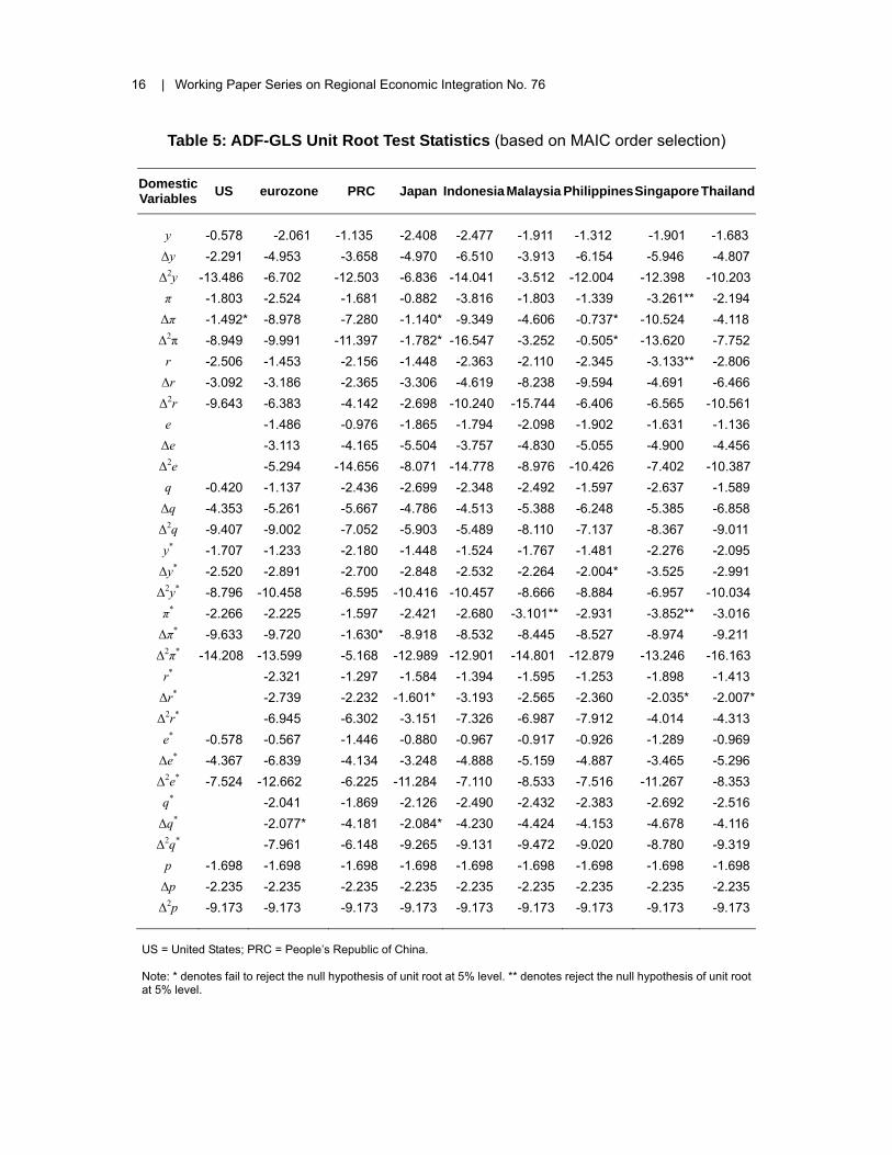
3. Data The quarterly data set used for estimation and forecasting in this paper covers the period 1991Q1–2009Q4, extending the data set in Pesaran et al. (2004) four more years. More specifically, the data used for estimation cover 1991Q1–2008Q4, and the out-of-sample one quarter ahead forecasts are from 2009Q1 to 2009Q4. The main data source is the CEIC database, which includes the International Monetary Fund’s International Financial Statistics (IFS) database and the statistics from national central banks. The nine countries or regional economies considered in this paper are the US, eurozone (Austria, Belgium, France, Germany, Greece, Ireland, Italy, Luxembourg, Netherlands, Portugal, and Spain), the PRC, Japan, and the ASEAN-5. A detailed description of the data which include more countries/regions is provided in the Appendix. 4. Tests 4.1. Unit Root Tests Although the GVAR methodology can be applied to stationary and/or integrated variables, the assumption that the variables included in the country-specific models are integrated of order one (or I(1))—in Pesaran et al. (2004), Dees et al. (2007), and Pesaran et al. (2009)—still plays an important role. The assumption allows us to distinguish short- and long-run relations and interpret those long-run as co-integrating. Therefore, we begin our tests by examining the integration properties of the individual series under consideration. Due to the widely accepted poor power performance of the traditional augmented Dickey-Fuller (ADF) tests, we use the ADF-GLS statistics introduced by Elliot, Rothenberg, and Stock (1996) for all series in Table 5. With only a few exceptions, the I(1) assumption cannot be rejected for most of the endogenous and exogenous variables under consideration.9 4.2. Testing Weak Exogeneity The main assumption underlying the estimation strategy is the weak exogeneity of itX ∗ with respect to the long-run parameters of the VECMX* model defined by (3). Following Dees et al. (2007), we can check the weak exogeneity by testing the joint significance of the estimated error-correction terms defined by (4) for the country-specific foreign variables and world commodity prices. In particular, for each lth element of itX ∗ the following regression is carried out:

, , , , 1 , , 1, , 1 ,1 1

i ir sj

it l il i j l i t ik l i t k i l i t it lj k

X ECM X Xμ γ ϕ υ ς∗ ∗− − −

= =

Δ = + + Δ + Δ +∑ ∑ % (9)

9 Nevertheless, some of the variables used in the country-specific models seem to be I(2), for example, US

inflation, and some even seem to be I(3), for example, Japanese inflation.


where , 1, 1,2, ,ji t iECM j r− = L are the estimated error-correction terms corresponding to

the ri co-integrating relations found for the ith country model, si = pi (the lag order of endogenous variables in the ith country model), and ( , , )W

it it it tX X e p∗ ∗ ∗′ ′Δ = Δ Δ Δ% . Note that

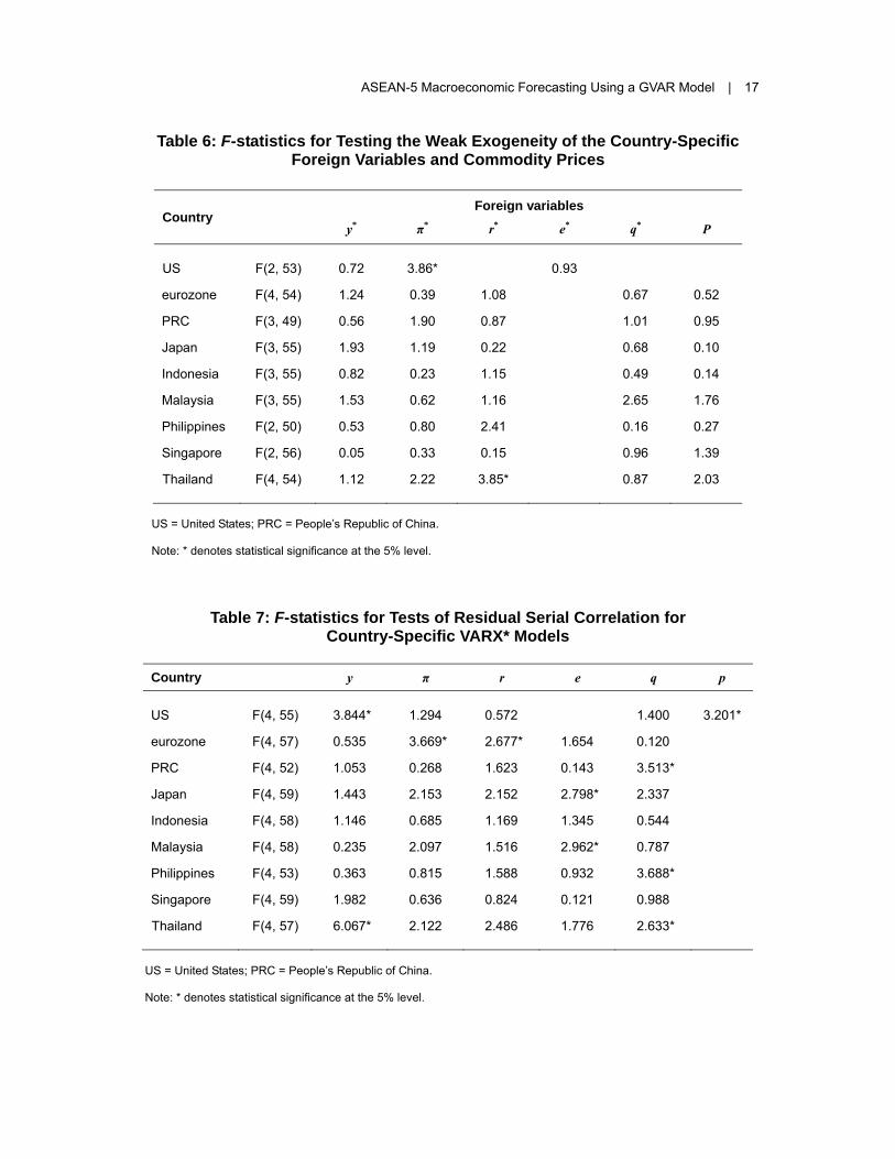
in the case of the US the term ite∗Δ is implicitly included in itX ∗Δ . The test for weak exogeneity is an F-test of the joint hypothesis that , , 0, 1, 2, ,i j l ij rγ = = L in the above regression. The test results are summarized in Table 6. As can be seen from this table, the weak exogeneity assumptions for the countries under consideration are rejected only for inflation in the US model and the short-term interest rate in the Thai model. As expected, foreign real equity prices and foreign short-term interest rates cannot be considered as weakly exogenous and have not been included in the US model, which justifies the importance of US financial markets within the global financial system. 4.3. Other Features of the Country-Specific Models Due to data limitations and the relatively large number of endogenous and exogenous variables involved, we were forced to set the lag order of exogenous variables for all country-specific models at one. It is therefore important to check the adequacy of the country-specific models in dealing with the complex dynamic interrelationships that exist in the world economy. To this end, Table 7 provides F-statistics for Breusch-Godfrey LM tests of serial correlation of order 4 in the residuals of the error-correction regressions for all 45 endogenous variables in the GVAR model. Considering the relative simplicity of the underlying models, it is comforting that 35 of the 45 regressions pass the residual serial correlation test at the 95% level. In particular, if we focus on ASEAN-5, only 4 out of the 20 regressions fail to pass the test at the 95% level. These test results, together with the weak exogeneity of the foreign variables, also allow consistent estimation of the contemporaneous effects of foreign-specific variables on their domestic counterparts (at least for the ones where the residual serial correlation test is not statistically significant). 4.4. Contemporaneous Effects of Foreign Variables on Domestic

Counterparts Table 8 presents the contemporaneous effects of foreign variables on their domestic counterparts together with Newey-West heteroskedasticity and autocorrelation consistent (HAC) covariance matrix estimator. These estimates can be interpreted as impact elasticities between domestic and foreign variables. In Singapore, for example, a 1% change in foreign real GDP in a given quarter leads to an increase of 1.14% in domestic real GDP within the same quarter. Similar foreign elasticities are obtained across the different countries/regions. Most of these elasticities are significant and have a positive sign, which are consistent with the results in Dees et al. (2007), except the foreign short-term interest rate of the


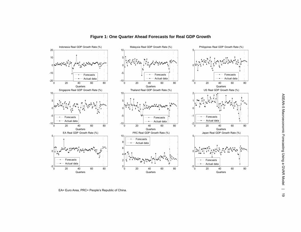
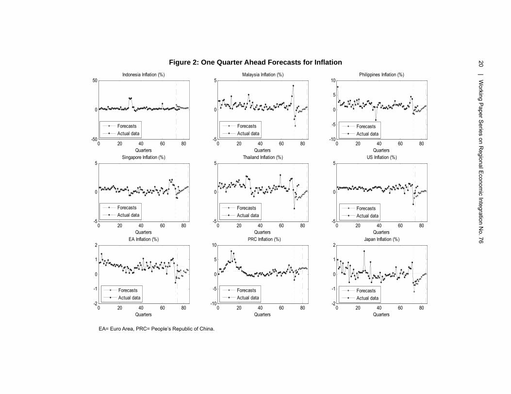
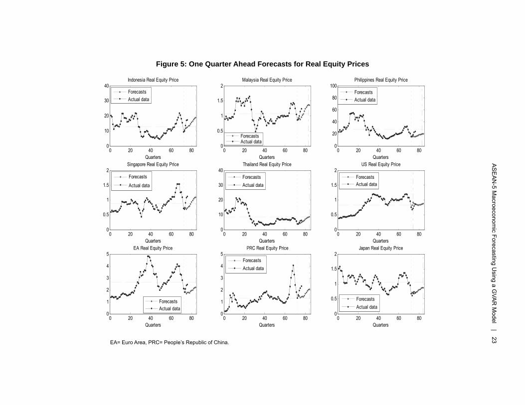
PRC and the foreign inflation of Japan. Focusing on ASEAN-5, foreign real GDP in Malaysia, Singapore, and Thailand, and foreign inflation in Malaysia, the Philippines, and Thailand have significant and positive contemporaneous effects on their domestic counterparts. In addition, the foreign equity prices in all ASEAN-5 countries have significant and positive effects on their domestic counterparts, suggesting contemporaneous financial links are likely to be very strong among ASEAN-5 economies through the equity market channel. Another interesting finding is that neither foreign real GDP nor foreign inflation has a significant effect on their domestic counterparts in the PRC and Indonesia—which may imply the two economies are not as open as the other countries/regions under consideration. 5. Forecast and Evaluation 5.1. Forecast Results We compute the one quarter ahead forecasts for 2009Q1–2011Q4. Figure 1 presents real GDP growth forecasts for all the countries under consideration. We can see that the real GDP growth forecasts for all countries expect Thailand have a clear downward trend in 2011. Figures 2, 3, 4, and 5 present forecasts for inflation, short-term interest rates, real exchange rates, and real equity prices respectively. It is necessary to evaluate how well these forecasts perform compared with other models. We consider two benchmark models used in the forecast evaluation. We apply the panel Diebold and Mariano (DM) test developed by Pesaran et al. (2009)—which allows us to statistically test the GVAR forecasts against our benchmark models for a given variable. Note that we have only four One quarter ahead forecasts (obtained over 2009Q1–2009Q4) for each of the variables and for each country, which is insufficient for statistical testing of forecasts for individual countries. However, by pooling forecast errors for the same variable across different countries, the panel DM test is able to take into account the panel nature of the pooled series. 5.2. Benchmark Models We compare the forecast performance of the GVAR model with that of forecasts from country-specific VAR(2) models, with and without trend. The specifications of the two benchmark models are

1 , 1 2 , 2

1 , 1 2 , 2

Country-specific VAR(2):

Country-specific VAR(2) with trend:

it i t i t it

it i t i t it

X a X X

X a bt X X

γ γ ξ

γ γ ξ

− −

− −

= + + +⎧⎪⎨

= + + + +⎪⎩

where i = 0, 1, 2, …, N. VAR(2) models are chosen for two reasons: (i) they usually perform very well in forecasting; and more importantly, (ii) the only feature they don’t possess compared with the GVAR model is global interdependency. Thus, if the GVAR model outperforms these


VAR(2) models, then the global interrelationships should be considered important in forecasting. The forecast is based on the conditional expectation in the usual manner for VAR models. 5.3. Forecast Evaluation To derive the panel DM test, we first consider the loss differential of forecasting the variable j in country i, using method A relative to method B:

( ) ( )2 2,

GVAR forecast,

Benchmark forecast,

A Bijt ijt ijtz e e

A

B

= −

≡

≡

for i = 1, 2, …, m; j = 1, 2, …, k; and t = 1, 2, …, n; and where m is the number of countries (m = 9), k is the number of variables, and n is the forecast sample (n = 4).

1 1 , 1ˆt t t t te y y+ + −= − is the one quarter ahead forecast error, with 1ty + being the actual

value and 1 , 1ˆ t t ty + − the corresponding forecast formed at time t. The panel DM statistic, as developed in Pesaran et al. (2009), is defined as follows: For a given variable (say, real GDP growth), consider

0

1

,

: 0,

: 0, for some ,

it i it

i

i

z

H

H i

α ε

α

α

= +

=

<

suppressing the variable index j for simplicity. As shown in Pesaran et al. (2009), under the null hypothesis, and assuming that ~ . . .(0,1)it i i dε , then

~ (0,1)( )

zDM NV z

= ,

where:

( )22 2

1 1 1 1

1 1 1 1 1, , ( ) ,1

m n m n

i i it i i it ii t j t

z z z z V z z zm n mn m n

σ σ= = = =

⎛ ⎞⎛ ⎞= = = = −⎜ ⎟⎜ ⎟ −⎝ ⎠⎝ ⎠∑ ∑ ∑ ∑) ) .

Note that the panel DM test defined above is a one-sided test, so that the relevant 1% and 5% critical values are -2.326 and -1.645, respectively. Thus, assuming the GVAR forecast is defined as A, a positive value of the panel DM statistic presents evidence against it.


Table 9 presents the panel DM statistics for the One quarter ahead GVAR forecasts relative to the two benchmark models. We can see in the table that there is no evidence against the GVAR forecasts as the statistics for all variables are negative. In particular, the statistics for the short-term interest rate compared with both benchmarks are significantly negative at the 5% level, indicating that the GVAR forecasts are very likely to beat those from the VAR(2) models with or without trend. 6. Generalized Impulse Response Functions To study the dynamic properties of the global model and to assess the time profile of the effects of shocks to foreign variables on ASEAN-5 economies, we investigate the implications of three different external shocks: (i) a one standard error negative shock to US real equity prices; (ii) a one standard error positive shock to US interest rates; and (iii) a one standard error positive shock to world commodity prices. Here we make use of the generalized impulse response function (GIRF), proposed in Koop et al. (1996), developed further in Pesaran and Shin (2002) for vector error-correcting models, and applied by Pesaran et al. (2004) and Dees et al. (2007) in the GVAR model. The GIRF is an alternative to the orthogonalized impulse responses (OIR) of Sims (1980). The OIR approach requires the impulse responses to be computed with respect to a set of orthogonalized shocks, while the GIRF approach considers shocks to individual errors and integrates out the effects of the other shocks using the observed distribution of all the shocks without any orthogonalization. Unlike the OIR, the GIRF is invariant to ordering variables and the countries in the GVAR model—clearly an important consideration. Even if a suitable ordering of the variables in a given country model derives from economic theory or general a priori reasoning, it is not clear how to order countries when applying the OIR to the GVAR model.10 Supplement A in Dees et al. (2007) provides a way to compute the GIRF. On the assumption that the error term tε associated with equation (7) has a multivariate normal distribution, the 1k× vector of the GIRFs in the case of a one standard error shock to the jth equation corresponding to a particular shock in a particular country on Xt+n is given by

1

, , 0,1,2,n

u jj n

j u j

F G lGI n

l l

− Σ= =

′Σ

%L (10)

where jl is a 1k× selection vector with unity as its jth element, uΣ is the (estimated)

covariance matrix of tε estimated by

( ) 0,1, ,0,1, ,

ˆ i Nu ijj N

σ ==

Σ = LL

10 See Dees et al. (2007).


where 11

ˆ Tij it jtt

Tσ ε ε−=

′= ∑ ) ), itε) is the residual in (3) obtained by plugging in all the

coefficient estimates: 1 1F E FE′=% , with 1 2

0k k k

F FF

I ×

⎛ ⎞= ⎜ ⎟⎝ ⎠

and ( )1 0k k kE I ×= . This

result also holds in non-Gaussian but linear settings, where the conditional expectations can be assumed to be linear.11 In discussing the results, we focus only on the first 3 years following the shock. Figures 6-11 present the GIRFs for shocks to US real equity prices, world commodity prices, and US short-term interest rates. The figures show that some of the GIRFs for ASEAN-5 do not settle down very quickly, suggesting that either the effects of the shocks are quite persistent or the model is a little unstable. If it were the second case, then it might be due to data limitations, or the fact that we found in the section of unit root tests, namely, some of the variables are I(2) or even I(3). As for the latter, higher differences or year-to-year changes might be able to stabilize GIRFs. 7. Conclusion In this paper we examine and evaluate the macroeconomic forecasts for ASEAN-5 countries in the context of a global vector autoregressive (GVAR) model covering 20 countries grouped into nine country/regions. We generate 12 One quarter ahead forecasts of real GDP, inflation, short-term interest rates, real exchange rates, real equity prices, and world commodity prices over the 2009Q1–2011Q4 period—with four out-of-sample forecasts covering 2009Q1–2009Q4. The out-of-sample forecasts are compared with country-specific vector autoregressive models with and without trend. The forecast evaluation results indicate that the GVAR forecasts tend to outperform forecasts based on individual country-specific models (the VAR(2) benchmark models), especially for short-term interest rates and real equity prices, implying the importance of interdependence with global financial markets. There are many extensions we can make in the future. One is to apply Phillips’ semi-parametric approach, the fully modified vector autoregression (FMVAR)—robust to error distributions—to estimate the country-specific VARX* models, and compare the results with the results in this paper. One extension is to include more countries in the sample as well as to extend the sample period. Another extension is to estimate different models according to pi and qi, as well as estimation windows, and use Bayesian model averaging to integrate the uncertainties that prevail across models and across estimation windows.12 Note that these three extensions can be made simultaneously.

11 See Supplement A in Dees et al. (2007). 12 See Pesaran et al. (2009) for details.


Table 1: Trade Weights Based on Direction of Trade Statistics

US = United States; PRC = People’s Republic of China. Note: Trade weights are computed as shares of exports and imports, displayed in rows by region (such that a row, but not a column, sum to 1). Source: Direction of Trade Statistics, 2007–2009, International Monetary Fund.

Table 2: Co-Integration Rank Statistics for the US Model (3 exogenous variables)

H0 H1 US Critical Values1 95% 90%

Maximum Eigenvalue Statistics r = 0 r = 1 72.107 46.84 43.92 r = 1 r = 2 48.937 40.98 38.04 r = 2 r = 3 24.807 34.65 31.89 r = 3 r = 4 19.088 27.80 25.28 r = 4 r = 5 8.9249 20.47 18.19

Trace Statistics r = 0 r ≥ 1 173.87 120.0 114.7 r = 1 r ≥ 2 101.76 90.02 85.59 r = 2 r ≥ 3 52.82 63.54 59.39 r = 3 r ≥ 4 28.013 40.37 37.07 r = 4 r ≥ 5 8.9249 20.47 18.19

Note: The critical values are from Table 6 (d) in Pesaran et al (2000) as the country-specific models belong to case IV in their paper.

US eurozone PRC Japan Indonesia Malaysia Philippines Singapore Thailand

US 0.000 0.346 0.317 0.149 0.024 0.051 0.020 0.0537 0.0390

eurozone 0.429 0.000 0.330 0.119 0.021 0.031 0.009 0.0373 0.0247

PRC 0.307 0.281 0.000 0.233 0.026 0.046 0.025 0.0474 0.0352

Japan 0.271 0.168 0.338 0.000 0.051 0.047 0.024 0.0413 0.0607

Indonesia 0.123 0.125 0.152 0.228 0.000 0.085 0.016 0.2140 0.0574

Malaysia 0.178 0.137 0.161 0.160 0.053 0.000 0.021 0.2123 0.0773

Philippines 0.215 0.152 0.144 0.207 0.028 0.061 0.000 0.1308 0.0619

Singapore 0.161 0.139 0.170 0.105 0.131 0.202 0.033 0.0000 0.0607 Thailand 0.157 0.134 0.185 0.260 0.053 0.097 0.028 0.0853 0.0000


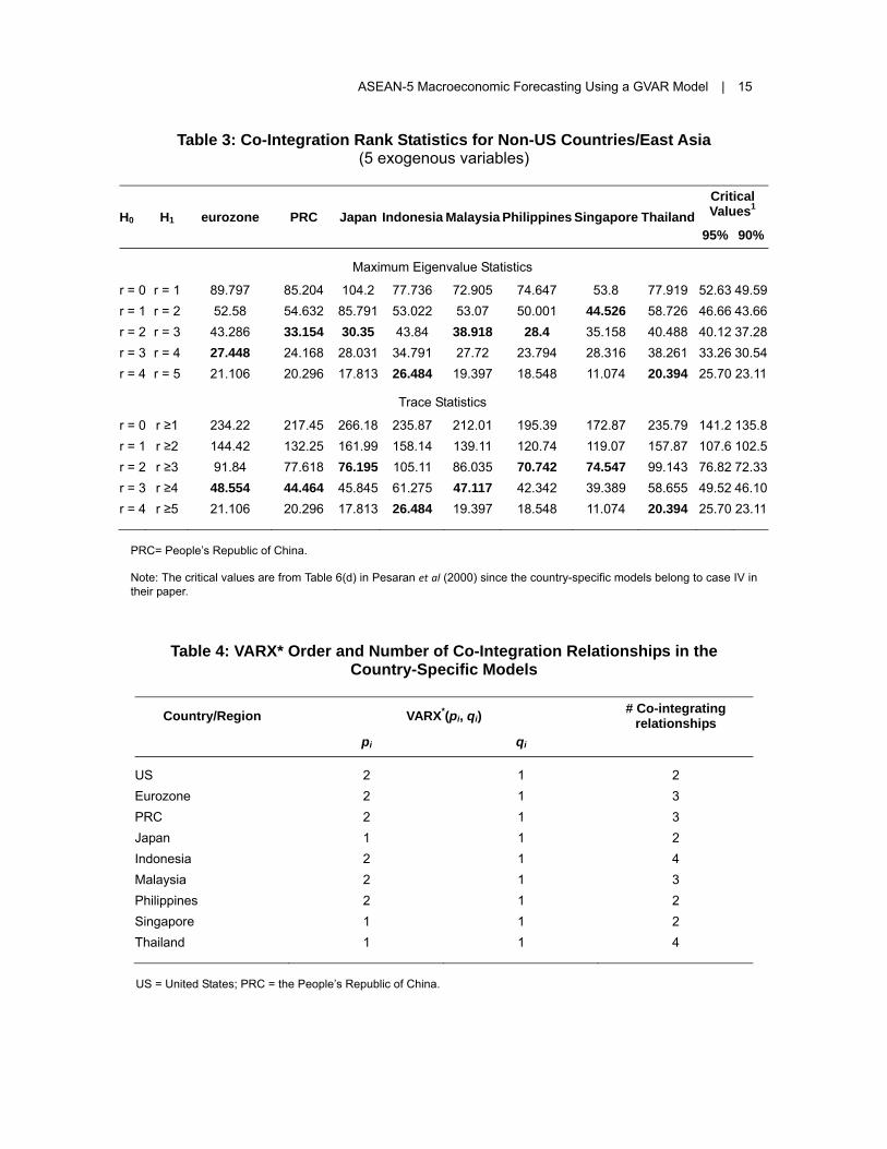
Table 3: Co-Integration Rank Statistics for Non-US Countries/East Asia (5 exogenous variables)

H0 H1 eurozone PRC Japan Indonesia Malaysia Philippines Singapore Thailand Critical Values1

95% 90%

Maximum Eigenvalue Statistics

r = 0 r = 1 89.797 85.204 104.2 77.736 72.905 74.647 53.8 77.919 52.63 49.59r = 1 r = 2 52.58 54.632 85.791 53.022 53.07 50.001 44.526 58.726 46.66 43.66r = 2 r = 3 43.286 33.154 30.35 43.84 38.918 28.4 35.158 40.488 40.12 37.28r = 3 r = 4 27.448 24.168 28.031 34.791 27.72 23.794 28.316 38.261 33.26 30.54r = 4 r = 5 21.106 20.296 17.813 26.484 19.397 18.548 11.074 20.394 25.70 23.11

Trace Statistics

r = 0 r ≥1 234.22 217.45 266.18 235.87 212.01 195.39 172.87 235.79 141.2 135.8r = 1 r ≥2 144.42 132.25 161.99 158.14 139.11 120.74 119.07 157.87 107.6 102.5r = 2 r ≥3 91.84 77.618 76.195 105.11 86.035 70.742 74.547 99.143 76.82 72.33r = 3 r ≥4 48.554 44.464 45.845 61.275 47.117 42.342 39.389 58.655 49.52 46.10r = 4 r ≥5 21.106 20.296 17.813 26.484 19.397 18.548 11.074 20.394 25.70 23.11

PRC= People’s Republic of China. Note: The critical values are from Table 6(d) in Pesaran et al (2000) since the country-specific models belong to case IV in their paper.

Table 4: VARX* Order and Number of Co-Integration Relationships in the Country-Specific Models

Country/Region VARX*(pi, qi) # Co-integrating

relationships pi qi

US 2 1 2 Eurozone 2 1 3 PRC 2 1 3 Japan 1 1 2 Indonesia 2 1 4 Malaysia 2 1 3 Philippines 2 1 2 Singapore 1 1 2 Thailand 1 1 4

US = United States; PRC = the People’s Republic of China.


Table 5: ADF-GLS Unit Root Test Statistics (based on MAIC order selection)

Domestic Variables US eurozone PRC Japan Indonesia Malaysia Philippines Singapore Thailand

y -0.578 -2.061 -1.135 -2.408 -2.477 -1.911 -1.312 -1.901 -1.683Δy -2.291 -4.953 -3.658 -4.970 -6.510 -3.913 -6.154 -5.946 -4.807Δ2y -13.486 -6.702 -12.503 -6.836 -14.041 -3.512 -12.004 -12.398 -10.203π -1.803 -2.524 -1.681 -0.882 -3.816 -1.803 -1.339 -3.261** -2.194Δπ -1.492* -8.978 -7.280 -1.140* -9.349 -4.606 -0.737* -10.524 -4.118Δ2π -8.949 -9.991 -11.397 -1.782* -16.547 -3.252 -0.505* -13.620 -7.752

r -2.506 -1.453 -2.156 -1.448 -2.363 -2.110 -2.345 -3.133** -2.806Δr -3.092 -3.186 -2.365 -3.306 -4.619 -8.238 -9.594 -4.691 -6.466Δ2r -9.643 -6.383 -4.142 -2.698 -10.240 -15.744 -6.406 -6.565 -10.561e -1.486 -0.976 -1.865 -1.794 -2.098 -1.902 -1.631 -1.136Δe -3.113 -4.165 -5.504 -3.757 -4.830 -5.055 -4.900 -4.456Δ2e -5.294 -14.656 -8.071 -14.778 -8.976 -10.426 -7.402 -10.387q -0.420 -1.137 -2.436 -2.699 -2.348 -2.492 -1.597 -2.637 -1.589Δq -4.353 -5.261 -5.667 -4.786 -4.513 -5.388 -6.248 -5.385 -6.858Δ2q -9.407 -9.002 -7.052 -5.903 -5.489 -8.110 -7.137 -8.367 -9.011y* -1.707 -1.233 -2.180 -1.448 -1.524 -1.767 -1.481 -2.276 -2.095Δy* -2.520 -2.891 -2.700 -2.848 -2.532 -2.264 -2.004* -3.525 -2.991Δ2y* -8.796 -10.458 -6.595 -10.416 -10.457 -8.666 -8.884 -6.957 -10.034π* -2.266 -2.225 -1.597 -2.421 -2.680 -3.101** -2.931 -3.852** -3.016Δπ* -9.633 -9.720 -1.630* -8.918 -8.532 -8.445 -8.527 -8.974 -9.211Δ2π* -14.208 -13.599 -5.168 -12.989 -12.901 -14.801 -12.879 -13.246 -16.163

r* -2.321 -1.297 -1.584 -1.394 -1.595 -1.253 -1.898 -1.413Δr* -2.739 -2.232 -1.601* -3.193 -2.565 -2.360 -2.035* -2.007*Δ2r* -6.945 -6.302 -3.151 -7.326 -6.987 -7.912 -4.014 -4.313e* -0.578 -0.567 -1.446 -0.880 -0.967 -0.917 -0.926 -1.289 -0.969Δe* -4.367 -6.839 -4.134 -3.248 -4.888 -5.159 -4.887 -3.465 -5.296Δ2e* -7.524 -12.662 -6.225 -11.284 -7.110 -8.533 -7.516 -11.267 -8.353q* -2.041 -1.869 -2.126 -2.490 -2.432 -2.383 -2.692 -2.516Δq* -2.077* -4.181 -2.084* -4.230 -4.424 -4.153 -4.678 -4.116Δ2q* -7.961 -6.148 -9.265 -9.131 -9.472 -9.020 -8.780 -9.319

p -1.698 -1.698 -1.698 -1.698 -1.698 -1.698 -1.698 -1.698 -1.698Δp -2.235 -2.235 -2.235 -2.235 -2.235 -2.235 -2.235 -2.235 -2.235Δ2p -9.173 -9.173 -9.173 -9.173 -9.173 -9.173 -9.173 -9.173 -9.173

US = United States; PRC = People’s Republic of China. Note: * denotes fail to reject the null hypothesis of unit root at 5% level. ** denotes reject the null hypothesis of unit root at 5% level.


Table 6: F-statistics for Testing the Weak Exogeneity of the Country-Specific Foreign Variables and Commodity Prices

Country Foreign variables

y* π* r* e* q* P

US F(2, 53) 0.72 3.86* 0.93

eurozone F(4, 54) 1.24 0.39 1.08 0.67 0.52

PRC F(3, 49) 0.56 1.90 0.87 1.01 0.95

Japan F(3, 55) 1.93 1.19 0.22 0.68 0.10

Indonesia F(3, 55) 0.82 0.23 1.15 0.49 0.14

Malaysia F(3, 55) 1.53 0.62 1.16 2.65 1.76

Philippines F(2, 50) 0.53 0.80 2.41 0.16 0.27

Singapore F(2, 56) 0.05 0.33 0.15 0.96 1.39

Thailand F(4, 54) 1.12 2.22 3.85* 0.87 2.03

US = United States; PRC = People’s Republic of China. Note: * denotes statistical significance at the 5% level.

Table 7: F-statistics for Tests of Residual Serial Correlation for Country-Specific VARX* Models

Country y π r e q p

US F(4, 55) 3.844* 1.294 0.572 1.400 3.201*

eurozone F(4, 57) 0.535 3.669* 2.677* 1.654 0.120

PRC F(4, 52) 1.053 0.268 1.623 0.143 3.513*

Japan F(4, 59) 1.443 2.153 2.152 2.798* 2.337

Indonesia F(4, 58) 1.146 0.685 1.169 1.345 0.544

Malaysia F(4, 58) 0.235 2.097 1.516 2.962* 0.787

Philippines F(4, 53) 0.363 0.815 1.588 0.932 3.688*

Singapore F(4, 59) 1.982 0.636 0.824 0.121 0.988

Thailand F(4, 57) 6.067* 2.122 2.486 1.776 2.633*

US = United States; PRC = People’s Republic of China. Note: * denotes statistical significance at the 5% level.


Table 8: Contemporaneous Effects of Foreign Variables on their Domestic Counterparts

Country Domestic variablesy π r q

US 0.488*** (0.15)

0.224*** (0.081)

eurozone 0.195 (0.148)

0.291*** (.0432)

0.451*** (0.157)

0.447*** (.1661612)

PRC -0.094 (0.177)

0.139 (0.335)

-0.156** (0.077)

-0.136 (0.286)

Japan 0.399* (0.223)

-0.144** (0.059)

-0.036 (0.054)

0.066 (0.179)

Indonesia -0.164 (0.541)

1.143 (0.770)

5.256** (2.574)

1.327** (0.162)

Malaysia 1.313*** (0.211)

0.938*** (0.257)

0.206 (0.151)

0.716*** (0.186)

Philippines 0.112 (0.250)

1.376*** (0.295)

2.761*** (0.923)

1.243*** (0.138)

Singapore 1.137*** (0.307)

0.038 (0.093)

0.127 (0.110)

0.925*** (0.119)

Thailand 1.015** (0.459)

0.310** (0.146)

3.766*** (0.502)

1.186*** (0.258)

US = United States; PRC = People’s Republic of China. Note: Newey-West HAC standard errors are given in parentheses. * denotes statistical significance at the 10% level, ** denotes statistical significance at the 5% level, and *** denotes statistical significance at the 1% level.

Table 9: Panel DM Statistics for GVAR Forecasts Relative to the Benchmark Model, 2009Q1–2009Q4

Benchmark Model

Real GDP Growth Rate Inflation Short-Term

Interest Rate Real Exchange

Rate Real Equity

Price

Country-specific VAR(2) -0.291 -0.210 -2.093* -0.480 -0.961

Country-specific VAR(2) with trend -0.253 -0.815 -2.199* -0.599 -1.113

Notes: * denotes statistical significance at the 5% level. A positive value of the panel DM statistic represents evidence against the GVAR forecasts.


AS

EA

N-5 M

acroeconomic Forecasting U

sing a GVA

R M

odel | 19

0 20 40 60 80-20

-10

0

10

20

Quarters

Indonesia Real GDP Growth Rate (%)

0 20 40 60 80-10

-5

0

5

10

Quarters

Malaysia Real GDP Growth Rate (%)

0 20 40 60 80-5

0

5

Quarters

Philippines Real GDP Growth Rate (%)

0 20 40 60 80-10

-5

0

5

10

Quarters

Singapore Real GDP Growth Rate (%)

0 20 40 60 80-10

-5

0

5

10

Quarters

Thailand Real GDP Growth Rate (%)

0 20 40 60 80-2

-1

0

1

2

Quarters

US Real GDP Growth Rate (%)

0 20 40 60 80-5

0

5

Quarters

EA Real GDP Growth Rate (%)

0 20 40 60 800

2

4

6

8

10

Quarters

PRC Real GDP Growth Rate (%)

0 20 40 60 80-5

0

5

Quarters

Japan Real GDP Growth Rate (%)

ForecastsActual data









Figure 1: One Quarter Ahead Forecasts for Real GDP Growth EA= Euro Area, PRC= People’s Republic of China.


20 | W

orking Paper Series on Regional E

conomic Integration N

o. 76

0 20 40 60 80-50

0

50

Quarters

Indonesia Inflation (%)

0 20 40 60 80-5

0

5

Quarters

Malaysia Inflation (%)

0 20 40 60 80-10

-5

0

5

10

Quarters

Philippines Inflation (%)

0 20 40 60 80-5

0

5

Quarters

Singapore Inflation (%)

0 20 40 60 80-5

0

5

Quarters

Thailand Inflation (%)

0 20 40 60 80-5

0

5

Quarters

US Inflation (%)

0 20 40 60 80-2

-1

0

1

2

Quarters

EA Inflation (%)

0 20 40 60 80-10

-5

0

5

10

Quarters

PRC Inflation (%)

0 20 40 60 80-2

-1

0

1

2

Quarters

Japan Inflation (%)










Figure 2: One Quarter Ahead Forecasts for Inflation

EA= Euro Area, PRC= People’s Republic of China.


AS

EA

N-5 M


sing a GVA

R M

odel | 21

Figure 3: One Quarter Ahead Forecasts for Short-Term Interest Rate


0 20 40 60 800

20

40

60

80

100

Quarters

Indonesia Short-Term Interest Rate (%)

0 20 40 60 800

2

4

6

8

10

Quarters

Malaysia Short-Term Interest Rate (%)

0 20 40 60 80-50

0

50

Quarters

Philippines Short-Term Interest Rate (%)

0 20 40 60 80-10

-5

0

5

10

Quarters

Singapore Short-Term Interest Rate (%)

0 20 40 60 800

10

20

30

40

Quarters

Thailand Short-Term Interest Rate (%)

0 20 40 60 80-10

-5

0

5

10

Quarters

US Short-Term Interest Rate (%)

0 20 40 60 80-20

-10

0

10

20

Quarters

EA Short-Term Interest Rate (%)

0 20 40 60 800

2

4

6

8

10

Quarters

PRC Short-Term Interest Rate (%)

0 20 40 60 80-10

-5

0

5

10

Quarters

Japan Short-Term Interest Rate (%)


Forecasts

Actual data









22 | W



o. 76

0 10 20 30 40 50 60 70 800

2

4x 10-5

Quarters

Indonesia Real Exchange Rate

0 10 20 30 40 50 60 70 802

4

6x 10-3

Quarters

Malaysia Real Exchange Rate

0 10 20 30 40 50 60 70 800

0.5

1x 10-3

Quarters

Philippines Real Exchange Rate

0 10 20 30 40 50 60 70 804

6

8x 10-3

Quarters

Singapore Real Exchange Rate

0 10 20 30 40 50 60 70 800

0.5

1x 10-3

Quarters

Thailand Real Exchange Rate

0 10 20 30 40 50 60 70 800

0.01

0.02

Quarters

EA Real Exchange Rate

0 10 20 30 40 50 60 70 800

2

4x 10-3

Quarters

PRC Real Exchange Rate

0 10 20 30 40 50 60 70 800.5

1

1.5x 10-4

Quarters

Japan Real Exchange Rate









Figure 4: One Quarter Ahead Forecasts for Real Exchange Rate EA= Euro Area, PRC= People’s Republic of China.


AS

EA

N-5 M


sing a GVA

R M

odel | 23

Figure 5: One Quarter Ahead Forecasts for Real Equity Prices EA= Euro Area, PRC= People’s Republic of China.

0 20 40 60 800

10

20

30

40

Quarters

Indonesia Real Equity Price

0 20 40 60 800

0.5

1

1.5

2

Quarters

Malaysia Real Equity Price

0 20 40 60 800

20

40

60

80

100

Quarters

Philippines Real Equity Price

0 20 40 60 800

0.5

1

1.5

2

Quarters

Singapore Real Equity Price

0 20 40 60 800

10

20

30

40

Quarters

Thailand Real Equity Price

0 20 40 60 800

0.5

1

1.5

2

Quarters

US Real Equity Price

0 20 40 60 800

1

2

3

4

5

Quarters

EA Real Equity Price

0 20 40 60 800

1

2

3

4

5

Quarters

PRC Real Equity Price

0 20 40 60 800

0.5

1

1.5

2

Quarters

Japan Real Equity Price






Forecasts

Actual data





24 | W



o. 76

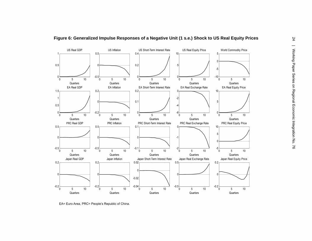
Figure 6: Generalized Impulse Responses of a Negative Unit (1 s.e.) Shock to US Real Equity Prices EA= Euro Area, PRC= People’s Republic of China.

0 5 100

0.5

1

Quarters

US Real GDP

0 5 10-0.5

0

0.5

Quarters

US Inflation

0 5 100

0.2

0.4

Quarters

US Short-Term Interest Rate

0 5 100

5

10

Quarters


0 5 10-10

-5

0

5

Quarters

World Commodity Price

0 5 100

0.5

1

1.5

Quarters

EA Real GDP

0 5 10-0.2

0

0.2

Quarters

EA Inflation

0 5 100

0.1

0.2

Quarters

EA Short-Term Interest Rate

0 5 10-6

-4

-2

0

Quarters


0 5 100

5

10

Quarters


0 5 10-0.5

0

0.5

Quarters

PRC Real GDP

0 5 10-0.5

0

0.5

Quarters

PRC Inflation

0 5 10-0.1

0

0.1

Quarters

PRC Short-Term Interest Rate

0 5 10-2

-1

0

Quarters


0 5 10-5

0

5

10

Quarters


0 5 10-0.2

0

0.2

Quarters

Japan Real GDP

0 5 10-0.2

0

0.2

Quarters

Japan Inflation

0 5 10-0.04

-0.02

0

0.02

Quarters

Japan Short-Term Interest Rate

0 5 10-0.5

0

0.5

Quarters


0 5 10-0.2

0

0.2

Quarters



AS

EA

N-5 M


sing a GVA

R M

odel | 25

0 5 10-0.04

-0.02

0

Quarters

Indonesia Real GDP

0 5 10-2

0

2

Quarters

Indonesia Inflation

0 5 10-0.2

0

0.2

Quarters

Indonesia Short-Term Interest Rate

0 5 100

5

10

Quarters


0 5 10-2

0

2

Quarters


0 5 100

0.5

1

Quarters

Malaysia Real GDP

0 5 10-1

0

1

Quarters

Malaysia Inflation

0 5 10-0.05

0

0.05

Quarters

Malaysia Short-Term Interest Rate

0 5 10-5

0

5

Quarters


0 5 10-0.5

0

0.5

Quarters


0 5 10-0.02

0

0.02

Quarters

Philippines Real GDP

0 5 10-1

0

1

Quarters

Philippines Inflation

0 5 100

0.2

0.4

Quarters

Philippines Short-Term Interest Rate

0 5 10-0.5

0

0.5

Quarters


0 5 100

2

4

Quarters


0 5 100

0.5

1

Quarters

Singapore Real GDP

0 5 10-0.1

0

0.1

Quarters

Singapore Inflation

0 5 10-0.05

0

0.05

Quarters

Singapore Short-Term Interest Rate

0 5 10-0.05

0

0.05

Quarters


0 5 10-0.5

0

0.5

Quarters


0 5 10-0.5

0

0.5

Quarters

Thailand Real GDP

0 5 10-0.5

0

0.5

Quarters

Thailand Inflation

0 5 10-0.5

0

0.5

Quarters

Thailand Short-Term Interest Rate

0 5 10-2

0

2

Quarters


0 5 10-20

0

20

Quarters


Figure 7: Generalized Impulse Responses of a Negative Unit (1 s.e.) Shock to US Real Equity Prices (cont.)


26 | W



o. 76

0 5 100

0.2

0.4

Quarters

US Real GDP

0 5 10-0.5

0

0.5

Quarters

US Inflation

0 5 100

0.2

0.4

Quarters


0 5 10-2

0

2

4

Quarters


0 5 10-5

0

5

Quarters


0 5 10-0.5

0

0.5

1

Quarters

EA Real GDP

0 5 10-0.05

0

0.05

Quarters

EA Inflation

0 5 100

0.1

0.2

Quarters


0 5 10-4

-2

0

2

Quarters


0 5 100

2

4

6

Quarters


0 5 10-0.5

0

0.5

Quarters

PRC Real GDP

0 5 10-0.2

0

0.2

Quarters

PRC Inflation

0 5 10-0.05

0

0.05

Quarters


0 5 10-1

-0.5

0

0.5

Quarters


0 5 10-5

0

5

10

Quarters


0 5 10-0.1

0

0.1

Quarters

Japan Real GDP

0 5 10-0.1

0

0.1

Quarters

Japan Inflation

0 5 10-0.04

-0.02

0

0.02

Quarters


0 5 10-0.2

0

0.2

Quarters


0 5 10-0.5

0

0.5

Quarters


Figure 8: Generalized Impulse Responses of a Positive Unit (1 s.e.) Shock to World Commodity Prices in the US Model



AS

EA

N-5 M


sing a GVA

R M

odel | 27

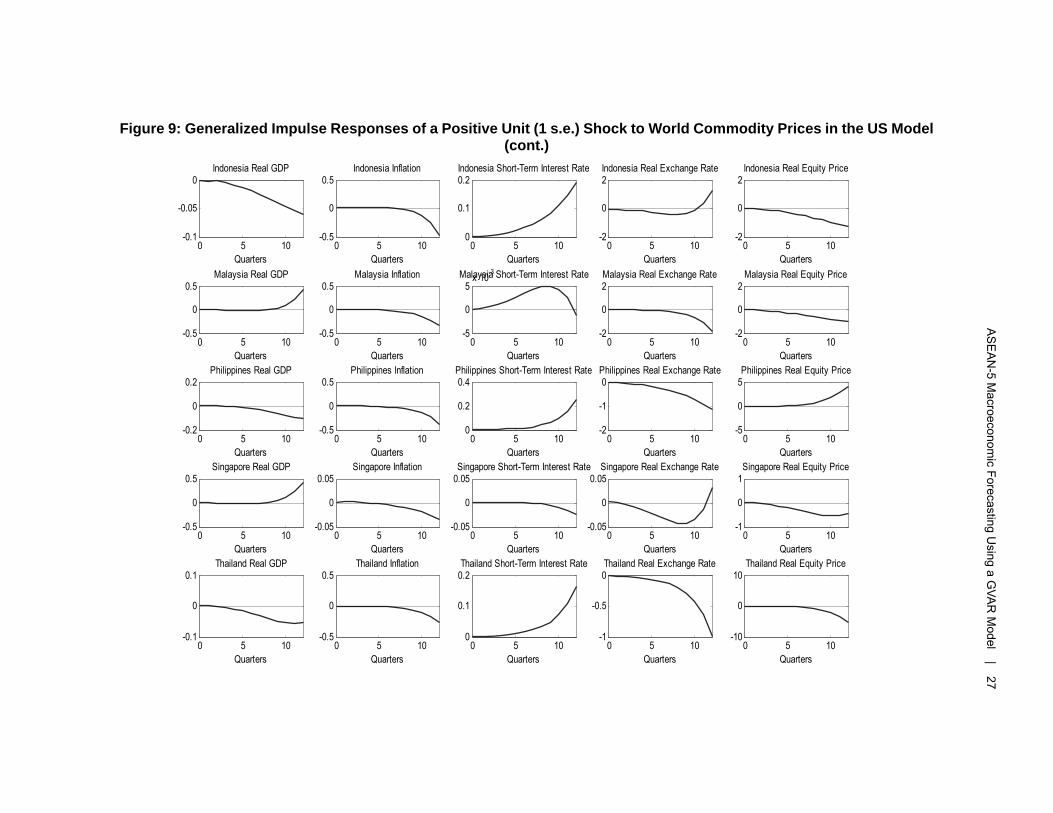
Figure 9: Generalized Impulse Responses of a Positive Unit (1 s.e.) Shock to World Commodity Prices in the US Model (cont.)

0 5 10-0.1

-0.05

0

Quarters

Indonesia Real GDP

0 5 10-0.5

0

0.5

Quarters

Indonesia Inflation

0 5 100

0.1

0.2

Quarters


0 5 10-2

0

2

Quarters


0 5 10-2

0

2

Quarters


0 5 10-0.5

0

0.5

Quarters

Malaysia Real GDP

0 5 10-0.5

0

0.5

Quarters

Malaysia Inflation

0 5 10-5

0

5x 10

-3

Quarters


0 5 10-2

0

2

Quarters


0 5 10-2

0

2

Quarters


0 5 10-0.2

0

0.2

Quarters


0 5 10-0.5

0

0.5

Quarters


0 5 100

0.2

0.4

Quarters


0 5 10-2

-1

0

Quarters


0 5 10-5

0

5

Quarters


0 5 10-0.5

0

0.5

Quarters

Singapore Real GDP

0 5 10-0.05

0

0.05

Quarters

Singapore Inflation

0 5 10-0.05

0

0.05

Quarters


0 5 10-0.05

0

0.05

Quarters


0 5 10-1

0

1

Quarters


0 5 10-0.1

0

0.1

Quarters

Thailand Real GDP

0 5 10-0.5

0

0.5

Quarters

Thailand Inflation

0 5 100

0.1

0.2

Quarters


0 5 10-1

-0.5

0

Quarters


0 5 10-10

0

10

Quarters



28 | W



o. 76

Figure 10: Generalized Impulse Responses of a Positive Unit (1 s.e.) to US Short-Term Interest Rates EA= Euro Area, PRC= People’s Republic of China.

0 5 100

0.2

0.4

Quarters

US Real GDP

0 5 10-0.5

0

0.5

Quarters

US Inflation

0 5 100

0.2

0.4

Quarters


0 5 100

2

4

6

Quarters


0 5 10-10

-5

0

5

Quarters


0 5 10-1

0

1

2

Quarters

EA Real GDP

0 5 10-0.1

0

0.1

Quarters

EA Inflation

0 5 100

0.1

0.2

Quarters


0 5 10-4

-2

0

2

Quarters


0 5 100

5

10

Quarters


0 5 100

0.2

0.4

Quarters

PRC Real GDP

0 5 10-0.5

0

0.5

Quarters

PRC Inflation

0 5 10-0.1

0

0.1

Quarters


0 5 10-2

-1

0

1

Quarters


0 5 10-5

0

5

10

Quarters


0 5 10-0.06

-0.04

-0.02

0

Quarters

Japan Real GDP

0 5 10-0.1

0

0.1

Quarters

Japan Inflation

0 5 10-0.04

-0.02

0

0.02

Quarters


0 5 10-0.5

0

0.5

Quarters


0 5 10-0.5

0

0.5

Quarters



AS

EA

N-5 M


sing a GVA

R M

odel | 29

0 5 10-0.02

-0.01

0

Quarters

Indonesia Real GDP

0 5 10-1

0

1

Quarters

Indonesia Inflation

0 5 100

0.1

0.2

Quarters


0 5 10-5

0

5

Quarters


0 5 10-1

0

1

Quarters


0 5 10-1

0

1

Quarters

Malaysia Real GDP

0 5 10-0.5

0

0.5

Quarters

Malaysia Inflation

0 5 10-0.02

0

0.02

Quarters


0 5 10-4

-2

0

Quarters


0 5 10-0.5

0

0.5

Quarters


0 5 10-0.05

0

0.05

Quarters


0 5 10-1

0

1

Quarters


0 5 100

0.2

0.4

Quarters


0 5 10-1

-0.5

0

Quarters


0 5 100

2

4

Quarters


0 5 10-1

0

1

Quarters

Singapore Real GDP

0 5 10-0.05

0

0.05

Quarters

Singapore Inflation

0 5 10-0.05

0

0.05

Quarters


0 5 10-0.1

0

0.1

Quarters


0 5 10-0.5

0

0.5

Quarters


0 5 10-0.1

0

0.1

Quarters

Thailand Real GDP

0 5 10-0.5

0

0.5

Quarters

Thailand Inflation

0 5 100

0.1

0.2

Quarters


0 5 10-2

-1

0

Quarters


0 5 10-10

0

10

Quarters


Figure 11: Generalized Impulse Responses of a Positive Unit (1 s.e.) Shock to US Short-Term Interest Rates (cont.)

30 |

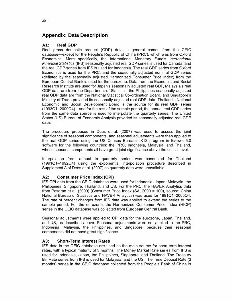
Appendix: Data Description A1: Real GDP Real gross domestic product (GDP) data in general comes from the CEIC database—except for the People’s Republic of China (PRC), which was from Oxford Economics. More specifically, the International Monetary Fund’s International Financial Statistics (IFS) seasonally adjusted real GDP series is used for Canada, and the real GDP series from IFS is used for Indonesia. The real GDP series from Oxford Economics is used for the PRC, and the seasonally adjusted nominal GDP series (deflated by the seasonally adjusted Harmonized Consumer Price Index) from the European Central Bank is used for the eurozone. Data from the Economic and Social Research Institute are used for Japan’s seasonally adjusted real GDP, Malaysia’s real GDP data are from the Department of Statistics, the Philippines seasonally adjusted real GDP data are from the National Statistical Co-ordination Board, and Singapore’s Ministry of Trade provided its seasonally adjusted real GDP data. Thailand’s National Economic and Social Development Board is the source for its real GDP series (1993Q1–2009Q4)—and for the rest of the sample period, the annual real GDP series from the same data source is used to interpolate the quarterly series. The United States (US) Bureau of Economic Analysis provided its seasonally adjusted real GDP data. The procedure proposed in Dees et al. (2007) was used to assess the joint significance of seasonal components, and seasonal adjustments were then applied to the real GDP series using the US Census Bureau’s X12 program in Eviews 5.0 software for the following countries: the PRC, Indonesia, Malaysia, and Thailand, whose seasonal components all have great joint significance above the critical level. Interpolation from annual to quarterly series was conducted for Thailand (1991Q1–1992Q4) using the exponential interpolation procedure described in Supplement A of Dees et al. (2007) as quarterly data were unavailable. A2: Consumer Price Index (CPI) IFS CPI data from the CEIC database were used for Indonesia, Japan, Malaysia, the Philippines, Singapore, Thailand, and US. For the PRC, the HAVER Analytics data from Pesaran et al. (2009) (Consumer Price Index (SA, 2000 = 100), source: China National Bureau of Statistics and HAVER Analytics) was used for 1991Q1–2005Q4. The rate of percent changes from IFS data was applied to extend the series to the sample period. For the eurozone, the Harmonized Consumer Price Index (HICP) series in the CEIC database was collected from European Central Bank. Seasonal adjustments were applied to CPI data for the eurozone, Japan, Thailand, and US, as described above. Seasonal adjustments were not applied to the PRC, Indonesia, Malaysia, the Philippines, and Singapore, because their seasonal components did not have great significance.

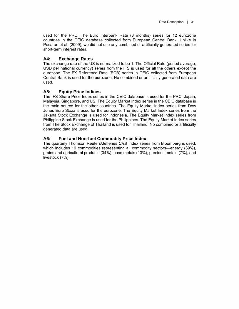
A3: Short-Term Interest Rates IFS data in the CEIC database are used as the main source for short-term interest rates, with a typical maturity of 3 months. The Money Market Rate series from IFS is used for Indonesia, Japan, the Philippines, Singapore, and Thailand. The Treasury Bill Rate series from IFS is used for Malaysia, and the US. The Time Deposit Rate (3 months) series in the CEIC database collected from the People’s Bank of China is

Data Description | 31

used for the PRC. The Euro Interbank Rate (3 months) series for 12 eurozone countries in the CEIC database collected from European Central Bank. Unlike in Pesaran et al. (2009), we did not use any combined or artificially generated series for short-term interest rates. A4: Exchange Rates The exchange rate of the US is normalized to be 1. The Official Rate (period average, USD per national currency) series from the IFS is used for all the others except the eurozone. The FX Reference Rate (ECB) series in CEIC collected from European Central Bank is used for the eurozone. No combined or artificially generated data are used. A5: Equity Price Indices The IFS Share Price Index series in the CEIC database is used for the PRC, Japan, Malaysia, Singapore, and US. The Equity Market Index series in the CEIC database is the main source for the other countries. The Equity Market Index series from Dow Jones Euro Stoxx is used for the eurozone. The Equity Market Index series from the Jakarta Stock Exchange is used for Indonesia. The Equity Market Index series from Philippine Stock Exchange is used for the Philippines. The Equity Market Index series from The Stock Exchange of Thailand is used for Thailand. No combined or artificially generated data are used. A6: Fuel and Non-fuel Commodity Price Index The quarterly Thomson Reuters/Jefferies CRB Index series from Bloomberg is used, which includes 19 commodities representing all commodity sectors—energy (39%), grains and agricultural products (34%), base metals (13%), precious metals,(7%), and livestock (7%).

32 |

References S. Dees, F. di Mauro, M.H. Pesaran, and L.V. Smith. 2007. Exploring the International

Linkages in the Euro Area: A Global VAR Analysis. Journal of Applied Econometrics. 22 (1). pp. 1–38.

G. Elliot, T. J. Rothenberg, and J. H. Stock. 1996. Efficient Tests for an Autoregressive

Unit Root. Econometrica. 64 (4). pp. 813–836. S. Johansen. 1988. Statistical Analysis of Cointegration Vectors. Journal of Economic

Dynamics and Control. 12. pp. 231–254. ———. 1992. Cointegration in Partial Systems and the Efficiency of Single-equation

Analysis. Journal of Econometrics. 52 (3). pp. 389–402. G. Koop, M. H. Pesaran, and S. M. Potter. 1996. Impulse Response Analysis in

Nonlinear Multivariate Models. Journal of Econometrics. 74 (1). pp. 119–147. M. H. Pesaran, T. Schuermann, and L.V. Smith. 2009. Forecasting Economic and

Financial Variables with Global VARs. International Journal of Forecasting. 25 (4). pp. 642–675.

M. H. Pesaran, T. Schuermann, and S. M. Weiner. 2004. Modeling Regional

Interdependencies Using a Global Error-correcting Macroeconometric Model. Journal of Business & Economic Statistics. 22 (2). pp. 129–162.

M. H. Pesaran, and Y. Shin. 2002. Long-run Structural Modeling. Econometric

Reviews. 21 (1). pp. 49–87. M. H. Pesaran, Y. Shin, and R. J. Smith. 2000. Structural Analysis of Vector Error

Correction Models with Exogenous I(1) Variables. Journal of Econometrics. 97 (2). pp. 293–343.

P. C. B. Phillips. 1995. Fully Modified Least Squares and Vector Autoregression.

Econometrica. 63 (5). pp. 1023–78.

| 33

ADB Working Paper Series on Regional Economic Integration*

1. “The ASEAN Economic Community and the European Experience” by

Michael G. Plummer

2. “Economic Integration in East Asia: Trends, Prospects, and a Possible Roadmap” by Pradumna B. Rana

3. “Central Asia after Fifteen Years of Transition: Growth, Regional Cooperation, and Policy Choices” by Malcolm Dowling and Ganeshan Wignaraja

4. “Global Imbalances and the Asian Economies: Implications for Regional Cooperation” by Barry Eichengreen

5. “Toward Win-Win Regionalism in Asia: Issues and Challenges in Forming Efficient Trade Agreements” by Michael G. Plummer

6. “Liberalizing Cross-Border Capital Flows: How Effective Are Institutional Arrangements against Crisis in Southeast Asia” by Alfred Steinherr, Alessandro Cisotta, Erik Klär, and Kenan Šehović

7. “Managing the Noodle Bowl: The Fragility of East Asian Regionalism” by Richard E. Baldwin

8. “Measuring Regional Market Integration in Developing Asia: a Dynamic Factor Error Correction Model (DF-ECM) Approach” by Duo Qin, Marie Anne Cagas, Geoffrey Ducanes, Nedelyn Magtibay-Ramos, and Pilipinas F. Quising

9. “The Post-Crisis Sequencing of Economic Integration in Asia: Trade as a Complement to a Monetary Future” by Michael G. Plummer and Ganeshan Wignaraja

10. “Trade Intensity and Business Cycle Synchronization: The Case of East Asia” by Pradumna B. Rana

11. “Inequality and Growth Revisited” by Robert J. Barro

12. “Securitization in East Asia” by Paul Lejot, Douglas Arner, and Lotte Schou-Zibell

13. “Patterns and Determinants of Cross-border Financial Asset Holdings in East Asia” by Jong-Wha Lee

14. “Regionalism as an Engine of Multilateralism: A Case for a Single East Asian FTA” by Masahiro Kawai and Ganeshan Wignaraja

15. “The Impact of Capital Inflows on Emerging East Asian Economies: Is Too Much Money Chasing Too Little Good?” by Soyoung Kim and Doo Yong Yang

34 |

16. “Emerging East Asian Banking Systems Ten Years after the 1997/98 Crisis” by Charles Adams

17. “Real and Financial Integration in East Asia” by Soyoung Kim and Jong-Wha Lee

18. “Global Financial Turmoil: Impact and Challenges for Asia’s Financial Systems” by Jong-Wha Lee and Cyn-Young Park

19. “Cambodia’s Persistent Dollarization: Causes and Policy Options” by Jayant Menon

20. “Welfare Implications of International Financial Integration” by Jong-Wha Lee and Kwanho Shin

21. “Is the ASEAN-Korea Free Trade Area (AKFTA) an Optimal Free Trade Area?” by Donghyun Park, Innwon Park, and Gemma Esther B. Estrada

22. “India’s Bond Market—Developments and Challenges Ahead” by Stephen Wells and Lotte Schou- Zibell

23. “Commodity Prices and Monetary Policy in Emerging East Asia” by Hsiao Chink Tang

24. “Does Trade Integration Contribute to Peace?” by Jong-Wha Lee and Ju Hyun Pyun

25. “Aging in Asia: Trends, Impacts, and Responses” by Jayant Menon and Anna Melendez-Nakamura

26. “Re-considering Asian Financial Regionalism in the 1990s” by Shintaro Hamanaka

27. “Managing Success in Viet Nam: Macroeconomic Consequences of Large Capital Inflows with Limited Policy Tools” by Jayant Menon

28. “The Building Block versus Stumbling Block Debate of Regionalism: From the Perspective of Service Trade Liberalization in Asia” by Shintaro Hamanaka

29. “East Asian and European Economic Integration: A Comparative Analysis” by Giovanni Capannelli and Carlo Filippini

30. “Promoting Trade and Investment in India’s Northeastern Region” by M. Govinda Rao

31. “Emerging Asia: Decoupling or Recoupling” by Soyoung Kim, Jong-Wha Lee, and Cyn-Young Park

32. “India’s Role in South Asia Trade and Investment Integration” by Rajiv Kumar and Manjeeta Singh

| 35

33. “Developing Indicators for Regional Economic Integration and Cooperation” by Giovanni Capannelli, Jong-Wha Lee, and Peter Petri

34. “Beyond the Crisis: Financial Regulatory Reform in Emerging Asia” by Chee Sung Lee and Cyn-Young Park

35. “Regional Economic Impacts of Cross-Border Infrastructure: A General Equilibrium Application to Thailand and Lao PDR” by Peter Warr, Jayant Menon, and Arief Anshory Yusuf

36. “Exchange Rate Regimes in the Asia-Pacific Region and the Global Financial Crisis” by Warwick J. McKibbin and Waranya Pim Chanthapun

37. “Roads for Asian Integration: Measuring ADB's Contribution to the Asian Highway Network” by Srinivasa Madhur, Ganeshan Wignaraja, and Peter Darjes

38. “The Financial Crisis and Money Markets in Emerging Asia” by Robert Rigg and Lotte Schou-Zibell

39. “Complements or Substitutes? Preferential and Multilateral Trade Liberalization at the Sectoral Level” by Mitsuyo Ando, Antoni Estevadeordal, and Christian Volpe Martincus

40. “Regulatory Reforms for Improving the Business Environment in Selected Asian Economies—How Monitoring and Comparative Benchmarking can Provide Incentive for Reform” by Lotte Schou-Zibell and Srinivasa Madhur

41. “Global Production Sharing, Trade Patterns, and Determinants of Trade Flows in East Asia” by Prema-chandra Athukorala and Jayant Menon

42. “Regionalism Cycle in Asia (-Pacific): A Game Theory Approach to the Rise and Fall of Asian Regional Institutions” by Shintaro Hamanaka

43. “A Macroprudential Framework for Monitoring and Examining Financial Soundness” by Lotte Schou-Zibell, Jose Ramon Albert, and Lei Lei Song

44. “A Macroprudential Framework for the Early Detection of Banking Problems in Emerging Economies” by Claudio Loser, Miguel Kiguel, and David Mermelstein

45. “The 2008 Financial Crisis and Potential Output in Asia: Impact and Policy Implications” by Cyn-Young Park, Ruperto Majuca, and Josef Yap

46. “Do Hub-and-Spoke Free Trade Agreements Increase Trade? A Panel Data Analysis” by Jung Hur, Joseph Alba, and Donghyun Park

47. “Does a Leapfrogging Growth Strategy Raise Growth Rate? Some International Evidence” by Zhi Wang, Shang-Jin Wei, and Anna Wong

48. “Crises in Asia: Recovery and Policy Responses” by Kiseok Hong and Hsiao Chink Tang

36 |

49. “A New Multi-Dimensional Framework for Analyzing Regional Integration: Regional Integration Evaluation (RIE) Methodology” by Donghyun Park and Mario Arturo Ruiz Estrada

50. “Regional Surveillance for East Asia: How Can It Be Designed to Complement Global Surveillance?” by Shinji Takagi

51. “Poverty Impacts of Government Expenditure from Natural Resource Revenues” by Peter Warr, Jayant Menon, and Arief Anshory Yusuf

52. “Methods for Ex Ante Economic Evaluation of Free Trade Agreements” by David Cheong

53. “The Role of Membership Rules in Regional Organizations” by Judith Kelley

54. “The Political Economy of Regional Cooperation in South Asia” by V.V. Desai

55. “Trade Facilitation Measures under Free Trade Agreements: Are They Discriminatory against Non-Members?” by Shintaro Hamanaka, Aiken Tafgar, and Dorothea Lazaro

56. “Production Networks and Trade Patterns in East Asia: Regionalization or Globalization?” by Prema-chandra Athukorala

57. “Global Financial Regulatory Reforms: Implications for Developing Asia” by Douglas W. Arner and Cyn-Young Park

58. “Asia’s Contribution to Global Rebalancing” by Charles Adams, Hoe Yun Jeong, and Cyn-Young Park

59. “Methods for Ex Post Economic Evaluation of Free Trade Agreements” by David Cheong

60. “Responding to the Global Financial and Economic Crisis: Meeting the Challenges in Asia” by Douglas W. Arner and Lotte Schou-Zibell

61. “Shaping New Regionalism in the Pacific Islands: Back to the Future?” by Satish Chand

62. “Organizing the Wider East Asia Region” by Christopher M. Dent

63. “Labour and Grassroots Civic Interests In Regional Institutions” by Helen E.S. Nesadurai

64. “Institutional Design of Regional Integration: Balancing Delegation and Representation” by Simon Hix

65. “Regional Judicial Institutions and Economic Cooperation: Lessons for Asia?” by Erik Voeten

| 37

66. “The Awakening Chinese Economy: Macro and Terms of. Trade Impacts on 10 Major Asia-Pacific Countries” by Yin Hua Mai, Philip Adams, Peter Dixon, and Jayant Menon

67. “Institutional Parameters of a Region-Wide Economic Agreement in Asia: Examination of Trans-Pacific Partnership and ASEAN+α Free Trade Agreement Approaches” by Shintaro Hamanaka

68. “Evolving Asian Power Balances and Alternate Conceptions for Building Regional Institutions” by Yong Wang

69. “ASEAN Economic Integration: Features, Fulfillments, Failures, and the Future” by Hal Hill and Jayant Menon

70. “Changing Impact of Fiscal Policy on Selected ASEAN Countries” by Hsiao Chink Tang, Philip Liu, and Eddie C. Cheung

71. “The Organizational Architecture of the Asia-Pacific: Insights from the New Institutionalism” by Stephan Haggard

72. “The Impact of Monetary Policy on Financial Markets in Small Open Economies: More or Less Effective During the Global Financial Crisis?” by Steven Pennings, Arief Ramayandi, and Hsiao Chink Tang

73. “What do Asian Countries Want the Seat at the High Table for? G20 as a New Global Economic Governance Forum and the Role of Asia” by Yoon Je Cho

74. “Asia’s Strategic Participation in the Group of 20 for Global Economic Governance Reform: From the Perspective of International Trade” by Taeho Bark and Moonsung Kang

75. “ASEAN’s Free Trade Agreements with the People’s Republic of China, Japan, and the Republic of Korea: A Qualitative and Quantitative Analysis” by Gemma Estrada, Donghyun Park, Innwon Park, and Soonchan Park

* These papers can be downloaded from: (ARIC) http://aric.adb.org/reipapers/ or (ADB) www.adb.org/publications/category.asp?id=2805

ASEAN-5 Macroeconomic Forecasting Using a GVAR Model

This paper uses a global vector autoregressive (GVAR) model to forecast real GDP, inflation, short-term interest rates, real exchange rates, and real equity prices for five Southeast Asian countries. The key advantage of the GVAR model is that it allows us to incorporate the global interdependencies in the world economy into our model. This is especially important when we are modelling open economies such as the five Southeast Asian countries. We find that the forecasts from our GVAR model tend to outperform forecasts based on country-specific models.

About the Asian Development Bank

ADB’s vision is an Asia and Pacific region free of poverty. Its mission is to help its developing member countries reduce poverty and improve the quality of life of their people. Despitethe region’s many successes, it remains home to two-thirds of the world’s poor: 1.8 billionpeople who live on less than $2 a day, with 903 million struggling on less than $1.25 a day.ADB is committed to reducing poverty through inclusive economic growth, environmentallysustainable growth, and regional integration.

Based in Manila, ADB is owned by 67 members, including 48 from the region. Its main instruments for helping its developing member countries are policy dialogue, loans, equity investments, guarantees, grants, and technical assistance.

Asian Development Bank6 ADB Avenue, Mandaluyong City1550 Metro Manila, Philippineswww.adb.org/povertyPublication Stock No. WPS113351 Printed in the Philippines

Documents

ADB Working Paper Series on Regional Economic Integration · PDF fileADB Working Paper Series on Regional Economic Integration ... Macroeconomic Forecasting, Global vector ... to develop