Adaptive Optics Model

Anita Enmark

Lund Observatory

Outline

• Adaptive Optics Model• Current Work

Generalization Model Improvment Parallelization

Euro50 Model OverviewSCAO on a NGS

DM3169

Actuators

Adaptive Optics ModelTest Vehicle for AO Design together with ELT

Atmosphere

Controller

ReconstructionWavefront

sensorDeformable

mirror

• SCAO / NGS• Geometrical or Fresnel Propagation• SVD• Various influence functions and geometries• DM1: 2nd order systems for every actuator• Delay/non-linearities from WFS• Geometrical or physical model of SH-WFS

Current Work

• Generalization

• Improved adaptive optics model

• Parallelization

Generalization and improvment

• Adaptive optics model tested for VTT

• Improved model (atmosphere, noise etc)

WFS-lenslet CCD

Tip/Tilt Mirror

Deformable Mirror

LP-filter

Reconstruction and command

Discrete PID regulator

Pupil Plane

Photon noise

Source OPD

Actuator diff. commands

Actuator diff. commandDiscrete PID regulatorLP-filter

Actuator command

Actuator command

AD-Converter

Movie of VTT model with modes 1,2 (tip/tilt) and 30-35 set to

zero

Parallelization

Simulation environment for first order model Beowulf cluster with Matlab+MatlabWS

Memory capacity limiting factorFull matrix with DM influence function 6GBfor 3169 actuators64 bit Matlab needed– more primary memoryParts of code too slowSimple first order model takes many days/secNetwork too slow

Currently evaluating other simulation environments

Cluster – LUNARC, Lund

Shared memory - Galway, Ireland

ODE Multirate Solvers for Systems with Mixed Dynamics

1 million State Variables

Fast SubsystemSlow Subsystem

• Modern work on multi-rate solvers (eg. Anne Kværnø et al)• Andrus: Mixed 4th order Runge-Kutta• Simpler multirate solvers with extra/interpolation• Execution time reduction 5-10x

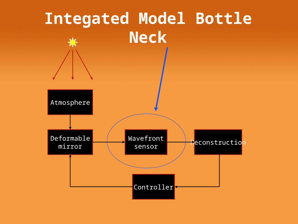
Integated Model Bottle Neck

Atmosphere

Controller

ReconstructionWavefront

sensorDeformable

mirror

Main drivers for execution time:

• One image for each subaperture -> For every subaperture: exponential and 2D IFFT

• Must give FOV as close to nominal as possible -> interpolation of wavefront

Shack-Hartman Wavefont Sensor Model

),( yx

),(2

exp),(),( 1 yxiyxuFI yx

),( yx1F

Every subaperture is propagated to the image plane with Fraunhofer propagation. The image of the subaperture wavefront in angular coordinates is then

where u(x,y) is the complex amplitude of the wavefront in the spatial coordinate system (x,y) and is the wavefront phase.

denotes the inverse Fourier transform.

Image formation

2

=> exponential and IFFT

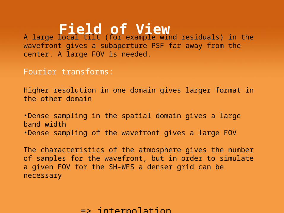
A large local tilt (for example wind residuals) in the wavefront gives a subaperture PSF far away from the center. A large FOV is needed.

Fourier transforms:

Higher resolution in one domain gives larger format in the other domain

•Dense sampling in the spatial domain gives a large band width•Dense sampling of the wavefront gives a large FOV

The characteristics of the atmosphere gives the number of samples for the wavefront, but in order to simulate a given FOV for the SH-WFS a denser grid can be necessary

=> interpolation

Field of View

Good News:Both have outer loops with an independent variable=>Suitable for parallelization.

Bad News:Matlabs parallel computing tools not good for our needs. MatlabWS not ported to shared memory machine. New C-code needed.

More good news:The bottle necks are within the same Matlab subfunction, only a limited part of the model must be coded in C. This gives fast execution, but keeps good structure.

Model groves with more sensors – can be parallelized

Impact on AO-model

0.5 1 1.5 2 2.5 3 3.5 4 4.5

0.5

1

1.5

2

2.5

3

3.5

4

4.50.5 1 1.5 2 2.5 3 3.5 4 4.5

0.5

1

1.5

2

2.5

3

3.5

4

4.5

50 100 150 200

50

100

150

200

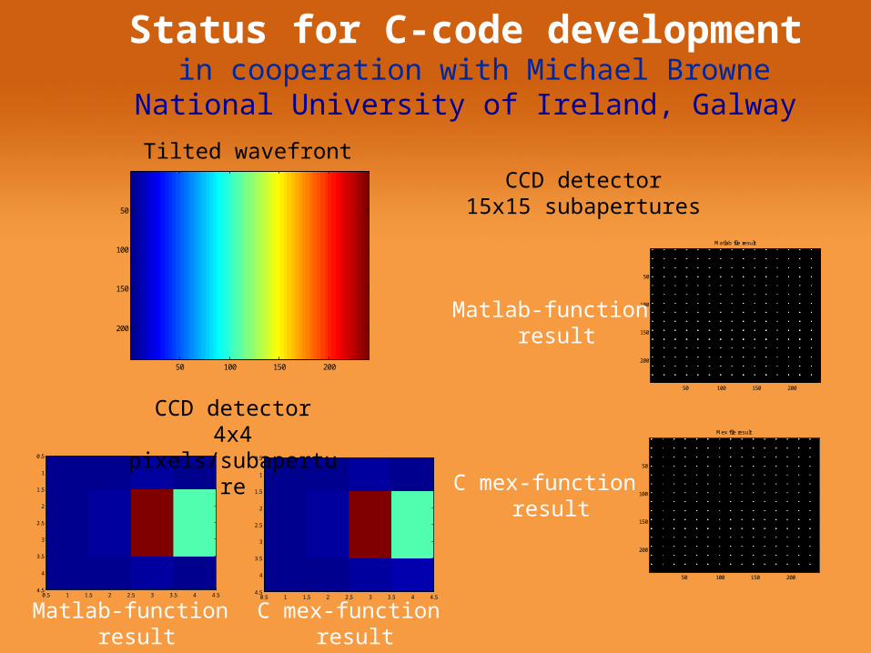
Mex file result

50 100 150 200

50

100

150

200

Matlab file result

50 100 150 200

50

100

150

200

Tilted wavefront

CCD detector4x4 pixels/subaperture

C mex-function result

Matlab-function result

C mex-function result

Matlab-function result

CCD detector15x15 subapertures

Status for C-code development in cooperation with Michael Browne

National University of Ireland, Galway

Test results for one call to WFS

Matlab on one CPU machine ~ 100 sec

Sequential C-code on the same machine ~ 14 sec

Sequential C-code on Itanium machine ~ 4 sec

Expected for multi-processor Itanium ~ 0.5 sec

Integrated Modeling

Conclusions

• A full Euro50 model with AO in place

• Generalization work in progress

• AO model improved

• Parallelization in progress – faster network and more memory needed – under test

• First tests promising

Full first order model simulation

Atmosphere correction