ADAPTIVE FINITE ELEMENTS FOR ELLIPTIC OPTIMIZATION ... · Heidelberg, Germany ([email protected]). This author’s research was sup- ported by the DFG priority

Copyright © by SIAM. Unauthorized reproduction of this article is prohibited.

SIAM J. CONTROL OPTIM. c© 2008 Society for Industrial and Applied MathematicsVol. 47, No. 1, pp. 509–534

ADAPTIVE FINITE ELEMENTS FOR ELLIPTIC OPTIMIZATIONPROBLEMS WITH CONTROL CONSTRAINTS∗

B. VEXLER† AND W. WOLLNER‡

Abstract. In this paper we develop a posteriori error estimates for finite element discretization ofelliptic optimization problems with pointwise inequality constraints on the control variable. We deriveerror estimators for assessing the discretization error with respect to the cost functional as well as withrespect to a given quantity of interest. These error estimators provide quantitative information aboutthe discretization error and guide an adaptive mesh refinement algorithm allowing for substantialsaving in degrees of freedom. The behavior of the method is demonstrated on numerical examples.

Key words. mesh adaptivity, optimal control, a posteriori error estimates, finite elementmethod, quantity of interest, pointwise inequality constraints

AMS subject classifications. 65N50, 65N30, 65K10

DOI. 10.1137/070683416

1. Introduction. In this paper we develop a posteriori error estimates for fi-nite element approximations of optimization problems governed by elliptic partialdifferential equations. We discuss this question in a general manner, including theconsideration of optimal control and parameter identification problems with controlconstraints given through a closed convex admissible set. The derived error estimateshave the goal of guiding an adaptive mesh refinement algorithm for finding economicalmeshes for the optimization problem under consideration.

The use of adaptive techniques based on a posteriori error estimation is wellaccepted in the context of finite element discretization of partial differential equations;see, e.g., [6, 13, 35]. To our knowledge there are only a few results published onadaptive finite elements for optimization problems; see [2, 17, 20, 23, 25, 27, 4, 7, 8, 30].

In articles [17, 20, 23, 25, 27] the authors provide a posteriori error estimates forelliptic optimal control problems with distributed or Neumann control subject to boxconstraints. These estimates assess the error in the control, state, and the adjointvariable with respect to the natural norms of the corresponding spaces. In [2] anotherapproach for the estimation of the error with respect to the norm of the control spaceis presented. In [17] convergence of an adaptive algorithm for a control constrainedoptimal control problem is shown.

However, in many applications, the error in global norms does not provide auseful error bound for the error in the quantity of physical interest. The a posteri-ori estimators derived in this paper grant access to the error with respect to givenfunctionals.

∗Received by the editors February 22, 2007; accepted for publication (in revised form) August 10,2007; published electronically February 1, 2008.

http://www.siam.org/journals/sicon/47-1/68341.html†Johann Radon Institute for Computational and Applied Mathematics (RICAM), Austrian

Academy of Sciences, Altenberger Straße 69, 4040 Linz, Austria ([email protected]). Thisauthor’s research was partially supported by the Austrian Science Fund FWF project P18971-N18“Numerical analysis and discretization strategies for optimal control problems with singularities.”

‡Institut fur Angewandte Mathematik, Ruprecht-Karls-Universitat Heidelberg, INF 294, 69120Heidelberg, Germany ([email protected]). This author’s research was sup-ported by the DFG priority program “Optimization with Partial Differential Equations.”

509


510 B. VEXLER AND W. WOLLNER

In [4, 6] the authors present a general concept for a posteriori estimation of thediscretization error with respect to the cost functional in the context of optimal controlproblems. In articles [7, 8] the authors have extended this approach to the estimationof the discretization error with respect to an arbitrary functional depending on boththe control and the state variable, so-called quantity of interest. This allowed, amongother things, the treatment of parameter identification and model calibration prob-lems. However, in all these publications, the control variable was searched for in aHilbert space Q without additional (inequality) constraints. Therefore the main con-tribution of this work is the extension of these techniques to the case of optimizationproblems with additional control constraints given through a closed convex admissibleset Qad ⊂ Q. In the majority of practical cases this admissible set is described byinequality control constraints of box type q− ≤ q(x) ≤ q+. Therefore we will concen-trate on this case, although our techniques may also be extended to the considerationof more general admissible sets Qad.

In this paper we consider optimization problems governed by (nonlinear) partialdifferential equations. The aim is to minimize a given cost functional J(q, u) whichdepends on the state variable u ∈ V and the control variable q ∈ Q, with Hilbertspaces V and Q. These variables have to satisfy the state equation

(1.1) A(q, u) = f,

where A denotes a (nonlinear) differential operator and f represents the given data.The optimization problem is then formulated as follows:

(1.2)

{Minimize J(q, u), u ∈ V, q ∈ Qad,

A(q, u) = f.

Constraints on the control are incorporated via the definition of the closed and convexset Qad representing the set of admissible controls.

For numerical treatment this infinite dimensional optimization problem is dis-cretized in virtue of finite element methods; see the discussion in section 3. Let thesolution to the discretized problem be denoted by (qh, uh). Our aim is to derive aposteriori error estimates for the error between the solutions to the continuous andthe discrete problem. A crucial point for our error analysis is the choice of a quantity,which describes the goal of the computation. If this quantity coincides with the costfunctional, we have to estimate the error

J(q, u) − J(qh, uh).

In a more general case, we suppose I : Q×V → R to be a given functional describingthe quantity of interest. Then the error to be estimated is

I(q, u) − I(qh, uh).

The consideration of quantities of interest is important, for instance, in the contextof parameter identification and model calibration problem; see [8] for an applicationof this concept to an optimization problem from computational fluid dynamics.

To the authors’ knowledge this is the first article providing a posteriori errorestimates with respect to a given functional for optimization problems with partialdifferential equations and subject to control constraints.

The paper is organized as follows. In the next section we describe the optimizationproblem under consideration, discuss necessary optimality conditions, and sketch the


ADAPTIVITY FOR OPTIMAL CONTROL 511

solution algorithm on the continuous level. In section 3 we describe the discretizationof the optimization problem in virtue of finite element methods. Section 4 is devotedto a posteriori error estimation. In sections 4.1 and 4.2 we derive two different errorestimates for the error with respect to the cost functional J . The first error estimator isbased on the optimality system involving a variational inequality, whereas the secondone exploits Lagrange multipliers for the treatment of inequality constraints. Dueto the fact that the optimal control q is not expected to be sufficiently smooth (dueto inequality constraints), the approximation of (interpolation) weights involved inthe error estimator cannot be treated in a usual way. To overcome this difficulty weexploit the projection formula (2.9) from the optimality conditions and propose anapproximation on the (interpolation) weights using a postprocessing step (4.7), whichis motivated by the considerations in [31]. In section 4.3 we provide an error estimatorwith respect to a given quantity of interest. To this end we utilize an additional (dual)linear-quadratic optimal control problem describing the sensitivity with respect to thequantity of interest. In the last section we present numerical examples to illustratethe behavior of our method.

2. Optimization problem. In this section we give a precise formulation of theoptimization problem under consideration and describe necessary optimality condi-tions and the solution algorithm.

In order to deal with different types of optimization problems simultaneously, weseek the control variable q in the Hilbert space Q = L2(ω) with scalar product (·, ·)and norm ‖·‖. Typically, ω is a subset of the computational domain Ω or a subsetof its boundary ∂Ω. The case of finite dimensional controls is realized by choosingω = {1, 2, . . . , n} resulting in Q ∼= R

n.Throughout this paper we suppose that the state equation (1.1) for u ∈ V is given

in a weak form:

(2.1) a(q, u)(ϕ) = f(ϕ) ∀ϕ ∈ V,

where a : Q×V ×V → R is a four times directional differentiable form which is linearin the third argument and f is in the dual space V ′. A possible choice for this spaceis V = H1(Ω), or V = H1

0 (Ω), or a direct product of such spaces. In the presence ofinhomogeneous Dirichlet boundary conditions, one seeks the state variable u in u+V ,where u represents the boundary data. However, for clarity of notation, we assumethroughout that u = 0.

Remark 2.1. Throughout this paper we use two pairs of parentheses after aform to indicate that the form is linear in all variables enclosed by the second pair ofparentheses, as seen in (2.1) for a(·, ·)(·).

The cost function is given by

(2.2) J(q, u) = J1(u) +α

2‖q‖2 ,

where J1 is a four times directionally differentiable operator on V and α > 0. Let theadmissible set Qad be given through box constraints on q, i.e.,

(2.3) Qad = {q ∈ Q | q− ≤ q(x) ≤ q+ a.e. on ω},

with bounds q−, q+ ∈ R ∪ {±∞} and q− < q+.Now we are able to formulate the optimization problem as

(2.4) Minimize J(q, u) , u ∈ V, q ∈ Qad , subject to (2.1).



Remark 2.2. The choice of constant bounds q−, q+ ∈ R∪{±∞} is not a limitation,since one can transform an optimal control problem with bounds q−, q+ ∈ Q into anequivalent one with constant bounds for the control.

To shorten notation we introduce the space X and the admissible set Xad by

X =Q× V × V,(2.5)

Xad =Qad × V × V.(2.6)

In addition we shall write ξ = (q, u, z) for a vector in X or Xad, where z will denotean adjoint state.

Throughout the paper we assume that the problem (2.4) admits a solution. Con-ditions ensuring the existence of solutions to optimal control problems may, for in-stance, be found in [16, 26, 34]. We shall especially assume that the primal and dualequations associated with (2.4) are solvable for every given q ∈ Q.

To establish an optimality system, we introduce the Lagrangian L : X → R asfollows:

L(ξ) = J1(u) +α

2‖q‖2 + f(z) − a(q, u)(z),

where z denotes the dual variable. Due to the convexity of the admissible set Qad,the first-order necessary optimality condition for (q, u) ∈ Qad × V reads as follows:

There exists z ∈ V such that the triple ξ = (q, u, z) ∈ Xad satisfies

L′u(ξ)(δu) = 0 ∀δu ∈ V,(2.7a)

L′q(ξ)(δq − q) ≥ 0 ∀δq ∈ Qad,(2.7b)

L′z(ξ)(δz) = 0 ∀δz ∈ V.(2.7c)

This system can be stated explicitly in the following form:

J ′1(u)(δu) − a′u(q, u)(δu, z) = 0 ∀δu ∈ V,(2.8a)

α(q, δq − q) − a′q(q, u)(δq − q, z) ≥ 0 ∀δq ∈ Qad,(2.8b)

f(δz) − a(q, u)(δz) = 0 ∀δz ∈ V.(2.8c)

We introduce a projection operator PQad: Q → Qad by

PQad(p) = max

(q−,min(p, q+)

)pointwise a.e. This allows us to rewrite variational inequality (2.8b) (see, e.g., [34]) as

(2.9) q = PQad

(1

αa′q(q, u)(·, z)

),

where a′q(u, q)(·, z) is understood as a Riesz representative of a linear functional onQ.

For a solution (q, u) of (2.4) we introduce active sets ω− and ω+ as follows:

ω− = {x ∈ ω | q(x) = q−} ,(2.10)

ω+ = {x ∈ ω | q(x) = q+} .(2.11)



Let ξ ∈ X be a solution to (2.7); then we introduce an additional Lagrange multiplierμ ∈ Q by the following identification:

(2.12) (μ, δq) = −α(q, δq) + a′q(q, u)(δq, z) = −L′q(ξ)(δq) ∀δq ∈ Q .

The variational inequality (2.8b) or the projection formula (2.9) are known to beequivalent to the following conditions:

μ(x) ≤ 0 a.e. on ω− ,(2.13a)

μ(x) ≥ 0 a.e. on ω+ ,(2.13b)

μ(x) = 0 a.e. on ω \ (ω− ∪ ω+) .(2.13c)

Using this representation of the optimality condition (2.8b) we apply nonlinear primaldual active set strategy (see, e.g., [9, 24]) to solve (2.4). In the following we sketchthe corresponding algorithm on the continuous level.

Nonlinear primal-dual active set strategy1. Choose initial guess q0, μ0 and c > 0 and set n = 1.2. While not converged3. Determine the active sets ωn

+ and ωn−:

ωn− = {x ∈ ω | qn−1(x) + μn−1(x)/c− q− ≤ 0},

ωn+ = {x ∈ ω | qn−1(x) + μn−1(x)/c− q+ ≥ 0}.

4. Solve the equality-constrained optimization problem

Minimize J1(un) +

α

2‖qn‖2, un ∈ V, qn ∈ Q,

subject to (2.1) and

qn(x) = q− on ωn− , qn(x) = q+ on ωn

+ .

5. Set

μn = −αqn + a′q(qn, un)(·, zn)

with adjoint variable zn.6. Set n = n + 1 and go to 2.

Remark 2.3. The convergence in step 2 can be determined conveniently fromagreement of the active sets in two consecutive iterations.

Remark 2.4. The algorithm above is known to be globally convergent for a classof optimal control problems if α is sufficiently large; see, e.g., [9, 24]. Moreover, localsuperlinear convergence can be shown; see, e.g., [21].

In our practical realization, the equality-constrained optimization problem instep 4 is solved by Newton’s method on the control space without assembling theHessian. The finite element discretization of the optimization problem, described inthe next section, allows us to directly translate these algorithms onto the discretelevel.

As we will encounter some trouble with the variational inequality in the neces-sary optimality condition (2.8) due to missing Galerkin orthogonality, we consider inaddition the full Lagrangian L : X ×Q×Q → R which is given by

L(χ) = L(ξ) + (μ−, q− − q) + (μ+, q − q+),



with χ = (ξ, μ−, μ+) = (q, u, z, μ−, μ+) ∈ X × Q × Q, where μ− and μ+ denote thevariables corresponding to Lagrange multipliers for the inequality constraints. Toshorten notation we introduce the abbreviation

(2.14) Y = X ×Q×Q.

Using the subspaces

Q− = {r ∈ Q | r = 0 a.e. on ω \ ω−},Q+ = {r ∈ Q | r = 0 a.e. on ω \ ω+},

we introduce

Yad =Xad ×Q− ×Q+,(2.15)

Yad =X ×Q− ×Q+(2.16)

and see that the following equality holds for all χ ∈ Yad:

(2.17) L(ξ) = L(χ).

We can rewrite the first-order necessary optimality condition for (q, u) ∈ Qad ×Vequivalently as follows (cf. [34]):

There exist z ∈ V, μ− ∈ Q−, μ+ ∈ Q+ such that the following conditions holdfor χ = (q, u, z, μ−, μ+) ∈ Yad:

L′u(χ)(δu) = 0 ∀δu ∈ V,(2.18a)

L′q(χ)(δq) = 0 ∀δq ∈ Q,(2.18b)

L′z(χ)(δz) = 0 ∀δz ∈ V,(2.18c)

L′μ−(χ)(δμ−) = 0 ∀δμ− ∈ Q−,(2.18d)

L′μ+(χ)(δμ+) = 0 ∀δμ+ ∈ Q+,(2.18e)

μ+, μ− ≥ 0 a.e. on ω.(2.18f)

It is easy to verify that the Lagrange multipliers μ+ and μ− are given as the positiveand negative part of the Lagrange multiplier μ from (2.12); cf. [34].

Note that (2.18d), (2.18e) are equivalent to the complementarity conditions

(2.19) μ−(q− − q) = μ+(q − q+) = 0 a.e. on ω.

For later use we recall a second-order sufficient optimality condition.Lemma 2.1 (sufficient optimality condition). Let ξ = (q, u, z) ∈ Xad satisfy the

first-order necessary condition (2.7a)–(2.7c) of optimization problem (2.4). Moreover,let z �→ a′u(q, u)(·, z) : V → V ′ be surjective. If there exists ρ > 0 such that

(2.20)(δq , δu

) [L′′qq(ξ)(·, ·) L′′

qu(ξ)(·, ·)L′′uq(ξ)(·, ·) L′′

uu(ξ)(·, ·)

](δqδu

)≥ ρ

(‖δu‖2

V + ‖δq‖2Q

)holds for all (δq, δu) satisfying the linear (tangent) partial differential equation

(2.21) a′u(q, u)(δu, ϕ) + a′q(q, u)(δq, ϕ) = 0 ∀ϕ ∈ V,

then (q, u) is a (strict) local solution to the optimization problem (2.4).



We refer the reader to [29] for the proof.

Remark 2.5. Throughout the paper we exploit only first-order information. Thismeans that the error estimators proposed in section 4 are applicable to all solutionsof the optimality system (2.8) or (2.18), respectively.

For the convenience of the reader we list the assumptions made in the precedingsection.

Assumption 1. The optimization problem (2.4) possesses a solution (q, u). Inaddition there exists z ∈ V such that the first-order necessary conditions (2.8) arefulfilled by the triple (q, u, z).

Remark 2.6. It is sufficient for the existence of z in the preceding assumption ifthe mapping z �→ a′u(q, u)(·, z) is surjective onto V ′. This is one of the requirementsin Lemma 2.1 and is fulfilled by all examples given in this article.

Assumption 2. The functional a(·, ·)(·) : Q × V × V → R defined in (2.1) isassumed to be four times directional differentiable.

Assumption 3. The functional J(·, ·) : Q× V → R defined in (2.2) is assumed tobe four times directional differentiable.

Assumption 4. The functional I(·, ·) : Q×V → R mentioned in the introduction(see also (4.20)) is assumed to be three times directional differentiable.

3. Finite element discretization. In this section we discuss finite elementdiscretization of the optimization problem (2.4).

To keep the following sections simple we restrain ourselves to the case of problemswhere H1-conforming finite elements are satisfactory. However, the ideas can beadapted to other problems.

Let Th be a triangulation (mesh) of the computational domain Ω consisting ofclosed cells K which are either triangles or quadrilaterals. The straight parts whichmake up the boundary ∂K of a cell K are called faces. The mesh parameter h isdefined as a cellwise constant function by setting h

∣∣K

= hK , and hK is the diameter ofK. The mesh Th is assumed to be shape regular. In order to ease the mesh refinementwe allow the cells to have nodes, which lie on midpoints of faces of neighboring cells.But at most one of such hanging nodes is permitted per face.

On the mesh Th we define a finite element space Vh ⊂ V consisting of linear orbilinear shape functions; see, e.g., [14] or [10]. The case of hanging nodes requiressome additional remarks. There are no degrees of freedom corresponding to theseirregular nodes, and therefore the value of the finite element function is determinedby pointwise interpolation. This implies continuity and therefore global conformity.

For the discretization of the optimization problem (2.4) we introduce an additionalfinite dimensional subspace Qh ⊂ Q of the control space. Depending on the concretesituation there are different possible ways to choose the space Qh. It is reasonableto set Qh = Q if Q is finite dimensional. In the case where the control variable is adistributed function on the computational domain Ω, i.e., Q = L2(Ω), one may chooseQh as an analogue to Vh or consider Qh as a space of cellwise constant functions on themesh Th. A priori error analysis for the last two choices in the context of distributed(or boundary) elliptic optimal control problems can be found, e.g., in [1, 11, 15, 18, 28]for cellwise constant control or in [12, 32, 33] for continuous cellwise linear control.An approach without discretization of the control variable is presented in [22].

We denote a basis of Qh by

(3.1) B = {ψi}, with ψi ≥ 0,∑i

ψi = 1, maxx∈ω

ψi(x) = 1.



Remark 3.1. It might be desirable to use different meshes for the control and thestate variable in the case of distributed control. The error estimator presented belowcan provide information for separate refinement of the control and state meshes. Onecan split the error estimator into two parts, one containing the functionals on thespace V which give information for the refinement of the state mesh and one partconsisting of the functionals defined on the control space Q which give informationfor the refinement of the control mesh. The refinement then follows an equilibrationstrategy for both estimators; cf. [30].

The discrete admissible set Qad,h is defined as

Qad,h = Qh ∩Qad ,

and the discretized optimization problem is formulated as follows:

(3.2) Minimize J(qh, uh) , uh ∈ Vh, qh ∈ Qad,h ,

subject to

(3.3) a(qh, uh)(vh) = f(vh) ∀vh ∈ Vh.

We introduce the discretized versions of (2.5) and (2.6) by

Xh =Qh × Vh × Vh,(3.4)

Xad,h =Qad,h × Vh × Vh(3.5)

and denote a vector from these sets by ξh = (qh, uh, zh). The optimality system forthe discretized optimization problem is formulated as follows:

J ′1(uh)(δuh) − a′u(qh, uh)(δuh, zh) = 0 ∀δuh ∈ Vh,(3.6a)

α(qh, δqh − qh) − a′q(qh, uh)(δqh − qh, zh) ≥ 0 ∀δqh ∈ Qad,h,(3.6b)

f(δzh) − a(qh, uh)(δzh) = 0 ∀δzh ∈ Vh.(3.6c)

The nonlinear primal dual active set strategy, described in the previous section,can be translated directly into the discrete level to solve (3.6a)–(3.6c).

In order to formulate the analog system to (2.18a)–(2.18f) we introduce discreteactive sets ω−,h and ω+,h for a solution (qh, uh) to (3.2), (3.3) by

ω−,h = {x ∈ ω | qh(x) = q−},(3.7)

ω+,h = {x ∈ ω | qh(x) = q+}(3.8)

and define a Lagrange multiplier μh ∈ Qh via

(3.9) (μh, δqh) = −L′q(qh, uh, zh)(δqh) ∀ δqh ∈ Qh.

Moreover, we introduce μ−h ∈ Qh and μ+

h ∈ Qh by

(3.10) μ+h − μ−

h = μh, (μ−h , ψi) ≥ 0, (μ+

h , ψi) ≥ 0 ∀ψi ∈ B

by which μ±h are uniquely determined if in addition the following complementarity

conditions hold:

(3.11) (μ−h , qh − q−) = (μ+

h , q+ − qh) = 0.



Remark 3.2. This definition corresponds to the Lagrange multipliers obtained forthe inequality constraints if the discrete optimization problem (3.2), (3.3) is considereda finite dimensional optimization problem for qh =

∑i qiψi ∈ Qh with the following

restrictions:

q− ≤ qi ≤ q+ ∀i.

Note that due to the choice of the basis B in (3.1) this is equivalent to q− ≤qh(x) ≤ q+ for all x ∈ ω. Utilizing this fact, the discrete active sets ω−,h, ω+,h arecompletely determined by the values of the coordinate vector of qh. In particular theyconsist only of whole cells, edges, and nodes.

To obtain the complementarity conditions with respect to the Q = L2(ω)-innerproduct (3.11) one requires

(μ+h , ψi) = 0 if qi < q+ and (μ−

h , ψi) = 0 if qi > q− .

We now define the discretized versions of (2.14), (2.16), and (2.15) by

Yh =Xh ×Qh ×Qh,(3.12)

Yad,h =Xad,h ×Q−,h ×Q+,h,(3.13)

Yad,h =Xh ×Q−,h ×Q+,h,(3.14)

where

Q−,h = {r ∈ Qh | r(x) = 0 a.e. on ω \ ω−h },

Q+,h = {r ∈ Qh | r(x) = 0 a.e. on ω \ ω+h }.

A vector from these spaces will be abbreviated by χh = (qh, uh, zh, μ−h , μ

+h ).

Using the definitions above we have the first-order necessary optimality conditionfor (qh, uh) ∈ Qad,h × Vh:

There exist zh ∈ Vh, μ−h ∈ Q−,h, μ

+h ∈ Q+,h such that for χh = (qh, uh, zh, μ

−h , μ

+h )

∈ Yad the following conditions hold:

L′u(χh)(δu) = 0 ∀δu ∈ Vh,(3.15a)

L′q(χh)(δq) = 0 ∀δq ∈ Qh,(3.15b)

L′z(χh)(δz) = 0 ∀δz ∈ Vh,(3.15c)

L′μ−(χh)(δμ−) = 0 ∀δμ− ∈ Q−,h,(3.15d)

L′μ+(χh)(δμ+) = 0 ∀δμ+ ∈ Q+,h,(3.15e)

μ+h − μ−

h = μh, (μ−h , ψi) ≥ 0, (μ+

h , ψi) ≥ 0 ∀ψi ∈ B.(3.15f)

Here again (3.15d), (3.15e) are equivalent to the complementarity condition

(3.16) (μ−h , q− − qh) = (μ+

h , qh − q+) = 0.

Finally we state the following assumption concerning our discretization which isthe analogue to Assumption 1.

Assumption 5. The optimization problem (3.2), (3.3) possesses a solution (qh, uh).In addition there exists zh ∈ Vh such the first-order necessary conditions (3.6) arefulfilled by the triple (qh, uh, zh).



4. A posteriori error estimation. The aim of this section is to derive a poste-riori error estimates for the error with respect to the cost functional and to an arbitraryquantity of interest. These error estimates extend the results from [4, 6, 7, 8] to thecase of optimization problems with control constraints. The provided estimators willbe used within the following adaptive algorithm for error control and mesh refinement:We start on a coarse mesh, solve the discretized optimization problem, and evaluatethe error estimator. Thereafter we refine the current mesh using local informationobtained from the error estimator, allowing for efficient reduction of the discretiza-tion error with respect to the quantity of interest. This procedure is iterated untilthe value of the error estimator is below a given tolerance; see, e.g., [7] for a detaileddescription of this algorithm.

The section is structured as follows: First we will derive two a posteriori errorestimators for the error with respect to the cost functional. The first one is basedon the first-order necessary condition (2.8), which involves a variational inequality,and the second estimator uses the information obtained from the Lagrange multipliersfor the inequality constraints. Both estimators can be evaluated in terms of the solu-tion to the discretized optimization problem (3.2), (3.3). Then we will proceed withthe error estimator with respect to an arbitrary quantity of interest, which requiresthe solution to an auxiliary linear-quadratic optimization problem. Even though theidea behind the estimators remains unchanged, the latter estimators require a moretechnical discussion.

Throughout this section we shall denote a solution to the optimization prob-lem (2.4) by (q, u) and the corresponding solution to the optimality system (2.7) byξ = (q, u, z) ∈ Xad and its discrete counterpart (3.6) by ξh = (qh, uh, zh) ∈ Xad,h. Thecorresponding solution to (2.18) and its discrete counterpart (3.15) will be abbreviatedas χ = (q, u, z, μ−, μ+) ∈ Yad and χh = (qh, uh, zh, μ

−h , μ

+h ) ∈ Yad,h.

4.1. Error in the cost functional. For the derivation of the error estimatorwith respect to the cost functional, we introduce the residual functionals ρu(ξh)(·),ρz(ξh)(·) ∈ V ′, and ρq(ξh)(·) ∈ Q′ by

ρu(ξh)(·) = f(·) − a(qh, uh)(·),(4.1)

ρz(ξh)(·) =J ′1(uh)(·) − a′u(qh, uh)(·, zh),(4.2)

ρq(ξh)(·) =α(qh, ·) − a′q(uh, qh)(·, zh).(4.3)

The following theorem is an extension of the result from [6].Theorem 4.1. Let ξ ∈ Xad be a solution to the first-order necessary system

(2.7) and ξh ∈ Xad,h be its Galerkin approximation (3.6). Then the following estimateholds:

(4.4) J(q, u)−J(qh, uh) ≤ 1

2ρu(ξh)(z− zh)+

1

2ρz(ξh)(u− uh)+

1

2ρq(ξh)(q−qh)+R1,

where uh, zh ∈ Vh are arbitrarily chosen and R1 is a remainder term given by

(4.5) R1 =1

2

∫ 1

0

L′′′(ξh + s(ξ − ξh))(ξ − ξh, ξ − ξh, ξ − ξh)s(s− 1) ds.

Proof. From optimality system (2.7a)–(2.7c) we obtain that

J(q, u) = L(ξ).



A similar equality holds on the discrete level. Therefore we have

J(q, u) − J(qh, uh) = L(ξ) − L(ξh) =

∫ 1

0

L′(ξh + s(ξ − ξh))(ξ − ξh) ds.

We approximate this integral by the trapezoidal rule and obtain

(4.6) J(q, u) − J(qh, uh) =1

2L′(ξ)(ξ − ξh) +

1

2L′(ξh)(ξ − ξh) + R1,

with the reminder term R1 as in (4.5). For the first term we have

L′(ξ)(ξ − ξh) = L′u(ξ)(u− uh) + L′

z(ξ)(z − zh) + L′q(ξ)(q − qh).

Using optimality system (2.7a)–(2.7c) and the fact that qh ∈ Qad,h ⊂ Qad, we deducethat

L′(ξ)(ξ − ξh) = −L′q(ξ)(qh − q) ≤ 0.

Rewriting the second term in (4.6) we obtain

L′(ξh)(ξ − ξh) = ρu(ξh)(z − zh) + ρz(ξh)(u− uh) + ρq(ξh)(q − qh).

Due to the Galerkin orthogonality for the state and adjoint equations, we have forarbitrary uh, zh ∈ Vh

ρu(ξh)(z − zh) = ρu(ξh)(z − zh) and ρz(ξh)(u− uh) = ρz(ξh)(u− uh).

This completes the proof.Remark 4.1. We note that, in contrast to the terms involving the residuals of

state and the adjoint equations, the error q − qh in the term ρq(ξh)(q − qh) in (4.4)cannot be replaced by q− qh with an arbitrary qh ∈ Qad,h. This fact is caused by thecontrol constraints. However, we may replace ρq(ξh)(q−qh) by ρq(ξh)(q−qh+qh) witharbitrary qh fulfilling supp(qh) ⊂ ω \ (ω−,h ∪ ω+,h) due to the structure of ρq(ξh)(·).

In order to use the estimate from the theorem above for computable error estima-tion we proceed as follows: First we choose uh = ihu, zh = ihz, with an interpolationoperator ih : V → Vh; then we have to approximate the corresponding interpolationerrors u− ihu and z − ihz. There are several heuristic techniques to do this; see, forinstance, [6, 7]. Assume we have an operator π : Vh → Vh, with Vh �= Vh, such thatu− πuh has a better local asymptotical behavior as u− ihu. Then we approximate

ρu(ξh)(z − ihz) ≈ ρu(ξh)(πzh − zh) and ρz(ξh)(u− ihu) ≈ ρz(ξh)(πuh − uh).

Such an operator can be constructed, for example, by the interpolation of thecomputed bilinear finite element solution in the space of biquadratic finite elementson patches of cells. For this operator the improved approximation property relies onlocal smoothness of u and superconvergence properties of the approximation uh. Theuse of such “local higher-order approximation” is observed to work very successfullyin the context of a posteriori error estimation; see, e.g., [6, 7].

The approximation of the term ρq(ξh)(q − qh) requires more care. In contrastto the state u and the adjoint state z, the control variable q can generally not beapproximated by “local higher-order approximation” for the following reasons:

• In the case of finite dimensional control space Q, there is no “patch-like”structure allowing for “local higher-order approximation.”



• If q is a distributed control, it typically does not possess sufficient smoothness(due to the inequality constraints) for the improved approximation property.

We therefore suggest another approximation of ρq(ξh)(q−qh) based on the projectionformula (2.9). To this end we introduce q ∈ Qad by

(4.7) q = PQad

(1

αa′q(qh, πuh)(·, πzh)

).

In some cases one can show better approximation behavior of q − q in comparisonwith q− qh; see [31] and [22] for similar considerations in the context of a priori erroranalysis.

This construction results in the following computable a posteriori error estimator:

η1 =1

2

(ρu(ξh)(πzh − zh) + ρz(ξh)(πuh − uh) + ρq(ξh)(q − qh)

).

Remark 4.2. In order to use this error estimator as an indicator for mesh refine-ment, we have to localize it to cellwise or nodewise contributions. A direct localizationof the terms like ρu(ξh)(πzh−zh) leads, in general, to the local contributions of wrongorder (overestimation) due to oscillatory behavior of the residual terms. To overcomethis, one may integrate the residual terms by part (see, e.g., [6]) or use a filteringoperator; see [36] for details.

We should note that (4.4) does not provide an estimate for the absolute value ofJ(q, u)−J(qh, uh), which is due to the inequality sign in (4.4). In the next section wewill overcome this difficulty utilizing the alternative optimality system (2.18a)–(2.18f).

4.2. Error in the cost functional reviewed. In order to derive an errorestimator for the absolute value of J(q, u) − J(qh, uh) we introduce the additionalresidual functionals ρq(χh)(·), ρμ−(χh)(·), ρμ+(χh)(·) ∈ Q′ by

ρq(χh)(·) =α(qh, ·) − a′q(qh, uh)(·, zh) + (μ+h − μ−

h , ·),(4.8)

ρμ−(χh)(·) = (·, q− − qh),(4.9)

ρμ+(χh)(·) = (·, qh − q+).(4.10)

In what follows, the last two residual functional will also be evaluated in the point χwhere they read as follows:

ρμ−(χ)(·) = (·, q− − q), ρμ+(χ)(·) = (·, q − q+).

Analogous to Theorem 4.1 we obtain the following theorem.Theorem 4.2. Let χ ∈ Yad be a solution to the first-order necessary condi-

tion (2.18a)–(2.18f) and χh ∈ Yad,h be its Galerkin approximation (3.15a)–(3.16).Then the following estimate holds:

J(q, u) − J(qh, uh) =1

2ρu(χh)(z − zh) +

1

2ρz(χh)(u− uh) +

1

2ρq(χh)(q − qh)

+1

2ρμ−(χh)(μ− − μ−

h ) +1

2ρμ+(χh)(μ+ − μ+

h )

+1

2ρμ−(χ)(μ− − μ−

h ) +1

2ρμ+(χ)(μ+ − μ+

h ) + R2,

(4.11)

where uh, zh ∈ Vh, qh ∈ Qh, μ−h ∈ Q−,h, μ+

h ∈ Q+,h, μ− ∈ Q−, μ+ ∈ Q+ arearbitrarily chosen and R2 is a remainder term given by

(4.12) R2 =1

2

∫ 1

0

L′′′(χh + s(χ− χh))(χ− χh, χ− χh, χ− χh)s(s− 1) ds.



Proof. From (2.17) and optimality system (2.8a)–(2.8c) we obtain

J(q, u) = L(ξ) = L(χ).

The analog result holds on the discrete level. We therefore have

J(q, u) − J(qh, uh) = L(χ) − L(χh) =

∫ 1

0

L′(χh + s(χ− χh))(χ− χh) ds.

As in the proof of Theorem 4.1 we approximate this integral by the trapezoidal ruleand obtain

(4.13) J(q, u) − J(qh, uh) =1

2L′(χ)(χ− χh) +

1

2L′(χh)(χ− χh) + R2,

with the remainder term R2 as in (4.12). For the first term we have

L′(χ)(χ− χh) = L′u(χ)(u− uh) + L′

z(χ)(z − zh) + L′q(χ)(q − qh)

+ L′μ−(χ)(μ− − μ−

h ) + L′μ+(χ)(μ+ − μ+

h ).

Using optimality system (2.18a)–(2.18f) we deduce that

L′(χ)(χ− χh) = L′μ−(χ)(μ− − μ−

h ) + L′μ+(χ)(μ+ − μ+

h ).

From (2.18d) and (2.18e) together with linearity of L′μ−(χ)(·) and L′

μ+(χ)(·) we obtain

that for arbitrary μ− ∈ Q− and μ+ ∈ Q+

L′μ−(χ)(μ− − μ−

h ) = L′μ−(χ)(μ− − μ−

h ), L′μ+(χ)(μ+ − μ+

h ) = L′μ+(χ)(μ+ − μ+

h )

holds, and thus we obtain

L′(χ)(χ− χh) = ρμ−(χ)(μ− − μ−h ) + ρμ+(χ)(μ+ − μ+

h ).

Rewriting the second term in (4.13) we obtain

L′(χh)(χ− χh) = ρu(χh)(u− uh) + ρz(χh)(z − zh) + ρq(χh)(q − qh)

+ ρμ−(χh)(μ− − μ−h ) + ρμ+(χh)(μ+ − μ+

h ),

where we can use linearity of the residual functionals in the second argument and(3.15a)–(3.15c) to obtain the following equalities:

ρu(χh)(u− uh) =ρu(χh)(u− uh),(4.14)

ρz(χh)(z − zh) =ρz(χh)(z − zh),(4.15)

ρq(χh)(q − qh) =ρq(χh)(q − qh)(4.16)

for arbitrary uh, zh ∈ Vh, qh ∈ Qh. Additionally we gain from (3.15d) and (3.15e)that for arbitrary μ−

h ∈ Q−,h and μ+h ∈ Q+,h

ρμ−(χh)(μ− − μ−h ) =ρμ−(χh)(μ− − μ−

h ),(4.17)

ρμ+(χh)(μ+ − μ+h ) =ρμ+(χh)(μ+ − μ+

h )(4.18)

holds. This completes the proof.



To gain a computable error estimator we proceed as in the previous section. Inorder to deal with the new residual functionals we utilize (2.12) and construct anapproximation for μ by

(4.19) μ = −αq + a′q(q, πuh)(·, πzh),

where q is given by (4.7). This leads to a computable a posteriori error estimator:

η2 =1

2

(ρu(χh)(πzh − zh) + ρz(χh)(πuh − uh) + ρq(χh)(q − qh),

ρμ−(χh)(μ− − μ−h ) + ρμ+(χh)(μ+ − μ+

h ),

ρμ−(χ)(μ− − μ−h ) + ρμ+(χ)(μ+ − μ+

h )).

Remark 4.3. We note that the a posteriori error estimates derived in Theorems 4.1and 4.2 coincide if the control constraints are inactive, e.g., if Qad = Q. Moreover, ifthe active sets are approximated from outside, i.e., ω− ⊂ ω−,h and ω+ ⊂ ω+,h, theseerror estimators coincide as well.

4.3. Error in the quantity of interest. The aim of this section is the deriva-tion of an error estimator for the error

(4.20) I(q, u) − I(qh, uh)

with a given functional I : Q × V → R describing the quantity of interest whichwe require to be three times directional differentiable. To this end we consider anadditional Lagrangian M : Y × Y → R defined by

(4.21) M(χ)(ψ) = I(q, u) + L′(χ)(ψ),

where we abbreviate χ = (q, u, z, μ−, μ+) and ψ = (p, v, y, ν−, ν+). Here (p, v, y, ν−, ν+)will be variables dual to (q, u, z, μ−, μ+). Note that for the solution χ to the optimalitysystem (2.18a)–(2.18f) of the optimization problem (2.4) the identity

(4.22) M(χ)(ψ) = I(q, u)

holds for all ψ ∈ Yad. To proceed as in the proof of Theorem 4.2 it remains to findψ ∈ Yad such that (χ, ψ) is a stationary point of M on Yad × Yad.

Therefore we consider the auxiliary (linear-quadratic) optimization problem

Minimize K(χ, p, v), p ∈ Pad, v ∈ V,(4.23)

subject to L′′uz(χ)(v, ϕ) + L′′

qz(χ)(p, ϕ) = 0 ∀ϕ ∈ V(4.24)

for given χ ∈ Y. The admissible set Pad is given as

(4.25) Pad = {p ∈ Q | p−(x) ≤ p(x) ≤ p+(x) a.e. on ω},

with the bounds

p−(x) =

{0, μ(x) �= 0 or q(x) = q−(x),

−∞ else,

p+(x) =

{0, μ(x) �= 0 or q(x) = q+(x),

+∞ else,



and the cost functional K : Y ×Q× V → R is defined via

K(χ, p, v) = I ′u(q, u)(v) + I ′q(q, u)(p) + L′′uq(χ)(v, p) +

1

2L′′uu(χ)(v, v) +

1

2L′′qq(χ)(p, p).

(4.26)

We introduce the following abbreviation for later use:

(4.27) Yad = Pad × V × V ×Q− ×Q+.

Remark 4.4. Consideration of the auxiliary optimization problem (4.23), (4.24)is motivated by the unconstrained case Qad = Q. There the stationary point of Mis given as the solution to (4.23), (4.24) with Pad = Q. A similar linear-quadraticoptimization problem is considered in [19] in the context of sensitivity analysis.

Remark 4.5. If we assume that the second-order sufficient condition from Lemma2.1 holds, the linear-quadratic optimization problem (4.23) possesses a solution. Thisis the case, as the quadratic part L′′

uq(χ)(v, p) + 12 L′′

uu(χ)(v, v) + 12 L′′

qq(χ)(p, p) ofK(p, v) is positive definite (see (2.20)) for all solutions to the linear equation (2.21),which is exactly the same as (4.24).

We introduce an auxiliary Lagrangian N : Y × X → R for (4.23), (4.24) by

(4.28) N (χ, p, v, y) = K(χ, p, v) + L′′uz(χ)(v, y) + L′′

qz(χ)(p, y).

For a solution (p, v) to (4.23), (4.24) the following first-order necessary conditionholds:

There exists y ∈ V such that

N ′y(χ, p, v, y)(δy) = 0 ∀δy ∈ V,(4.29a)

N ′v(χ, p, v, y)(δv) = 0 ∀δv ∈ V,(4.29b)

N ′p(χ, p, v, y)(δp− p) ≥ 0 ∀δp ∈ Pad(4.29c)

or, if written more explicitly,

L′′uz(χ)(v, δy) + L′′

qz(χ)(p, δy) = 0 ∀δy ∈ V,(4.30a)

I ′u(q, u)(δv) + L′′uq(χ)(δv, p) + L′′

uu(χ)(δv, v) + L′′uz(χ)(δv, y) = 0 ∀δv ∈ V,

(4.30b)

I ′q(q, u)(δp) + L′′uq(χ)(v, δp) + L′′

qq(χ)(δp, p) + L′′qz(χ)(δp, y) ≥ 0 ∀δp ∈ Pad − p.

(4.30c)

Again we can introduce the full Lagrangian N : Y × Y → R by

(4.31) N (χ, ψ) = N (χ, p, v, y) + (ν−, p− − p) + (ν+, p− p+).



As in (2.18a)–(2.18f) we can rewrite the necessary optimality condition for ψ ∈ Yad as

N ′v(χ, ψ)(δv) = 0 ∀δv ∈ V,(4.32a)

N ′p(χ, ψ)(δp) = 0 ∀δp ∈ Q,(4.32b)

N ′y(χ, ψ)(δy) = 0 ∀δy ∈ V,(4.32c)

N ′ν−(χ, ψ)(δν−) = 0 ∀δν− ∈ Q−,(4.32d)

N ′ν+(χ, ψ)(δν+) = 0 ∀δν+ ∈ Q+,(4.32e)

ν+ − ν− = ν, ν−(p− − p) = ν+(p− p+) = 0 a.e. onω,(4.32f)

supp ν+ ⊆ ω \ {x ∈ ω | q = q− and μ �= 0}, ν+ ≥0, a.e. whereμ = 0,(4.32g)

supp ν− ⊆ ω \ {x ∈ ω | q = q+ and μ �= 0}, ν− ≥0, a.e. whereμ = 0,(4.32h)

where ν− and ν+ are given by the following relations depending on ν = −N ′p(χ, p, v, y)(·):

ν+(x) =

⎧⎪⎨⎪⎩ν, q(x) = q+ and μ(x) �= 0,

0, q(x) = q− and μ(x) �= 0,

max(0, ν) else,

ν−(x) =

⎧⎪⎨⎪⎩ν, q(x) = q− and μ(x) �= 0,

0, q(x) = q+ and μ(x) �= 0,

max(0,−ν) else.

Note that due to the choice of p− and p+ the Lagrange multipliers are contained inthe desired spaces, e.g., ν− ∈ Q− and ν+ ∈ Q+.

Remark 4.6. It should be noted that we use the convention ±∞ · 0 = 0 in (4.31),(4.32f) to ease notation. The same convention will be used throughout this section.

Remark 4.7. The condition (4.32g) arises naturally, as ν+ is the Lagrange mul-tiplier which corresponds to the equality and inequality constraints for p that areinduced by the active upper control bound q+. Similarly (4.32h) arises from theactive lower control bound q−.

We introduce

(4.33) Yad,h = Pad,h × Vh × Vh ×Q−,h ×Q+,h

to shorten notation. This is discretized using the discretized admissible set

(4.34) Pad,h = {p ∈ Qh | ph,−(x) ≤ p(x) ≤ ph,−(x) a.e. on ω},

with the bounds

ph,−(x) =

{0, μh(x) �= 0 or qh(x) = q−(x),

−∞ else,

ph,+(x) =

{0, μh(x) �= 0 or qh(x) = q+(x),

+∞ else.

Then the following first-order condition holds with the discretized full Lagrangian:

Nh(χ, ψ) = N (χ, p, v, y) + (ν−, ph,− − p) + (ν+, p− ph,+),



where Nh : Y × Y → R. There exist yh ∈ Vh, ν+h , ν−h ∈ Qh such that for ψh =

(ph, vh, yh, ν−h , ν+

h ) ∈ Yad,h the following hold:

N ′h,v(χh, ψh)(δv) = 0 ∀δv ∈ Vh,(4.35a)

N ′h,p(χh, ψh)(δp) = 0 ∀δp ∈ Qh,(4.35b)

N ′h,y(χh, ψh)(δy) = 0 ∀δy ∈ Vh,(4.35c)

N ′h,ν−(χh, ψh)(δν−) = 0 ∀δν− ∈ Q−,h,(4.35d)

N ′h,ν+(χh, ψh)(δν+) = 0 ∀δν+ ∈ Q+,h,(4.35e)

ν+h − ν−h = νh (ν−h , ph,− − ph) = (ν+

h , ph − ph,+) = 0,(4.35f)

(ν+h , ψi) = 0 ∀i : (μh, ψi) �= 0 and qi = q−,(4.35g)

(ν+h , ψi) ≥ 0 ∀i : (μh, ψi) = 0,(4.35h)

(ν−h , ψi) = 0 ∀i : (μh, ψi) �= 0 and qi = q+,(4.35i)

(ν−h , ψi) ≥ 0 ∀i : (μh, ψi) = 0.(4.35j)

For the error estimator with respect to the quantity of interest we introduce theresidual functionals ρv(χh, ψh)(·), ρy(χh, ψh)(·) ∈ V ′ and ρp(χh, ψh)(·), ρν−(χh, ψh)(·),ρν+(χh, ψh)(·) ∈ Q′ by

ρv(χh, ψh)(·) = L′′zu(χh)(·, vh) + L′′

zq(χh)(·, ph),(4.36)

ρy(χh, ψh)(·) = I ′u(qh, uh)(·) + L′′uu(χh)(·, vh) + L′′

uz(χh)(·, yh)(4.37)

+ L′′uq(χh)(·, ph),

ρp(χh, ψh)(·) = I ′q(qh, uh)(·) + L′′qu(χh)(·, vh) + L′′

qz(χh)(·, yh)(4.38)

+ L′′qq(χh)(·, ph) + (·, νh),

ρν−(χh, ψh)(·) = − (·, ph),(4.39)

ρν+(χh, ψh)(·) = (·, ph),(4.40)

in addition to the already defined residual functionals (4.1)–(4.10). Again the lasttwo residual functionals also have to be evaluated in the point (χ, ψ) where they readas follows:

ρν−(χ, ψ)(·) = −(·, p), ρν+(χ, ψ)(·) = (·, p).

Theorem 4.3. Let χ ∈ Yad be a solution to the necessary optimality condition(2.18) and χh ∈ Yad,h be its Galerkin approximation (3.15). In addition let ψ ∈ Yad

be a solution to the necessary optimality condition (4.32) of the auxiliary optimizationproblem (4.23), (4.24) and ψh ∈ Yad,h be its discrete approximation (4.35). Then the



following estimate holds:

I(q, u) − I(qh, uh) =1

2ρu(χh)(y − yh) +

1

2ρz(χh)(v − vh) +

1

2ρq(χh)(p− ph)

+1

2ρμ−(χh)(ν− − ν−h ) +

1

2ρμ+(χh)(ν+ − ν+

h )

+1

2ρv(χh, ψh)(z − zh) +

1

2ρy(χh, ψh)(u− uh) +

1

2ρp(χh, ψh)(q − qh)

+1

2ρν−(χh, ψh)(μ− − μ−

h ) +1

2ρν+(χh, ψh)(μ+ − μ+

h )

+1

2ρμ−(χ)(ν− − ν−h ) +

1

2ρμ+(χ)(ν+ − ν+

h )

+1

2ρν−(χ, ψ)(μ− − μ−

h ) +1

2ρν+(χ, ψ)(μ+ − μ+

h ) + R3,

(4.41)

where uh, vh, zh, yh ∈ Vh, qh, ph ∈ Qh, μ−h , ν−h ∈ Q−,h, μ

+h , ν+

h ∈ Q+,h as well asμ−, ν− ∈ Q−, μ+, ν+ ∈ Q+ are arbitrarily chosen and R3 is a remainder term givenby

(4.42) R3 =1

2

∫ 1

0

M′′′((χh, ψh) + se)(e, e, e)s(s− 1) ds,

with e = (χ− χh, ψ − ψh).Proof. From (4.22) and the analog discrete result we obtain

I(q, u) − I(qh, uh) = M(χ, ψ) −M(χh, ψh) =

∫ 1

0

M′((χh, ψh) + se)(e) ds.

Approximation by the trapezoidal rule gives

(4.43) I(q, u) − I(qh, uh) =1

2M′(χ, ψ)(e) +

1

2M′(χh, ψh)(e) + R3,

with the remainder term R3 as in (4.42). For the first term we have

M′(χ, ψ)(e) =M′u(χ, ψ)(u− uh) + M′

v(χ, ψ)(v − vh)

+ M′z(χ, ψ)(z − zh) + M′

y(χ, ψ)(y − yh)

+ M′q(χ, ψ)(q − qh) + M′

p(χ, ψ)(p− ph)

+ M′μ−(χ, ψ)(μ− − μ−

h ) + M′ν−(χ, ψ)(ν− − ν−h )

+ M′μ+(χ, ψ)(μ+ − μ+

h ) + M′ν+(χ, ψ)(ν+ − ν+

h ).

Using the identities

M′u(χ, ψ)(·) = N ′

v(χ, p, v, y)(·), M′v(χ, ψ)(·) = L′

u(χ)(·),M′

z(χ, ψ)(·) = N ′y(χ, p, v, y)(·), M′

y(χ, ψ)(·) = L′z(χ)(·),

M′q(χ, ψ)(·) = N ′

p(χ, p, v, y)(·), M′p(χ, ψ)(·) = L′

q(χ)(·),

we see that the first six terms on the right-hand side vanish due to (2.18a)–(2.18c)and (4.32a)–(4.32c). Furthermore we see from (2.18d), (2.18e) and (4.32d), (4.32e)



that with arbitrary μ−, ν− ∈ Q− and μ+, ν+ ∈ Q+ the following identities hold:

M′μ−(χ, ψ)(μ− − μ−

h ) =M′μ−(χ, ψ)(μ− − μ−

h ) = ρν−(χ, ψ)(μ− − μ−h ),(4.44)

M′ν−(χ, ψ)(ν− − ν−h ) =M′

ν−(χ, ψ)(ν− − ν−h ) = ρμ−(χ)(ν− − ν−h ),(4.45)

M′μ+(χ, ψ)(μ+ − μ+

h ) =M′μ+(χ, ψ)(μ+ − μ+

h ) = ρν+(χ, ψ)(μ+ − μ+h ),(4.46)

M′ν+(χ, ψ)(ν+ − ν+

h ) =M′ν+(χ, ψ)(ν+ − ν+

h ) = ρμ+(χ)(ν+ − ν+h ).(4.47)

Thus we obtain

M′(χ, ψ)(e) = ρμ−(χ)(ν− − ν−h ) + ρμ+(χ)(ν+ − ν+h )

+ ρν−(χ, ψ)(μ− − μ−h ) + ρν+(χ, ψ)(μ+ − μ+

h ).

For the second term we obtain from (3.15a)–(3.15e) and (4.32a)–(4.32e) that

M′(χh, ψh)(e) = M′(χh, ψh)(χ− χh, ψ − ψh)

for each χh, ψh ∈ Yad,h, which completes the proof.Remark 4.8. Note that in the case I = J the solution (p, v, y) to (4.29) is given

by (0, 0, z), which can be seen after some calculations. Using this, one obtains thatfor I = J the estimates in Theorems 4.2 and 4.3 coincide.

We define the projection onto the admissible set by

PPad,h(p) = max

(ph,−,min(p, ph,+)

).

To obtain a computable error estimator we introduce p ∈ Pad as an approximation top by(4.48)

p = PPad,h

(1

α(a′q()(·, πyh) + a′′qu()(·, πvh, πzh) + a′′qq()(·, ph, πzh) − I ′q(q, πuh)(·))

),

where () is an abbreviation for (q, πuh), and ν is introduced as an approximation toν by

(4.49) ν = −αp + a′q()(·, πyh) + a′′qu()(·, πvh, πzh) + a′′qq()(·, ph, πzh) − I ′q(q, πuh)(·),

which is an analogue to the construction of the approximations q and μ in (4.7) and(4.19).

Using these approximations we obtain the following computable error estimator:

ηQI =1

2ρu(χh)(πy − yh) +

1

2ρz(χh)(πv − vh) +

1

2ρq(χh)(p− ph)

+1

2ρμ−(χh)(ν− − ν−h ) +

1

2ρμ+(χh)(ν+ − ν+

h )

+1

2ρv(χh, ψh)(πz − zh) +

1

2ρy(χh, ψh)(πu− uh) +

1

2ρp(χh, ψh)(q − qh)

+1

2ρν−(χh, ψh)(μ− − μ−

h ) +1

2ρν+(χh, ψh)(μ+ − μ+

h )

+1

2ρμ−(χ)(ν− − ν−h ) +

1

2ρμ+(χ)(ν+ − ν+

h )

+1

2ρν−(χ, ψ)(μ− − μ−

h ) +1

2ρν+(χ, ψ)(μ+ − μ+

h ),

where χ = (q, πu, πz, μ−, μ+) and ψ = (p, πv, πy, ν−, ν+).



Remark 4.9. We would like to point out that in case of strict complementarity,e.g., if the set

{x ∈ ω | q(x) = q−(x) or q(x) = q+(x)} \ {x ∈ ω | μ(x) �= 0}

has zero measure, the auxiliary problem (4.23), (4.24) does not involve inequalityconstraints for the controls. In that case the set Pad is not only convex but in fact areal subspace of Q.

Remark 4.10. The constrained linear-quadratic optimization problem (4.23),(4.24) can be solved using primal-dual active set strategy. In the case of strict com-plementarity the algorithm will converge in one step due to the fact that Pad is alinear subspace of Q is this case.

Remark 4.11. Due to the definition of Pad (4.25), the solution p ∈ Q of auxiliaryoptimization problem (4.23)–(4.24) is usually discontinuous. Therefore, a cellwiseconstant discretization of the control space Q seems to be more suitable than a dis-cretization with continuous trial functions if the error with respect to a quantity ofinterested is estimated.

5. Numerical examples. In this section we discuss two numerical examplesillustrating the behavior of our method. For both examples we use bilinear (H1-conforming) finite elements for the discretization of the state variable and cellwiseconstant discretization of the control space. The optimization problems are solved byprimal-dual active set strategy as sketched in section 2, where the equality-constrainedproblems in the inner loop are solved using Newton’s method for the reduced costfunctional.

All examples have been computed using the optimization library RoDoBo [5] andthe finite element toolkit Gascoigne [3].

5.1. Example 1. We consider the following nonlinear optimization problem:

(5.1) Minimize1

2‖u− ud‖2

L2(Ω) +α

2‖q‖2

L2(Ω), u ∈ V, q ∈ Qad,

subject to

(5.2)−Δu + 30u3 + u = f + q in Ω,

u = 0 on ∂Ω,

where Ω = ω = (0, 1)2 \ [0.4, 0.6]2, V = H10 (Ω), Q = L2(Ω), and the admissible set

Qad is given by

Qad = {q ∈ Q | − 7 ≤ q(x) ≤ 20 a.e. on Ω}.

The desired state ud and the right-hand side f are defined as

ud(x) = x1 · x2, f(x) =((x1 − 0.5)2 + (x2 − 0.5)2

)−1,

and the regularization parameter is chosen as α = 10−4. We note that the stateequation (5.2) is a monotone semilinear equation, which possesses a unique solutionu ∈ V for each q ∈ Q. The proof of the existence of a global solution as wellas derivation of necessary and sufficient optimality conditions for the correspondingoptimization problem (5.1)–(5.2) can be found, e.g., in [34].



In section 4 we derived two different error estimators for the error with respectto the cost functional and one error estimator with respect to a quantity of interest.In this example, we choose the quantity of interest as

(5.3) I(q, u) =1

2

∫(0.7,0.8)2

|∇u(x)|2 dx +

∫(0.2,0.3)2

q(x) dx.

In order to check the quality of the error estimators, we define the following effectivityindices:(5.4)

Ieff(η1) =J(u) − J(uh)

η1, Ieff(η2) =

J(u) − J(uh)

η2, Ieff(ηQI) =

I(q, u) − I(qh, uh)

ηQI.

In Table 5.1 these effectivity indices are listed for different types of mesh refine-ment: random refinement and refinement based on the error estimator ηQI for thequantity of interest.

Table 5.1

Effectivity indices.

N Ieff(η1) Ieff(η2) Ieff(ηQI)432 1.1 1.1 1.2906 1.1 1.1 1.12328 1.3 1.2 2.35752 1.2 1.2 1.413872 1.3 1.3 1.533964 1.3 1.3 1.483832 1.2 1.2 1.5

(a) Random refinement

N Ieff(η1) Ieff(η2) Ieff(ηQI)432 1.1 1.1 1.1824 1.1 1.1 1.41692 1.0 1.0 0.33992 1.0 1.0 0.211396 1.0 1.0 0.530604 1.0 1.0 1.080354 1.0 1.0 1.3

(b) Refinement according to ηQI

We observe that the error estimators provide quantitative information about thediscretization error. We note that the results for η1 and η2 are very close to eachother in this example; cf. Remark 4.3.

In addition, our results show that the local mesh refinement based on error esti-mators derived above leads to substantial saving in degrees of freedom for achieving agiven level of the discretization error. In Figure 5.1 the dependence of discretizationerror on the number of degrees of freedom is shown for different refinement criteria:global (uniform) refinement, refinement based on the error estimator η1 for the costfunctional, and refinement based on the error estimator ηQI for the quantity of in-terest. In Figure 5.1(a) the error with respect to the cost functional (5.1) and inFigure 5.1(b) the error with respect to the quantity of interest (5.3) are considered,respectively.

We observe the best behavior of error with respect to the cost functional if themesh is refined based on η1 and the best behavior of error with respect to the quantityof interest for the refinement based on ηQI.

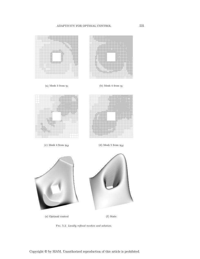
A series of meshes generated according to the information obtained from theerror estimators are shown in Figure 5.2 together with the optimal control q and thecorresponding state u.



1e-04

0.001

0.01

1000 10000 100000

globallocal η1

local ηQI

(a) Error in J

1e-06

1e-05

1e-04

0.001

0.01

1000 10000 100000

globallocal η1

local ηQI

(b) Error in I

Fig. 5.1. Discretization error for different refinement criteria.

5.2. Example 2. Our second example is motivated by a parameter identificationproblem. The minimization problem is given by

(5.5) Minimize1

2‖u− ud‖2

L2(Ω) +α

2‖q‖2

L2(Ω), u ∈ V, q ∈ Qad,

subject to

(5.6)−Δu + qu = f in Ω,

u = 0 on ∂Ω,

where Ω = ω = (0, 0.5) × (0, 1) ∪ (0, 1) × (0.5, 1), V = H10 (Ω), Q = L2(Ω), and the

admissible set Qad is given by

Qad = {q ∈ Q | q−(x) ≤ q(x) ≤ q+(x) a.e. on Ω}, with q−(x) = 0, q+(x) = 0.3 .

The desired state ud and the right-hand side f are defined as

ud(x) =1

8π2sin(2πx1) sin(2πx2), f(x) = 1,

and the regularization parameter is chosen α = 10−4. Note that for any given q ∈ Qad

the state equation (5.6) possesses a unique solution u ∈ V due to q ≥ 0.We are interested in the error in the unknown parameter, and thus we choose

I(q, u) =

∫ΩO

q(x) dx,

where ΩO = (0, 0.25) × (0.75, 1).In Table 5.2 the effectivity indices, defined as in (5.4), are listed for different types

of mesh refinement: global (uniform) refinement, random refinement, refinement basedon the error estimator η1 for the cost functional, and refinement based on the errorestimator ηQI for the quantity of interest. As in the first example we observe that theerror estimators provide quantitative information on the discretization errors.



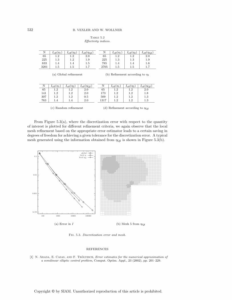
(a) Mesh 3 from η1 (b) Mesh 4 from η1

(c) Mesh 4 from ηQI (d) Mesh 5 from ηQI

(e) Optimal control (f) State

Fig. 5.2. Locally refined meshes and solution.



Table 5.2

Effectivity indices.

N Ieff(η1) Ieff(η2) Ieff(ηQI)65 1.2 1.2 2.0225 1.3 1.2 1.9833 1.4 1.4 1.53201 1.5 1.5 1.7

(a) Global refinement


(b) Refinement according to η1


(c) Random refinement


(d) Refinement according to ηQI

From Figure 5.3(a), where the discretization error with respect to the quantityof interest is plotted for different refinement criteria, we again observe that the localmesh refinement based on the appropriate error estimator leads to a certain saving indegrees of freedom for achieving a given tolerance for the discretization error. A typicalmesh generated using the information obtained from ηQI is shown in Figure 5.3(b).

(a) Error in I (b) Mesh 5 from ηQI

Fig. 5.3. Discretization error and mesh.

REFERENCES

[1] N. Arada, E. Casas, and F. Troltzsch, Error estimates for the numerical approximation ofa semilinear elliptic control problem, Comput. Optim. Appl., 23 (2002), pp. 201–229.



[2] R. Becker, Estimating the control error in the discretized PDE-constrained optimization, J.Numer. Math., 14 (2006), pp. 163–185.

[3] The Finite Element Toolkit Gascoinge; http://www.gascoigne.uni-hd.de/.[4] R. Becker, H. Kapp, and R. Rannacher, Adaptive finite element methods for optimal con-

trol of partial differential equations: Basic concept, SIAM J. Control Optim., 39 (2000),pp. 113–132.

[5] A C++ Library for Optimization with Stationary and Nonstationary PDEs; http://www.rodobo.uni-hd.de/.

[6] R. Becker and R. Rannacher, An optimal control approach to a posteriori error estimation,in Acta Numerica 2001, A. Iserles, ed., Cambridge University Press, Cambridge, UK, 2001,pp. 1–102.

[7] R. Becker and B. Vexler, A posteriori error estimation for finite element discretizations ofparameter identification problems, Numer. Math., 96 (2004), pp. 435–459.

[8] R. Becker and B. Vexler, Mesh refinement and numerical sensitivity analysis for parametercalibration of partial differential equations, J. Comput. Phys., 206 (2005), pp. 95–110.

[9] M. Bergounioux, K. Ito, and K. Kunisch, Primal-dual strategy for constrained optimalcontrol problems, SIAM J. Control Optim., 37 (1999), pp. 1176–1194.

[10] S. Brenner and R.L. Scott, The Mathematical Theory of Finite Element Methods, Springer-Verlag, Berlin, Heidelberg, New York, 1994.

[11] E. Casas, M. Mateos, and F. Troltzsch, Error estimates for the numerical approximation ofboundary semilinear elliptic control problems, Comput. Optim. Appl., 31 (2005), pp. 193–220.

[12] E. Casas and F. Troltzsch, Error estimates for linear-quadratic elliptic control problems,in Analysis and Optimization of Differential Systems (Constanta, 2002), Kluwer AcademicPublishers, Boston, MA, 2003, pp. 89–100.

[13] K. Eriksson, D. Estep, P. Hansbo, and C. Johnson, Introduction to adaptive methods fordifferential equations, in Acta Numerica 1995, A. Iserles, ed., Cambridge University Press,Cambridge, UK, 1995, pp. 105–158.

[14] K. Eriksson, D. Estep, P. Hansbo, and C. Johnson, Computational Differential Equations,Cambridge University Press, Cambridge, UK, 1996.

[15] R. S. Falk, Approximation of a class of optimal control problems with order of convergenceestimates, J. Math. Anal. Appl., 44 (1973), pp. 28–47.

[16] A. V. Fursikov, Optimal Control of Distributed Systems: Theory and Applications, Transl.Math. Monogr. 187, AMS, Providence, RI, 2000.

[17] A. Gaevskaya, R. H. W. Hoppe, Y. Iliash, and M. Kieweg, Convergence analysis of anadaptive finite element method for distributed control problems with control constraints, inControl of Coupled Partial Differential Equations, Birkhauser, Basel, 2007, pp. 47–68.

[18] T. Geveci, On the approximation of the solution of an optimal control problem governed byan elliptic equation, RAIRO Anal. Numer., 13 (1979), pp. 313–328.

[19] R. Griesse and B. Vexler, Numerical sensitivity analysis for the quantity of interest inPDE-constrained optimization, SIAM J. Sci. Comput., 29 (2007), pp. 22–48.

[20] M. Hintermuller, R. H. W. Hoppe, Y. Iliash, and M. Kieweg, An a posteriori erroranalysis of adaptive finite element methods for distributed elliptic control problems withcontrol constraints, ESAIM Control Optim. Calc. Var., to appear.

[21] M. Hintermuller, K. Ito, and K. Kunisch, The primal-dual active set strategy as a semis-mooth Newton method, SIAM J. Optim., 13 (2003), pp. 865–888.

[22] M. Hinze, A variational discretization concept in control constrained optimization: The linear-quadratic case, Comput. Optim. Appl., 30 (2005), pp. 45–61.

[23] R. H. W. Hoppe, Y. Iliash, C. Iyyunni, and N. H. Sweilam, A posteriori error estimatesfor adaptive finite element discretizations of boundary control problems, J. Numer. Math.,14 (2006), pp. 57–82.

[24] K. Kunisch and A. Rosch, Primal-dual active set strategy for a general class of constrainedoptimal control problems, SIAM J. Optim., 13 (2002), pp. 321–334.

[25] R. Li, W. Liu, H. Ma, and T. Tang, Adaptive finite element approximation for distributedelliptic optimal control problems, SIAM J. Control Optim., 41 (2002), pp. 1321–1349.

[26] J.-L. Lions, Optimal Control of Systems Governed by Partial Differential Equations,Grundlehren Math. Wiss. 170, Springer-Verlag, Berlin, 1971.

[27] W. Liu and N. Yan, A posteriori error estimates for distributed convex optimal control prob-lems, Adv. Comput. Math., 15 (2001), pp. 285–309.

[28] K. Malanowski, Convergence of approximations versus regularity of solutions for convex,control-constrained optimal-control problems, Appl. Math. Optim., 8 (1982), pp. 69–95.

[29] H. Maurer and J. Zowe, First and second-order necessary and sufficient optimality conditions



for infinite-dimensional programming problems, Math. Programming, 16 (1979), pp. 98–110.

[30] D. Meidner and B. Vexler, Adaptive space-time finite element methods for parabolic opti-mization problems, SIAM J. Control Optim., 46 (2007), pp. 116–142.

[31] C. Meyer and A. Rosch, Superconvergence properties of optimal control problems, SIAM J.Control Optim., 43 (2004), pp. 970–985.

[32] C. Meyer and A. Rosch, L∞-estimates for approximated optimal control problems, SIAM J.Control Optim., 44 (2005), pp. 1636–1649.

[33] A. Rosch, Error estimates for linear-quadratic control problems with control constraints, Op-tim. Methods Softw., 21 (2006), pp. 121–134.

[34] F. Troltzsch, Optimale Steuerung partieller Differentialgleichungen, Vieweg, Wiesbaden,Germany, 2005.

[35] R. Verfurth, A Review of A Posteriori Error Estimation and Adaptive Mesh-RefinementTechniques, Wiley/Teubner, New York, Stuttgart, 1996.

[36] B. Vexler, Adaptive Finite Elements for Parameter Identification Problems, Ph.D. thesis,Institut fur Angewandte Mathematik, Universitat Heidelberg, Heidelberg, Germany, 2004.

Documents

ADAPTIVE FINITE ELEMENTS FOR ELLIPTIC OPTIMIZATION ... · Heidelberg, Germany ([email protected]). This author’s research was sup- ported by the DFG priority