Adaptive Ensemble Models of Extreme Learning Machines for Time

Change the color of the line of the text box to ‘No line’ before printing:

Right click on the edge of the text box

Select ‘Format text box’

Select the tab ‘Colors and Lines’

Line: Color: ‘No Line’

Adaptive Ensemble Models of Extreme Learning Machines for Time Series Prediction

Mark van Heeswijk

July 2009

ii

Abstract

In time series prediction, one does often not know the properties of the underlying system

generating the time series. For example, is it a closed system that is generating the time

series or are there any external factors influencing the system? As a result of this, you

often do not know beforehand whether a time series is stationary or nonstationary, and in

the ideal case you do not want to make any assumptions about this.

Therefore, if one wants to do time series prediction on such a system it would be nice if a

model exists that is able to perform well on both nonstationary and stationary time series,

and that the model adapts itself to the environment in which it is applied.

In this thesis, we will experimentally investigate a method that hopefully has this property.

We will look at the application of adaptive ensemble models of Extreme Learning Machines

(ELMs) to the problem of one-step ahead prediction in (non)stationary time series.

In the experiments, we verify that the model works on a stationary time series, the Santa

Fe Laser Data time series. Furthermore, we test the adaptivity of the ensemble model on

a nonstationary time series, the Quebec Births time series. We show that the adaptive

ensemble model can achieve a test error comparable to or better than a state-of-the-art

method like LS-SVM, while at the same time, it remains adaptive. Additionally, the

adaptive ensemble model has low computational cost.

keywords: time series prediction, sliding window, extreme learning machine, ensemble

models, nonstationarity, adaptivity

iii

iv

Acknowledgements

This thesis has been made in Information and Computer Science Laboratory in the Adap-

tive Informatics Research Centre at the Helsinki University of Technology.

What started as a project in the Computational Cognitive Systems Group, developed into

a project in cooperation with the Time Series Prediction and Chemoinformatics Group.

Along the way, I have been very lucky to have met so many wonderful people in both

these research groups and in the lab in general. It has been great to work with all of you.

Thanks for all the nice trips, all the interesting (often late-night) discussions, and the nice

and relaxed work atmosphere in general in the lab. Combined with the good facilities at

the lab, this makes it an enjoyable and great place to work.

In particular, I would like to thank Prof. Erkki Oja for his supervision of my thesis, and

Docent Amaury Lendasse and Docent Timo Honkela for their excellent instruction, clear

guidance and mentoring, and unlimited supply of wisdom whenever needed. It has been

a pleasure and great inspiration to work with all of them. Many thanks also to Tiina

Lindh-Knuutila, who kept me focused and on-topic, whenever I could not resist asking

too many questions at once. Special thanks go out to Antti Sorjamaa, who has been a

great help in many things, ranging from LATEX support, to finding the way in the Finnish

system, to apartment hunting.

Many thanks of course go to all the people at my home university, the Eindhoven University

of Technology. First of all, I want to thank prof. dr. Peter Hilbers for his flexible

supervision, and help during my thesis. Of course, also many thanks to all the people that

helped me at one point or another during the arrangements for my thesis and my studies

in general, and helped me to get to where I am today.

Last but not least, many thanks to all my friends, and of course the wonderful people from

BEST that introduced me to Finland in the first place. It has been a great adventure so

far and I am eagerly looking forward to the years to come. Finally, love and thanks to my

parents, for always supporting me and believing in me.

Espoo July 20th 2009

Mark van Heeswijk

v

vi

Contents

Abstract iii

Acknowledgements v

Abbreviations and Notations ix

1 Introduction 1

2 Theory 3

2.1 Time Series Prediction . . . . . . . . . . . . . . . . . . . . . . . . . . . . . . 3

2.1.1 Background . . . . . . . . . . . . . . . . . . . . . . . . . . . . . . . . 3

2.1.2 Time Series . . . . . . . . . . . . . . . . . . . . . . . . . . . . . . . . 3

2.1.3 Time Series Prediction . . . . . . . . . . . . . . . . . . . . . . . . . . 4

2.2 Functional Approximation . . . . . . . . . . . . . . . . . . . . . . . . . . . . 5

2.3 Model Selection . . . . . . . . . . . . . . . . . . . . . . . . . . . . . . . . . . 7

2.3.1 Example: Influence of Model Complexity . . . . . . . . . . . . . . . 7

2.3.2 Model Selection Methods . . . . . . . . . . . . . . . . . . . . . . . . 8

2.4 Ensemble Models . . . . . . . . . . . . . . . . . . . . . . . . . . . . . . . . . 10

2.4.1 Introduction . . . . . . . . . . . . . . . . . . . . . . . . . . . . . . . 10

2.4.2 Average of Models . . . . . . . . . . . . . . . . . . . . . . . . . . . . 11

2.4.3 Related Work . . . . . . . . . . . . . . . . . . . . . . . . . . . . . . . 12

2.5 Extreme Learning Machine . . . . . . . . . . . . . . . . . . . . . . . . . . . 12

3 Adaptive Ensemble Models 15

3.1 Adaptive Ensemble Model . . . . . . . . . . . . . . . . . . . . . . . . . . . . 15

3.2 Adaptive Ensemble Model of ELMs . . . . . . . . . . . . . . . . . . . . . . . 16

3.2.1 Initialization of the Ensemble Model using PRESS Residuals . . . . 16

3.2.2 Adaptation of the Ensemble . . . . . . . . . . . . . . . . . . . . . . . 17

3.2.3 Adaptation of the Models . . . . . . . . . . . . . . . . . . . . . . . . 18

4 Experiments 21

vii

4.1 Time Series . . . . . . . . . . . . . . . . . . . . . . . . . . . . . . . . . . . . 22

4.1.1 Motivation for the Choice of Time Series . . . . . . . . . . . . . . . 22

4.1.2 Stationary Time Series - Santa Fe Laser Data . . . . . . . . . . . . . 22

4.1.3 Nonstationary Time Series - Quebec Births . . . . . . . . . . . . . . 22

4.2 Experiments . . . . . . . . . . . . . . . . . . . . . . . . . . . . . . . . . . . . 25

4.2.1 Experiment 1: Adaptive Ensembles of ELMs . . . . . . . . . . . . . 25

4.2.2 Experiment 2a: Sliding Window Retraining . . . . . . . . . . . . . . 29

4.2.3 Experiment 2b: Growing Window Retraining . . . . . . . . . . . . . 31

4.2.4 Experiment 3: Initialization based on Leave-One-Out Output . . . . 33

4.2.5 Experiment 4: Running Times and Least Squares Support Vector

Machine . . . . . . . . . . . . . . . . . . . . . . . . . . . . . . . . . . 33

5 Discussion 39

5.1 Effect of Number of Models . . . . . . . . . . . . . . . . . . . . . . . . . . . 39

5.2 Effect of Learning Rate . . . . . . . . . . . . . . . . . . . . . . . . . . . . . 39

5.3 Effect of the Leave-one-out Weight Initialization . . . . . . . . . . . . . . . 40

5.4 LS-SVM and Performance Considerations . . . . . . . . . . . . . . . . . . . 41

5.4.1 Comparing models . . . . . . . . . . . . . . . . . . . . . . . . . . . . 42

5.4.2 Comparison on Laser Time Series . . . . . . . . . . . . . . . . . . . . 42

5.4.3 Comparison on Quebec Time Series . . . . . . . . . . . . . . . . . . 43

6 Future Work 45

6.1 Explore Links with Other Fields . . . . . . . . . . . . . . . . . . . . . . . . 45

6.2 Improving on Input Selection . . . . . . . . . . . . . . . . . . . . . . . . . . 45

6.3 Improving Individual Models . . . . . . . . . . . . . . . . . . . . . . . . . . 45

6.4 Improving Ensemble Model . . . . . . . . . . . . . . . . . . . . . . . . . . . 46

6.5 Other Degrees of Adaptivity . . . . . . . . . . . . . . . . . . . . . . . . . . . 46

6.6 Parallel implementation . . . . . . . . . . . . . . . . . . . . . . . . . . . . . 47

6.7 GPU Computing . . . . . . . . . . . . . . . . . . . . . . . . . . . . . . . . . 47

7 Conclusions 49

8 Bibliography 51

8.1 References . . . . . . . . . . . . . . . . . . . . . . . . . . . . . . . . . . . . . 51

A Santa Fe Laser Data Errors 55

B Quebec Birth Data Errors 57

viii

Abbreviations and Notations

ELM Extreme Learning Machine

i.i.d. independent and identically distributed

MSE Mean Square Error

LS-SVM Least Squares Support Vector Machine

d the dimension of the input samples

M the number of samples

m the number of models

N the number of hidden neurons

x(t) input value x, at time t

y(t) true value y, at time t

(xi, yi) training sample consisting of input xi and output yi

xi 1 × d vector of input values

yi output value

X M × d matrix of inputs

Y M × 1 matrix of outputs

yi(t) approximated output y by model i, at time t

yens(t) approximated output y by ensemble, at time t

ǫi(t) error of model i, at time t

E[x] expectation of x

wi the input weights to the ith neuron in the hidden layer

bi the biases of the ith neuron in the hidden layer

H hidden layer output matrix

H† Pseudo-inverse of matrix H (i.e. (HTH)−1HT )

βi the output weights

ix

x

List of Figures

2.1 A schematic overview of a system . . . . . . . . . . . . . . . . . . . . . . . . 3

2.2 A schematic overview of the relation between a model and the system it is

trying to model . . . . . . . . . . . . . . . . . . . . . . . . . . . . . . . . . . 4

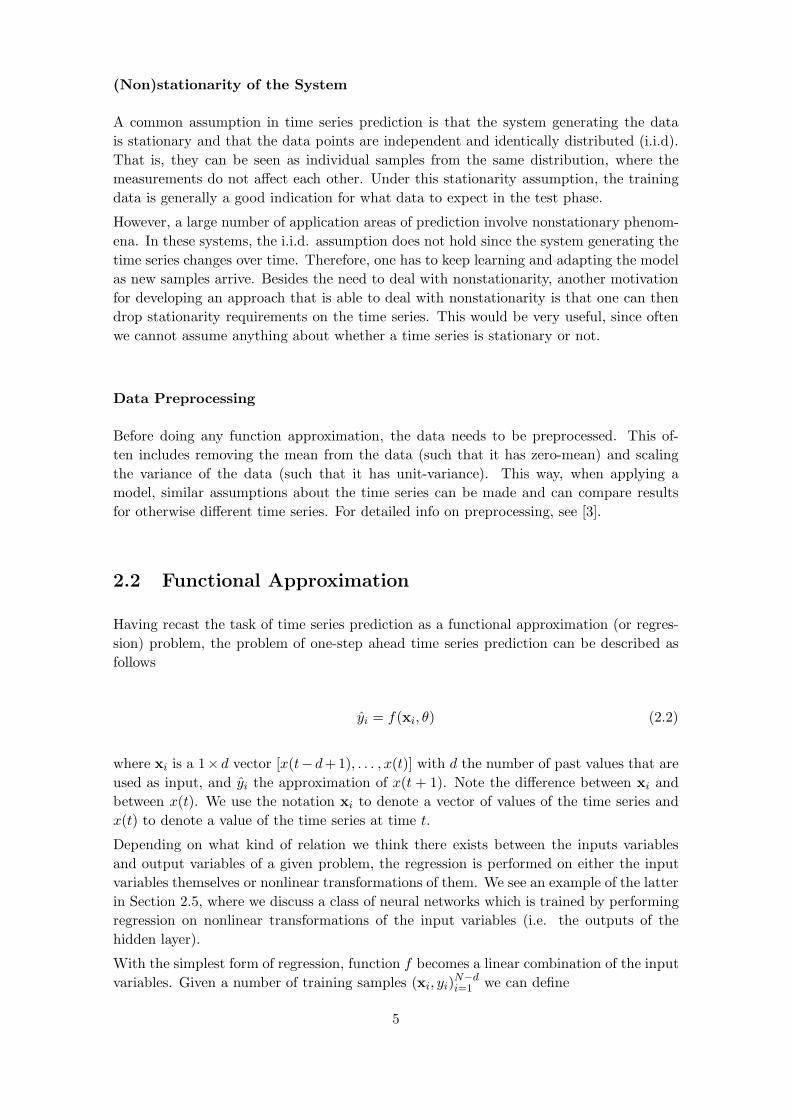
2.3 Output of various models (red line), trained on a number of points (blue

dots) of the underlying function (green line) . . . . . . . . . . . . . . . . . . 8

2.4 The effect of model the number of hidden neurons on test error . . . . . . . 9

2.5 A schematic overview of how models can be combined in an ensemble . . . 11

2.6 A schematic overview of an ELM . . . . . . . . . . . . . . . . . . . . . . . . 13

3.1 A schematic overview of how ELMs can be combined in an ensemble . . . . 16

3.2 Plots showing part of the ensemble weights wi adapting over time during

sequential prediction on (a) Laser time series and (b) Quebec Births time

series (learning rate=0.1, number of models=10) . . . . . . . . . . . . . . . 18

4.1 The Santa Fe Laser Data time series (first 1000 values) . . . . . . . . . . . . 23

4.2 The Santa Fe Laser Data time series (complete) . . . . . . . . . . . . . . . . 23

4.3 The Quebec Births time series (first 1000 values) . . . . . . . . . . . . . . . 24

4.4 The Quebec Births time series (complete) . . . . . . . . . . . . . . . . . . . 24

4.5 The result of a single run: a measurement of the mean square test error

over all parameter combinations . . . . . . . . . . . . . . . . . . . . . . . . . 26

4.6 MSEtest of ensemble on Laser time series as a function of (a) the number

of models and (b) the learning rate, with individual runs (gray lines), the

mean of all runs (black line), and the standard deviation on all runs (error

bars). . . . . . . . . . . . . . . . . . . . . . . . . . . . . . . . . . . . . . . . 27

4.7 Distribution of MSEtest of 100 individual models on Laser time series. . . . 27

4.8 MSEtest of ensemble on Quebec time series as a function of (a) the number

of models and (b) the learning rate, with individual runs (gray lines), the

mean of all runs (black line), and the standard deviation on all runs (error

bars). . . . . . . . . . . . . . . . . . . . . . . . . . . . . . . . . . . . . . . . 28

4.9 Distribution of MSEtest of 100 individual models on Quebec time series. . . 28

4.10 MSEtest of ensemble (retrained on sliding window) on Laser time series as

a function of (a) the number of models and (b) the learning rate, with

individual runs (gray lines), the mean of all runs (black line), and the

standard deviation on all runs (error bars). . . . . . . . . . . . . . . . . . . 29

xi


4.12 MSEtest of ensemble (retrained on sliding window) on Quebec time series

as a function of (a) the number of models and (b) the learning rate, with




4.14 MSEtest of ensemble (retrained on sliding window) on Laser time series as

a function of (a) the number of models and (b) the learning rate, with




4.16 MSEtest of ensemble (retrained on sliding window) on Quebec time series

as a function of (a) the number of models and (b) the learning rate, with




4.18 Comparison of MSEtest on Laser time series for uniform weight initializa-

tion (solid lines) and on leave-one-out initialization (dotted lines) for: no

retraining (blue lines), sliding window retraining (red lines) and growing

window retraining (green lines). . . . . . . . . . . . . . . . . . . . . . . . . . 34

4.19 Comparison of MSEtest on Quebec time series for uniform weight initializa-

tion (solid lines) and on leave-one-out initialization (dotted lines) for: no



4.20 Running time of the ensemble on Laser series for varying numbers of models

for uniform initialization (solid lines), LOO initialization (dotted lines), no



4.21 Running time of the ensemble on Quebec series for varying numbers of

models for uniform initialization (solid lines), LOO initialization (dotted

lines), no retraining (blue lines), sliding window retraining (red lines) and

growing window retraining (green lines). . . . . . . . . . . . . . . . . . . . . 37

5.1 MSEtest as a function of learning rate for (a) Laser time series and (b)

Quebec time series for 10 models (dashed line) and 100 models (solid line). 40

xii

List of Tables

4.1 Parameters for Experiment 1 . . . . . . . . . . . . . . . . . . . . . . . . . . 25

4.2 Average time (s) a single model adds to running time of ensemble on Laser 36

4.3 Average time (s) a single model adds to running time of ensemble on Quebec 37

4.4 Parameters used for LS-SVM . . . . . . . . . . . . . . . . . . . . . . . . . . 38

4.5 LS-SVM Results . . . . . . . . . . . . . . . . . . . . . . . . . . . . . . . . . 38

A.1 Average prediction error on Santa Fe Laser Data (learning rate=0.1) . . . . 55

A.2 Average prediction error on Santa Fe Laser Data (learning rate=0.1) . . . . 55

A.3 Average prediction error on Santa Fe Laser Data (#models=100) . . . . . . 56

B.1 Average prediction error on Quebec Births (learning rate=0.1) . . . . . . . 57

B.2 Average prediction error on Quebec Births (learning rate=0.1) . . . . . . . 57

B.3 Average prediction error on Quebec Births (#models=100) . . . . . . . . . 58

xiii

xiv

Chapter 1

Introduction

In many fields one encounters data or measurements which vary in time. Given this data,

one wants to gain insight in the system generating the data and predict how the system

will behave in the future given the data so far. For example, in finance, experts predict

stock exchange courses or stock market indices, and producers of electricity predict the

load of the following day. In all these fields, the common question is how one can analyze

and use the past to predict the future.

In time series prediction, one of the challenges is that one does often not know the prop-

erties of the underlying system generating the time series. For example, we often do not

have complete knowledge about whether the system is a closed system that is generating

the time series and whether or not there are any external factors influencing the system.

As a result of this, we often do not know beforehand whether a time series is stationary

or nonstationary.

Therefore, in the ideal case we do not want to make any assumptions about the stationarity

of the system and it would be nice if the model we use to predict future values of the time

series is able to perform well on both nonstationary and stationary time series and that

the model adapts itself to the environment in which it is applied.

In this thesis, we look at the problem of one-step ahead prediction on both stationary and

nonstationary time series. What this means is that at any time, we would like to predict

the next value in the time series as accurate as possible, using the past values of the time

series. The model we will use for this task is an adaptive ensemble model of a type of

feedforward neural network called Extreme Learning Machines.

With this model, we use various strategies in order to make it adaptive to changes in the

environment it is operating in. First of all, we use a combination of multiple models, each

of which is specialized on part of the state space. We combine these models in an adaptive

way in order to optimize prediction accuracy. Secondly, we look at different strategies to

retraining the models repeatedly on a finite window of past values.

We experimentally investigate the model on both stationary and nonstationary time series,

and analyze the model and the influence of its parameters on both prediction accuracy

and performance.

In the experiments, we verify that the model works on a stationary time series, the Santa

Fe Laser Data time series and achieves good prediction accuracy and performance. We

also test the adaptivity of the ensemble model on a nonstationary time series, the Quebec

Births time series. We show that the adaptive ensemble model can achieve a test error

1

comparable or better to a state-of-the-art method like the Least Squares Support Vector

Machine (LS-SVM), while at the same time, remaining adaptive. Additionally, we show

that it is able to do so at low computational cost.

The organization of the rest of this thesis is as follows. First, in Chapter 2 we discuss the

theory related to the topic of this thesis. In particular time series prediction and its goals,

regression, model selection, ensemble models, and Extreme Learning Machines.

Once an overview of the theory has been given, in Chapter 3 we discuss how the various

parts come together in the ensemble models that are the focus of this thesis. We will

introduce multiple degrees of adaptivity, show how the proposed model can be trained at

little computational cost and in what context it is applied.

In Chapter 4 and 5, we discuss and analyze the experiments which we performed to

investigate the performance of the ensemble model in one-step ahead prediction on the two

different time series. We verify that the model works on a stationary time series, the Santa

Fe Laser Data time series and investigate the adaptivity of the model on the nonstationary

time series, the Quebec Births Data. We will look at the quality of predictions made by

the ensemble model and the LS-SVM, as well as the computational requirements of the

different methods.

We conclude the by giving an overview of promising future research directions and sum-

marize the results of the thesis.

2

Chapter 2

Theory

2.1 Time Series Prediction

2.1.1 Background

In many fields one encounters data or measurements which vary in time. Given this data,

one often want to gain some insight in the underlying system generating the data or predict

future data points given the data so far. This is what time series prediction deals with.

Time series prediction is a challenge in many fields. For example, in finance, experts

predict stock exchange courses or stock market indices; data processing specialists predict

the flow of information on their networks; producers of electricity predict the load of the

following day [1, 2], climatologists want to predict the change in temperature as a result

of CO2 emmissions. In all these fields, the common question is how one can analyze and

use the past to predict the future.

2.1.2 Time Series

A common assumption in the field of time series prediction is that the underlying process

generating the data is not changing over time (i.e. is stationary), and that the data

points generated by the process are independent and identically distributed. A schematic

overview of a system can be found in Figure 2.1.

System

disturbances

u xu x

Figure 2.1: A schematic overview of a system

Here the inputs of the system are denoted by u, the outputs of the system are denoted by

xu. We often do not know xu but only observe a noisy version of the outputs, namely x.

For example, if we would describe the electricity grid and the load on it this way, then all

3

the factors that are influencing the electricity grid (like time of day, season, temperature)

are denoted by u, the load on the electricity grid as xu, and the measurement of it as x.

A series of these measurements makes up a time series, which can be formally defined as

{x(t)}Nt=1, x(t) ∈ R, (2.1)

where t denotes the time. The time step between two consecutive values in a time series

is equal across the entire time series and can range from microseconds to years. In case

both u(t) and x(t) are both part of the time series, then we speak of a time series with

external inputs. In this thesis however, the focus is on time series without external inputs.

2.1.3 Time Series Prediction

Model and System

Now, given past values of a time series, the goal is to predict future values of the time

series. A common way to do this is by considering the system generating the data as

an autoregressive process, and try to build a model that approximates the input-output

relation of that process as good as possible. That is, to see the values of the time series

as a function of previous values and to approximate this function as closely as possible.

The relation between model and process is depicted in Figure 2.2.

System

Model f(x, θ)

disturbances

x yu y

−

y

ǫ

Figure 2.2: A schematic overview of the relation between a model and the system it is

trying to model

Contrary to Figure 2.1, where the input variables were external variables, input x now

consists of previous values of the time series. The goal is to find a model f(x, θ) with

inputs x and n-dimensional parameter vector θ that approximates y as good as possible.

This can be seen as finding the point in the n-dimensional parameter space that minimizes

some cost criterion.

Besides parameter optimization of the model, on can also do structural optimization of

the model. Here, one optimizes for example what kind of function f is best to use, and the

optimal number of parameters for that function f . It is important that we structurally

optimize the model which we intend to use for the time series prediction.

4

(Non)stationarity of the System

A common assumption in time series prediction is that the system generating the data

is stationary and that the data points are independent and identically distributed (i.i.d).

That is, they can be seen as individual samples from the same distribution, where the

measurements do not affect each other. Under this stationarity assumption, the training

data is generally a good indication for what data to expect in the test phase.

However, a large number of application areas of prediction involve nonstationary phenom-

ena. In these systems, the i.i.d. assumption does not hold since the system generating the

time series changes over time. Therefore, one has to keep learning and adapting the model

as new samples arrive. Besides the need to deal with nonstationarity, another motivation

for developing an approach that is able to deal with nonstationarity is that one can then

drop stationarity requirements on the time series. This would be very useful, since often

we cannot assume anything about whether a time series is stationary or not.

Data Preprocessing

Before doing any function approximation, the data needs to be preprocessed. This of-

ten includes removing the mean from the data (such that it has zero-mean) and scaling

the variance of the data (such that it has unit-variance). This way, when applying a

model, similar assumptions about the time series can be made and can compare results

for otherwise different time series. For detailed info on preprocessing, see [3].

2.2 Functional Approximation

Having recast the task of time series prediction as a functional approximation (or regres-

sion) problem, the problem of one-step ahead time series prediction can be described as

follows

yi = f(xi, θ) (2.2)

where xi is a 1× d vector [x(t− d+1), . . . , x(t)] with d the number of past values that are

used as input, and yi the approximation of x(t + 1). Note the difference between xi and

between x(t). We use the notation xi to denote a vector of values of the time series and

x(t) to denote a value of the time series at time t.

Depending on what kind of relation we think there exists between the inputs variables

and output variables of a given problem, the regression is performed on either the input

variables themselves or nonlinear transformations of them. We see an example of the latter

in Section 2.5, where we discuss a class of neural networks which is trained by performing

regression on nonlinear transformations of the input variables (i.e. the outputs of the

hidden layer).

With the simplest form of regression, function f becomes a linear combination of the input

variables. Given a number of training samples (xi, yi)N−di=1 we can define

5

X =

x(1) x(2) . . . x(d)

x(2) x(3) . . . x(d + 1)...

.... . .

...

x(N − d) x(N − d + 1) . . . x(N − 1)

,

Y =

x(d + 1)

x(d + 2)...

x(N)

(2.3)

where d is the number of inputs and N the number of training samples. The matrix X is

also know as the regressor matrix and each row contains an input, while the corresponding

row in Y contains the corresponding target to approximate.

If we denote the weight vector [β1, . . . , βd]T by β, then the optimal weight vector can be

computed by solving the system

Xβ = Y. (2.4)

This weight vector is optimal in the sense that it gives the least mean square error (MSE)

approximation of the training targets, given input X.

The optimal weight vector can be computed as follows [4]:

Xβ = Y

XTXβ = XTY

(XTX)−1(XTX)β = (XTX)−1XTY

β = X†Y

where X† is known as the pseudo-inverse or Moore-Penrose inverse [5].

Furthermore, since the approximation of the output for given X and β is defined as

Y = Xβ we get

Y = Xβ

= X(XTX)−1XTY

= HAT ·Y

where HAT is defined as X(XTX)−1XT . The HAT-matrix is the matrix that transforms

the output Y into the approximated output Y . We see the HAT-matrix later again when

we discuss PRESS statistics in Section 3.2.1.

Instead of doing regression on the input, one can also consider linear combinations of

nonlinear functions of the input variables (called basis functions). This approach is a lot

more powerful and can, given enough basis functions, approximate any given function

under the condition that these basis functions are infinitely differentiable. In other words,

they are universal approximators [6].

6

2.3 Model Selection

As mentioned earlier, one can optimize the parameters of a model as well as the structure

of a model. In optimizing the structure of a model, one generates a collection of models to

compare, and then evaluates them according to some criteria. The models being compared

can be different in a lot of ways. Some examples of where models can structurally differ

are

• the number of neurons in the hidden layer of a neural network,

• the number of layers in the neural network,

• the learning algorithm being used to train a neural network,

• the size of the regressor (i.e. the number of variables being taken as input),

• which variables are used to build the regressor (i.e. we could build a regressor that

contains only the values x(t − 5), x(t − 10), x(t − 11) as input at time t),

• which basis functions are being used in the hidden layer of the neural network,

• any other parameters defining the structure of the model that are not being trained

2.3.1 Example: Influence of Model Complexity

In selecting the right model, the model complexity is an important factor. If the model

is too complex, it will perfectly fit the training data, but will have bad generalization on

data other than the training data. On the other hand, if the model is too simple, it will

not be able to approximate the training data at all. These cases are known as overfitting

and underfitting.

Figure 2.3a shows training data and the output of a too simple model. It is obvious that

the model is not able to learn the functional mapping between inputs and outputs.

Figure 2.3b shows the same training data, but this time with the output of a too complex

model. While it perfectly approximates the points it was trained on, it can be seen that

it has poor generalization performance and does not approximate the underlying function

of the data very well.

Figure 2.3c shows a model that shows good approximation performance on the data it was

trained on, and at the same time approximates the underlying function of the data well.

From these examples, it becomes clear that there is a trade-off between accuracy of the

model on the training set, and the generalization performance of the model on the test

set.

In Figure 2.4 the effect of the number of hidden neurons in a feedforward neural network

(Extreme Learning Machine) on the test error can be seen. Since there is some variability

in the test error because of the random nature of the model, we repeat the experiment

50 times (gray lines) and show the mean (black line) and the standard deviation for all

measurements.

From this example, it seems obvious what is the optimal model complexity. However,

keep in mind that in this example we are using the test set in order to determine the

optimal model complexity. Normally, at the time where we need to select the optimal

7

−1 −0.5 0 0.5 1−3

−2

−1

0

1

2

X

Y

(a) underfitting

−1 −0.5 0 0.5 1−3

−2

−1

0

1

2

X

Y

(b) overfitting

−1 −0.5 0 0.5 1−3

−2

−1

0

1

2

X

Y

(c) good fit

−1 −0.5 0 0.5 1−3

−2

−1

0

1

2

X

Y

(d) combined

Figure 2.3: Output of various models (red line), trained on a number of points (blue dots)

of the underlying function (green line)

model complexity, we do not have the test data yet. Or, if we have, then using the test

data in determining the model complexity can be considered as cheating.

Luckily, there exist various ways to estimate what would be the test error, otherwise

known as the generalization error, by just using the training set. Here, we discuss three of

them: validation, k-fold crossvalidation and leave-one-out crossvalidation. See [4] and [7]

for detailed information on these methods.

2.3.2 Model Selection Methods

As we have seen in the example above, a good model performs well on the training set,

and the input-output mapping that the model learned from the training set transfers well

to the test set. In other words, the model approximates the underlying function of the

data well and has good generalization.

How well a model generalizes can be measured in the form of the generalization error

which is defined as

Egen(θ) = limM→∞

∑Mi=1(f(xi, θ) − yi)

2

M(2.5)

where M is the number of samples, xi is the d-dimensional input, θ contains the model

8

0 100 200 300 400 500 600 700 8000

50

100

150

number of hidden neurons

mea

n sq

uare

test

err

or

Figure 2.4: The effect of model the number of hidden neurons on test error

parameters, and yi is the output corresponding to input vector xi.

Of course, in reality we do not have an infinite number of samples. What we do have is

a training set and a test set, consisting of samples that the model will be trained on and

samples that the model will be tested on, respectively. Therefore, the training set is to be

used to estimate the generalization performance, and thus the quality, of a given model.

We will now discuss three different methods that are often used in model selection and

the estimation of the generalization error of a model.

Validation

In using validation, one sets aside part of the training set in order to evaluate the general-

ization performance of the trained model. If we denote the indexes of the samples in the

validation set by val and the indexes of the samples in the full training set by train, then

the estimation of the generalization error is defined as

EVALgen (θ∗) =

∑

i∈val(f(xi, θ∗trainrval) − yi)

2

|val|(2.6)

where θ∗trainrval denotes the model parameters trained on all samples that are in the

training set, but not in the validation set. Note that after the validation procedure and

selecting the model, the model is trained on the full training set.

The problem with this validation procedure is that is not that reliable, since we are

only holding out a small part of the data for validation, and we have no idea of how

representative this sample is for the test set. It would be better if we could use the

training set more effectively. This is exactly what k-fold crossvalidation does.

9

k-Fold Crossvalidation

In k-fold crossvalidation, we do exactly the same thing as in validation, but now we divide

the training set into k parts, each of which is used as validation set once, while the rest of

the samples are used for training. The final estimation of the generalization error is the

mean of the generalization errors obtained in each fold

EkCVgen (θ∗) =

∑ks=1

[∑

i∈vals(f(xi, θ

∗trainrvals

) − yi)2]

M(2.7)

where θ∗trainrvalsdenotes the model parameters trained on all samples that are in the

training set, but not in validation set vals.

In practice, it is common to use k = 10. k-fold crossvalidation gives a better estima-

tion of the generalization error, but since we are doing the validation k times it is more

computationally intensive than validation.

Leave-one-out Crossvalidation

Leave-one-out (LOO) crossvalidation is basically a special case of k-fold crossvalidation,

namely the case where k = n. The models are trained on M training sets, in each of which

exactly one of the samples has been left out. The left-out sample is used for testing, and

fhe final estimation of the generalization error is the mean of the M obtained errors

ELOOgen (θ∗) =

∑Mi=1(f(xi, θ

∗−i) − yi)

2

M(2.8)

where θ∗−i denotes the model parameters trained on all samples that are in the training

set except on sample i.

Due to the fact that we make maximum use of the training set, the LOO crossvalidation

gives the most reliable estimate of the generalization error. While the amount of compu-

tation for LOO crossvalidation might seem excessive, in many cases one can apply some

mathematical tricks to prevent a lot of computation. Therefore, it does not need as much

computation as one might think. In Section 3.2.3 we will see an example of this.

2.4 Ensemble Models

2.4.1 Introduction

To explain ensemble models, it is helpful to first look to an example from real life. You

might know of these contests at events where you need to guess the number of marbles

in a glass vase. The person who makes the best guess wins the price. It turns out that

while each individual guess is likely to be pretty far of, the average of all guesses is a good

estimate of real number of marbles in the vase. This phenomenon is often referred to as

’wisdom of the crowds’.

A similar strategy is employed in the building of ensemble models. An ensemble model

combines multiple individual models, with the goal of reducing the expected error of

the model. Commonly, this is done by taking the average or a weighted average of the

individual models (see Figure 2.5), but other combination schemes are also possible [8].

10

For example, one could take the best n models and take a linear combination of those. A

good overview of ensemble methods is given by [4]. For an article focusing specifically on

ensembles of neural networks, see [9].

model1x

· · ·x

modelmx

Σ yens(t)

models ensemble

w1y1(t)

wmym(t)

Figure 2.5: A schematic overview of how models can be combined in an ensemble

2.4.2 Average of Models

Ensemble methods rely on having multiple good models with sufficiently uncorrelated

error. As described above, a common way to build an ensemble model is to take the

average of the individual models, in which case the output of the ensemble model becomes:

yens(t) =1

m

m∑

i=1

yi(t)), (2.9)

where yens(t) is the output of the ensemble model, yi(t) are the outputs of the individual

models and m is the number of models.

Following [4], it can be shown that the variance of the ensemble model is lower than the

average variance of all the individual models:

Let y(t) denote the true output that we are trying to predict and yi(t) the estimation for

this value of model i. Then, we can write the output yi(t) of model i as the true value

y(t) plus some error term ǫi(t):

yi(t) = y(t) + ǫi(t). (2.10)

Then the expected square error of a model becomes

E[{

yi(t) − y(t)}2

] = E[ǫi(t)2]. (2.11)

The average error made by a number of models is given by

Eavg =1

m

m∑

i=1

E[ǫi(t)2]. (2.12)

Similarly, the expected error of the ensemble as defined in Equation 2.9 is given by

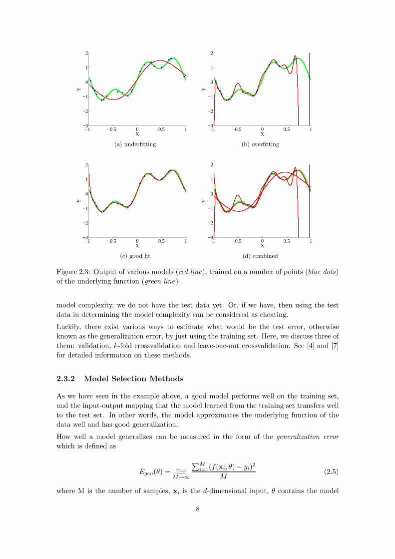
11

Eens = E

[{ 1

m

m∑

i=1

yi(t) − y(t)}2]

= E

[{ 1

m

m∑

i=1

ǫi(t)}2]

. (2.13)

Assuming the errors ǫi(t) are uncorrelated (i.e. E[ǫi(t)ǫj(t)] = 0) and have zero mean

(E[ǫi(t)] = 0), we get

Eens =1

mEavg . (2.14)

Note that these equations assume completely uncorrelated errors between the models,

while in practice errors tend to be highly correlated. Therefore, errors are often not

reduced as much as suggested by these equations, but can be improved by using ensemble

models. It can be shown that Eens < Eavg always holds. Note that this only tells us that

the test error of the ensemble is smaller than the average test error of the models, and that

it is not necessarily better than the best model in the ensemble. Therefore, the models

used in the ensemble should be sufficiently accurate.

2.4.3 Related Work

Ensemble models have been applied in various forms (and under various names) to time

series prediction, regression and classification. A non-exhaustive list of literature that dis-

cusses the combination of different models into a single model includes bagging [10], boost-

ing [11], committees [4], mixture of experts [12], multi-agent systems for prediction [13],

classifier ensembles [8], among others. Out of these examples, the work presented in this

thesis is most closely related to [13], which describes a multi-agent system prediction of

financial time series and recasts prediction as a classification problem. Other related work

includes [8], which deals with classification under concept drift (nonstationarity of classes).

The difference is that both papers deal with classification under nonstationarity, while we

deal with regression under nonstationarity.

2.5 Extreme Learning Machine

The Extreme Learning Machine (ELM) model has been proposed by Guang-Bin Huang

et al. in [14]. It is a type of Single-Layer Feedforward Neural Network (SLFN) and it

can be used for function approximation (regression) and classification. Most traditional

algorithms for training a SLFN use some learning rule that adapts all the weights based

on the showing of a single training example or a batch of training examples [3].

Extreme Learning Machines on the other hand, rely on certain properties of the network.

Namely, if the weights and biases in the input layer are randomly initialized, and the

transfer functions in the hidden layer are infinitely differentiable, then the optimal output

weights for a given training set can be determined analytically. The obtained output

weights minimize the square training error.

Since the network is trained in very few steps it is very fast to train, and it is therefore

an attractive candidate model for use in a function approximation problem. A schematic

overview of the structure of the ELM can be seen in Figure 2.6.

12

input xi1

input xi2

input xi3

input xi4

output yi

Hidden

layer

Input

layer

Output

layer

Figure 2.6: A schematic overview of an ELM

Now, we will review the main concepts of ELM as presented in [14] in more detail.

Consider a set of M distinct samples (xi, yi) with xi ∈ Rd and yi ∈ R; then, a SLFN with

N hidden neurons is modeled as the following sum

N∑

i=1

βif(wixj + bi), j ∈ [1,M ], (2.15)

where f is the activation function, wi are the input weights to the ith neuron in the hidden

layer, bi the biases and βi are the output weights.

In the case where the SLFN would perfectly approximate the data (meaning the error

between the output yi and the actual value yi is zero), the relation is

N∑

i=1

βif(wixj + bi) = yj, j ∈ [1,M ], (2.16)

which can be written compactly as

Hβ = Y, (2.17)

where H is the hidden layer output matrix defined as

H =

f(w1x1 + b1) · · · f(wNx1 + bN )...

. . ....

f(w1xM + b1) · · · f(wNxM + bN )

, (2.18)

and β = (β1 . . . βN )T and Y = (y1 . . . yM )T .

Given the randomly initialized first layer of the ELM and the training inputs xi ∈ Rd, the

hidden layer output matrix H can be computed. Now, given H and the target outputs

yi ∈ R (i.e. Y), the output weights β can be solved from the linear system defined

by Equation 2.17. This solution is given by β = H†Y, where H† is the Moore-Penrose

generalized inverse of the matrix H [5]. This solution for β is the unique least-squares

solution to the equation Hβ = Y.

13

Overall, the ELM algorithm now can be summarized as:

Algorithm 1 ELM

Given a training set (xi, yi),xi ∈ Rd, yi ∈ R, an activation function f : R 7→ R and N the

number of hidden nodes,

1: - Randomly assign input weights wi and biases bi, i ∈ [1, N ];

2: - Calculate the hidden layer output matrix H;

3: - Calculate output weights matrix β = H†Y.

Theoretical proofs and more details on the ELM algorithm can be found in the original

paper [14] and in [15].

14

Chapter 3

Adaptive Ensemble Models

3.1 Adaptive Ensemble Model

When creating a model to solve a certain regression or classification problem, it is unknown

in advance what the optimal model complexity and structure is. Therefore, as discussed

in Section 2.3.2 we should optimize the model structure by means of of a model selection

method like validation, crossvalidation or leave-one-out validation. Doing this, can be quite

costly however, and in case we are dealing with a nonstationary process generating the

data, it is not guaranteed that the model which we select based on a set of training samples

will be the best model 100 or a 1000 time steps later. In the case of a nonstationary process

the i.i.d. assumption does not hold, and the information gathered from past samples can

become inaccurate. Therefore, it is required to keep learning and keep adapting the model

once new samples become available.

Possible ways of doing this include:

• using a combination of different models (each of which is specialized on a part of the

state space), and do online model selection

• retraining the model repeatedly on a finite window into the past, such that it ’follows’

the nonstationarity

In this thesis, we investigate both strategies in one-step ahead prediction on (non)stationary

time series, in which we predict the next value of the time series, given all its past values.

On the one hand, we combine a number of different models in a single ensemble model

and adapt the weights with which these models contribute to the ensemble. The idea

behind this is that as the time series changes, a different model will be more optimal to

use in prediction. By monitoring the errors that the individual models in the ensemble

make, we can give higher weight to the models that have good prediction performance for

the current part of the time series, and lower weight the models that have bad prediction

performance for the current part of the time series.

On the other hand, we retrain the individual models on a limited number of past values

(sliding window) or on all known values (growing window). This way, the models will

be adapting to the changing input-output mapping that is a result of the nonstationary

character of the system generating the time series.

Now we will discuss in more detail how we combine different ELMs in an a single ensemble

15

model, how we adapt the ensemble weights, and how we adapt the models themselves.

3.2 Adaptive Ensemble Model of ELMs

The ensemble model consists of a number of randomly initialized ELMs, which each have

their own parameters (as discussed in Section 2.5). So each model can have different

regressor variables and size, different number of hidden neurons, and different biases and

input layer weights.

The model ELMi has an associated weight wi which determines its contribution to the

prediction of the ensemble. Each ELM is individually trained on the training data and the

outputs of the ELMs contribute to the output yens of the ensemble as follows: yens(t) =∑

i wiyi(t). See Figure 3.1 for a schematic overview of this.

ELM1x

· · ·x

ELMmx

Σ yens(t)

models ensemble

w1y1(t)

wmym(t)

Figure 3.1: A schematic overview of how ELMs can be combined in an ensemble

For initialization of the ensemble model, each of the individual models is trained on a given

training set, and initially each model contributes with the same weight to the output of

the ensemble. We will refer to this as uniform weight initialization.

3.2.1 Initialization of the Ensemble Model using PRESS Residuals

As an alternative to uniform weight initialization, we can try to improve the initial weights

by basing them on the leave-one-out output of the models on the training set. We will

refer to this as leave-one-out weight initialization.

The leave-one-out output can be computed from the true output and the leave-one-out

error, which we already saw in Section 2.3.2. The definition of the leave-one-out error is

ǫi,−i = yi − xib−i = yi − yi,−i. (3.1)

where ǫi,−i is the leave-one-out error when we leave out sample i, yi is the target output

specified by sample i from the training set, and b−i are the obtained weights when we

train the model on the training set with sample i left out.

The leave-one-out error ǫi,−i is also known as a PRESS residual, since it is used in the

PRESS (Prediction Sum of Squares) statistic [16]. The PRESS statistic is defined as

16

PRESS =

M∑

i=1

(yi − yi,−i)2 =

M∑

i=1

(ǫi,−i)2. (3.2)

and is closely related to the estimation of the generalization error of a model by leave-one-

out crossvalidation (see Section 2.3.2).

Although it might seem that there is a lot of computation involved in the computation of

ǫi,−i (i.e. we need to train M models), it can be computed quite efficiently. Namely, it

turns out that we can compute the PRESS residuals from the ordinary residuals (i.e. the

errors of the trained model on the training set) as follows

ǫi,−i =ǫi

1 − xi(XTX)−1xT

i

=yi − yi

1 − xi(XTX)−1xT

i

=yi − xib

1 − xi(XTX)−1xT

i

=yi − xib

1 − hii

where hii is the diagonal of the HAT matrix X(XTX)−1XT , which we already encountered

in Section 2.2. Therefore, we only need to train the model once on the entire training set

in order to obtain b, and compute the HAT matrix once. Once we have computed those,

all the PRESS residuals can easily be derived using the above equation. Obviously, this

involves a lot less computation than training the model for all M possible training sets.

Using the obtained PRESS residuals, we can compute the leave-one-out outputs through

Equation 3.1. Given the leave-one-out outputs for all m models, we perform linear regres-

sion1 on these m vectors in order to fit them to the target outputs of the training set and

to obtain the initial ensemble weights. Using this procedure, models that have bad gen-

eralization performance get relatively low weight, while models with good generalization

performance get higher weights.

3.2.2 Adaptation of the Ensemble

Once initial training of the models on the training set is done, repeated one-step ahead

prediction on the ’test’ set starts. After each time step, the previous predictions yi(t − 1)

are compared with the real value y(t− 1). If the square error ǫi(t− 1)2 of ELMi is larger

than the average square error of all models at time step t−1, then the associated ensemble

weight wi is decreased, and vice versa. The rate of change can be scaled with a parameter

α, called the learning rate. Furthermore, the rate of change is normalized by the number

of models and the variance of the time series. This way, we can expect similar behaviour

on time series with different variance and ensembles with a different number of models.

The full algorithm can be found in Algorithm 2.

1with the restriction that the obtained weights should be non-negative.

17

See Figure 3.2 for typical plots of the adapting ensemble weights on two time series which

we will introduce in the next chapter.

0 2000 4000 6000 8000 100000

0.05

0.1

0.15

0.2

0.25

0.3

0.35

time

wi

(a)

0 1000 2000 3000 4000 50000

0.05

0.1

0.15

0.2

0.25

0.3

0.35

0.4

time

wi

(b)

Figure 3.2: Plots showing part of the ensemble weights wi adapting over time during

sequential prediction on (a) Laser time series and (b) Quebec Births time series (learning

rate=0.1, number of models=10)

Algorithm 2 Adaptive Ensemble of ELMs

Given a set (x(t), y(t)),x(t) ∈ Rd, y(t) ∈ R, and m models,

1: Create m random ELMs: (ELM1 . . .ELMm)

2: Train each of the ELMs individually on the training data

3: Initialize each wi to 1m

4: while t < tend do

5: generate predictions yi(t + 1)

6: yens(t + 1) =∑

i wiyi(t + 1)

7: t = t + 1

8: compute all errors → ǫi(t − 1) = yi(t − 1) − y(t − 1)

9: for i = 1 to #models do

10: ∆wi = −ǫi(t − 1)2 + mean(ǫ(t − 1)2)

11: ∆wi = ∆wi · α/(#models · var(y))

12: wi = max(0, wi + ∆wi)

13: Retrain ELMi

14: end for

15: renormalize weights → w = w/ ||w||

16: end while

3.2.3 Adaptation of the Models

As described above, ELMs are used in the ensemble model. Each ELM has a random

number of input neurons, random number of hidden neurons, and random variables of the

regressor as input.

Besides changing the ensemble weights wi as a function of the errors of the individual

models at every time step, the models themselves are also retrained. Before making a

prediction for time step t, each model is either retrained on a past window of n values

18

(xi, yi)t−1t−n (sliding window), or on all values known so far (xi, yi)

t−11 (growing window).

Details on how this retraining fits in with the rest of the ensemble can be found in Algo-

rithm 2.

As mentioned in Section 2.5, ELMs are very fast to train, so retraining is possible in a

feasible amount of time. In order to speed up the retraining of the ELMs, we make use of

the recursive least square algorithm as defined by [17]. This algorithm allows you to add

samples to the training set of a linear model and will give you the linear model that you

would have obtained, had you trained it on the modified training set.

Suppose we have a linear model trained on k samples with solution b(k), and have P(k) =

(XT X)−1, which is the d × d inverse of the covariance matrix based on k samples, then

the solution of the model with added sample (x(k + 1), y(k + 1)) can be obtained by

P(k + 1) = P(k) − P(k)x′(k+1)x(k+1)P(k)1+x(k+1)P(k)x′(k+1) ,

γ(k + 1) = P(k + 1)x(k + 1),

ε(k + 1) = y(k + 1) − x(k + 1)b(k),

b(k + 1) = b(k) + γ(k + 1)ε(k + 1)

(3.3)

where x(k + 1) is a 1× d vector of input values, b(k + 1) is the solution to the new model

and P(k + 1) is the new inverse of the covariance matrix on the k + 1 samples.

Similarly, you can remove a sample from the training set of a linear model and obtain the

linear model that you would have obtained, had you trained it on the modified training

set. In this case, the new model with removed sample (x(k), y(k)) can be obtained by

γ(k − 1) = P(k)x′(k),

ε(k − 1) = y(k) − x(k)b(k)1−x(k)P(k)x′(k) ,

P(k − 1) = P(k) − P(k)x′(k)x(k)P(k)1+x(k)P(k)x′(k) ,

b(k − 1) = b(k) − γ(k)ε(k)

(3.4)

where b(k − 1) is the solution to the new model and P(k − 1) is the new inverse of the

covariance matrix on the k − 1 samples.

Since an ELM is essentially a linear model of the responses of the hidden layer, this can be

applied to (re)train the ELM quickly in an incremental way. More details and background

on these algorithms can be found in [17], [16], [18] and [19].

19

20

Chapter 4

Experiments

In the previous chapters we discussed the theory behind the adaptive ensemble models

that are the focus of this thesis. In particular, we discussed:

• how to build an ensemble out of individual models (i.e. combine a number of different

models into a single model by taking a weighted combination of their outputs)

• how to adapt the ensemble weights based on the errors of the individual models (i.e.

increase the weight of a model if it performs better than average, and vice versa)

• the various ways to initialize the ensemble weights (i.e. uniformly, or based on the

leave-one-out output of the models)

• the various ways in which to retrain the individual models (i.e. no retraining, re-

training with a sliding window or retraining with a growing window)

In the experiments that will be discussed in this chapter, we aim to get a better idea

about how all these factors influence the prediction performance of the ensemble. We will

run all experiments on two different time series, namely a stationary time series and a

non-stationary time series. The prediction performance is measured as the mean square

prediction error over the entire test set.

First, we run experiments with the most basic adaptive ensemble. In these experiments we

initialize the ensemble weights equally, and we vary the number of models in the ensemble

and the learning rate of the ensemble.

Second, we run experiments where we add the retraining of the models on either a sliding

window, or a growing window. Again we vary the number of models in the ensemble, the

learning rate of the ensemble.

Third, we run experiments with ensembles in which the initialize weights are based on the

leave-one-out output of the models. Again we vary the number of models in the ensemble,

the learning rate of the ensemble. We also vary the retraining method, in order to compare

with the results of the first two experiments.

Finally, we benchmark the various models to get an idea about their running time, and

we compare with one of the state-of-the-art models, the Least Squares Support Vector

Machine (LS-SVM) [20], in terms of running time and mean square prediction error.

Before we go on to the experiments themselves, we first describe the time series used in

the experiments.

21

4.1 Time Series

4.1.1 Motivation for the Choice of Time Series

In the experiments, we test the performance of the adaptive ensemble model in one-step

ahead prediction on both a stationary and a nonstationary time series. The fact that

one time series is stationary and the other nonstationary makes them good candidates for

testing models in different contexts.

We are especially interested to find out how well the method can adapt to the nonstation-

arity character of the time series. At the same time, we would like the method to perform

well on the stationary time series, so we know that we do not pay a heavy penalty for the

extra adaptivity of the model.

4.1.2 Stationary Time Series - Santa Fe Laser Data

The Santa Fe Laser Data time series [21] has been obtained from a far-infrared-laser

in a chaotic state. This time series has become a well-known benchmark in time series

prediction since the Santa Fe competition in 1991. It consists of approximately 10000

points and the time series is known to be a stationary time series.

The fact that it is a stationary time series means that the underlying system that generated

the data is not changing over time. Therefore, all measurements that make up the time

series are identically distributed, no matter at what time they were taken.

Because this time series is stationary, we can expect the training set to be a good indication

of the data we will encounter in the test phase. Figure 4.1 shows the first 1000 values of

the time series. The full time series is shown in Figure 4.2.

4.1.3 Nonstationary Time Series - Quebec Births

The Quebec Births time series [22] consists of the number of daily births in Quebec over

the period of January 1, 1977 to December 31, 1990. It consists of approximately 5000

points, is nonstationary and more noisy than the Santa Fe Laser Data. Figure 4.3 shows

the first 1000 values of the time series. The full time series is shown in Figure 4.4.

As can be seen from Figure 4.4, the time series is nonstationary. The fact that the time

series is nonstationary means that the system from which the data is measured is changing

over time. For example, because of external influences like the state of the economy.

Therefore, measurements that make up this time series are not identically distributed, but

their distribution depends on the time on which they were taken.

Because this time series is nonstationary, it is a good benchmark to compare adaptive

models that try to adapt to the changing properties of the time series, and models that

are trained once and are not adapted after training.

22

0 100 200 300 400 500 600 700 800 900 10000

50

100

150

200

250

300

t

x(t)

Figure 4.1: The Santa Fe Laser Data time series (first 1000 values)

0 1000 2000 3000 4000 5000 6000 7000 8000 9000 100000

50

100

150

200

250

300

t

x(t)

Figure 4.2: The Santa Fe Laser Data time series (complete)

23

0 100 200 300 400 500 600 700 800 900 1000100

150

200

250

300

350

400

t(days)

num

ber

of b

irths

Figure 4.3: The Quebec Births time series (first 1000 values)

0 500 1000 1500 2000 2500 3000 3500 4000 4500 5000100

150

200

250

300

350

400

t(days)

num

ber

of b

irths

Figure 4.4: The Quebec Births time series (complete)

24

4.2 Experiments

4.2.1 Experiment 1: Adaptive Ensembles of ELMs

In this experiment, we test the performance of the most basic ensemble of Extreme Learn-

ing Machines (ELMs) in one-step ahead time series prediction on both Santa Fe Laser

Data and Quebec Births.

The models that make up the ensemble are Extreme Learning Machines (ELMs) that are

randomly generated. The ELMs are trained on the first 1000 values of the time series, after

which we test the ensemble model on the rest of the time series. The individual models are

not being retrained. Each ELM has between 150 and 200 hidden neurons with a sigmoid

transfer function. For prediction on the Santa Fe Laser Data we use a regressor size of 8

(of which 5 to 8 variables are randomly selected), and for prediction on the Quebec Births

data we use a regressor size of 14 (of which 12 to 14 variables are randomly selected).

The ensemble model has its weights initialized equally. During the process of one-step

ahead prediction the ensemble weights are adapted, based on the errors of the individual

models (see Section 3.2.2).

Both the number of models in the ensemble, and the learning rate of the ensemble are

being varied, in order to find out their influence on the prediction performance of the

ensemble. See Table 4.1 for a summary the used parameters in this experiment.

Table 4.1: Parameters for Experiment 1

ensemble model

#models m 10-100 (steps of 10)

learning rate α 0.00-0.20 (steps of 0.01)

initial weights 1/m

models

type ELM

regressor size 8 (Laser), 14 (Quebec)

#selected variables 5-8 (Laser), 12-14 (Quebec)

#hidden neurons 150-200

trained on first 1000 values

retraining none

Because of the random nature of ELMs we run the experiment 20 times. This way we get

an idea about the expected performance of the ensemble model and about the variance

on the performance that is a result of the random make-up of the ELMs in the ensemble.

Each run results in a measurement of the mean square test error of the ensemble for all

parameter combinations, as depicted in Figure 4.5. From now on, we will only show 2D

slices of 20 of these surfaces, together with their mean and standard deviation. We will

mostly show slices with the number of models equal to 100, or the learning rate equal

to 0.1. Please note that while here we only report the results in the form of plots, the

corresponding tables with results can be found in the Appendixes.

25

Figure 4.5: The result of a single run: a measurement of the mean square test error over

all parameter combinations

26

Santa Fe Laser Data

Figure 4.6a shows the effect of the number of models on the prediction accuracy. It can be

seen that the number of models strongly affects the prediction accuracy, and the variance

becomes less as the number of models increases.

Figure 4.6b shows the effect of the learning rate on the prediction accuracy. It can be

seen that when the learning rate is zero (and we are just taking an average of the models),

the performance is not too bad, but when the learning rate is increased, the performance

quickly becomes better and flattens out. The optimal learning rate seems to be at about

a learning rate of 0.12.

0 20 40 60 80 10016

18

20

22

24

26

28

30

32

number of models in ensemble

mea

n sq

uare

test

err

or

(a) #models vs. MSEtest (learning rate=0.1)

0 0.05 0.1 0.15 0.216

18

20

22

24

26

28

30

32

learning rate

mea

n sq

uare

test

err

or

(b) learning rate vs. MSEtest (#models=100)

Figure 4.6: MSEtest of ensemble on Laser time series as a function of (a) the number of

models and (b) the learning rate, with individual runs (gray lines), the mean of all runs

(black line), and the standard deviation on all runs (error bars).

The prediction accuracy of the ensemble improves greatly on that of the individual models.

In Figure 4.7 we show the distribution of the prediction error of 100 models making up

an ensemble. The average prediction error of these models is 108.1, while that of the

ensemble made up by these models is 17.72.

0 50 100 150 200 250 300 3500

2

4

6

8

10

12

mean square test error

num

ber

of m

odel

s

Figure 4.7: Distribution of MSEtest of 100 individual models on Laser time series.

27

Quebec Births

The effect of the number of models and the learning rate on the prediction accuracy can

be seen in Figure 4.8a and Figure 4.8b. The figures show similar results as with the

Laser time series. The number of models strongly affects the prediction accuracy, and the

variance becomes less as the number of models increases.

As the learning rate is increased, the performance quickly becomes better, although it

does not change as abruptly as with the Laser time series.The optimal learning rate seems

to be at about a learning rate of 0.09.

0 20 40 60 80 100535

540

545

550

555

560

565

570

575

580


mea

n sq

uare

test

err

or


0 0.05 0.1 0.15 0.2535

540

545

550

555

560

565

570

575

580

learning rate

mea

n sq

uare

test

err

or


Figure 4.8: MSEtest of ensemble on Quebec time series as a function of (a) the number of

models and (b) the learning rate, with individual runs (gray lines), the mean of all runs

(black line), and the standard deviation on all runs (error bars).

600 620 640 660 680 700 720 740 760 780 8000

2

4

6

8


num

ber

of m

odel

s

Figure 4.9: Distribution of MSEtest of 100 individual models on Quebec time series.

The prediction accuracy of the ensemble again improves greatly on that of the individual

models. In Figure 4.9 we show the distribution of the prediction error of 100 models

making up an ensemble. The average prediction error of these models is 681.9, while that

of the ensemble made up by these models is 549.9.

28

4.2.2 Experiment 2a: Sliding Window Retraining

In this experiment, we investigate the effect of retraining of the individual models on a

sliding window of the past 1000 values of the data. We use the same parameters as defined

in Table 4.1, and only change the retraining method.

Santa Fe Laser Data


be seen in Figure 4.10a and Figure 4.10b. The figures show similar results as experiment

1, but retraining on a sliding window seems to result in worse prediction performance.

0 20 40 60 80 10020

25

30

35

40

45

50


mea

n sq

uare

test

err

or


0 0.05 0.1 0.15 0.220

25

30

35

40

45

50

learning rate

mea

n sq

uare

test

err

or


Figure 4.10: MSEtest of ensemble (retrained on sliding window) on Laser time series as a

function of (a) the number of models and (b) the learning rate, with individual runs (gray

lines), the mean of all runs (black line), and the standard deviation on all runs (error

bars).

0 50 100 150 200 250 300 350 4000

2

4

6

8

10


num

ber

of m

odel

s




making up an ensemble. The average prediction error of 100 models is 115.32, while that


29

Quebec Births


be seen in Figure 4.12a and Figure 4.12b. We can see that retraining on a sliding window

improves the prediction performance a lot. Furthermore, for an ensemble of 100 models

that are retrained on a sliding window, the performance does not vary that much with

different learning rates.

0 20 40 60 80 100445

450

455

460

465

470

475

480


mea

n sq

uare

test

err

or


0 0.05 0.1 0.15 0.2449

450

451

452

453

454

455

learning rate

mea

n sq

uare

test

err

or


Figure 4.12: MSEtest of ensemble (retrained on sliding window) on Quebec time series as a



bars).

530 540 550 560 570 580 590 600 610 620 6300

2

4

6

8


num

ber

of m

odel

s






30

4.2.3 Experiment 2b: Growing Window Retraining

In this experiment, we investigate the effect of retraining of the individual models on a

growing window of all past values of the data. Again we vary the number of models in

the ensemble, the learning rate of the ensemble. We use the same parameters as defined

in Table 4.1, and only change the retraining method.

Santa Fe Laser Data

The effect of the number of models and the learning rate on the prediction accuracy

can be seen in Figure 4.14a and Figure 4.14b. Retraining on a growing window greatly

improves the prediction performance over the experiments without retraining and with

sliding window retraining. We even observe some ensembles that have a test error lower

than 14.

0 20 40 60 80 10012

14

16

18

20

22

24

26

28


mea

n sq

uare

test

err

or


0 0.05 0.1 0.15 0.212

14

16

18

20

22

24

26

28

learning rate

mea

n sq

uare

test

err

or


Figure 4.14: MSEtest of ensemble (retrained on sliding window) on Laser time series as a



bars).

0 50 100 150 200 2500

2

4

6

8

10

12


num

ber

of m

odel

s



31




Quebec Births


be seen in Figure 4.16a and Figure 4.16b. Retraining on a growing window has slightly

worse performance than retraining on a sliding window. As we saw with retraining on the

sliding window, the performance does not vary that much with different learning rates for

an ensemble of 100 models.

0 20 40 60 80 100455

460

465

470


mea

n sq

uare

test

err

or


0 0.05 0.1 0.15 0.2455

456

457

458

459

460

461

462

learning rate

mea

n sq

uare

test

err

or


Figure 4.16: MSEtest of ensemble (retrained on sliding window) on Quebec time series as a



bars).

490 500 510 520 530 540 550 560 5700

2

4

6

8

10


num

ber

of m

odel

s






32

4.2.4 Experiment 3: Initialization based on Leave-One-Out Output

In this experiment, we investigate whether we can improve the prediction performance

by initializing the ensemble weights based on the estimated generalization performance of

the individual models. We do that by computing the leave-one-out output of the models

on the first 1000 values of the time series and by then performing linear regression (see

Section 3.2.1 for more details). In this experiment, we vary the number of models in the

ensemble, the learning rate of the ensemble, and the retraining method. The rest of the

parameters is the same as in Table 4.1.

For this experiment, we only report the mean prediction performance, since the nature of

the results is similar to those reported in Experiment 1 and Experiment 2.

Santa Fe Laser Data

Figure 4.18 summarizes the results of the experiments on the Laser time series, and clearly

shows the effect of the initialization based on the leave-one-out output of the models.

For all learning rates and for all numbers of models in the ensemble, the performance is

significantly better. We see an especially large improvement in the performance for small

learning rates and contrary to the normal weight initialization, the leave-one-out initial-

ization has relatively good performance for a learning rate of zero. Interestingly, there

seems to be a relatively small optimal learning rate of about 0.01. Also, the performance

decreases again for higher learning rates, rather than flattening out.

In Figure 4.18 we can also see that for the Laser time series, retraining on a growing

window performs a lot better than not retraining, while retraining on a sliding window

performs a lot worse than not retraining (like we saw in the previous experiments).

Quebec Births

Figure 4.19 summarizes the results of the experiments on the Quebec time series. Contrary

to what we saw with the Laser series, the leave-one-out initialization performs worse than

the normal weight initialization. Furthermore, we can see that the higher the learning

rate becomes, the smaller the difference between both initialization strategies.

From Figure 4.19 we can clearly see that both retraining on a sliding window and retraining

on a growing window perform a lot better than not retraining, and that retraining on a

sliding window is slightly better than retraining on a growing window.

4.2.5 Experiment 4: Running Times and Least Squares Support Vector

Machine

Finally, in this experiment we benchmark the various models to get an idea about their

running time. In this experiment, we fix the learning rate and vary the number of models.

The time we measure is the time it takes to (re)train all models in the ensemble on the

time series, plus the time it takes to do the prediction on the rest of the time series. The

rest of the parameters of the individual models correspond to the parameters mentioned

in the earlier experiments. We also compare the ensemble models with one of the state-

of-the-art models, the Least Squares Support Vector Machine (LS-SVM) [20], in terms of

running time and mean square prediction error.

33

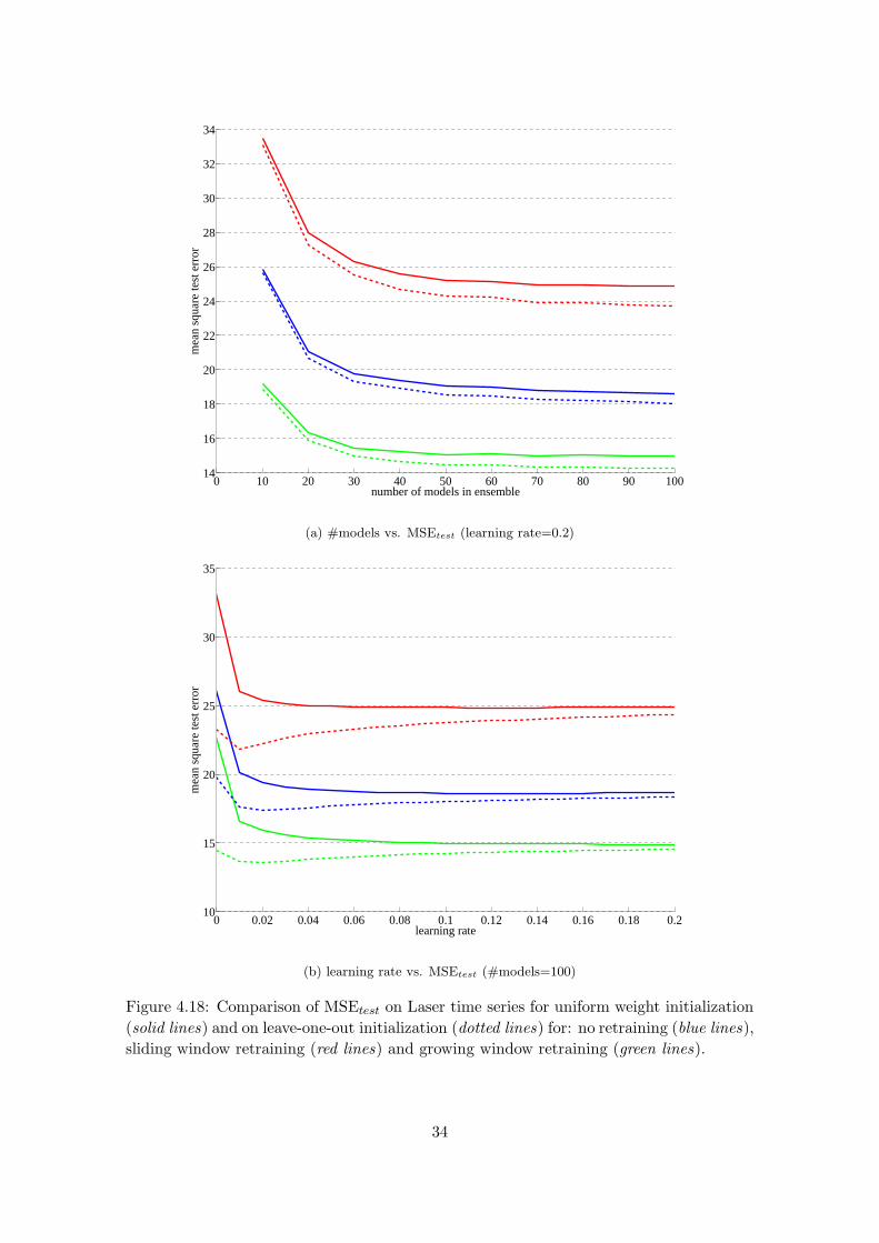
0 10 20 30 40 50 60 70 80 90 10014

16

18

20

22

24

26

28

30

32

34


mea

n sq

uare

test

err

or


0 0.02 0.04 0.06 0.08 0.1 0.12 0.14 0.16 0.18 0.210

15

20

25

30

35

learning rate

mea

n sq

uare

test

err

or


Figure 4.18: Comparison of MSEtest on Laser time series for uniform weight initialization

(solid lines) and on leave-one-out initialization (dotted lines) for: no retraining (blue lines),

sliding window retraining (red lines) and growing window retraining (green lines).

34

0 10 20 30 40 50 60 70 80 90 100440

460

480

500

520

540

560

580


mea

n sq

uare

test

err

or


0 0.02 0.04 0.06 0.08 0.1 0.12 0.14 0.16 0.18 0.2440

460

480

500

520

540

560

580

learning rate

mea

n sq

uare

test

err

or


Figure 4.19: Comparison of MSEtest on Quebec time series for uniform weight initialization

(solid lines) and on leave-one-out initialization (dotted lines) for: no retraining (blue lines),

sliding window retraining (red lines) and growing window retraining (green lines).

35

Santa Fe Laser Data

In Figure 4.20, the average running times of the various ensemble types are shown. From

Figure 4.20a, it can be seen that in case we are not retraining the models, the extra

ensemble weight initialization roughly doubles the running time. This makes sense, since

in the computation of the leave-one-out error we need to compute the HAT matrix (see

Section 2.2), which is quite similar to the pseudo-inverse of the hidden layer output matrix

H† that is needed for training the model (see Section 2.5).

0 20 40 60 80 1000

5

10

15

20

25

30

35

40


time

(s)

(a)

0 20 40 60 80 1000

1000

2000

3000

4000

5000

6000


time

(s)

(b)

Figure 4.20: Running time of the ensemble on Laser series for varying numbers of models

for uniform initialization (solid lines), LOO initialization (dotted lines), no retraining (blue

lines), sliding window retraining (red lines) and growing window retraining (green lines).

Figure 4.20b shows the average running times for the various ensemble types. We see

that when the models are retrained, the running time is a lot higher and retraining on

a growing window is faster than retraining on a sliding window. This makes sense, since

every iteration we need to both add and remove a sample, instead of just add a sample.

When retraining, every individual model is effectively retrained 9000 times. Although this

might seem excessive, the incremental learning of the model as described in Section 3.2.3

helps a lot. If we compare the average time each model adds to the running time of the

ensemble in Table 4.2, then we see that retraining with incremental learning is 10 to 12

times faster than retraining without incremental learning.

Furthermore, if we are retraining the models, we see that the time needed for the leave-

one-out initialization of the ensemble weights does not make much of a difference anymore.

Table 4.2: Average time (s) a single model adds to running time of ensemble on Laser

retraining

initialization incr. learning none sliding growing

uniform yes 0.23 51.01 41.01

uniform no - 496.55 501.38

leave-one-out yes 0.35 50.91 38.99

leave-one-out no - 499.46 512.3

36

Quebec Births

In Figure 4.21, the average running times of the various ensemble types are shown. The

results are similar to the results observed in the Laser time series, but the running times

are slightly faster due to the fact that the time series only has 5000 values instead of 10000.

0 20 40 60 80 1000

5

10

15

20

25

30


time

(s)

(a)

0 20 40 60 80 1000

500

1000

1500

2000

2500

number of models in ensembletim

e (s

)

(b)

Figure 4.21: Running time of the ensemble on Quebec series for varying numbers of models

for uniform initialization (solid lines), LOO initialization (dotted lines), no retraining (blue

lines), sliding window retraining (red lines) and growing window retraining (green lines).

The average time each model adds to the running time of the ensemble is compared in

Table 4.3. The results are comparable to what we saw with the Laser time series. Namely,

we observe great speedups by the incremental learning, and growing window retraining is

performing slightly faster than sliding window retraining.

Table 4.3: Average time (s) a single model adds to running time of ensemble on Quebec

retraining

initialization incr. learning none sliding growing

normal yes 0.15 22.37 18.02

normal no - 201.82 212.62

leave-one-out yes 0.28 23.21 18.96

leave-one-out no - 205.06 210.51

Least Squares Support Vector Machine

Finally, we run one of the state-of-the-art algorithms, the Least Squares Support Vector

Machine (LS-SVM) [20], for comparison with the adaptive ensemble model of Extreme

Learning Machines in terms of prediction error and running time.

For running the LS-SVM, we use the LS-SVMlab Toolbox [23] by Suykens et al.. We have

to do structural selection of the model, as we earlier described in Section 2.3.2. For this,

we search for the optimal hyperparameters using the built-in grid search, where each of

the hyperparameter candidates is evaluated using 10-fold crossvalidation on the training

set. For an overview of the rest of the used parameters, see Table 4.4.

37

Table 4.4: Parameters used for LS-SVM

parameter value

regressor size 8 (Laser), 14 (Quebec)

#selected variables 5-8 (Laser), 12-14 (Quebec)

initial γ 10

initial σ 0.2

kernel Radial Basis Function (RBF)

trained on first 1000 values

retraining none

parameter optimization function grid search

parameter evaluation function 10-fold crossvalidation

The results of the experiment can be found in table 4.5. In order to get an idea of the

variance and the mean of the result, we perform 10 runs and report the mean and standard

deviation for the measurements.

Table 4.5: LS-SVM Results

time series msetest running time (s)

Laser 18.29 (± 3.38) 800.3 (± 24.0)

Quebec 863.22 (± 65.91) 1536.7 (± 18.4)

The LS-SVM is able to achieve good prediction performance for the Laser time series

(lowest mean square prediction error recorded was 13.53), at reasonable running times.

Unfortunately, the variance is quite high compared to the variance of prediction error the

ensemble of ELMs.

For the Quebec time series, the LS-SVM performs a lot worse than the ensemble of ELMs

(lowest mean square prediction error was 803.08). Also, optimizing the model structure

takes a lot longer for this time series. We expect that this is because of the size of the larger

regressor size and the larger amount of time that needs to be spent in the crossvalidation.

38

Chapter 5

Discussion

In this chapter, we will discuss the results of the experiments in greater detail and we will

try to put the results in perspective.

First, we discuss the influence of the different parameters that we varied in the various

experiments. Then, we compare the adaptive ensemble models with the LS-SVM and

further discuss in what context the adaptive ensemble models can be used, in light of

these results.

5.1 Effect of Number of Models

In all experiments, we can clearly see that combining multiple models into a single ensemble

model results in better performance than each of the models by itself. Also, adding more

models generally results in better expected prediction performance. Furthermore, the

more models are added to the ensemble, the smaller the variance on the performance

becomes.

While more experiments would be required to get insight in the exact relation between

the test error of the individual models and the test error of the ensemble of these models,

it seems that for the models used in prediction on the Laser time series, we get the most

dramatic improvement by ensembling them. In this case, an ensemble of 100 models

achieved a test error of 17.72, while the best model from that ensemble only was able to

achieve a test error of 33.85. For an ensemble of 100 models on the Quebec time series,

we observed a test error of 567.96 for the ensemble, while the best individual model from

that ensemble achieved a test error of 602.95.

5.2 Effect of Learning Rate

For both time series, we observed that the adaptive ensemble model improves on the

ensemble model that just takes the average of the models (i.e. learning rate of 0). Fur-

thermore, the effect of the learning rate seems to be the same across ensembles of different

numbers of models, as can be seen in Figure 5.1.

For both time series, we see that with increasing learning rate, the test error quickly drops

and then flattens out.

For the Laser time series, we see larger improvements than for the Quebec time series,

39

0 0.05 0.1 0.15 0.215

20

25

30

35

learning rate

mea

n sq

uare

test

err

or

(a)

0 0.05 0.1 0.15 0.2545

550

555

560

565

570

575

580

learning rate

mea

n sq

uare

test

err

or

(b)

Figure 5.1: MSEtest as a function of learning rate for (a) Laser time series and (b) Quebec

time series for 10 models (dashed line) and 100 models (solid line).

suggesting that for the ensembles used in prediction on the Laser time series it is more

important that we adapt the weights of the ensemble, such that good models get higher

weight, and vice versa.

Looking at the distribution of the test error in for example Figure 4.11, we indeed see

that there are a number of significantly worse models, which should be ’tuned’ out of the

ensemble as quickly as possible for optimal performance (i.e. the weight with which they

contribute to the ensemble should be reduced).

For the Quebec time series there are no significantly worse models and we observe a less

dramatic increase of performance by increasing the learning rate, giving further evidence

of the relation between the distribution of the test error of individual models and the effect

of learning rate on the performance of the ensemble.

In both time series we observe an optimal learning rate of about 0.1 when using uniform

ensemble weight initialization. Because this seems to hold for all numbers of models in

the ensemble, it seems to be a robust strategy to choose the number of models high and

set the learning rate to 0.1.

When using leave-one-out initialization however, the optimal learning rate seems to be a

lot lower (in case of the Laser time series), or slightly higher (in case of the Quebec time

series). In all cases, a learning rate of 0.1 still gives good performance though.

5.3 Effect of the Leave-one-out Weight Initialization

In Experiment 3, the leave-one-out weight initialization of the ensemble weights was in-

vestigated.

As can be seen from Figure 4.18, for the Laser time series the prediction performance of

the ensemble is improved for any number of models.

We especially see large improvements for the lower learning rates. The leave-one-out

initialization is effective at selecting those models that have good prediction performance

and effectively ’tunes out’ those models that have bad performance, leading to better

prediction performance of the ensemble. The optimal learning rate for the Laser time

40

series is about 0.01 for the leave-one-out weight initialization, and is about 0.1 for the

uniform weight initialization.

More experiments are needed to find out what exactly influences the value of the optimal

learning rate. However, based on these experiments, we suspect that there are at least the

following two factors that influence the optimal learning rate:

• the distribution of the test errors of the individual models: if we have particularly

bad models in the ensemble, then it is beneficial to quickly reduce the weights of

these models as earlier discussed in Section 5.2.

• the local (in time) biases of the individual models: ideally models have randomly

distributed errors [16]. In practice however, within small time intervals, a model

will locally overestimate or underestimate the true value of the time series and make

larger errors than it makes on average. A small learning rate can help in this case

to compensate for the local biases of the models and improve the performance of

the ensemble. Although more experiments are needed to verify this, we think this

could be a possible explanation for the relatively small optimal learning rate in

leave-one-out initialization of the ensemble weights.

Interestingly, for the Quebec time series, the leave-one-out weight initialization results in

worse performance than the uniform weight initialization. We imagine there could be two

possible causes for this:

• nonstationarity of the time series: the models that have good performance on the

beginning of the time series do not necessarily perform well on the later parts of the

time series. Therefore, starting with uniform ensemble weights could be a better

strategy than using estimates of the generalization performance of the individual

models based on their leave-one-out output on the training set.

• distribution of the test errors of the individual models: as can be seen from for

example Figure 4.19, the models all have quite similar test error. Because of this,

there is not so much need for model selection as was the case with the Laser time

series. Furthermore, as we saw in Section 2.4 on ensemble models, the improvement

of the performance of ensemble models relies on the uncorrelatedness of the errors of

the individual models. Therefore, even if models have relatively large error, adding

them to the ensemble can improve accuracy of the ensemble. However, since the

leave-one-out initialization of the ensemble weights assigns small weight to those

models with large error, this could have a negative impact on the accuracy of the

ensemble.

Again, more experiments would be needed to find out how these different factors exactly

contribute to the performance of the ensemble.

5.4 LS-SVM and Performance Considerations

As we can see in Experiment 4, ELMs are extremely fast to train and they can also be

retrained at every time step in reasonable time, thanks to the possibility of incrementally

training them on a sliding or a growing window. That is, being able to add a sample to the

41

training set or removing a sample from the training set and obtaining the newly trained

model from the current model, without completely having to retrain it. It is also worth

mentioning that it is possible to improve the performance by caching the outputs of the

hidden layer for each input, since these are typically needed multiple times.

Of course, the good performance of the models has little meaning if the models do not

have good prediction performance, so therefore we compare the performance with the

performance of Least Squares Support Vector Machines (LS-SVM) [20].

5.4.1 Comparing models

It should be said in advance that comparisons between methods that one is not an expert

in, do not necessarily show the maximum performance of an algorithm. If you have been

working with a certain algorithm for a long time and have a lot of experience with it, you

probably have a better idea on how to get best performance in a certain problem. With

this in mind we proceed to the comparison with LS-SVM.

The settings we used in the experiment for training the LS-SVM are quite common settings

to use in regression problems [20, 24] and should give a good indication of the performance

we would get in the typical use of the LS-SVM. Note that because of the long running time

of the LS-SVM, we did not include any experiments where the LS-SVM is retrained. Here,

we are mostly interested in how the adaptive ensemble method compares in prediction

performance on a typical stationary regression problem. It would be interesting to further

investigate how the LS-SVM can be adapted for fast retraining and for application in

nonstationary time series, but this is something that falls outside the scope of this thesis.

For a fair comparison of the LS-SVM and the adaptive ensemble model of ELMs, we

made sure that both methods have the same information to work with, by using the same

settings for the regressor size and the amount of selected variables. While these potentially

are not the most optimal settings, this holds for both methods so even if we do not get

maximum performance, it should be a fair comparison.

5.4.2 Comparison on Laser Time Series

For the Laser time series, the LS-SVM achieved an average mean square test error of

18.29, with a standard deviation of 3.38 across the different runs. On average a run took

800.3 seconds to complete. As can be seen in Figure 4.18, Figure 4.6b and Appendix A

and B, an ensemble model of 100 ELMs without retraining and learning rate of 0.1 takes

about 23 seconds to run with uniform weight initialization, and achieves an average mean

square error of 18.63, with a standard deviation of 0.93. So, it has only a little bit worse

prediction performance while being about 32 times faster. Furthermore, the standard

deviation is a lot lower so the achieved prediction performance is more consistent.

Of course, we could add extra models to the ensemble to achieve better prediction perfor-

mance, but we expect only little improvement from this and it would be better to spend

time on for example leave-one-out weight initialization of the ensemble.

If we add leave-one-out weight initialization to the ensemble, then the same ensemble of

100 ELMs (no retraining, learning rate 0.1) achieves an average mean square error of 18.03,

with a standard deviation of 0.94, while still being 23 times faster than the LS-SVM.

42

5.4.3 Comparison on Quebec Time Series

As can be seen from the results of Experiment 4, the LS-SVM performs quite badly on the

Quebec time series and only achieves an average test error of time series 863.22 and takes

1536 seconds to run on average. In the same time, it would be possible to run an ensemble

of about 60 to 70 ELMs (see Figure 4.19) which would achieve a test error around 460

(see Figure 4.18).

From these results, we can conclude that the LS-SVM as it was used is not suited for

prediction on nonstationary time series, and that the adaptive ensemble seems to perform

nicely for nonstationary time series. Note that even when we do not retrain the individual

models, the adaptive ensemble model still performs a lot better than the LS-SVM.

Since we could not make a good comparison with LS-SVM on the nonstationary time series,

it would be interesting to see how the adaptive ensemble compares in terms of prediction

performance and running time with other methods that are suitable for prediction on

nonstationary time series.

43

44

Chapter 6

Future Work

No matter what area of research, there are always more questions to ask than one can

answer, as was the case with this thesis. In this chapter we will give several suggestions

for promising research directions that could be worth exploring as a continuation of this

work.

6.1 Explore Links with Other Fields

In this thesis we have looked at ensemble models of Extreme Learning Machines for one-

step ahead time series prediction, mostly from an experimental point of view.

At a rather late stage in the process, the links between this work and the field of adaptive

filtering and signal processing [25, 26] became clear. The theory behind adaptive filters is

well developed and adaptive filters can for example be used for noise reduction of signals,

echo cancellation and signal prediction. Especially the theory for signal prediction with

adaptive filters seems very useful for one-step ahead prediction.

Further exploration in applying techniques and theorems from adaptive filtering and signal

processing to the work discussed in this thesis definitely seems useful. I would even say that

it is required, since the links between both fields are quite strong and essentially solve the

same problem: approximating a target signal as good as possible based on various kinds

of input signals.

6.2 Improving on Input Selection

Even though the models presented in this thesis achieve good performance by choosing

sensible regressor sizes and input variables, there is probably a lot to be gained from doing

input variable selection. See for example [27] for an overview of input variable selection

methods and see [28] and [29] for information on the Delta test that can be used for

variable selection and data preprocessing.

6.3 Improving Individual Models

Another possibility is to improve on the individual models in the ensemble. For example,

one could use some criterion like the Aikaike information criterion (AIC), or Bayesian

45

information criterion (BIC) [4] to estimate the optimal number of hidden neurons to use

in the ELM.

Another natural extension of the current work is to use OP-ELM [24] instead of ELM,

which are basically ELMs where the least significant neurons are pruned for better gener-

alization.

6.4 Improving Ensemble Model

In changing the weights of the ensemble model, currently only the square errors are used,

so we are effectively losing the information about the sign of the error. This works great

and the models tend to have sufficiently uncorrelated error to be ensembled in an effective

way. However, we could possibly improve on this by explicitly taking into account the sign

of the error, and make sure that they are sufficiently uncorrelated. That is, we could try to

make sure that there is a certain degree of diversity between the models in the ensemble.

It is shown in [8] that strategies like bagging [10] or boosting [11] can improve ensemble

accuracy. In both these strategies each of the individual models is trained on a modified

version of the training set, which introduces diversity between the models.

Another interesting extension of the current work would be to use the estimated leave-

one-out output of the models at all times as a basis for the weights of the ensemble, and

not just as an initialization. While it might increase the required computational time,

this could potentially lead to a better combination of the individual models, with a better

prediction performance of the ensemble model as a result.

6.5 Other Degrees of Adaptivity

In the current method the models that are part of the ensemble are never removed, and

only the weight with which they contribute is changed. If a model consistently gives bad

performance though, we might as well remove it and reduce the computational time of the

ensemble or add another model instead.

A possible implementation would be one that we initially had in mind when starting this

work, but unfortunately never had time to implement. One could for example create a

hybrid version of the current method and an evolutionary algorithm in the form of a multi-

agent simulation. The models would then be seen as agents, and would be evaluated for

fitness and compete with other agents for a limited energy resource. At each time step,

the agents would gain or lose a certain amount of energy as a result of this. In case an

agent runs out of energy, it dies and in case it reaches a certain level of energy it replicates

with small variation of the parameters.

In the short term, this simulation would behave similar to the one described in this thesis,

and over the long term the models will hopefully adapt to the problem at hand and be able

to determine the model parameters that work best. An example use of such a simulation

could be to obtain pre-adapted models for a certain environment or prediction problem.

It would be interesting to see how effective this method would be at producing good

models, and how this method can be used in practice in time series prediction problems.

46

6.6 Parallel implementation

Because of the modular nature of ensemble models, another promising future direction

of the work presented in this thesis is the parallellization of the ensemble models (and

the individual models). The ensemble models can easily be parallelized by executing the

individual models in parallel on different nodes of a cluster. Often, the individual models

themselves can be made faster as well by parallelizing them.

On the one hand, this parallelization will allow faster evaluation of the models, which is

always a desired property of a model. In certain cases, fast evaluation is even a necessary

property of the models. For example, in contexts where there are time constraints on

getting the prediction like the stock market or in control applications.

On the other hand, the faster evaluation of the models will also enable timely evaluation

of larger ensemble models, which could lead to improved prediction quality.

Finally, speeding up the evaluation of the ensemble models and individual models will

allow for more exploratory research. For example, think about running large number of

models, sweeping entire parameter ranges to investigate the effect of a certain parameter

on the performance, or doing exhaustive search on the huge number of model structures

one often has to deal with.

6.7 GPU Computing

Finally, a very promising direction that I hope to continue in myself is parallel computing

using video cards.

Nowadays, video cards are increasing more rapidly in terms of performance than normal

desktop processors, and provide huge amounts of computational power. For example, the

most high-end video card at the moment, the NVidia GTX295, has 2 Graphics Processing

Units (GPUs) which amount to a total of 1790 GFlops of computational power. Compared

to the approximately 50 GFlops for a high-end Intel i7 processor, this is huge.

In 2007, NVIDIA (one of the two main manufacturers of video cards) introduced CUDA [30],

which is an API that can be used to run your code on the highly-parallel GPUs.

Examples of succesful applications of CUDA can be found at [30], and include examples

from biotechnology [31], linear algebra [32], molecular dynamics simulations [33] and ma-

chine learning [34]. Depending on your application, speedups of 20-300 times are possible

by executing code on a single GPU instead of the CPU, and by using multiple GPUs you

should be able to obtain even higher speedups.

Thanks to funding from the Adaptive Informatics Research Centre (AIRC), we have been

able to design and build a desktop computer with three of these GTX295 video cards. This

particular setup gives a total amount of raw computational power of over 5 TeraFlops.

This is comparable to the computational power of a small cluster, and personally, I am

very much looking forward to see what can be achieved with this machine.

47

48

Chapter 7

Conclusions

In this thesis, we have presented an adaptive ensemble model of Extreme Learning Ma-

chines (ELMs) for use in one-step ahead prediction. The model has been analyzed on both

stationary and nonstationary time series, in terms of performance and prediction error.

The performed experiments provide a thorough overview of the influence of the various

parameters of the model, and show that in prediction on both stationary and nonstation-

ary time series, the adaptive ensemble method is able to achieve a prediction accuracy

comparable to or better than a state-of-the-art methods like the Least Squares Support

Vector Machine. Furthermore, the results suggest a robust strategy for choosing the pa-

rameters of the method (i.e. choose number of models sufficiently large and choose learning

parameter α = 0.1).

An added advantage besides the good prediction performance of the presented model, is

that it is able to achieve this prediction performance while remaining adaptive, and does

so at low computational cost.

Because of its modular nature, the presented ensemble model can easily be parallelized,

Therefore, even though the presented model already has low computational cost, it is

possible to speed it up even further quite easily.

Besides parallelizing, a large number of possible continuations for this work has been

provided. For example, a more thorough statistical analysis of the model, in order to

determine the best strategy for optimizing the parameters.

Overall, the results suggest that the adaptive ensemble model presented and analyzed

in this thesis, makes an excellent candidate for application in both a stationary and a

nonstationary context.

Finally, the simplicity and effectivity of the model, together with the large number of

possible aspects to investigate make it a nice subject to do research on. I certainly found

it an interesting research topic. Although at times it was frustrating when something was

not working as expected, I had a lot of fun doing the research for this thesis, and hope to

be able to further continue with this subject in the future.

49

50

Chapter 8

Bibliography

8.1 References

[1] A. Sorjamaa, J. Hao, N. Reyhani, Y. Ji, A. Lendasse, Methodology for long-term

prediction of time series., Neurocomputing 70 (16-18) (2007) 2861–2869.

[2] G. Simon, A. Lendasse, M. Cottrell, J.-C. Fort, M. Verleysen, Time series forecasting:

Obtaining long term trends with self-organizing maps, Pattern Recognition Letters

26 (12) (2005) 1795 – 1808.

[3] S. Haykin, Neural Networks: A Comprehensive Foundation, Prentice Hall, Upper

Saddle River, NJ, 1999, 2nd edition.

[4] C. M. Bishop, Pattern Recognition and Machine Learning (Information Science and

Statistics), Springer-Verlag New York, Inc., Secaucus, NJ, USA, 2006.

[5] C. R. Rao, S. K. Mitra, Generalized Inverse of Matrices and Its Applications, John

Wiley & Sons Inc, 1972.

[6] K. Hornik, M. B. Stinchcombe, H. White, Multilayer feedforward networks are uni-

versal approximators., Neural Networks 2 (5) (1989) 359–366.

[7] B. Efron, R. J. Tibshirani, An Introduction to the Bootstrap, Chapman & Hall/CRC,

1994.

[8] L. I. Kuncheva, Classifier ensembles for changing environments, MCS (2004) 1–15.

[9] L. Hansen, P. Salamon, Neural network ensembles, Pattern Analysis and Machine

Intelligence, IEEE Transactions on 12 (10) (1990) 993–1001.

[10] L. Breiman, Bagging predictors, in: Machine Learning, 1996, pp. 123–140.

[11] R. E. Schapire, Y. Freund, P. Bartlett, W. S. Lee, Boosting the margin: a new

explanation for the effectiveness of voting methods, The Annals of Statistics 26 (1998)

322–330.

[12] R. A. Jacobs, M. I. Jordan, S. J. Nowlan, G. E. Hinton, Adaptive mixtures of local

experts, Neural Computation 3 (1991) 79–87.

51

[13] S. Raudys, I. Zliobaite, The multi-agent system for prediction of financial time series,

Artificial Intelligence and Soft Computing - ICAISC 2006 (2006) 653–662.

[14] G.-B. Huang, Q.-Y. Zhu, C.-K. Siew, Extreme learning machine: Theory and appli-

cations, Neurocomputing 70 (1-3) (2006) 489 – 501.

[15] G.-B. Huang, L. Chen, C. K. Siew, Universal approximation using incremental con-

structive feedforward networks with random hidden nodes., IEEE Transactions on

Neural Networks 17 (4) (2006) 879–892.

[16] R. Myers, Classical and Modern Regression with Applications, 2nd edition, Duxbury,

Pacific Grove, CA, USA, 1990.

[17] G. J. Bierman, Factorization Methods for Discrete Sequential Estimation, Academic

Press, New York, NY, 1977.

[18] A. Sorjamaa, Strategies for the long-term prediction of time series using local models,

Master’s thesis, Helsinki University of Technology (October 14 2005).

[19] G. Bontempi, M. Birattari, H. Bersini, Recursive lazy learning for modeling and

control, in: European Conference on Machine Learning, 1998, pp. 292–303.

[20] J. A. K. Suykens, T. V. Gestel, J. D. Brabanter, B. D. Moor, J. Vandewalle, Least

Squares Support Vector Machines, World Scientific, Singapore, 2002.

[21] A. Weigend, N. Gershenfeld, Time Series Prediction: Forecasting the Future and

Understanding the Past, Addison-Wesley, 1993.

[22] Quebec Births Data: http://www-personal.buseco.monash.edu.au/~hyndman/

TSDL/misc/qbirths.dat.

[23] LS-SVMlab Toolbox Version 1.5: http://www.esat.kuleuven.ac.be/sista/

lssvmlab/.

[24] Y. Miche, A. Sorjamaa, A. Lendasse, OP-ELM: Theory, experiments and a toolbox.,

in: V. Kurkov, R. Neruda, J. Koutnk (Eds.), ICANN (1), Vol. 5163 of Lecture Notes

in Computer Science, Springer, 2008, pp. 145–154.

[25] M. H. Hayes, Statistical Digital Signal Processing and Modeling, Wiley, 1996.

[26] S. Haykin, Adaptive Filter Theory (4th Edition), Prentice Hall, 2001.

[27] J. Tikka, Input variable selection methods for construction of interpretable regression

models, Doctoral dissertation, TKK Dissertations in Information and Computer Sci-

ence TKK-ICS-D11, Helsinki University of Technology, Faculty of Information and

Natural Sciences, Department of Information and Computer Science, Espoo, Finland

(December 2008).

[28] E. Eirola, E. Liitiainen, A. Lendasse, F. Corona, M. Verleysen, Using the delta test

for variable selection, in: Proc. of ESANN 2008 European Symposium on Artificial

Neural Networks, 2008, pp. 25–30.

52

[29] F. Mateo, D. Sovilj, R. G. Girons, A. Lendasse, Rcga-s/rcga-sp methods to mini-

mize the delta test for regression tasks., in: J. Cabestany, F. Sandoval, A. Prieto,

J. M. Corchado (Eds.), IWANN (1), Vol. 5517 of Lecture Notes in Computer Science,

Springer, 2009, pp. 359–366.

[30] NVidia CUDA Zone: http://www.nvidia.com/object/cuda_home.html.

[31] M. Schatz, C. Trapnell, A. Delcher, A. Varshney, High-throughput sequence alignment

using graphics processing units, BMC Bioinformatics 8 (1).

[32] V. Volkov, J. W. Demmel, Benchmarking gpus to tune dense linear algebra, in: SC

’08: Proceedings of the 2008 ACM/IEEE conference on Supercomputing, IEEE Press,

Piscataway, NJ, USA, 2008, pp. 1–11.

[33] W. Liu, B. Schmidt, G. Voss, W. Muller-Wittig, Accelerating molecular dynamics

simulations using graphics processing units with cuda, Computer Physics Communi-

cations In Press, Corrected Proof.

[34] B. Catanzaro, N. Sundaram, K. Keutzer, Fast support vector machine training and

classification on graphics processors, in: Proceedings of the 25th International Con-

ference on Machine Learning (ICML 2008), Helsinki, Finland, 2008, pp. 104–111.

53

54

Appendix A

Santa Fe Laser Data Errors

uniform initialization

#models none slide grow

10 25.879 33.484 19.162

20 21.084 27.977 16.327

30 19.756 26.327 15.456

40 19.382 25.573 15.238

50 19.057 25.218 15.075

60 18.971 25.132 15.09

70 18.78 24.916 14.994

80 18.756 24.956 15.033

90 18.696 24.901 14.994

100 18.63 24.863 14.993

Table A.1: Average prediction error on Santa Fe Laser Data (learning rate=0.1)

leave-one-out initialization


10 25.652 33.091 18.881

20 20.649 27.258 15.886

30 19.328 25.544 14.975

40 18.909 24.704 14.669

50 18.555 24.307 14.461

60 18.474 24.2 14.458

70 18.274 23.901 14.339

80 18.207 23.877 14.333

90 18.123 23.792 14.27

100 18.023 23.743 14.245

Table A.2: Average prediction error on Santa Fe Laser Data (learning rate=0.1)

55

learning rate uniform initialization loo initialization

none slide grow none slide grow

0 26.113 33.155 22.68 19.83 23.298 14.445

0.01 20.109 26.009 16.586 17.625 21.865 13.658

0.02 19.424 25.383 15.915 17.384 22.266 13.6

0.03 19.096 25.14 15.577 17.465 22.649 13.693

0.04 18.915 25.018 15.375 17.583 22.928 13.807

0.05 18.808 24.951 15.248 17.69 23.133 13.91

0.06 18.739 24.915 15.163 17.778 23.297 13.999

0.07 18.694 24.893 15.102 17.853 23.434 14.075

0.08 18.664 24.878 15.056 17.917 23.55 14.14

0.09 18.643 24.868 15.021 17.973 23.652 14.196

0.10 18.63 24.863 14.993 18.023 23.743 14.245

0.11 18.623 24.859 14.972 18.068 23.826 14.289

0.12 18.619 24.857 14.955 18.109 23.9 14.328

0.13 18.619 24.857 14.941 18.147 23.969 14.363

0.14 18.621 24.858 14.931 18.182 24.033 14.395

0.15 18.625 24.862 14.924 18.215 24.093 14.425

0.16 18.631 24.866 14.918 18.247 24.149 14.452

0.17 18.638 24.872 14.914 18.277 24.201 14.477

0.18 18.646 24.879 14.911 18.306 24.25 14.501

0.19 18.655 24.888 14.91 18.334 24.298 14.523

0.20 18.665 24.897 14.909 18.361 24.343 14.544

Table A.3: Average prediction error on Santa Fe Laser Data (#models=100)

56

Appendix B

Quebec Birth Data Errors

uniform initialization


10 568.75 468.69 464.56

20 557.77 459.08 460.54

30 553.87 455.39 458.92

40 552.22 453.99 458.44

50 551.5 453.27 458.11

60 551 452.77 458.05

70 550.43 452.41 457.93

80 550.06 451.9 457.62

90 549.16 451.77 457.62

100 548.15 451.6 457.45

Table B.1: Average prediction error on Quebec Births (learning rate=0.1)

leave-one-out initialization


10 569.37 469.21 465.02

20 558.26 459.59 460.96

30 554.38 455.79 459.31

40 552.74 454.33 458.84

50 551.97 453.66 458.51

60 551.58 453.21 458.46

70 550.94 452.88 458.31

80 550.6 452.4 458.05

90 549.65 452.28 458.04

100 548.59 452.08 457.83

Table B.2: Average prediction error on Quebec Births (learning rate=0.1)

57

learning rate uniform initialization loo initialization

none slide grow none slide grow

0 566.86 452.5 460.02 574.18 459.02 462.31

0.01 556.88 451.96 459.13 564.51 456.97 461.28

0.02 552.86 451.66 458.55 558.22 455.48 460.46

0.03 550.86 451.54 458.19 554.29 454.41 459.8

0.04 549.7 451.5 457.95 551.91 453.65 459.28

0.05 548.99 451.49 457.77 550.48 453.11 458.87

0.06 548.56 451.5 457.65 549.62 452.73 458.55

0.07 548.3 451.52 457.57 549.11 452.47 458.3

0.08 548.16 451.54 457.51 548.81 452.28 458.1

0.09 548.12 451.57 457.47 548.65 452.16 457.95

0.10 548.15 451.6 457.45 548.59 452.08 457.83

0.11 548.22 451.63 457.44 548.61 452.03 457.74

0.12 548.34 451.67 457.43 548.66 452 457.68

0.13 548.48 451.71 457.44 548.76 451.99 457.64

0.14 548.65 451.76 457.45 548.88 451.98 457.62

0.15 548.82 451.8 457.47 549.03 451.98 457.6

0.16 549.01 451.85 457.5 549.19 452 457.6

0.17 549.2 451.9 457.52 549.35 452.02 457.6

0.18 549.39 451.95 457.55 549.53 452.04 457.61

0.19 549.58 451.99 457.59 549.7 452.07 457.63

0.20 549.77 452.04 457.62 549.87 452.1 457.65

Table B.3: Average prediction error on Quebec Births (#models=100)

58

Documents

Adaptive Ensemble Models of Extreme Learning Machines for Time