Embed Size (px)
Citation preview
manuscript
Adaptive Distributionally Robust Optimization
Dimitris BertsimasMassachusetts Institute of Technology
Melvyn SimNUS Business School, National University of Singapore
Meilin ZhangSUSS Business School, Singapore University of Social Science
We develop a modular and tractable framework for solving an adaptive distributionally robust linear opti-
mization problem, where we minimize the worst-case expected cost over an ambiguity set of probability
distributions. The adaptive distrbutaionally robust optimization framework caters for dynamic decision mak-
ing, where decisions adapt to the uncertain outcomes as they unfold in stages. For tractability considerations,
we focus on a class of second-order conic (SOC) representable ambiguity set, though our results can easily
be extended to more general conic representations. We show that the adaptive distributionally robust linear
optimization problem can be formulated as a classical robust optimization problem. To obtain a tractable
formulation, we approximate the adaptive distributionally robust optimization problem using linear decision
rule (LDR) techniques. More interestingly, by incorporating the primary and auxiliary random variables of
the lifted ambiguity set in the LDR approximation, we can significantly improve the solutions, and for a
class of adaptive distributionally robust optimization problems, exact solutions can also be obtained. Using
the new LDR approximation, we can transform the distributionally adaptive robust optimization problem to
a classical robust optimization problem with an SOC representable uncertainty set. Finally, to demonstrate
the potential for solving management decision problems, we develop an algebraic modeling package and
illustrate how it can be used to facilitate modeling and obtain high quality solutions for medical appointment
scheduling and inventory management problems.
1. Introduction
Addressing uncertainty in many real world optimization problems has often lead to computation-
ally intractable models. As a result, uncertainty is often ignored in optimization models and this
may lead to poor or even unacceptable decisions when implementing them in practice. We charac-
terize uncertainty as risk, whenever the probability distribution is known, or otherwise as ambiguity
(Knight 1921). Traditionally, mathematical optimization models such as stochastic programming
(see, for instance, Birge and Louveaux 1997, Ruszczynski and Shapiro 2003) are based on the
paradigm of risk and they do not incorporate ambiguity in their decision criteria for optimization.
However, with the growing importance of ambiguity in decision making (see, for instance, Ells-
berg 1961, Hsu et al. 2005), research on ambiguity has garnered considerable interest in various
1
Bertsimas et al.: Adaptive Distributionally Robust Optimization2 Article submitted;
fields including economics, mathematical finance and management science. In particular, robust
optimization is a relatively new approach that deals with ambiguity in mathematical optimization
problems. In classical robust optimization, uncertainty is described by a distribution free uncer-
tainty set, which is typically a conic representable bounded convex set (see, for instance, El Ghaoui
and Lebret 1997, El Ghaoui et al. 1998, Ben-Tal and Nemirovski 1998, 1999, 2000, Bertsimas
and Sim 2004, Bertsimas and Brown 2009, Bertsimas et al. 2011). The key advantage of a robust
optimization model is its computational tractability and it has been successful in providing com-
putationally scalable solutions for a wide variety of management inspired optimization problems.
In evaluating preferences over risk and ambiguity, Gilboa and Schmeidler (1989) propose a deci-
sion criterion that is based on the worst-case expected utility or disutility over an ambiguity set of
probability distributions. Scarf (1958) is first to study a single-product Newsvendor problem where
the precise demand distribution is unknown but is only characterized by its mean and variance.
Subsequently, such models have been extended to minimax stochastic optimization models (see,
for instance, Zackova 1966, Dupacova 1987, Breton and EI Hachem 1995, Shapiro and Kleywegt
2002, Shapiro and Ahmed 2004), and recently to distributionally robust optimization models (see,
for instance, Chen et al. 2007, Chen and Sim 2009, Popescu 2007, Delage and Ye 2010, Xu and
Mannor 2012). In terms of tractable formulations for a wide variety of single stage convex opti-
mization problems, Wiesemann et al. (2014) propose a broad class of ambiguity sets where the
family of probability distributions are characterized by conic representable expectation constraints
and nested conic representable confidence sets.
Dynamic optimization models, where decisions adapt to the uncertain outcomes as they unfold in
stages, typically suffer from the “curse of dimensionality” and are computationally intractable (see,
for instance, Shapiro and Nemirovski 2005, Dyer and Stougie 2006, Ben-Tal et al. 2004). To yield
tractable models, linear decision rule (LDR), where adaptive decisions are restricted to affine func-
tions of the uncertain parameters, was proposed in the early literature of stochastic programming.
However, the technique had been abandoned due to suboptimality of the decision rule (see Garstka
and Wets 1974). Nevertheless, LDR approximation has been revived by Ben-Tal et al. (2004) in
their seminal work on adaptive robust optimization1. Subsequently, Bertsimas et al. (2010) establish
the optimality of LDR approximation in some important classes of adaptive robust optimization
problems. Chen and Zhang (2009) further improve the LDR approximation by extending the affine
dependency to the auxiliary variables associated with the support set. For solving adaptive distri-
butionally robust optimization problems, Chen et al. (2007) propose tractable formulations using
LDR approximation techniques. Henceforth, variants of piecewise-linear decision rule approxima-
tion have been proposed to improve the approximation while maintaining the tractability of the
1 Note that we prefer the term “adaptive” over “adjustable” as used in Ben-Tal et al. (2004).
Bertsimas et al.: Adaptive Distributionally Robust OptimizationArticle submitted; 3
adaptive distributionally robust optimization models. Such approaches include the deflected and
segregated LDR approximation of Chen et al. (2008), the truncated LDR approximation of See
and Sim (2009), and the bideflected and (generalized) segregated LDR approximation of Goh and
Sim (2010). Interestingly, there is also a revival of using LDR approximation for solving multistage
stochastic optimization problems (Kuhn et al. 2011).
For broader impact, a general purpose optimization framework to address a wide variety of
optimization problems should be implementable in software packages where reliable solutions can be
obtained with reasonable computational effort. Compared to deterministic optimization frameworks
such as linear optimization, classical optimization frameworks that deal with uncertainty such as
stochastic optimization and dynamic optimization have been less successful. Software packages that
facilitate robust and distributionally robust optimization modeling have begun to surface in recent
years. Existing toolboxes include YALMIP (Loberg 2012), AIMMS (http://www.aimms.com/),
ROME (Goh and Sim 2009, 2010). and JuMPeR ( http://jumper.readthedocs.org). Of these,
ROME, AIMMS and JuMPeR have also incorporated LDR approximation.
Our contributions to this paper are as follows:
1. We propose a tractable and scalable framework for solving an adaptive distributionally robust
linear optimization problem, where we minimize the worst-case expected cost over a second-order
conic (SOC) representable ambiguity set. We show that adaptive distributionally robust linear
optimization problem can be formulated as a classical robust optimization problem.
2. To obtain tractable formulation, we approximate the adaptive distributionally robust lin-
ear optimization problem using LDR techniques. Depending on the choice of ambiguity set, the
resulting framework is either a linear optimization problem or a second order conic optimization
problem (SOCP), which can be solved efficiently by general purpose commercial grade solvers such
as CPLEX and Gurobi.
3. We show that we can significantly improve the LDR approximation by incorporating the
auxiliary random variable associated with the lifted ambiguity set. This approach outperforms more
sophisticated decision rule approximations developed in Chen and Zhang (2009), Chen et al. (2008),
See and Sim (2009), Goh and Sim (2010). Using the new LDR approximation, we can transform the
adaptive distributionally robust optimization problem to a classical robust optimization problem
with an SOC representable uncertainty set.
4. We demonstrate our approach for addressing a medical appointment scheduling problem as
well as a multiperiod inventory control problem. In these problems, we also show that by incor-
porating partial cross moments information in the ambiguity set, we can significantly improve the
solutions over alternatives found in recent literature where the ambiguity set is only characterized
by marginal moments.
Bertsimas et al.: Adaptive Distributionally Robust Optimization4 Article submitted;
Notations. We use [N ], N ∈N to denote the set of running indices, {1, . . . ,N}. We generally use
bold faced characters such as x∈RN andA∈RM×N to represent vectors and matrices, respectively
and [x]i or xi to denote the ith element of the vector x. We use (x)+ to denote max{x,0}. Special
vectors include 0, 1 and ei which are respectively the vector of zeros, the vector of ones and the
standard unit basis vector. We denote RN,M as the space of all measurable functions from RN
to RM that are bounded on compact sets. We use P0(RI) to represent the set of all probability
distributions on RI . A random variable, z is denoted with a tilde sign and we use z ∼ P, P∈P0(RI)
to define z as an I dimensional random variable with probability distribution P. We denote EP[·]as the expectation over the probability distribution P. For a set W ⊆RI , P [z ∈W] represents the
probability of z being in the set W evaluated on the distribution P.
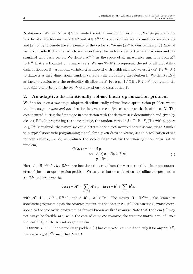
2. An adaptive distributionally robust linear optimization problem
We first focus on a two-stage adaptive distributionally robust linear optimization problem where
the first stage or here-and-now decision is a vector x ∈ RN1 chosen over the feasible set X. The
cost incurred during the first stage in association with the decision x is deterministic and given by
c′x, c∈RN1 . In progressing to the next stage, the random variable z ∼ P, P∈P0(RI) with support
W ⊆RI1 is realized; thereafter, we could determine the cost incurred at the second stage. Similar
to a typical stochastic programming model, for a given decision vector, x and a realization of the
random variable, z ∈W, we evaluate the second stage cost via the following linear optimization
problem,Q(x,z) = min d′y
s.t. A(z)x+By≥ b(z)
y ∈RN2 .
(1)
Here, A∈RI1,M×N1 , b∈RI1,M are functions that map from the vector z ∈W to the input param-
eters of the linear optimization problem. We assume that these functions are affinely dependent on
z ∈RI1 and are given by,
A(z) =A0 +∑k∈[I1]
Akzk, b(z) = b0 +∑k∈[I1]
bkzk,
with A0,A1, ...,AI1 ∈ RM×N1 and b0,b1, ...,bI1 ∈ RM . The matrix B ∈ RM×N2 , also known in
stochastic programming as the recourse matrix, and the vector d∈RN2 are constants, which corre-
spond to the stochastic programming format known as fixed recourse. Note that Problem (1) may
not aways be feasible and, as in the case of complete recourse, the recourse matrix can influence
the feasibility of the second stage problem.
Definition 1. The second stage problem (1) has complete recourse if and only if for any t∈RM ,
there exists y ∈RN2 such that By≥ t.
Bertsimas et al.: Adaptive Distributionally Robust OptimizationArticle submitted; 5
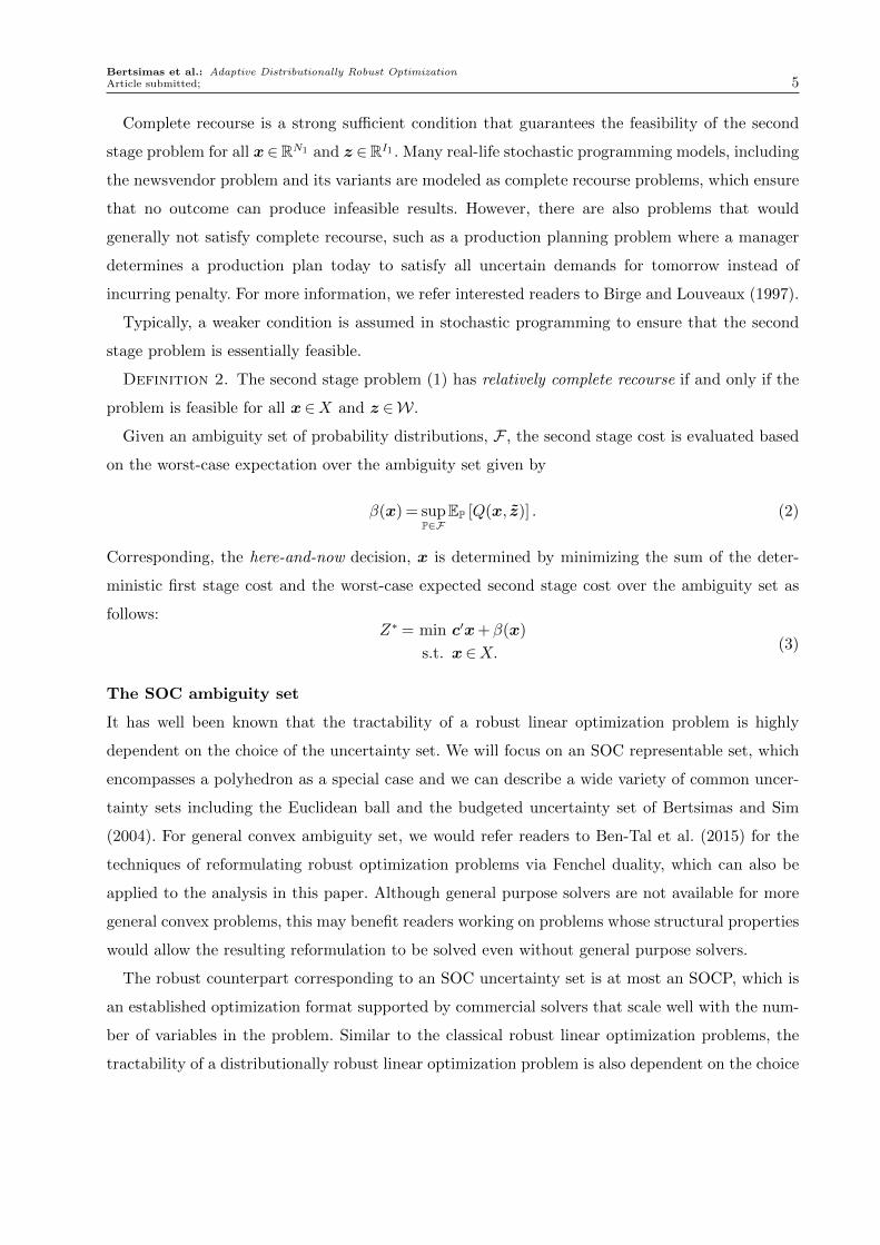
Complete recourse is a strong sufficient condition that guarantees the feasibility of the second
stage problem for all x∈RN1 and z ∈RI1 . Many real-life stochastic programming models, including
the newsvendor problem and its variants are modeled as complete recourse problems, which ensure
that no outcome can produce infeasible results. However, there are also problems that would
generally not satisfy complete recourse, such as a production planning problem where a manager
determines a production plan today to satisfy all uncertain demands for tomorrow instead of
incurring penalty. For more information, we refer interested readers to Birge and Louveaux (1997).
Typically, a weaker condition is assumed in stochastic programming to ensure that the second
stage problem is essentially feasible.
Definition 2. The second stage problem (1) has relatively complete recourse if and only if the
problem is feasible for all x∈X and z ∈W.
Given an ambiguity set of probability distributions, F , the second stage cost is evaluated based
on the worst-case expectation over the ambiguity set given by
β(x) = supP∈F
EP [Q(x, z)] . (2)
Corresponding, the here-and-now decision, x is determined by minimizing the sum of the deter-
ministic first stage cost and the worst-case expected second stage cost over the ambiguity set as
follows:Z∗ = min c′x+β(x)
s.t. x∈X. (3)
The SOC ambiguity set
It has well been known that the tractability of a robust linear optimization problem is highly
dependent on the choice of the uncertainty set. We will focus on an SOC representable set, which
encompasses a polyhedron as a special case and we can describe a wide variety of common uncer-
tainty sets including the Euclidean ball and the budgeted uncertainty set of Bertsimas and Sim
(2004). For general convex ambiguity set, we would refer readers to Ben-Tal et al. (2015) for the
techniques of reformulating robust optimization problems via Fenchel duality, which can also be
applied to the analysis in this paper. Although general purpose solvers are not available for more
general convex problems, this may benefit readers working on problems whose structural properties
would allow the resulting reformulation to be solved even without general purpose solvers.
The robust counterpart corresponding to an SOC uncertainty set is at most an SOCP, which is
an established optimization format supported by commercial solvers that scale well with the num-
ber of variables in the problem. Similar to the classical robust linear optimization problems, the
tractability of a distributionally robust linear optimization problem is also dependent on the choice

Bertsimas et al.: Adaptive Distributionally Robust Optimization6 Article submitted;
of the ambiguity set. In particular the ambiguity set based on information of moments, notwith-
standing its popularity, may not necessarily yield tractable distributionally robust counterparts.
We propose an SOC representable ambiguity set where we restrict only to SOC representation.
For generalization to the ambiguity set of Wiesemann et al. (2014), we refer interested readers to
e-companion EC.5.
Definition 3. An SOC ambiguity set, F is an ambiguity set of probability distributions that
can be expressed as
F =
P∈P0 (RI1)
z ∼ PEP[Gz] =µ
EP[gi(z)]≤ σi ∀i∈ [I2]
P[z ∈W] = 1
(4)
with parameters G ∈ RL1×I1 , µ ∈ RL1 , σ ∈ RI2 , support set W ∈ RI1 and functions gi ∈ RI1,1,
i∈ [I2]. The support set W is an SOC representable set and the epigraph of each gi, i∈ [I2],
epigi = {(z, u)∈RI1 ×R gi(z)≤ u}
is an SOC representable set.
As an illustration, for some given (f , h) ∈ RI1+1, the function g(z) = ((f ′z + h)+)3 is an SOC
representable function because its epigraph is SOC representable given by
epig=
(z, u)∈RI1 ×R ∃v ∈R2 :
v1 ≥ 0, v1 ≥ f ′z+h√v2
1 +(v2−1
2
)2 ≤ v2+12√
v22 +(v1−u
2
)2 ≤ v1+u2
.
The formulation of SOC representable functions is a process that can be automated in an alge-
braic modeling software package. For more information, we refer interested readers to Ben-Tal and
Nemirovski (2001a) for an excellent reference on the algebra of SOC representable functions. The
SOC ambiguity set provides useful and interesting characterization of distributions including:
• Bounds on mean values: EP[z]∈ [µ,µ].
• Upper bound on absolute deviation: EP[|f ′z+h|]≤ σ, for some (f , h)∈RI1+1.
• Upper bound on variance: EP[(f ′z+h)2]≤ σ, for some (f , h)∈RI1+1.
• Upper bound on p-ordered deviation: EP[(|f ′z + h|)p]≤ σ, for some (f , h) ∈ RI1+1 and
some rational p≥ 1.
• Upper bound on semi-variance: EP[((f ′z+h)+)2]≤ σ, for some (f , h)∈RI1+1.
• Approximate upper bound on entropy: EP[exp(f ′z)] ≤ σ, for some f ∈ RI1 . We refer
readers to Ben-Tal and Nemirovski (2001a) for the approximate SOC representation.
• Upper bound on convex piecewise linear function: EP[maxp∈[P ]{f ′pz + hp}] ≤ σ, for
some (fp, hp)∈RI1+1, p∈ [P ].

Bertsimas et al.: Adaptive Distributionally Robust OptimizationArticle submitted; 7
An important class of ambiguity set that could be modeled in the ambiguity set of Wiesemann
et al. (2014) but not ours is the cross moment ambiguity set as follows,
FCM =
P∈P0
(RI1) z ∼ P
EP[z] =µ
EP[(z−µ)(z−µ)′]�Σ
P[z ∈W] = 1
.
Observe that the semidefinite constraint
EP[(z−µ)(z−µ)′]�Σ
is equivalent to the following semi-infinite quadratic constraints
EP[(f ′(z−µ))2]≤ f ′Σf ∀f ∈RI1 . (5)
Hence, as a conservative approximation of the cross moment ambiguity set, we propose the partial
cross moment ambiguity set, which is an SOC ambiguity set as follows:
FPCM =
P∈P0
(RI1) z ∼ P
EP[z] =µ
EP[(f ′k(z−µ))2]≤ f ′kΣfk ∀k ∈ [K]
P[z ∈W] = 1
,
for some choice of parameters f 1, . . . ,fK ∈RI1 . Observe that the approximation never deteriorates
with addition of new vectors, fk, k >K. In our applications to inventory control and appointment
scheduling problems, we will demonstrate how the partial cross moment ambiguity set can yield
tractable models and provide far less conservative solutions than those obtained from the marginal
moment ambiguity set, an ambiguity set that does not consider cross moment information.
As in Wiesemann et al. (2014), we also define the lifted ambiguity set, G that encompasses the
primary random variable z and the lifted or auxiliary random variable u as follows:
G =
P∈P0
(RI1 ×RI2
) (z, u)∼ PEP[Gz] =µ
EP[u]≤σP[(z, u)∈ W
]= 1
, (6)
where W is the lifted support set defined as
W ={
(z,u)∈RI1 ×RI2 z ∈W,g(z)≤u}, (7)
with g(z) = (g1(z), . . . , gI2(z)). Observe that the lifted ambiguity set has only linear expectation
constraints and that the corresponding lifted support set is SOC representable.
Bertsimas et al.: Adaptive Distributionally Robust Optimization8 Article submitted;
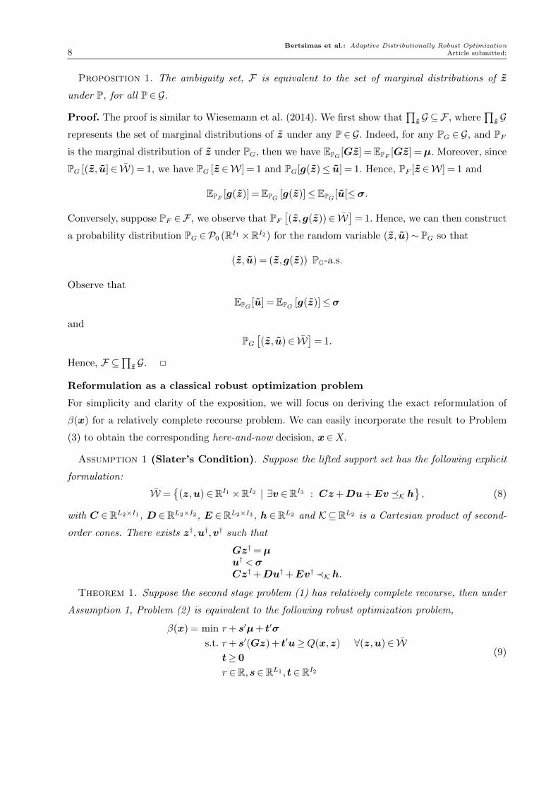
Proposition 1. The ambiguity set, F is equivalent to the set of marginal distributions of z
under P, for all P∈ G.
Proof. The proof is similar to Wiesemann et al. (2014). We first show that∏
z G ⊆F , where∏
z Grepresents the set of marginal distributions of z under any P ∈ G. Indeed, for any PG ∈ G, and PFis the marginal distribution of z under PG, then we have EPG [Gz] =EPF [Gz] =µ. Moreover, since
PG [(z, u]∈ W) = 1, we have PG [z ∈W] = 1 and PG[g(z)≤ u] = 1. Hence, PF [z ∈W] = 1 and
EPF [g(z)] =EPG [g(z)]≤EPG [u[≤σ.
Conversely, suppose PF ∈F , we observe that PF[(z,g(z))∈ W
]= 1. Hence, we can then construct
a probability distribution PG ∈P0 (RI1 ×RI2) for the random variable (z, u)∼ PG so that
(z, u) = (z,g(z)) PG-a.s.
Observe that
EPG [u] =EPG [g(z)]≤σ
and
PG[(z, u)∈ W
]= 1.
Hence, F ⊆∏
z G.
Reformulation as a classical robust optimization problem
For simplicity and clarity of the exposition, we will focus on deriving the exact reformulation of
β(x) for a relatively complete recourse problem. We can easily incorporate the result to Problem
(3) to obtain the corresponding here-and-now decision, x∈X.
Assumption 1 (Slater’s Condition). Suppose the lifted support set has the following explicit
formulation:
W ={
(z,u)∈RI1 ×RI2 | ∃v ∈RI3 : Cz+Du+Ev�K h}, (8)
with C ∈RL2×I1, D ∈RL2×I2, E ∈RL2×I3, h∈RL2 and K⊆RL2 is a Cartesian product of second-
order cones. There exists z†,u†,v† such that
Gz† =µu† <σCz†+Du†+Ev† ≺K h.
Theorem 1. Suppose the second stage problem (1) has relatively complete recourse, then under
Assumption 1, Problem (2) is equivalent to the following robust optimization problem,
β(x) = min r+ s′µ+ t′σ
s.t. r+ s′(Gz) + t′u≥Q(x,z) ∀(z,u)∈ Wt≥ 0
r ∈R,s∈RL1 , t∈RI2
(9)
Bertsimas et al.: Adaptive Distributionally Robust OptimizationArticle submitted; 9
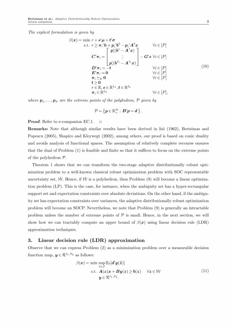
The explicit formulation is given by
β(x) = min r+ s′µ+ t′σs.t. r≥πi′h+pi
′b0−pi′A0x ∀i∈ [P ]
C ′πi =
p′i(b1−A1x)
...p′i(b
I1 −AI1x)
−G′s ∀i∈ [P ]
D′πi =−t ∀i∈ [P ]E′πi = 0 ∀i∈ [P ]πi �K 0 ∀i∈ [P ]t≥ 0r ∈R,s∈RL1 , t∈RI2πi ∈RL2 ∀i∈ [P ],
(10)
where p1, . . . ,pP are the extreme points of the polyhedron, P given by
P ={p∈RM+ : B′p= d
}.
Proof. Refer to e-companion EC.1.
Remarks: Note that although similar results have been derived in Isii (1962), Bertsimas and
Popescu (2005), Shapiro and Kleywegt (2002), among others, our proof is based on conic duality
and avoids analysis of functional spaces. The assumption of relatively complete recourse ensures
that the dual of Problem (1) is feasible and finite so that it suffices to focus on the extreme points
of the polyhedron P.
Theorem 1 shows that we can transform the two-stage adaptive distributionally robust opti-
mization problem to a well-known classical robust optimization problem with SOC representable
uncertainty set, W. Hence, if W is a polyhedron, then Problem (9) will become a linear optimiza-
tion problem (LP). This is the case, for instance, when the ambiguity set has a hyper-rectangular
support set and expectation constraints over absolute deviations. On the other hand, if the ambigu-
ity set has expectation constraints over variances, the adaptive distributionally robust optimization
problem will become an SOCP. Nevertheless, we note that Problem (9) is generally an intractable
problem unless the number of extreme points of P is small. Hence, in the next section, we will
show how we can tractably compute an upper bound of β(x) using linear decision rule (LDR)
approximation techniques.
3. Linear decision rule (LDR) approximation
Observe that we can express Problem (2) as a minimization problem over a measurable decision
function map, y ∈RI1,N2 as follows:
β(x) = min supP∈F
EP[d′y(z)]
s.t. A(z)x+By(z)≥ b(z) ∀z ∈Wy ∈RI1,N2 .
(11)
Bertsimas et al.: Adaptive Distributionally Robust Optimization10 Article submitted;
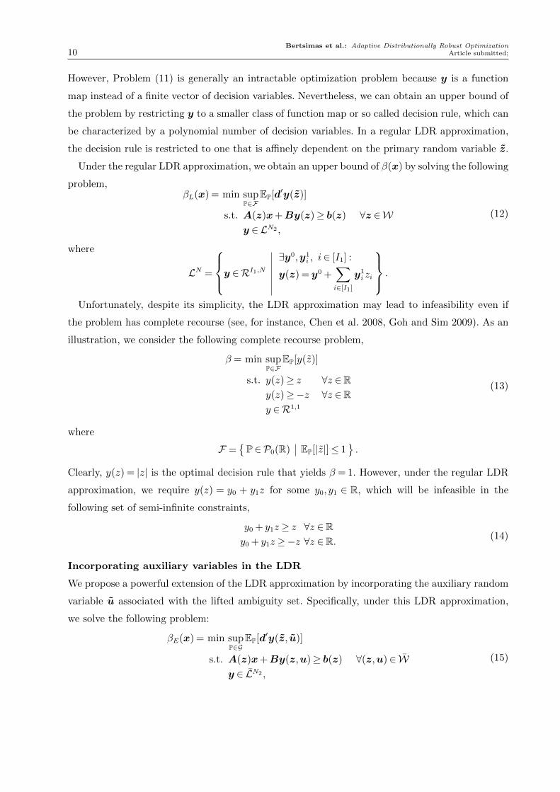
However, Problem (11) is generally an intractable optimization problem because y is a function
map instead of a finite vector of decision variables. Nevertheless, we can obtain an upper bound of
the problem by restricting y to a smaller class of function map or so called decision rule, which can
be characterized by a polynomial number of decision variables. In a regular LDR approximation,
the decision rule is restricted to one that is affinely dependent on the primary random variable z.
Under the regular LDR approximation, we obtain an upper bound of β(x) by solving the following
problem,βL(x) = min sup
P∈FEP[d′y(z)]
s.t. A(z)x+By(z)≥ b(z) ∀z ∈Wy ∈LN2 ,
(12)
where
LN =
y ∈RI1,N∃y0,y1
i , i∈ [I1] :
y(z) = y0 +∑i∈[I1]
y1i zi
.
Unfortunately, despite its simplicity, the LDR approximation may lead to infeasibility even if
the problem has complete recourse (see, for instance, Chen et al. 2008, Goh and Sim 2009). As an
illustration, we consider the following complete recourse problem,
β = min supP∈F
EP[y(z)]
s.t. y(z)≥ z ∀z ∈Ry(z)≥−z ∀z ∈Ry ∈R1,1
(13)
where
F ={P∈P0(R) EP[|z|]≤ 1
}.
Clearly, y(z) = |z| is the optimal decision rule that yields β = 1. However, under the regular LDR
approximation, we require y(z) = y0 + y1z for some y0, y1 ∈ R, which will be infeasible in the
following set of semi-infinite constraints,
y0 + y1z ≥ z ∀z ∈Ry0 + y1z ≥−z ∀z ∈R.
(14)
Incorporating auxiliary variables in the LDR
We propose a powerful extension of the LDR approximation by incorporating the auxiliary random
variable u associated with the lifted ambiguity set. Specifically, under this LDR approximation,
we solve the following problem:
βE(x) = min supP∈G
EP[d′y(z, u)]
s.t. A(z)x+By(z,u)≥ b(z) ∀(z,u)∈ Wy ∈ LN2 ,
(15)
Bertsimas et al.: Adaptive Distributionally Robust OptimizationArticle submitted; 11
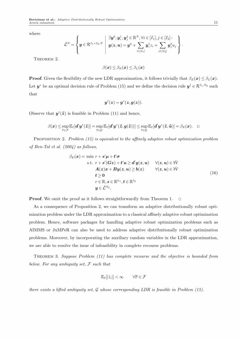
where
LN =
y ∈RI1+I2,N
∃y0,y1i ,y
2j ∈RN ,∀i∈ [I1], j ∈ [I2] :
y(z,u) = y0 +∑i∈[I1]
y1i zi +
∑j∈[I2]
y2juj
.
Theorem 2.
β(x)≤ βE(x)≤ βL(x)
Proof. Given the flexibility of the new LDR approximation, it follows trivially that βE(x)≤ βL(x).
Let y∗ be an optimal decision rule of Problem (15) and we define the decision rule y† ∈RI1,N2 such
that
y†(z) = y∗(z,g(z)).
Observe that y†(z) is feasible in Problem (11) and hence,
β(x)≤ supP∈F
EP[d′y†(z)] = supP∈G
EP[d′y∗(z,g(z))]≤ supP∈G
EP[d′y∗(z, u)] = βE(x).
Proposition 2. Problem (15) is equivalent to the affinely adaptive robust optimization problem
of Ben-Tal et al. (2004) as follows,
βE(x) = min r+ s′µ+ t′σ
s.t. r+ s′(Gz) + t′u≥ d′y(z,u) ∀(z,u)∈ WA(z)x+By(z,u)≥ b(z) ∀(z,u)∈ Wt≥ 0
r ∈R,s∈RL1 , t∈RI2y ∈ LN2 .
(16)
Proof. We omit the proof as it follows straightforwardly from Theorem 1.
As a consequence of Proposition 2, we can transform an adaptive distributionally robust opti-
mization problem under the LDR approximation to a classical affinely adaptive robust optimization
problem. Hence, software packages for handling adaptive robust optimization problems such as
AIMMS or JuMPeR can also be used to address adaptive distributionally robust optimization
problems. Moreover, by incorporating the auxiliary random variables in the LDR approximation,
we are able to resolve the issue of infeasibility in complete recourse problems.
Theorem 3. Suppose Problem (11) has complete recourse and the objective is bounded from
below. For any ambiguity set, F such that
EP[|zi|]<∞ ∀P∈F
there exists a lifted ambiguity set, G whose corresponding LDR is feasible in Problem (15).

Bertsimas et al.: Adaptive Distributionally Robust Optimization12 Article submitted;
Proof. Refer to e-companion EC.2. .
Remarks: Note that the class of ambiguity set depicted in Theorem 3 encompasses any random
variable with finite deviation, i.e., EP[|zi−µi|pi ]<∞ for some µi ∈R, pi ≥ 1, i∈ [I1], since
EP[|zi|]≤EP[|zi−µi|] + |µi| ≤ (EP[|zi−µi|pi ])1/pi + |µi|<∞.
More interestingly, we show in the following result that the new LDR approximation can attain the
optimal objective values for a class of adaptive distributionally robust linear optimization problems.
Theorem 4. Suppose Problem (11) is a complete recourse problem with only one second stage
decision variable, i.e. N2 = 1, then
β(x) = βE(x).
Proof. Refer to e-companion EC.3. .
Remarks: Note that for complete recourse problem with N2 = 1, Problem (9) becomes a tractable
problem since the number of extreme points of the polyhedron P equals to M . Nevertheless,
notwithstanding the simplicity, we are not aware of other types of decision rules that would yield
tight results for this instance.
A natural question is whether we could extend the results of Theorem 3 and 4 to the case of
relatively complete recourse. However, this is not the case as depicted in the following negative
result even for the case of N2 = 1.
Proposition 3. There exists a relatively complete recourse problem with N2 = 1 for which Prob-
lem (15) is infeasible under any LDR that incorporates both the primary and auxiliary random
variables associated with the lifted ambiguity set.
Proof. Consider the following problem
min 0
s.t. y(z)≥ z1− z2 ∀z ∈Wy(z)≥ z2− z1 ∀z ∈Wy(z)≤ z1 + z2 + 2 ∀z ∈Wy(z)≤−z1− z2 + 2 ∀z ∈Wy ∈R2,1
(17)
where
W ={z ∈R2 ‖z‖∞ ≤ 1
}.
Bertsimas et al.: Adaptive Distributionally Robust OptimizationArticle submitted; 13
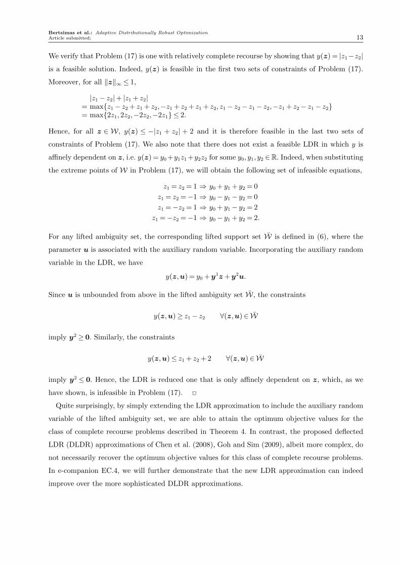
We verify that Problem (17) is one with relatively complete recourse by showing that y(z) = |z1−z2|
is a feasible solution. Indeed, y(z) is feasible in the first two sets of constraints of Problem (17).
Moreover, for all ‖z‖∞ ≤ 1,
|z1− z2|+ |z1 + z2|= max{z1− z2 + z1 + z2,−z1 + z2 + z1 + z2, z1− z2− z1− z2,−z1 + z2− z1− z2}= max{2z1,2z2,−2z2,−2z1} ≤ 2.
Hence, for all z ∈ W, y(z) ≤ −|z1 + z2| + 2 and it is therefore feasible in the last two sets of
constraints of Problem (17). We also note that there does not exist a feasible LDR in which y is
affinely dependent on z, i.e. y(z) = y0 +y1z1 +y2z2 for some y0, y1, y2 ∈R. Indeed, when substituting
the extreme points of W in Problem (17), we will obtain the following set of infeasible equations,
z1 = z2 = 1 ⇒ y0 + y1 + y2 = 0
z1 = z2 =−1 ⇒ y0− y1− y2 = 0
z1 =−z2 = 1 ⇒ y0 + y1− y2 = 2
z1 =−z2 =−1 ⇒ y0− y1 + y2 = 2.
For any lifted ambiguity set, the corresponding lifted support set W is defined in (6), where the
parameter u is associated with the auxiliary random variable. Incorporating the auxiliary random
variable in the LDR, we have
y(z,u) = y0 +y1z+y2u.
Since u is unbounded from above in the lifted ambiguity set W, the constraints
y(z,u)≥ z1− z2 ∀(z,u)∈ W
imply y2 ≥ 0. Similarly, the constraints
y(z,u)≤ z1 + z2 + 2 ∀(z,u)∈ W
imply y2 ≤ 0. Hence, the LDR is reduced one that is only affinely dependent on z, which, as we
have shown, is infeasible in Problem (17).
Quite surprisingly, by simply extending the LDR approximation to include the auxiliary random
variable of the lifted ambiguity set, we are able to attain the optimum objective values for the
class of complete recourse problems described in Theorem 4. In contrast, the proposed deflected
LDR (DLDR) approximations of Chen et al. (2008), Goh and Sim (2009), albeit more complex, do
not necessarily recover the optimum objective values for this class of complete recourse problems.
In e-companion EC.4, we will further demonstrate that the new LDR approximation can indeed
improve over the more sophisticated DLDR approximations.
Bertsimas et al.: Adaptive Distributionally Robust Optimization14 Article submitted;
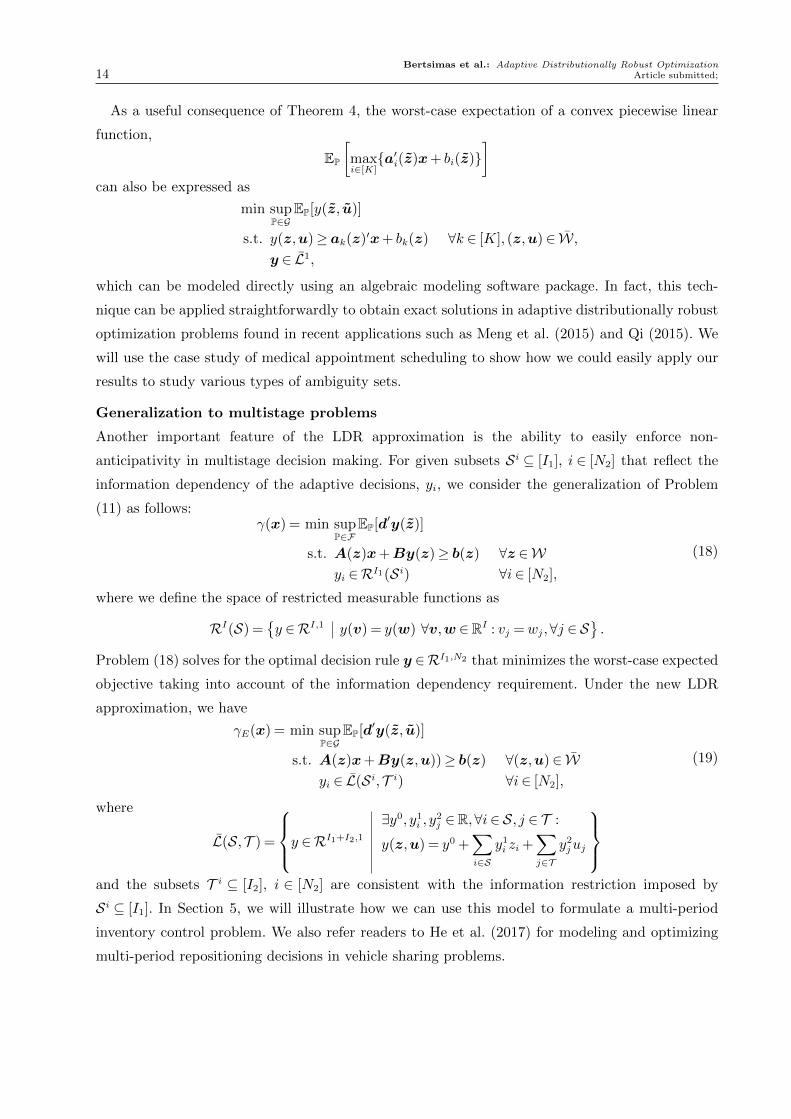
As a useful consequence of Theorem 4, the worst-case expectation of a convex piecewise linear
function,
EP
[maxi∈[K]{a′i(z)x+ bi(z)}
]can also be expressed as
min supP∈G
EP[y(z, u)]
s.t. y(z,u)≥ ak(z)′x+ bk(z) ∀k ∈ [K], (z,u)∈ W,
y ∈ L1,
which can be modeled directly using an algebraic modeling software package. In fact, this tech-
nique can be applied straightforwardly to obtain exact solutions in adaptive distributionally robust
optimization problems found in recent applications such as Meng et al. (2015) and Qi (2015). We
will use the case study of medical appointment scheduling to show how we could easily apply our
results to study various types of ambiguity sets.
Generalization to multistage problems
Another important feature of the LDR approximation is the ability to easily enforce non-
anticipativity in multistage decision making. For given subsets Si ⊆ [I1], i ∈ [N2] that reflect the
information dependency of the adaptive decisions, yi, we consider the generalization of Problem
(11) as follows:γ(x) = min sup
P∈FEP[d′y(z)]
s.t. A(z)x+By(z)≥ b(z) ∀z ∈Wyi ∈RI1(Si) ∀i∈ [N2],
(18)
where we define the space of restricted measurable functions as
RI(S) ={y ∈RI,1 y(v) = y(w) ∀v,w ∈RI : vj =wj,∀j ∈ S
}.
Problem (18) solves for the optimal decision rule y ∈RI1,N2 that minimizes the worst-case expected
objective taking into account of the information dependency requirement. Under the new LDR
approximation, we have
γE(x) = min supP∈G
EP[d′y(z, u)]
s.t. A(z)x+By(z,u))≥ b(z) ∀(z,u)∈ Wyi ∈ L(Si,T i) ∀i∈ [N2],
(19)
where
L(S,T ) =
y ∈RI1+I2,1
∃y0, y1i , y
2j ∈R,∀i∈ S, j ∈ T :
y(z,u) = y0 +∑i∈S
y1i zi +
∑j∈T
y2juj
and the subsets T i ⊆ [I2], i ∈ [N2] are consistent with the information restriction imposed by
Si ⊆ [I1]. In Section 5, we will illustrate how we can use this model to formulate a multi-period
inventory control problem. We also refer readers to He et al. (2017) for modeling and optimizing
multi-period repositioning decisions in vehicle sharing problems.
Bertsimas et al.: Adaptive Distributionally Robust OptimizationArticle submitted; 15
Enhancements of LDR approximations
As further enhancement to the LDR approximation, we can incorporate the auxiliary variables
associated with the support set as proposed in Chen et al. (2008), Chen and Zhang (2009), Goh
and Sim (2010). However, these approaches do not provide systematic ways of refining the approxi-
mations towards optimality. More recently, Zhen et al. (2016) demonstrate how an adaptive robust
or distributionally robust optimization problem can be transformed to a static robust optimiza-
tion problems via Fourier-Motzkin elimination (FME). For instance, without imposing complete
recourse, if N2 = 1, we can eliminate the only recourse variable via FME, and solve the static robust
optimization problem to optimality in polynomial time. Although this approach would generally
create exponential number of constraints, to keep the model tractable, we can perform partial FME
and apply our LDR approximation to improve the solutions. Hence, this generic reformulation tech-
nique enhances our LDR approximation and enables us to solve adaptive distributionally robust
optimization problems to the level of optimality within the limits of the available computational
resources.
On interpreting decision rule as policy and the issue of time consistency
For a given x ∈X, let y∗ be the optimal decision rule of Problem (11), and y∗E be the optimal
decision rule of Problem (15). Consider a policy based on the decision rule, y† ∈RI1,N2 such that
y†(z) = y∗E(z,g(z)).
Observe that y†(z) is feasible in Problem (11) and from the proof of Theorem 2, it follows that
β(x)≤ supP∈F
EP[d′y†(z)]≤ βE(x).
Suppose β(x) = βE(x), which is the case for complete recourse problems and N2 = 1, there is a
tendency to infer the optimality of y† vis-a-vis y∗ so that
d′y†(z) = d′y∗(z) ∀z ∈W.
However, this is not the case and we will demonstrate this fallacy in the following simple example.
Consider the following complete recourse problem,
β = min supP∈F
EP[y(z)]
s.t. y(z)≥ z ∀z ∈Ry(z)≥−z ∀z ∈Ry ∈R1,1,
(20)
where
F ={P∈P0(R) z ∼ P, EP[z] = 0,EP[z2]≤ 1
}.
Bertsimas et al.: Adaptive Distributionally Robust Optimization16 Article submitted;
Clearly, y∗(z) = |z| is the optimal solution and it is also the optimal objective value for all z ∈R.
However, under the LDR approximation, we obtain y†(z) = 1+z2
2, which is essentially greater than
the optimum policy y∗(z) except at z = 1 and z = −1. Incidentally, the worst-case distribution
P ∈ F corresponds to the two point distributions with P[z = 1] = P[z =−1] = 1/2, which explains
why their worse-case expectations coincide. This is similar to Delage and Iancu (2015) observation
that the worst-case policy generated by decision rule can be inefficient and such degeneracy is
common in robust multistage decision models.
Another issue with using the optimal decision rule as a policy is the potential violation of
time consistency. In dynamic decision making, time inconsistency arises when an optimal policy
perceived in one time period may not be recognized as optimal in another. Delage and Iancu
(2015), Xin et al. (2015) show that in addressing multiperiod robust or distributionally robust
optimization problems, time consistency may be affected by how the ambiguity sets are being
updated dynamically. While time consistency is a desirable feature in rational decision making,
policies that may violate time consistency have also been justified in the literature (see, for instance,
Basak and Chabakauri 2010, Kydland and Prescott 1977, Richardson 1989, Bajeux-Besnainou and
Portait 1998).
Consequently, when solving the adaptive distributionally robust optimization problem, we cau-
tion against using the optimal decision rule as a policy. In many practical applications of dynamic
decision making, it suffices to implement the here-and-now decision without having to commit to a
policy that dictates how the solution might change as uncertainty unfolds. For a two-stage problem,
the second stage decision should be determined by solving a linear optimization problem after the
uncertainty is resolved. In addressing a multistage decision problem, we advocate using the LDR
approximation to obtain the here-and-now decision, x∈X, which accounts for how decisions might
adapt as uncertainty unfolds over the stages. As we proceed to the next stage, we should adopt
the folding horizon approach and solve for new here-and-now decision using the latest available
information as inputs to another adaptive distributionally robust optimization problem.
Software packages
As a proof of concept, we have develop the software package, ROC (
http://www.meilinzhang.com/software) to provide an intuitive environment for formulating
and solving our proposed adaptive distributionally robust optimization models. ROC is developed
in the C++ programming language, which is fast, highly portable and well suited for deployment
in decision support systems. A typical algebraic modeling package provides the standardized
format for declaration of decision variables, transcription of constraints and objective functions,
and interface with external solvers. ROC has additional features including declaration of uncertain
Bertsimas et al.: Adaptive Distributionally Robust OptimizationArticle submitted; 17
parameters and linear decision rules, transcriptions of ambiguity sets and automatic reformulation
of standard and distributionally robust counterparts using the techniques described in this paper.
Interestingly, XProg (http://xprog.weebly.com), a new MATLAB based algebraic modeling
package that implements our proposed framework has independently emerged. The design of
XProg is similar to ROC. Since MATLAB platform is a more user friendly environment, XProg
can be used for rapid prototyping of models, while ROC would be better suited for deployment
of the solutions. The examples in our numerical studies below can easily be implemented in both
ROC and XProg.
4. An application in medical appointment scheduling
For the first application, we consider a medical appointment scheduling problem where patients
arrive at their stipulated schedule and may have to wait in a queue to be served by a physician.
The patients’ consultation times are uncertain and their arrival schedules are determined at the
first stage, which can influence the waiting times of the patients and the overtime of the physician.
To formulate the problem, we consider N patients arriving in sequence with their indices j ∈ [N ]
and the uncertain consultation times are denoted by zj, j ∈ [N ]. We let the first stage decision
variable, xj to represent the inter-arrival time between patient j to the adjacent patient j + 1 for
j ∈ [N − 1] and xN to denote the time between the arrival of the last patient and the scheduled
completion time for the physician before overtime commences. The first patient will be scheduled
to arrive at the starting time of zero and subsequent patients i, i ∈ [N ], i≥ 2 will be scheduled to
arrive at∑
j∈[i−1] xj. Consequently, the feasible region of x is given by
X =
x∈RN+ ∑i∈[N ]
xi ≤ T
,
where T is the scheduled completion time for the physician before overtime commences.
A common decision criterion in the medical appointment schedule is to minimize the expected
total cost of patients waiting and physician overtime, where the cost of a patient waiting is normal-
ized to one per unit delay and the physician’s overtime cost is γ per unit delay. For a given arrival
schedule x ∈X, and a realization of consultation times z ∈RN+ , the total cost can be determined
by solving the following linear optimization problem
Q(x,z) = min∑i∈[N ]
yi + γyN+1
s.t. yi− yi−1 +xi−1 ≥ zi−1 ∀i∈ {2, . . . ,N + 1}y≥ 0
(21)
Bertsimas et al.: Adaptive Distributionally Robust Optimization18 Article submitted;
where yi denotes the waiting time of patient i, i ∈ [N ] and yN+1 represents the overtime of the
physician. Note that the appointment scheduling problem is one that has complete recourse. From
Theorem 1, we can compute the worst-case expectation over an ambiguity set F ,
minx∈X
supP∈F
EP [Q(x, z)] ,
by enumerating all the extreme points of the corresponding dual feasible set,
P =
{p∈RN+
pi− pi−1 ≥−1 ∀i∈ {2, . . . ,N}pN ≤ γ
}.
However, given the exponentially large number of extreme points of P, it would be generally
intractable to obtain exact solutions.
Kong et al. (2013) is first to propose a distributional robust optimization for the appointment
scheduling problem. They consider a cross moment ambiguity set that characterizes the distribu-
tions of all nonnegative random variables with some specified mean values, µ and covariance Σ as
follows:
FCM =
P∈P0(RN)
z ∼ PEP[z] =µ
EP [(z−µ)(z−µ)′] = Σ
P[z ∈RN+ ] = 1
. (22)
As the problem is intractable, they formulate a SDP relaxation that solves the problem approxi-
mately.
To obtain a tractable formulation, Mak et al. (2014) ignore information on covariance and con-
sider a marginal moment ambiguity set as follows:
FMM =
P∈P0(RN)
z ∼ PEP[z] =µ
EP[(zi−µi)2] = σ2i ∀i∈ [N ]
P[z ∈RN+ ] = 1
, (23)
where σ2i , i ∈ [N ] is the variance of zi. Surprsingly, Mak et al. (2014) show that the model has
a hidden tractable reformulation, which they have cleverly exploited to obtain exact solutions.
Observe that due to equality constraints on variances, FMM is not a SOC ambiguity set. Never-
theless, by relaxing the equality constraints to inequality constraints, we will obtain the following
SOC ambiguity set:
FMM =
P∈P0(RN)
z ∼ PEP[z] =µ
EP [(zi−µi)2]≤ σ2i ∀i∈ [N ]
P[z ∈RN+ ] = 1
. (24)
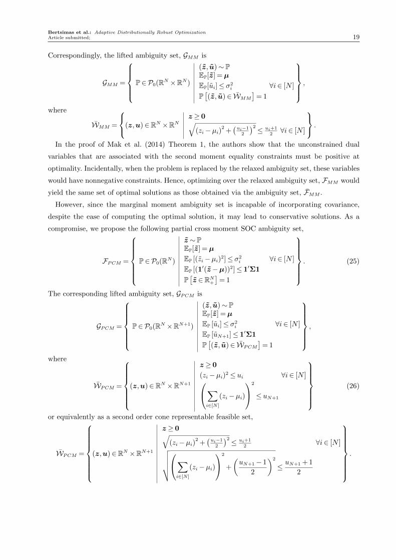
Bertsimas et al.: Adaptive Distributionally Robust OptimizationArticle submitted; 19
Correspondingly, the lifted ambiguity set, GMM is
GMM =
P∈P0(RN ×RN)
(z, u)∼ PEP[z] =µ
EP[ui]≤ σ2i ∀i∈ [N ]
P[(z, u)∈ WMM
]= 1
,
where
WMM =
(z,u)∈RN ×RNz ≥ 0√
(zi−µi)2+(ui−1
2
)2 ≤ ui+12∀i∈ [N ]
.
In the proof of Mak et al. (2014) Theorem 1, the authors show that the unconstrained dual
variables that are associated with the second moment equality constraints must be positive at
optimality. Incidentally, when the problem is replaced by the relaxed ambiguity set, these variables
would have nonnegative constraints. Hence, optimizing over the relaxed ambiguity set, FMM would
yield the same set of optimal solutions as those obtained via the ambiguity set, FMM .
However, since the marginal moment ambiguity set is incapable of incorporating covariance,
despite the ease of computing the optimal solution, it may lead to conservative solutions. As a
compromise, we propose the following partial cross moment SOC ambiguity set,
FPCM =
P∈P0(RN)
z ∼ PEP[z] =µ
EP [(zi−µi)2]≤ σ2i ∀i∈ [N ]
EP [(1′(z−µ))2]≤ 1′Σ1
P[z ∈RN+
]= 1
. (25)
The corresponding lifted ambiguity set, GPCM is
GPCM =
P∈P0(RN ×RN+1)
(z, u)∼ PEP[z] =µ
EP [ui]≤ σ2i ∀i∈ [N ]
EP [uN+1]≤ 1′Σ1
P[(z, u)∈ WPCM
]= 1
,
where
WPCM =
(z,u)∈RN ×RN+1
z ≥ 0
(zi−µi)2 ≤ ui ∀i∈ [N ]∑i∈[N ]
(zi−µi)
2
≤ uN+1
(26)
or equivalently as a second order cone representable feasible set,
WPCM =
(z,u)∈RN ×RN+1
z ≥ 0√(zi−µi)2
+(ui−1
2
)2 ≤ ui+12
∀i∈ [N ]√√√√√∑i∈[N ]
(zi−µi)
2
+
(uN+1− 1
2
)2
≤ uN+1 + 1
2
.
Bertsimas et al.: Adaptive Distributionally Robust Optimization20 Article submitted;
For these SOC ambiguity sets, we can obtain approximate solutions to the appointment schedul-
ing problem based on the new LDR approximation as follows,
min supP∈G
EP
∑i∈[N ]
yi(z, u) + γyN+1(z, u)
s.t. yi(z,u)− yi−1(z,u) +xi−1 ≥ zi−1 ∀(z,u)∈ W,∀i∈ {2, . . . ,N + 1}
y(z,u)≥ 0 ∀(z,u)∈ Wx∈Xy ∈ LN+1.
(27)
In our numerical study, we investigate the performance of appointment scheduling problem
among the following approaches,
• (Regular LDR): Solutions based on the regular LDR approximation. Note that regardless
of whether partial cross moments or marginal moments are used to define the ambiguity set, the
reformulation under the regular LDR is the same as one with an ambiguity set that has only
information on the mean and support of the random variable.
• (Exact MM): Exact solutions (Mak et al. 2014) under the marginal moment ambiguity set,
FMM .
• (Approx MM): Solutions based on the new LDR approximation under the relaxed marginal
moment ambiguity set, FMM .
• (Approx PCM): Solutions based on the new LDR approximation under the partial cross
moment ambiguity set, FPCM .
• (Approx CM): Solutions based on Kong et al. (2013) conservative SDP approximation of the
cross moment ambiguity set, FCM . Due to the instability of these models, we use three different
SDP solvers, namely SDPT3 (Tutuncu et al. 2003), SeDuMi (Strum 1999) and MOSEK, and
report only the results with confirmed status of optimality by at least one of the solvers.
The numerical settings of our computational experiments are similar to Mak et al. (2014). We
first consider N = 8 patients. The unit overtime cost is γ = 2. For each patient i∈ [N ], we randomly
select µi based on uniform distribution over [30,60] and σi = µi · ε where ε is randomly selected
based on uniform distribution over [0,0.3]. The covariance matrix is given by
[Σ]ij =
{ασiσj if i 6= jσ2j otherwise.
where α∈ [0,1] is the correlation coefficient between any two different random consultation times.
The evaluation period, T depends on the instance parameters as follows,
T =N∑i=1
µi + 0.5
√√√√ N∑i=1
σi2.
Bertsimas et al.: Adaptive Distributionally Robust OptimizationArticle submitted; 21
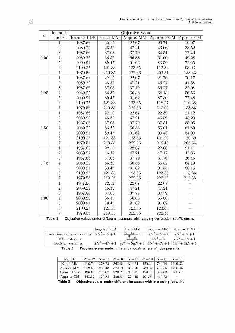
For each approach and α ∈ {0.00,0.25,0.50,0.75,1.00}, we obtain the objective values of seven
randomly generated instances. We report the results in Table 1.
Observe that Regular LDR performs extremely poorly. Indeed, as noted in Model (12), the
regular LDR approximation is unable to incorporate most of the information of the ambiguity set
other than the mean, µ and the nonnegative support set, which leads to the ultra-conservative
result. We note that Exact MM improves marginally over Approx MM, and Approx PCM improves
over Approx MM. For uncorrelated or mildly correlated random variables, i.e., α∈ {0,0.25}, Approx
PCM would yield a lower objective then. Under perfect correlation, i.e., α= 1, the objective values
of Approx PCM and Approx MM coincide and they are marginally higher than the objective
values of Exact MM. Hence, while there are benefits from the new LDR approximation, it does
not replicate the optimal solution of Mak et al. (2014).
In Table 2, we show how the size of the four tractable models (Regular LDR, Exact MM, Approx
MM and Approx PCM) scales with the number of jobs, N . For Approx CM, unlike the previous
approaches, we are unable to obtain its optimally verified solutions by all the three SDP solvers
when the correlation is high. Among the instances that the solutions of Approx CM could be
optimally verified by at least one of the solvers, we observe that the corresponding objective values
attained are the lowest values among the approaches.
In Table 3 and Table 4, we increase the number of jobs from N = 12 to N = 30 and report the
objective values and computational times for the different approaches. In this numerical study, we
set α= 0 and ε= 0.15. The results indicate that the approach with a tighter approximation also
incurs a longer computational time. Observe that it takes significantly longer time to solve Approx
CM and more seriously, its solution may not necessarily be optimally verified by the SDP solvers
as the problem size increases. In contrast, the Approx PCM can be computed quickly and reliably
and its solution consistently improves over Exact MM and Approx MM for the case when α= 0.
Hence, this underscores the importance of having a stable optimization format and reaffirm our
restriction to SOC ambiguity set.
Similar to Mak et al. (2014), we also compare the performance of the approaches in out-of-
sample study using truncated normal and log normal probability distributions. We assume that
the underlying random variables are independently distributed and the parameters of the distri-
butions correspond to the respective ambiguity sets for which the distributionally robust solutions
are obtained. Upon obtaining the solutions from the various methods, we compare the perfor-
mance and present the results in Table 5. These values are evaluated via Monte Carlo simulation
with 10,000 trials under each specific distribution. Interestingly, despite the differences in objec-
tive values attained, the out-of-sample study alludes to the closeness of results between Exact
Bertsimas et al.: Adaptive Distributionally Robust Optimization22 Article submitted;
αInstance Objective Value
Index Regular LDR Exact MM Approx MM Approx PCM Approx CM
0.00
1 1987.66 22.12 22.67 20.71 19.272 2089.22 46.32 47.21 43.06 33.523 1987.66 37.03 37.79 34.51 27.404 2089.22 66.32 66.88 61.00 49.285 2009.91 89.47 91.62 83.59 72.256 2100.27 121.33 123.65 112.33 93.237 1979.56 219.35 222.36 202.51 158.43
0.25
1 1987.66 22.12 22.67 21.76 20.172 2089.22 46.32 47.21 45.27 41.383 1987.66 37.03 37.79 36.27 32.084 2089.22 66.32 66.88 64.13 56.565 2009.91 89.47 91.62 87.80 77.486 2100.27 121.33 123.65 118.27 110.387 1979.56 219.35 222.36 213.09 188.86
0.50
1 1987.66 22.12 22.67 22.39 21.122 2089.22 46.32 47.21 46.59 43.203 1987.66 37.03 37.79 37.31 35.054 2089.22 66.32 66.88 66.01 61.895 2009.91 89.47 91.62 90.43 84.906 2100.27 121.33 123.65 121.90 120.697 1979.56 219.35 222.36 219.43 206.34
0.75
1 1987.66 22.12 22.67 22.66 21.112 2089.22 46.32 47.21 47.17 43.863 1987.66 37.03 37.79 37.76 36.454 2089.22 66.32 66.88 66.82 64.195 2009.91 89.47 91.62 91.55 88.166 2100.27 121.33 123.65 123.53 115.367 1979.56 219.35 222.36 222.18 213.55
1.00
1 1987.66 22.12 22.67 22.67 –2 2089.22 46.32 47.21 47.21 –3 1987.66 37.03 37.79 37.79 –4 2089.22 66.32 66.88 66.88 –5 2009.91 89.47 91.62 91.62 –6 2100.27 121.33 123.65 123.65 –7 1979.56 219.35 222.36 222.36 –
Table 1 Objective values under different instances with varying correlation coefficient α.
Regular LDR Exact MM Approx MM Approx PCM
Linear inequality constraints 2N2 +N + 1 (N+1)N2
+ 1 2N2 +N + 1 2N2 +N + 1
SOC constraints 0 (N+1)N2
2N2 +N 2N2 + 3N + 1Decision variables 2N2 + 4N + 1 1
2N2 + 5 1
2N + 1 6N2 + 8N + 1 6N2 + 12N + 5
Table 2 Problem scales under different models where N jobs presents.
Models N = 12 N = 14 N = 16 N = 18 N = 20 N = 25 N = 30
Exact MM 216.74 278.75 368.62 364.84 520.24 736.24 1129.32Approx MM 219.65 288.48 374.71 380.50 538.52 796.55 1206.43Approx PCM 196.64 255.07 329.23 333.67 459.48 608.02 889.51Approx CM 143.87 179.88 226.84 224.29 301.04 419.72 –
Table 3 Objective values under different instances with increasing jobs, N .

Bertsimas et al.: Adaptive Distributionally Robust OptimizationArticle submitted; 23
Models N = 12 N = 14 N = 16 N = 18 N = 20 N = 25 N = 30
Exact MM < 1 < 1 < 1 < 1 < 1 < 1 < 1Approx MM < 1 < 1 < 1 < 1 < 1 < 1 1Approx PCM < 1 < 1 < 1 < 1 < 1 < 1 2Approx CM 7 15 31 57 123 378 –
Table 4 Computation time under different instances with increasing jobs, N .
MM and Approx MM as well as between Approx PCM and Approx CM. Since the random vari-
ables are independent, and hence uncorrelated, as we have expected, incorporating covariance or
partial covariance information in the ambiguity would lead to improvement in the out-of-sample
performances.
Instance Models Objective Truncated LogIndex Value Normal Normal
1
Regular LDR 1987.66 1306.37(0.58) 1306.36(0.61)Exact MM 22.12 11.12(0.25) 11.07(0.3)
Approx MM 22.67 11.08(0.30) 11.16(0.31)Approx PCM 20.71 10.99(0.26) 10.10(0.27)Approx CM 19.27 10.68(0.25) 10.07(0.26)
2
Regular LDR 2089.22 1328.41(1.20) 1328.40(1.17)Exact MM 46.32 22.17(0.50) 22.12(0.51)
Approx MM 47.21 22.27(0.51) 22.48(0.52)Approx PCM 43.06 22.09(0.49) 20.19(0.51)Approx CM 33.52 22.12(0.51) 19.86(0.52)
3
Regular LDR 1987.66 1307.89(0.96) 1307.88(1.01)Exact MM 37.03 18.75(0.41) 18.25(0.42)
Approx MM 37.79 18.47(0.40) 18.65(0.41)Approx PCM 34.51 16.72(0.41) 16.90(0.42)Approx CM 27.40 16.67(0.40) 16.76(0.41)
4
Regular LDR 2089.22 1329.58(1.70) 1329.54(1.68)Exact MM 66.32 31.13(0.76) 31.36(0.78)
Approx MM 66.88 31.55(0.73) 31.96(0.76)Approx PCM 61.00 28.32(0.74) 28.70(0.78)Approx CM 49.28 28.20(0.76) 28.60(0.78)
5
Regular LDR 2009.91 1323.02(2.52) 1323.23(2.56)Exact MM 89.47 42.08(0.96) 43.93(1.03)
Approx MM 91.62 43.10(0.93) 44.09(0.99)Approx PCM 83.59 39.32(0.97) 40.26(1.05)Approx CM 72.25 38.94(0.98) 39.15(1.03)
6
Regular LDR 2100.27 1357.65(3.03) 1357.59(3.15)Exact MM 121.33 55.69(1.23) 56.15(1.28)
Approx MM 123.65 56.45(1.19) 57.75(1.25)Approx PCM 112.33 50.66(1.18) 51.87(1.32)Approx CM 88.42 48.23(1.22) 51.07(1.31)
7
Regular LDR 1979.56 1271.30(5.87) 1272.27(6.13)Exact MM 219.35 103.36(2.51) 107.89(3.05)
Approx MM 222.36 105.61(2.49) 109.97(2.98)Approx PCM 202.51 96.49(2.52) 100.54(3.11)Approx CM 156.15 95.46(2.50) 99.26(3.14)
Table 5 Results of Monte Carlo simulation under truncated normal and log normal distributions.
Asterisks indicate suboptimal solutions and standard errors are reported in parenthesis .
Bertsimas et al.: Adaptive Distributionally Robust Optimization24 Article submitted;
5. An application in multi-period inventory control
For the second application, we illustrate how the adaptive distributionally robust linear optimiza-
tion framework can model a multistage decision problem. We consider a finite horizon, T period
single product inventory control problem. Demands are filled from on-hand inventory and unfilled
demands are fully backlogged. At the beginning of period t, a quantity of xt ∈ [0, xt] is ordered,
which will arrive immediately to replenish the stock before the demand is realized. The unit order-
ing cost is ct, excess inventory will incur a per-unit holding cost of ht, while backlogged demand
will be penalized with a per-unit underage cost of bt. At the last period t= T , lost sales could be
accounted for via the backorder cost. We use yt to indicate the net inventory level at the beginning
of period t. The initial net inventory level of the system is y1 = 0.
As in Graves (1999) and See and Sim (2009), we model the demand process is an integrated
moving average (IMA) process of order (0,1,1) as follows:
dt(z) = zt +αzt−1 +αzt−2 + · · ·+αz1 +µ= dt−1(z)− (1−α)zt−1 + zt,
for t ∈ [T ], where α ∈ [0,1] and the uncertain factors, zt are zero means and uncorrelated ran-
dom variables. Hence, with α= 0, the demands are uncorrelated. As α grows, the variances and
correlation of the demands also increase.
The objective of the problem is to minimize the worst-case expected total cost over the entire
horizon as follows,
min supP∈F
EP
[T∑t=1
(ctxt(zt−1) + vt(zt))
]s.t. yt+1(zt) = yt(zt−1) +xt(zt−1)− dt(zt) ∀z ∈W, t∈ [T ]
vt(zt)≥ htyt+1(zt) ∀z ∈W, t∈ [T ]
vt(zt)≥−btyt+1(zt) ∀z ∈W, t∈ [T ]
0≤ xt(zt−1)≤ xt ∀z ∈W, t∈ [T ]
xt ∈Rt−1,1, yt+1 ∈Rt,1, vt ∈Rt,1 ∀t∈ [T ].
(28)
We consider the following partial cross moment ambiguity set,
FPCM =
P∈P0(RT )
z ∼ PEP[z] = 0
EP
( t∑r=s
zr
)2≤ φ2
st ∀s≤ t, s, t∈ [T ]
P [z ∈ [z, z]] = 1
, (29)
where the lifted ambiguity set, G is
GPCM =
P∈P0(RT ×R(T+1)T/2)
(z, u)∼ PEP[z] = 0
EP[ust]≤ φ2st ∀s≤ t, s, t∈ [T ]
P[(z, u)∈ WPCM
]= 1
, (30)
Bertsimas et al.: Adaptive Distributionally Robust OptimizationArticle submitted; 25
WPCM =
(z,u)∈RT ×R(T+1)T/2 ust ≥
(t∑
r=s
zr
)2
∀s≤ t, s, t∈ [T ]
z ∈ [z, z]
.
This partial cross moment incorporates the variances of the sum of factors leading to the time period
t. We let ut = (urs)1≤r≤s≤t, t ∈ [T ], which, together with zt are associated with the information
available at the end of period t. Consequently, we use ROC to formulate the problem via the new
LDR approximation and solve it using CPLEX.
Following the numerical study of See and Sim (2009), we set the parameters xt = 260, ct = 0.1,
ht = 0.02, for all t ∈ [T ], bt = 0.2, for all t ∈ [T − 1] and bT = 2. We assume that random factors zt
are uncorrected random variables in [−z, z] with standard deviations bounded below by 1√3z. In
characterizing the partial cross moment ambiguity set, we have µt = µ, t∈ [T ] and
φ2st =
(t− s+ 1)
3z2 ∀s≤ t, s, t∈ [T ].
Observe that iid uniformly distributed random variables in [−z, z] would be a feasible distribution
in the ambiguity set and we use this to obtain a lower bound to the inventory control problem.
Specifically, we investigate the performance of the multi-period inventory control problem among
different approaches as follows,
• (Lower Bound): A lower bound obtained by using iid uniformly distributed random factors
and solving the dynamic inventory control problem to optimality (for the dynamic programming
implementation, see See and Sim 2009).
• (Approx MM): Solutions based on the new LDR approximation under the marginal moment
ambiguity set (i.e. known mean values, upper bound on variances and nonnegative support).
• (Approx PCM): Solutions based on the new LDR approximation under the partial cross
moment ambiguity set, FPCM .
In Table 6, we report the objective values attained for the different approaches under various
parameters. As in the previous computational study, we observe that by incorporating partial cross
moment information, we can significantly improve the objectives of the adaptive distributionally
robust optimization problems. Moreover, the objectives of Approx PCM are reasonably close to
the lower bounds. It has well been known that despite the gaps from the lower bounds, numerical
experiments on robust inventory control problems have demonstrated that the actual objectives
attained in out-of-sample analysis are often closer to the optimal values than what the model objec-
tives have reflected (see, for instance, Bertsimas and Thiele 2006, See and Sim 2009). Moreover,
the benefit of distributional robustness arises when there is disparity between the actual demand
distribution and the demand distribution in which the optimal policy is derived. In such cases,
the robust solution could perform significantly better than the misspecified optimum policy (see,
numerical experiments of Bertsimas and Thiele 2006).

Bertsimas et al.: Adaptive Distributionally Robust Optimization26 Article submitted;
T µ z α Lower Approx MM Approx PCMBound
5 200 20 0 108.0 167.3 115.710 200 10 0 206.0 272.5 214.920 240 6 0 486.0 583.2 499.230 240 4 0 725.0 838.6 740.8
5 200 20 0.25 108.0 181.0 124.810 200 10 0.25 206.0 303.7 232.820 240 6 0.25 487.0 684.7 543.630 240 4 0.25 725.0 1028.8 811.2
5 200 20 0.50 109.0 195.1 133.610 200 10 0.50 207.0 335.2 250.720 240 6 0.50 496.0 795.1 588.430 240 4 0.50 732.0 1232.2 882.9
Table 6 Objective values of the various models under different instances.
6. Future work
In our numerical studies, we show the benefits of the partial cross moments ambiguity set. However,
the choice of such ambiguity set appears ad hoc and it begs an interesting question as to how we
can systematically adapt and improve the partial cross moments ambiguity set. Chen et al. (2016)
have recently proposed a new class of infinitely constrained ambiguity sets where the number of
expectation constraints could be infinite. To solve the problem, they consider a relaxed ambiguity
set with finite number of expectation constraints, as in the case of the partial cross moments ambi-
guity set. More interestingly, for static robust optimization problems, the “violating” expectation
constraint can be identified and added to the relaxed ambiguity set to improve the solution. While
the approach works for static distributionally robust optimization problems, the extension to adap-
tive problems has not been studied. We believe this is an important extension of this framework
that will help us model and solve adaptive distributionally robust optimization problems for a
larger variety of ambiguity sets.
Acknowledgments
The authors would like to thank the Department Editor, Professor Noah Gans, the anonymous AE and the
reviewers for their valuable and insightful comments. The research is funded by NUS Global Asia Institute
and the Singapore Ministry of Education Social Science Research Thematic Grant MOE2016-SSRTG-059.
Any opinions, findings, and conclusions or recommendations expressed in this material are those of the
authors and do not reflect the views of the Singapore Ministry of Education or the Singapore Government.
References
Alizadeh, F., D. Goldfarb (2003) Second-order cone programming. Math. Programming 95(1):2–51.
Bajeux-Besnainou, Isabelle, Roland Portait (1998) Dynamic asset allocation in a mean-variance framework.
Management Science 44.11-part-2 (1998): S79-S95.
Bertsimas et al.: Adaptive Distributionally Robust OptimizationArticle submitted; 27
Basak, Suleyman, Georgy Chabakauri (2010) Dynamic mean-variance asset allocation. Review of financial
Studies 23(8): 2970–3016.
Ben-Tal, A., den Hertog, D. and Vial, J. (2015) Deriving robust counterparts of nonlinear uncertain inequal-
ities. Math. Programming 149(1):265–299.
Ben-Tal, A., A. Nemirovski (1998) Robust convex optimization. Math. Oper. Res. 23(4):769–805.
Ben-Tal, A., A. Nemirovski (1999) Robust solutions of uncertain linear programs. Oper. Res. Lett 25(1,
Auguest):1–13.
Ben-Tal, A., A. Nemirovski (2000) Robust solutions of linear programming problems contaminated with
uncertain data. Math. Programming Ser. A 88(3):411–424.
Ben-Tal, A., A. Nemirovski (2001a) Lectures on Modern Convex Optimization: Analysis, Algorithms, and
Engineering Applications. SIAM.
Ben-Tal, A., A. Nemirovski (2001b) On polyhedral approximations of the second-order cone Mathematics of
Operations Research 26:193–205
Ben-Tal, A., A. Goryashko, E.Guslitzer, A. Nemirovski (2004) Adjustable robust solutions of uncertain linear
programs. Math. Programming 99:351-376.
Bertsimas, D., D. A. Iancu, P. A. Parrilo (2010) Optimality of Affine Policies in Multistage Robust Opti-
mization. Mathematics of Operations Research 35(2):363–394.
Bertsimas, D., D.B. Brown (2009) Constructing uncertainty sets for robust linear optimization. Operations
Research 57(6) 1483-1495.
Bertsimas, D., Brown, D. B., Caramanis, C. (2011). Theory and applications of robust optimization. SIAM
review, 53(3), 464-501.
Bertsimas, D., Popescu, I. (2005) Optimal inequalities in probability theory: A convex optimization approach.
SIAM Journal on Optimization 15(3):780-804.
Bertsimas, D., M. Sim (2004) The price of robustness. Oper. Res. 52(1):35–53.
Bertsimas, D., A. Thiele (2006) A robust optimization approach to inventory theory. Oper. Res. 54(1):150–
168.
Birge, J. R., F. Louveaux (1997) Introduction to Stochastic Programming. Springer, New York.
Breton, M., S. El Hachem (1995) Algorithms for the solution of stochastic dynamic minimax problems.
Comput. Optim. Appl. 4:317–345.
Chen, W., M. Sim (2009) Goal-driven optimization. Operations Research 57(2)(2):342–357.
Chen, Z., M. Sim., H. Xu (2016) Distributionally Robust Optimization with Infinitely Constrained Ambiguity
Sets Optimization online
Chen, X., Y. Zhang (2009) Uncertain linear programs: Extended affinely adjustable robust counterparts.
Oper. Res. 57(6):1469–1482.
Bertsimas et al.: Adaptive Distributionally Robust Optimization28 Article submitted;
Chen, X., M. Sim, P. Sun (2007) A robust optimization perspective on stochastic programming. Operations
Research, 55(6):1058–1071.
Chen, X., M. Sim, P. Sun, J. Zhang (2008) A linear decision-based approximation approach to stochastic
programming. Oper. Res. 56(2):344–357.
Delage, E., Dan Iancu (2015) Robust multi-stage decision making. INFORMS Tutorials in Operations
Research (2015): 20–46.
Delage, E., Y. Ye (2010) Distributionally robust optimization under moment uncertainty with application
to data-driven problems. Oper. Res. 58(3):596–612.
Dupacova, J.(1987) The minimax approach to stochastic programming and an illustrative application.
Stochastics 20(1):73–88.
Dyer, M., L. Stougie (2006) Computational complexity of stochastic programming problems. Math. Pro-
gramming Ser. A 106:423–432.
Ellsberg, D. (1961) Risk, ambiguity and the Savage axioms. Quarterly Journal of Economics, 75(4), pp.
643-669.
Garstka, S. J., R. J.-B. Wets (1974) On decision rules in stochastic programming. Math. Programming
7(1):117-143.
Ghaoui, El. L., H. Lebret (1997) Robust solutions to least-squares problems with uncertain data. SIAM
J.Matrix Anal. Appl.18(4):1035–1064.
Ghaoui, El. L., F. Oustry, H. Lebret (1998) Robust solutions to uncertain semidefinite programs. SIAM J.
Optim. 9:33–53.
Gilboa, I., D. Schmeidler (1989) Maxmin expected utility with non-unique prior. Journal of Mathematical
Economics 18(2):141–153.
Goh, J., M. Sim (2009) Robust optimization made easy with ROME. Oper. Res. 59(4):973–985.
Goh, J., M. Sim (2010) Distributionally robust optimization and its tractable approximations. Oper. Res.
58(4):902–917.
Graves, S. C. (1999) A single-item inventory model for a nonstationary demand process. Manufacturing &
Service Operations Management 1(1):50–61.
He, Long, Zhenyu Hu, Meilin Zhang (2017) Robust Repositioning for Vehicle Sharing. NUS Working paper
Hsu M., M. Bhatt, R. Adolphs, D. Tranel, C.F. Camerer. (2005). Neural systems responding to degrees of
uncertainty in human decision-making. Science 310 1680–1683.
Isii, K. (1962) On sharpness of tchebycheff-type inequalities. Annals of the Institute of Statistical Mathematics
14(1):185–197.
Knight, F. H. (1921) Risk, uncertainty and profit. Hart, Schaffner and Marx.
Bertsimas et al.: Adaptive Distributionally Robust OptimizationArticle submitted; 29
Kong, Q., Lee, C. Y., Teo, C. P., Zheng, Z. (2013). Scheduling arrivals to a stochastic service delivery system
using copositive cones. Oper. Res. 61(3): 711726.
Kuhn, D., W. Wiesemann, A. Georghiou (2011) Primal and dual linear decision rules in stochastic and robust
optimization. Math. Programming 130(1):177–209.
Kydland, Finn E., Edward C. Prescott (1977) Rules rather than discretion: The inconsistency of optimal
plans. The journal of political Economy: 473-491.
Lobo, M., L. Vandenberghe, S. Boyd, H. Lebret (1998) Applications of second-order cone programming.
Linear Algebra and its Applications 284(1-3):193–228.
Loberg, J. (2012) Automatic robust convex programming. Optimization methods and software 27(1): 115–129.
Mak, H. Y., Rong, Y., Zhang, J. (2014) Appointment scheduling with limited distributional information.
Management Science 61(2): 316-334.
F. Meng, J. Qi, M. Zhang, J. Ang, S. Chu, M. Sim (2015) A robust optimization model for managing elective
admission in a public hospital. Operations Research 63(6):1452–1467.
Popescu, I. (2007) Robust mean-covariance solutions for stochastic optimization. Oper. Res. 55(4):98–112.
J. Qi (2015) Mitigating delays and unfairness in appointment systems. Management Science 63(2):566-583.
Richardson, Henry R (1989) A minimum variance result in continuous trading portfolio optimization. Man-
agement Science 35(9): 1045–1055.
Ruszczynski, A., A. Shapiro (2003) Stochastic Programming. Handbooks in Operations Research and Man-
agement Science 10. Elsevier Science, Amsterdam.
Shapiro, A., A. Kleywegt (2002) Minimax analysis of stochastic programs. Optimization Methods and Soft-
ware, 17(3):523–542.
Scarf, H. (1958) A min-max solution of an inventory problem. K. Arrow, ed. Studies in the Mathematical
Theory of Inventory and Production. Stanford University Press, Stanford, CA, 201–209.
See, C.-T., M. Sim (2009) Robust approximation of multiperiod inventory management. Oper. Res. 58(3):583–
594.
Shapiro, A., S. Ahmed (2004) On a class of minimax stochastic programs. SIAM Journal on Optimization
14(4):1237–1249.
Shapiro, A., A. Nemirovski (2005) On complexity of stochastic programming problems. V. Jeyakumar, A.
Rubinov, eds. Continuous Optimization. Springer, New York, 111–146.
Sturm, J. F. (1999) Using SeDuMi 1.02, a MATLAB toolbox for optimization over symmetric cones. Opti-
mization methods and software 11(1-4), 625–653.
Tutuncu, R.H., K.C. Toh, and M.J. Todd (2003) Solving semidefinite-quadratic-linear programs using
SDPT3. Mathematical Programming Ser. B 95:189–217.
Bertsimas et al.: Adaptive Distributionally Robust Optimization30 Article submitted;
Wiesemann, W., D. Kuhn, M. Sim (2014) Distributionally Robust Convex Optimization. Operations Research
62(6): 1358–1376.
Xin, L., DA. Goldberg, and A. Shapiro (2015) Time (in)consistency of multistage distributionally robust
inventory models with moment constraints. https://arxiv.org/abs/1304.3074.
Xu, H., S. Mannor (2012) Distributionally robust Markov decision processes. Mathematics of Operations
Research 37(2):288–300.
Zackova, J . (1966) On minimax solution of stochastic linear programming problems. Casopis pro Pestovanı
Matematiky, 91:423–430.
Zhen, J., M. Sim, den Hertog, D. (2016) Adjustable Robust Optimization via Fourier-Motzkin Elimination
Optimization online

e-companion to Bertsimas et al.: Adaptive Distributionally Robust Optimization ec1
Eletronic Companion
EC.1. Proof of Theorem 1
From Proposition 1, we have equivalently
β(x) = supP∈F
EP [Q(x, z)] = supP∈G
EP [Q(x, z)] .
For any feasible solution in (9) and (z, u)∼ P∈ G observe that
EP [Q(x, z)]≤EP [r+ s′(Gz) + t′u]≤ r+ s′µ+ t′σ.
Hence, we have
β(x)≤ β1(x) = inf r+ s′µ+ t′σ
s.t. r+ s′(Gz) + t′u≥Q(x,z) ∀(z,u)∈ Wt≥ 0
r ∈R,s∈RL1 , t∈RI2 ,
where r ∈R,s∈RL1 , t∈RI2 are the dual variables corresponding to the expectation constraints of
the ambiguity set, G.
Under the assumption of relatively complete recourse, Q(x,z) is finite and by strong duality of
linear optimization, we have equivalently
Q(x,z) = maxp∈P
p′(b(z)−A(z)x) = maxp∈[P ]
{p′p(b(z)−A(z)x)
}.
Therefore,
β1(x) = inf r+ s′µ+ t′σ
s.t. r≥ sup(z,u)∈W
p′p(b
1−A1x)
...
p′p(bI1 −AI1x)
−G′s′
z− t′u+p′p(b0−A0x)
∀p∈ [P ]
t≥ 0
r ∈R,s∈RL1 , t∈RI2 .(EC.1)
ec2 e-companion to Bertsimas et al.: Adaptive Distributionally Robust Optimization
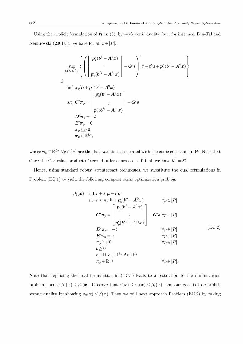
Using the explicit formulation of W in (8), by weak conic duality (see, for instance, Ben-Tal and
Nemirovski (2001a)), we have for all p∈ [P ],
sup(z,u)∈W
p′p(b
1−A1x)
...
p′p(bI1 −AI1x)
−G′s′
z− t′u+p′p(b0−A0x)
≤
inf πp′h+p′p(b
0−A0x)
s.t. C ′πp =
p′p(b
1−A1x)
...
p′p(bI1 −AI1x)
−G′sD′πp =−tE′πp = 0
πp �K 0
πp ∈RL2 ,
where πp ∈RL2 ,∀p∈ [P ] are the dual variables associated with the conic constants in W. Note that
since the Cartesian product of second-order cones are self-dual, we have K∗ =K.
Hence, using standard robust counterpart techniques, we substitute the dual formulations in
Problem (EC.1) to yield the following compact conic optimization problem
β2(x) = inf r+ s′µ+ t′σ
s.t. r≥πp′h+p′p(b0−A0x) ∀p∈ [P ]
C ′πp =
p′p(b
1−A1x)
...
p′p(bI1 −AI1x)
−G′s ∀p∈ [P ]
D′πp =−t ∀p∈ [P ]
E′πp = 0 ∀p∈ [P ]
πp �K 0 ∀p∈ [P ]
t≥ 0
r ∈R,s∈RL1 , t∈RI2πp ∈RL2 ∀p∈ [P ].
(EC.2)
Note that replacing the dual formulation in (EC.1) leads to a restriction to the minimization
problem, hence β1(x) ≤ β2(x). Observe that β(x) ≤ β1(x) ≤ β2(x), and our goal is to establish
strong duality by showing β2(x) ≤ β(x). Then we will next approach Problem (EC.2) by taking

e-companion to Bertsimas et al.: Adaptive Distributionally Robust Optimization ec3
the dual, which is
β3(x) = sup∑p∈[P ]
p′p(b0−A0x)αp +
p′p(b1−A1x)
...p′p(b
I1 −AI1x)
′
zp
s.t.
∑p∈[P ]
αp = 1
αp ≥ 0 ∀p∈ [P ]∑p∈[P ]
Gzp =µ∑p∈[P ]
up ≤σ
Czp +Dup +Evp �K αph ∀p∈ [P ]αp ∈R, zp ∈RI1 , ∀p∈ [P ]up ∈RI2 , vp ∈RI3 ∀p∈ [P ],
(EC.3)
where αp, z, up, vp,∀p∈ [P ] are the dual variables associated with the specified constraints respec-
tively. Under the Slater’s condition, there exists u† ∈RI2 and v† ∈RI3 such that
u† <σ
Cz†+Du†+Ev† ≺K h.
Therefore, we can construct a strictly feasible solution
αp =1
P, zp =
z†
P, up =
u†
P, vp =
v†
P,
for all p ∈ [P ]. Since Problem (EC.3) is strictly feasible, strong duality holds and β2(x) = β3(x).
Moreover, there exists a sequence of interior solutions
{(αkp, z
kp, u
kp, v
kp)p∈[P ]
}k≥0
such that
limk→∞
∑p∈[P ]
p′p(b0−A0x)αkp +
p′p(b1−A1x)
...p′p(b
I1 −AI1x)
′
zkp
= β3(x).
Observe that for all k, αkp > 0,∑p∈[P ]
αkp = 1 and we can construct a sequence of discrete probability
distributions {Pk ∈P0 (RI1 ×RI2)}k≥0 on random variable (z, u)∼ Pk such that
Pk[(z, u) =
(zk
p
αkp,uk
p
αkp
)]= αkp ∀p∈ [P ].
Note that,
EPk [Gz] =µ,EPk [u]≤σ,Pk[(z, u)∈ W] = 1,

ec4 e-companion to Bertsimas et al.: Adaptive Distributionally Robust Optimization
and hence Pk ∈ G for all k. Moreover,
β3(x) = limk→∞
∑p∈[P ]
p′p(b0−A0x)αkp +
p′p(b1−A1x)
...p′p(b
I1 −AI1x)
′
zkp
= lim
k→∞
∑p∈[P ]
αkp
p′p(b0−A0x) +
p′p(b1−A1x)
...p′p(b
I1 −AI1x)
′
zkpαkp
≤ lim
k→∞
∑p∈[P ]
αkp
maxq∈[P ]
p′q(b0−A0x) +
p′q(b1−A1x)
...p′q(b
I1 −AI1x)
′
zkqαkq
= limk→∞
EPk
maxq∈[P ]
p′q(b0−A0x) +
p′q(b1−A1x)
...p′q(b
I1 −AI1x)
′
z
≤ supP∈G
EP[Q(x,z)]
= β(x).
Hence, β(x)≤ β1(x)≤ β2(x) = β3(x)≤ β(x).
EC.2. Proof of Theorem 3
Let σ> 0 be such that
EP[|zi|]≤ σi ∀P∈F .
Consider the following lifted ambiguity set F is
G =
P∈P0(RI1 ×RI1)
(z, u)∼ P∏z P∈F
EP[u]≤σP[(z, u)∈ W] = 1
,
where the lifted support set is W = {(z,u) ∈RI1 ×RI1 | u≥ z,u≥−z}. The decision rule under
the new LDR approximation is given by
y(z,u) = y0 +∑i∈[I1]
y1i zi +
∑i∈[I1]
y2iui.
To show that Problem (15) is feasible and finite under the new LDR, we consider the following
relaxed lifted ambiguity set
G =
P∈P0(RI1 ×RI1)
(z, u)∼ PEP[u]≤σP[(z, u)∈ W] = 1
,
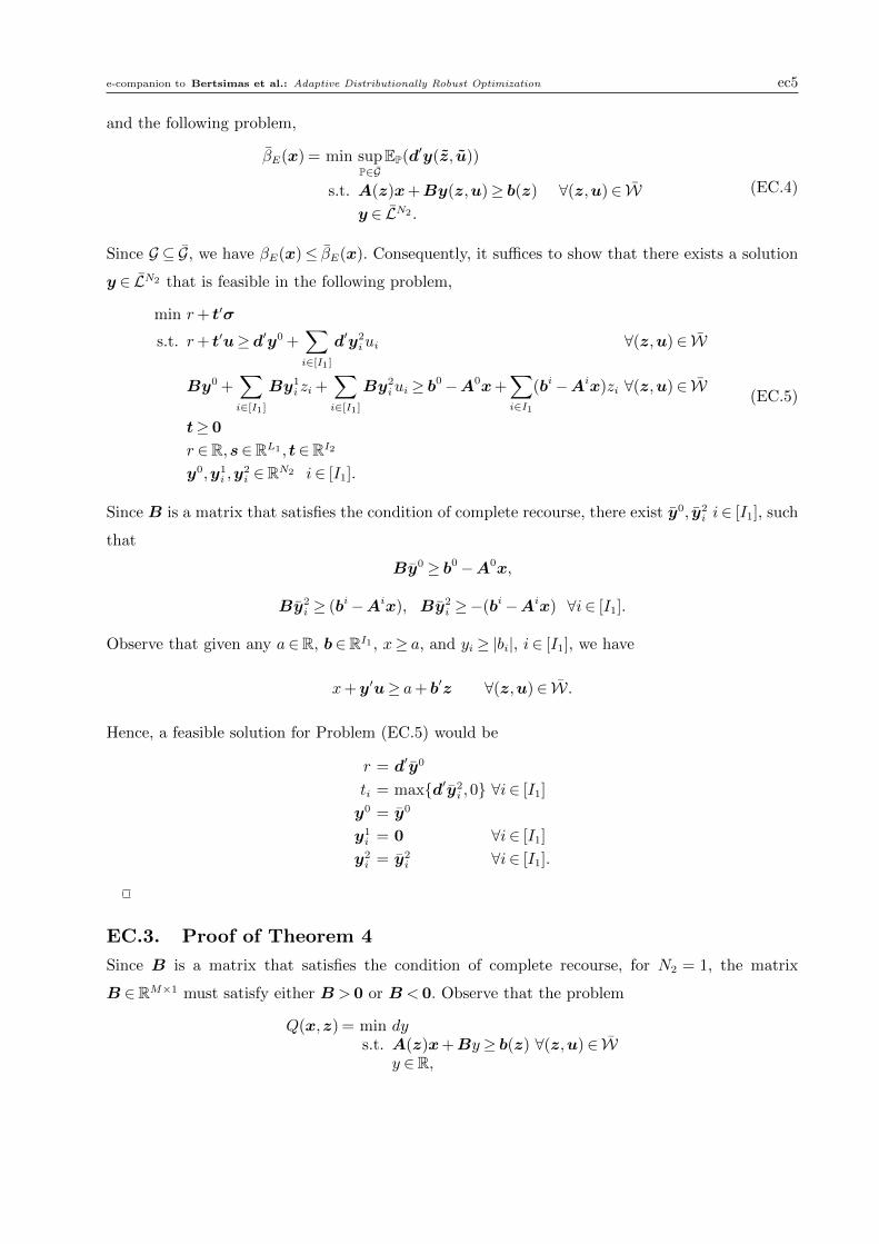
e-companion to Bertsimas et al.: Adaptive Distributionally Robust Optimization ec5
and the following problem,
βE(x) = min supP∈G
EP(d′y(z, u))
s.t. A(z)x+By(z,u)≥ b(z) ∀(z,u)∈ Wy ∈ LN2 .
(EC.4)
Since G ⊆ G, we have βE(x)≤ βE(x). Consequently, it suffices to show that there exists a solution
y ∈ LN2 that is feasible in the following problem,
min r+ t′σ
s.t. r+ t′u≥ d′y0 +∑i∈[I1]
d′y2iui ∀(z,u)∈ W
By0 +∑i∈[I1]
By1i zi +
∑i∈[I1]
By2iui ≥ b
0−A0x+∑i∈I1
(bi−Aix)zi ∀(z,u)∈ W
t≥ 0
r ∈R,s∈RL1 , t∈RI2y0,y1
i ,y2i ∈RN2 i∈ [I1].
(EC.5)
Since B is a matrix that satisfies the condition of complete recourse, there exist y0, y2i i∈ [I1], such
that
By0 ≥ b0−A0x,
By2i ≥ (bi−Aix), By2
i ≥−(bi−Aix) ∀i∈ [I1].
Observe that given any a∈R, b∈RI1 , x≥ a, and yi ≥ |bi|, i∈ [I1], we have
x+y′u≥ a+ b′z ∀(z,u)∈ W.
Hence, a feasible solution for Problem (EC.5) would be
r = d′y0
ti = max{d′y2i ,0} ∀i∈ [I1]
y0 = y0
y1i = 0 ∀i∈ [I1]
y2i = y2
i ∀i∈ [I1].
EC.3. Proof of Theorem 4
Since B is a matrix that satisfies the condition of complete recourse, for N2 = 1, the matrix
B ∈RM×1 must satisfy either B > 0 or B < 0. Observe that the problem
Q(x,z) = min dys.t. A(z)x+By≥ b(z) ∀(z,u)∈ W
y ∈R,
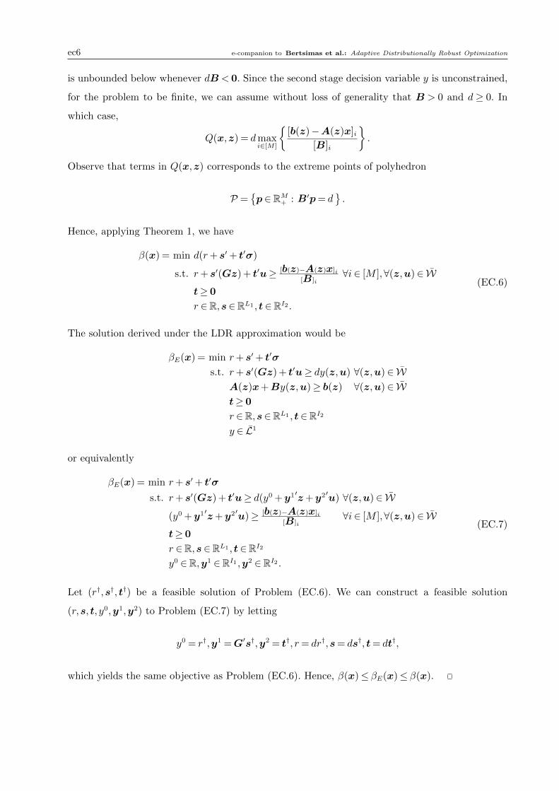
ec6 e-companion to Bertsimas et al.: Adaptive Distributionally Robust Optimization
is unbounded below whenever dB < 0. Since the second stage decision variable y is unconstrained,
for the problem to be finite, we can assume without loss of generality that B > 0 and d ≥ 0. In
which case,
Q(x,z) = dmaxi∈[M ]
{[b(z)−A(z)x]i
[B]i
}.
Observe that terms in Q(x,z) corresponds to the extreme points of polyhedron
P ={p∈RM+ : B′p= d
}.
Hence, applying Theorem 1, we have
β(x) = min d(r+ s′+ t′σ)
s.t. r+ s′(Gz) + t′u≥ [b(z)−A(z)x]i
[B]i∀i∈ [M ],∀(z,u)∈ W
t≥ 0
r ∈R,s∈RL1 , t∈RI2 .
(EC.6)
The solution derived under the LDR approximation would be
βE(x) = min r+ s′+ t′σ
s.t. r+ s′(Gz) + t′u≥ dy(z,u) ∀(z,u)∈ WA(z)x+By(z,u)≥ b(z) ∀(z,u)∈ Wt≥ 0
r ∈R,s∈RL1 , t∈RI2y ∈ L1
or equivalently
βE(x) = min r+ s′+ t′σ
s.t. r+ s′(Gz) + t′u≥ d(y0 +y1′z+y2′u) ∀(z,u)∈ W
(y0 +y1′z+y2′u)≥ [b(z)−A(z)x]i
[B]i∀i∈ [M ],∀(z,u)∈ W
t≥ 0
r ∈R,s∈RL1 , t∈RI2y0 ∈R,y1 ∈RI1 ,y2 ∈RI2 .
(EC.7)
Let (r†,s†, t†) be a feasible solution of Problem (EC.6). We can construct a feasible solution
(r,s, t, y0,y1,y2) to Problem (EC.7) by letting
y0 = r†,y1 =G′s†,y2 = t†, r= dr†,s= ds†, t= dt†,
which yields the same objective as Problem (EC.6). Hence, β(x)≤ βE(x)≤ β(x).

e-companion to Bertsimas et al.: Adaptive Distributionally Robust Optimization ec7
EC.4. Improvement over deflected LDR (DLDR) approximation
Chen et al. (2008), Goh and Sim (2010) propose a class of of piecewise LDR approximation known
as deflected LDR (DLDR) approximation, which can also circumvent the issues of infeasibility in
complete recourse problems. The approach requires to solve a set of subproblems given by
f∗i = min d′y
s.t. By= q
q≥ eiy ∈RN2 ,q ∈RM ,
(EC.8)
for all i ∈ [M ], which are not necessarily feasible optimization problems. Let M⊆ [M ] denote the
subset of indices in which their corresponding subproblems are feasible, i.e., M= {i ∈ [M ] | f∗i <
∞}, and M= [M ]\M. Correspondingly, let (yi, qi) be the optimal solution of Problem (EC.8) for
all i ∈M. Here, f∗i = d′yi ≥ 0, i ∈M is assumed or otherwise, Q(x,z) would be unbounded from
below. The solution to deflected linear decision is obtained by solving the following optimization
problem,
βD(x) = min supP∈F
EP[d′y(z)] +∑i∈M
f∗i supP∈F
EP[(−qi(z))+
]s.t. A(z)x+By(z) = b(z) + q(z) ∀z ∈W
qi(z)≥ 0 ∀i∈ M,∀z ∈Wy ∈LN2
q ∈LM .
(EC.9)
Suppose (y∗,q∗) is the optimal solution of Problem (EC.9), the corresponding decision rule under
DLDR approximation is given by
yD(z) = y∗(z) +∑i∈M
yi((−q∗i (z))+).
Chen et al. (2008), Goh and Sim (2010) show that yD(z) is a feasible solution of Problem (11).
Moreover,
β(x)≤ supP∈F
EP[d′yD(z)
]≤ βD(x)≤ βL(x).
Our next result shows that the new LDR approximation may improve the bound provided by the
DLDR approximation.
Theorem EC.1. The bound obtained via the new LDR approximation is no larger than the
bound obtained via DLDR approximation, i.e.,
βE(x)≤ βD(x).
Moreover, there exist instances such that βE(x)<βD(x).
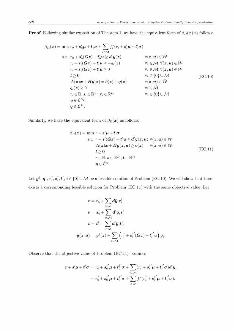
ec8 e-companion to Bertsimas et al.: Adaptive Distributionally Robust Optimization
Proof. Following similar exposition of Theorem 1, we have the equivalent form of βD(x) as follows:
βD(x) = min r0 + s′0µ+ t′0σ+∑i∈M
f∗i (ri + s′iµ+ t′iσ)
s.t. r0 + s′0(Gz) + t′0u≥ d′y(z) ∀(z,u)∈ W
ri + s′i(Gz) + t′iu≥−qi(z) ∀i∈M,∀(z,u)∈ Wri + s′i(Gz) + t′iu≥ 0 ∀i∈M,∀(z,u)∈ Wt≥ 0 ∀i∈ {0}∪MA(z)x+By(z) = b(z) + q(z) ∀(z,u)∈ Wqi(z)≥ 0 ∀i∈ Mri ∈R,si ∈RL1 , ti ∈RI2 ∀i∈ {0}∪My ∈LN2
q ∈LM .
(EC.10)
Similarly, we have the equivalent form of βE(x) as follows:
βE(x) = min r+ s′µ+ t′σ
s.t. r+ s′(Gz) + t′u≥ d′y(z,u) ∀(z,u)∈ WA(z)x+By(z,u)≥ b(z) ∀(z,u)∈ Wt≥ 0
r ∈R,s∈RL1 , t∈RI2y ∈ LN2 .
(EC.11)
Let y†, q†, r†i ,s†i , t†i , i∈ {0}∪M be a feasible solution of Problem (EC.10). We will show that there
exists a corresponding feasible solution for Problem (EC.11) with the same objective value. Let
r = r†0 +∑i∈M
dyir†i
s = s†0 +∑i∈M
d′yis†i
t = t†0 +∑i∈M
d′yit†i ,
y(z,u) = y†(z) +∑i∈M
(r†i + s†i
′(Gz) + t†i
′u)yi.
Observe that the objective value of Problem (EC.11) becomes
r+ s′µ+ t′σ = r†0 + s†0′µ+ t†0
′σ+
∑i∈M
(r†i + s†i′µ+ t†i
′σ)d′yi
= r†0 + s†0′µ+ t†0
′σ+
∑i∈M
f∗i (r†i + s†i′µ+ t†i
′σ).
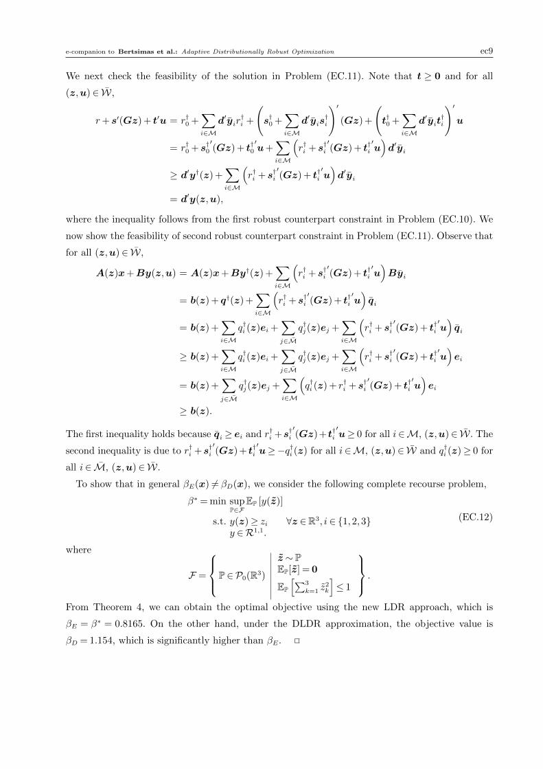
e-companion to Bertsimas et al.: Adaptive Distributionally Robust Optimization ec9
We next check the feasibility of the solution in Problem (EC.11). Note that t ≥ 0 and for all
(z,u)∈ W,
r+ s′(Gz) + t′u = r†0 +∑i∈M
d′yir†i +
(s†0 +
∑i∈M
d′yis†i
)′(Gz) +
(t†0 +
∑i∈M
d′yit†i
)′u
= r†0 + s†0′(Gz) + t†0
′u+
∑i∈M
(r†i + s†i
′(Gz) + t†i
′u)d′yi
≥ d′y†(z) +∑i∈M
(r†i + s†i
′(Gz) + t†i
′u)d′yi
= d′y(z,u),
where the inequality follows from the first robust counterpart constraint in Problem (EC.10). We
now show the feasibility of second robust counterpart constraint in Problem (EC.11). Observe that
for all (z,u)∈ W,
A(z)x+By(z,u) = A(z)x+By†(z) +∑i∈M
(r†i + s†i
′(Gz) + t†i
′u)Byi
= b(z) + q†(z) +∑i∈M
(r†i + s†i
′(Gz) + t†i
′u)qi
= b(z) +∑i∈M
q†i (z)ei +∑j∈M
q†j(z)ej +∑i∈M
(r†i + s†i
′(Gz) + t†i
′u)qi
≥ b(z) +∑i∈M
q†i (z)ei +∑j∈M
q†j(z)ej +∑i∈M
(r†i + s†i
′(Gz) + t†i
′u)ei
= b(z) +∑j∈M
q†j(z)ej +∑i∈M
(q†i (z) + r†i + s†i
′(Gz) + t†i
′u)ei
≥ b(z).
The first inequality holds because qi ≥ ei and r†i +s†i′(Gz)+ t†i
′u≥ 0 for all i∈M, (z,u)∈ W. The
second inequality is due to r†i +s†i′(Gz) + t†i
′u≥−q†i (z) for all i∈M, (z,u)∈ W and q†i (z)≥ 0 for
all i∈ M, (z,u)∈ W.
To show that in general βE(x) 6= βD(x), we consider the following complete recourse problem,
β∗ = min supP∈F
EP [y(z)]
s.t. y(z)≥ zi ∀z ∈R3, i∈ {1,2,3}y ∈R1,1.
(EC.12)
where
F =
P∈P0(R3)
z ∼ PEP[z] = 0
EP
[∑3
k=1 z2k
]≤ 1
.
From Theorem 4, we can obtain the optimal objective using the new LDR approach, which is
βE = β∗ = 0.8165. On the other hand, under the DLDR approximation, the objective value is
βD = 1.154, which is significantly higher than βE.
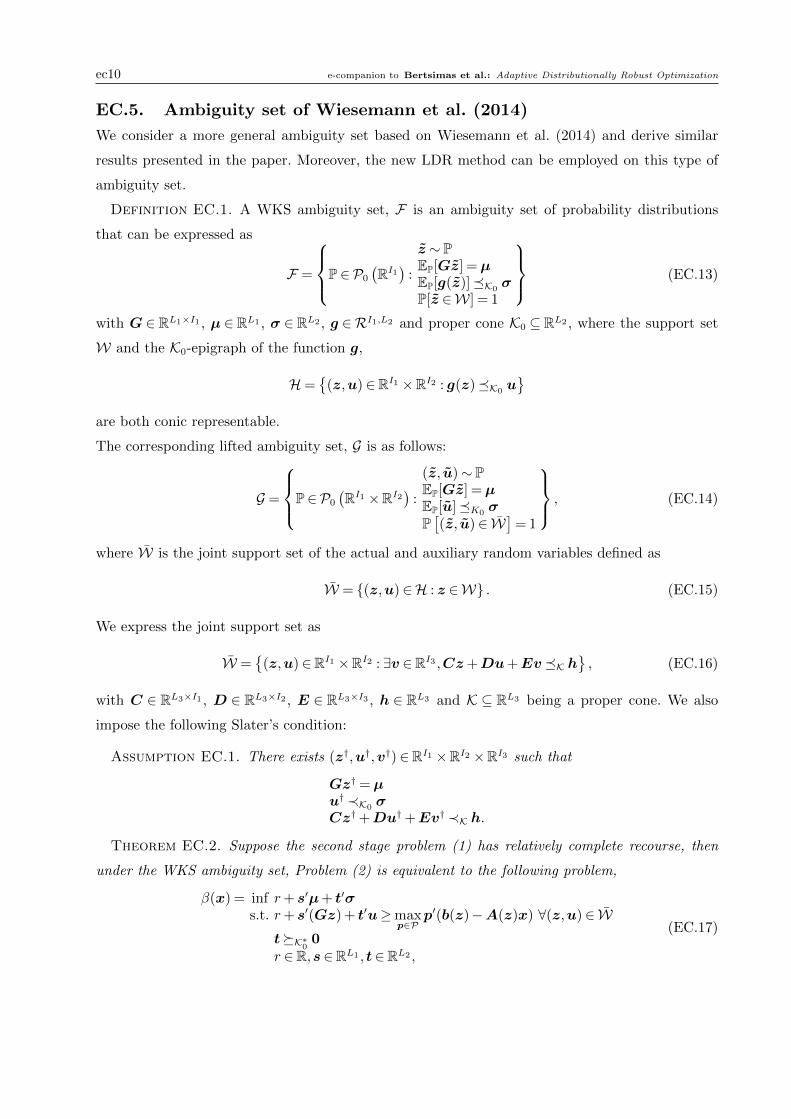
ec10 e-companion to Bertsimas et al.: Adaptive Distributionally Robust Optimization
EC.5. Ambiguity set of Wiesemann et al. (2014)
We consider a more general ambiguity set based on Wiesemann et al. (2014) and derive similar
results presented in the paper. Moreover, the new LDR method can be employed on this type of
ambiguity set.
Definition EC.1. A WKS ambiguity set, F is an ambiguity set of probability distributions
that can be expressed as
F =
P∈P0
(RI1)
:
z ∼ PEP[Gz] =µEP[g(z)]�K0
σP[z ∈W] = 1
(EC.13)
with G ∈ RL1×I1 , µ ∈ RL1 , σ ∈ RL2 , g ∈RI1,L2 and proper cone K0 ⊆ RL2 , where the support set
W and the K0-epigraph of the function g,
H={
(z,u)∈RI1 ×RI2 : g(z)�K0u}
are both conic representable.
The corresponding lifted ambiguity set, G is as follows:
G =
P∈P0
(RI1 ×RI2
):
(z, u)∼ PEP[Gz] =µEP[u]�K0
σP[(z, u)∈ W
]= 1
, (EC.14)
where W is the joint support set of the actual and auxiliary random variables defined as
W = {(z,u)∈H : z ∈W} . (EC.15)
We express the joint support set as
W ={
(z,u)∈RI1 ×RI2 : ∃v ∈RI3 ,Cz+Du+Ev�K h}, (EC.16)
with C ∈ RL3×I1 , D ∈ RL3×I2 , E ∈ RL3×I3 , h ∈ RL3 and K ⊆ RL3 being a proper cone. We also
impose the following Slater’s condition:
Assumption EC.1. There exists (z†,u†,v†)∈RI1 ×RI2 ×RI3 such that
Gz† =µu† ≺K0
σCz†+Du†+Ev† ≺K h.
Theorem EC.2. Suppose the second stage problem (1) has relatively complete recourse, then
under the WKS ambiguity set, Problem (2) is equivalent to the following problem,
β(x) = inf r+ s′µ+ t′σs.t. r+ s′(Gz) + t′u≥max
p∈Pp′(b(z)−A(z)x) ∀(z,u)∈ W
t�K∗0 0r ∈R,s∈RL1 , t∈RL2 ,
(EC.17)

e-companion to Bertsimas et al.: Adaptive Distributionally Robust Optimization ec11
where P is the dual feasible set of the Problem (1) given by
P ={p∈RM+ : B′p= d
}.
The explicit formulation is given by
β(x) = min r+ s′µ+ t′σs.t. r≥πi′h+pi
′b0−pi′A0x ∀i∈ [P ]
C ′πi =
p′i(b1−A1x)
...p′i(b
I1 −AI1x)
−G′s ∀i∈ [P ]
D′πi =−t ∀i∈ [P ]E′πi = 0 ∀i∈ [P ]πi �K∗ 0 ∀i∈ [P ]t�K∗0 0r ∈R,s∈RL1 , t∈RL2
πi ∈RL3 ∀i∈ [P ].
(EC.18)
where p1, . . . ,pP are the extreme points of P.
Proof. We leave this to the readers as the steps of the proof is identical to the proof of Theorem
1.