1

“Adaptive Digital Linearisation of High Power

Amplifier for Linear Modulation ”

Name: Nima Safari Sirdani

Supervisor in Chalmers University of Technology: Professor Tony Ottosson, Department of Signals & Systems.

Supervisor in Nera Telecommunications:

Professor Terje Roste, Nera Research.

Presentation Date: Wed. th3 Dec. 2003.

2

Abstract

M-QAM modulation has been considered to achieve high bandwidth efficiency for wireless communications. However, due to its envelope fluctuation, it exhibits large spectral regrowth and performance degradation when the transmit power amplifier (PA) operates in a non-linear region close to saturation. In this thesis, two different Adaptive Predistorters (PD) are evaluated and a new algorithm is introduced which shows faster convergence when there is no prior information about the PA characteristics. Spectrum Analysis and Transmission Quality are considered using the proposed adaptive predistorters. Two criterions are used to evaluate the PD performance, namely, Adjacent Channel Power Ratio (ACPR) and Error Vector Magnitude (EVM). The received 16-QAM symbols are compared with and without PD in AWGN channel and about 4 dB improvement in power efficiency is achieved in Output Back Off (OBO) of about 5.5 dB below saturation. A more efficient scheme for DSP implementation is presented with simulation results. Finally, a static PD based on a 64-entry table look-up is designed for a particular measured Class AB High Power Amplifier (HPA) and implemented by DSP processors in baseband and about 15 dB improvement in Adjacent Channel Power Ratio, is obtained and observed by Spectrum Analyser.

3

Contents 1. Introduction 2. Power Amplifier Modelling

2.1 Static and Memoryless Model for the Amplifier 2.2 Nonlinearity and Intermodulation Distortion 2.3 With-Memory Model for the Amplifier 3. System Model in Baseband

3.1 Linear Modulation and Filtering 3.2 Predistortion 3.3 High Power Amplifier

4. Adaptive Predistortion Algorithms 4.1 Discussion on different algorithms 4.2 Look Up Table (LUT) based method 4.2.1 Access or mapping 4.2.2 Update 4.2.3 Discussion on Stability and Convergence 4.2.4 Simulation Results

4.3 Parametric Based Method 4.3.1 Theory 4.3.1 Simulation results 4.4 Hybrid Method 4.5 Brief Discussion on with-Memory Predistortion 5. Discussion on Transmission Quality using Predistortion 5.1 Predistorter effects on Received Symbols 5.2 Predistorter effects on Received Symbols in AWGN channels 6. Discussion on Implementation Considerations

6.1 Implementation Approximations and Simulation Results 6.2 How to select the efficient Over-sampling rate 6.3 Effects of DAC and Reconstruction Filters on Predistorter

7. DSP implementation and Experimental results 7.1 Introduction to fixed-point DSP implementation 7.1 PA characteristic measurement and Predistortion Design 7.2 Experimental Results

8. Conclusion References Appendix List of Programs (.m files, .c++ files and .dsp files)

4

1. Introduction

Power Amplifiers (PAs) have become a bottleneck for modern telecommunication systems. Their purpose is to amplify the signal before transmitting it, and since relatively high power levels are used, they are major power consumers while doing this. Since all other electronic and digital signal processing (DSP) in a handset or terminal usually operate at much lower power levels, the total efficiency of the system is significantly determined by the efficiency of the PA at the time of transmitting. This means that the operating time in a handset is greatly dependent on the efficiency of the PA, while high efficiency is also preferred in base stations in order to achieve low power consumption and avoid problems of overheating. From a PA point of view, the difficulties in modern telecommunication systems arise from spectral efficiency. The number of users is increasing rapidly, and at the same time high data-rates have become a more and more important issue, as moving pictures and other data-expensive applications are gaining in popularity. This means that a full spectrum is expensive, and attempts are being made to transmit the maximum amount of data using the minimum amount of spectrum. Power Amplifiers (PA) is a major source of nonlinearity in a communication system. The nonlinear charateristics of a power amplifier can be represented by their AM/AM and AM/PM effects[1]. The AM/AM curve indicates the nonlinear relationship between the output and input envelope (or power). The AM/PM curve shows the output phase shift dependent on the input envelope (or power). They are therefore only suitable for constant envelope modulated signals e.g. MSK, GMSK, CPM, etc. Unfortunately, these modulations are less spectral efficient than linear modulations such as M_QAM, which produce a variation in both phase and the envelope of the signal. Due to their large envelope fluctuations, M_QAM signals require linear amplification to avoid spectral regrowth (broadening) and performance degradation. Normally the transmit power amplifier has to operate at a large output back off from its saturated power in order to maintain such linearity requirements. As a result, the power efficiency is very low (typically less than 10 %) and the heat dissipation is correspondingly high. Pre distortion techniques have been proposed as a potential solution to over come the nonlinear distortion effects. Basically these techniques aim to introduce ‘inverse’ nonlinearity that can compensate the AM/AM and AM/PM distortions generated by the nonlinear amplifier. These predistorters can be implemented in baseband by Digital Signal Processing (DSP) techniques. Since the amplifier characteristics, vary because of temperature changes and carrier frequency, the algorithm should be able to adapt itself with these variations. Here, we will start with amplifier modeling and the nonlinear effects on transmitted signal in chapter 2. The baseband model for adaptive predistortion is presented in chapter 3. In chapter 4, we discuss about the adaptive algorithms and the simulation results are presented. Predistortion effects on transmission quality are discussed in chapter 5 and finally in the last two chapters, some considerations for implementation and the experimental results are presented and discussed.

5

2. Power Amplifier Modelling 2.1 Static and Memoryless Model for the Amplifier

Power Amplifiers are important elements in radio communications systems and they are inherently nonlinear. A system is considered to be nonlinear if the output is a nonlinear function of the input. There are a number of ways of modelling the nonlinearity of a system, one of the most useful way is polynomial modelling. The power series model or the polynomial model is widely used in the literature to describe nonlinear effects in power amplifiers. Let’s denote the baseband equivalent PA input signal and PA output signal, by

)(tx and )(ty respectively. We can approximate the memoryless PA output/input relationship by a polynomial [2]:

[ ] [ ]kK

kk

kkK

kk txatxtxtxaty

2

012

1

012 )()(*)()()( ∑∑

=+

+

=+ == (1)

Where the polynomial coefficients, 12 +ka , are generally complex-valued, except when there is no AM/PM conversion. Thus the complex gain of the amplifier is:

kK

kk ra

txtyrG

2

012)(

)()( ∑=

+== which is a function of input amplitude )(txr = .

Therefore ⎪⎩

⎪⎨

⎧

Φ+=

=

)(

)()()(

r

rAtxty

xy θθ,

Where Φ,A indicate the AM/AM and AM/PM transfer function of the amplifier. So, given the AM/AM and AM/PM data, one can easily obtain the complex gain

)()()( rGjerGrG ∠= . Next, a least squares fit of G(r) yields the polynomial coefficients

12 +ka , for our polynomial complex gain model. Third order intercept point (IP3), fifth order intercept point (IP5), seventh order intercept point (IP7), and 1 dB compression point (P1dB) are alternative measures of a PA. These quantities can be shown as a function of 7531 ,,, aaaa [3]. Therefore if instead of the AM/AM and AM/PM characteristics, IP3, IP5, IP7 and P1dB data are available, we can solve a system of equations to obtain the PA polynomial coefficients.

6

2.2 Nonlinearity and Intermodulation Distortion

In this section, the effects of nonlinearity on signal’s spectrum are to be considered. Let’s show the Input-Output PA model as a simple 3rd order polynomial:

.33

221 xaxaxay ++= (2)

where 321 ,, aaa are complex coefficients. If a two tone signal, )cos()cos( 21 twtwx ⋅+⋅= , is applied as the input, several new spectral components are generated in the output because of nonlinearity. Figure 1 shows the input and output spectrum.

Some of the unwanted spectral components, such as harmonics, can be easily filtered out, and the same conclusion can be reached regarding the DC band. The situation is completely different for the third order Intermodulation (IM3) components, which are so close to the carrier that they cannot be filtered. The difference between the level of main components and the level of intermodulation components, which denoted by ACPR (Adjacent Channel Power Ratio) is a figure of merit for linearity. The situation is the same for a band pass pulse. If we denote X(f), Y(f) as the Fourier Transform of Input and Output respectively, from (2) we have:

...)(*)(*)()(*)()()( 321 +++= fXfXfXafXfXafXafY where * denotes the convolution operator. Figure 2 shows a band pass sinc (band pass pulse in frequency domain) that is applied to a 3rd order nonlinear PA. Spectrum regrowth, as well as in-band distortion due to Intermodulation, can be seen.

Fig. 1

7

2.3 With-Memory Model for the Amplifier

There is an important drawback with polynomial input-output modelling, however, which is that the nonlinearity introduced by the system is only affected by the input amplitude and not by the frequency or bandwidth of the signal. This type of modelling is therefore called narrowband modelling, or narrowband approximation of the real system, which is always affected to some extent by the signal bandwidth. For wideband applications (e.g. in wideband CDMA) and/or with high power amplifiers (e.g. base stations PAs), memory effects show up in the PA [9], [22]. Memory effects are attributed to filter group delay, the frequency response of matching networks, non-linear capacitance of the transistors and the response of the bias network. Having memory means that the output of the PA is not only a function of the current input but also a function of the past inputs. A relatively simple baseband behavioural model that accommodates memory as well as nonlinear behaviour is described below [6]:

∑=

=−=

Mm

mmnmmn xbBy

0

),( (3)

where M is the maximum delay in the unit of sample, and

∑=

−−−− ⋅=

mP

k

kmnmkmnmnmm xbxxbB

1

1),(

PAnx ny

Fig. 2

8

where mP is the order of polynomial ),( mnmm xbB − . The components of vector b m , { }

mmPmm bbb ,..., 21 , are complex numbers. The fundamental difference between the nonlinearity and memory effects is that the nonlinearities generate new spectral components, while memory only shapes the existing signal components, i.e. memory can be considered as a filtering which may distort the whole or part of the signal spectrum. As mentioned before, memory effects show up in wideband transmission and are negligible in other cases. In [22], it was shown that, for bandwidth more than 5 MHz, this effects should be taken in to account. In this thesis, we focus on memoryless model for PA.

3. System Model in Baseband Figure 3 shows the baseband model for the adaptive precompensator [5]:

The factor α is the desired amplitude gain of the amplifier i.e. )()(

tXtZ

=α .

R/P means rectangular to polar coordinates conversion. X(t) denotes the signal after pule-shaping and Y(t) and z(t) are the baseband equivalent input and output signal of power amplifier, respectively. The output signal after envelope normalization and offset

0θ

M_QAM Symbol generator

R/P H(r)

)(rΨ

P/R FIR filter, for Pulse shaping

HPA

+

m

X(t) Y(t) Z(t)

α/1×

Σ Adaptive algorithm

-

Error

∧

)( tZ

τ

Predistorter

Fig. 3

9

phase cancellation, )(ˆ tZ , is contrasted with the appropriate input signal, X(t), to provide the amplitude and phase errors to feed the algorithm and update the predistorter.

3.1 Linear Modulation and Filtering

After M_QAM symbol generation, the symbols are sent to the pulse-shaping filter. This filter is designed so that optimum spectral concentration, lowest sidelobe of the filter, is achieved in the transmission bandwidth of the channel and zero Inter Symbol Interference (ISI) is obtained. For baseband transmission, using squared root raised cosine wave, the maximum

spectral concentration should occur in the region ( )⎥⎦⎤

⎢⎣⎡ ++−

TT 21,

21 αα , where

T1 denotes

the symbol rate and α is the roll off factor, determines the excess bandwidth allowed.

Parameters of the filters are the number of coefficients L and the sampling rate TN s ,

where sN is an integer over-sampling factor. Consider the figure below, the L-tap transmitter filter is characterized by the coefficient

vector [ ]TNpppP 110 ,...,, −= and is clocked at rate TN s . Every T seconds an

information ‘ na ’ enters the transmitter filter followed by 1−sN zeros.

… The filter coefficients are obtained to maximize the spectral concentration, [10] as:

( )[ ] ( )[ ]( ) tt

tttPi )41(1cos41sin

2απαπααπ

−+⋅+−

= (4)

{ },...0,0,,...,0,0, 1+nn aa

∑

0p

M_QAM samples

1−Lp

10

where sN

Lit 2/)1( −−= .

For the given roll off factor,α , and over-sampling rate sN , the achievable spectral concentration increases with filter length. In simulations, a sN×10 -tap filter is used to have an acceptable spectral concentration with roll off factor of 25.0=α . Figure 4 shows the 16-QAM samples after filtering. It can be seen that the peak power (or envelope) of filtered samples are much larger than the average power (or amplitude). It is found that the peak to average ratio, with the roll off factor of 25%, is about 6 dB in 16-QAM modulation.

3.2 Predistortion

After filtering the TX signal are predistorted in a way that the combination of predistorter and the non-linear amplifier makes a linear amplification. In fact, the predistorter aims to get the inverse of the amplifier complex gain characteristics. When the signal bandwidth increases, amplifiers show some memory effects in their characteristics, and with-memory predistorters is needed to compensate for the nonlinearity and memory effect of amplifiers. Predistortion can be introduced by static or adaptive algorithms. Static algorithms are simple but sensitive to amplifier characteristic variations. Adaptive algorithms are more

Fig. 4

11

complex since feedback line (as figure 5 shows) is required to find the error and feed the algorithm to adapt to variations. In this thesis we focus on adaptive memoryless algorithm for predistortion which is fully investigated in next chapter. However, a brief discussion on memory effect cancellation is also made in next chapter. Let’s consider Figure 5:

⎩⎨⎧

==

)()(

YfZXgY

where g and f are the complex function of PD and PA respectively.

The overall desired characteristic is: XZ α= , where α is the real valued gain. Since XXgfYfZ α≈== ))(()( ⇒ )()( 1 XfXg α−≈ . Thus the desired function for the predistorter is the inverse of normalised version (by α ) of f(.). i.e. if we denote

ffα1ˆ = , then

fg

ˆ1

= and fg ˆ−∠=∠ .

If 0ˆ →−=− XZerrorAmplitude ⇒ XZ →ˆ ⇒ XZ α→ ,

And for the phase we have: |))((|)()( XgXgXYYZ Φ+∠+∠=Φ+∠=∠ , where (.)Φ is the AM/PM characteristic of the amplifier.

Therefore if 0|))((|)( →Φ+∠=∠−∠=−∧

XgXgXZerrorPhase ⇒ |))((|)( XgXg Φ−→∠ , and the phase shift introduced by amplifier is compensated.

3.3 High Power Amplifier

Here, we are to define some parameters to deal with the non-linear amplifier: It is quite difficult to linearize the power amplifier up to its saturated output power Psat [4]. Thus the maximum output power of the linearized power amplifier is S.Psat where 0<S<1. S represents the Peak BackOff (PBO) of the power amplifier. [4]:

)(log10 10 SPBO −= .

HPA

+

X Y Z

α/1×

Σ Adaptive algorithm

-

Error

g (.)

PD

f(.)

ZFig. 5

12

Here, for simplicity we normalize the input amplitude, thus, 0<r<1 and the amplitude gain of the amplifier is:

PsatS ⋅=α . Thus, the choice of α determines the minimum PBO of the proposed predistorter. The output backoff (OBO) in dB is defined as [4]:

)(log10)(log10 1010 PPsatOBO −= , where P is the average power of the transmitted signal. Large OBO value implies inefficient operation. Note that the amplifier output power cannot exceed its saturation value. The best possible characteristic of the combined predistorter and amplifier is therefore that of a limiter having an output signal proportional to the input signal with slope α . The effect of the gain α , is simply to change the range of the input, that is, the input amplitude r at which the amplifier saturates. Figure 6 shows the normalized characteristic of a class AB HPA obtained by tone measurements. Line (1) show the parameter S, which corresponds to a certain PBO (or a certain OBO for a fixed modulation scheme). If the input range varies (e.g. from 1r to

2r ) then the overall gain changes (from 1gain to 2gain ) keeping the output level unchanged. For the specified output level, therefore, the desired predistorted output amplitude will be between [ ]outrd,0 (as the figure shows), which corresponds to the maximum phase shift shown by line 2.

The amplifier model for the simulations is assumed to obey the ‘arctan’ model [9]:

( ) ( )[ ] )(2

121

11 )(tan)(tan)( tYjetYtYtZ ∠−− += ηγηγ (5),

Fig. 6

13

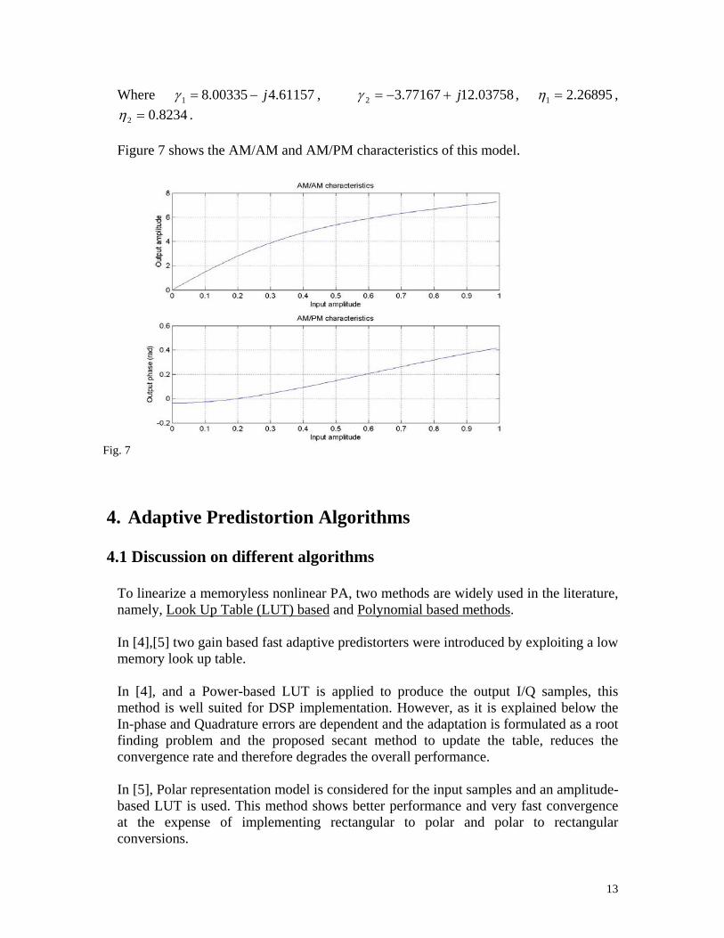
Where 61157.400335.81 j−=γ , 03758.1277167.32 j+−=γ , 26895.21 =η , 8234.02 =η .

Figure 7 shows the AM/AM and AM/PM characteristics of this model.

4. Adaptive Predistortion Algorithms 4.1 Discussion on different algorithms

To linearize a memoryless nonlinear PA, two methods are widely used in the literature, namely, Look Up Table (LUT) based and Polynomial based methods. In [4],[5] two gain based fast adaptive predistorters were introduced by exploiting a low memory look up table. In [4], and a Power-based LUT is applied to produce the output I/Q samples, this method is well suited for DSP implementation. However, as it is explained below the In-phase and Quadrature errors are dependent and the adaptation is formulated as a root finding problem and the proposed secant method to update the table, reduces the convergence rate and therefore degrades the overall performance. In [5], Polar representation model is considered for the input samples and an amplitude-based LUT is used. This method shows better performance and very fast convergence at the expense of implementing rectangular to polar and polar to rectangular conversions.

Fig. 7

14

In [6], a Polynomial model used for the Predistorter in order to compensate for the AM/AM and AM/PM characteristics of the amplifier and a simple and fast converging method obtained by using LMS algorithm to estimate the polynomial coefficients. An I/Q represented polynomial method based on adjacent channel emission measurement was introduced in [7]. Another adaptive polynomial I and Q predistorter was presented in [8], which shows a good convergence rate and a high reduction in spectrum spreading. In [8] a combination of analog predistorter and postdistorter was used to improve the convergence rate. Before going through the algorithms, it is worthwhile to discuss about the input and output data formats used before and after PD. Input samples in PD can be represented in two different formats: I/Q representation or Polar representation formats. Here we discuss the performance of PD based on these two formats. Let’s consider the table below, which can be used as a mapping Predistorter: In this case, In-phase and Quadrature part of input sample is used to find the index of appropriate output. As the figure shows all the entries on the circle e.g. C have the same amplitude and all the entries on the line e.g. L have the same phase. This redundancy information makes the table very large and increases the computation load, and in consequence degrades the performance and convergence rate as well. As we don’t need the information about the input phase to linearize the amplifier, an alternative and much better solution is to tolerate a few computations and to use the input amplitude or input power to access the appropriate output. The output of table may be represented either in I/Q format or in polar format.

LC

Q

I

15

Let’s consider figure below as the baseband normalised model for the Predistortion adaptive algorithm in rectangular representation. Where )(~),(~ rrA Φ represents the AM/AM and AM/PM conversions of predistorter and

)(),( rrA Φ shows the amplitude and phase characteristics of power amplifier, respectively. We have:

injerX θ⋅= as the input of predistorter.

[ ])|)(|sin()|)(|cos(|)(||)(| )|)(|( YYjYYYAeYAZ YYj ∠+Φ+∠+Φ== ∠+Φ , Y= ))(~()(~

inrjerA θ+Φ . Thus the In-phase and Quadrature errors can be calculated as:

[ ]

[ ]⎪⎩

⎪⎨

⎧

−=−=

−=−=

outQQQQ

outIIII

rAAXZXe

rAAXZXe

θ

θ

sin.)(~

cos.)(~

where [ ] inout rrA θθ +Φ+Φ= )(~)(~ . As the calculation shows, I and Q errors are dependent and some methods should be applied to minimise them together.

+

Y Z

Σ Adaptive algorithm

-

Error

PD PA

)(~),(~ rrA Φ )(),( rrA Φ

injerX θ.=

Fig. 8

16

[ ] 0)(~)(~=Φ+Φ rrA and inout θθ = ,

If 0, →QI ee ⇒

[ ] rrAA =)(~ . Which are the conditions to linearize the amplifier. Thus, this method is very simple in mapping, because there is no need to implement p/r conversions at the output of PD. However, to satisfy linearisation conditions, complex iterative methods needed, and the gradient estimation, which minimizes the mean-square error, may not provide a sufficiently rapid rate of convergence or a sufficiently small excess mean-squared error. Thus, the complex and slow adaptation, is the main drawback with this case. In the other case, the polar representation method is more complex in mapping, since the predistortion requires polar representation, but of course much simpler in table updating since the phase and amplitude errors are independent and simple linear methods e.g. LMS can provide a fast convergence. Since the evaluation of a predistortion technique should take into account both its performance and complexity, polar representation based methods seems to be a better choice in adaptive Predistorters. Here, both the LUT based and polynomial-based methods are analyzed theoretically and evaluated by simulations. In both methods polar representation of input data is assumed.

4.2 Look Up Table (LUT) based method

In this method, a polar represented table is used to make the complex function for the predistorter as shown below. Input xi

ii erX θ= is converted to )(|| idxji ed θθ + .

Input Amplitude

Output Amplitude

Output Phase

r1 d1 1dθ r2 d2 2dθ r3 d3 3dθ

nr dn dnθ

≈≈

iX iY

Fig. 9

17

4.2.1 Access or mapping

Since it takes a huge amount of memory to save all the possible input amplitudes, Linear Interpolation is used to find the output amplitude and phase, e.g. if || iX is between kr and 1+kr , then the table output amplitude and phase will be:

( )

( )⎪⎪⎩

⎪⎪⎨

⎧

∠+−−

−+=∠

−−−

+=

+

+

+

+

ikikk

dkddki

kikk

kkki

XrXrr

Y

rXrrdd

dY

k ||

||||

1

1

1

1θθ

θ

This signal, then passes through the non-linear power amplifier to generate the amplified signal, Z.

4.2.2 Update

The algorithm should be able to identify the amplifier characteristics and update the table to adapt with the variation of PA characteristics. Table updating is based on minimising the error, defined as the difference between Input and the Normalised Output. Thus, the thk and thk 1+ entry of the table are updated as follow:

⎩⎨⎧

⋅∆⋅+=

⋅∆⋅+=

++++

+

)()(

1,1,1,1

,,,1

iESddiESdd

akiakiki

akiakiki (6)

Where ( )iia ZXiE ˆ)( −= is the amplitude error in thi sample, aS is to control the

convergence rate and the stability and∆ is used to weight the updating values, and the idea is, the entry closer to the input value gets the larger share of error and is defined as:

⎪⎪

⎩

⎪⎪

⎨

⎧

−=∆

−=∆

+

+

sizesteprX

sizesteprX

kiki

kiki

_

_

1,

1,

(7)

And the step_size is defined by the ratio of input amplitude range and the memory size, if the input amplitude is normalised then, step_size=1/(memory_size). The same steps are done for phase table updating. Let’s define: )(iE p as the error in thi sample, ( )iip ZXiE ˆ)( ∠−∠= .

Then, thk and thk 1+ entry of the table are updated as:

⎪⎩

⎪⎨⎧

⋅∆⋅+=

⋅∆⋅+=

++++

+

)()(

1,1,1,1

,,,1

iESiES

pkipkiki

pkipkiki

θθ

θθ (8)

where the parameter pS is to control the convergence rate and the stability.

18

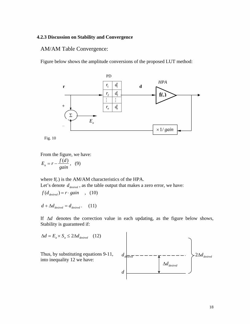
4.2.3 Discussion on Stability and Convergence

AM/AM Table Convergence: Figure below shows the amplitude conversions of the proposed LUT method:

1r 1d

2r 2d M M

nr nd

From the figure, we have:

gaindfrEa

)(−= , (9)

where f(.) is the AM/AM characteristics of the HPA. Let’s denote desiredd , as the table output that makes a zero error, we have:

gainrdf desired ⋅=)( , (10)

desireddesired ddd =∆+ . (11) If d∆ denotes the correction value in each updating, as the figure below shows, Stability is guaranteed if:

desiredaa dSEd ∆≤×=∆ 2 (12) Thus, by substituting equations 9-11, into inequality 12 we have:

PD HPA

+

r d

gain/1×

Σ

-

f(.)

Fig. 10

aE

desiredd

desiredd∆

d

desiredd∆2

19

[ ]ddSgain

dfdfdesireda

desired −≤×⎥⎦

⎤⎢⎣

⎡ − 2)()( ⇒ [ ] gainSdd

dfdfa

desired

desired ×≤×⎥⎦

⎤⎢⎣

⎡−− 2)()( .

Where [ ] ⎥⎦

⎤⎢⎣

⎡−−

dddfdf

desired

desired )()( represents the differential gain of HPA around desiredd .

Therefore, the stability depends on the dynamic slop of the AM/AM characteristics of the power amplifier and the desired gain. And to guarantee the stability the control parameter aS should be selected as: (13) And the optimum speed of convergence for a given differential gain occurs at half of this value. AM/PM Table Convergence: The same steps can be done for the phase convergence: If we denote (.)Φ as the AM/PM characteristics of the amplifier, and dθ as the output of table, the phase error can be obtained as:

[ ]dp dE θ+Φ−= )( , If 0→pE , then )(d

desiredd Φ−=θ The stability is guaranteed if

)(2 ddpp desiredSE θθθ −≤×=∆

Therefore, (14) And 1=pS , gives the quickest convergence. It is worth to mention that, the amplitude stability is the necessary condition for the phase convergence. Simulations based on the described algorithm are presented in the next section.

amplifier theofgain aldifferenti .max2 gainS a×

≤

2≤pS

20

4.2.4 Simulation Results

The simulation was done under the following assumptions: 1-Arc tan model is assumed for the amplifier, and the input amplitude is normalized. 2-Step size of the table was Uniform and the size of the amplitude and phase table is assumed to be equal. 3-At the beginning the amplitude table is assumed to be transparent and all phase shift output entries are set to zero. (i.e. Y(t)=X(t)) 4-FIR filter length is 10 symbols, over-sampling rate of 8 sample per QAM symbols, and the rolloff factor equal to 0.25. Figure 11 shows the amplitude and phase error and the trained table for 16-QAM with table size of 32 and the mentioned PA model. Peak Back Off factor (S) is assumed 0.9 i.e. PBO=0.457 dB, saturated Voltage according to the model is Vsat=10 and the gain is 9.5 (about 9.8 dB).

It is seen that the algorithm could almost find the inverse function of PA AM/AM and AM/PM characteristics. And the error vanished after about 2000 samples. However some peaks are observed even after 4000 samples. The reason is related to the Non-Uniform distribution of input amplitude. Since we don’t have enough samples in very low and very high amplitude, the table entries in those regions aren’t trained. There are sevaral solutions to overcome this effect and to increase the convergence rate. Here we evaluate some of these solutions and in the next sections a much simpler way is introduced to cope with this problem. The idea is to choose a smarter initialization for the amplitude and phase look up table. Figure 12 illustrates the output spectrum with and without predistorter in comparison to the input signal.

Fig. 11

21

As figure shows, the non-linear amplifier causes spectral regrowth as well as in-band distortion. Using predistorter, it is seen that about 20 dB improvement in adjacent channel power ratio is obtained.

There is a drawback in the algorithm described above. It was seen that sometimes abrupt changes in the table, specially in training time, might cause a gap or peak and degrade the performance or make the convergence very slow, when we update only the two nearest points by each sample. Thus we decided to increase the updated points to 4 and the weights in equation (7) will change as following steps:

1- Find the distances between the input amplitude and 4 nearest points in the table: mii rXmdis −=)( m=1,2,3,4

2- Find the inverse of distances ()(

1mdisi

).

3- Find the updating weight for each index:

∑=

=∆ 4

1

,

)(1

)(1

m i

imi

mdis

mdis

This modification made the algorithm more stable and faster to converge but increases the table updating computations. Thus we still are seeking a better method.

Fig. 12

20dB

22

As said before, since the amplitude of the QAM samples are not uniformly distributed, some regions in the table may converge slowly. Thus the idea of designing a training or calibrating signal, which uniformly cover the whole range of the sample’s amplitude, seems to be nice. [12] Another solution to increase the convergence rate is to optimize the table size. It is seen that a high table size decreases the convergence rate and a low table size causes a large steady state error both in amplitude and phase. Thus, exploiting a low size in training time to make a fast convergence and increasing the table size to have a small enough error may be a worthwhile idea to test. Figure 13 shows the simulation results for a variable size look up table. In this case we start from a 16-entry table and finish with a 32-entry table. The criterion to switch from 16-entry table into 32-entry table was the mean squared amplitude and phase error. As the amplitude and phase error shows the convergence rate highly improved in comparison to figure 11.

Till now, we employed uniform spacing of the PD lookup table entries. Thus the question of optimum nonuniform spacing remains unsolved. In [11], the author derived a systematic way to describe and analyze arbitrary non-uniform spacing of PD table entries; and simple expression for the optimum non-uniform spacing and its performance. It is shown in the paper that making predistortion tables equispaced in amplitude is an excellent choice from an engineering stand point: it is simple, it does not depend on amplifier, modulation format or backoff, and its performance is very close to the limit defined by optimum spacing. In conclusion, we have seen that, simple amplitude-based uniform spacing look up table method, is a practical and near-optimum choice to linearize the amplifier and to remove the power spectrum distortion and expansion. However, slow convergence rate, degrades the performance and increases the probability of making error. Some methods were introduced to solve this problem and the simulation results were given. In the next section, a simple parametric model is considered to compensate the PA nonlinearity.

Fig. 13

23

4.3 Parametric Based Method

4.3.1 Theory: Let’s denote F(.) and P(.) as the AM/AM and AM/PM characteristics of Predistorter and r=|X|, the input amplitude. From our previous discussions, we know that to linearise the amplifier the following expressions should be satisfied:

( )( )⎩

⎨⎧

=∠+

⋅==

0)()()(

rFfrPrrFfY α

Where f(.) in the complex function describing the amplifier characteristics. The amplitude and phase predistortion function, F, P can be modeled by:

⎪⎩

⎪⎨⎧

=+++=

=+++=

pTm

m

fTl

l

RPrprpprP

RVrfrfrfrF

...)(

...)(

10

221 (15)

where

⎥⎥⎥⎥⎥

⎦

⎤

⎢⎢⎢⎢⎢

⎣

⎡

=

l

f

r

rr

RM

2

,

⎥⎥⎥⎥⎥

⎦

⎤

⎢⎢⎢⎢⎢

⎣

⎡

=

m

p

r

rR

M

1

, ⎥⎥⎥⎥

⎦

⎤

⎢⎢⎢⎢

⎣

⎡

=

lf

ff

VM

2

1

, ⎥⎥⎥⎥

⎦

⎤

⎢⎢⎢⎢

⎣

⎡

=

mp

pp

PM

2

1

.

The least mean square (LMS) algorithm is used to determine the optimum coefficients V of the amplitude predistorter and can be derived as follow [6]:

kvkfvikvkfT

kfkk eRVeRVfRVV ,,,,,1 )( µµ +=′+=+ (16)

where )( ,, kfT

kkkV RVfre −=α and )( ,kfT

v RVf ′⋅= µµ

And for the phase polynomial coefficients we have:

kppfpii eRPP ,,1 µ+=+ (17)

where )(ˆ,,, kf

Tkkp

TkkP RVfRPZXe ∠−−=∠−∠= .

The initial coefficients assumed as: [ ]TV 0,...,0,11 = [ ]TP 0,...,0,01 =

The step size (mu) controls the convergence rate and stability of the algorithm.

24

4.3.2 Simulation results

In this case the amplifier model is the same as one assumed in LUT method, and the PBO factors and any other parameters kept the same. The step size for the LMS algorithm is assumed 0.05 for the amplitude and 0.1 for the phase coefficient updating A five-order polynomial is considered for the phase and amplitude predistorter. Amplitude and Phase error are shown in Figure 14. As the Figure shows, the convergence is much faster in comparison to the LUT method.

Figure 15 shows the spectral analysis of the Polynomial predistorter. Like LUT method an improvement of about 20 dB is achieved using PD.

Fig. 14

Fig. 15

18dB

25

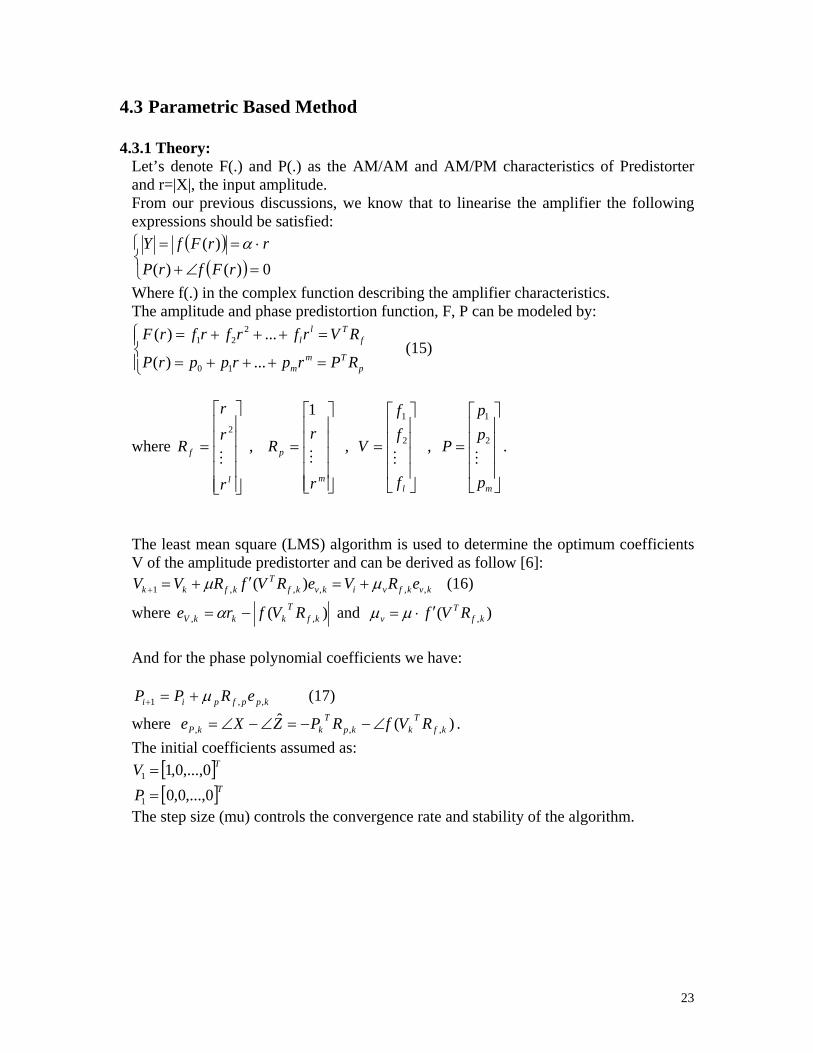
As observed, parametric method can find a very fast approximation of PA inverse function. However, we should mention that, some PA characteristics might not be described with a low order polynomial in a good approximation. In these cases, a high order polynomial is required as the predistorter function, which increases the computations and complexity. This test was done for some real models of the amplifier obtained based on tone measurement. The results were not so good as those shown above even with a large order, especially for the phase. The reason returns to the intrinsic behavior of the AM/PM characteristics, which may not be represented as a polynomial with good approximation. Figure 16 shows the results of applying polynomial method to the measured model for M_4 High Power Amplifier (Appendix A).

It means that this method can find a fast but not very exact approximation to the PA inverse function.

4.4 Hybrid Method

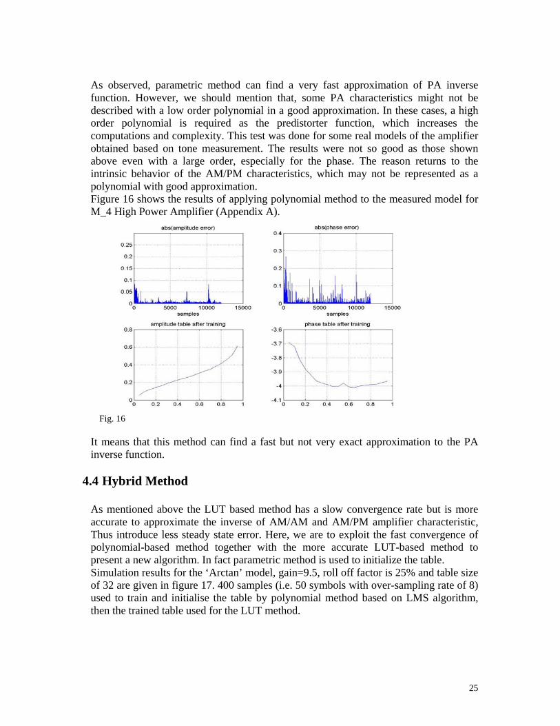
As mentioned above the LUT based method has a slow convergence rate but is more accurate to approximate the inverse of AM/AM and AM/PM amplifier characteristic, Thus introduce less steady state error. Here, we are to exploit the fast convergence of polynomial-based method together with the more accurate LUT-based method to present a new algorithm. In fact parametric method is used to initialize the table. Simulation results for the ‘Arctan’ model, gain=9.5, roll off factor is 25% and table size of 32 are given in figure 17. 400 samples (i.e. 50 symbols with over-sampling rate of 8) used to train and initialise the table by polynomial method based on LMS algorithm, then the trained table used for the LUT method.

Fig. 16

26

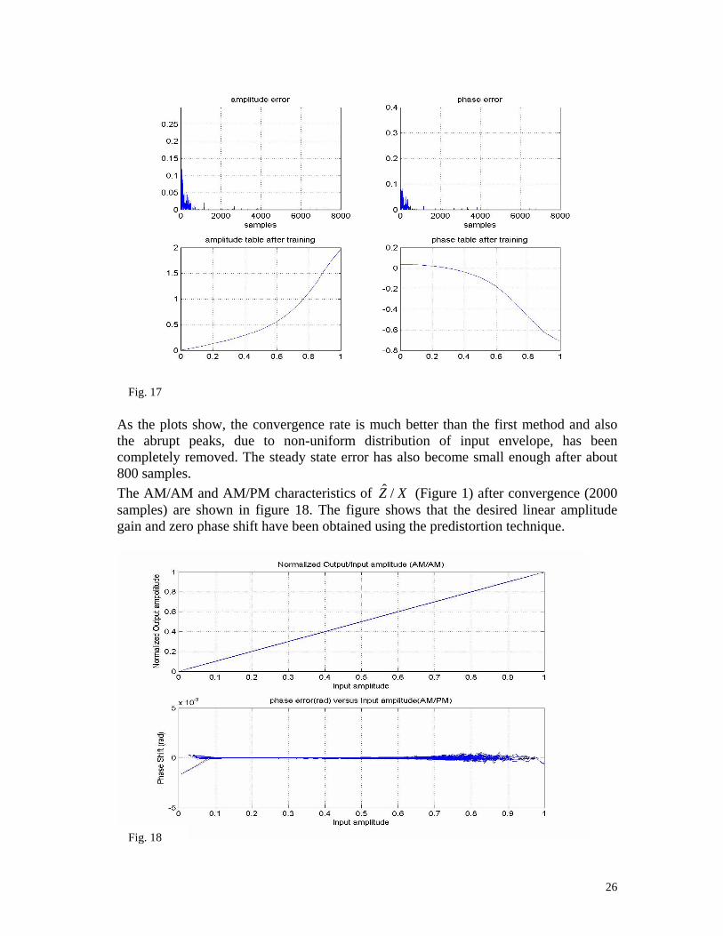
As the plots show, the convergence rate is much better than the first method and also the abrupt peaks, due to non-uniform distribution of input envelope, has been completely removed. The steady state error has also become small enough after about 800 samples. The AM/AM and AM/PM characteristics of XZ /ˆ (Figure 1) after convergence (2000 samples) are shown in figure 18. The figure shows that the desired linear amplitude gain and zero phase shift have been obtained using the predistortion technique.

Fig. 17

Fig. 18

27

4.5 Brief Discussion on with-Memory Predistortion

The performance of Digital Predistortion algorithms that do not take the memory effects in to account is severely degraded as the bandwidth of the input signal increases. Indeed, the exact inverse of a nonlinear system with memory should be another nonlinear system with memory. In [22-24], some algorithms have been introduced to compensate the with memory nonlinearity based on Volterra model Predistorter. With memory channel can be modelled as Wiener-Hammerstein (W-H) model; i.e. a linear time invariant (LTI) system followed by a memoryless nonlinearity, which in turn is followed by another LTI system [9]. Figure 19 shows the Indirect learning architecture for the Volterra series model Predistorter [23]. The Volterra series model Predistorter is expressed in a matrix form as: [ ] [ ]nXhnd T⋅=

where d[n] is the output of the Volterra model Predistorter, the superscript T denotes the transpose of the matrix, h is the Volterra kernel vector, and X[n] is the input vector. The overall system output y[n] is given by [ ] )(γfny = , where f is a nonlinear system function with memory and the vector γ is

given by:

[ ] [ ] [ ] [ ])1,...,2,1,( +−−−= Mndndndndγ . Here, M is the memory duration of the nonlinear system.

)(zH Memoryless NLPA )(zG

Volterra Model PD (copy of A)

Nonlinear System

Volterra Model PD (A)

+

-+

X[n] d[n] Y[n]

[ ] innovationn :α

Z[n]

G1

Fig. 19

28

The output Z of the training Volterra series model is given by:

[ ] [ ]nyhG

nZ T⋅=1 .

If the Volterra series models satisfy the following conditions, if [ ] [ ] ,/ Gnynx ≠ then [ ] [ ]nznd ≠ and if [ ] [ ] ,/Gnynx = then [ ] [ ]nznd = Then, as [ ]nα approach zero, y[n] approaches [ ]nxG ⋅ . [ ]nα , is called the innovation that represents the information contained in the current

desired output value which can not be predicted by the previous kernel vector. The modified RLS algorithm is used to update the training Volterra series system, as follow [23]:

[ ] [ ]nnkhh nn *)1()( α⋅+= −

[ ] [ ] [ ][ ] [ ] [ ]nynPny

nynPnk T

T

ˆ1ˆ1ˆ1

*1

1

−+−

= −

−

λλ

[ ] [ ] [ ] [ ] [ ]1ˆ1 *11 −−−= −− nPnynknPnP λλ

where [ ] [ ]Gnyny =ˆ .

We should mention that, with-memory PD techniques were not fully pursued here and are out of the scope of this thesis.

5. Discussion on Transmission Quality 5.1 Predistortion Effects on Received Symbols

In this section we are to observe the effects that nonlinearity may introduce to the symbols. By now, we have focused on Adjacent Channel Interference (ACI) criterion, here we consider another criterion which is widely used as a merit of transmission quality.

The mean squared estimate of Error Vector Magnitude (EVM) is defined as [13]:

( )2

1

0

22

2

1

mean

N

jjj

lin S

QIN

EVM∑−

=

+

=

δδ (17)

29

where Iδ and Qδ are the magnitude errors in the received data points (symbols) at the output of an ideal linear matched received filter. N is the number of data points (symbols) in the measurement sample. 2

meanS is the mean squared magnitude of the expected symbols over the same period. Figure 20 shows the symbol constellations after nonlinear amplification in OBO of 5 dB and the TX and RX filter length of 10 symbols and over-sampling rate of 8.

As the figure shows even without any noise, the symbols are scattered and phase rotated, which dramatically increases the error probability and degrades the system performance. Figure 21 Shows the noise free received 16-QAM symbols using PD from the beginning (Figure a) and after the convergence i.e. 200 symbols (Figure b).

Fig. 20: 16 QAM symbols without predistorter with OBO=5 dB and measured Class-AB-hpa, rotating and scattering effects are observed

(a) (b)

Fig. 21:16 QAM symbols using predistorter with PBO=0 dB, OBO=5.7 dB and Class-AB-hpa Overall [ ]%

2EVM =0.1207 and after the convergence [ ]%2EVM =0.0236

30

To eliminate the rotating effect in table training time, an offset phase estimator can be used to estimate the phase offset of the amplifier. The Offset phase can be easily estimated using the first sample or a few first samples as follow:

)_()_(0 sampleInputanglesampleoutputanglep −= . And this value is substituted in phase compensator polynomial model, equation (15), as 0p . This offset phase estimator may be very simple but in simulation, it works very well and considerably reduces the phase convergence time, which plays an important role to improve the overall performance. The result of the received symbols from the beginning using an offset phase estimator for Class AB HPA is shown below.

5.2 Predistorter effects on Received Symbols in AWGN channels

In this section we are to use Bit Error Rate to evaluate the overall performance of the system. Figure 23 shows the block diagram used in simulation. For 16-QAM we have:

Fig. 22:16 QAM symbols using predistorter and offset phase estimator with PBO=0 dB, OBO=5.7 dB and Class-AB-hpa. Overall [ ]%

2EVM =0.024.

QAM sym. gen.

Digital TX filter

Adaptive PD PA

RX Matched Filter

DetectorBER

every Tsym sec N~G(0,No/2)

AWGN channel

Fig. 23

31

bs EE 4= ⇒ 00 4N

ENE sb = , where sE and bE are the energy per symbol and energy

per bit respectively. If the likelihood symbol generation is assumed then the average symbol power can be calculated as:

( )2, 160

161 AP aves ×= , where A± and A3± show the In-phase and Quadrature

components of the complex symbols. Thus the average symbol energy is calculated as:

saves NAE ××= 2, 10 , where Ns is the over-sampling rate.

So the average energy per bit is: saveb NAE ×=4

10 2

, .

The bit error probability is always between the following bound:

symebitesyme PPP ,,,41

<≤ and using the Gray coding the lower bound is achieved.

The simulation results for %25=α and L=10, are illustrated in figure 24 for without PD, with PD and theoretical 16-Q AM (Appendix C) bit error probability. This simulation was done with C++ version of the algorithm, since a low variance simulation requires a huge number of bits and feedback loops which is almost impossible to be handled by MATLAB.

As the figure shows, in OBO of 5.7 dB (Peak BackOff=0.3 dB) and 410−=BER , about 2.7 dB degradation due to nonlinearity can be compensated by the predistorter and for lower BER this SNR improvement in much higher since increasing the signal’s power

Fig. 24

2.7dB

32

can not improve the BER performance in without PD case. And exploiting the PD, this BER saturation (which is seen in figure in without PD case) can be avoided. Figures 25 and 26 show the bit error probability surface, versus 0/ NEb and OBO for without and with PD cases, respectively.

Fig. 25

Fig. 26

33

As the figure 25 shows, the Bit Error Rate performance degrades when the output back off decreases and exploiting the digital predistortion technique, this degradation was avoided up to about 5 dB output back off (figure 26). A typical performance measure for qualifying the influence of nonlinear distortion is total degradation ( dBTD ) defined by: )(SNROBOTD dBdBdB ∆+= (18) where )(SNRdB∆ represents the SNR degradation due to the nonlinearity of the PA, at a given Bit Error Rate. Figure 27 shows the TD versus OBO for 410−=BER . The results indicate that in OBO of about 6 dB the PD+PA can provide almost the same performance as in the ideal linear case and in OBO of 5 dB the degradation is about 0.3 dB in comparison to ideal case.

Fig. 27

0.3dB

34

6. Discussion on Implementation Considerations 6.1 Implementation Approximations and Simulation Results

Baseband model for the DSP implementation of PD based on Look up Table is shown in figure 28. Where )(),( rrH Ψ are the AM/AM and AM/PM characteristics of the PD to compensate the nonlinearity, and θ is the phase shift introduced by the table.

QI XXXr +== || and QI ZZZ ˆˆ|ˆ| += .

|ˆ| Zrea −= .

⎟⎟⎠

⎞⎜⎜⎝

⎛

+

−=⎟

⎟⎠

⎞⎜⎜⎝

⎛−⎟⎟

⎠

⎞⎜⎜⎝

⎛=−= −−−

QQII

IQIQ

I

Q

I

Qp ZXZX

XZZXZZ

XX

ZangleXanglee ˆˆˆˆ

tanˆˆ

tantan)ˆ()( 111 .

The exp (.) block can be implemented as its Taylor series:

K++−−+=!4!3!2

1)exp(432 θθθθθ jjj

Of course in practice we have to truncate the length of exp (.) function and also we have to consider an approximation function to make the 1tan− (.) function.

QAM Gen.

Env. Detection & Normalisation )(rH

)(rΨ

PA

Adaptive Algorithm

Pulse Shaping

Fig. 28

τ τ

0ˆ1 θ

αje−

Envelope Detection

τ

Phase Error Detector

τ

+

-

ae

pe

X Y Z

Z

)exp( θjr=|X|

35

Simulation result shows that even a very small table would be enough to build 1tan− function and to produce the phase error, e.g. a 6-entry table for positive arguments would be sufficient. Another approach to skip the table is to approximate the 1tan− function with a linear function and make sure that the argument of this function is always small enough. It means:

If 5.0ˆˆˆˆ

<+

−

QQII

IQIQ

ZXZXXZZX

(e.g.) ⇒ QQII

IQIQ

QQII

IQIQp ZXZX

XZZXZXZXXZZX

e ˆˆˆˆ

ˆˆˆˆ

tan 1

+

−≈⎟

⎟⎠

⎞⎜⎜⎝

⎛

+

−= − .

Figure 29, 30 and 31 show the simulation result with the following further considerations:

1- A second order polynomial was designed to make the exp (.) function.

.!2

1)exp(2θθθ −+≈ jj

2- A linear approximation assumed to find the phase error. 3- 32-entry Look up Table is assumed to compensate the AM/AM and AM/PM

characteristics of the amplifier. 4- Over-sampling rate = 8 samples per symbol,

A 10-symbol Pulse shaping filter is assumed. 5- Measured Class AB HAP is used with PBO=0 dB and 6≅OBO dB.

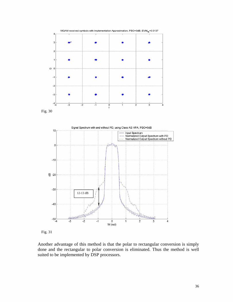
As the figures show, the squared amplitude and phase errors were reduced by more than 30 dB after about 200 samples. Fast convergence, Sufficiently small error in amplitude and phase, small enough EVM, about 15 dB reduction in Inter Modulation (IM) level can be obtained, close to saturation point, by a 32-entry Look up Table and reasonable complexity.

Fig. 29

36

Another advantage of this method is that the polar to rectangular conversion is simply done and the rectangular to polar conversion is eliminated. Thus the method is well suited to be implemented by DSP processors.

Fig. 30

Fig. 31

12-13 dB

37

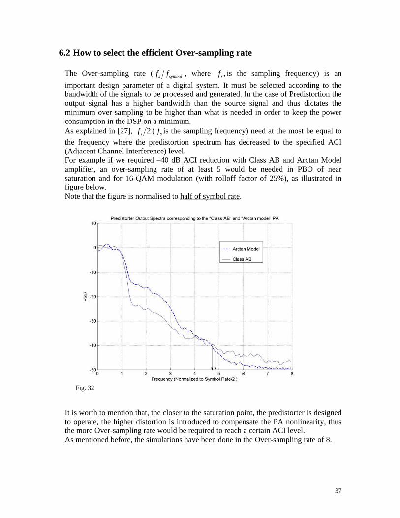
6.2 How to select the efficient Over-sampling rate

The Over-sampling rate ( symbols ff , where ,sf is the sampling frequency) is an important design parameter of a digital system. It must be selected according to the bandwidth of the signals to be processed and generated. In the case of Predistortion the output signal has a higher bandwidth than the source signal and thus dictates the minimum over-sampling to be higher than what is needed in order to keep the power consumption in the DSP on a minimum. As explained in [27], 2sf ( sf is the sampling frequency) need at the most be equal to the frequency where the predistortion spectrum has decreased to the specified ACI (Adjacent Channel Interference) level. For example if we required –40 dB ACI reduction with Class AB and Arctan Model amplifier, an over-sampling rate of at least 5 would be needed in PBO of near saturation and for 16-QAM modulation (with rolloff factor of 25%), as illustrated in figure below. Note that the figure is normalised to half of symbol rate.

It is worth to mention that, the closer to the saturation point, the predistorter is designed to operate, the higher distortion is introduced to compensate the PA nonlinearity, thus the more Over-sampling rate would be required to reach a certain ACI level. As mentioned before, the simulations have been done in the Over-sampling rate of 8.

Fig. 32

38

6.3 Effects of DAC and Reconstruction Filters on PD:

To obtain an ideal cancellation of the distortion and Intermodulation products caused by nonlinear amplifier, errors and memory effects must not be introduced between the Predistorter and the amplifier. The block diagram of predistortion linearizer is illustrated in figure 33. [27] A major source of memory effects is the reconstruction filters following the DA converters. One solution to reduce the impact of these filters is to use a high sampling rate reducing the demands on the filter and thus the memory effects introduced. However, as explained before, it is important that the sampling rate is kept as low as possible to obtain low power consumption in the DSP. The purpose of the reconstruction filter is to preserve the part of the spectrum located below 2sf carrying the distortion cancellation information and eliminate everything above this frequency, i.e. a lowpass filter. However any realistic filter approximation will contribute unwanted attenuation and phase shift below 2sf and thus introduces memory effects and degrades the distortion cancellation performance. The selection of filters may be confined to classical all-pole filters, namely Butterworth, Bessel, and Chebyshev. Maximum flat amplitude response in the passband is achieved by Butterworth, maximum flat group delay i.e. linear phase, by Bessel filters and steep slope by Chebyshev filters. As shown in [27], among these filters, Chebyshev filter with a small ripple and an order of 5 gives the best performance among others for Class AB and Class B power amplifiers.

DSP

Reconstruction Filters

I

Q

D/A

Quadrature Modulator

Fig. 33

39

7. DSP implementation and Experimental results

By now, we have talked about the different PD algorithms and some practical considerations and the Predistortion effects on spectrum and transmission quality were considered. The simulation results based on PA models were also shown. In this chapter, we will show an efficient way to implementation the non-adaptive predistorters in DSP and the experimental results are given with a real HPA.

7.1 Introduction to fixed-point DSP implementation

DSP processors use 2 different formats to save the data, namely, fixed point and float point formats (for some introduction in these formats, please refer to Appendix.D). In this case, fixed-point format is used to implement the Modulation, Filtering and Predistortion. Thus we tried to normalise the AM/AM and AM/PM characteristics of the amplifier to be suitable for fixed point programming. And as we will show in next section, this normalisation doesn’t introduce any effect on predistortion performance.

7.2 PA characteristic measurement and Predistortion Design

Figure 34 shows the configuration to measure the single-tone AM/AM and AM/PM characteristic of the amplifier. A 35dB Pre-Driver used to bias the amplifier near it’s saturation and a 30 dB attenuater used to derive the Network Analyser to avoid Network Analyser Overloading. The S-parameters were measured to find the gain characteristic (S [2,1]). The measured gain Characteristics for 27 dB dynamic rang as the input power for this Class AB HPA are shown in figures 35, 36.

Network Analyser

Pre-Driver 35 dB

HPAAttenuater 30 dB

Fig. 34

40

CH1 S21 LOG 1 dB/ REF 30 dB

START -45.0 dBm STOP -18.0 dBmCW 1 643 . 500 000 MHz

C

PRm

18 Nov 2003 14:16:22

1

1 : 30 . 500 dB -26.1 dBm

CH2 S21 PHA 5 / REF 165

START -45.0 dBm STOP -18.0 dBmCW 1 643 . 500 000 MHz

C

PRm

18 Nov 2003 14:16:16

1

1 : 169 . 34 -26.1 dBm

Phase Shift (degree) REF

Input Power dB

Input Power dB

REF Gain dB

Fig. 35

Fig. 36

41

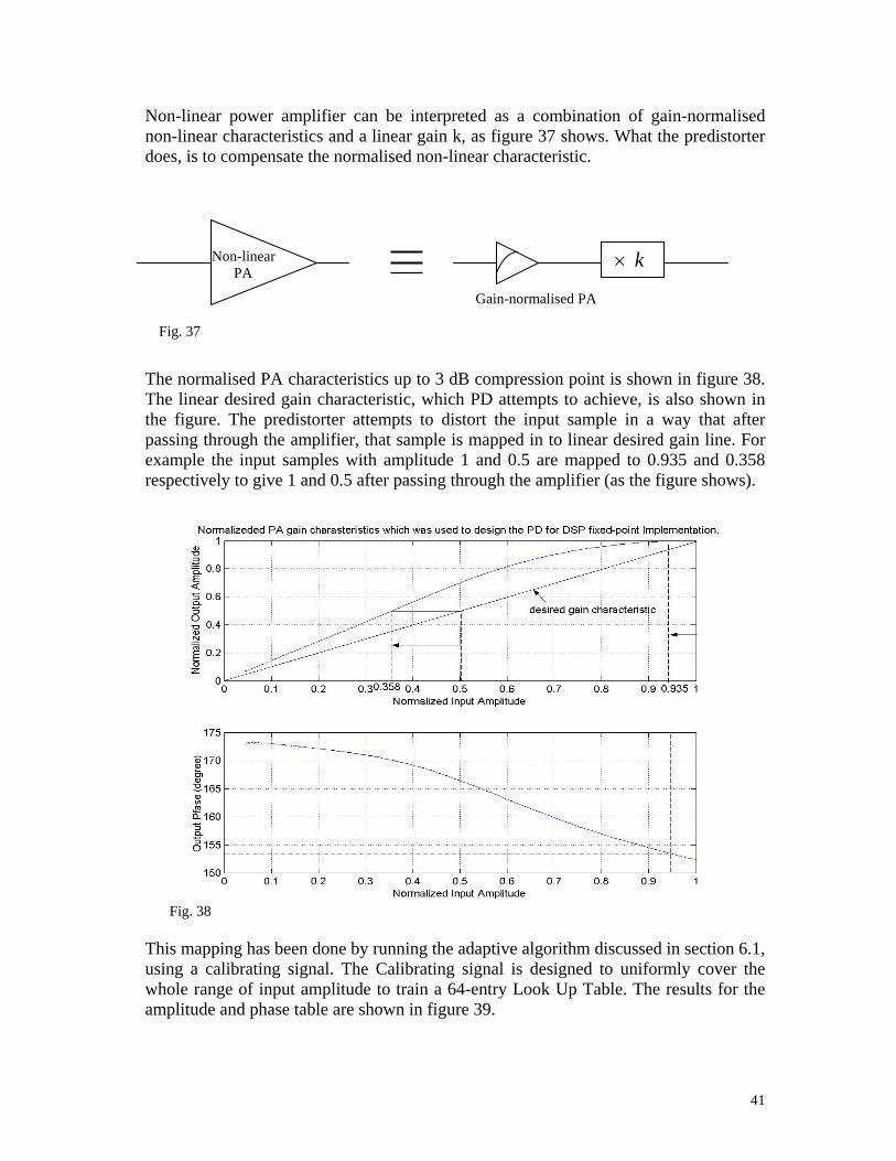
Non-linear power amplifier can be interpreted as a combination of gain-normalised non-linear characteristics and a linear gain k, as figure 37 shows. What the predistorter does, is to compensate the normalised non-linear characteristic. The normalised PA characteristics up to 3 dB compression point is shown in figure 38. The linear desired gain characteristic, which PD attempts to achieve, is also shown in the figure. The predistorter attempts to distort the input sample in a way that after passing through the amplifier, that sample is mapped in to linear desired gain line. For example the input samples with amplitude 1 and 0.5 are mapped to 0.935 and 0.358 respectively to give 1 and 0.5 after passing through the amplifier (as the figure shows).

This mapping has been done by running the adaptive algorithm discussed in section 6.1, using a calibrating signal. The Calibrating signal is designed to uniformly cover the whole range of input amplitude to train a 64-entry Look Up Table. The results for the amplitude and phase table are shown in figure 39.

Fig. 38

Non-linear PA

Gain-normalised PA

k×

Fig. 37

42

In this case we used the input Power (instead of amplitude) to access the table index (as figure 40 shows). Since we used uniform steps for the power-based table, the input amplitude isn’t uniformly reached. This may also introduce some degradation, however with this method the Square Root finding problem can be skipped. The PD, PA and Overall gain characteristic, obtained by actual 16-QAM samples is shown in figure 41. It can be seen that the desired linear amplitude characteristic has been obtained.

2

Pin I Q

Look up Table

nx ny

nknkn jQId ,, +=

Fig. 39

Fig. 40

43

7.3 Experimental Results

The platform that was used to accomplish the system is shown in figure 42 [29]. Symbol generation, Root Raised Cosine (RRC) pulse shaping [29] and predistortion were implemented by DSP Processor, ANALOG DEVICE 2181. A long FIR filter

DSP (Modulation, Filtering and Predistortion)

I

Q

DAC

Variable gain linear deriver

HPA Level Measurement and Spectrum Analysis

090

OSC

Fig. 41

Fig. 42

44

(128-tap) with an over-sampling rate of 8 is used to improve the performance and eliminate the memory effects due to filtering and 25% rolloff factor is proposed. Then the digital I and Q samples are converted in to Analog and passed through Quadrature Modulator at the center frequency of 1.6435 GHz. Since the RF level in the output of Quadrature Modulator is not high enough to drive the amplifier close to saturation, a 35 dB pre-driver is inserted to do that. It is worth to mention that the pre-driver was chosen to be highly linear, nevertheless still some nonlinearity was observed in its characteristics. However, since we measured the whole system characteristic with Network Analyzer, this nonlinearity has also been taken into account in the predistorter designing and the predistorter is designed to linearize the whole system. Thus the Pre-driver doesn’t introduce any effect in predistortion performance. Finally the measured Class AB 25dB-HPA used for this platform to evaluate the performance of Predistorter. The results observed by the Spectrum Analyser show about 15-20 dB reduction in adjacent channel emitted power. Figure 43 and 44 show the output spectrum of 16-QAM amplified signal without and with PD respectively. These results are based on the optimum output power up to about 3dB-compression point. Of course the performance degrades when we go further from this point, since it is a static algorithm and the PD designed up to a particular point of the amplifier gain characteristic and also the performance degrades with PA characteristic changes. Indeed (much) better performance and stability would be obtained with adaptive algorithms.

45

Fig. 43: 16-QAM Output Spectra without Predistorter

46

Fig. 44: 16-QAM Output Spectra with Digital Predistorter, about 17 dB reduction in Adjacent Channel Power Ration obtained with a 64-entry Table Lookup PD.

47

8. Conclusion

In this thesis, we investigated on Power Amplifier model and its effects on communication quality. Some algorithms are introduced to compensate for the non-linear characteristics of the amplifier. The performance of three different algorithms based on typical PA models were compared by simulations. The advantages and drawbacks were commented. Some practical considerations were made to improve the performance of predistortion. Finally a static look-up-table PD based on input power was implemented. As the results showed, predistortion, which has been introduced as a potential solution to improve the performance of amplifiers is able to linearize the amplifier up to points close to saturation. Further work will be to implement the adaptive algorithm, which requires designing the feedback path to find the error and feed the algorithm to update the predistorter.

48

References

[1] A.A.M.saleh, ‘frequency-independent and frequency-dependent nonlinear models of TWT amplifiers’, IEEE trans. Commun., Vol. Com-29, pp.1715-1720, Nov.1981. [2] S.Bendetto and E.Biglieri, ’Principle of Digital Transmission with Wireless Applications’, NewYork Kluwer Academic/Plenum Publishers, 1999. [3] S.C. Cripps, ‘RF power amplifiers for Wireless Communications.’ Norwood, MA:Artech House, 1999. [4] J.K.Cavers, ‘Amplifier Linearization Using a Digital Pre distortion with Fast Adaptation and Low Memory Requirements’, IEEE trans. on Vehicular Tech., Vol. 39, Nov. 1990. [5] M.Faulkner and Mats Johansson, ‘Adaptive Linearization Using Predistortion, Experimental Results’, IEEE trans. on Vehicular Tech. Vol. 43, No 2, May 1994. [6] H.Bebes, T.Le-Ngoc, ’A Fast Adaptive Predistorter for Nonlinearly Amplified M_QAM Signals’,0-7803-6451-1/00/$10.00, IEEE 2000 [7] Shawn P.Stapleton and Flaviu C. Costescu, ‘An Adaptive Predistorter for a Power Amplifier Based on Adjacent Channel Emissions’, IEEE Transactions on Vehicular Technology, Vol. 41, No.1, Feb. 1992 [8] M.Ghaderi, S.Kumar, and D.E.Dodds, ‘Fast adaptive polynomial I and Q predistorter with global optimization ‘, IEE Proc. Commun., Vol. 143, No 2, pp.78-86, April 1996. [9] Raviv Raich, Hua Qian and G.Tong Zhou, ‘Orthogonal Polynomials for Power Amplifier Modeling and Predistorter Design’, submitted to IEEE trans. on Vehicular Tech., Jan 2003 [10] Pierre R. Cheviliat and G. Ungerboeck, ‘Optimum FIR Transmitter and Receiver Filters for Data Transmission over Band-Limited Channels’, IEEE Transactions on Communications, Vol.Com-30, No. 8, Aug 1982. [11] J. K. Cavers, ‘Optimum Table Spacing in Predistorting Amplifier Linearizers’, IEEE trans. on Vehicular Technology, Vol. 48, No.5, Sep 1999 [12] J de Mingo and A.Valdovinos, ‘Performance of a new Digital Baseband Predistorter using Calibration Memory.’, IEEE trans. on Vehicular Technology Vol 50, No. 4, July 2001

49

[13] Inmarsat’s BGAN SDM, Vol.5, Ch.1, “UT Technical Requirement Specification”, Rev.2.1, 28 February 2003. [14] John G.Prokis ‘Digital Communications’. McGraw-Hill International edition 1995. pp. 278-281. [15] Derek S. Hilborn, Shawn P. Stapleton, James K.Cavers, ’An Adaptive Direct Conversion Transmitter’, IEEE Transactions on Vehicular Tech., Vol. 43, No.2, May 1994. [16] Andrew S. Wright and Willem G. Durtler, ’Experimental Performance of an Adaptive Digital Linearized Power Amplifier’, IEEE Transactions on Vehicular Tech. Vol. 41, No. 4, Nov 1992. [17] Aldo N. Andrea, Vincenzo Lottici and Ruggero Reggiannini, ‘RF Power Amplifier Linearization through Amplitude and Phase Predistortion’, IEEE Transactions on Communications, Vol. 44, No. 11, Nov 1996. [18] G. Tong Zhou and J. Stevenson Kenney, ‘Predicting Spectral Regrowth of Nonlinear Power Amplifiers’ IEEE Transactions on Communications, Vol. 50, No. 5, May 2002. [19] Dong Seog Han and Taewon Hwabg, ‘An Adaptive Predistorter for the Compensation of HPA Nonlinearity’, IEEE Transactions on Broadcasting, Vol. 46, No.2, June 2000. [20] ADSP-2100 Family Reference Manual, 1995 ANALOG DEVICES. [21] ADSP-2100 Family User’s Manual, 1995 ANALOG DEVICES. [22] J.Kim and K.Konstantinou, ‘Digital Predistortion of Wideband Signals based on Power Amplifier model with Memory’, Electronic Letters, Vol. 37, No. 23, 8th Nov. 2001. [23] Changsoo Eun and Edward J. Powers, ‘A New Volterra Predistorter Based on the Indirect Learning Architecture’, IEEE Transactions on Signal Processing, Vol. 45, No.1, Jan 1997. [24] Giovanni Lazzarin, Silvano Pupolin, Augusto Sarti, ‘Nonlinearity Compensation in Digital Radio Systems’, IEEE Transactions on Communications, Vol. 42, No. 2/3/4, Feb./March/April 1994.

50

[25] ‘Analysis, Measurement and Cancellation of the BandWidth and Amplitude dependence of Intermodulation Distortion in RF power Amplifier’, PhD Thesis, University of Oulu in Finland. http://herkules.oulu.fi/isbn9514265149/html/index.html [26] Bassam Hashem and Mohamed Samy El-Hennawey, ‘Performance of the

,4 DQPSK−π GMSK and QAM Modulation Schemes in Mobil Radio with Multipath Fading and Nonlinearities’, IEEE Transactions on Vehicular Tech. Vol. 46, No. 2, May 1997. [27] Lars Sundstrom, Michael Faulkner and Mats Johansson, ‘Effects of Reconstruction Filters in Digital Predistortion Lineariaers for RF Power Amplifiers’, IEEE Transactions on Vehicular Tech., Vol. 44, No. 1, February 1995. [28] James K. Cavers, ‘The effect of Quadrature Modulator and Demodulator Errors on Adaptive Digital Predistorter for Amplifier Linearization’, IEEE Transactions on Vehicular Tech. Vol. 46, No. 2, May 1997.

51

APPENDIX A AM/AM and AM/PM characteristics of different amplifiers, obtained based on 1-tone measurements are shown below.

52

APPENDIX B In the Inmarsat specification, and in the Cobra Requirement Specification document, 2EVM [%], i.e. [ ]

22% 100 linEVMEVM ⋅= , is specified.

Another possible 2EVM definition is based on the outmost symbols in the modulation constellation, i.e.

( )2

1

0

22

2

1

peak

N

jjj

peak S

QIN

EVM∑−

=

+

=

δδ

For 16-QAM, 22 8.1 meanpeak SS ⋅= . Hence 22 8.1 peaklin EVMEVM ⋅= , and [ ]22

% 180 peakEVMEVM ⋅= .

The relationship between 0NEs ( sE : Energy per symbol, 0N : Power-Spectrum-Density (PSD) of Additive-White Gaussian-Noise (AWGN)) and 2EVM [%] can be shown to be

[ ] ( ) [ ]( ) ( )peaklindBs EVMEVMEVMNE 10

2%10

2100 log2055.2log1020log10 −−=−==−=

53

where 2peakpeak EVMEVM = . Hence, [ ] %12

% =EVM corresponds to =0NEs 20dB and

[ ] %3.02% =EVM corresponds to =0NEs 25.2dB.

APPENDIX C

The theoretical calculation of probability of making an error in M_QAM modulations in AWGN channel and for even k=log2(M) is given as [14]:

⎟⎟⎠

⎞⎜⎜⎝

⎛

−⎟⎠⎞

⎜⎝⎛ −=

0

,2

1log3112

NE

MMQ

Mp aveb

M

( )2, 11 MSyme pP −−= .

Symebite PM

P ,2

, log1

≈ with Gray coding.

Note that in MATLAB Q function can be built as:

⎟⎠⎞

⎜⎝⎛−=

221

21)( xerfxQ .

APPENDIX D

Discussion on Data Formats in DSP processors: DSP processors store data in fixed or floating point formats. It is worth noting that fixed point format is not quite the same as integer: Integer (e.g.):

0 1 0 1 0 0 1 1 72− 62 52 42 32 22 12 02 = 832222 0146 =+++ Fixed point (e.g.):

54

0 1 0 1 0 0 1 1

02− 12− 22− 32− 42− 52− 62− 72− = 64843.02222 7631 =+++ −−−−

The integer format is straightforward: representing whole numbers from 0 up to the largest whole number that can be represented with the available number of bits. Fixed-point format is used to represent numbers that lie between 0 and 1: with a 'binary point' assumed to lie just after the most significant bit. The most significant bit in both cases carries the sign of the number. The size of the fraction represented by the smallest bit is the precision of the fixed-point format. The size of the largest number that can be represented in the available word length is the dynamic range of the fixed-point format. As an example, for the 8-bit format shown above, the precision is 0078125.02 7 =− and the dynamic range is [-1,1- 72 ], thus 0xFF is the smallest and 0x7F is the largest number in hexadecimal format.

To make the best use of the full available word length in the fixed-point format, the programmer has to make some decisions: If a fixed point number becomes too large for the available word length, the programmer has to scale the number down, by shifting it to the right: in the process lower bits may drop off the end and be lost If a fixed-point number is small, the number of bits actually used to represent it is small. The programmer may decide to scale the number up, in order to use more of the available word length

In both cases the programmer has to keep a track of by how much the binary point has been shifted, in order to restore all numbers to the same scale at some later stage. Floating point format has the remarkable property of automatically scaling all numbers by moving, and keeping track of, the binary point so that all numbers use the full word length available but never overflow: Mantissa

0 1 1 0 1 0 0 1 1 12−− 02 , 12− 22− 32− 42− 52− 62− 72−

mantissa = 64843.122222 76310 =++++ −−−−

Exponent 0 1 1 0

32− 22 12 02 exponent = 622 12 =+ decimal value = 49952.105264843.1 6 =×

55

Floating point numbers have two parts: the mantissa, which is similar to the fixed point part of the number, and an exponent which is used to keep track of how the binary point is shifted. Every number is scaled by the floating-point hardware: If a number becomes too large for the available word length, the hardware automatically scales it down, by shifting it to the right If a number is small, the hardware automatically scale it up, in order to use the full available word length of the mantissa In both cases the exponent is used to count how many times the number has been shifted.

56

List of Programs M-QAM Symbol generation and Root Raised Cosine Filtering: (Written by Biarne Rislow, Nera Research) • M_QAMgen.m • sqrtrc.m • zerofill.m PA model: • HPA_model.m : HPA Model based on measurement • Poly_model_amp.m : Arctan Model • amp_model.cpp Look Up Table Adaptive PD: • LUT_2_Updating.m • VarSiz_LUT_mod.m • table_setting.m Parametric Adaptive PD: • Parametric_PD.m Hybrid Adaptive PD: • LUT_POLY.m Bit Error Rate Performance and Spectrum Estimation: • Pe_sim_withoutPD.m • Pe_sim_withPD.m • Q_fun.m • Pe_Sim.cpp • plot_spectrum.m Adaptive PD with Implementation Consideration: • efficient_LUT_mex.m • efficientLUT.cpp • Implementation_LUT.m Matlab Programs used for fixed-point DSP Implementation: • fixed_point_LUT.m • Predistorted_data_PA.m DSP Projects (Symbol Generations, Interrupt Service routines and Filtering, written by Knut Rimstad, Nera Research): • transmitter_QPSK Folder: includes <.dat>, <.asm> and <.ldf> files • transmitter_16QAM Folder: includes <.dat>, <.asm> and <.ldf> files • FeedBack_Line Folder: includes <.asm> and <.ldf> files