Purdue University Purdue University

Purdue e-Pubs Purdue e-Pubs

Department of Electrical and Computer Engineering Technical Reports

Department of Electrical and Computer Engineering

May 1993

ADAPTIVE CONTROL OF REDUNDANT MULTIPLE ROBOTS IN ADAPTIVE CONTROL OF REDUNDANT MULTIPLE ROBOTS IN

COOPERATIVE MOTION COOPERATIVE MOTION

Mohamed Zribi Purdue University School of Electrical Engineering

Shaheen Ahmad Purdue University School of Electrical Engineering

Shengwu Luo Purdue University School of Electrical Engineering

Follow this and additional works at: https://docs.lib.purdue.edu/ecetr

Zribi, Mohamed; Ahmad, Shaheen; and Luo, Shengwu, "ADAPTIVE CONTROL OF REDUNDANT MULTIPLE ROBOTS IN COOPERATIVE MOTION" (1993). Department of Electrical and Computer Engineering Technical Reports. Paper 229. https://docs.lib.purdue.edu/ecetr/229

This document has been made available through Purdue e-Pubs, a service of the Purdue University Libraries. Please contact epubs@purdue.edu for additional information.

TR-EE 93-19 MAY 1993

ADAPTIVE CONTROL OF REDUNDANT MULTIPLE ROBOTS IN COOPERATIVE MOTION

Mohamed Zribi, Shaheen Ahmad and Shengwu Luo

Real-time Robot Control Laboratory School of Electrical Engineering Purdue University West Lafayette, IN 47907-1285 U.S.A

ABSTRACT

A redundant robot has more degrees of freedom than what is needed to uniquely position the robot end-effector. In practical applications the extra degrees of fieedom increase the orientation and reach of the robot. The load carrying capacity of a single robot can be increased by cooperative manipulation of the load by two or more robots. In this paper we develop an adaptive control scheme for kinematically redun- dant multiple robots in cooperative motion.

In a usual robotic task, only the end-effector position trajectory is specified The joint position trajectory will therefore be unknown, for a redundant multirobot system and it must be selected from a self-motion manifold for a specified end-effector or load motion. We show that the adaptive conuol of cooperative multiple redundant robots can be addressed as a reference velocity tracking problem in the joint space. A stable adaptive velocity control law is derived it ensures bounded parameter conver- gence, exponential convergence to zero of the load position error, the internal force error and the reference velocity error. The individual robot joint motions is shown to be stable by decomposing the joint coordinates into two variables one which is homeomorphic to the load coordinated, the other to the coordinates of the self-motion manifold. The dynamics on the self-motion manifold is directly shown to be related to the concept of zero-dynamics. It is shown that if the reference joint trajectory is selected to optimize a certain type of objective functions, then stable dynamics on the self-motion manifold results. The overall stability of the joint angle is established from the stability of two cascaded dynamic systems involving the two decomposed co0rdlIliltes.

1. INTRODUCTION

Recently considerable amount of research has focused on the problem of cooperative control and coordination of multiple robots. Interest in multi-robot sys- tems has arisen because several tasks require the use of two or more robots. Examples of such tasks include the joining and securing of large pipes for the construction of space structures, picking up and carrying heavy loads, and grasping odd shaped loads. Cooperative robots may be used in hazardous or unsafe environments such as in space, in deep waters and in radioactive environments. By using more than one robot the manipulation capability and the workspace of the system may be further increased However cooperative multiple-robot systems are more difficult to control than single robots. Additional problems may arise in the control if the parameters of the robots and the manipulated load may not be known exactly.

Several control schemes, adaptive and non adaptive schemes have been pro- posed for cooperative multiple robots with rigid joints manipulating a common load. Zheng and Luh [32] considered the kinematic and dynamic model of the multi-robot system and developed an inverse dynamics schemes for load position control. Hsu et al 1231 developed a control algorithm for the coordinated manipulation of multi- fingered robot hands. Tarn, et al [28] developed a robust nonlinear control scheme using nonlinear transformation techniques. Yun, et a1 [29] also used exact lineariza- tion and output decoupling techniques to control multiple robots. Yoshikawa and Zheng [31] also developed linearizing tracking control laws for multiple robots, experiments were also reported. Few adaptive control schemes for cooperative robots manipulating a common load have been proposed. Walker et al. [30] developed an adaptive algorithm for the control of two robots handling a common load of an unknown mass. Zribi and Ahmad [24] proposed a robust adaptive con- troller for the multi-robot system manipulating a rigid object cooperatively when sub- ject to bounded disturbances. The problem of manipulating a load using multiple robots when the load makes contact with an environment was addressed by Hyati [33], Cole [34] and, Hu and Goldenberg [27]. Ahmad and Guo [26] addressed the problem of controlling multiple flexible-joint robots with linear dynamics. Ahmad 1351 developed a feedback linearizing controller for multiple flexible joint robots.

There are a very few papers in the area of control of multiple redundant robots, these include the recent paper by Tarn et al. [36] which addressed the zero dynamics issue. The paper by Tao and Luh [37] also addressed multiple redundant robot con- trol. The reason there is such a few works in the multiple redundant robot control is primarily because non-redundant robot control schemes cannot be easily extended to control redundant robot systems. This is because a redundant robot has more joints than what is required to position the end-effector. Usually the end-effector trajectory

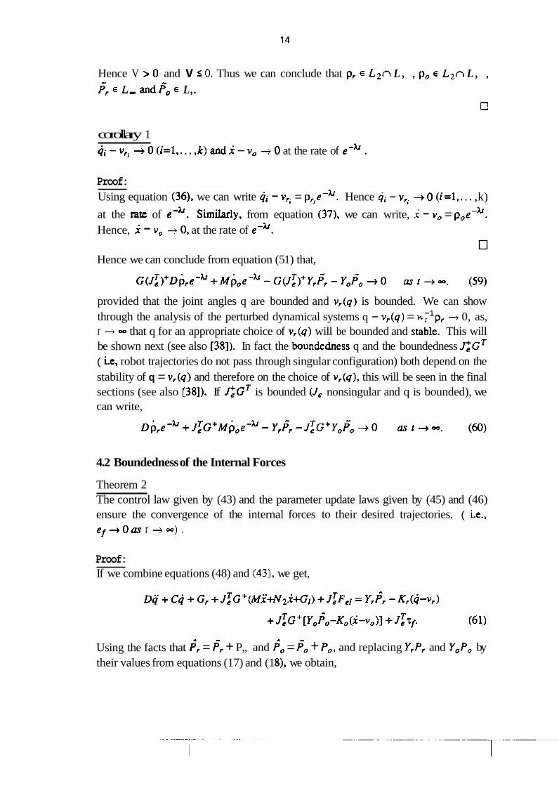
is known and thus the joint trajectory cannot be found uniquely. In fact, for a fixed end effector position there is a self-motion manifold on which joint motions could occur without effecting the end-effector position. In Figure. 1, we show a planar redundant robot with three prismatic axes, we see if the end-effector is stationary the joints may move in a straight line in the joint space without effecting the end- effector. Any arbitrary joint trajectory which ensures end effector position cannot be used as this may not result in stable joint motions on the self motion manifold and would therefore effect overall stability. These two problems have prevented the sim- ple extension of non-redundant strategies being adopted for multiple redundant robots. We should note here that the extra joints are extremely useful in real applica- tions as they can be used to configure the manipulator posture, to avoid obstacles in the workspace or to avoid joint singularities.

Initial interest in the control of redundant robots started with the work of Whit- ney [21] who devised a kinematical resolved motion rate control strategy. Since then a number of researchers have addressed the the joint coordination and control of redundant robots (see Nenchev [13] for a review of those developments). The tutorial review by Siciliano [17] and the tutorial workshop report on the theory and application of redundant robots at the 1989 IEEE robotics and automation conference ['I] covered some more recent developments (see also [ 1-3,7,11- 14,16,17]). In the area of redundant robot adaptive control, Seraji [16] presented an approach based on the model reference adaptive control theory. He resolved the redundancy problem by adding additional task dependent kinematic constraints to the end-effector kinemat- ics. This effectively ensured the joint solutions were unique. Niemeyer and Slotine [14] applied sliding mode adaptive control to redundant manipulators. They used the passivity principle to prove the stability of the adaptive system. Niemeyer and Slotine also performed some experiments to demonstrate their control law. Colbaugh et al. [3] proposed an adaptive inverse kinematics algorithm that did not require the knowledge of the kinematics of the robots. However their algorithm required per- sistent excitation conditions; also their algorithm did not consider the dynamics of the robot. Luo, Ahmad and Zribi [38] developed an adaptive control law for redundant robots making use of weighted scaling functions and the concept of zero dynamics to show both the joint motions on the self motion manifold and the end-effector motions would be stable for their control law.

In this paper, we address the problem of controlling redundant multiple robots manipulating a load cooperatively. We assume the load mass/inertial parameters and the robot joints masfinertial parameters are unknown. We first state the dynamic models of the robots and the load and give a few properties of the multi-robot system. Next the redundancy ~lesolution problem is discussed, and a model for adaptive reso- lution of the redundancy is established. A controller that leads to the exponential tracking of the load position and the convergence of the internal forces to their desired values is then derived. The boundedness of the joint motion and control torques are proved next. The conclusions can be found in the final section of the

paper.

2. MULTI-ROBOT SYSTEM MODEL

2.1 Dynamics Model

The general dynamic model for a cooperative multi-robot system has been investigated thoroughly in the literature, and is also described in the below for com- pleteness. In Figure. 2 we depict the organization of the multiple robots grasping a common load which is to be manipulated cooperatively. We first state a few assump- tions related to the robots grasp of the load and the reachability of the trajectory that will be used in the subsequent derivation. Assumptions (Al) The manipulators are rigidly grasping the load, (i.e., there is no motion between the contact point of the load and the robots end-effectors). (A2) The desired trajectory is reachable and the end effector can be positioned at those workspace (of dimension six) positions without exceeding any joint motion limits.

The dynamic equation of the ith manipulator in cooperative manipulation can be written as,

Di(qi)ii + Ci(qi,Qi)4i + Gi(qi) + J~~ ( q i ) T ~ e i = i=l,. . . ,k. (1)

where, qi E R4 is the vector of joint displacements, and ni>6 is the number of joints of the ith robot The inertia matrix of the ith robot is Di(qi) E R nix', this is a positive &finite and symmetric matrix. The matrix of centrifugal and Coriolis forces is

Ci(qi7Qi) E R4%; the vector of gravity forces is Gi(qi) E Rni, and the manipulator Jacobian is J, (4,) E R -. The control input torque for the ith robot is g E R &. We

i =k will &fine the total number of joints of the k robots as n, n = Cni .

i=l

The forces/moments applied by the ith manipulator on to the object at the point of contact are Fei. The contact forces/moments Fei E R6 can be written in terms of

the contact forces fei E R~ and contact moments qei E R3, (when 6 represents the

dimension of the Cartesian work space), such that,

Now we will group the dynamics of the k-robots system to get,

where D E Rn'"' is a block diagonal matrix whose diagonal elements are Di E Rnixn,. C E R"'"' is a block diagonal matrix whose diagonal elements are Ci E R

niXni and J E R6k" is a block diagonal matrix whose diagonal elements are Jei E RbXni. Also

we will define the following vectors as, T T T T T q=[q lT . . . q k T ] T , ~ r = [ ~ l T . . . Gk ] , T = [ T ~ ... ~k ] and, Fe=[F:, ... FebT]f4)

If we assume that the object is rigidly grasped, then the equations of motion of the object are obtained from the Newton-Euler mechanics as,

where the position of the center of mass of the object expressed in the world coordi- nate frame is xp E R3 . The rotational velocity of the object expressed in the world coordinate M e is o E R3, and the gravity force vector of the object, expressed in the world coordinate reference frame is gr E R3. The mass matrix M 1 E R 3x3 is a diagonal mamx whose diagonal elements are the mass of the load; the matrix I E RW is the inertia matrix of the load. The vector ri = [rk,riY,rklT e R3 represents the translational displacements from the center of mass of the object to the contact point of the object and the ith manipulator.

. T If we let x = [ x, d lT, then the motion of the object expressed by equation

(5) and (6) can be written as,

where G E R66k is the grasp mamx; G is defined as,

G = [TI TZ ... Tk] . (8)

The mamx Ti E R~ is such,

and , Ri(ri) =

The mamx 13x3 E R~~~ is the identity mamx. Also we have,

M1 0 M = [0 I], Ni= [ O ] and GI= [M;gl]. ~ ( I w )

2.2 Kinematic Model

We are interested in controlling the manipulators in some predefined Cartesian task space such that,

where Kei(.) : R'*+R6 is the transformation from the joint angle space of qi to the

task space containing Xei, and xei E R is the position and orientation of the point of

contact of the ith manipulator, with the load, expressed in the world coordinate frame. If we differentiate equation (10) with respect to time, and if we define ,Jei(qi) to be the

differential map from the qi space to xei space, then we can write,

If these equations are stacked into a single vector by forming the Jei into a block

diagonal matrix, and concatenating the qi 's into one vector q, we get,

. T .T T where vc = [ic, x,, . . . xeb] is the velocity vector at the contact points and

J, = diag (J, , , . . . , Jem ).

Using equation (7), we can write,

F, = GF,

Now from the duality between the forces and the velocities, we can write,

T G x = v c , (14)

where x is the velocity of the object. Thus for the k robots system, we can combine equations (12) and (14) to get,

cTx = ~~q . where G is the grasp matrix defined earlier.

2 3 Definition of Internal Forces and Internal Force Errors

The end-effector force of the ith manipulator, Fei, can be decomposed into two forces, the motion force and the internal grasping force. The internal grasping forces Fl = [ F l e ~ , . . , ~ I e k ] T ~ ~ 6 k do not cause any motion of the load. However we must control these end-effector internal forces, F ~ ~ ~ E R ~ with i=l. ... k, in order to prevent excessive compressive or expansive forces being applied to the load. 'We can calcu- late the internal force FI from equation (7) if F, is known and rank (G )= 6, then

Here, G+=GT(GGT)-' and GG+=16, given I 6 is an 6x6 identity matrix. (For a dis- cussion related to other choices of the inverse of the G+ matrix see [36] and [39]. Notice that other choices of the inverse of G does not effect the derivations presented in this paper.) Therefore we see that GFI=O and GFe=Fo, i.e, the internal forces do not contribute to the motion of the load. The desired internal forces F ~ , ~ E R " also satisfy GFlnd=O. The internal force error, ef = F I , ~ - FI, also satisfies

These internal force properties will be used to derive the control law.

2.4 A Few Properties of the Multi-Robot System

In the following we will state several properties which will be used in the derivations of the controller. S ys tem Dynamics Properties (Pl) D and M are symmetric positive &finite matrices. -

1 1. (P2) D - 2C is skew symmetric mamx or - q (D -2C)q =O . The proof of property

2 P2 can be found in 1191 and [ a ] .

1 -7- (P3) M - 2 N z is skew symmemc mamx or, x (M -2N)x =O . This property can

be seen from energy considerations. In general if M is not expressed in the object center of mass coordinate frame, M=M (x) and Nx=N(x,x)li. The total energy of the

1 .T load is given by EL=T x Mx + h(x) where h(x) is the potential energy and - d GI=- h(x). As the power input to the load is given by, ax

d .T .T 1 . T -EL=x F o a (Mi + - M i +Gl)=x (Mi + Ni + GI), thus we have the property, $ T 2

-i (ni-rn)li=o. 2

Two important properties of the inertia matrix, the cenmfugal/Coriolis mamx and the gravity vector which will be used in the developments are now given.

(P4) Linear Parameterization of the Robot Dynamics

The linearity of D, C and G, with respect to the manipulators dynamic parame- ters P, E RS1 is now stated, these parameters will be estimated by the proposed adap- tive scheme. The robot dynamics can be linearly parameterized [19], [40] and,

Da, + Cv, + G, = Y, P, , (17)

where a, E R n and v, E R n are vectors and we denote a, as the "reference accelera- tion of the robots" and also, v, is the " reference velocity of the robots." The regres- sor matrix Y,(q,q,v,,o,) E RnW' represents the structure of the robots dynamics, hence its elements are combinations of the nonlinear functions present in the inertia mamx, cenmfugaVCoriolis matrix and the gravity vector.

(P5) Linear Parameterization of the Object Dynamics

The second property deals with the linearity of M, N2 and GI with respect to the load parameter vector Po,

Ma, +N2vO +GI =YoPo (18)

where a, E R6 and vo E R6 are the "reference acceleration of the load and the "reference velocity of the load," respectively. We will denote by Po E RS" the vector of so load parameters which are constants for a given load. These parameters will be estimated by the proposed adaptive scheme. The regressor matrix Y,(x,x,v,,a,) E RrrY. represents the structure of the load dynamics.

Remark 1

Let i, be the vector of estimates of the parameters of the robots, then the error

vector in the estimates of the robots parameters is Fr = Gr - P, . Similarly, we can

write the parameter estimation error vector for the load as Po = io - P , . Notice that we can write,

A n A n

Da, + Cv, + G, = Y,P, ,

where d is the estimate of the inertia mamx D, C ̂ is the estimate of the

Coriolidcenmfugal mamx and 6, is the estimate of the the gravity vector. Also notice that, fia, + C?vr + 6 = YrPr = Y,($, - P,) , where 6 is the e m r in the inertia

mamx, E is the e m r in the Coriolislcenmfugal mamx and 6, is the error in the grav- ity vector.

Similarly we can write, A A A A

Ma, + N2v0 + GI = YoPo , (20)

where M is the estimate of M, hi2 is the estimate of N2 and el is the estimate of GI.

Also notice that MU, + c2v0 + 6! = YoF0, where i, i2 and el are the differences between the estimates and the true values.

3. REDUNDANCY RESOLUTION PROBLEM

3.1 Preliminaries

Consider a kinematically redundant manipulator with the camed load center of mass positioned at point x, and the joint position qi. Then the differentiable kinematic mapping is Ki such that,

where x E R ti is the position of the load and qi E R~ is the vector of joint positions of the ith manipulators and as ni > 6, the degree of redundancy of the ith robot is r; = ni - 6. As a result of the joint redundancy at the end effector point x = xd, there will exist a set of joint angles, the self motion manifold such that Qgi = {qi I x = xd = Ki(q)}. (Recall the example in Figure. 1, the self motion mani-

fold was the line in the joint space.) Thus, in order to find a unique joint angle q, additional requirements are necessary; these will be stated later. We will denote the Jacobian of the kinematic map (21) by, Ji = T;~J, E R6xni. This relates differential

map between the load position kinematics Ki(*) and the end effector kinematics &(a). The projection operator onto the null space of Ji is denoted by

PJi(qi) (i=l,. . . ,k). Also let all the columns of matrix NJi be the basis of ker (Ji),

which is the null space of Ji. Hence we have,

JiPJi = 0, and ker (Ji ) = span (Nji ). (22)

The matrix NJi E RhVi has the following properties that will be used in the text,

T + = O E R'ix6 JiNJi = 0 E R 69 NJ J: = 0 E R 'jX6 , N Ji 9 (23)

foranyvector 4 i € R 4 ~ ~ N ~ ~ ~ = O E R ' ' ' t h e n P ~ ~ 4 ~ = 0 ~ ~ * . (25

Notice also that [ J k ] is a square matrix of full rank, thus we have, NJ,

These properties show that the pairs (Ji,NX) and (c ,Nj i ) are orthogonal complement

operator pairs.

3 3 Statement of the Problem of the Redundancy Resolution

The redundancy is usually resolved by the constrained optimization of a perfor- mance index Hi (i =l,. . . ,k), this function can be used to avoid joint limits, obstacles and singularities (see the review papers listed in the reference). The problem can be formulated as follows: given a desired position xd, find the joint position qi ( i=l , ..,k) such that,

min Hi(qi) with xd = Ki(qi) i= l , . . . ,k . 4i

(27)

We can conclude from the Lagrange multiplier method that the solution of the con- strained optimization problem (27) necessarily satisfies the following set of con- strained diffe~lential equations:

PjiVHi(qi)=O and xd=Ki(qi) i=l,. . . ,k . (28)

We will define the end-effector path tracking error e as,

e =Ki(qi)-xd j=l, . . .,k. (29)

Our g o d is to resolve the "asymptotic resolution of the redundancy problem" such that as t + =, we have,

e +0, e + 0 , and, PjiVHi(qi) + 0 i=l,. . . ,k. (30)

We want to optimize Hi ( i=l,. . . ,k) by appropriate joint motion on the self-motion manifold, Q;Gi ( i =l,. . . , k). At the optimal point, we do not desire further motion on

the self motion manifold. Therefore the projection of the joint velocity on the self-

motion manifold must be zero, and ~ $ 4 ~ + 0 as, t + =. Thus it is sufficient (not

necessary) to write the asymptotic redundancy resolution as t-+=,

Here, y > 0 and pi f 0. The first equation can be written as Jiqi -;id +ye + 0 . After grouping terms and using the matrix inversion expressed by (26), we find qi, and, as t +-,

Therefore the "asymptotic resolution of redundancy problem" can be expressed by the conditions given by (32). These conditions result in the joint velocities approach- ing their desired values, while the joint positions satisfy a set of constmint equations. Notice that the redundancy resolution problem is characterized by the fact that the desired joint positions are not known in advance. This fact prevents us from directly using the existing adaptive schemes that achieves joint position tracking.

We will denote by vri (i=l,. . . ,k) the joint reference velocity for the ith robot.

We also will denote by vo the load reference velocity. We will choose v r i (i=l,. . . ,k)

such that,

We will group the v ( = l k ) into one vector vr such that, T vr = [vf, vr, . - . v; IT is the joint reference velocity of the robots. We will

L J

choose vo such that,

vo =xd -ye .

It should be noted that the choice of vo guarantees that,

v o = J i v , = ~ T ~ e i v r i i= l , ..., k.

The asymptotic resolution of redundancy problem can be solved by a mechanism that ensues qj - vri + 0, Cfor i =l, . . . ,k), as t + w.

In order to proceed further we will state a few more assumptions these will be needed in the control law development.

3.3 Assumptions - Continued

(A3) The desired paths xd(t), xd (t ) and fd(t) are bounded for all time t.

(A4) The Jacobian Ji(qi) (i =1, . . . , k) is a full rank continuously differentiable func- tion matrix, that is, Ji(qi) is of class Cr, r22. (i.e., at least twice differentiable).

(AS) The cost function Hi (qi) (i = 1,. . . , k) given in (27) is a twice differentiable real valued function.

In assumption (A4) the full rank restriction on Ji(qi) (i =l,. . . ,k) requires that all possible joint motions q;, do not pass through any singularity configuration of Ji(qi), this will be shown to be possible with the control law derived in this :paper, this will be addressed in the final section of the paper (see also [38]). If Ji(qi) is continuous and full rank in some subset GJi c R", then Jt = ~f (J~J~)-', Pji = I,-CJi and NJi

are continuous in GJi. The mamces Ji, J t , PJi and NJi are shift varying linear opera-

tors. It is easy to show that any continuous linear operator is bounded, hence Ji, J t , PJi and NJi are bounded in GJi, (i.e. the induced norm of Ji, J t , PJi and Nji are finite

a in GJ,). Furthermore, if ji is continuous in Gji , then - and PJi are continuous on

dt any path with continuous qi in GJi .

4. DESIGN OF THE CONTROL AND UPDATE LAWS

4.1 Design of the Control Law

Our goal is to design an adaptive controller that guarantees the asymptotic con- vergence of the load tracking enor to zero, the convergence of the internal forces to their desired values and the redundancy resolution. We will start by defining a few variables needed for the development. The weighted reference velocity error for the ith robot is defined as,

The scalar weighting function w, will be chosen as, w, = e b , where b is a positive constant (see [18] for the use of weighting functions in the adaptive control of single

rigid robots). We will group the p,, (i=l,. . . ,k) into one vector p, such that, T

P, = [PT~ PT, - . . PL] . Also the weighted reference velocity error for the load is

defined as,

It is easy to show that,

We will choose p, and p, such that,

p r i = ~ f ( 4 i - a r i ) i=l, ..., k ,

and, p, = w,(x -a,) . (40)

The choice of pri given by equation (36), and the choice of given by equation (39)

will result in the following value for a,. ,

We can group the a = l , . . . , k ) into one vector a, such that, T T

a, = FJ, a,, . . . a;] . The choice of po given by equation (37), and the choice

of given by equation (40) will result in the following value for a,,

Notice that v, and v, are in&pen&nt of q and i , hence a, and a, are not functions of

q and x. Therefore the proposed adaptive scheme does not require the measurements of 'the accelerations q and x.

Theorem 1 Given that the matrices KO, K,, I', and I', are positive definite mamces, Kf is a posi- tive semidefinite diagonal mamx, the control law given by (43) and the parameter update laws given by (45) and (46) ensure that p, , p, E L 2 n L, and that P, , Po€ L,.

T + ^ r =aa, + d ~ , + 6, -K,(~-v,) + J e G [Ma, +]S~VO + dl -Ko(i-vo)]+ J:rf

The force torque rf is given by,

T~ = F ~ ~ - ~ ~ j e l ,

The parameters update laws are such,

Preliminaries to the Proof.

Before proving theorem 1, we will derive the equation of the closed loop sys- tem. We can solve for the force from equation (7), thus we get,

If we combine equations (3) and (47), we get,

D+ + + G, + J:G+(MY + N 2 i + G ~ ) + JTF~I = 7 . (48)

Now we will multiply both sides of equation (48) by GUT)+ , we get,

G (J:)+[ Dq + Cq + G, ] + M i + N2x + GI = G(J:)+~ . (49)

Here we used the fact that GFd = 0. Replacing r by its value from equation (43), and using the fact that Gzf = 0. we get,

Replacing Y,P, and YoPo by their values from equations (17) and (6), we obtain,

G(J;)+[ D(*,) + c(4-vr) + K,(q-v,) ] + M(2 - a,) + N2(i-v,) + Ko(i-v,)

= G(J;)+Y,F, + yoFo . (5 1)

Thus the composite system can be written as,

G(J;)+[D~, + ~ p , +Kip,] + Mp, + N ~ P , +Kop0 = G(J~)+Y,F,.w, + Y,F,w,. (52)

Proof of Theorem 1 : Consider the following Lyapunov function candidate

Now if we differentiate V with respect to time and use propemes P1 - P3, we get,

~ = P ~ [ D ~ ~ + c ~ ~ I + ~ ~ ~ , F ~ + ~ : [ M ~ , + N ~ ~ , ] + F : ~ ~ , F , , (54)

using the fact that p, = G , v becomes,

Using equation (52), we get,

Using the update laws given by equations (45) and (46), we get,

Thus,

v=- ~ $ G ( J ~ ) + x ; J : G ~ P , - p z ~ o p o =- P;K,P, - P:K,P, . (58)

Hence V > 0 and v s 0. Thus we can conclude that p, E L 2 n L , , po E L 2 n L , , - F, E L , and^, E L,.

corollary 1 qi -v, + 0 (i=l,. . . ,k) a n d i -v, + 0 at the rate of e-h .

Proof: Using equation (36), we can write qi - vri = p,e-h. Hence ii - v, + 0 (i=l, . . . , k)

at the rate of e-". SimiLuly, from equation (37), we can write, li - vo = poe-h. Hence, ;i - v, + 0, at the rate of e-".

Hence we can conclude from equation (5 1) that,

provided that the joint angles q are bounded and v,(q) is bounded. We can show - 1 through the analysis of the perturbed dynamical systems q - v,(q) = w, p, -+ 0, as,

r -+ - that q for an appropriate choice of v,(q) will be bounded and stable. This will be shown next (see also [38]). In fact the boundedness q and the boundedness J:GT ( i.e, robot trajectories do not pass through singular configuration) both depend on the stability of q = v,(q) and therefore on the choice of v,(q), this will be seen in the final sections (see also [38]). If C G T is bounded (J, nonsingular and q is bounded), we can write,

4.2 Boundedness of the Internal Forces

Theorem 2 The control law given by (43) and the parameter update laws given by (45) and (46) ensure the convergence of the internal forces to their desired trajectories. ( i-e., ef+Oas r +-).

Proof: If we combine equations (48) and (43), we get,

Using the facts that = Fr + P,, and I;, = Po + Po, and replacing Y,P, and YoPo by their values from equations (17) and (1 8), we obtain,

T + D(q-a,) + C(q-v,) + K,(q-v,) + JeG [ M(x - a,) + N2(x-v,) + K,(x-v,) ]

= yrFr + J:G+ yoF0 + J:(T! - Fe,) . (62)

Using corollary 1 and equation (60) (assuming J:G~ and q is bounded), we can con- clude that,

The mamx JT is not a singular matrix, and it is a full rank mamx, thus we can con- clude from equation (64) and with appropriate choice of Kf that, ef + 0, as, t + -. Notice that Kf can be set to zero if the internal forces are not measurable.

5. BOUNDEDNESS OF THE JOINT MOTIONS AND CONTROL TORQUES

In this section we will show the boundedness of q, q, and the control torque T

based on a perturbation model. We notice that equation (32) can be written as a decayed perturbation system,

Recall from Corollary 1 that ))&,(qi,t)(( + 0, as, t + -, thus the perturbation

$ = w;' pri (i=l,. . . ,k) is bounded and tends to zero as t + -. We will prove the boundedness of qi in the perturbed system, described by

equation (65), by ensuring the boundedness of qi in the unperturbed system qi = vri(qi). In the following, we will consider several Lemmas that establish the

relationship between the boundedness of the perturbed and unperturbed systems. The first important lemma which is stated without proof is the result of Markus and Opial (see [5] pp. 282). Recall that the set S is said to be invariant if each solution starting in S remains in S for all t 151. Specifically, for a continuous time system, S is said to be an invariant set under the vector field i = f(z) if for any z(0)=zO E S, we have z(t) E S for all t E R+ (with z € R n and f :Rn+Rn).

Lemma 1 (Stability of the perturbed system) [5]

Consider the perturbed differential equation with z g~ R " and f :R " +R ".

is = f(zg) + 6(zg,t) with zg(0) = z O. (66)

This system is called "asymptotically autonomous" if: (1) 6(zg,t) + 0 as t + w uniformly for zg in an arbitrary compact set il in Rn, or, (2) G(zs,t) E L 1 for all z g (t) which are bounded and continuous on R for t r 0.

Then, the positive limit sets (i.e., the set with t E R+ and t + -) of the solutions of (66) are invariant sets of the original differential equation,

0 i=f (z) with z(O)=z . (67)

Notice that because of the choice of w,, the redundancy resolution equation (65) modeled as a perturbed system is indeed asymptotically autonomous, since the per- turbed term 6, is absolutely integrable as,

where B ,,, is a positive constant.

Lemma 2 (Asymptotic stability of the perturbed system)

Assume that the perturbed system (66) is an asymptotically autonomous system. Then the limit solution set of (66) is the limit solution set of (67). If the: positive limit set of (67) is bounded, then llz g - z 11 is bounded as t + -.

Proof: Let V be a continuous Lyapunov function defined on the set G, which is a subset of R ". We define E to be the set of all points in the closure [15] of G,, ( the closure of Gs will be denoted by G), where V(Z) = 0, that is,

Let Ms be the largest invariant set in E, then LaSalle's theorem [lo] asserts that every solution of (67) approaches Ms as t + w. Thus the result of Lemma 1 yields that the positive limit set of (66) is the positive limit set of (67), hence z g tends to some limit points of the unperturbed system in (67). Moreover, if the positive limit set of (67) is bounded, then llzg - zll is bounded as t + -.

We should note that the asymptotic convergence to the positive limit set is a local behavior. Lemma 2 tells us that if Ah is the measure of the limit set of (67) (i.e, llzs - zll c Ah as t + -). then given any number h > Ah, we can always find a time th such that for t > th we have Ilzg(t) - z(t)JI c h. The next lemma enables us to show that the trajectory of (66) is bounded in t E [O,th].

Lemma 3 (Boundedness of the perturbed system)

Consider the pex-turkd differential equation (66) and suppose that the mapping f : R n + R n has a Lipschitz constant CL > 0, and suppose that the perturbation G(z g,t) along the trajectory z g has bounded L 1 norm. Then the trajectory z s(t) is bounded up to a given time th if the original differential equation

i=f(z) with z(0)=zO (70)

is stable.

It is sufficient to show that llzg - zll is bounded for all t E [O,-), since 2. (t) is bounded by the assumption of the stability of (70).

t t

The solution curve of (66) can be written as, za(t)-zO = I f(zg)du+ 1 6(za,u)du. u=o u=O

t

Similarly for unperturbed system (70). we have, z(r) - z0 = I f(z)du. Combining u=o

t t

these two equations, we get, z g(t) - z(t) = I G(zg ,u)du + I ( f (z g) -- f(z) ) du. As u=O u=o

t

f (.) is Lipschitz by assumption, hence, )Izg - zll 5 B 8 + CLllzs-zlld~. Recall that u=O

the norm in Banach space is always a continuous and nonnegative function (Banach spaces are complete normed spaces). Hence this allows us to use the Bellman- Gronwall's lemma (see [6], p. 169), thus we have

for t = th. Hence the stability of the unperturbed system (70) ensures the bounded- ness of z, then zs is bounded in t € [O,th] for any given th 2 0.

Using Lemma 2 and Lemma 3 to solve the asymptotic redundancy resolution problem, we arrive at the following propositions.

Proposition 1 (Boundedness of joints and parameters)

If we assume that the function vri (i=l,. . . ,k) in (33) is Lipschitz, then we can find a

set Rqp (the set of the initial qi), such that the solutions of the adaptive control system

(i.e. the parameters and the joint positions ) are bounded for any time. Therefore with the adaptive control law given by (43), (45)-(46), the solution of (36) is bounded for any time, if the solution of the unperturbed system,

Jiqi = & + ye, N: qi = piN: VH; i=l , . . . ,k (72)

is bounded in Rq; .

Proof: The adaptive system given by equations (3-6), (43), (45) and (46) is an asymptoti- cally autonomous system because we have shown that the perturbatiorl term is uni-

formly bounded time decreasing function. The set {qi I (lqi - vri 1 1 5 B can be taken

as the compact set i2 in Lemma 1. Thus Lemma 2 and Lemma 3 guarantee the boundedness of the adaptive system for all time if qi (i=l,. . . ,k), the solution of (72), is bounded.

The boundedness of the unperturbed system will be studied in the next section. To show the boundedness of the control torque we will make use of the assumptions stated earlier.

Proposition 2 (Boundedness;of qi )

Based on assumptions (A3), (A4) and (A5). the boundedness of the joint motion qi (i=l,. . . ,k) ensures the boundededness of the joint velocity qi (i=l, . . . , k).

Proof: The joint reference velocity vri (i =l , . . . , k) given by (33) is a function of xd, xd and

qi. By Assumption (A5), the boundedness of qi yields the boundedness of xd -ye. By Assumptions (A4) and (A5), the boundedness of qi yields the boundedness of JT(qi), P4(qi) and VHi(qi) (for i=l,. . . ,k), hence V , (qi) (for i =l,. . . ,k) is bounded for all

bounded qi Cfor i=l,. . . ,k). Therefore the boundedness of Ilqi - vril( in. the adaptive

system leads us to the boundedness of qi , provided that qi is bounded.

Proposition 3 (Boundedness of the control torque)

Based on assumptions (A3) - (A5), if qi and qi (i=l,. . . ,k) are bounded then the adaptive control torque defined by (43) is bounded.

Proof: Based on assumptions (A3) - (A5) and the boundedness of qi and (ji, the reference velocity vri and acceleration a, expressed by (33) and (41) respectively are bounded.

Therefore the control torque is bounded.

6. THE STABILITY OF THE UNPERTURBED SYSTEM

The trajectories qi (i=l,. . . ,k) of the unperturbed system are bounded if qi (i =l,. . . ,k) of the self motion manifold is bounded. The dynamics of qi on the self motion manifold have to be shown to result into joint angle qi which is bounded. We will show that the quadratic form cost function Hi(qi) (i =l, . . . ,k:) is a special choice which guarantees the boundedness of qi (i =I,. . . ,k).

Below, we will examine the boundedness of the unperturbed system by using a homeomorphic transformation of the coordinates. A homeomorphism is a continuous mapping between two topological spaces if its inverse mapping is also continuous. A homeomorphism also maps a continuous function to another continuous function. A homeomorphism preserves the topological properties such as the openness, connect- edness, and the convergence of a set. We will find a homeomorphism which transforms the coordinates of the configuration qi (i =l , . . . , k) into a decomposable coordinates ti and ci (i=l, . . . ,k), where ti is homeomorphic to the workspace coor- dinates x. The variable will be used to represent the dynamics on the self motion manifold. Hence the unperturbed system qi = vri(qi) (i=l, . . . ,k) is transformed into a

cascaded system,

The boundedness of qi ( i=l , . . . , k) will be deduced from the boundedness of ti and C. We will adopt the method used to prove the sufficiency of the Frobenius' theorem [9], to find the homeomorphism. We will consrruct the diffeomorphism based on the self-motion manifold. For any given x, all the points qi such that x = Ki(qi) lie on the

0

leaf of the self-motion manifold Q$. The leaf of the self-motion manifold will be

&nored by Q$. This manifold is a connected region. By assumption NJi (qi) is non-

singular, then the distribution Ai = ker (Ji) = span (Nji) is nonsingular. The null

space of a Jacobian matrix is always completely integrable, hence Ai is involutive. The distribution Ai = k r (Ji) has an annihilator A: which is spanned by Ji which is the exact differential of the kinematic map Ki. The integrability of 14 allows us to construct the integral manifold by piecewise integrating every column of Nji.

h 0 Let &note the flow of the vector field fi, such that qi(t) = 0, (qi ) solves the

ordinary differential equation qi = fi(qi) with initial condition qp. The transition

mapping 4!' which maps qp to qi(t) is a diffeomorphism, and has the property (dl

at =h(qi(t)) [6,9]. The flow of each vector field represented by a column of

Nj. is the solution of the following differential equations,

qi=NJ!(qi) with q i ( ~ ) = q p , for l=l , ..., ri; (74)

and can be written as,

Thus we have,

Lemma 4 (The parameterized equation of the self-motion manifold)

Given a kinematic mapping x = Ki(qi). The composite mapping Qi; : R" -+ Qgi

such that,

Nr N (c!*- . . ,c:') -t qi(t) =a<? 0 . . . OO$ (q!) and = ct+. . . +.c: - (77) 0

is a locally parametrized equation of the manifold Q$ = {qi E c ( ~ Q ) such that xo = Ki(qi) = K ~ ( ~ P ) ] , which passes through qp . Here ~ ( ~ 7 ) is used to denote the connected regions of the self-motion manifold and c(Q?) passes through the initial joint configuration q f .

Proof: We shall show that for t = ( f +. . . +c;, we have Ki(qi(t)) = ~ ~ ( ~ p ) . Since x = Ki(qi),

ax it suffices to show that x is unchanged whenever ci varies locally, i.e. - = 0 for acf

First. consider the rightmost integral a$ in (77). Let q<; = (q?). Then

0 Hence q ~ ! E Q$ when q p E Q$. Similarly, we have

ax - = O for 1=2,...,ri . acf

NP Then for the lth transition, we have, qi(t=<f+. . . +s!) = @<I' (qi(t=cI+. . .+riel)) for

1=1,. . . ,ri. Hence q(t=<;+. . .+<!) E Q$. Moreover these pits are connected since N* for 1 . . r . are continuous mapping with respect to 6; (l=l,. . . ,ri). There-

0

fore (77) maps ci to qi(t) E Q$ . This mapping is a diffeomorphism because it is a

composition of the diffeomorphisms a$'.

Lemma 5 (Decomposition of the coordinates)

Given a kinematic mapping x = Ki(qi) ( i = l , . . . ,k), and let Ui be the image of the joint space Qi. At any point qi E Qi, there exists a diffeomorphism F:', which decomposes q; into ri E R " and ti E R- (here mi=6 for all i =l,. . . , k), such that

Y

4. [ '.I = c' (qi)- The mapping ci(qi) maps a point qi on the corresponcling self-motion 5' manifold QRr, into c i s

Proof: We will construct the desired diffeomorphism on the given leaf of the self-motion manifold Recall that Nji is the orthogonal complement of $. The maaix Ji is

assumed to be full rank and has the right inverse $, J: = JT(JiJT)-l . 'Then the range space of and the range space of J: are equal. The domain space of any matrix is the direct-sum of its row space and its null space, hence the domain of Ji is Rni. Thus we have,

Consider the composite mapping Fi : R~ -, Qi

The mapping Fi is a diffeoinorphism, since the composition of diffeomorphisms is a diffeomorphism. Hence the inverse of Fi , K 1 , exists and it is a smooth mapping. Thus,

where <i = (6; ,. . . ,c:)~ and 5, = (5f , . . . ,5F)T are real functions. We have,

then the Jacobian matrices FT' and Fi should satisfy the following equation,

In the next lemma we can find the relationships between the derivatives of (Ci,ci) and

qi

As the distribution A; = ker (Ji) is involutive, the diffeomorphism Fi has the aFi

property, ([4] pp. 27) that for every qi, the ri columns of the Jacobian maaix - are aci

linearly independent vectors in the distribution Ai.

Lemma 6 (The time derivatives of the transformed coordinates)

The transformation Fi given in Lemma 5 allows us to write,

Froof: aFi We can always find a nonsingular rixr; matrix MNi, which expresses -- as a linear a&

combination of the columns in NJi,

aFi - = NJi MNi . at;,

& aFi From (84) we have - - - - 0, thus,

aqi at;,

Hence NJi annihilates 5. Recall thai JiNJi = 0, thus each row of must be a aqi aqi

linear combination of the rows of Ji. Hence,

. aqi where Mji is a nonsingular mixmi matrix. Therefore ti = -qi = M,J~ Ji qi yields aqi ati aFi

(85). From (84) we have, - - = Iq; combining this equation with (89) yields, aqi a6i

because the nonsingular mamx Ji has a unique pseudo-inverse .c such that Jifl = I,. We can write,

Thus we have,

aFi . aFi - = (I4 - -MJi Ji )qi = (1% - f l Ji)qi = PJi qi . at;, %i (92)

To obtain (86), we substitute (87) into the above equation and premultiply both sides by NX. Notice that N~NJ,=I~,., since each column of NJi is a normalized basis vector.

Remark 2 aq. Equation (85) implies that ti = MJii and 2 = MJi. From the implicit mapping ax

theorem, the non singularity of MJi ensures that ti is homeomorphic to I:.

Lemma 7 (The decomposition of the unperturbed system)

Using the transformation Fi given by lemma 5, we can write the unperturbed system

qi = v,(Q), (vri is expressed by (33)) as a cascaded system in the following form,

The notation used in (93) means that NT and VHi are functions of (:C,e) through

dependency on the joint variable qi.

Proof: The unperturbed system is now given by,

Equation (94) is obtained by premultiplying both sides of (95) by Ji and recalling that JiPji = 0. Similarly, equation (93) is obtained by premultiplying both sides of (95)

by wN; NX and recalling that N$C = 0. Notice that qi can be decomposed into (ci,ki) by c1 given by (82). ~ l s o notice that ki is homeomorphic to x. Thus ki is homeomorphic to e because there is a one to one mapping between x and e. Then e is independent of ci, so qi can be decomposed into (C ,e).

Lemma 8 (The stability of a cascaded system)

Consider the system (93) and (94) in hierarchical form,

4i =fi<b,ki) and, Ei = gi(ki) - (96)

If the functions fi and gi are continuously differentiable, then (ci,k,) = (0,O) is a locally asymptotically stable equilibrium of the system, if and only if ti = 0 is a locally asymptotically stable equilibrium of gi(ki) and Ci = 0 is a locally asymptoti- cally stable equilibrium of fi(Ci,O).

The proof of this lemma can be found in Vidyasagar [9].

The equilibrium point of the cascaded system given in lemma 7 is e = 0, C = c; (for i =1, . . . , k). Here c; is the coordinates such that,

The equilibrium joint position qf is then,

Remark 3 Setting e = 0 in (93) gives us the zero-dynamics [4],

of the unperturbed system. The zero dynamics is defined on the manifold R". Equa- tions (86) and (99) lead to,

Notice that qi(ci,O) E Qfii. Equation (100) is defined on the manifold of

{qi = Fi(ci,ki) such that ci E and e = 0 J . This manifold is also expressed by,

.... Qfii={qieQi s ~ ~ h t h a t x ~ = K ~ ( q ~ ) and Jiqi=O] fori=l, k, (101)

and it is indeed the self-motion manifold over xd. We observe that the identity

qi = ( c J i + PJi)qi is satisfied on any qi e Qi. However for motions on the self-

motion manifold x = Ji(qi)4i = 0, and thus for motions on the self motion manifold

we also have qi = PJiqi. Equation (100) can be rewritten as,

Equation (102) will be called the "equivalent zero dynamics" expressed in the joint space and defined on the manifold Qj[li.

Proposition 4 (Boundedness of the unperturbed system)

The equilibrium points q: (i=l,. .. ,k) of the unperturbed system is asymptotically stable if the equilibrium point (6: ,o) of the zero-dynamics (102) is asymptotically stable. The trajectory qi(t) of the unperturbed system starting from any finite initial configuration qp is bounded if the solution trajectory of the zero dynamics defined on

0

the self-motion manifold ~ ; f i ' = {qi E c (qP) such that Ki (qi) = ~ ~ ( ~ 4 ) = x 01 is bounded

Proof: Lemma 7 asserts that the unperturbed system given by (102)) can be decomposed into a cascaded system, then the asymptotic stability results are obtained immediately from Lemma 8.

Proposition 5 (Boundedness is guaranteed with the choice of Hi )

Let the cost function Hi(qi) be a quadratic of the form :

where qc, (i =1, ..., k) is fixed, and Mhi is a symmetric positive definite mamx.

Funher let qc, be given in a set of isolated points. Consider the zero-dynamics,

qi = pip/, VHi (qi) = pipJi Mhi (qi-qci) with . qi E QNiq . (104)

The vector qi is bounded and qi -+ ql as t -t - for every fixed qc,. Where

ql (i =1, ..., k) is the optimal solution of the problem given by (27).

Proof: Let the Lyapunov function candidate Vi be,

The derivative of Vi is,

Here the fact that PJi is a projector was used. Hence qi - qc, E L,,, in addition,

because of the boundedness of qc, we have qi E L,. Notice that the set Ei = {qi (

vi = 01 is the the set of equilibrium points of (log), and is therefore an invariant set. . . From LaSalle's extension of Lyapunov direct method [5 ] , qi(t) + q; (i=l,. ,k) as

t + - because qi is in a bounded set.

Remark 4 Thus we see from the last proposition the choice of qc, and Mhi for i = 1,. . . ,k can be

used to ensure that point q; is far from singular configurations. Thus ensuring that the robot joints do not go through the singular configuration this was assumed in A3 for the purpose of the development of the control law at the beginning of the paper. We should note the exact value of the joint angles q : ~ Q$ for all i=l ...., k can be

obtained by simulation of the equation (104).

Remark 5 The quadratic performance function defined in (103) ensures that the function vri (i =1, .... k) is locally Lipschitz.

The mamces /: and PJi are differentiable because of assumption (A4). A continu-

ously differentiable function is locally Lipschitz. Also notice that Mhi is a constant

mamx. Hence the function given in (107) is differentiable with respect to qi, and is therefore Lipschitz.

7. CONCLUSION

In this paper, we addressed the problem of controlling redundant multiple robots manipulating a load cooperatively. We proposed an adaptive controller that ensures the exponential tracking of the load position to its desired value and the: convergence of the internal forces to their desired values. The controller also guaranteed that the parameters errors remained bounded, and that the redundancy resolution error was asymptotically stable. Measurements of the joint or load accelerations were not required. The concepts of zero dynamics and stability of perturbed nonlinear dynam- ical systems were used to prove the stability of the adaptive system, p;uticularly the stability of the joint motions on the self motion manifold. The overall stability of the adaptive system was established for a certain class of optimization functions used for redundancy resolution.

Further work can be done to simplify the control law calculations, as the control law is rather complex. Other possible areas of fume developments can ;address actua- tor dynamics, the effects of joint flexibility and effects of bounded actuator power or torques. At this stage experimental work should be carried out to verify the effective- ness of the control law proposed in this paper. In such an experiment the workspace trajectory must be selected which is reachable and the actuator power/l:orque capaci- ties must also be sufficient to ensure the &sired load trajectories are feasible. If such a desired trajectory is found then the collisions between the robots and the singulari- ties may be avoided by an appropriate selection of H (q).

REFERENCES

[I.] S. Ahmad and Y. Nakamura, Workshop Report on "Theory and Application of Redundant Robots," ~nternarional Conference on Robotics and Automution, Sconsclale, Arizona (1 989).

[2] J. BaiUieul, J.M. Hollerbach, and R.W. Brockett, "Programming and Control of Kinematically Redundant Manipulators," Proceedings of the 198'4 IEEE Deci- sion and Control Conference pp. 768-774 (1984).

[3] R. Colbaugh, K. Glass, and H. Seraji, "An Adaptive Kinematics Algorithm for Robot Manipulators," Proceedings of the 1990 American Control Conference, San Diego, pp. 228 1-2286 (1990).

[4] A. DeLuca, "Zero Dynamics in Robotics Systems Nonlinear Synthesis," Progress in Systems and Control Series, Birkhauser Boston pp. 68-87 (1991).

[5] J.K Hale and J.P. LaSalle, "Differential Equations and Dynamical Systems," New York: Academic Press.

[6] M.W. Hirsch and S. Smale, "Differential Equations, Dynarnical Systems, and Linear Algebra," Academic Press, New York (1 974).

[7] P. Hsu, J. Hauser, and S. Sastry, "Dynamic Control of Redundant Manipulators," Journal of Robotic Systems, Vol. 6, No. 2, pp. 133-148 (1989).

[8] A. Ilchmann and D.H. Owens, "Adaptive Stability with Exponential Decay," Sys- t e m and Connol Letters, Vol. 14, pp. 437-443 (1990).

[9] A. Isidori, "Nonlinear Control Systems," 2nd Ed. New York: Springer-Verlag (1989).

[lo] J.P. LaSalle, "Some Extensions of Liapunov's Second Method," IR.E Transac- tions on Circuit Theory, Vol. , pp. 520-527 (1960).

[ l l ] A. Liegeois, "Automatic Supervisory Control of Configuration and Behavior of Multibody Mechanisms," IEEE Transaction on Systems, Man and Cybernet- ics, Vol. SMC-7, pp. 868-871 (1977).

[12] Y. Nakamura and H. Hanafusa, "Optimal Redundancy Control of Robot Mani- pulators," International Journal of Robotics Research, Vol. 6, No. 1, pp. 32-42 (1987).

[13] D.N. Nenchev, "Redundancy Resolution through Local optimization: A Review," Jouml ofRobotic Systems, Vol. 6, No. 6, pp. 769-798 (1989).

[14] G. Niemeyer and J-JE. Slotine, "Adaptive Cartesian Control of Redundant

Manipulators," Proceedings of the American Control Conferenc'e, San Diego, pp. 234-241 (1990).

[15] KL. Royden, "Real Analysis," MacMillan, New York (1963). [ l a H. Seraji, "Configuration Control of Redundant Manipulators: Theory and

Implementation," IEEE Transactions on Robotics and Automation, Vol. 5, NO. 4, pp. 472-490 (1989).

[17] B. Siciliano, "Kinematic Control of Redundant Robot Manipulators: A Tutorial," Journal of Intelligent and Robotic System, Vol. 3, pp. 20 1-2 12 1: 1990).

[18] Y.D. Song, R.H. Middleton, and J.N. Anderson, "Study on the Exponential Path Tracking Control of Robot Manipulators via Direct Adaptive Methods," 1991 IEEE International Conference on Robotics and Automation, pp. 22-27 (1991).

[19] M.W. Spong and M. Vidyasagar, "Robot Dynamics and Control," John Wiley & Sons, New York, NY (1989).

[20] M. Vidyasagar, "Decomposition Techniques for Large-Scale Systems with Nonadditive Interactions: Stability and Stabilizability," IEEE Transactions on Automatic Control, Vol. AC-25, pp. 773-779 (1980).

[21] D.E. Whitney, "Resolved Motion Rate Control of Manipulators and Human Prostheses," IEEE Transactions on Man-Machine System, Vol. MMS-10, pp. 47-53 (1969).

[22] C. Carignan and D. Akin, "Cooperative Conml of Two Arms in the Transport of an Inertial Load in Zero Gravity," IEEE Journal of Robotics and Automation, Vol. 4, No 4, pp. 414-419 (1988).

[23] P. Hsu, Z. Li, and S. Sastry, "On Grasping and Coordinated Manipulation by a Multifingered Robot Hand," Proceedings of the 1988 IEEE International Conference on Robotics and Automation, Philadelphia, PA, pp. 384-389 (1988).

[24.] M. Zribi and S. Ahmad, "Robust Adaptive Control of Multiple Robots in Cooperative Motion Using o Modification," Proceedings of the ,1992 IEEE CDC Conference, Tuscon, AZ, pp. xx-xx (1992).

[25] M. Zribi and S. Ahmad, "Lyapunov Based Control of Multiple Flexible Joint Robots," Proceedings of the 1992 American Control Conference, Chicago, IL (1992).

[26] S. Ahmad and H. Guo, "Dynamic Coordination of Dual-Arm Robotic Systems With Joint Flexibility," Proceedings of the 1988 IEEE Internatiolnal Confer- ence on Robotics and Automation, Philadelphia, Pennsylvania, pp. 332-337 (1988).

[27] Y. Hu and A. Goldenberg, "An Adaptive Approach to Motion and Force Control of Multiple Coordinated Robot Arms," Proceedings of the 1989 .IEEE Inter- national Conference on Robotics and Automation, Scottsdale, Arizona, pp. 1091-1096 (1989).

[28] H. Seraji, "Decentralized Adaptive Control of Manipulators: Theory, Simula- tion, and Experimentation," IEEE Trans. on Robotics and Automation, Vol. 5,

No. 2, pp. 183-201 (1989). [29] T. Tarn, A. Bejczy, and X. Yun, "Design of Dynamic Control of Two Cooperat-

ing Robot Arms: Closed chain Formulation," Proceedings of the 1987 IEEE International Conference on Robotics and Automation, Raleigh, NC, pp. 7- 13 (1987).

[30] X. Yun, T. Tarn, and A. Bejczy, "Dynamic Coordinated Control of Two Robot Manipulators," Proceedings of 28th Conference on Decision and Control, Tampa, FL, pp. 2476-2481 (1989).

[31.] M. Walker, D. Kim and J. Dionise, "Adaptive Coordinated Motion Control of Two Manipulator Arms," Proceedings of the 1989 IEEE International Conference on Robotics and Automation, Scottsdale, Arizona, pp 1084- 1090 (1989).

[32] T. Yoshikawa and X. Zheng, "Coordinated Dynamic Hybrid Positioflorce Con- trol for Multiple Robot Manipulators Handling One Constraint C)bject," Proceedings of the 1990 IEEE International Conference on Robotics and Automation, Cincinnati, Ohio, pp. 1178-1 183 (1990).

[32] Y. Zheng and J. Luh, "Joint Torques Control of Two Coordinated Moving Robots," Proceedings of the 1986 IEEE International Conference on Robotics and Automation, San Francisco, CA, pp. 1375-1380 (1986).

[34] S. Hayati, "Hybrid Positioflorce Control of Multi-Arm Cooperating Robots," Proceedings of the 1986 IEEE International Conference on Robotics and Automation, San Francisco, CA., pp. 82-89 (1986).

[35] A. Cole, J. E. Hauser and S. S. Sastry, "Kinematics and Control of Multi- fingered Hands with Rolling Contacts," IEEE Transactions on Automatic Control, Vol. 34, No. 4, pp. 398-404 (1989).

[36] S. Ahmad, "Control of Cooperative Multiple Flexible Joint Robots," to appear in IEEE Transactions on Systems, Man, Cybernetics, May-April 1993. (Also in IEEE CPC Conference Brighton, 199 1).

[36] T.J. Tarn, A.K. Bejczy, "Coordinated Control of Multiple Redundant Robots," Proceedings of the 1992 IEEE International Conference on Robotics and Automation, Nice, France (1992).

[37] J. Tao and J.Y.S. Luh, "Coordination of Two Redundant Robots," E'roceedings of the 1989 IEEE International Conference on Robotics and Automation, Scottsdale, AZ, pp. 425-430 (1989).

[38] S. Luo, S. Ahmad, M. Zribi, "Adaptive Control of Kinematically Redundant Robots," TR-EE-92-22, June 1992, Electrical Engineering, Purdue University, West Lafayette, IN 47906 - USA. (Also in the Proceedings of the 1992 XEEE CDC Conference, Tuscon, AZ.) (1992).

[39) I.D. Walker, S.I. Marcus, and R.A. Freeman, "Internal Object Loading for Multi- ple Cooperating Robot Manipulators," Proceedings of the 1989 IEEE Interna- tional Conference on Robotics and Automation, Scottsdale, AZ, pp. 606-6 l l (1989).

[40] J.J.E. Slotine and W. Li, "Applied Nonlinear Control," Prentice Hall, N.J. (1991).

Robot Kinematics

I Joint 8prc4 8

I I &-motion /

/ 8 manifold

..... . . -... 'a. .J.. ..&

To

Figure 1. Self motion manifold for a three link prismatic joint PPP robot

Goal \

Center of Mass of Object is 0,

Figure 2 Multirobot system organization. with desired trajectory