Embed Size (px)
Citation preview

1
Adaptive control for trailing arm suspension with
hydraulic cylinder spring under practical constraints
Seungjun Jung and Hyeongcheol Lee
Abstract— This paper presents an adaptive control strategy with LQ control of a quarter-car, which is
ameliorated to smoothly follow the dynamically changing reference arm angle, in order to omit the
heave sensor in this study. Linearized plant parameters are initially derived from model equation and
then estimated by online estimator. LQ control method provides optimal control effort with
corresponding estimated plant parameters. The results of the simulation are depicted in time domain.
Weighted RMS values of the consequences are suggested to assess the efficiency of the controller.
Different road conditions are considered in order to reveal the performance of the controller in detail.
Index Terms— Automated Manual Transmission, Synchronizer Gear Shifting, Motor Position
Control, Modified Linear Quadratic Tracking, Luenberger Observer
I. INTRODUCTION
Suspension system in any vehicle is important because they isolate a car body from road
disturbances in order to provide good ride quality, and enables the wheels to maintain contact with
the road, assuring stability and control of the vehicle. Suspension system has three crucial elements
such as flexibility (provided by spring), damping, and location of the wheel or axle. Control targets
in a suspension system usually fall into two groups: the springing function (i.e., the main springs,
dampers, and anti-roll bars), and locating the wheel assemblies and controlling the geometries of
their movements under dynamic laden conditions [1]. A suspension with a solid connection between
the left and right wheels is called dependent suspension. A suspension is called independent
suspension when they let a wheel to move up and down without affecting the opposite wheel. An
independent suspension usually categorized into one of four suspension types (trailing arm
suspension [2], double A arm suspension [3], McPherson suspension [4], swing arm suspension [5])
regarding their structural scheme [6]. Sometimes, additional stabilizer, antiroll bar, is attached to a

2
solid axle on a vehicle with coil springs [7]. Vehicle models that are used to derive the model
equation of a target are quarter-car, half-car, and full-car model [8]. A quarter-car model, the
simplest one between three vehicle models, represents the automotive suspension system at each
wheel (the motion of the axle and of the vehicle body at each wheel). The next simple vehicle model
is half-car, which also concerns pitch motion of the overall vehicle. A full-car model is the most
detailed representation of a vehicle model while it is sometimes too complicated to derive. Any
model equation that derived using aforementioned vehicle model is used to control the vehicle’s
suspension system. A suspension system can be sorted to one of three categories: passive semi-active,
and active. Passive suspension is composed of springs and dampers placed between the vehicle body
and wheel-axle assembly. Semi-active suspension utilizes a variable damper or other variable
dissipation component in the automotive system [9, 10, 11]. Active suspension is one in which
dampers and metal springs are replaced, or added, with actuators that under computer control, adjust
in length in response to road inputs and can maintain zero roll and pitch changes. For optimum
performance, such a system needs road preview that is a system that “sees” approaching bumps and
anticipates them so it can be proactive rather than reactive [12, 13].
Previous researches on active suspension control significantly enhanced ride quality with using
such as fuzzy control [14], preview control [15]. Especially, tremendous enhancement in ride
quality is achieved on trailing arm suspension with preview control [15]. However, precedent study
mainly focused on fostering ride quality, but some physical constraints, such as maximum range in
trailing arm angle and inaccuracy in heave displacement. Also, heave sensors are too costly. In this
paper, the main focus is on improving ride quality under restriction in range in arm angle and torque
output without using heave sensor. A quarter-car model is used as the plant model and SISO adaptive
LQ controller is designed to improve tracking performance for the dynamically changing reference.
The target vehicle is similar to the panzers used in previous researches, but not exactly same in that it
has hydraulic cylinder spring attached in each of its trailing arm suspension. Also, unlike previous
research with panzer greatly reaped benefit in ride quality using wheelbase preview control [15], the
target vehicle will less likely to get same benefit since the gap between the front wheel and middle
wheel, where the active suspension controller is attached, is significantly larger. This major
difference will yield that ride quality is dominantly determined by the front wheel suspension. Thus,
wheelbase preview control would not be beneficial to this vehicle. Moreover, as discussed in [15],
using look-ahead sensors for preview control will also have some deficiencies. For example, first,
they will recognize a heap of leaves as a serious obstacle, while a ditch filled with water might not be
detected at all. Second, additional implementation of preview sensors may produce a considerable

3
cost increase. Finally, motion of the vehicle may distort the signals of look-ahead sensors that are
attached to the vehicle’s body. Thus, heave sensor is omitted and, consequently, different approach is
required from the previous research.
Armored vehicle systems, as like high mobility tracked vehicle, require good off-road mobility for
high shooting accuracy and survivability in combat situations [16]. As the driving velocity of
armored vehicle systems gets larger, any undesirable vibration induced by rough terrain also
increases, resulting discomforts on crew members and may have adverse effects on the many delicate
tools inside the vehicle. What’s more, since vibration in a gun barrel would impedes shooting
accuracy, if excessive vibration from the road is not attenuated, this vibration would restricts the
maximum vehicle speed and, as a consequence, may reduce not only the survivability but also the
operational efficiency in combat situations.
This paper is organized in following sense: Section 2 – modeling of the armored vehicle system,
Section 3 – adaptive control scheme and overall control synthesis, Section 4 – a performance
comparison between passive and active system and ride quality analysis, and conclusions will be
drawn in Section 5. Numerous simulations are given on various environments to verify the
performance of the suspension using a commercial multibody dynamics simulation [17] tool,
RecurDyn™.
II. VEHICLE MODEL
A. Target system
In this study, the target system, a military vehicle, is modeled using RecurDyn™. Figure 1 shows
the target system. The vehicle model has totally 6 wheels, 4 wheels’ suspension, trailing arm
suspension, are actively controlled while 2 wheels, rear wheels, are under passive suspension, double
A arm suspension, using damper and spring. Figure 2 and Figure 3 display our suspension system
model. Existence of the ordinary passive suspension using damper and spring, as like in last wheel, is
crucial, since it is hard to attenuate fast oscillation with only active suspensions.

4
Figure 1. Vehicle model
B. Linear model for controller design.
Figure 2. Suspension equivalent model
The dynamic equation is derived by solving classical action reaction force analysis. First,
linearization of dynamic equations at equilibrium point was hold. However, since this approach
neglects interactions between each trailing arms under the constraints of quarter-car model, this
linearized model is merely accurate. To ameliorate this error, additional parameter estimation was
done using online estimator and white-noise like torque input to each arms to derive nearly accurate
linearized model.

5
Figure 3. Equivalent model
Equation of motions of the quarter-car model is derived in (1) using action and reaction force
analysis method.

6
)]sin(
)()sin()cos({)}41cos()()41{sin(
)}sin()()cos({[)}41cos()cos({
)}]41cos(
)()41{sin(})()sin()cos({
)}sin()()cos({})()sin()cos({
)}sin()()cos({)[cos(
)cos()cos(
22
2
22
22
2
ed
bd
abdda
ddbd
aduu
armarma
atotbtotarmarmarm
fgm
laaaal
aaaaLymalaL
aa
aalmlm
aaaaLmlm
aaaarmaL
aLgMyMagrmaI
(1)
Define the variables ay and u . Then, the transfer function for each suspension system
is )()(
)()( su
sR
sZsy
p
p , where )(),( sRsZ pp varies as vehicle’s motion changes.
Figure 4. Adaptive LQ control diagram
III. CONTROL LAW SYNTHESIS
A. adaptive LQ controller design
The Adaptive LQ control schemes are shown in Figure 4. The control function u is designed to keep
the tracking error e=y-r to converge to zero, where y is the plant output, trailing arm angle in this

7
paper, and r is reference input which will be decided from reference trajectory calculator, which
discussed later. Detailed explanation of adaptive linear quadratic control scheme is given in [18]. We
used gradient method as an adaptive law. The general concept of gradient method can found in [19].
A method for solving algebraic Riccati equations can be referred from [20], with detailed explanation
about data abstraction for Jordan decomposition from [21, 22].
B. Amending LQ controller for dynamic reference change
If the reference value is initially chosen (or reference equation), with proper setting in controller part
[18], the plant output will smoothly track the given reference value (or equation). But if change in
reference value occurs during motion, undesired protrusion leads the output to opposite direction
significantly. It is because steep change in state values, resulted from abrupt change in reference
value. This eccentric tendency is shown in Figure 5. This eccentricity is assuaged by, first, estimating
three additional state vectors with three different references; maximum possible reference ( maxr ),
minimum possible reference ( minr ) and middle value between them ( midr ). Then, a new algorithm is
added that whenever change in desired reference occurs, previous state vector is disregarded and
newly estimated state vector, which estimates a state vector calculated for the new reference, is
replaced. This new state vector is estimated by properly weighting three different state vectors in
parallel, as can be seen in (2) and (3).
)()()(
)()()(
),,(
min
min
min2
min
1
max
max
max2
max
3
321
mid
midmid
mid
mid
midmid
mid
rrrrr
rrx
rr
rrx
rrrrr
rrx
rr
rrx
xxxF (2)
)())}()(ˆ))((()(ˆ))()({()(ˆ
)())(),(),(()(ˆ
321
fixedreferencetetxCtKtxtBKAttx
changesreferencetxtxtxFttx
cocc (3)
where midmid ryeryerye ,, maxmaxminmin The result of this new method is plotted in
Figure 6.

8
12 14 16 18 20 22 24 26 28
-0.5
0
0.5
1
1.5
2
2.5
3
3.5
X: 15.34
Y: 0.7999
time
pla
nt
ou
tput
X: 20.27
Y: 3.149
X: 23.93
Y: 0.2
Figure 5. Reference change from 0.8 to 0.2(ordinary ALQ)
12 14 16 18 20 22 24 26 28
-0.2
0
0.2
0.4
0.6
0.8
1
1.2
X: 14.86
Y: 0.8
time
pla
nt
ou
tput
X: 24.58
Y: 0.1999
Figure 6. Reference change from 0.8 to 0.2(ameliorated)

9
Figure 7. Ameliorated Adaptive LQ controller-part with dynamic reference allocation
It is assumed that, for any value in reference in the domain set before, the states are linearly
predictable, which is similar to the concept of Taylor expansion. Scheme of suggested new method is
presented in Figure 7, which corresponds to ‘LQ controller’ part of Adaptive LQ diagram in Figure 4.
C. Reference trajectory
Previous research on suspension control, which used heave sensor, adopted adaptive back-stepping
controller with reference trajectory, such as desired heave displacement and heave acceleration, etc.,
which is designed properly combining the vehicle’s corresponding accelerations [23]. In this paper,
the controller is designed to follow somewhat similar but less complicated trajectory. Our trajectory
refers to low pass filtered, in order to compensate for noise like component in road condition, vertical
component of both driver acceleration and hull acceleration. Vertical accelerations due to roll motion
of the vehicle is neglected in here.

10
Figure 8. reference trajectory calculator
)))(()((
)))(()((
)(
)))(()((
)))(()((
)(
),min()5.1
tanh(
),min()5.1
tanh(
min_minmin
_maxmaxmax
maxmin2_
min_minmin
_maxmaxmax
maxmin1_
min__max
min__max
_
_
rrrryr
rrryrr
ryrrkr
r
rrrryr
rrryrr
ryrrkr
r
rrrry
r
rrrry
r
anglearmtrailingy
wheelmiddleofvaluereferenceinitialr
wheelfrontofvaluereferenceinitialr
trajectorywheelmiddler
trajectorywheelfrontr
onacceleratihully
onacceleratidrivery
frequencyoffcut
midmi
midmi
midmi
mid
frontfri
frontfri
frontfri
front
mimihull
mid
frifridriver
front
mi
fri
mid
front
hull
driver
(4)
The cut off value 2/5.1 sm is set in both frontr and midr , since that much acceleration in either hull
or driver position is already very undesirable. 2`1 ,kk are simple constants. Higher 2`1 ,kk provides
greater reaction to hull and driver acceleration.
D. Stability analysis
Stability of a general adaptive LQ controller is proven in [18]. In order to prove the stability of the
system, we should prove the stability of x̂ no matter how frequently reference change required.
Since the stability of x̂ without reference change is guaranteed, if ),,( 321 xxxF is always stable,

11
which means 1x , 2x , and 3x is always stable, then the system is stable. First, examining the case
right after the reference change is required:
))(ˆ(ˆˆˆ
)3,2,1()})({(ˆ
ryxCKxBKxAx
kryCxKxBKAxx
oc
kkockk
(5)
Subtracting these two equations in (5):
kokok KxxCKAxx )ˆ)(()ˆ( (6)
Since CKA o will set to be stable and x̂ converges to zero, kx is stable, and converges
to koK .
Furthermore, after a change in desired reference, the error between linearly predicted states is
same as the state for the new reference:
222
111
)ˆ)(()ˆ(
)ˆ)(()ˆ(
)ˆ)(()ˆ(
)})({(ˆ
oo
oo
reforeforef
refrefocrefref
KxxCKAxx
KxxCKAxx
KxxCKAxx
ryCxKxBKAxx
(7)
If )1( 212211 ccccref
)())(ˆ)(()}(ˆ{
)ˆ)(()ˆ(
)ˆ)(()ˆ(
221122112211
22222222
11111̀111
ccKxcxcxCKAxcxcx
cKxcxcCKAxcxc
cKxcxcCKAxcxc
oo
oo
oo
(8)
Let 3212211 ,,ˆ xxxFxxcxc ref ,
reforeforef KxxCKAxx )ˆˆ)(()ˆˆ( (9)
where refx is a state for the new reference that we assume being calculated prior to the reference
change occurs. Same result holds for 2x and 3x .
Since refx̂ → ref and refx → ref with same speed and same initial condition, which can be
achieved by simply assuming all states starts from zero initial value, before reference change occurs,

12
x̂ is always guaranteed to be stable. Figure 9 gives picture of an example when
3.0,0,3.0 321 xxx and reference change occurs at time=1.5. hatx in the Figure 9 refers to
refx̂ in equation (9).
0 0.5 1 1.5 2 2.5 3-0.4
-0.3
-0.2
-0.1
0
0.1
0.2
0.3
0.4
time
xref
x1
x2
x3
xhat
Figure 9. Reference change scheme (change at time=1.5)
IV. DESIGN EXAMPLE
A. Ride quality
There would be many factors that determine ride comfort of the road vehicle including road
roughness, external noise, etc. Various methods of rating the severity of this kind of exposure have
been suggested previously. In order to evaluate the improvement in the ride quality of this vehicle,
vertical accelerations at driver’s position and crew member’s position will be measured and
compared. This vibration will be evaluated using the criterion suggested by the International
Standard Organization (ISO2631) which provides the frequency weighting curve relating to vertical
acceleration [24]. The weighted RMS vertical acceleration can be computed from the equation,
2
1
2 )(0
1
dtta
T
Ta wrms (10)
where )(taw is the frequency weighted vertical acceleration, with frequency weightings and
multiplying factors are defined in Table 3 of [25]. Table 1 shows the scale of discomfort suggested in

13
ISO2631.
Table 1. Acceleration level and degree of comfort (ISO2631-1, 1997).
Acceleration level Degree of comfort
(1) Less than 2/315.0 sm Not uncomfortable
(2) 2/63.0315.0 sm A little uncomfortable
(3) 2/15.0 sm Fairly uncomfortable
(4) 2/6.18.0 sm Uncomfortable
(5) 2/5.225.1 sm Very uncomfortable
(6)Greater than 2/2 sm Extremely uncomfortable
B. Numerical analysis
The amended ALQ controllers are applied to the target system with ideal actuators, without limit
on torque, on the all wheels. The velocity of the vehicle at place where vertical accelerations of
driver and crew member are examined is 25km/h. The simulation data are sampled at frequency of 1
KHz. The vehicle was examined on three different road conditions; bump road input, road input with
limited ramp and sinusoidal road input [26]. First, time responses of the vehicle for the bump road
input are shown. Bump road input is one of the most encountered road surface irregularities during
actual driving situation. Bump road input in time scale can be formulated as:
otherwise
tth
ty
0
25.00,2
)]8cos(1[
)(0
(11)
where h is the peak of the bump road input (0.04 meter) for the both right and left wheels. Bump
road input is depicted in Figure 10.

14
219 219.5 220 220.5 221 221.5 222 222.5
-0.645
-0.64
-0.635
-0.63
-0.625
-0.62
-0.615
-0.61
distance(m)
road h
eig
ht(
m)
Figure 10. Bump road inputs.
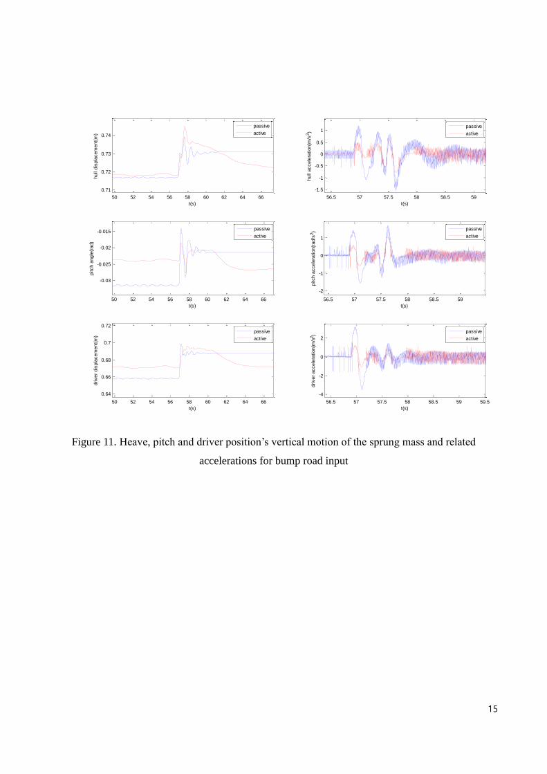
Time t is set to 0 when the vehicle starts to drive on the bump road. Simulation results of the heave,
pitch motions, the driver’s vertical position and corresponding accelerations for the bump road input
are given in Figure 11. It is seen from this figure that the magnitudes for the acceleration in the
driver’s position is significantly decreased. Also, the displacements and accelerations for our
adaptive controlled active suspensions vanish faster than the passive suspensions. These results
evince the efficiency of the reference changing adaptive controller. Specifically, decreased vertical
accelerations, as in Figure 11, indicate that the ride comforts are improved at driver and crew
member’s position. The frequency weighted RMS values for the heave, pitch and driver position’s
accelerations of the vehicle body are presented in Figure 12. The decrease in the RMS values is
between 46.71 % and 59.05 % which shows increased ride comfort of the vehicle. Peak values for
the heave, pitch and driver position’s accelerations are also depicted in Figure 12. Moreover, the
peak values of accelerations are decreased with suggested control method, that is, the maximum
accelerations sensed by the crew members and driver are decreased between 40.35 % and 49.81 %.
There is difference in initial vertical displacement of the driver between passive case and active case
because frir _ set the initial reference value of the front wheels’ arm angle. For the passive case, it
seems like road elevation occurred after bump road input. But this is because this road input result
slight change in arm angles of the vehicle and, consequently, shifted equilibrium point of the vehicle
due to changed geometry, as seen in Figure 13. The reference trajectory from reference calculator
and corresponding variation in arm angle is presented in Figure 14. It is clear that these reference
values give the controller the tendency of the control, although it is actually demanding controller to
exactly follow its given reference, which is almost impossible due to insufficient time to follow.
15
50 52 54 56 58 60 62 64 66
0.71
0.72
0.73
0.74
t(s)
hull
dis
pla
cem
ent(
m)
56.5 57 57.5 58 58.5 59
-1.5
-1
-0.5
0
0.5
1
t(s)
hull
accele
ration(m
/s2)
50 52 54 56 58 60 62 64 66
-0.03
-0.025
-0.02
-0.015
t(s)
pitch a
ngle
(rad)
56.5 57 57.5 58 58.5 59
-2
-1
0
1
t(s)
pitch a
ccele
ration(r
ad/s
2)
50 52 54 56 58 60 62 64 66
0.64
0.66
0.68
0.7
0.72
t(s)
driver
dis
pla
cem
ent(
m)
56.5 57 57.5 58 58.5 59 59.5
-4
-2
0
2
t(s)
driver
accele
ration(m
/s2)
passive
active
passive
active
passive
active
passive
active
passive
active
passive
active
Figure 11. Heave, pitch and driver position’s vertical motion of the sprung mass and related
accelerations for bump road input

16
passive active0
0.2
0.4
0.6
0.8
1
rms o
f hull
accele
ration(m
/s2)
X = 1
Y = 0.275
X = 2
Y = 0.133
passive active0
0.2
0.4
0.6
0.8
1
rms o
f pitch a
ccele
ration(r
ad/s
2)
X = 1
Y = 0.316
X = 2
Y = 0.169
passive active0
0.2
0.4
0.6
0.8
1
rms o
f driver
accele
ration(m
/s2)
X = 1
Y = 0.558
X = 2
Y = 0.229
passive active0
2
4
6
8
10
X = 1
Y = 1.57
peak o
f hull
accele
ration(m
/s2)
X = 2
Y = 0.788
passive active0
2
4
6
8
10
X = 1
Y = 1.71
peak o
f pitch a
ccle
ration(r
ad/s
2)
X = 2
Y = 1.02
passive active0
2
4
6
8
10
X = 1
Y = 3.5
peak o
f driver
accele
ration(m
/s2)
X = 2
Y = 1.88
Figure 12. RMS and peak values for the heave, pitch and driver accelerations for bump road input
40 45 50 55 60 65 70 75 80
0.25
0.3
0.35
t(s)
fr
ont(r
ad)
40 45 50 55 60 65 70 75 80
0.25
0.3
0.35
t(s)
m
id(r
ad)
Figure 13. Suspension arm angle of the vehicle on bump road input

17
56 56.5 57 57.5 58 58.5 59 59.5 60 60.5
-1.5
-1
-0.5
0
0.5
t(s)
r front
(rad)
front
(rad)
56 56.5 57 57.5 58 58.5 59 59.5 60 60.5-0.6
-0.4
-0.2
0
0.2
0.4
0.6
0.8
t(s)
r mid
(rad)
mid
(rad)
Figure 14. Reference trajectory and corresponding actual arm angle on bump road input
Next, the vehicle was simulated on a road input with limited ramp, Figure 15. This type of road
inputs usually used to test the performance of the suspension when the vehicle faces a sudden change
in the road surface elevation [27]. This type of road input also tests whether the suspension under
suggested controller preserves its working space since the inherent suspension working space of the
vehicle would not be changed while pushing up or pulling down the vehicle body in order to
compensate for the change in road elevation. The road input with limited ramp is formulated as
below where h is the final road surface elevation.
th
tth
t
y t
1.1,
1.11),1(10
10,0
)(0 (12)

18
219.8 220 220.2 220.4 220.6 220.8-0.65
-0.645
-0.64
-0.635
-0.63
-0.625
-0.62
-0.615
-0.61
distance(m)
road h
eig
ht(
m)
Figure 15. Road input with limited ramp
54 56 58 60 62 64 66 68 70 72 74
0.7
0.72
0.74
0.76
0.78
t(s)
hull
dis
pla
cem
ent(
m)
56.5 57 57.5 58 58.5 59
-1
-0.5
0
0.5
1
t(s)
hull
accele
ration(m
/s2)
48 50 52 54 56 58 60 62 64 66 68
-0.03
-0.025
-0.02
-0.015
-0.01
-0.005
t(s)
pitch a
ngle
(rad)
56.5 57 57.5 58 58.5 59-1.5
-1
-0.5
0
0.5
1
t(s)
pitch a
ccele
ration(r
ad/s
2)
50 55 60 65 70
0.66
0.68
0.7
0.72
t(s)
driver
dis
pla
cem
ent(
m)
56.5 57 57.5 58 58.5 59
-2
-1
0
1
2
3
t(s)
driver
accele
ration(m
/s2)
passive
active
passive
active
passive
active
passive
active
passive
active
passive
active
Figure 16. Time histories for the vehicle body heave, pitch and driver’s vertical motion and
corresponding accelerations for the road input with limited ramp
Simulation result for the vehicle body heave, pitch, driver’s vertical motions and corresponding

19
accelerations for the road input with limited ramp are presented in Figure 16. This figure clearly
shows that the target vehicle reaches the final height value of the road input with improved ride
comfort. Suspension deflections in both front and mid arm of the vehicle for this road input are given
in Figure 17. It is observed from this figure the suspension space needed to operate is preserved.
50 52 54 56 58 60 62 64 66 68 70
-0.1
-0.05
0
t(s)
front(r
ad)
50 52 54 56 58 60 62 64 66 68 70
-0.05
0
0.05
t(s)
mid
(rad)
Figure 17. Variation of the suspension deflections for the road input with limited ramp
Figure 18 presents the weighted RMS values for the heave, pitch and driver’s position
accelerations of the sprung mass for the road input with limited ramp. The ride comfort is improved
since the RMS values for the heave, pitch and driver accelerations of the sprung mass are decreased
between 39.41 % and 65.09 %. The peak values for the heave, pitch and driver accelerations of the
sprung mass are also shown in Figure 18. The reference trajectory from reference calculator and
corresponding variation in arm angle is presented in Figure 19.

20
passive active0
0.2
0.4
0.6
0.8
1
X = 1
Y = 0.153
rms o
f hull
accele
ration(m
/s2)
X = 2
Y = 0.0925
passive active0
0.2
0.4
0.6
0.8
1
rms o
f pitch a
ccele
ration(r
ad/s
2)
X = 1
Y = 0.202X = 2
Y = 0.0967
passive active0
0.2
0.4
0.6
0.8
1
rms o
f driver
accele
ration(m
/s2)
X = 1
Y = 0.393
X = 2
Y = 0.137
passive active0
2
4
6
8
10
X = 1
Y = 1.14
peak o
f hull
accele
ration(m
/s2)
X = 2
Y = 0.582
passive active0
2
4
6
8
10
X = 1
Y = 1.45
peak o
f pitch a
ccle
ration(r
ad/s
2)
X = 2
Y = 0.627
passive active0
2
4
6
8
10
X = 1
Y = 2.92
peak o
f driver
accele
ration(m
/s2)
X = 2
Y = 1.44
Figure 18. The RMS and peak values for the heave, pitch and driver accelerations for the road input
with limited ramp

21
56 56.5 57 57.5 58 58.5 59 59.5 60 60.5 61
-1.5
-1
-0.5
0
0.5
t(s)
r front
(rad)
front
(rad)
56 56.5 57 57.5 58 58.5 59 59.5 60 60.5 61
-0.6
-0.4
-0.2
0
0.2
0.4
0.6
t(s)
r mid
(rad)
mid
(rad)
Figure 19. Reference trajectory and corresponding actual arm angle on road type with limited ramp
Finally, for the time domain analysis, a sinusoidal road input is applied to the full vehicle model in
order to test the performance of the controller for severe periodic road conditions and to see the
capability of the controller keep a stable and comfortable reference value. The sinusoidal road input
to the front wheels is formulated as below with h being the magnitude of the road input:
)04.0())2
sin(1(2
)(0 hth
ty
(13)

22
215 220 225 230 235 240 245 250 255 260
-0.645
-0.64
-0.635
-0.63
-0.625
-0.62
-0.615
-0.61
distance(m)
road h
eig
ht(
m)
Figure 20. Sinusoidal road input
54 56 58 60 62 64 66 68 70
0.7
0.72
0.74
0.76
0.78
t(s)
hull
dis
pla
cem
ent(
m)
55 60 65 70
-0.5
0
0.5
1
t(s)
hull
accele
ration(m
/s2)
54 56 58 60 62 64 66 68 70
-0.04
-0.03
-0.02
-0.01
0
t(s)
pitch a
ngle
(rad)
55 60 65 70
-1
-0.5
0
0.5
t(s)
pitch a
ccele
ration(r
ad/s
2)
54 56 58 60 62 64 66 68 70
0.64
0.66
0.68
0.7
0.72
0.74
0.76
t(s)
driver
dis
pla
cem
ent(
m)
55 60 65 70-3
-2
-1
0
1
2
t(s)
driver
accele
ration(m
/s2)
passive
active
passive
active
passive
active
passive
active
passive
active
passive
active
Figure 21. Time histories for the vehicle body heave, pitch and driver’s vertical motion and
corresponding accelerations for the sinusoidal road input (velocity = 25km/h)

23
passive active0
0.2
0.4
0.6
0.8
1rm
s o
f hull
accele
ration(m
/s2)
X = 1
Y = 0.141 X = 2
Y = 0.0934
passive active0
0.2
0.4
0.6
0.8
1
rms o
f pitch a
ccele
ration(r
ad/s
2)
X = 1
Y = 0.0728X = 2
Y = 0.0522
passive active0
0.2
0.4
0.6
0.8
1
X = 1
Y = 0.187
rms o
f driver
accele
ration(m
/s2)
X = 2
Y = 0.0845
passive active0
2
4
6
8
10
X = 1
Y = 0.913
peak o
f hull
accele
ration(m
/s2)
X = 2
Y = 0.526
passive active0
2
4
6
8
10
X = 1
Y = 0.842
peak o
f pitch a
ccle
ration(r
ad/s
2)
X = 2
Y = 0.519
passive active0
2
4
6
8
10
peak o
f driver
accele
ration(m
/s2)
X = 1
Y = 2 X = 2
Y = 1.09
Figure 22. The RMS and peak values for the heave, pitch and driver accelerations for the sinusoidal
road input (velocity = 25km/h)

24
55 56 57 58 59 60 61 62 63 64 65
-0.6
-0.4
-0.2
0
0.2
0.4
0.6
0.8
t(s)
r front
(rad)
front
(rad)
55 56 57 58 59 60 61 62 63 64 65
-0.8
-0.6
-0.4
-0.2
0
0.2
0.4
0.6
0.8
t(s)
r mid
(rad)
mid
(rad)
Figure 23. Reference trajectory and corresponding actual arm angle on sinusoidal road input
(velocity = 25km/h)
25
45 45.5 46 46.5 47 47.5 48 48.5 49 49.5 50
0.7
0.72
0.74
0.76
0.78
0.8
t(s)
hull
dis
pla
cem
ent(
m)
45 46 47 48 49 50
-2
-1
0
1
2
3
t(s)
hull
accele
ration(m
/s2)
45 45.5 46 46.5 47 47.5 48 48.5 49 49.5 50
-0.03
-0.025
-0.02
-0.015
-0.01
-0.005
0
t(s)
pitch a
ngle
(rad)
45 46 47 48 49 50
-1.5
-1
-0.5
0
0.5
1
1.5
t(s)
pitch a
ccele
ration(r
ad/s
2)
45 45.5 46 46.5 47 47.5 48 48.5 49 49.5 50
0.66
0.68
0.7
0.72
0.74
0.76
t(s)
driver
dis
pla
cem
ent(
m)
45 45.5 46 46.5 47 47.5 48 48.5 49 49.5 50-3
-2
-1
0
1
2
t(s)
driver
accele
ration(m
/s2)
passive
active
passive
active
passive
active
passive
active
passive
active
passive
active
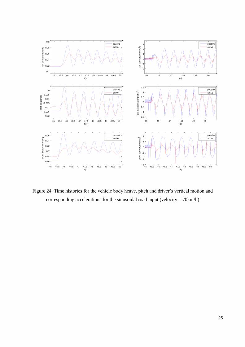
Figure 24. Time histories for the vehicle body heave, pitch and driver’s vertical motion and
corresponding accelerations for the sinusoidal road input (velocity = 70km/h)

26
passive active0
0.2
0.4
0.6
0.8
1
rms o
f hull
accele
ration(m
/s2)
X = 1
Y = 0.498
X = 2
Y = 0.164
passive active0
0.2
0.4
0.6
0.8
1
rms o
f pitch a
ccele
ration(r
ad/s
2)
X = 1
Y = 0.315
X = 2
Y = 0.162
passive active0
0.2
0.4
0.6
0.8
1
rms o
f driver
accele
ration(m
/s2)
X = 1
Y = 0.534
X = 2
Y = 0.139
passive active0
2
4
6
8
10
peak o
f hull
accele
ration(m
/s2)
X = 1
Y = 2.06X = 2
Y = 0.825
passive active0
2
4
6
8
10
peak o
f pitch a
ccle
ration(r
ad/s
2)
X = 1
Y = 1.31X = 2
Y = 0.91
passive active0
2
4
6
8
10
peak o
f driver
accele
ration(m
/s2)
X = 1
Y = 2.21 X = 2
Y = 1.38
Figure 25. The RMS and peak values for the heave, pitch and driver accelerations for the sinusoidal
road input (velocity = 70km/h)

27
45 45.5 46 46.5 47 47.5 48 48.5 49
-0.8
-0.6
-0.4
-0.2
0
0.2
0.4
0.6
0.8
1
t(s)
r front
(rad)
front
(rad)
45 45.5 46 46.5 47 47.5 48 48.5 49
-1
-0.5
0
0.5
1
t(s)
r mid
(rad)
mid
(rad)
Figure 26. Reference trajectory and corresponding actual arm angle on sinusoidal road input
(velocity = 70km/h)
Time responses for the driver and crew member’s vertical displacements and corresponding
accelerations for the sinusoidal road input are given in Figure 21. The improvement in the ride
quality with the active suspension increases substantially as the velocity of the vehicle increases, as
seen in Figure 24 and Figure 25. Substantial decreases in frequency weighted RMS values
demonstrate the usefulness of the suggested control method.
Figure 21 shows the weighted RMS values of the heave, pitch and driver acceleration of the
vehicle body. The frequency weighted RMS values have decreased between 28.36 % and 54.87 %
for the vehicle with speed of 25km/h, and 48.57% and 73.97% for the vehicle with speed of 70km/h.
Both results for different vehicle speeds prove the stability of the suggested algorithm. Figure 23
shows the reference trajectory and corresponding actual arm angles in the speed of 25km/h, while
Figure 26 shows it in the speed of 70km/h.

28
V. CONCLUSION
In this paper, first a non-linear quarter car vehicle model was derived and linearized around the
equilibrium point. Then it used adaptive law to estimate the plant parameter continuously, since there
exist some correlation between each wheel that should have taken into account. In particular, we
omitted using heave displacement as the measurable state, since not only it is costly, but also its
inaccuracy. According to the simulation results, the ameliorated adaptive linear quadratic control
methods gave better ride quality performance. Improvement in ride quality at passenger’s position is
pale in comparison with that in driver’s position since the behavior of last wheel, which is not
controlled with additional actuator but affects greatly in passenger’s ride quality, is not improved.
Extensive responses with different road conditions have indicated that the suggested ALQ controller,
without using heave sensor, is likely to provide fairly higher shooting accuracy/operational efficiency
and an increased rate of survivability in combat situations.
REFERENCES
[1] Howard, Geoffrey, John Peter Whitehead, and Donald Bastow. "Car Suspension and
Handling." Warrendale, PA: Society of Automotive Engineers, 2004. 474(2004).
[2] Rakheja, S., M. F. R. Afonso, and S. Sankar. "Dynamic analysis of tracked vehicles with trailing
arm suspension and assessment of ride vibrations."International Journal of Vehicle Design 13.1
(1992).
[3] Rae, W. J., and E. M. Kasprzak. "Kinematics of a double A-arm suspension, using Euler
orientation variables." SAE 2002 World Congress Detroit, Michigan. 2002.
[4] Peicheng, Shi, et al. "Kinematic analysis of a McPherson independent suspension." Journal of
Mechanical Transmission 1 (2008): 028.
[5] Deo, Hrishikesh V., and Nam P. Suh. "Axiomatic Design of Automobile Suspension and Steering
Systems: Proposal for a novel six-bar suspension."SAE SP (2004): 189-198.
[6] Jazar, Reza N. Vehicle dynamics: theory and application. Springer, 2008.
[7] Cronje, Paul Hendrik, and Pieter Schalk Els. "Improving off-road vehicle handling using an
active anti-roll bar." Journal of Terramechanics 47.3 (2010): 179-189.

29
[8] Rajamani, R. "Vehicle dynamics and control, 2006." 387-432.
[9] Hrovat, Davor. "Survey of advanced suspension developments and related optimal control
applications." Automatica 33.10 (1997): 1781-1817.
[10] Kim, Kiduck, and Doyoung Jeon. "Vibration suppression in an MR fluid damper suspension
system." Journal of intelligent material systems and structures10.10 (1999): 779-786.
[11] Petek, NiCholas K., et al. "Demonstration of an automotive semi-active suspension using
electrorheological fluid." SAE PUBLICATION SP 1074. NEW DEVELOPMENTS IN VEHICLE
DYNAMICS, SIMULATION, AND SUSPENSION SYSTEMS (SAE TECHNICAL PAPER
950586) (1995).
[12] Roh, H-S., and PARK YOUNGJIN. "Preview control of active vehicle suspensions based on a
state and input estimator." SAE transactions 107.6 (1998): 1713-1720.
[13] Araki, Yoshiaki, Masahiro Oya, and Hiroshi Harada. "Preview Control of Active Suspension
Using Disturbance of Front Wheel." International Symposium on Advanced Vehicle Control
(1994: Tsukuba-shi, Japan). Proceedings of the International Symposium on Advanced Vehicle
Control 1994. 1994
[14] LIAN, R. Enhanced Adaptive Self-Organizing Fuzzy Sliding-Mode Controller for Active
Suspension Systems. 2013.
[15] RYU, Seongpil; PARK, Youngjin; SUH, Moonsuk. Ride quality analysis of a tracked vehicle
suspension with a preview control. Journal of Terramechanics, 2011, 48.6: 409-417.
[16] WONG, J. Y. Dynamics of tracked vehicles. Vehicle system dynamics, 1997, 28.2-3: 197-219.
[17] Edara, Ramesh B. "Effective use of multibody dynamics simulation in vehicle suspension
system development." (2004).
[18] Ioannou, Petros A., and Jing Sun. Robust adaptive control. DoverPublications. com, 2012.
[19] RUSSELL, Stuart. Artificial intelligence: A modern approach, 2/E. Pearson Education India,
2003.
[20] CERONE, Vito. Linear quadratic control: An introduction. Prentice Hall, 1995.
[21] OLVER, Peter J.; SHAKIBAN, Chehrzad. Applied linear algebra. Prentice Hall, 2006.

30
[22] STRANG, Gilbert. Linear Algebra and Its Applications. Thomson–Brooks. Cole, Belmont, CA,
USA, 2005.
[23] SUN, Weichao, et al. Adaptive Backstepping Control for Active Suspension Systems With Hard
Constraints. 2013.
[24] International Organization for Standardization. Mechanical vibration and shock-Evaluation of
human exposure to whole-body vibration-Part 1: General requirements. The Organization, 1997.
[25] Paddan, G. S., and M. J. Griffin. "Evaluation of whole-body vibration in vehicles." Journal of
Sound and Vibration 253.1 (2002): 195-213.
[26] YAGIZ, Nurkan; HACIOGLU, Yuksel. Backstepping control of a vehicle with active
suspensions. Control Engineering Practice, 2008, 16.12: 1457-1467
[27] Yagiz, Nurkan, Ismail Yuksek, and Selim Sivrioglu. "Robust control of active suspensions for a
full vehicle model using sliding mode control." JSME international journal. Series C,
Mechanical systems, machine elements and manufacturing 43.2 (2000): 253-258..
[28] ZHANG, Xinjie, et al. Semi-Active Suspension Adaptive Control Strategy Based on Hybrid
Control. In: Proceedings of the FISITA 2012 World Automotive Congress. Springer Berlin
Heidelberg, 2013. p. 625-632.
[29] LIN, Jung-Shan; HUANG, Chiou-Jye. Nonlinear backstepping active suspension design applied
to a half-car model. Vehicle system dynamics, 2004, 42.6: 373-393.