ADAPTIVE CONFIDENCE INTERVALS FOR … Confidence... · Hansen and Stark (2005) that the ... example in the case that a conﬁdence interval has guaranteed coverage prob- ... The solution

Submitted to the Annals of Statistics

ADAPTIVE CONFIDENCE INTERVALS FOR

REGRESSION FUNCTIONS UNDER SHAPE

CONSTRAINTS

By T. Tony Cai, ∗ Mark G. Low and Yin Xia ∗

University of Pennsylvania

Adaptive confidence intervals for regression functions are con-structed under shape constraints of monotonicity and convexity. Anatural benchmark is established for the minimum expected length ofconfidence intervals at a given function in terms of an analytic quan-tity, the local modulus of continuity. This bound depends not only onthe function but also the assumed function class. These benchmarksshow that the constructed confidence intervals have near minimumexpected length for each individual function, while maintaining agiven coverage probability for functions within the class. Such adap-tivity is much stronger than adaptive minimaxity over a collection oflarge parameter spaces.

1. Introduction. The construction of useful confidence sets is one ofthe more challenging problems in nonparametric function estimation. Thereare two main interrelated issues which need to be considered together, cov-erage probability and the expected size of the confidence set. For a fixedparameter space it is often possible to construct confidence sets which haveguaranteed coverage probability over the parameter space while controllingthe maximum expected size. However such minimax statements are oftenthought to be too conservative and a more natural goal is to have the ex-pected size of the confidence set reflect in some sense the difficulty of esti-mating the particular underlying function.

These issues are well illustrated by considering confidence intervals forthe value of a function at a fixed point. Let Y be an observation from thewhite noise model:

(1) dY (t) = f(t)dt+ n− 12 dW (t), −1

2≤ t ≤ 1

2

∗The research of Tony Cai and Yin Xia was supported in part by NSF FRG GrantDMS-0854973.

AMS 2000 subject classifications: Primary 62G99; secondary 62F12,62F35,62M99Keywords and phrases: Adaptation, confidence interval, convex function, coverage

probability, expected length, minimax estimation, modulus of continuity, monotone func-tion, nonparametric regression, shape constraint, white noise model.

1imsart-aos ver. 2011/05/20 file: ConfidenceShapeAnnalsSubmission.tex date: May 17, 2012

2 T. TONY CAI, MARK G. LOW AND YIN XIA

where W (t) is standard Brownian motion and f belongs to some parameterspace F . Suppose that we wish to construct a confidence interval for f atsome point t0 ∈ (−1

2 ,12). Let CI be a confidence interval for f(t0) based on

observing the process Y and let L(CI) denote the length of the confidenceinterval. The minimax point of view can then be expressed by: subject tothe constraint on the coverage probability inff∈F P (f(t0) ∈ CI) ≥ 1 − α,minimize the maximum expected length supf∈F Ef (L(CI)).

As an example it is common to consider the Lipschitz classes

Λ(β,M) ={

f : |f(y)− f(x)| ≤ M |y − x|β for x, y ∈ [−12 ,

12 ]}

, if 0 < β ≤ 1

and for β > 1

Λ(β,M) ={

f : |f (⌊β⌋)(x)− f (⌊β⌋)(y)| ≤ M |x− y|β′

for x, y ∈ [−12 ,

12 ]}

,

where ⌊β⌋ is the largest integer less than β and β′ = β−⌊β⌋. For these classesit easily follows from results of Donoho (1994), Low (1997), and Evans,Hansen and Stark (2005) that the minimax expected length of confidenceintervals, which have guaranteed coverage of 1−α over Λ(β,M), is of order

M1

1+2β n− β

1+2β .It should however be stressed that confidence intervals which achieve such

an expected length rely on the knowledge of the particular smoothness pa-rameters β andM , which are not known in most applications. Unfortunately,Low (1997) and Cai and Low (2004) have shown that the natural goal ofconstructing an adaptive confidence interval which has a given coverageprobability and has expected length that is simultaneously close to theseminimax expected lengths for a range of smoothness parameters is not ingeneral attainable. More specifically suppose that a confidence interval hasguaranteed coverage probability of 1 − α over Λ(β,M). Then for any f inthe interior of Λ(β,M) the expected length for this f must also be of or-

der n− β

1+2β . In other words the minimax rate describes the actual rate forall functions in the class other than those on the boundary of the set. Forexample in the case that a confidence interval has guaranteed coverage prob-ability of 1− α over the Lipschitz class Λ(1,M) then even if the underlyingfunction has two derivatives and first derivative smaller than M , the confi-dence interval for f(x) must still have expected length of order n−1/3 eventhough one would hope that an adaptive confidence interval would have amuch shorter length of order n−2/5.

Despite these very negative results there are some settings where somedegree of adaptation has been shown to be possible. In particular under cer-tain shape constraints Hengartner and Stark (1995) and Dumbgen (1998)

imsart-aos ver. 2011/05/20 file: ConfidenceShapeAnnalsSubmission.tex date: May 17, 2012

ADAPTIVE CONFIDENCE INTERVALS 3

have shown that such extremely negative results do not hold. For exam-ple Hengartner and Stark (1995) constructed confidence bands which havea guaranteed coverage probability of at least 1 − α over the collection ofall monotone densities and which have maximum expected length of order

( log nn )β

2β+1 for those monotone densities which are in Λ(β,M) simultane-ously for 0 < β ≤ 1. These results are still framed in terms of the maximumlength over particular large parameter spaces but the existence of such in-tervals raises the question of exactly how much adaption is possible. It isthis question that is the focus of the present paper.

Rather than considering the maximum expected length over large collec-tions of functions we study the problem of adaptation to each and everyfunction in the parameter space. This problem is examined in detail for twocommonly used collections of functions that have shape constraints, namelythe collection of convex functions and the collection of monotone functions.We focus on these parameter spaces as it is for such shape constrained prob-lems for which there is some hope for adaptation. Within this context weconsider the problem of constructing a confidence interval for the value of afunction at a fixed point under both the white noise with drift model givenin (1) as well as a nonparametric regression model. We show that within theclass of convex functions and the class of monotone functions it is indeedpossible to adapt to each individual function, and not just to the minimaxexpected length over different parameter spaces in a collection.

This result is achieved in two steps. First we study the problem of mini-mizing the expected length of a confidence interval assuming that the datais generated from a particular function f in the parameter space, subject tothe constraint that the confidence interval has guaranteed coverage proba-bility over the entire parameter space. The solution to this problem gives abenchmark for the expected length which depends on the function f con-sidered. It gives a bound on the expected length of any adaptive intervalbecause if the expected length is smaller than this bound for any particularfunction, the confidence interval cannot have the desired coverage probabil-ity. In applications it is more useful to express the benchmark in terms of alocal modulus of continuity, an analytic quantity that can be easily calcu-lated for individual functions. In situations where adaptation is not possiblethis local modulus of continuity does not vary significantly from function tofunction. Such is the case in the settings considered in Low (1997). Howeverin the context of convex or monotone functions the resulting benchmarkdoes vary significantly and this opens up the possibility for adaptation inthose settings.

Our second step is to actually construct adaptive confidence intervals.



This is done separately for monotone functions and convex functions, withsimilar results. For example, an adaptive confidence interval is constructedwhich is shown to have expected length uniformly within an absolute con-stant factor of the benchmark for every convex function, while maintainingcoverage probability over the collection of all convex functions. In otherwords, this confidence interval has smallest expected length, up to a univer-sal constant factor, for each and every convex function within the class ofall confidence intervals which guarantee a 1 − α coverage probability overall convex functions. A similar result is established for a confidence intervaldesigned for monotone functions.

The rest of the paper is organized as follows. In section 2 the benchmarkfor the expected length at each monotone function or each convex func-tion is established under the constraint that the interval has a given levelof coverage probability over the collection of monotone functions or thecollection of convex functions. Section 3 constructs data driven confidenceintervals for both monotone functions and convex functions and shows thatthese confidence intervals maintain coverage probability and have expectedlength within an absolute constant factor of the benchmark given in Section2 for each monotone function and convex function. Section 4 considers thenonparametric regression model and Section 5 discusses connections of ourresults with other work in the literature. Proofs are given in Section 6.

2. Benchmark and Lower Bound on Expected Length. As men-tioned in the introduction, the focus in this paper is the construction ofconfidence intervals which have expected length that adapts to the unknownfunction. The evaluation of these procedures depends on lower bounds whichare given here in terms of a local modulus of continuity first introduced byCai and Low (2011) in the context of point estimation of convex functionsunder mean squared error loss. These lower bounds provide a natural bench-mark for our problems.

2.1. Benchmark and Lower Bound. We focus in this paper on estimatingthe function f at 0 since estimation at other points away from the boundaryis similar. For a given function class F , write Iα(F) for the collection of allconfidence intervals which cover f(0) with guaranteed coverage probabilityof 1 − α for all functions in F . For a given confidence interval CI, denoteby L(CI) the length of CI and L(CI, f) = Ef (L(CI)) the expected lengthof CI at a given function f . The minimum expected length at f of allconfidence intervals with guaranteed coverage probability of 1−α over F is



then given by

(2) L∗α(f,F) = inf

CI∈Iα(F)L(CI, f).

A natural goal is to construct a confidence interval with expected length closeto the minimum L∗

α(f,F) for every f ∈ F while maintaining the coverageprobability over F . However although L∗

α(f,F) is a natural benchmark forthe expected length of confidence intervals it is not easy to evaluate exactly.Instead as a first step towards our goal, we provide a lower bound for thebenchmark L∗

α(f,F) in terms of a local modulus of continuity ω(ǫ, f,F)introduced by Cai and Low (2011). The local modulus is a quantity that ismore easily computable and techniques for its analysis are similar to thosegiven in Donoho and Liu (1991) and Donoho (1994) where a global modulusof continuity was introduced in the study of minimax theory for estimatinglinear functionals. See the examples in Section 2.2.

For a parameter space F and function f ∈ F , the local modulus of con-tinuity is defined by

(3) ω(ǫ, f,F) = sup{|g(0) − f(0)| : ‖g − f‖2 ≤ ǫ, g ∈ F}.

where ‖ · ‖2 is the L2(−12 ,

12 ) function norm. The following theorem gives a

lower bound for the minimum expected length L∗α(f,F) in terms of the local

modulus of continuity ω(ǫ, f,F). In this theorem and throughout the paperwe write Φ for the cumulative distribution function and φ for the densityfunction of a standard normal density and set zα = Φ−1(1− α).

Theorem 1 Suppose F is a nonempty convex set. Let 0 < α < 12 and

f ∈ F . Then for confidence intervals based on (1),

(4) L∗α(f,F) ≥ (1− 1√

2πzα+

φ(zα)

zα− α)ω(

zα√n, f,F).

In particular,

(5) L∗α(f,F) ≥ (1 − 1√

2πzα)ω(

zα√n, f,F).

The lower bounds given in Theorem 1 can be viewed as benchmarks forthe evaluation of the expected length of confidence intervals when the truefunction is f for confidence intervals which have guaranteed coverage prob-ability over all of F . The bound depends on the underlying true function fas well as the parameter space F .

The bounds from Theorem 1 are general. In some settings they can beused to rule out the possibility of adaptation, whereas in other settings they



provide bounds on how much adaptation is possible. In particular the resultruling out adaptation over Lipschitz classes mentioned in the introductioneasily follows from this theorem. For example, consider the Lipschitz classΛ(β,M) and suppose that f is in the interior of Λ(β,M). Straightforwardcalculations similar to those given in Section 2.2 show that

(6) ω(ǫ, f,Λ(β,M)) ∼ Cǫ2β

2β+1 .

Now consider two Lipschitz classes Λ(β1,M1) and Λ(β2,M2) with β1 > β2.A fully adaptive confidence interval in this setting would have guaranteedcoverage of 1−α over Λ(β1,M1)∪Λ(β2,M2) and maximum expected length

over Λ(βi,Mi) of order nβi

2βi+1 for i = 1 and 2. However, it follows fromTheorem 1 and (6) that for all confidence intervals with coverage probabilityof 1− α over Λ(β2,M2), for every f ∈ Λ(β2,M

′) with M ′ < M2,

L∗α(f,Λ(β2,M2)) ≥ C(α)n

− β22β2+1

for some constant C(α) not depending on f . In particular this holds for allf ∈ Λ(β1,M1) ∩ Λ(β2,M

′) and hence

supf∈Λ(β1,M1)

infCI∈Iα(Λ(β1,M1)∪Λ(β2,M2))

L(CI, f) ≥ C(α)n− β2

2β2+1 ≫ n− β1

2β1+1 .

Therefore it is not possible to have confidence intervals with adaptive ex-pected length over two Lipschitz classes with different smoothness parame-ters.

In the present paper Theorem 1 will be used to provide benchmarks in thesetting of shape constraints. Denote by Fm and Fc respectively the collectionof all monotonically nondecreasing functions and the collection of all convexfunctions on [−1

2 ,12 ]. We shall now show that in these cases the modulus

and the associated lower bounds vary significantly from function to function.

2.2. Examples of Bounds For Monotone Functions and Convex Functions.We now turn to the application of the lower bound given in Theorem 1 in thecase of monotone functions and convex functions. Here we shall evaluate thelower bound for three particular families of functions yielding different ratesat which the expected length decreases to zero as the noise level decreases incontrast to the situation just described where the parameter space did nothave an order constraint. Two of the functions will be both monotonicallynondecreasing and convex. In this case the lower bound can also be quitedifferent depending on whether we assume the knowledge that f is convexor monotonically nondecreasing.



The key quantity that is needed in any application of Theorem 1 is thelocal modulus.We follow the same approach as given in Donoho (1994) wherea global modulus of continuity is considered for minimax estimation. In eachcase, for a given function f , we first minimize the L2 norm between a functiong ∈ F and the function f subject to the constraint that |g(0)−f(0)| = a forsome given value a > 0. From here it is easy to invert and thus maximize|g(0) − f(0)| given a constraint on the L2 norm between f and g.

Example 1 As a first example consider the linear function fk(t) = kt wherek ≥ 0 is a constant. This function is both monotonically nondecreasing andconvex.

First consider the collection of monotonically nondecreasing functions Fm.We shall treat separately the case k > 0 and the case k = 0. For themoment we shall take k > 0. Suppose that 0 < a ≤ k

2 . In this case fk ∈ Fm

and the function g that minimizes ‖g − fk‖2 subject to the constraint that|g(0) − fk(0)| = a is given by g(t) = fk(t) if t < 0, g(t) = a if 0 ≤ t ≤ b,and g(t) = fk(t) if t > b, where b satisfies fk(b) = a. The assumption that

a ≤ k2 guarantees b ≤ 1

2 . We then have ‖g−fk‖2 = a32/(3k)

12 . It follows that

if ǫ2 ≤ 124k

2

ω(ǫ, fk, Fm) = (3k)13 ǫ

23

and consequently for n ≥ 24z2αk2

, if k > 0

L∗α(fk, Fm) ≥ (1− 1√

2πzα)(3k)

13 z

23αn

− 13 .

In the case that k = 0 a function g that minimizes ‖g−f0‖2 subject to theconstraint that |g(0) − f0(0)| = a is given by g(t) = f0(t) if t < 0, g(t) = aif 0 ≤ t ≤ 1

2 . In this case it is easy to check that ‖g − f0‖2 = 1√2ǫ and hence

ω(ǫ, f0, Fm) =√2ǫ

and hence

L∗α(f0, Fm) ≥ (1− 1√

2πzα)√2zαn

− 12 .

We now consider the bound for the length of the confidence interval for fkbelonging to the collection of convex functions. In this case we do not needto treat the cases k > 0 and k = 0 separately. The function g that minimize‖g − fk‖2 subject to the constraint that g is convex and |g(0) − fk(0)| = ais given by g(t) = (k + 3a)t− a if t ≥ 0 and g(t) = (k − 3a)t− a if t < 0. Inthis case ‖g − f‖2 = 1

2a. It then immediately follows that

ω(ǫ, fk, Fc) = 2ǫ



and so

L∗α(fk, Fc) ≥ (1− 1√

2πzα)2zαn

− 12 .

It is important to note that for k > 0 the minimum expected lengthsL∗α(fk, Fm) and L∗

α(fk, Fc) are different, one of order n− 13 and another of

order n− 12 , although the function fk is the same. It is also interesting to

note that the expected length of the confidence for monotone functions isan increasing function of k whereas the expected length of the confidencefor convex functions does not depend on k. Since we shall show that thesebounds are achievable within a constant factor it follows that the mini-mum expected length of the confidence interval when fk is the true functiondepends strongly on whether we specify that the underlying collection offunctions is convex or monotone.

Example 2 As a second example which is also both monotonically nonde-creasing and convex consider the function f(t) = k1t + k2t

rI(0 < t ≤ 12)

where r ≥ 1 and k1 ≥ 0 and k2 > 0 are constants.We consider the cases r = 1 and r > 1 separately. When r = 1 the

function is piecewise linear with the change of slope at 0. In this case suppose0 < a ≤ k1+k2

2 . The monotonically nondecreasing function g ∈ Fm thatminimize ‖g − f‖2 subject to the constraint that |g(0) − f(0)| = a is givenby g(t) = f(t) if t < 0, g(t) = a if 0 ≤ t ≤ b, and g(t) = f(t) if t > b, whereb satisfies f(b) = a. The constraint a ≤ k1+k2

2 is to guarantee that such a b

exists with b ≤ 12 . Then we have ‖g− f‖2 = a

32 (3(k1 + k2))

− 12 and it follows

that if ǫ2 ≤ 124 (k1 + k2)

2

ω(ǫ, f, Fm) = (3(k1 + k2))13 ǫ

23

and consequently for n ≥ 24z2α(k1+k2)2

,

L∗α(f, Fm) ≥ (1− 1√

2πzα)(3(k1 + k2))

13 z

23αn

− 13 .

We can also give a lower bound on the expected length for this samefunction for confidence intervals which guarantee coverage over the class ofconvex functions. Suppose 0 < a ≤ k2

4 . Here we need to find the convex hthat minimizes ‖h − f‖2 subject to the constraints that |h(0) − f(0)| = a.It is given by h(t) = f(t) if t ≤ −2a

k2, h(t) = (k22 + k1)t+ a if −2a

k2≤ t ≤ 2a

k2

and h(t) = f(t) if t ≥ 2ak2. Then ‖f − g‖2 = 2a

32 /(3k2)

12 and it follows that

if ǫ2 ≤ k2248 ,

ω(ǫ, f, Fc) = (3k2/4)13 ǫ

23 .



Hence, for n ≥ 48z2αk22

,

L∗α(f, Fc) ≥ (1− 1√

2πzα)(3k2/4)

13 z

23αn

− 13 .

We now turn to the case where r > 1. Suppose 0 < a ≤ k12 +k2(

12)

r. In thiscase the monotonically nondecreasing function g that minimizes ‖g − f‖2subject to the constraints that |g(0) − f(0)| = a is given by g(t) = f(t) ift < 0, g(t) = a if 0 ≤ t ≤ b, and g(t) = f(t) if t > b, where b satisfiesf(b) = a. As before the condition 0 < a ≤ k1

2 + k2(12 )

r guarantees that b

exists with b < 12 . In this case a

32 (3k1)

− 12 −cas ≤ ‖g−f‖2 ≤ a

32 (3k1)

− 12 +cas

for some constant c > 0 and s > 3/2. It follows that if ǫ2 ≤ 124k

21 + (1 +

12r+1 − 2

r+1)(12)

2r+1k22 + (12 − 1r+1 +

1r+2)(

12)

r+1k1k2, then

ω(ǫ, f, Fm) = (3k1)13 ǫ

23 (1 + o(1)).

Hence,

L∗α(f, Fm) ≥ (1− 1√

2πzα)(3k1)

13 z

23αn

− 13 (1 + o(1)).

For a bound on the expected length of this same function for confidenceintervals with coverage guaranteed over the collection of convex functionswe suppose 0 < a ≤ k2(

12 )

r+1. In this case the convex function h thatminimizes ‖h−f‖2 subject to the constraints that |h(0)−f(0)| = a, is givenby h(t) = kt + a, k > k1, if x0 ≤ t ≤ x1 and h(t) = f(t) otherwise, where(x0, cx0) and (x1, cx1 + xr1) are the intersection points of f(t) and the linekt+ a. Then the function h with slope k0 that minimize ‖h− f‖2 would be

the least favorable function. It follows that, if ǫ2 ≤ k2224 (

12 )

2r,

ω(ǫ, f, Fc) = C(r)k1

2r+1

2 ǫ2r

2r+1

and consequently for n ≥ 24z2α22r

k22,

L∗α(f,Fc) ≥ (1− 1√

2πzα)C(r)k

12r+1

2 z2r

2r+1α n− r

2r+1 ,

where C(r) > 0 is a constant depending on r only.

It is interesting to note that in this example the rates of convergence forL∗α(f,Fm) and L∗

α(f,Fc) are the same for the case r = 1, and are differentwhen r > 1.

As a final example we consider a function which is monotonically nonde-creasing but not convex.



Example 3 Let f(t) = ktr for some constant k > 0 and r = 2l + 1 orr = 1

2l+1 for l = 0, 1, 2, · · · . Suppose that a < (12 )rk. In this case the function

g that minimizes ||g− f ||2 subject to the constraint that |g(0)− f(0)| = a isgiven by g(t) = f(t) if t < 0, g(t) = a if 0 ≤ t ≤ b, and g(t) = f(t) if t > b,where b satisfies f(b) = a. As before the condition a < (12)

rk guarantees

that b exists with b < 12 . Then ||g − f ||2 = a1+

12r /k

12r (2r2/(r + 1)(2r + 1))

12

and it follows that when ǫ2 ≤ (12 )2r+1k2 2r2

(r+1)(2r+1) ,

ω(ǫ, f, Fm) = ((r + 1)(2r + 1)k

2r2)

r2r+1 ǫ

2r2r+1 .

Hence for n ≥ 22r+1(r+1)(2r+1)z2α2r2k2

,

L∗α(f,Fc) ≥ (1− 1√

2πzα)((r + 1)(2r + 1)k

2r2)

r2r+1 z

2r2r+1α n− r

2r+1

and once again it is clear that the rate at which the expected length decreasesto zero depends strongly on the value of r.

Finally we should mention that in these examples, the local modulus ofcontinuity are calculated explicitly. However in general, the modulus can bedifficult to compute exactly. In such cases although some precision is lostthere is a simple method to bound the modulus within a constant factor forboth monotone functions and convex functions and in particular it is stilleasy to characterize the optimal rate of convergence for particular functions.See Section 5 for more discussions.

3. Confidence Procedures. In this section we both construct andgive an analysis of adaptive confidence intervals for monotone functions andconvex functions. The procedures are easily implementable. We considerthe class of monotonically nondecreasing functions and the class of convexfunctions. Concave functions and monotonically nonincreasing functions canbe handled similarly.

3.1. Construction. The construction is split into two steps. In the firststep a countable collection of confidence intervals is created each of which hasguaranteed coverage probability. These intervals are based on a collectionof pairs of linear estimators. For each interval one of the estimators hasnonnegative bias and the other nonpositive bias. The one sided control ofthe bias of these estimators is a key special feature in these problems andan important part of what makes it possible to adapt to every individual



function. Moreover for each function f this collection has at least one intervalwith expected length within a constant factor of the local modulus boundgiven in Theorem 1. The second step is to select from this collection aparticular interval.

In the case of monotonically nondecreasing functions we take for each j ≥2, pairs of estimators δRj = 2j(Y (2−j)−Y (0)) and δLj = 2j(Y (0)−Y (−2−j)).

Then for estimating f(0) it is easy to check that δRj has nonnegative and

monotonically nonincreasing biases while δLj have nonpositive and mono-tonically nondecreasing biases. The one sided control of the biases of theseestimators over the class of all monotonically nondecreasing functions easilyallows for the construction of a confidence interval. For that we shall needthe standard deviation of δRj and δLj . In order to give a unified treatmentin both the monotone and convex case it is useful to establish a commonnotation. Here we shall set σ2

j = 2j−1

n . It is then easy to check that both δRjand δLj have a standard deviation of

√2σj. It is then also easy to see that

for each j ≥ 2, the confidence interval CImj (α) given by

(7) CImj (α) = [δLj − zα/2√2σj , δ

Rj + zα/2

√2σj ]

has guaranteed coverage of 1−α. We should however note that in (7) the leftendpoint of the interval may be larger than the right end point in which casewe adopt the convention that the confidence interval is just the empty set.The length of this confidence interval is then max(δRj − δLj + 2

√2zα/2σj , 0).

In the case of convex functions for j ≥ 1 let δj = 2j−1(Y (2−j)−Y (−2−j))and let δj = 2δj+1−δj . As before it is easy to check that for convex functionsδj have nonnegative and monotonically nonincreasing biases and that δj havenonpositive and monotonically nondecreasing bias. See, for example, Lemma2 in Cai and Low (2011). It is also easy to check that the standard deviation

of δj is equal to σj where σ2j = 2j−1

n and that 2δj+1 − δj has a standard

deviation of√5σj . It then follows from the signs of the biases of δj+1 and

2δj+1 − δj that for any given j

(8) CIcj (α) = [2δj+1 − δj − zα/2√5σj, δj+1 + zα/2σj+1]

gives a confidence interval with coverage probability of at least 1 − α. Weshould also note once again that the left endpoint of the interval may belarger than the right end point in which case the confidence interval is takento be the empty set and so in this case the length of this confidence intervalis max(δj − δj+1 + (

√5 +

√2)zα/2σj , 0).

These results, for which a more formal proof is given in Section 6 aresummarized in the following proposition.



Proposition 1 For every j ≥ 2, the confidence interval CImj defined in (7)has coverage probability of at least 1−α for all monotonically nondecreasingfunction f ∈ Fm and for every j ≥ 1, the confidence interval CIcj defined in(8) has coverage probability of at least 1−α for all convex functions f ∈ Fc.

The second stage in the construction is that of selecting from these col-lections of intervals the one to be used. First note that one should not selectthe shortest interval since the collections defined in (7) and (8) will alwayscontain one which corresponds to the empty set. A more sensible goal is totry to select the interval with the smallest expected length or at least onewhich has expected length close to the smallest expected length.

The approach we take here is to choose an interval for which the expectedlength is of the same order of magnitude as the standard deviation of thelength. Such an interval will always have expected length close to the shortestexpected length. For the case of monotonically nondecreasing functions theselection of the interval from the countable collection in (7) can be done bycreating another collection of estimators which can be used to estimate theexpected length of the intervals.

More specifically set ξj = 2j−1(Y (2−j+1) − Y (2−j)) − 2j−1(Y (−2−j) −Y (−2−j+1)). Then for j ≥ 2, ξj’s are independent of each other and bothδRj and δLj are independent of ξk for every k ≤ j. We should note that

the estimators ξj are similar to δRj − δLj in that they are both differencesof averages of Y to the left and right of the origin and thus estimate theaverage local change of the function. However δRj − δLj are not independentfor different j whereas the ξj are independent. It is thus natural to view theξj as a surrogate for δRj − δLj with the technical advantage that they areindependent. The selection of a j for which ξj has expected value close toσj will then result in a confidence interval CImj close to the one with thesmallest expected length. The independence properties of the ξj allows usto guarantee a 1− α coverage probability while making this selection.

More specifically the construction proceeds as follows. Let

(9) j = infj

{

j : ξj ≤3

2zασj

}

and define the final confidence interval by

(10) CIm∗ = CImj(α)

Before we turn to the analysis of this procedure we also introduce here arelated confidence procedure in the convex case. Here rather than introduc-ing an independent estimate of the difference between the two estimators



used in constructing the confidence interval we proceed more directly. Thebasic idea is similar but the dependence between the estimates of j and theconfidence interval constructed from this estimate requires that we adjustthe original coverage level of our CIcj .

More specifically let Tj = δj − δj+1. When the expected value of Tj is thesame order as σj , the confidence interval CIcj will then be close to the onewith the smallest expected length. Our estimate of j is given by an empiricalversion, namely

(11) j = infj{j : Tj ≤ zασj}

Although this estimate can be used to select the appropriate CIcj to use,as just mentioned, care also needs to be taken to make sure that the resultingselected interval maintains the required coverage probability. The analysisgiven below shows that a choice of α/6 in the construction of the originalcollection of intervals guarantees an overall coverage probability of α. Thusin the case of convex functions we define our interval by

(12) CIc∗ = CIcj(α

6)

3.2. Analysis of the Confidence Intervals. In this section we present theproperties of the confidence intervals CIm∗ and CIc∗ defined by (10) and (12)focusing on the coverage and the expected length of these intervals.

We begin with the confidence interval CIm∗ . In this case it is easy to checkthe coverage probability of CIm∗ by the independence of the interval CImjand ξk for every k satisfying 2 ≤ k ≤ j.

The key to the analysis of the expected length is the introduction of jm∗where

(13) jm∗ = argminj

{j : Eξj ≤ zασj} .

The analysis of the expected length relies on showing that j is highlyconcentrated around jm∗ . The concentration of j around jm∗ then providesa bound on the expected length of CI∗. These results, for which a proof isgiven in Section 6 are summarized in the following theorem.

Theorem 2 Let 0 < α ≤ 0.2. The confidence interval CIm∗ defined in (10)has coverage probability of at least 1−α for all monotonically nondecreasingfunctions f ∈ Fm and satisfies

EfL(CIm∗ ) ≤ 1.21(3zα + 2√2zα

2)σjm

∗≤ c0zασjm

∗,(14)

where c0 is a constant and can be taken to be 8.85 for all 0 < α ≤ 0.2.



Remark 1 The constant c0 in Theorem 2 depends on the upper limit ofα. c0 can be smaller if the upper limit on α is reduced. For example, forcommon choices of α = 0.05 or 0.01, c0 ≤ 7.71 for α = 0.05, and c0 ≤ 7.42for α = 0.01.

Theorem 2 shows that the coverage probability is attained and also pro-vides an upper bound on the expected length in terms of σjm

∗. In order to to

establish that this expected length is within a constant factor of the lowerbound given in Theorem 1, we need to provide a lower bound for L∗

α(f, Fm)in terms of zασjm

∗. This connection is given in the following theorem.

Theorem 3 Let 0 < α ≤ 0.2 and let f ∈ Fm. Then

(15) L∗α(f, Fm) ≥ (1− 1√

2πzα)1√2zασjm

∗.

Combining Theorems 2 and 3, we have

(16) EfL(CIm∗ ) ≤ c1L∗α(f, Fm)

for all monotonically nondecreasing function f ∈ Fm, where c1 is a constantdepending on α only. For example, c1 can be taken to be 14.40 for α = 0.05and 12.67 for α = 0.01. Hence, the confidence interval CIm∗ is uniformlywithin a constant factor of the benchmark L∗

α(f, Fm) for all monotonicallynondecreasing functions f and all confidence level 1− α ≥ 0.8.

We now turn to an analysis of the properties of the confidence intervalCIc∗ defined in (12). The key to this analysis is the introduction of jc∗ where

(17) jc∗ = argminj

{

j : ETj ≤2

3zασj

}

.

The analysis of both the coverage probability and the expected lengthrelies on showing that j is highly concentrated around jc∗. The probabilityof not covering f(0) can be bounded by

(18) P (f(0) /∈ CIc∗) ≤ P (j ≤ jc∗−3)+P (j ≥ jc∗+3)+2∑

l=−2

P (f(0) /∈ CIjc∗+l).

The first two terms are controlled by the high concentration of j around jc∗and the last term is controlled by Proposition 1 which bounds the coverageprobability of any given j. The concentration of j around jc∗ also allowscontrol on the expected length of CIc∗ which leads to the following theorem.



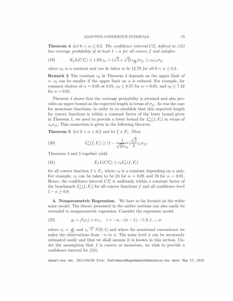
Theorem 4 Let 0 < α ≤ 0.2. The confidence interval CIc∗ defined in (12)has coverage probability of at least 1− α for all convex f and satisfies

(19) EfL(CIc∗) ≤ 1.25(zα + (√5 +

√2)z α

12)σjc

∗≤ c0zασjc

∗

where c0 is a constant and can be taken to be 12.79 for all 0 < α ≤ 0.2.

Remark 2 The constant c0 in Theorem 4 depends on the upper limit ofα. c0 can be smaller if the upper limit on α is reduced. For example, forcommon choices of α = 0.05 or 0.01, c0 ≤ 8.57 for α = 0.05, and c0 ≤ 7.42for α = 0.01.

Theorem 4 shows that the coverage probability is attained and also pro-vides an upper bound on the expected length in terms of σjc

∗. As was the case

for monotone functions, in order to to establish that this expected lengthfor convex functions is within a constant factor of the lower bound givenin Theorem 1, we need to provide a lower bound for L∗

α(f, Fc) in terms ofzασjc

∗. This connection is given in the following theorem.

Theorem 5 Let 0 < α ≤ 0.2 and let f ∈ Fc. Then

(20) L∗α(f, Fc) ≥ (1− 1√

2πzα)

√2

3zασjc

∗.

Theorems 4 and 5 together yield

(21) EfL(CIc∗) ≤ c2L∗α(f, Fc)

for all convex function f ∈ Fc, where c2 is a constant depending on α only.For example, c2 can be taken to be 24 for α = 0.05 and 19 for α = 0.01.Hence, the confidence interval CIc∗ is uniformly within a constant factor ofthe benchmark L∗

α(f, Fc) for all convex functions f and all confidence level1− α ≥ 0.8.

4. Nonparametric Regression. We have so far focused on the whitenoise model. The theory presented in the earlier sections can also easily beextended to nonparametric regression. Consider the regression model

(22) yi = f(xi) + σzi, i = −n,−(n− 1),−1, 0, 1, ..., n

where xi =i2n and zi

iid∼ N(0, 1) and where for notational convenience weindex the observations from −n to n. The noise level σ can be accuratelyestimated easily and thus we shall assume it is known in this section. Un-der the assumption that f is convex or monotone, we wish to provide aconfidence interval for f(0).



4.1. Monotone Regression. Let J = ⌊log2 n⌋. For 1 ≤ j ≤ J define thelocal average estimators

(23) δRj = 2−j+12j−1∑

k=1

yk and δLj = 2−j+12j−1∑

k=1

y−k.

We should note that the indexing scheme is the reverse of that given for thewhite noise with drift process. Here estimators δRj (or δLj ) with small valuesof j have smaller bias (or larger bias) and larger variance than those withlarger values of j.

As in the white noise model it is easy to check that δRj has nonnegative bias

and δLj has nonpositive bias. Simple calculations show that the variance of

δRj and δLj are both 2σ2j , where σ

2j = 2−jσ2. It is also important to introduce

ξj as in the white noise case, where ξj = 2−j∑2j

k=2j−1+1(yk− y−k). It is easyto check that Eξj ≤ Eξj+1, ξj’s are independent with each other and bothδRj and δLj are independent with ξk for every k ≥ j.

It then follows that CImj = [δLj − zα2

√2σj , δ

Rj + zα

2

√2σj ] has guaranteed

coverage probability of at least 1 − α over all monotonically nondecreasingfunctions.

Now set

(24) j = maxj

{

j : ξj ≤3

2zασj

}

and define the confidence interval to be

(25) CIm∗ = CImj.

The properties of this confidence interval can then be analyzed in the sameway as before and can be shown to be similar to those for the white noisemodel. In particular, the following result holds.

Theorem 6 Let 0 < α ≤ 0.2. The confidence interval CIm∗ defined in (25)has coverage probability of at least 1 − α for all monotone function f andsatisfies

(26) EfL(CIm∗ ) ≤ C1L∗α(f, Fm)

for all monotonically nondecreasing function f ∈ Fm, where C1 > 0 is aconstant depending on α only.



4.2. Convex Regression. As in the monotone case, set J = ⌊log2 n⌋. For1 ≤ j ≤ J define the local average estimators

(27) δj = 2−j2j−1∑

k=1

(y−k + yk).

We should note that this indexing scheme is the reverse of that given forthe white noise with drift process. Here estimators δj with small values of jhave smaller bias and larger variance than those with larger values of j.

As in the white noise model it is easy to check that δj has nonnegative bias.It is also important to introduce an estimate which has a similar variancebut is guaranteed to have nonpositive bias. The key step is to introduce

(28) Tj = δj − δj−1,

as an estimate of the bias of δj . The following lemma from Cai and Low(2011) gives the required properties of δj and Tj .

Lemma 1 For any convex function f ,

2ETj ≤ ETj+1(29)

Bias(δj) ≤ 2j−1 + 1

2j + 1Bias(δj+1)(30)

2j−2

2j−1 + 1Bias(δj) ≤ ETj ≤ Bias(δj).(31)

The estimators δj have nonnegative and monotonically nondecreasing biases.On the other hand, it follows from (30) that the estimator

δLj = (2 + 2−(j−1))δj − (1 + 2−(j−1))δj+1 = δj − (1 + 2−(j−1))Tj+1

has a nonpositive and monotonically nonincreasing bias. Simple calculationsshow that the variance of δLj is τ2j = (5 + 2−j+3 + 2−2j+2)2−j−1σ2.

It then follows that CIcj = [δj − (1 + 2−(j−1))Tj+1 − zα/12τj, δj + zα/12σj ]has coverage over all convex functions.

Now set

(32) j = maxj

{j : Tj ≤ zασj}

and define the confidence interval to be

(33) CIc∗ = CIcj.

This confidence interval shares similar properties as the one for the whitenoise model. In particular, the following result holds.



Theorem 7 Let 0 < α ≤ 0.2. The confidence interval CIc∗ defined in (33)has coverage probability of at least 1−α for all convex function f and satisfies

(34) EfL(CIc∗) ≤ C2L∗α(f, Fc)

for all convex function f ∈ Fc, where C2 > 0 is a constant depending on αonly.

5. Discussions. The major emphasis of the paper has been to showthat with shape constraints it is possible to construct confidence intervalsthat have expected length that adapts to individual functions. In this sectionwe shall discuss briefly how our results relate to the commonly consideredminimax point of view and we shall explain how our results can be extendedto the problem of estimating the value of f at points other than 0. Finallywe also discuss in this section how the lower bounds described in terms ofthe local modulus of continuity can be bounded conveniently by a functionwhich is easy to compute even when explicit calculation of the modulus isdifficult.

5.1. Minimax results. Although the focus of the present paper has beenon the construction of a confidence interval with the expected length adap-tive to each individual convex or monotone function, these results do yieldimmediately adaptive minimax results for the expected length in the con-ventional sense. Define

Fc(β,M) = Fc ∩ Λ(β,M) and Fm(β,M) = Fm ∩ Λ(β,M).

The following results are direct consequence of Theorems 2 and 4.

Corollary 1 (i). The confidence interval CIm∗ defined in (10) satisfies

(35) supf∈Fm(β,M)

EfL(CIm∗ ) ≤ C1M1

1+2β n− β

1+2β .

simultaneously for all 0 ≤ β ≤ 1 and 1 < M < ∞, for some absoluteconstant C1 > 0.

(ii). The confidence interval CIc∗ defined in (12) satisfies

(36) supf∈Fc(β,M)

EfL(CIc∗) ≤ C2M1

1+2β n− β

1+2β .

simultaneously for all 1 ≤ β ≤ 2 and 1 < M < ∞, for some absoluteconstant C2 > 0.



We should note that these ranges of Lipschitz classes are the only ones ofinterest in these cases. In particular suppose that CI is a confidence inter-val with guaranteed coverage over the class of monotonically nondecreasingfunctions. Then for any β > 1 the class Λ(β,M) includes the linear functionfk(t) = kt. As shown in Example 1 in Section 2.2

L∗α(fk, Fm) ≥ (1− 1√

2πzα)(3k)

13 z

23αn

− 13 .

Hence,(37)

supf∈Fm(β,M)

EfL(CI) ≥ supk

L∗α(fk, Fm) = sup

k(1− 1√

2πzα)(3k)

13 z

23αn

− 13 = ∞.

A similar results holds for convex functions assumed to belong to Λ(β,M)with β > 2. On the other hand suppose f is convex and assumed to belongto Λ(β,M) with β < 1. Then from the assumption that f is in Λ(β,M)it follows that |f(1/2) − f(−1/2)| ≤ M . Convexity then shows that f ∈Λ(1,M) and the maximum expected length over this class is given above.

5.2. Calculations of the local modulus of continuity. In section 2 we in-troduced a lower bound for the smallest expected length of a confidenceinterval. The lower bound is given in terms of a local modulus of continuity.We also illustrated how such a bound could be applied in the context ofmonotone and convex functions. In general exact evaluation of the modulusof continuity is difficult because it involves a search over all other functionsin the parameter space. However in the context of the collection of mono-tone functions or the collection of convex functions it is possible to boundthe modulus in an easy and useful way based only on evaluating the actualfunction.

We first consider convex functions. The local modulus of continuity forconvex functions was bounded in Cai and Low (2011) in terms of the fol-lowing K function

K(t) =t

√

H−1(t),

where fs(t) = f(t)+f(−t)2 − f(0), H(t) =

√tfs(t) for 0 ≤ t ≤ 1/2 and

H−1(x) = sup{t : 0 ≤ t ≤ 1/2,H(t) ≤ x}. The bounds for the localmodulus of continuity then can be summarized in the following propositionwhich has been proved in Cai and Low (2011).



Proposition 2 For ǫ > 0 and f ∈ Fc,

K(2√3ǫ) ≤ ω(ǫ, f, Fc) ≤ K(

√

10

3ǫ).

A similar approach can also be used to introduce a K function in thecontext of monotone nondecreasing functions. For each function f ∈ Fm,define

fs(t) =|f(t)− f(−t)|

2

for 0 ≤ t ≤ 12 . It is easy to see that fs is monotonically nondecreasing. For

every ǫ > 0, let

a∗(ǫ) = sup

{

a : (1

a

∫ 2a

afs(t)dt)

2 ≤ 1

aǫ2}

,

and defineK(ǫ) =

ǫ√

a∗(ǫ).

It is clear that K only depends on the function f . In the following proposi-tion, it is shown that the local modulus of continuity of monotone functionscan be bounded by this K function.

Proposition 3 For ǫ > 0 and f ∈ Fm,

(38) K(1√2ǫ) ≤ ω(ǫ, f, Fm) ≤ 4K(

1

2ǫ).

5.3. Confidence interval at other points. The focus of the present pa-per has been on the problem of estimating the value of f(0). The basicdevelopment is similar for any other point t in the interior of the inter-val [−1/2, 1/2] unless t is near to the boundary. More specifically for any0 ≤ t < 1/2 we can consider estimators δRj (t) = 2j(Y (t + 2−j) − Y (t)) and

δLj (t) = 2j(Y (t) − Y (t− 2−j)) where j ≥ − log2(14 − t

2) for monotone func-

tions and δj(t) = 2j−1(Y (t+2−j)− Y (t− 2−j)) where j ≥ − log2(12 − t) for

convex functions. The basic theory is the same as before.For monotonically nondecreasing functions, the confidence interval CImj

is replaced by

CImj (t) = [δLj (t)− zα2

√2σj , δ

Rj (t) + zα

2

√2σj]

and the choice of j is given by

j(t) = infj≥− log2(

14− t

2)

{

j : ξj(t) ≤3

2zασj

}

,



where ξj(t) = 2j−1(Y (t + 2−j+1) − Y (t + 2−j)) − 2j−1(Y (t − 2−j) − Y (t −2−j+1)). The final confidence interval is defined by

(39) CIm∗ = CImj(t)

.

For convex functions, the confidence interval CIcj is replaced by

CIcj (t) = [δj+1(t)− (δj(t)− δj+1(t))+ − z α12

√5σj , δj+1(t) + z α

12σj+1]

and j is chosen to be

j(t) = infj≥− log2(

12−t)

{j : Tj(t) ≤ zασj} .

Define the final confidence interval by

CIc∗ = CIcj(t)

.

The modulus of continuity defined in (40) is replaced by

(40) ω(ǫ, f, t,F) = sup{|g(t) − f(t)| : ‖g − f‖2 ≤ ǫ, g ∈ F}.

The earlier analysis then yields

EfL(CIm∗ (t)) ≤ c1L∗α(f, t, Fm),

andEfL(CIc∗(t)) ≤ c2L

∗α(f, t, Fc),

where we now have

L∗α(f, t,F) ≥ (1 − 1√

2πzα)ω(

zα√n, f, t,F).

Finally we should note that at the boundary the construction of a con-fidence interval must be unbounded. For example any honest confidenceinterval for f(1/2) must be of the form [f(1/2),∞), otherwise it cannothave guaranteed coverage probability.

6. Proofs. We prove the main results in this section. We shall omitthe proofs for Theorems 6 and 7 as they are analogous to those for thecorresponding results in the white noise model.



6.1. Proof of Theorem 1. Suppose that X ∼ N(θ, σ2) where it is knownthat θ ∈ [0, aσ]. The confidence interval for θ which has guaranteed coverageover the interval θ ∈ [0, aσ] and which minimizes the expected length whenθ = 0 is given by

(41) [0,max(0,min(X + zασ, aσ))]

It follows that

(42) L = σ

∫ a−zα

−zα

zφ(z)dz+σ(zαP (−zα ≤ Z ≤ a− zα)+ aP (Z ≥ a− zα))

and hence

(43)L

σ= (φ(zα)−φ(a− zα))+ zα(Φ(a− zα)−Φ(−zα))+ a(1−Φ(a− zα))

In particular when a = zα

(44)L

σ≥ zα(1−

φ(0)

zα+

φ(zα)

zα− α)

In particular we have

(45)L

σ≥ zα(1−

φ(0)

zα)

Write L∗α(f,F) for the smallest expected length at f when we have guar-

anteed coverage over F . In particular let Pθ be a subfamily of F thenL∗α(f,F) ≥ L∗

α(f, Pθ).Now suppose that f0 is the “true” function.Fix ǫ > 0. There is a function

f1 ∈ F such that

|f1(0)− f0(0)| = ω(ǫ√n, f,F)

and such that‖f1 − f0‖2 =

ǫ√n.

Now for 0 ≤ θ ≤ 1, let fθ = f0 + θ(f1 − f0). Let Pθ be this collection offθ. Now for the process

dY (t) = fθ(t)dt+1√ndW (t), −1

2≤ t ≤ 1

2

there is a sufficient statistic Sn given by

Sn = f0(0) + (f1(0)− f0(0))1

∫

(f1 − f0)2

∫

(f1(t)− f0(t))(dY (t)− f0(t)dt).



Note that Sn has a normal distribution Sn ∼ N(fθ(0),(f1(0)−f0(0))2

n∫(f1−f0)2

) or more

specifically Sn ∼ N(fθ(0),1ǫ2ω2( ǫ√

n, f0,F)).

Note that a = ǫ. Now take ǫ = zα. It then follows that

L∗α(f0, Pθ) ≥ ω(

zα√n, f0,F)(1 − φ(0)

zα+

φ(zα)

zα− α).

6.2. Proof of Proposition 1. For monotone functions, we have

P(f(0) ∈ CImj ) = P(δLj − zα2

√2σj ≤ f(0) ≤ δRj + zα

2

√2σj)

≥ 1− P(δRj < f(0)− zα2

√2σj)− P(δLj > f(0) + zα

2

√2σj)

= 1− P(Z <f(0)− E(δRj )√

2σj− zα

2)− P(Z >

f(0)− E(δLj )√2σj

+ zα2),

where Z is a standard normal random variable. Because f(0) − E(δRj ) ≤ 0

and f(0)− E(δLj ) ≥ 0, we have

P(f(0) ∈ CImj ) ≥ 1− P(Z < −zα2)− P(Z > zα

2) = 1− α.

For convex functions, let bj = Bias(δj), we have

P (f(0) ∈ CIcj ) ≥ P (2δj+1 − δj − zα2

√5σj ≤ f(0) ≤ δj+1 + zα

2σj+1)

≥ 1− P (δj+1 < f(0)− zα2σj+1)− P (2δj+1 − δj > f(0) + zα

2

√5σj)

= 1− P (δj+1 − Eδj+1

σj+1< − bj+1

σj+1− zα

2)

−P (2δj+1 − δj − E(2δj+1 − δj)√

5σj>

bj − 2bj+1√5σj

+ zα2)

≥ 1− P (Z < −zα2)− P (Z > zα

2)

= 1− α.

6.3. Proof of Theorem 2. We shall first prove that the confidence intervalCIm∗ has guaranteed coverage probability of 1 − α over Fm and then provethe upper bound for the expected length.

Note that

P(f(0) ∈ CIm∗ ) =∞∑

j=2

P(f(0) ∈ CImj |j = j)P(j = j).

Because both δRj and δLj are independent of ξk for k ≤ j and the event

{j = j} depends only on ξk for k ≤ j, then by Proposition 1 we have

P(f(0) ∈ CIm∗ ) =∞∑

j=2

P(f(0) ∈ CImj )P(j = j) ≥∞∑

j=2

(1−α)P(j = j) = 1−α.



We now turn to the upper bound for the expected length. Note that fors ≥ 0, Eξjm

∗+s ≤ zασjm

∗= 1

2s2zασjm

∗+s, and so we have

P(j ≥ jm∗ + k) ≤k−1∏

s=0

P(ξjm∗+s >

3

2zασjm

∗+s) ≤

k−1∏

s=0

P(Z > zα(3

2− 1

2s2

)).

Because the independence of both δRj and δLj with ξk for every k ≤ j and

the fact that E(δRj − δLj ) ≤ 2Eξj , we have

EfL(CI∗) ≤∞∑

j=2

(3zα + 2√2zα

2)σj · P(j = j).

Thus,

(46) EfL(CI∗) ≤ (3zα+2√2zα

2)σjm

∗

(

P(j ≤ jm∗ )+

∞∑

k=1

2k/2P(j = jm∗ +k))

.

Set wk = 2k/2 − 2(k−1)/2 for k ≥ 1. Then it is easy to see that

S = P(j ≤ jm∗ ) +

∞∑

k=1

2k/2P(j = jm∗ + k) = 1 +

∞∑

k=1

wkP(j ≥ jm∗ + k).

Thus,

S = 1 +∞∑

k=1

wk

k−1∏

s=0

P(Z > zα(3

2− 1

2s2

)).

The right hand side is increasing in α. Through numerical calculations, wecan see that, for α = 0.2,

∞∑

k=1

wk

k−1∏

s=0

P(Z > zα(3

2− 1

2s2

)) ≤ 0.21.

Thus, by equation (46), we have

EfL(CI∗) ≤ 1.21(3zα + 2√2zα

2)σjm

∗.

6.4. Proof of Theorem 3. Note that if jm∗ > 2, then Eξjm∗−1 ≥ zασjm

∗−1 =

1√2zασjm

∗and hence there is a t∗ ≤ 2−jm

∗+2 such that we have either f(t∗)−

f(0) ≥ 1√2zασjm

∗or f(0) − f(−t∗) ≥ 1√

2zασjm

∗. If f(t∗) ≥ 1√

2zασjm

∗+ f(0),

let

g(t) =

{

max{ 1√2zασjm

∗+ f(0), f(t)}, if t ≥ 0;

f(t), otherwise,



and if f(−t∗) ≤ − 1√2zασjm

∗+ f(0), let

g(t) =

{

min{− 1√2zασjm

∗+ f(0), f(t)}, if t ≤ 0;

f(t), otherwise.

Then we have

∫ 1/2

−1/2(f(t)− g(t))2dt ≤ 1

2z2α

2jm∗−1

n· 2−jm

∗+2 =

z2αn.

If jm∗ = 2, let

g(t) =

{

max{ 1√2zασjm

∗+ f(0), f(t)}, if t ≥ 0;

f(t), otherwise,

then we have

∫ 1/2

−1/2(f(t)− g(t))2dt ≤ 1

2z2α

2jm∗−1

n· 12≤ z2α

n.

It then follows that

ω(zα√n, f, Fm) ≥ 1√

2zασjm

∗,

and so

L∗α(f, Fm) ≥ (1− 1√

2πzα)1√2zασjm

∗.

6.5. Proof of Theorem 4. We shall first prove that the confidence intervalCIc∗ has guaranteed coverage probability of 1 − α over Fc and then provethe upper bound for the expected length.

Note that if jc∗ > 1, then ETjc∗−1 ≥ 2

3zασjc∗−1 =√23 zασjc

∗. It follows that

for k ≥ 1, ETjc∗−k ≥ 2k−1/2 1

3zασjc∗ = 2(3k−1)/2 13zασjc∗−k. Hence

(47) P (j = jc∗ − k) ≤ P (Tjc∗−k ≤ zασjc

∗−k) ≤ P (Z ≥ (

2(3k−1)/2

3− 1)zα)

Also for m ≥ 0, ETjc∗+m ≤ 2−m · 2

3zασjc∗ = 2−3m/2 · 23zασjc∗+m and hence

(48)

P (j ≥ jc∗ + k) ≤k−1∏

m=0

P (Tjc∗+m > zασjc

∗+m) ≤

k−1∏

m=0

P (Z > zα(1−2

32−3m/2)).



To bound the coverage probability note that(49)

P (f(0) /∈ CIc∗) ≤∑

m≥3

P (j = jc∗−m)+P (j ≥ jc∗+3)+2∑

k=−2

P (f(0) /∈ CIjc∗+k).

It then follows from Equation (47) that

P (j = jc∗ − 3) ≤ P (Z ≥ 13

3zα) ≤

7α

10000

for all 0 < α ≤ 0.2. It is easy to verify directly that for all z ≥ 1, P (Z ≥ 2z) ≤(1/6)P (Z ≥ z). Furthermore, it is easy to see that for k ≥ 1, 2(3(k+3)−1)/2

3 −1 ≥ 2k 13

3 and so

P (j = jc∗ − 3− k) ≤ P (Z ≥ (2(3(k+3)−1)/2

3− 1)zα) ≤ P (Z ≥ 2k

13

3zα)

≤ 6−kP (Z ≥ 13

3zα) ≤ 6−k 7α

10000.

Hence,

∑

m≥3

P (j = jc∗ −m) =∑

k≥0

P (j = jc∗ − 3− k) ≤ 7α

10000

∑

k≥0

6−k ≤ 7α

5000.

Note that (48) yields that

P (j ≥ jc∗ + 3) ≤ P (Z ≥ 1

3zα) · P (Z ≥ (1− 1

3√2)zα) · P (Z ≥ 11

12zα) ≤

α

6.4

for all 0 < α ≤ 0.3. It now follows from (49) that

P (f(0) ∈ CIc∗) = 1−P (f(0) /∈ CIc∗) ≥ 1− (7α

5000+

α

6.4+5× α

6) ≥ 1−α.

We now turn to the upper bound for the expected length. Note that

(50) EfL(CIc∗) ≤∞∑

j=1

(zα + (√5 +

√2)z α

12)σj · P (j = j)

Hence(51)

EfL(CIc∗) ≤ (zα + (√5 +

√2)z α

12)σjc

∗

(

P (j ≤ jc∗) +∞∑

k=1

2k/2P (j = jc∗ + k)

)



Set wk = 2k/2 − 2(k−1)/2 for k ≥ 1. Then it is easy to see that

S = P (j ≤ jc∗) +∞∑

k=1

2k/2P (j = jc∗ + k) = 1 +

∞∑

k=1

wkP (j ≥ jc∗ + k).

It then follows from (48) that

S ≤ 1 +∞∑

k=1

wk

k−1∏

m=0

P (Z > zα(1−2

3

1

23m/2))

The right hand side is clearly increasing in α. Direct numerical calculationsshow that for α = 0.2

∞∑

k=1

wk

k−1∏

m=0

P (Z > zα(1−2

3

1

23m/2)) ≤ 0.25.

It then follows directly from (51) that

EL(CIc∗) ≤ 1.25(zα + (√5 +

√2)z α

12)σjc

∗.

6.6. Proof of Theorem 5. Note that if jc∗ > 1. then ETjc∗−1 ≥ 2

3zασjc∗−1 =√23 zασjc

∗and hence there is a t∗ satisfying 0 < t∗ ≤ 2−jc

∗+1 such that fs(t∗) =√

23 zασjc

∗, where fs(t) =

f(t)+f(−t)2 − f(0). Let g be defined by

g(t) = f(t)1(|t| > t∗) + (fs(t∗) +f(t∗)− f(−t∗)

2t∗t)1(|t| ≤ t∗)

There is also a g as in the proof of lemma 5 in our other paper with g(0) =fs(t∗) for which

∫ 1/2

−1/2(g(t) − f(t))2dt ≤ 9

4f2s (t∗)t∗ ≤

z2αn.

If jc∗ = 1, then let g(t) = f(t) +√23 zασjc

∗, then we have

∫ 1/2

−1/2(g(t) − f(t))2dt ≤ 2

9z2ασ

21 ≤ z2α

n.

It then follows that

ω(zα√n, f, Fc) ≥

√2

3zασjc

∗,

and so

L∗α(f, Fc) ≥ (1− 1√

2πzα)

√2

3zασjc

∗.



6.7. Proof of Proposition 3. For any function h ∈ Fm with |h(0)−f(0)| =d = 4K(12ǫ), we have

d ≥ 41

a∗

∫ 2a∗

a∗fs(t)dt ≥ 4fs(a

∗),

where a∗ = a∗(12ǫ), and so |f(a∗)−f(0)| ≤ d2 and |f(−a∗)−f(0)| ≤ d

2 . Thus,we have

∫ 1/2

−1/2(h(t)− f(t))2dt ≥ (

d

2)2a∗ = 4(

1

2ǫ/√a∗)2a∗ = ǫ2.

So we have ω(ǫ, f, Fm) ≤ 4K(12ǫ). Now we consider the left hand side of theequation. Let d = K( 1√

2ǫ). Let

g(t) =

{

max{d+ f(0), f(t)}, if t ≥ 0;f(t), otherwise.

If a∗( 1√2ǫ) = 1

4 , then

∫ 1/2

−1/2(f(t)− g(t))2dt ≤ d2 × 1/2 = d22a∗ =

1

2a∗ǫ22a∗ = ǫ2.

If a∗( 1√2ǫ) < 1

4 , then there is a 0 ≤ t∗ ≤ 2a∗ such that fs(t∗) ≥ d. Thus,

either f(t∗)− f(0) ≥ d or f(0)− f(−t∗) ≥ d. If f(t∗) ≥ d+ f(0), let

g(t) =

{

max{d+ f(0), f(t)}, if t ≥ 0;f(t), otherwise,

and if f(−t∗) ≤ −d+ f(0), let

g(t) =

{

min{−d+ f(0), f(t)}, if t ≤ 0;f(t), otherwise.

Then we have

∫ 1/2

−1/2(f(t)− g(t))2dt ≤ d22a∗ =

1

2a∗ǫ22a∗ = ǫ2.

So ω(ǫ, f, Fm) ≥ K( 1√2ǫ).



REFERENCES

[1] Cai, T. T. and Low, M. G. (2004). An adaptation theory for nonparametric confidenceintervals. Ann. Statist. 32, 1805-1840.

[2] Cai, T. T. and Low, M. G. (2011). A framework for estimation of convex functions.Technical report.

[3] Donoho, D. L. (1994). Statistical estimation and optimal recovery. Ann. Statist. 22,238-270.

[4] Donoho, D. L. and Liu, R. G. (1991). Geometrizing rates of convergence III. Ann.Statist. 19, 668-701.

[5] Dumbgen, L. (1998). New goodness-of-fit tests and their applications to nonparamet-ric confidence sets. Ann. Statist. 26, 288-314.

[6] Evans, S.A., Hansen, B.B. and Stark, P.B. (2005). Minimax expected measure confi-dence sets for restricted location parameters. Bernoulli 11, 571-590.

[7] Hengartner, N. W. and Stark, P. B. (1995). Finite-sample confidence envelopes forshape-restricted densities. Ann. Statist. 23, 525-550.

[8] Low, M. G. (1997). On nonparametric confidence intervals. Ann. Statist. 25, 2547-2554.

Department of Statistics

The Wharton School

University of Pennsylvania

Philadelphia, PA 19104.

E-mail: [email protected]: http://www-stat.wharton.upenn.edu/ tcaiE-mail: [email protected]: http://www-stat.wharton.upenn.edu/ lowmE-mail: [email protected]: http://www-stat.wharton.upenn.edu/ yin


Documents

ADAPTIVE CONFIDENCE INTERVALS FOR … Confidence... · Hansen and Stark (2005) that the ... example in the case that a conﬁdence interval has guaranteed coverage prob- ... The solution