Embed Size (px)
Citation preview
energies
Article
Adaptive Comfort Control Implemented Model(ACCIM) for Energy Consumption Predictions inDwellings under Current and Future ClimateConditions: A Case Study Located in Spain
Daniel Sánchez-García 1 , David Bienvenido-Huertas 2 , Mónica Tristancho-Carvajal 1 andCarlos Rubio-Bellido 1,*
1 Department of Building Construction II, University of Seville, 41012 Seville, Spain;[email protected] (D.S.-G.); [email protected] (M.T.-C.)
2 Department of Graphical Expression and Building Engineering, University of Seville, 41012 Seville, Spain;[email protected]
* Correspondence: [email protected]; Tel.: +34-686135595
Received: 15 March 2019; Accepted: 12 April 2019; Published: 20 April 2019�����������������
Abstract: Currently, the knowledge of energy consumption in buildings of new and existing dwellingsis essential to control and propose energy conservation measures. Most of the predictions of energyconsumption in buildings are based on fixed values related to the internal thermal ambient andpre-established operation hypotheses, which do not reflect the dynamic use of buildings and users’requirements. Spain is a clear example of such a situation. This study suggests the use of an adaptivethermal comfort model as a predictive method of energy consumption in the internal thermal ambient,as well as several operation hypotheses, and both conditions are combined in a simulation model:the Adaptive Comfort Control Implemented Model (ACCIM). The behavior of ACCIM is studied ina representative case of the residential building stock, which is located in three climate zones withdifferent characteristics (warm, cold, and mild climates). The analyses were conducted both in currentand future scenarios with the aim of knowing the advantages and limitations in each climate zone.The results show that the average consumption of the current, 2050, and 2080 scenarios decreasedbetween 23% and 46% in warm climates, between 19% and 25% in mild climates, and between 10%and 29% in cold climates by using such a predictive method. It is also shown that this method ismore resilient to climate change than the current standard. This research can be a starting point tounderstand users’ climate adaptation to predict energy consumption.
Keywords: adaptive comfort; climate change; performance simulation; energy consumption; dwellings
1. Introduction
Concerns on the environmental degradation of the planet are increasing because it implies globalwarming and the extinction of animals [1], thus leading to the proposal of guidelines and standardsto regulate resource depletion and the emission of pollutant gases to the atmosphere. Regarding thebuilding sector, the European Union set the need for reducing such gases by 90% by 2050 [2]. This needfor reducing the emissions of pollutant gases is due to the significant impact of the building sector onthe environment. In this sense, buildings are responsible for between 30% and 40% of the total energyconsumption in the planet [3,4], and 40% of the emission of pollutant gases to the atmosphere [5,6].Such percentages are mainly because of their deficient energy performance [7–10], although otheraspects, such as users’ behavior [11], are influential factors as well.
Energies 2019, 12, 1498; doi:10.3390/en12081498 www.mdpi.com/journal/energies

Energies 2019, 12, 1498 2 of 22
In countries of southern Europe, most of the existing building stock was built in periods beforethe implementation of the first normatives for energy efficiency of buildings [12–14]. Regarding thedeficient energy performance, the effect of climate change should also be considered [15,16]. Such aneffect can imply the increase of CO2 emissions by 12% and the cooling energy consumption by 120%due to the use of heating, ventilation, and air-conditioning (HVAC) systems [17,18], since the mainproblem of the energy analysis of buildings is the use of historical climate data without considering theincrease of external temperatures in the following years [19]. There are studies analyzing the influenceof climate change on the energy demand of buildings. Pérez-Andreu et al. [15] analyzed various energyconservation measures of the façade of a building located in the Mediterranean region. The resultsshowed how the cooling demand and the risk of overheating increased in future scenarios. The increaseof cooling demand was obtained in studies conducted in different regions: (i) Karimpour et al. [20]analyzed the effect of climate change in a case study located in Adelaide (Australia). The resultsdemonstrated that the effect of climate change increased the need of establishing measures to reduce thecooling demand; (ii) Kalvelage et al. [21] analyzed several kinds of buildings (e.g., hospitals, hotels, andsupermarkets) located in the cities of Atlanta, Los Angeles, Baltimore, Seattle, and Phoenix. The resultsreflected a decrease in heating demand and an increase in cooling demand; (iii) Rubio-Bellido et al. [22]studied the influence of climate change in office buildings located in nine climate zones of Chile. Inthe buildings analyzed, heating demand decreased between 0.54 and 2.62 kWh/year, whereas coolingdemand increased between 0.53 and 4.47 kWh/year.
The building sector should, therefore, adapt to this new situation [23] by establishing efficientstrategies in order to reduce cooling energy demand and, in turn, its environmental impact. In thisway, the setpoint temperatures assigned to HVAC systems directly influence the energy consumptionof buildings [24] because they determine the working periods and range of the active systems. Theconfiguration of acceptable setpoint temperatures would reduce the environmental impact of buildings,thus guaranteeing appropriate thermal comfort conditions without the need of realizing a higheconomic investment [25]. Numerous authors analyzed the influence of setpoint temperatures onthe energy performance of buildings in different climate zones: (i) Hoyt et al. [26] used setpointtemperatures of 27.87 ◦C and 18.3 ◦C for upper and lower limits of the HVAC system of an officebuilding located in the cities of Baltimore, Chicago, Duluth, Fresno, Miami, Phoenix, and San Francisco.The use of such setpoint temperatures allowed a saving between 32% and 73% to be achieved inthe energy consumption; (ii) Wan et al. [27] analyzed the use of optimal setpoint temperatures toreduce the energy consumption in office buildings of Hong Kong. The results showed that the coolingsetpoint temperatures greater than 25.5 ◦C obtained significant savings in the cooling demand, both incurrent and future scenarios; (iii) Parry et al. [28] studied how an increase between 2 ◦C and 4 ◦C in thecooling setpoint temperature in an office building in Zurich would result in a three-fold decrease in theannual energy consumption; (iv) Spyropoulos and Balaras [29] analyzed the reliability of saving theenergy consumption in bank branch offices by modifying the setpoint temperatures. A temperature of20 ◦C for the lower limit and 26 ◦C for the upper limit allowed a reduction of 45% in the total energyconsumption to be achieved.
However, in the research studies mentioned above, those setpoint temperatures of comfort modelsbased on the predicted mean vote (PMV) index were always configured such that temperatures werefixed and did not depend on the external temperature. Unlike such models, adaptive comfort modelsconsider that occupants can take actions to adapt themselves to the thermal ambient, as well asestablish comfort limits depending on the external temperature, thereby varying periodically. Theseadaptive setpoint temperatures could be established using external probes or weather stations [30].Many studies on this field were conducted, covering topics ranging from the development of comfortmodels [31] to the evaluation of comfort conditions of the main standards in those future scenariosinfluenced by climate change [32].
Unlike the variation of fixed setpoint temperatures, there are no many studies on the variation ofadaptive setpoint temperatures: (i) Van der Linden et al. [33] used the lower limit of a comfort model
Energies 2019, 12, 1498 3 of 22
established in the ISSO74 standard [34] for the Netherlands. The results obtained a reduction of 74% inenergy consumption [35]; (ii) in Spain, setpoint temperatures based on the simplified method of theASHRAE 55-2013 standard [36] were applied, that is, using setpoint temperatures monthly varyingaccording to the external average temperature. The results estimated a decrease of 20% and 80% inheating and cooling, respectively [37]; (iii) in other studies, neutral temperatures of a comfort modelfor mixed-model buildings, which was developed for the climate of Seville [38], were used as setpointtemperatures to compare later the energy consumptions from the use of adaptive and conventionalsetpoint temperatures (i.e., used before the study). The results showed energy savings of 11.4% inheating and 27.5% in cooling. The average heating and cooling adaptive setpoint temperatures were21.5 ◦C and 24 ◦C, whereas the conventional temperatures were 22.3 ◦C and 23.5 ◦C, respectively [39];(iv) unlike this study where neutral temperatures were used as setpoint temperatures, the energyconsumption in mixed-model buildings were quantified in another study by using the adaptive comfortlimits from the EN15251 standard [40] as setpoint temperatures in the current scenario and under theinfluence of climate change [41]. The results showed a decrease of the energy consumption between59.5% and 36.7% by comparing the use of conventional setpoints (23 ◦C in heating and 25 ◦C in cooling)with the use of adaptive setpoints, respectively, between the current and 2080 scenarios.
In Spain, the comfort model currently set by the Spanish Building Technical Code (CTE: its acronymin Spanish) [42] for residential buildings establishes both very restrictive setpoint temperatures andstandardized usage schedules of HVAC systems without considering the various climate zones.Furthermore, such q way of operation causes high energy consumption mainly due to the main andsetback setpoint temperatures of 20 ◦C and 17 ◦C in heating, and 25 ◦C and 27 ◦C in cooling. On theother hand, the CTE uses the same comfort model with the same setpoints and usage schedules for allclimate zones of the country.
Human adaptation depends on social, physiological and psychological behavior, and this hasan important effect on the achievement of thermal comfort and, therefore, energy consumption. Infact, in Seville, there are some people who cannot open the windows to ventilate at night for securityreasons. The differences between simulated and actual human behavior are the cause of the maindiscrepancies between simulated and actual energy consumption [43]. Currently, CTE’s comfort modelis based on the PMV index; therefore, it does not consider the human adaptation to the changingthermal environment. Also, equipment usage schedules from CTE might not be similar to the actualaverage schedules; thus, there could be some uncertainty in simulated energy consumption results ifcompared with actual energy consumptions.
To maintain high thermal comfort levels and reduce the energy consumption, this researchsuggests the use of a comfort model which considers setpoint temperatures based on the adaptivecomfort model from the EN15251 standard within its application range, and setpoint temperaturesbased on different static comfort models when the adaptive comfort model is outside such a range.Hence, several operation hypotheses of heating and cooling setpoints are evaluated and compared tothe current predictive standards. Models are used in three climate zones which represent current andfuture (2050 and 2080) climate scenarios. This case study is a residential building representative of thebuilding stock in Spain and is related to the main problems of energy poverty in the country [44].
2. Methodology
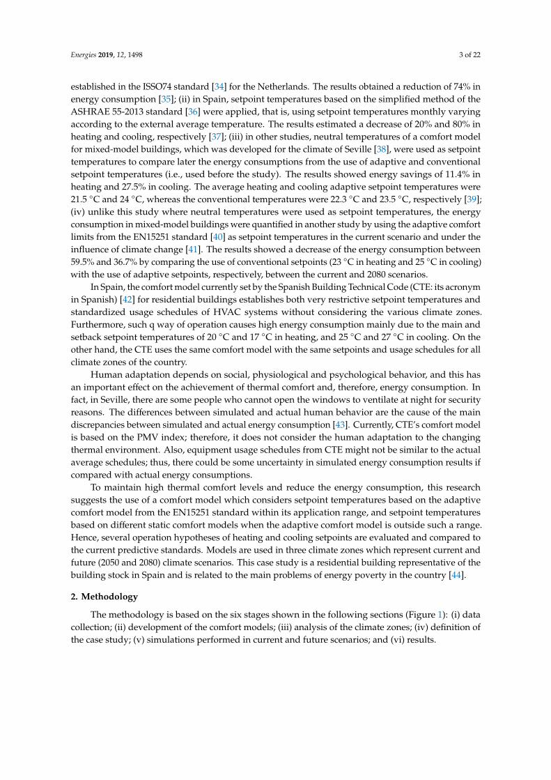
The methodology is based on the six stages shown in the following sections (Figure 1): (i) datacollection; (ii) development of the comfort models; (iii) analysis of the climate zones; (iv) definition ofthe case study; (v) simulations performed in current and future scenarios; and (vi) results.
Energies 2019, 12, 1498 4 of 22Energies 2019, 12, x 4 of 22
Figure 1. Methodology flowchart.
2.1. Data Collection
To study the potential of the adaptive comfort model, it is required to establish the setpoint
temperatures which fix the limits of the internal temperatures from which air‐conditioning systems
in the dwelling start to work.
The setpoint temperatures in the static model are set according to the CTE [42]. However, the
procedure to obtain the adaptive setpoint temperatures is more complex. The adaptive setpoint
temperatures correspond with the adaptive comfort limits from the EN15251 standard [40], which in
turn depend on the running mean outdoor temperature. The running mean outdoor temperature is
calculated by using Equation (1).
Ɵ Ɵ 0.8 ∗ Ɵ 0.6 ∗ Ɵ 0.5 ∗ Ɵ 0.4 ∗ Ɵ 0.3 ∗ Ɵ 0.2 ∗ Ɵ 3.8⁄ , (1)
where ƟEd−1 is the daily average external air temperature of the previous day, ƟEd−2 is the daily average external air temperature of two days before, and so on.
The EN15251 standard establishes different categories (Table 1) in which the level of expectation
of the thermal ambient of the occupant is determined. Moreover, the extent of the comfort range
depends on such categories. In this case study, as it is an existing building, category III is the
appropriate category. For such a category, the adaptive comfort limits are calculated by Equations (2)
and (3).
Ɵ 0.33 Ɵ 18.8 4, (2)
Ɵ 0.33 Ɵ 18.8 4, (3)
where Ɵ is the temperature of the upper limit, Ɵ is the temperature of the lower limit, Ɵ is the internal operative temperature, and Ɵ is the average external working temperature.
Figure 1. Methodology flowchart.
2.1. Data Collection
To study the potential of the adaptive comfort model, it is required to establish the setpointtemperatures which fix the limits of the internal temperatures from which air-conditioning systems inthe dwelling start to work.
The setpoint temperatures in the static model are set according to the CTE [42]. However, theprocedure to obtain the adaptive setpoint temperatures is more complex. The adaptive setpointtemperatures correspond with the adaptive comfort limits from the EN15251 standard [40], which inturn depend on the running mean outdoor temperature. The running mean outdoor temperature iscalculated by using Equation (1).
θrm = (θed−1 + 0.8 ∗ θed−2 + 0.6 ∗ θed−3 + 0.5 ∗ θed−4 + 0.4 ∗ θed−5 + 0.3 ∗ θed−6 + 0.2 ∗ θed−7)/3.8, (1)
where θEd−1 is the daily average external air temperature of the previous day, θEd−2 is the daily averageexternal air temperature of two days before, and so on.
The EN15251 standard establishes different categories (Table 1) in which the level of expectation ofthe thermal ambient of the occupant is determined. Moreover, the extent of the comfort range dependson such categories. In this case study, as it is an existing building, category III is the appropriatecategory. For such a category, the adaptive comfort limits are calculated by Equations (2) and (3).
θi max = 0.33× θrm + 18.8 + 4, (2)
θi min = 0.33× θrm + 18.8− 4, (3)
where θi max is the temperature of the upper limit, θi min is the temperature of the lower limit, θi is theinternal operative temperature, and θrm is the average external working temperature.

Energies 2019, 12, 1498 5 of 22
Table 1. Expectation categories addressed in EN15251.
Category Detail
I High level of expectation, recommended for spaces occupied by weak and sensitive peoplewith special requirements, such as handicapped, sick, elderly, and very young children.
II Normal level of expectation; it should be used for new and renovated buildings.
III Acceptable and moderate level of expectation; it can be used in existing buildings.
IV Values outside of the criteria of the preceding categories. This category should only beaccepted during a limited part of a year.
This comfort model can be used if some limitations are fulfilled. Regarding the temperature, theaverage external working temperature should be between 10 ◦C and 30 ◦C for the upper comfort limit,and between 15 ◦C and 30 ◦C for the lower limit. It should be considered that the graphic is basedon a database limited for average external working temperatures higher than 25 ◦C. Moreover, theupper comfort limit can be extended to around 3.5 ◦C by increasing the air speed to 1.5 m/s. On theother hand, regarding the occupant, the metabolic activity should be between 1.0 and 1.3 met, and thelevel of clo between 0.5 and 1. Such a comfort model considers the opportunities of the occupant’sadaptation to the thermal ambient. Therefore, it can be applied to buildings where the opening andclosing of windows is possible, as well as where occupants can adapt their clothing to their needs.
2.2. Models
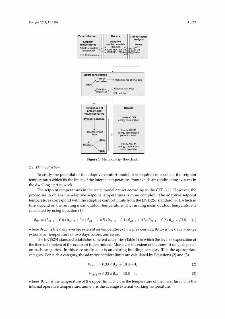
Four different comfort models were suggested for this study: (a) a static model based on thesetpoints of the CTE, and (b) three adaptive models: OUT-CTE, OUT-SEN15251, and OUT-AEN15251.In the adaptive models, adaptive heating setpoint temperatures (AHST) and adaptive cooling setpointtemperatures (ACST) are used, which correspond with the comfort limits for Category III in theEN15251 standard when the comfort model is applied. Currently, the use of the static model based onthe setpoints of the CTE generates high energy consumptions due to the use of very restrictive setpointtemperatures. Thus, the use of the adaptive models OUT-CTE, OUT-SEN15251, and OUT-AEN15251could reduce the energy consumption and maintain high comfort levels. When the adaptive thermalcomfort model cannot be applied, the following configurations are used: (i) for OUT-CTE, the setpointtemperatures of the CTE are used; (ii) for OUT-SEN15251, the static setpoint temperatures of theEN15251 standard are used (they are included in Table A.3 of the EN15251 standard (i.e., when therunning mean outdoor temperature is lower than 10 ◦C, heating and cooling setpoints are 18 ◦C and25 ◦C, respectively, and when the running mean outdoor temperature is higher than 30 ◦C, setpoints are22 ◦C and 27 ◦C, respectively); and (iii) for OUT-AEN15251, maximum and minimum comfort limitsof the EN15251 standard are used as static setpoint temperatures in its adaptive model, extendinghorizontally the maximum and minimum comfort limits (i.e., the internal operative temperatureswhich correspond to average external working temperatures of 30 ◦C for the upper limit, and 15 ◦C forthe lower limit). Table 2 and Figure 2 show such setpoint temperatures. In addition, the values of thesetpoint temperatures vary in schedule ranges (12:00–7:00 a.m., 8:00 a.m.–3:00 p.m., and 4:00–11:00 p.m.)in the CTE static model. To make representative comparisons, such values also varied in the OUT-CTEmodel. Also, it is advisable to consider that the working schedule of the air-conditioning equipmentset in the CTE was used to establish a coherent comparison between the static model set in the CTE andthe adaptive models proposed. In this way, the cooling mode works from June to September, between4:00 p.m. and 7:00 a.m., whereas the heating mode works from January to May and from October toDecember throughout the day.
Energies 2019, 12, 1498 6 of 22
Table 2. Setpoint temperatures used in each model.
Model Standard Limit Range
Setpoint Temperature (◦C)
January–May June–September October–December
24–7 8–15 16–23 24–7 8–15 16–23 24–7 8–15 16–23
Static model CTEUpperlimit all - - - 27 - 25 - - -
Lowerlimit all 17 20 20 - - - 17 20 20
Adaptivemodel
OUT-CTE
EN15251Cat.III
CTE
Upperlimit
(ACST)
θrm < 10 ◦C - - - 27 - 25 - - -10 ◦C ≤ θrm < 30 ◦C - - - (1) - (1) - - -
θrm > 30 ◦C - - - 27 - 25 - - -
Lowerlimit
(AHST)
θrm < 15 ◦C 17 20 20 - - - 17 20 2015 ◦C ≤ θrm ≤ 30 ◦C (2) - - - (2)
θrm > 30 ◦C 17 20 20 - - - 17 20 20
Adaptivemodel
OUT-SEN15251
EN15251Cat. III
Upperlimit
(ACST)
θrm < 10 ◦C - - - 25 - 25 - - -10 ◦C ≤ θrm < 30 ◦C - - - (1) - (1) - - -
θrm > 30 ◦C - - - 27 - 27 - - -
Lowerlimit
(AHST)
θrm < 15 ◦C 18 - - - 1815 ◦C ≤ θrm ≤ 30 ◦C (2) - - - (2)
θrm > 30 ◦C 22 - - - 22
Adaptivemodel
OUT-AEN15251
EN15251Cat. III
Upperlimit
(ACST)
θrm < 10 ◦C - - - 26.10 - 26.10 - - -10 ◦C ≤ θrm < 30 ◦C - - - (1) - (1) - - -
θrm > 30 ◦C - - - 32.70 - 32.70 - - -
Lowerlimit
(AHST)
θrm < 15 ◦C 19.75 - - - 19.7515 ◦C ≤ θrm ≤ 30 ◦C (2) - - - (2)
θrm > 30 ◦C 24.70 - - - 24.70
Notes: ACST: adaptive cooling setpoint temperature; AHST: adaptive heating setpoint temperature; CTE: SpanishBuilding Technical Code. (1) 0.33× θrm + 18.8 + 4; (2) 0.33× θrm + 18.8− 4.
Energies 2019, 12, x 6 of 22
Table 2. Setpoint temperatures used in each model.
Model Standard Limit Range
Setpoint Temperature (°C)
January–May June–September October–December
24–7 8–15 16–23 24–7 8–15 16–23 24–7 8–15 16–23
Static model CTE Upper limit all ‐ ‐ ‐ 27 ‐ 25 ‐ ‐ ‐
Lower limit all 17 20 20 ‐ ‐ ‐ 17 20 20
Adaptive model
OUT‐CTE
EN15251
Cat. III
CTE
Upper limit (ACST)
Ɵ < 10 °C ‐ ‐ ‐ 27 ‐ 25 ‐ ‐ ‐
10 °C ≤ Ɵ < 30 °C ‐ ‐ ‐ (1) ‐ (1) ‐ ‐ ‐
Ɵ > 30 °C ‐ ‐ ‐ 27 ‐ 25 ‐ ‐ ‐
Lower limit (AHST)
Ɵ < 15 °C 17 20 20 ‐ ‐ ‐ 17 20 20
15 °C ≤ Ɵ ≤ 30 °C (2) ‐ ‐ ‐ (2)
Ɵ > 30 °C 17 20 20 ‐ ‐ ‐ 17 20 20
Adaptive model
OUT‐SEN15251
EN15251
Cat. III
Upper limit (ACST)
Ɵ < 10 °C ‐ ‐ ‐ 25 ‐ 25 ‐ ‐ ‐
10 °C ≤ Ɵ < 30 °C ‐ ‐ ‐ (1) ‐ (1) ‐ ‐ ‐
Ɵ > 30 °C ‐ ‐ ‐ 27 ‐ 27 ‐ ‐ ‐
Lower limit (AHST)
Ɵ < 15 °C 18 ‐ ‐ ‐ 18
15 °C ≤ Ɵ ≤ 30 °C (2) ‐ ‐ ‐ (2)
Ɵ > 30 °C 22 ‐ ‐ ‐ 22
Adaptive model
OUT‐AEN15251
EN15251
Cat. III
Upper limit (ACST)
Ɵ < 10 °C ‐ ‐ ‐ 26.10 ‐ 26.10 ‐ ‐ ‐
10 °C ≤ Ɵ < 30 °C ‐ ‐ ‐ (1) ‐ (1) ‐ ‐ ‐
Ɵ > 30 °C ‐ ‐ ‐ 32.70 ‐ 32.70 ‐ ‐ ‐
Lower limit (AHST)
Ɵ < 15 °C 19.75 ‐ ‐ ‐ 19.75
15 °C ≤ Ɵ ≤ 30 °C (2) ‐ ‐ ‐ (2)
Ɵ > 30 °C 24.70 ‐ ‐ ‐ 24.70
Notes: ACST: adaptive cooling setpoint temperature; AHST: adaptive heating setpoint temperature;
CTE: Spanish Building Technical Code. (1) 0.33 Ɵ 18.8 4; (2) 0.33 Ɵ 18.8 4.
Figure 2. Setpoints of Spanish Building Technical Code (CTE), OUT‐CTE, OUT‐SEN15251, and OUT‐
AEN15251 models.
The EN15251 adaptive model establishes that the thermal comfort can be achieved by using
ventilation and by the occupant’s adaptation actions if the running mean outdoor temperature fulfils
the conditions of applicability, as well as other conditions related to the HVAC systems and the levels
of both clo and met. If the thermal comfort is not achieved, it would be necessary to activate the
HVAC systems and use setpoint temperatures from the static model of the EN15251 standard.
Figure 2. Setpoints of Spanish Building Technical Code (CTE), OUT-CTE, OUT-SEN15251, andOUT-AEN15251 models.

Energies 2019, 12, 1498 7 of 22
The EN15251 adaptive model establishes that the thermal comfort can be achieved by usingventilation and by the occupant’s adaptation actions if the running mean outdoor temperature fulfilsthe conditions of applicability, as well as other conditions related to the HVAC systems and the levelsof both clo and met. If the thermal comfort is not achieved, it would be necessary to activate the HVACsystems and use setpoint temperatures from the static model of the EN15251 standard. Therefore,when the running mean outdoor temperature is higher than 30 ◦C, the upper and lower limits varyfrom 32.70 ◦C to 27 ◦C, and from 24.70 ◦C to 22 ◦C, respectively. Also, when the running mean outdoortemperature is lower than 10 ◦C, the upper and lower limits vary from 26.10 ◦C to 25 ◦C, and from19.70 ◦C to 18 ◦C, respectively. For this reason, various static models are used when the conditions ofapplicability of the adaptive model are not fulfilled.
2.3. Analysis of Climate Zones
In this paper, the three most representatives climate zones of the Spanish territory set in theCTE DB HE (which is the Spanish Building Technical Code document in relation to energy savings)reference climates were considered [45]: (i) the B4 climate zone, which belongs to class Csa accordingto Köppen–Geiger’s classification [46] (Mediterranean climate, with mild winters and dry and veryhot summers), in which the city of Seville is located; (ii) the D3 climate zone, which belongs to classBSh (cold semi-arid climate, with moderated cold winters and hot summers), in which the city ofMadrid is located; and (iii) the E1 climate zone, which belongs to class Csb (continental Mediterraneanclimate, with mild summers and cold winters), in which the city of Ávila is located. Such climateswere selected with the aim of obtaining results which were extrapolated to other countries with thesame climate zones.
2.4. Definition of the Case Study
The case study was an apartment located on the fourth floor of a residential building of eightfloors, which was built in 1973 with a surface area of 77 m2. The apartment has a living room, a kitchen,a bathroom, and three bedrooms. Figure 3 shows the building and the dwelling studied in red.
Energies 2019, 12, x 7 of 22
Therefore, when the running mean outdoor temperature is higher than 30 °C, the upper and lower
limits vary from 32.70 °C to 27 °C, and from 24.70 °C to 22 °C, respectively. Also, when the running
mean outdoor temperature is lower than 10 °C, the upper and lower limits vary from 26.10 °C to 25
°C, and from 19.70 °C to 18 °C, respectively. For this reason, various static models are used when the
conditions of applicability of the adaptive model are not fulfilled.
2.3. Analysis of Climate Zones
In this paper, the three most representatives climate zones of the Spanish territory set in the CTE
DB HE (which is the Spanish Building Technical Code document in relation to energy savings)
reference climates were considered [45]: (i) the B4 climate zone, which belongs to class Csa according
to Köppen–Geiger’s classification [46] (Mediterranean climate, with mild winters and dry and very
hot summers), in which the city of Seville is located; (ii) the D3 climate zone, which belongs to class
BSh (cold semi‐arid climate, with moderated cold winters and hot summers), in which the city of
Madrid is located; and (iii) the E1 climate zone, which belongs to class Csb (continental
Mediterranean climate, with mild summers and cold winters), in which the city of Ávila is located.
Such climates were selected with the aim of obtaining results which were extrapolated to other
countries with the same climate zones.
2.4. Definition of the Case Study
The case study was an apartment located on the fourth floor of a residential building of eight
floors, which was built in 1973 with a surface area of 77 m2. The apartment has a living room, a
kitchen, a bathroom, and three bedrooms. Figure 3 shows the building and the dwelling studied in
red.
Figure 3. Case study analyzed.
According to data from the National Institute of Statistics (INE: its acronym in Spanish) [12],
5.121 million dwellings (i.e., 27.7% of the total) in Spain have a surface area of 76–90 m2, and most
Figure 3. Case study analyzed.

Energies 2019, 12, 1498 8 of 22
According to data from the National Institute of Statistics (INE: its acronym in Spanish) [12],5.121 million dwellings (i.e., 27.7% of the total) in Spain have a surface area of 76–90 m2, and mostdwellings (1.047 million) were built between 1971 and 1980. The typology of the case study is, therefore,statistically representative.
This dwelling was studied in a previous research paper [32]. In this study, the simulation modelmet the limits of 10% and 30% on Mean Bias Error (MBE) and Coefficient of Variation of the RootSquare Mean Error (CV (RSME)) as per ASHRAE Guideline 14 [47] and, thus, the simulation modelwas validated. The dwelling has a heat pump with an energy efficiency ratio (EER) of 2.00, and with acoefficient of performance (CoP) of 2.10.
Figure 4 shows the constructive characteristics of the building selected. The envelope was usedin many buildings between 1960 and 1980, a period when many residential buildings were built.Also, considering that the incorporation of thermal insulation was not mandatory until 1979 [48], thebuilding selected (which was built in 1973) does not have thermal insulation in the envelope.
Energies 2019, 12, x 8 of 22
dwellings (1.047 million) were built between 1971 and 1980. The typology of the case study is,
therefore, statistically representative.
This dwelling was studied in a previous research paper [32]. In this study, the simulation model
met the limits of 10% and 30% on Mean Bias Error (MBE) and Coefficient of Variation of the Root
Square Mean Error (CV (RSME)) as per ASHRAE Guideline 14 [47] and, thus, the simulation model
was validated. The dwelling has a heat pump with an energy efficiency ratio (EER) of 2.00, and with
a coefficient of performance (CoP) of 2.10.
Figure 4 shows the constructive characteristics of the building selected. The envelope was used
in many buildings between 1960 and 1980, a period when many residential buildings were built. Also,
considering that the incorporation of thermal insulation was not mandatory until 1979 [48], the
building selected (which was built in 1973) does not have thermal insulation in the envelope.
Figure 4. Constructive properties.
The operation schedules used are defined as per CTE for residential use (Figure 5). The
occupation on working days varies throughout the day, reaching 100% from 12:00 to 7:00 a.m. On the
weekend, a total and constant occupation is shown. The use of equipment and lighting reaches 100%
between 8:00 p.m. and 11:00 p.m. Table 3 indicates the maximum values for the internal loads, which
were obtained from the CTE’s reference values to be used in building energy performance
simulations.
During the summer, it is estimated that the inhabitable spaces present a ventilation of four
renovations per hour between 1:00 a.m. and 8:00 a.m. by opening the windows. During the remaining
periods, the minimum volume of external ventilation air for residential use should be applied
according to the CTE. Our case study is a dwelling of three bedrooms, with a minimum volume in
dry rooms of 8 L/s in the main bedroom, 4 L/s in the remaining bedrooms, and 10 L/s in the living
room. In wet rooms, the minimum volume per room should be 8 L/s.
Figure 4. Constructive properties.
The operation schedules used are defined as per CTE for residential use (Figure 5). The occupationon working days varies throughout the day, reaching 100% from 12:00 to 7:00 a.m. On the weekend, atotal and constant occupation is shown. The use of equipment and lighting reaches 100% between8:00 p.m. and 11:00 p.m. Table 3 indicates the maximum values for the internal loads, which wereobtained from the CTE’s reference values to be used in building energy performance simulations.
During the summer, it is estimated that the inhabitable spaces present a ventilation of fourrenovations per hour between 1:00 a.m. and 8:00 a.m. by opening the windows. During the remainingperiods, the minimum volume of external ventilation air for residential use should be applied accordingto the CTE. Our case study is a dwelling of three bedrooms, with a minimum volume in dry rooms of8 L/s in the main bedroom, 4 L/s in the remaining bedrooms, and 10 L/s in the living room. In wetrooms, the minimum volume per room should be 8 L/s.

Energies 2019, 12, 1498 9 of 22
Energies 2019, 12, x 9 of 22
Table 3. Internal loads.
Internal Loads W/m2 at 100%
Sensible occupancy 2.15
Latent occupancy 1.36
Lighting 4.40
Equipment 4.40
Figure 5. Operative schedules.
2.5. Simulation in Current and Future Scenarios
Simulations were performed using DesignBuilder software because it includes EnergyPlus (a
calculation engine), which develops advanced dynamic simulations by using schedule weather data
files of each climate zone under study. Figure 6 shows the model developed in DesignBuilder, in
which the environment of the building (a) and upper and lower floors of the dwelling under study
(b) were modeled to obtain accurate results. The dwelling was modeled by in situ measurements,
developing a very real envelope of façades and gaps (according to the constructive characteristics in
Figure 4) and considering the operation hypothesis and the internal loads set in the CTE (according
to Figure 5 and Table 3). Moreover, the adaptive setpoint temperatures included in Table 2 were
applied by using Compact Schedules.
Figure 6. (a) Thermal model; (b) dwellings analyzed.
In this study, the application of adaptive setpoints in future climate scenarios was also evaluated.
For this purpose, the CCWorldWeatherGen tool of the United Kingdom (UK) Met Office Hadley
Centre Coupled Model 3 (HadCM3) was used because it generates weather files which are adapted
to the climate change of any place in the world, as well as files compatible with most building
performance simulation programs [49]. The morphing of the three current climate files (B4, D3 E1)
was carried out for the A2 scenario of greenhouse gas emissions, which is considered medium–high
by the Intergovernmental Panel on Climate Change (IPCC), resulting in climate scenarios files for
2050 and 2080. By using this method, files of the Energy Plus Weather (EPW) climate of the place in
Figure 5. Operative schedules.
Table 3. Internal loads.
Internal Loads W/m2 at 100%
Sensible occupancy 2.15Latent occupancy 1.36
Lighting 4.40Equipment 4.40
2.5. Simulation in Current and Future Scenarios
Simulations were performed using DesignBuilder software because it includes EnergyPlus(a calculation engine), which develops advanced dynamic simulations by using schedule weather datafiles of each climate zone under study. Figure 6 shows the model developed in DesignBuilder, in whichthe environment of the building (a) and upper and lower floors of the dwelling under study (b) weremodeled to obtain accurate results. The dwelling was modeled by in situ measurements, developing avery real envelope of façades and gaps (according to the constructive characteristics in Figure 4) andconsidering the operation hypothesis and the internal loads set in the CTE (according to Figure 5 andTable 3). Moreover, the adaptive setpoint temperatures included in Table 2 were applied by usingCompact Schedules.
Energies 2019, 12, x 9 of 22
Table 3. Internal loads.
Internal Loads W/m2 at 100%
Sensible occupancy 2.15
Latent occupancy 1.36
Lighting 4.40
Equipment 4.40
Figure 5. Operative schedules.
2.5. Simulation in Current and Future Scenarios
Simulations were performed using DesignBuilder software because it includes EnergyPlus (a
calculation engine), which develops advanced dynamic simulations by using schedule weather data
files of each climate zone under study. Figure 6 shows the model developed in DesignBuilder, in
which the environment of the building (a) and upper and lower floors of the dwelling under study
(b) were modeled to obtain accurate results. The dwelling was modeled by in situ measurements,
developing a very real envelope of façades and gaps (according to the constructive characteristics in
Figure 4) and considering the operation hypothesis and the internal loads set in the CTE (according
to Figure 5 and Table 3). Moreover, the adaptive setpoint temperatures included in Table 2 were
applied by using Compact Schedules.
Figure 6. (a) Thermal model; (b) dwellings analyzed.
In this study, the application of adaptive setpoints in future climate scenarios was also evaluated.
For this purpose, the CCWorldWeatherGen tool of the United Kingdom (UK) Met Office Hadley
Centre Coupled Model 3 (HadCM3) was used because it generates weather files which are adapted
to the climate change of any place in the world, as well as files compatible with most building
performance simulation programs [49]. The morphing of the three current climate files (B4, D3 E1)
was carried out for the A2 scenario of greenhouse gas emissions, which is considered medium–high
by the Intergovernmental Panel on Climate Change (IPCC), resulting in climate scenarios files for
2050 and 2080. By using this method, files of the Energy Plus Weather (EPW) climate of the place in
Figure 6. (a) Thermal model; (b) dwellings analyzed.
In this study, the application of adaptive setpoints in future climate scenarios was also evaluated.For this purpose, the CCWorldWeatherGen tool of the United Kingdom (UK) Met Office Hadley CentreCoupled Model 3 (HadCM3) was used because it generates weather files which are adapted to theclimate change of any place in the world, as well as files compatible with most building performancesimulation programs [49]. The morphing of the three current climate files (B4, D3 E1) was carriedout for the A2 scenario of greenhouse gas emissions, which is considered medium–high by the

Energies 2019, 12, 1498 10 of 22
Intergovernmental Panel on Climate Change (IPCC), resulting in climate scenarios files for 2050 and2080. By using this method, files of the Energy Plus Weather (EPW) climate of the place in questionwere obtained, and then the morphing process was carried out with projections of the GMC (generalcirculation model). In such a morphing process, the A2a, A2b, and A2c guidelines of the HadCM3model were combined.
One of the advantages of the morphing process is the change of monthly mean climate values toshow future variations, while maintaining the underlying characteristics of the current climate. Inthis way, the coherence with historic data is maintained, and buildings in current and future climatescan be directly compared. Regarding the disadvantages, some variables are produced independently;hence, the relationship between them and the new climate files could not be the same, as in the historicfiles [18]. In addition, this method has the following limitations: (i) it should be considered that theresolution of HadCM3 is mainly used on a global scale; (ii) the HadCM3 model covers a finite grid pointmodel covering an area of 2.5◦ latitude by 3.75◦ longitude, with a resolution of around 300 × 300 km2
in the whole world; (iii) this method does not consider the microclimate effects typical of the cities(e.g., urban heating island) because the weather stations, which record data to be used for generatingclimate files, are generally located in the outskirts of the cities; and (iv) this method does not considerextraordinary natural phenomena because it only estimates future tendencies from average values.
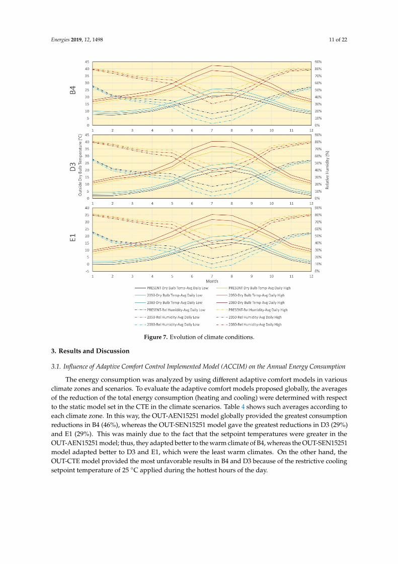
Figure 7 shows the increase in the average temperature of daily minimum and maximumtemperatures, and the variation of the relative humidity due to climate change. The annual averagetemperature increases in B4, D3, and E1 scenarios from 18.7 ◦C to 22.5 ◦C, from 14.7 ◦C to 18.5 ◦C, andfrom 11.6 ◦C to 15.4 ◦C, respectively. However, as can be seen in such three climate zones, the effectsof global warming do not equally influence throughout the year, as the increase in temperature andthe respective decrease in humidity are less in cold months than in warm months. January showsan increase in the average minimum and maximum temperatures of 2.3 ◦C and 2.5 ◦C, respectively,whereas in July there are increases of 5.2 ◦C and 7.4 ◦C, respectively. Regarding the variation of therelative humidity, the variation in the average maximum and minimum temperatures is the samethroughout the year, except in July. While in January, both minimum and maximum averages aredecreased by 2%, the average of the minimum temperatures is reduced by 13.8% and the average ofthe maximum temperatures is reduced by 15.9% in July.
The comfort model set in the EN15251 standard allows the comfort levels to be evaluated only inthe current scenario. In this way, as there are no comfort models available for future scenarios, thecomfort model of the EN15251 standard was used for the climate scenarios of 2050 and 2080. Thiscould imply a limitation because the acceptability and comfort ranges could change as the humanbeings adapt to the increase in temperature. Thus, the calculation of the comfort levels and theadaptive energy consumption is limited because the adaptation of the temperature increase was notconsidered. However, it is possible that the potential of energy saving grows. This is due to thefact that, if the adaptation to future scenarios is considered, human beings might consider highertemperatures acceptable; thus, the adaptive setpoint temperatures could be higher than those of thecurrent scenario [41].
Energies 2019, 12, 1498 11 of 22
Energies 2019, 12, x 11 of 22
Figure 7. Evolution of climate conditions.
The comfort model set in the EN15251 standard allows the comfort levels to be evaluated only
in the current scenario. In this way, as there are no comfort models available for future scenarios, the
comfort model of the EN15251 standard was used for the climate scenarios of 2050 and 2080. This
could imply a limitation because the acceptability and comfort ranges could change as the human
beings adapt to the increase in temperature. Thus, the calculation of the comfort levels and the
adaptive energy consumption is limited because the adaptation of the temperature increase was not
considered. However, it is possible that the potential of energy saving grows. This is due to the fact
that, if the adaptation to future scenarios is considered, human beings might consider higher
temperatures acceptable; thus, the adaptive setpoint temperatures could be higher than those of the
current scenario [41].
3. Results and Discussion
3.1. Influence of Adaptive Comfort Control Implemented Model (ACCIM) on the Annual Energy
Consumption
The energy consumption was analyzed by using different adaptive comfort models in various
climate zones and scenarios. To evaluate the adaptive comfort models proposed globally, the
averages of the reduction of the total energy consumption (heating and cooling) were determined
with respect to the static model set in the CTE in the climate scenarios. Table 4 shows such averages
according to each climate zone. In this way, the OUT‐AEN15251 model globally provided the greatest
Figure 7. Evolution of climate conditions.
3. Results and Discussion
3.1. Influence of Adaptive Comfort Control Implemented Model (ACCIM) on the Annual Energy Consumption
The energy consumption was analyzed by using different adaptive comfort models in variousclimate zones and scenarios. To evaluate the adaptive comfort models proposed globally, the averagesof the reduction of the total energy consumption (heating and cooling) were determined with respectto the static model set in the CTE in the climate scenarios. Table 4 shows such averages according toeach climate zone. In this way, the OUT-AEN15251 model globally provided the greatest consumptionreductions in B4 (46%), whereas the OUT-SEN15251 model gave the greatest reductions in D3 (29%)and E1 (29%). This was mainly due to the fact that the setpoint temperatures were greater in theOUT-AEN15251 model; thus, they adapted better to the warm climate of B4, whereas the OUT-SEN15251model adapted better to D3 and E1, which were the least warm climates. On the other hand, theOUT-CTE model provided the most unfavorable results in B4 and D3 because of the restrictive coolingsetpoint temperature of 25 ◦C applied during the hottest hours of the day.

Energies 2019, 12, 1498 12 of 22
Table 4. Reduction of the total energy consumption with respect to the CTE.
ZoneModels
OUT-CTE OUT-SEN15251 OUT-AEN15251
B4 23% 33% 46%
D3 19% 29% 25%
E1 17% 29% 10%
Nevertheless, such results were analyzed in detail (Figure 8 and Table 5), including those ofthe static model according to the CTE. The results obtained from the heating, cooling, and totalconsumption were analyzed, as well as the results according to the climate zone. Moreover, thepercentages of reduction in energy consumption with respect to the static model of the CTE are shown.
Regarding the heating consumption, the greatest total energy consumption was in theCTE-AEN15251 model in the three climate zones, both in current and future scenarios, mainlydue to the fact that, outside the applicability limits, the lower limit of temperature was 19.75 ◦C andthat such a model continuously had the highest heating setpoint temperature. B4 presented the lowestheating consumption because the temperatures in this zone were closer to such a limit.
As for cooling, the greatest energy consumption was obtained by using static setpoints (CTEmodel) and the lowest energy consumption was obtained with the OUT-AEN15251 model because ofthe setpoint temperatures used: the static model of the CTE establishes the setpoint temperature of25 ◦C in daytime hours, whereas the OUT-AEN15251 model establishes 32.70 ◦C as the highest. In thiscase, B4 presented the greatest cooling consumption because it had the highest temperatures.Energies 2019, 12, x 14 of 22
Figure 8. Global energy consumption for the different models and scenarios considered.
With respect to the total consumption for the current scenario, the three climate zones coincided
in that the OUT‐SEN15251 model obtained the least consumption, with reductions of 50%, 36%, and
22% for B4, D3, and E1, respectively. In the context of climate change, the ideal application model to
obtain the lowest energy consumption depended on the climate zone; therefore, each zone was
separately studied in the various climate scenarios.
B4 obtained a lower consumption with the OUT‐SEN15251 model in the current scenario, which
reached a percentage reduction of 50%. However, for 2050 and 2080, such a zone (B4) benefited by
applying the OUT‐AEN15251 model, which had a higher upper limit of temperature, obtaining
reductions of 48% and 44%, respectively.
A similar behavior was found in D3. The lowest consumption was obtained in the current and
2050 scenarios by using the OUT‐SEN15251 model, achieving reductions of 36% and 29%,
respectively. Such scenarios have external temperatures which cause a heating consumption; thus,
having a lower temperature limit as high as that presented by the OUT‐AEN15251 model would be
negative. On the contrary, the OUT‐AEN15251 model had the lowest consumption for 2080, with a
reduction of 31% because of the considerable increase of temperatures.
In E1, the model which obtained the lowest energy consumption was the OUT‐SEN15251 model
for the three climate scenarios, reducing the energy consumption by 22%, 30%, and 34% for the
current, 2050, and 2080 scenarios, respectively. Such a zone presented the lowest temperatures; hence,
models with setpoints as high as the OUT‐AEN15251 model are not advisable. Even considering
future climate scenarios in which the temperature increases considerably, heating was significantly
required in such a zone. This aspect can be seen in the increasing tendency of the percentages of
reduction in future climate scenarios because heating was always greater than cooling.
The reduction on energy consumption in each climatic zone is related to the change of setpoint
temperatures and climate change. However, it must be understood that there are some other factors
influencing the energy consumption in future scenarios, such as the improvement of the EER or CoP
values, or the incorporation of new air‐conditioning systems in dwellings. Another limitation is that
human behavior could be expected to change in future scenarios. Given the difficulty of this
Figure 8. Global energy consumption for the different models and scenarios considered.

Energies 2019, 12, 1498 13 of 22
Table 5. Reduction of the consumption of the adaptive models.
Climatic Zone ScenarioCTE OUT-CTE OUT-SEN15251 OUT-AEN15251
kWh/m2·Year kWh/m2·Year Reduction (%) kWh/m2·Year Reduction (%) kWh/m2·Year Reduction (%)
B4
CurrentCooling 3652.45 1682.26 54% 1561.01 57% 1065.81 71%Heating 1504.85 1484.04 1% 1040.56 31% 1727.15 −15%
Total 5157.30 3166.30 39% 2601.57 50% 2792.96 46%
2050Cooling 5196.55 3904.71 25% 3626.22 30% 2052.95 60%Heating 1060.49 1078.04 −2% 695.50 34% 1220.57 −15%
Total 6257.04 4982.75 20% 4321.72 31% 3273.52 48%
2080Cooling 7116.07 6351.04 11% 5962.58 16% 3616.59 49%Heating 687.07 673.17 2% 385.79 44% 759.12 −10%
Total 7803.14 7024.22 10% 6348.36 19% 4375.71 44%
D3
CurrentCooling 2773.06 745.89 73% 722.83 74% 640.52 77%Heating 5105.23 5113.53 0% 4323.58 15% 5778.52 −13%
Total 7878.28 5859.42 26% 5046.41 36% 6419.04 19%
2050Cooling 4150.70 2595.82 37% 2395.47 42% 1399.97 66%Heating 4273.92 4260.92 0% 3556.26 17% 4851.81 −14%
Total 8424.62 6856.73 19% 5951.73 29% 6251.78 26%
2080Cooling 5931.86 4762.16 20% 4448.74 25% 2624.20 56%Heating 3368.92 3371.96 0% 2729.79 19% 3835.79 −14%
Total 9300.78 8134.12 13% 7178.54 23% 6459.99 31%
E1
CurrentCooling 844.63 37.54 96% 37.72 96% 37.72 96%Heating 7005.40 7037.78 0% 6079.29 13% 7864.73 −12%
Total 7850.02 7075.32 10% 6117.01 22% 7902.45 −1%
2050Cooling 1738.24 229.21 87% 228.41 87% 228.41 87%Heating 6010.11 6038.63 0% 5159.90 14% 6785.03 −13%
Total 7748.36 6267.84 19% 5388.31 30% 7013.44 9%
2080Cooling 3046.99 1174.32 61% 1090.36 64% 742.19 76%Heating 4863.72 4876.70 0% 4117.06 15% 5510.47 −13%
Total 7910.71 6051.02 24% 5207.42 34% 6252.65 21%

Energies 2019, 12, 1498 14 of 22
With respect to the total consumption for the current scenario, the three climate zones coincidedin that the OUT-SEN15251 model obtained the least consumption, with reductions of 50%, 36%, and22% for B4, D3, and E1, respectively. In the context of climate change, the ideal application modelto obtain the lowest energy consumption depended on the climate zone; therefore, each zone wasseparately studied in the various climate scenarios.
B4 obtained a lower consumption with the OUT-SEN15251 model in the current scenario, whichreached a percentage reduction of 50%. However, for 2050 and 2080, such a zone (B4) benefitedby applying the OUT-AEN15251 model, which had a higher upper limit of temperature, obtainingreductions of 48% and 44%, respectively.
A similar behavior was found in D3. The lowest consumption was obtained in the current and2050 scenarios by using the OUT-SEN15251 model, achieving reductions of 36% and 29%, respectively.Such scenarios have external temperatures which cause a heating consumption; thus, having a lowertemperature limit as high as that presented by the OUT-AEN15251 model would be negative. On thecontrary, the OUT-AEN15251 model had the lowest consumption for 2080, with a reduction of 31%because of the considerable increase of temperatures.
In E1, the model which obtained the lowest energy consumption was the OUT-SEN15251 modelfor the three climate scenarios, reducing the energy consumption by 22%, 30%, and 34% for the current,2050, and 2080 scenarios, respectively. Such a zone presented the lowest temperatures; hence, modelswith setpoints as high as the OUT-AEN15251 model are not advisable. Even considering future climatescenarios in which the temperature increases considerably, heating was significantly required in sucha zone. This aspect can be seen in the increasing tendency of the percentages of reduction in futureclimate scenarios because heating was always greater than cooling.
The reduction on energy consumption in each climatic zone is related to the change of setpointtemperatures and climate change. However, it must be understood that there are some other factorsinfluencing the energy consumption in future scenarios, such as the improvement of the EER or CoPvalues, or the incorporation of new air-conditioning systems in dwellings. Another limitation is thathuman behavior could be expected to change in future scenarios. Given the difficulty of this prediction,human behavior in the current scenario was used in future scenarios as well; thus, this could lead tosome uncertainty in the results of energy consumption.
3.2. Influence of ACCIM on the Schedule Energy Consumption: Current Scenario
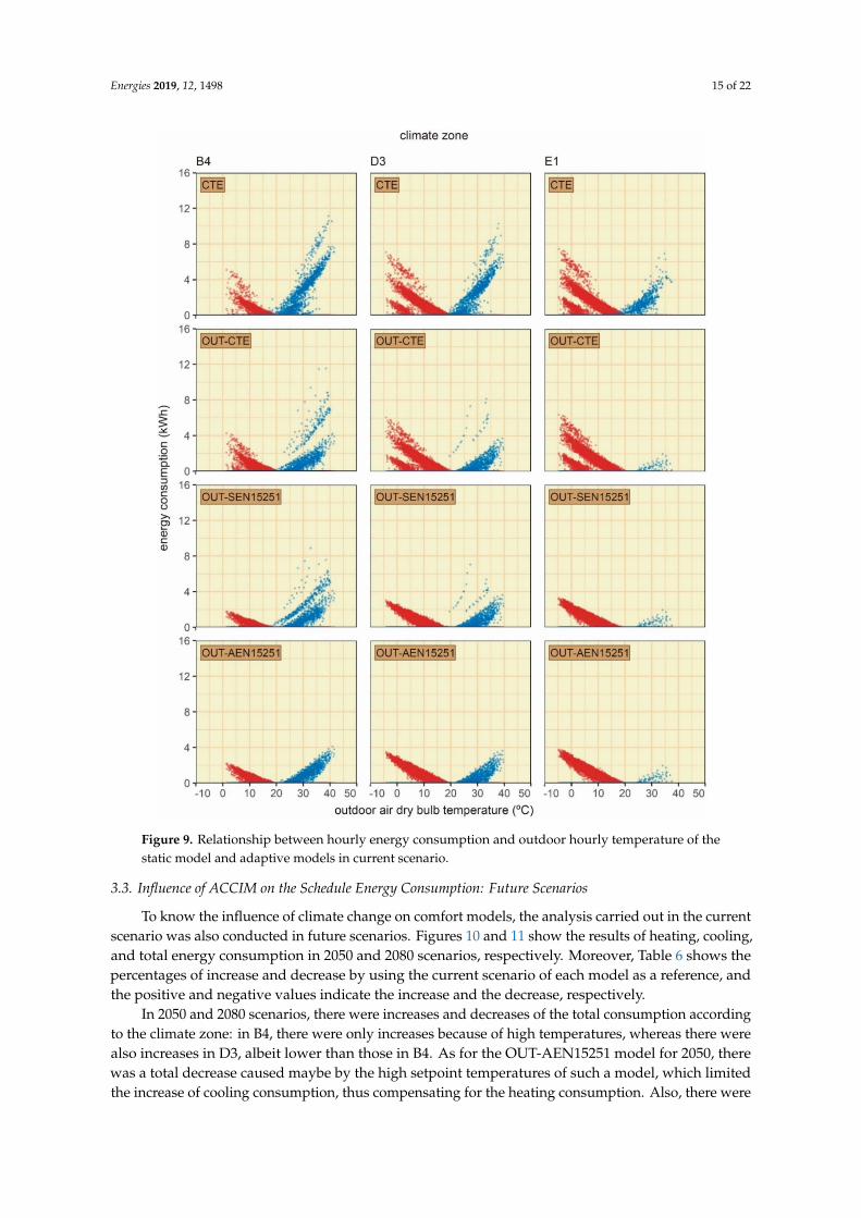
Figure 9 shows the hourly values of heating and cooling energy consumption. A different tendencybetween the static model and the adaptive models was found. In the analysis of the static model (CTE)of the three zones studied, B4 was the zone with the greatest summer climate severity. The highestpick of cooling consumption was, therefore, found in this zone by using such a model, reaching aschedule consumption of up to 11 kWh. In D3 and E1, the maximum cooling values oscillated between7 and 4 kWh, although 10 and 7 kWh were reached in some hours. On the contrary, the highest heatingconsumption was produced in E1, exceeding 7 kWh.
The reduction of such maximum consumption values produced in the adaptive models in contrastto the CTE static model was analyzed. Considering that the consumptions between OUT-CTE,OUT-AEN15251, and OUT-SEN15251 were the same when the adaptive model was applied, thevariations between the graphics sharing climate scenario and zone belonged to those hours when thestatic models were applied. As for CTE and OUT-CTE, those intermediate zones (in which there wasno heating or cooling energy consumption) belonged to the change of the main and setback setpointtemperatures: (i) 20 ◦C and 17 ◦C for heating; and (ii) 27 ◦C and 25 ◦C for cooling.
Regarding the cooling energy consumption, there was a reduction in B4 in adaptive models withrespect to the CTE model. In this way, the heating consumption had a similar behavior in this climatezone. For D3, the schedule values of heating and cooling were slightly lower than those of E1 and B4,respectively. However, Table 5 shows that the total consumption was equal or lower than that of E1,as well as higher than B4.
Energies 2019, 12, 1498 15 of 22
Energies 2019, 12, x 15 of 22
prediction, human behavior in the current scenario was used in future scenarios as well; thus, this
could lead to some uncertainty in the results of energy consumption.
3.2. Influence of ACCIM on the Schedule Energy Consumption: Current Scenario
Figure 9 shows the hourly values of heating and cooling energy consumption. A different
tendency between the static model and the adaptive models was found. In the analysis of the static
model (CTE) of the three zones studied, B4 was the zone with the greatest summer climate severity.
The highest pick of cooling consumption was, therefore, found in this zone by using such a model,
reaching a schedule consumption of up to 11 kWh. In D3 and E1, the maximum cooling values
oscillated between 7 and 4 kWh, although 10 and 7 kWh were reached in some hours. On the contrary,
the highest heating consumption was produced in E1, exceeding 7 kWh.
Figure 9. Relationship between hourly energy consumption and outdoor hourly temperature of the
static model and adaptive models in current scenario.
The reduction of such maximum consumption values produced in the adaptive models in
contrast to the CTE static model was analyzed. Considering that the consumptions between OUT‐
Figure 9. Relationship between hourly energy consumption and outdoor hourly temperature of thestatic model and adaptive models in current scenario.
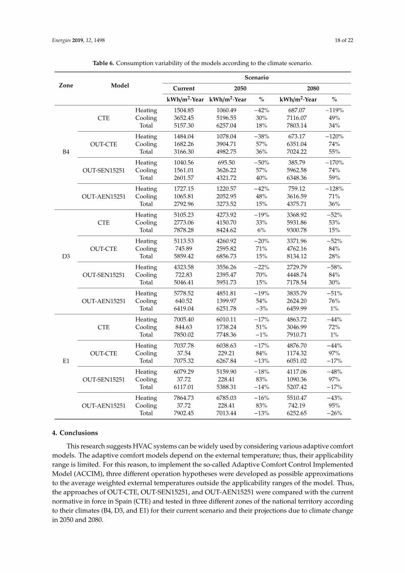
3.3. Influence of ACCIM on the Schedule Energy Consumption: Future Scenarios
To know the influence of climate change on comfort models, the analysis carried out in the currentscenario was also conducted in future scenarios. Figures 10 and 11 show the results of heating, cooling,and total energy consumption in 2050 and 2080 scenarios, respectively. Moreover, Table 6 shows thepercentages of increase and decrease by using the current scenario of each model as a reference, andthe positive and negative values indicate the increase and the decrease, respectively.
In 2050 and 2080 scenarios, there were increases and decreases of the total consumption accordingto the climate zone: in B4, there were only increases because of high temperatures, whereas there werealso increases in D3, albeit lower than those in B4. As for the OUT-AEN15251 model for 2050, therewas a total decrease caused maybe by the high setpoint temperatures of such a model, which limitedthe increase of cooling consumption, thus compensating for the heating consumption. Also, there were

Energies 2019, 12, 1498 16 of 22
decreases in E1, mainly because the variation of heating was greater than that of cooling. As for theCTE model in 2080, there was an increase because of the restrictive cooling setpoint temperature of25 ◦C in daytime hours, which, together with the increase in temperature, implied a higher variation incooling than in heating.
Energies 2019, 12, x 17 of 22
OUT‐AEN15251
Heating 5778.52 4851.81 −19% 3835.79 −51%
Cooling 640.52 1399.97 54% 2624.20 76%
Total 6419.04 6251.78 −3% 6459.99 1%
E1
CTE
Heating 7005.40 6010.11 −17% 4863.72 −44%
Cooling 844.63 1738.24 51% 3046.99 72%
Total 7850.02 7748.36 −1% 7910.71 1%
OUT‐CTE
Heating 7037.78 6038.63 −17% 4876.70 −44%
Cooling 37.54 229.21 84% 1174.32 97%
Total 7075.32 6267.84 −13% 6051.02 −17%
OUT‐SEN15251
Heating 6079.29 5159.90 −18% 4117.06 −48%
Cooling 37.72 228.41 83% 1090.36 97%
Total 6117.01 5388.31 −14% 5207.42 −17%
OUT‐AEN15251
Heating 7864.73 6785.03 −16% 5510.47 −43%
Cooling 37.72 228.41 83% 742.19 95%
Total 7902.45 7013.44 −13% 6252.65 −26%
Figure 10. Relationship between hourly energy consumption and outdoor hourly temperature of the
static model and adaptive models in 2050.
Figure 10. Relationship between hourly energy consumption and outdoor hourly temperature of thestatic model and adaptive models in 2050.
Regarding the maximum schedule consumption values in 2050 (Figure 10), the cooling decreasedin B4 from 14 kWh in CTE and OUT-CTE to around 6 kWh in OUT-AEN15251. Moreover, heatingdecreased from values around 9 kWh in CTE to 3 kWh in OUT-SEN15251 and OUT-AEN15251.
Such values varied in 2080 (Figure 11), as for the cooling consumption in B4, from 16 kWh in CTEand OUT-CTE to around 7 kWh in OUT-AEN15251. As for the heating consumption in E1, valuesvaried from around 7 kWh in CTE to 3 kWh in OUT-SEN15251 and OUT-AEN15251.

Energies 2019, 12, 1498 17 of 22
As for D3, in 2050 and 2080 scenarios, as well as in all comfort models, the maximum values ofheating and cooling consumption were slightly lower than the heating values in E1 and the coolingvalues in B4. In this sense, the highest consumptions were achieved in this zone, except in the totalconsumption of the OUT-AEN15251 model in 2050, which was slightly lower than that in E1, maybebecause of the high heating setpoints of the OUT-AEN15251 model, together with the low temperaturesin E1.Energies 2019, 12, x 18 of 22
Figure 11. Relationship between hourly energy consumption and outdoor hourly temperature of the
static model and adaptive models in 2080.
Regarding the maximum schedule consumption values in 2050 (Figure 10), the cooling
decreased in B4 from 14 kWh in CTE and OUT‐CTE to around 6 kWh in OUT‐AEN15251. Moreover,
heating decreased from values around 9 kWh in CTE to 3 kWh in OUT‐SEN15251 and OUT‐
AEN15251.
Such values varied in 2080 (Figure 11), as for the cooling consumption in B4, from 16 kWh in
CTE and OUT‐CTE to around 7 kWh in OUT‐AEN15251. As for the heating consumption in E1,
values varied from around 7 kWh in CTE to 3 kWh in OUT‐SEN15251 and OUT‐AEN15251.
As for D3, in 2050 and 2080 scenarios, as well as in all comfort models, the maximum values of
heating and cooling consumption were slightly lower than the heating values in E1 and the cooling
Figure 11. Relationship between hourly energy consumption and outdoor hourly temperature of thestatic model and adaptive models in 2080.
Energies 2019, 12, 1498 18 of 22
Table 6. Consumption variability of the models according to the climate scenario.
Zone ModelScenario
Current 2050 2080
kWh/m2·Year kWh/m2·Year % kWh/m2·Year %
B4
CTEHeating 1504.85 1060.49 −42% 687.07 −119%Cooling 3652.45 5196.55 30% 7116.07 49%
Total 5157.30 6257.04 18% 7803.14 34%
OUT-CTEHeating 1484.04 1078.04 −38% 673.17 −120%Cooling 1682.26 3904.71 57% 6351.04 74%
Total 3166.30 4982.75 36% 7024.22 55%
OUT-SEN15251Heating 1040.56 695.50 −50% 385.79 −170%Cooling 1561.01 3626.22 57% 5962.58 74%
Total 2601.57 4321.72 40% 6348.36 59%
OUT-AEN15251Heating 1727.15 1220.57 −42% 759.12 −128%Cooling 1065.81 2052.95 48% 3616.59 71%
Total 2792.96 3273.52 15% 4375.71 36%
D3
CTEHeating 5105.23 4273.92 −19% 3368.92 −52%Cooling 2773.06 4150.70 33% 5931.86 53%
Total 7878.28 8424.62 6% 9300.78 15%
OUT-CTEHeating 5113.53 4260.92 −20% 3371.96 −52%Cooling 745.89 2595.82 71% 4762.16 84%
Total 5859.42 6856.73 15% 8134.12 28%
OUT-SEN15251Heating 4323.58 3556.26 −22% 2729.79 −58%Cooling 722.83 2395.47 70% 4448.74 84%
Total 5046.41 5951.73 15% 7178.54 30%
OUT-AEN15251Heating 5778.52 4851.81 −19% 3835.79 −51%Cooling 640.52 1399.97 54% 2624.20 76%
Total 6419.04 6251.78 −3% 6459.99 1%
E1
CTEHeating 7005.40 6010.11 −17% 4863.72 −44%Cooling 844.63 1738.24 51% 3046.99 72%
Total 7850.02 7748.36 −1% 7910.71 1%
OUT-CTEHeating 7037.78 6038.63 −17% 4876.70 −44%Cooling 37.54 229.21 84% 1174.32 97%
Total 7075.32 6267.84 −13% 6051.02 −17%
OUT-SEN15251Heating 6079.29 5159.90 −18% 4117.06 −48%Cooling 37.72 228.41 83% 1090.36 97%
Total 6117.01 5388.31 −14% 5207.42 −17%
OUT-AEN15251Heating 7864.73 6785.03 −16% 5510.47 −43%Cooling 37.72 228.41 83% 742.19 95%
Total 7902.45 7013.44 −13% 6252.65 −26%
4. Conclusions
This research suggests HVAC systems can be widely used by considering various adaptive comfortmodels. The adaptive comfort models depend on the external temperature; thus, their applicabilityrange is limited. For this reason, to implement the so-called Adaptive Comfort Control ImplementedModel (ACCIM), three different operation hypotheses were developed as possible approximationsto the average weighted external temperatures outside the applicability ranges of the model. Thus,the approaches of OUT-CTE, OUT-SEN15251, and OUT-AEN15251 were compared with the currentnormative in force in Spain (CTE) and tested in three different zones of the national territory accordingto their climates (B4, D3, and E1) for their current scenario and their projections due to climate changein 2050 and 2080.

Energies 2019, 12, 1498 19 of 22
The results demonstrate that the consumption is reduced in different ways by using this predictivemodel, depending on the climate and the hypothesis selected. This variability is also detected in futureprojections (2050 and 2080). Generally, the OUT-SEN15251 and OUT-AEN15251 models presented thebest performance in all climate zones, with the OUT-SEN15251 model obtaining the best behavior inmost of the cases studied for the current scenario. Regarding future scenarios, the models with the bestperformance varied depending on the climate zone: for the warmest zones (B4), the model with thebest performance was OUT-AEN15251; for the coldest climates (E1), the OUT-SEN15251 had the bestperformance; and the model which obtained the lowest consumption for mild climates (D3) in thecurrent scenario and 2050 was OUT-SEN15251, whereas, in 2080, it was OUT-AEN15251.
Nevertheless, although there was a general increase in energy consumption due to global warming(more perceptible in the warmest zones), all the operation hypotheses of the ACCIM models weremore resilient than those of the CTE, even recording total values of consumption which were lower in2080 with respect to the static model in the CTE.
It must be understood that there was some margin of uncertainty in the simulation results.This was mainly due to the lack of information regarding future thermal comfort standards, futurepredictions on human behavior, and future predictions on the improvement of the energy performanceof HVAC systems.
The results obtained in this research provide relevant information to reduce the energy consumptionin buildings. The use of comfort models with adaptive setpoint temperatures significantly reducesthe energy consumption in the existing buildings, both in current and future scenarios. Thus, thecomfort model for the setpoint temperatures used by the normative in force in Spain has limitationsto guarantee an acceptable performance of the existing building stock without damaging users’ lifequality. This aspect is also shown in the normatives of other countries, in which the use of staticsetpoint temperatures is required. The results of this paper can, therefore, be extrapolated to othercountries. Despite this, the applicability of such adaptive models to real case studies constitutes anaspect to be studied; thus, it should be analyzed in further research works.
Finally, more research studies in this field are required to carry out the transition of the staticcomfort models to models which are more related to the external climate conditions and which considerthe users’ climate adaptation. In addition, these research works could support the transition of theSpanish normative to a more sustainable energy consumption without damaging people’s qualityof life.
Author Contributions: All the authors contributed equally to this work. All the authors participated in preparingthe research from the beginning to end, such as establishing the research design, method, and analysis. All theauthors discussed and finalized the analysis results to prepare the manuscript in accordance with the researchprogress. All the authors have read and approved the final manuscript.
Funding: This research received no external funding.
Conflicts of Interest: The authors declare no conflict of interest.
Nomenclature
CodificationAHST Adaptive heating setpoint temperatureACST Adaptive cooling setpoint temperatureCTE Spanish Building Technical CodeB4 Climate zone belonging to class Csa according to Köppen–Geiger’s classification.D3 Climate zone belonging to class BSh according to Köppen–Geiger’s classification.E1 Climate zone belonging to class Csb according to Köppen–Geiger’s classification.HVAC Heating, ventilation, and air conditioningCTE model Static model in the CTEOUT-CTE model Adaptive model of EN15251; when the adaptive model is not applicable, the CTE static model is applied.OUT-SEN15251 model Adaptive model of EN15251; when the adaptive model is not applicable, the EN15251 static model is applied.
OUT-AEN15251 modelAdaptive model of EN15251; when the adaptive model is not applicable, the upper and lower comfort limitsare horizontally extended.
PMV Predicted mean vote

Energies 2019, 12, 1498 20 of 22
References
1. World Wildlife Fund. Living Planet Report 2014: Species and Spaces, People and Places; WWF International:Gland, Switzerland, 2014; Volume 1, ISBN 9780874216561.
2. European Commission. A Roadmap for Moving to a Competitive Low Carbon Economy in 2050; EuropeanCommission: Brussels, Belgium, 2011; pp. 1–15.
3. The United Nations Environment Programme. Building Design and Construction: Forging Resource Efficiencyand Sustainable; The United Nations Environment Programme: Nairobi, Kenya, 2012.
4. Pérez-Lombard, L.; Ortiz, J.; Pout, C. A review on buildings energy consumption information. Energy Build.2008, 40, 394–398. [CrossRef]
5. European Commission. Directive 2002/91/EC of the European Parliament and of the council of 16 December2002 on the energy performance of buildings. Off. J. Eur. Union 2002, 65–71. [CrossRef]
6. European Union. Directive 2010/31/EU of the European Parliament and of the Council of 19 May 2010 on the EnergyPerformance of Buildings; European Union: Brussels, Belgium, 2010; Volume 153, pp. 13–35.
7. Horne, R.; Hayles, C. Towards global benchmarking for sustainable homes: An international comparison ofthe energy performance of housing. J. Hous. Built Environ. 2008, 23, 119–130. [CrossRef]
8. Kurtz, F.; Monzón, M.; López-Mesa, B. Energy and acoustics related obsolescence of social housing of Spain’spost-war in less favoured urban areas. The case of Zaragoza. Inf. La Construcción 2015, 67, m021. [CrossRef]
9. Lowe, R. Technical options and strategies for decarbonizing UK housing. Build. Res. Inf. 2007, 35, 412–425.[CrossRef]
10. Park, K.; Kim, M. Energy Demand Reduction in the Residential Building Sector: A Case Study of Korea.Energies 2017, 10, 1506. [CrossRef]
11. Page, J.; Robinson, D.; Morel, N.; Scartezzini, J.L. A generalised stochastic model for the simulation ofoccupant presence. Energy Build. 2008, 40, 83–98. [CrossRef]
12. Spanish Institute of Statistics Population and Housing Census. Available online: https://www.ine.es/censos2011_datos/cen11_datos_resultados.htm# (accessed on 9 November 2018).
13. Di Pilla, L.; Desogus, G.; Mura, S.; Ricciu, R.; Di Francesco, M. Optimizing the distribution of Italian buildingenergy retrofit incentives with Linear Programming. Energy Build. 2016, 112, 21–27. [CrossRef]
14. Theodoridou, I.; Papadopoulos, A.M.; Hegger, M. A typological classification of the Greek residentialbuilding stock. Energy Build. 2011, 43, 2779–2787. [CrossRef]
15. Pérez-Andreu, V.; Aparicio-Fernández, C.; Martínez-Ibernón, A.; Vivancos, J.L. Impact of climate change onheating and cooling energy demand in a residential building in a Mediterranean climate. Energy 2018, 165,63–74. [CrossRef]
16. Bienvenido-Huertas, D.; Quiñones, J.A.F.; Moyano, J.; Rodríguez-Jiménez, C.E. Patents Analysis of ThermalBridges in Slab Fronts and Their Effect on Energy Demand. Energies 2018, 11, 2222. [CrossRef]
17. Isaac, M.; van Vuuren, D.P. Modeling global residential sector energy demand for heating and air conditioningin the context of climate change. Energy Policy 2009, 37, 507–521. [CrossRef]
18. Cellura, M.; Guarino, F.; Longo, S.; Tumminia, G. Climate change and the building sector: Modelling andenergy implications to an office building in southern Europe. Energy Sustain. Dev. 2018, 45, 46–65. [CrossRef]
19. Intergovernmental Panel on Climate Change Climate change 2014: Synthesis report. Contribution of workinggroups I, II and III to the fifth assessment report of the intergovernmental Panel on climate change. In ClimateChange 2013—The Physical Science Basis; Intergovernmental Panel on Climate Change (Ed.) CambridgeUniversity Press: Cambridge, UK, 2014; pp. 1–30.
20. Karimpour, M.; Belusko, M.; Xing, K.; Boland, J.; Bruno, F. Impact of climate change on the design of energyefficient residential building envelopes. Energy Build. 2015, 87, 142–154. [CrossRef]
21. Kalvelage, K.; Passe, U.; Rabideau, S.; Takle, E.S. Changing climate: The effects on energy demand andhuman comfort. Energy Build. 2014, 76, 373–380. [CrossRef]
22. Rubio-Bellido, C.; Perez-Fargallo, A.; Pulido-Arcas, J.A. Optimization of annual energy demand in officebuildings under the influence of climate change in Chile. Energy 2016, 114, 569–585. [CrossRef]
23. Roaf, S.; Crichton, D.; Nicol, F. Adapting Buildings and Cities for Climate Change: A 21st Century Survival Guide;Routledge: London, UK, 2009.
24. Ren, Z.; Chen, D. Modelling study of the impact of thermal comfort criteria on housing energy use inAustralia. Appl. Energy 2018, 210, 152–166. [CrossRef]

Energies 2019, 12, 1498 21 of 22
25. Tushar, W.; Wang, T.; Lan, L.; Xu, Y.; Withanage, C.; Yuen, C.; Wood, K.L. Policy design for controllingset-point temperature of ACs in shared spaces of buildings. Energy Build. 2017, 134, 105–114. [CrossRef]
26. Hoyt, T.; Arens, E.; Zhang, H. Extending air temperature setpoints: Simulated energy savings and designconsiderations for new and retrofit buildings. Build. Environ. 2014, 88, 89–96. [CrossRef]
27. Wan, K.K.W.; Li, D.H.W.; Lam, J.C. Assessment of climate change impact on building energy use andmitigation measures in subtropical climates. Energy 2011, 36, 1404–1414. [CrossRef]
28. Parry, M.L.; Canziani, O.F.; Palutikof, J.P.; van der Linden, P.J.; Hanson, C.E. Contribution of Working Group IIto the Fourth Assessment Report of the Intergovernmental Panel on Climate Change; Cambridge University Press:Cambridge, UK, 2007.
29. Spyropoulos, G.N.; Balaras, C.A. Energy consumption and the potential of energy savings in Hellenic officebuildings used as bank branches—A case study. Energy Build. 2011, 43, 770–778. [CrossRef]
30. Bienvenido-Huertas, D.; Rubio-Bellido, C.; Pérez-Ordóñez, J.; Martínez-Abella, F. Estimating AdaptiveSetpoint Temperatures Using Weather Stations. Energies 2019, 12, 1197. [CrossRef]
31. Pérez-Fargallo, A.; Pulido-Arcas, J.A.; Rubio-Bellido, C.; Trebilcock, M.; Piderit, B.; Attia, S. Development ofa new adaptive comfort model for low income housing in the central-south of chile. Energy Build. 2018, 178,94–106. [CrossRef]
32. Sánchez-García, D.; Rubio-Bellido, C.; Pulido-Arcas, J.A.; Guevara-García, F.J.; Canivell, J. Adaptive comfortmodels applied to existing Dwellings in Mediterranean climate considering globalwarming. Sustainability2018, 10, 3507. [CrossRef]
33. van der Linden, A.C.; Boerstra, A.C.; Raue, A.K.; Kurvers, S.R.; De Dear, R.J. Adaptive temperature limits: Anew guideline in the Netherlands: A new approach for the assessment of building performance with respectto thermal indoor climate. Energy Build. 2006, 38, 8–17. [CrossRef]
34. Boerstra, A.C.; van Hoof, J.; van Weele, A.M. A new hybrid thermal comfort guideline for the Netherlands:Background and development. Arch. Sci. Rev. 2015, 58, 24–34. [CrossRef]
35. Kramer, R.; van Schijndel, J.; Schellen, H. Dynamic setpoint control for museum indoor climate conditioningintegrating collection and comfort requirements: Development and energy impact for Europe. Build. Environ.2017. [CrossRef]
36. American National Standards Institute/American Society of Heating Refrigerating and Air-ConditioningEngineers (ANSI/ASHRAE). ANSI/ASHRAE Standard 55-2013: Thermal Environmental Conditions for HumanOccupancy; ASHRAE: Atlanta, GA, USA, 2013.
37. Sánchez-Guevara Sánchez, C.; Mavrogianni, A.; Neila González, F.J. On the minimal thermal habitabilityconditions in low income dwellings in Spain for a new definition of fuel poverty. Build. Environ. 2017, 114,344–356. [CrossRef]
38. Barbadilla-Martín, E.; Salmerón Lissén, J.M.; Martín, J.G.; Aparicio-Ruiz, P.; Brotas, L. Field study on adaptivethermal comfort in mixed mode office buildings in southwestern area of Spain. Build. Environ. 2017, 123.[CrossRef]
39. Barbadilla-Martín, E.; Guadix Martín, J.; Salmerón Lissén, J.M.; Sánchez Ramos, J.; Álvarez Domínguez, S.Assessment of thermal comfort and energy savings in a field study on adaptive comfort with application formixed mode offices. Submitt. Energy Build. 2017. [CrossRef]
40. European Committee for Standardization. EN 15251: Indoor Environmental Input Parameters for Design andAssessment of Energy Performance of Buildings—Addressing Indoor Air Quality, Thermal Environment, Lightingand Acoustics; CEN: Brussels, Belgium, 2007; Volume 3, pp. 1–52.
41. Sánchez-García, D.; Rubio-Bellido, C.; del Río, J.J.M.; Pérez-Fargallo, A. Towards the quantification ofenergy demand and consumption through the adaptive comfort approach in mixed mode office buildingsconsidering climate change. Energy Build. 2019, 187, 173–185. [CrossRef]
42. The Government of Spain. Royal Decree 314/2006. Approving the Spanish Technical Building Code CTE-DB-HE-1;The Government of Spain: Madrid, Spain, 2013.
43. Naspi, F.; Arnesano, M.; Stazi, F.; D’Orazio, M.; Revel, G.M. Measuring Occupants’ Behaviour for Buildings’Dynamic Cosimulation. J. Sens. 2018, 2018, 1–17. [CrossRef]
44. Castaño-Rosa, R.; Solís-Guzmán, J.; Marrero, M. A novel Index of Vulnerable Homes: Findings fromapplication in Spain. Indoor Built Environ. 2018. [CrossRef]
45. The Government of Spain. Código Técnico de la Edificación Documento Básico HE Climas de Referencia;The Government of Spain: Madrid, Spain, 2015.

Energies 2019, 12, 1498 22 of 22
46. Rubel, F.; Kottek, M. Observed and projected climate shifts 1901–2100 depicted by world maps of theKöppen-Geiger climate classification. Meteorol. Z. 2010, 19, 135–141. [CrossRef]
47. American National Standards Institute/American Society of Heating Refrigerating and Air-ConditioningEngineers (ANSI/ASHRAE). ASHRAE Guideline 14-2014: Measurement of Energy, Demand, and Water Savings;ASHRAE: Atlanta, GA, USA, 2014; p. 146.
48. Bienvenido-Huertas, D.; Moyano, J.; Rodríguez-Jiménez, C.E.; Marín, D. Applying an artificial neuralnetwork to assess thermal transmittance in walls by means of the thermometric method. Appl. Energy 2019,233–234, 1–14. [CrossRef]
49. Jentsch, M.F.; Bahaj, A.S.; James, P.A.B. Climate Change World Weather Gen, Climate Change World Weather FileGenerator, Version 1.8; Sustainable Energy Research Group: Southampton, UK, 2013.
© 2019 by the authors. Licensee MDPI, Basel, Switzerland. This article is an open accessarticle distributed under the terms and conditions of the Creative Commons Attribution(CC BY) license (http://creativecommons.org/licenses/by/4.0/).