Embed Size (px)
Citation preview

Metodološki zvezki, Vol. 8, No. 1, 2011, 39-55
Adaptive Cluster Sampling
Based on Ranked Sets
Girish Chandra1, Neeraj Tiwari2, and Hukum Chandra3
Abstract
In many surveys, characteristic of interest is sparsely distributed but
highly aggregated; in such situations the adaptive cluster sampling is very
useful. Examples of such populations can be found in fisheries, mineral
investigations (unevenly distributed ore concentrations), animal and plant
populations (rare and endangered species), pollution concentrations and
hot spot investigations, and epidemiology of rare diseases. Ranked Set
Sampling (RSS) is another useful technique for improving the estimates of
mean and variance when the sampling units in a study can be more eas ily
ranked than measured. Under equal and unequal allocation, RSS is found to
be more precise than simple random sampling, as it contains information
about each order statistics. This paper deal with the problem in which the
value of the characteristic under study on the sampled places is low or
negligible but the neighbourhoods of these places may have a few scattered
pockets of the same. We proposed an adaptive cluster sampling theory
based on ranked sets. Different estimators of the population mean are
considered and the proposed design is demonstrated with the help of one
simple example of small populations. The proposed procedure appears to
perform better than the existing procedures of adaptive cluster sampling.
1 Introduction
Thompson (1990) introduced the Adaptive cluster sampling as an efficient
sampling procedure for estimating totals and means of rare and clustered
populations. In adaptive cluster sampling, an initial sample of units is selected by
some ordinary sampling scheme, and, whenever the variable of interest of a unit in
1 Division of GC(R), Tropical Forest Research Institute, Mandla Road, Jabalpur -482021,
India; [email protected]. 2 Department of Statistics, Kumaun University, SSJ Campus Almora, Uttarakhand -263601,
India; [email protected]. 3 Division of Sample Survey, Indian Agricultural Statistics Research Institute, New Delhi -
110012, India; [email protected].

40 Girish Chandra, Neeraj Tiwari, and Hukum Chandra
the sample satisfies a previously specified condition „C‟, neighbouring units are
added to the sample. If any of the newly added units satisfy „C‟, units in their
neighbourhoods are also added until the sample includes all the neighbours of any
unit satisfying the condition „C‟. As noted by Thompson (1990), an adaptive
cluster sampling scheme can be used to investigate a rare contagious disease. First
of all, a simple random sample of people are selected and tested for the disease. If
a person tests positively, then all the friends and contacts of that person are also
tested. If one of the contacts tests positively, then all that person‟s contacts are
tested, and so on. Roesch (1993) used the design for a survey of forest trees.
Thompson and Seber (1996) described some examples of rare species, rare
diseases and environmental pollution studies where the use of adaptive sampling
scheme can be highly beneficial. The condition for extra sampling might be the
presence of the rare animal or plant species, high abundance of a spatially
clustered species, detection of “hot spots” in an environmental pollution study,
high concentration of mineral ore or fossil fuel, observation of a rare characteristic
of interest in a household survey, and so on. For more details on adaptive cluster
sampling, one may refer to Thompson (1991a, 1991b), Chaudhuri et al. (2004),
Salehi and Seber (2004), Thompson and Seber (1996), Blanke (2006) and Hu and
Su (2007).
The procedure for selecting initial sample is most important to increase the
precision of the estimates of mean and variance. While most of the researchers
have used the method of simple random sampling to select the initial sample, we
investigated the possibility of using Ranked Set Sampling (RSS) in selecting the
initial sample. RSS, introduced by McIntyre (1952), is a sampling scheme that can
be utilized to potentially increase precision and reduce costs when actual
measurement of the variable of interest is costly or time-consuming but the
ranking of the set of items according to the variable can be done without actual
measurements. Such situations normally arise in environmental monitoring and
assessment that require observational data. For example, the assessment of the
status of hazard waste sites is usually costly. But, often, a great deal of knowledge
about hazard waste sites can be obtained from records, photos and certain physical
characteristics that can be used to rank the hazard waste sites. In certain cases, the
contamination levels of hazardous waste sites can be indicated either by visual
inspection such as defoliation or soil discoloration, or by inexpensive indicators
such as special chemically-responsive papers, or electromagnetic reading. RSS is a
two-phase sampling design that identifies sets of field locations, utilizes
inexpensive measurements to rank locations within each set, and selects one
location from each set for sampling.
In the simplest form of RSS or RSS with equal allocation, first a simple
random sample of size k is drawn from the population and the k sampling units are
ranked with respect to the variable of interest, say X, without actual
measurements. Then the unit with rank 1 is identified and taken for the actual
measurement of X. The remaining units of the sample are discarded. Next, another

Adaptive Cluster Sampling Based on Ranked Sets 41
simple random sample of size k is drawn and the units of the sample are ranked by
judgment, the unit with rank 2 is now taken for the measurement of X and the
remaining units and discarded. This process is continued until a simple random
sample of size k is taken and ranked and the unit with rank k is taken for
measurement of X. This whole process is referred to as a cycle. This cycle is then
repeated m times which yields a ranked set sample of size mkn . In this
procedure each order statistics is repeated same number of times i.e. m. If this
number is not same for some or all order statistics the procedure is referred as RSS
with unequal allocation. The relative precision (RP) of RSS compared with SRS is
always an increasing function of set size (k). Use of appropriate allocation model
for all order statistics further increases the gain in RSS.
RSS has been satisfactorily used to estimate pasture yield by McIntyre (1952,
1978), forage yields by Halls and Dell (1966), mass herbage in a paddock by
Cobby et al. (1985), shrub phytomass by Martin et al. (1980) and Muttlak and
McDonald (1992), tree volume in a forest by Stokes and Sager (1988), root weight
of Arabidopsis thaliana by Barnett and Moore (1997) and bone mineral density in a
human population by Nahhas, Wolfe, and Chen (2002). Patil, Sinha, and Taillie
(1994) discussed some other situations where RSS may be applied. A complete
review of the applications and theoretical work on RSS can be found in Kaur et al.
(1995) and Chen, Bai, and Sinha (2004).
When carrying out environmental pollution studies, the following situation
may commonly encounter. In most of the sampled places, the pollution is low or
negligible. However, the neighbourhoods of these places may have a few scattered
pockets of high pollution. Under such situations, Thompson (1996) proposed an
adaptive design based on order statistics in which an initial simple random sample
of pollution readings on n sites was taken, yielding the ordered readings
nyyy ........21 . This design is helpful to choose the criterion C but there is
a good chance that most of the pockets of high pollution are missed. To overcome
this difficulty, there arises a need of an adaptive scheme in which each order
statistics are considered. This is achieved with the help of the proposed design in
which we use the technique of ranked set sampling to select the initial sample.
To demonstrate the applicability of the proposed procedure, we consider a real
life situation. In determining the estimate of density and distribution of rare or
endangered plant species, generally the information about the abundance is not
available to us. But these types of species are found in the form of clusters. Also
there is a large variation in the areas of clusters and there may be a good chance
that neighbourhoods of small clusters may have clusters with larger areas. Under
such circumstance the strategy to use SRS or other sampling procedures in first
phase is not appropriate. Because we may omit such clusters while using these
designs, which may have come in the final sample using RSS. The reverse
situation may also exist i.e. the neighbourhood of larger area clusters may have
very small clusters. When we use RSS, the probability of omitting such clusters

42 Girish Chandra, Neeraj Tiwari, and Hukum Chandra
becomes more than the other procedures. Using RSS in the first phase of the
design, all type of clusters from smallest to largest are considered and due to the
variations in the neighbourhood of the clusters in the proposed design, we are in a
position to consider high abundance of rare plant species with minimum cost and
time.
In the present paper, we propose an adaptive cluster sampling theory based on
ranked sets. In this theory the initial sample is selected by the method of ranked
set sampling and if the measured values of the units in initial sample satisfies the
pre-specified condition C then their neighbourhoods are added as well. The
proposed theory appears to be highly appropriate for the environmental situations
discussed in the penultimate paragraph. Since the relative precision of RSS
compared with SRS is always an increasing function of set size (k), the proposed
procedure yields higher precision as compared to existing procedures as k
increases.
Details of the proposed design with the notations used are given in the Section
2. Section 3 describes the estimators of the population mean. In Section 3.1, the
estimator based on only initial sample, has been considered. Section 3.2 deals with
an estimator based on initial intersection probabilities along the lines of Thompson
(1990). Improvement of the estimators using the Rao-Blackwell theorem has been
attempted in Section 3.3. In Section 4, the proposed design is demonstrated with
the help of a simple example taken from a small artificial population. Section 5
concludes the findings of the present paper.
2 The proposed sampling design
Suppose that we have a finite population of N units with labels 1, 2…N and with
associated variables of interest Nyyy .........,, 21y . Our interest is to estimate the
population mean of the y-values, given by
N
i
iyN 1
.1
. To define the
neighbourhood of each unit i , we say that if i is a neighbourhood of the unit j
then unit j is also the neighbourhood of unit i . A typical neighbourhood might be
the unit itself together with the four units with common boundaries, when the
whole population is arranged in a systematic grid pattern. Thus a neighbourhood of
unit i consists of five units in a cross shape shown in Figure 1. The
neighbourhoods do not depend on the y-values of population. The unit i is said to
satisfy the condition of interest C if the associated y-value ( iy ) is in a specified set
C.

Adaptive Cluster Sampling Based on Ranked Sets 43
Figure 1: Neighbourhood of unit i for grid pattern population.
The proposed design, for selecting the final sample, can be classified into two
phases as follows:
The first phase of an adaptive cluster sampling design based on ranked sets
consists of selecting a ranked set sample of size n from the population of N units.
Throughout this paper, we have taken m=1 without any loss of generality.
In the second phase of the proposed design we add neighbourhoods adaptively
of the measured units in the first phase if the units satisfy the pre-specified
condition of interest C. If any of these added units satisfies C then there
neighbourhoods are also added and so on until we end up with a cluster that has a
boundary of units that do not satisfy C. These boundary units of each cluster are
called edge units. The final sample then consists of n (not necessarily distinct)
clusters, one for each unit selected in the initial sample.
An example is illustrated in Figure 2, in which the aim is to estimate the
concentration of the contamination level of the pollution over a specified site. The
population (site) is divided into 1010 square plots; each plot is a unit of the
population. The y-value of unit i represents the contamination level and is
demonstrated in each cell in Figure 2. A unit satisfies the condition of interest C if
it contains contamination level greater than or equal to 1, i.e. 1iy . Three random
sets of units each of size 3 are drawn without replacement from the population and
ranked according to the y-value. The units of the first, second and third sets are
shown in Figure 2 by „bold‟, „underlined‟ and „bold and underlined’,
respectively. The units taken for measurement in the initial sample is the first
smallest, the second smallest and the largest from the first, second and third sets
respectively. This initial sample of units is shown in the Figure 3 by ‘red bold’
outline. Applying the second phase of the design gives the final sample, which is
shown in Figure 3 by „bold‟ and ‘red bold’ outline.
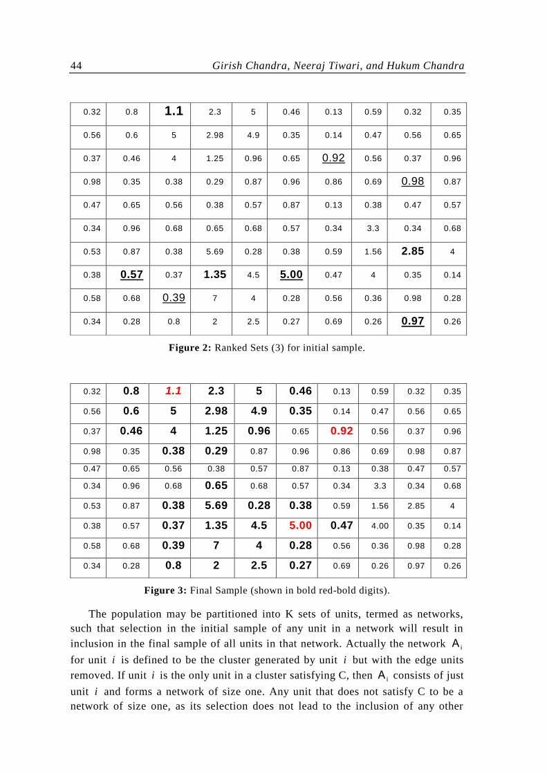
44 Girish Chandra, Neeraj Tiwari, and Hukum Chandra
Figure 2: Ranked Sets (3) for initial sample.
Figure 3: Final Sample (shown in bold red-bold digits).
The population may be partitioned into K sets of units, termed as networks,
such that selection in the initial sample of any unit in a network will result in
inclusion in the final sample of all units in that network. Actually the network iA
for unit i is defined to be the cluster generated by unit i but with the edge units
removed. If unit i is the only unit in a cluster satisfying C, then iA consists of just
unit i and forms a network of size one. Any unit that does not satisfy C to be a
network of size one, as its selection does not lead to the inclusion of any other
0.32 0.8 1.1 2.3 5 0.46 0.13 0.59 0.32 0.35
0.56 0.6 5 2.98 4.9 0.35 0.14 0.47 0.56 0.65
0.37 0.46 4 1.25 0.96 0.65 0.92 0.56 0.37 0.96
0.98 0.35 0.38 0.29 0.87 0.96 0.86 0.69 0.98 0.87
0.47 0.65 0.56 0.38 0.57 0.87 0.13 0.38 0.47 0.57
0.34 0.96 0.68 0.65 0.68 0.57 0.34 3.3 0.34 0.68
0.53 0.87 0.38 5.69 0.28 0.38 0.59 1.56 2.85 4
0.38 0.57 0.37 1.35 4.5 5.00 0.47 4 0.35 0.14
0.58 0.68 0.39 7 4 0.28 0.56 0.36 0.98 0.28
0.34 0.28 0.8 2 2.5 0.27 0.69 0.26 0.97 0.26
0.32 0.8 1.1 2.3 5 0.46 0.13 0.59 0.32 0.35
0.56 0.6 5 2.98 4.9 0.35 0.14 0.47 0.56 0.65
0.37 0.46 4 1.25 0.96 0.65 0.92 0.56 0.37 0.96
0.98 0.35 0.38 0.29 0.87 0.96 0.86 0.69 0.98 0.87
0.47 0.65 0.56 0.38 0.57 0.87 0.13 0.38 0.47 0.57
0.34 0.96 0.68 0.65 0.68 0.57 0.34 3.3 0.34 0.68
0.53 0.87 0.38 5.69 0.28 0.38 0.59 1.56 2.85 4
0.38 0.57 0.37 1.35 4.5 5.00 0.47 4.00 0.35 0.14
0.58 0.68 0.39 7 4 0.28 0.56 0.36 0.98 0.28
0.34 0.28 0.8 2 2.5 0.27 0.69 0.26 0.97 0.26

Adaptive Cluster Sampling Based on Ranked Sets 45
units. This means that all clusters of size one are also networks of size one. Here
we should note that any cluster consisting of more than one unit can be split into a
network and further networks of size one, as each edge units are the networks of
size one. It is also clear that all the K networks are disjoint.
Let the final reduced sample is denoted by the unordered set 21, sss , where
1s is the set of n unordered labels from the initial sample (which are distinct, as
sampling is without replacement in the first phase), and 2s is the set of distinct
unordered labels from the remainder of the sample s. The sampling design is a
function ysp assigning a probability to every possible sample s. In designs such
as those described in this paper, these selection probabilities depend on the
population y-values. Let im denote the number of units in iA , and let ia , denote
the total number of units in networks of which unit i is an edge unit. If unit i
satisfy C, then ia =0, while if unit i does not satisfies C, then 1im . The
probability that the unit i is included in the sample 1s is given by,
N
amp ii i
The probability that unit i is included in the sample s is
n
N
n
amN ii
i 1
.
(2.1)
3 Estimators of the population mean
Generally with the adaptive cluster sampling designs, standard est imators of the
population mean and total are not unbiased. However, the classical estimators such
as the sample mean Y based on simple random sampling and Y based on the
clusters with selection probabilities proportional to cluster size are unbiased under
the non-adaptive designs. In this Section some estimators are given that are
unbiased with the adaptive cluster sampling design discussed in this paper. These
unbiased estimators do not depend on any assumptions about the population.
Let S denote the set of all possible samples. The expected value of an
estimator t is defined in the design sense and is defined as,
Ss
s spt)t(E y , (3.1)

46 Girish Chandra, Neeraj Tiwari, and Hukum Chandra
where st is the value of the estimate for the sample s.
3.1 The initial sample mean
If the final sample of the proposed design is selected in the first phase only, the
estimator of population mean µ is unbiased as ranked set sample mean is always
unbiased estimator of µ for finite population. This estimator ignores all units
adaptively added to the sample.
Let ):( niy is the measured y-value of the thi smallest unit in the thi set, an
unbiased estimator of µ based on the initial sample is
n
i
niyn
t1
):(1
1 . (3.2)
As each ):( niy is independent and identical with mean ni: (say), the variance
of 1t is given by
n
i
n
i
ni
nininn
yEn
tVar1
2
2
1
:22
::21
1
, (3.3)
where 2 is the population variance. Generally ni: , ni .....,2,1 are unknown and
can be estimated by the average of the thi smallest ranked unit of each set.
3.2 An estimator based on initial intersection probabilities
If we know the inclusion probability i that unit i is included in the sample s for
all the sampled units, we can use the Horvitz-Thompson estimator, given by
si
N
i i
ii
i
i
HT
Iy
N
y
N 1
11ˆ
, (3.4)
where iI is the indicator variable which takes the value 1 when unit i is included
in the sample and 0 otherwise. Unfortunately, although im is known in (2.1) for all
the units in s, but some of the ia ‟s are unknown. For example, if unit i is an edge
unit for some clusters in the sample, then all the clusters in which it belongs to,
would not generally be sampled, so that ia will be unknown for those clusters. To

Adaptive Cluster Sampling Based on Ranked Sets 47
get around this problem Thompson (1990) dropped ia from i and considered the
partial inclusion probability
n
N
n
mN i
i 1/ . (3.5)
Thus observations that do not satisfy the condition C are ignored if they are
not included in 1s . He used the sample of n networks (some of which may be
same), rather than the n clusters, for estimating µ. The probability /
i can then be
interpreted as the probability that the initial sample 1s intersects iA , the network
for unit i.
The unbiased estimator 2t based on the initial intersection probabilities takes
the form
N
i i
ii Iy
Nt
1/
/
2
1
, (3.6)
where /
iI takes the value 1 (which probability /
i ) if 1s intersects iA , and 0
otherwise.
It is more convenient to write the summation part of the estimator 2t in (3.6)
in terms of the distinct networks, as the intersection probability /
i is same (= k ,
say) for each unit i in the thk network. Hence
/
1
*
1
*
2
11 K
k k
kK
k k
kk y
N
Jy
Nt
, (3.7)
where *
ky is the sum of the y-values for the network k, K is the total number of
distinct networks in the population, /K is the number of distinct networks in the
sample s, and kJ takes a value of 1 (with probability k ) if the initial sample
intersects the network k, and 0 otherwise. If there are kx units in the network k,
then

48 Girish Chandra, Neeraj Tiwari, and Hukum Chandra
n
N
n
xN k
k 1 (3.8)
Also letting jkp =P ( thj and thk network not intersected), then
11 kjjk JJPp
n
N
n
xxN kj
. (3.9)
Therefore the probability that the networks j and k are both intersected is
11 kjjk JJP
1111 kjkj JJPJPJP
jkkj p 1
or
n
N
n
xxN
n
xN
n
xN kjkj
jk 1 . (3.10)
With the convention that jjj , the variance of 2t is
K
j
K
k kj
kjjk
kj yyN
tVar1 1
**
22
1
. (3.11)
An unbiased estimator of the variance of 2t is
K
j
K
k
kj
kjjk
kjjk
kj JJyyN
tVar1 1
**
22
^ 1
/ /K
1j
K
1k kjjk
kjjk*
k
*
j2yy
N
1
, (3.12)
provided that none of the joint probabilities jk is zero.
Just as the Horvitz-Thompson estimator has small variance when the y-values
are approximately proportional to the inclusion probabilities, the estimator 2t

Adaptive Cluster Sampling Based on Ranked Sets 49
should have low variance when the network totals *
ky ‟s are proportional to the
intersection probability k .
3.3 Improvement of the estimators using the Rao-Blackwell
method
The estimators 1t and 2t of µ are although unbiased but are not the function of the
minimal sufficient statistic, and so each may be improved by the Rao-Blackwell
theorem by taking conditional expectation, given the minimal sufficient statistic.
For finite population Basu (1969) suggested that the minimal sufficient statistic D
is the unordered set of distinct, labelled observations, that is,
skykD k :, .
Starting with any one of the unbiased estimators DtEtRB . Let /n denote
the number of distinct units in the final adaptive sample s. If the initial sample 1s
is selected without replacement, define
n
nG
/
, the number of possible
combinations of n distinct units from the /n in the sample. Suppose that these
combinations are indexed in an arbitrary way by the label g (g = 1, 2 ….G). Let gt
denote the value of t when 1s consists of combination g and let tVarg
^
denote the
value of the unbiased estimator tVar^
, when computed using the thg combination.
An initial sample that gives rise through the design to the given value D of the
minimal sufficient statistic is called compatible with D. Let the thg indicator
variable ( gI ) takes the value 1 if the thg combination could give rise to D (i.e., is
compatible with D), and 0 otherwise. The number of compatible combinations is
then
G
g
gI1
. (3.13)
Now the estimator t may be improved using Rao-Blackwell theorem and is the
average of the values of t obtained over all those initial samples that are
compatible with D. This improved estimator RBt is
1
1
g
gRB tDtEt
or

50 Girish Chandra, Neeraj Tiwari, and Hukum Chandra
g
G
g
gRB Itt
1
1
(3.14)
and its variance is given by
DtVarEtVartVar RB . (3.15)
An unbiased estimator of the variance of RBt due to Thompson (1990) is given by
g
G
g
RBggRB ItttVartVar
1
2^^ 1
. (3.16)
4 Example
To demonstrate the utility of the proposed procedure and its superiority over the
existing procedures, we use a small artificial population of five units with y-values
/4,15,3,500,2y . The neighbourhood of each unit includes its immediately
adjacent units (of which there are either one or two units). The condition C is
defined by C= 5: yy and the initial sample size n=2.
With the proposed design in which the initial sample is selected by ranked set
sampling, there are 302
3
2
5
possible combinations of units; each combination
has two sets, each of size 2. All 30 possible initial samples from these
combinations are given in the first column of Table 1. The final sample is given in
the second column of the Table 1. In this population the 1st
, 2nd
and 3rd
units, with
y-values 2, 500, and 3, form a cluster consisting of 3 networks each of size 1.
In the first row of the Table 1, the 1st
and 2nd
units of the population, with y-
values 2 and 500, are selected initially. Since 5500 , the single neighbour of the
2nd
unit, having y-value 3, is then added to the sample. The other neighbours of 2nd
unit, having y-value 2 is selected as a member of initial sample, hence is not
selected again. Ignoring the edge units, the results for the estimators of first
sample (i.e. of the first row of Table 1) are given below:
The initial sample mean 251t1 .
The values 1 and 2 are 4.01 and 7.02 , leading to 2t 251.
The classical estimators are 3.168y and 3.168y .
The values of the Rao-Blackwell version of any of the estimators for each
sample are obtained by averaging the value of the corresponding estimator over
those samples that are compatible with D. For the first sample of this example
25.251t RB1 and 25.251t RB2 .

Adaptive Cluster Sampling Based on Ranked Sets 51
Table 1: Observations under the proposed procedure.
The population mean is 104.8, and the population variance is 48834.7. From
Table 1, it is clear that the estimators 1t , 2t , RBt1 and RBt2 are unbiased, whereas
the estimators y and y , used with adaptive design are biased.
S.No 1s 2s 1t 2t RBt1 RBt2 y y
1 (2, 500) (2, 500,3) 251.0 251.0 251.3 251.3 168.3 168.3
2 (2, 15) (2, 15,3,4) 8.5 8.5 8.5 8.5 6.0 4.7
3 (2, 500) (2, 500,3) 251.0 251.0 251.3 251.3 168.3 168.3
4 (2, 500) (2, 500,3) 251.0 251.0 251.3 251.3 168.3 168.3
5 (2, 4) (2, 4) 3.0 3.0 3.0 3.0 3.0 3.0
6 (2, 500) (2, 500,3) 251.0 251.0 251.3 251.3 168.3 168.3
7 (2, 15) (2, 15,3,4) 8.5 8.5 8.5 8.5 6.0 4.7
8 (2, 4) (2, 4) 3.0 3.0 3.0 3.0 3.0 3.0
9 (2, 15) (2, 15,3,4) 8.5 8.5 8.5 8.5 6.0 4.7
10 (2, 15) (2, 15,3,4) 8.5 8.5 8.5 8.5 6.0 4.7
11 (2, 500) (2, 500,3) 251.0 251.0 251.3 251.3 168.3 168.3
12 (2, 500) (2, 500,3) 251.0 251.0 251.3 251.3 168.3 168.3
13 (3, 500) (3, 500,2) 251.5 251.5 251.3 251.3 168.3 168.3
14 (3, 15) (3, 15,4) 9.0 9.0 9.3 9.3 22.0 7.3
15 (3, 500) (3, 500,2) 251.5 251.5 251.3 251.3 168.3 168.3
16 (15, 3) (15, 3,4) 9.0 9.0 9.3 9.3 22.0 7.3
17 (4, 3) (4, 3) 3.5 3.5 3.5 3.5 3.5 3.5
18 (4, 3) (4, 3) 3.5 3.5 3.5 3.5 3.5 3.5
19 (3, 15) (3, 15,4) 9.0 9.0 9.3 9.3 22.0 7.3
20 (3, 15) (3, 15,4) 9.0 9.0 9.3 9.3 22.0 7.3
21 (4, 15) (4, 15,3) 9.5 9.5 9.3 9.3 168.3 7.3
22 (3, 500) (3, 500,2) 251.5 251.5 251.3 251.3 168.3 168.3
23 (3, 500) (3, 500,2) 251.5 251.5 251.3 251.3 168.3 168.3
24 (4, 500) (4, 500,2,3) 252.0 252.0 252.0 252.0 127.3 86.2
25 (3, 4) (3, 4) 3.5 3.5 3.5 3.5 3.5 3.5
26 (3, 4) (3, 4) 3.5 3.5 3.5 3.5 3.5 3.5
27 (15, 4) (15, 4,3) 9.5 9.5 9.3 9.3 168.3 7.3
28 (4, 15) (4, 15,3) 9.5 9.5 9.3 9.3 168.3 7.3
29 (4, 500) (4, 500,2,3) 252.0 252.0 252.0 252.0 127.3 86.2
30 (15, 4) (15, 4,3) 9.5 9.5 9.3 9.3 168.3 7.3
MEAN 104.8 104.8 104.8 104.8 91.4 65.1
BIAS 0.0 0.0 0.0 0.0 -13.4 -39.7

52 Girish Chandra, Neeraj Tiwari, and Hukum Chandra
With the adaptive design in which the initial sample is selected by SRS
without replacement, there are 102
5
possible samples, each having probability
1/10. The final sample and the values of each estimator with mean and variance
are listed in Table 2.
Table 2: Observations under Thompson‟s adaptive design.
From Table 1 and Table 2, it may be concluded that for this small artificial
example, the proposed procedure gives more average yield for almost all the
estimators in comparison to that given by the procedure of Thompson (1990).
5 Conclusion
When the measurements of units are very costly and time consuming and there is
heterogeneity between the units of the population, the simple random sampling
become useless. In such situations, RSS is a cost-effective and precise method of
sample selection. In this discussion, we have used the technique of RSS to select
the initial sample under adaptive sampling. The proposed design is more efficient
than adaptive cluster sampling based on simple random sampling for estimating
rare and endangered population, under the assumption that ranking of sampling
units are easier than actual measurements. It also contains the information about
all order statistics. Relative precision of RSS compared with SRS is an increasing
function of set size (k). It shows that the efficiency of proposed design increases as
k in the first phase of the design increases. We have demonstrated theoretically as
well as with the help of an artificial example that the proposed procedure is more
advantageous in comparison to existing procedures of adaptive sampling in the
S.No. 2s 1t 2t RBt1 RBt2 y
1 (2, 500,3) 251.00 143.86 251.25 144.11 168.33
2 (2, 3) 2.50 2.50 127.00 73.43 2.5
3 (2, 15, 4) 8.50 5.29 4.25 2.64 7
4 (2, 4) 3.00 3.00 127.50 73.93 3
5 (500, 3, 2) 251.50 144.36 251.25 144.11 168.33
6 (500, 15, 2, 3, 4) 257.50 147.14 257.50 147.14 104.8
7 (500,4, 2) 252.00 144.86 254.75 146.00 168.67
8 (3, 15, 4) 9.00 5.79 8.75 6.04 7.33
9 (3,4) 3.50 3.50 7.00 5.19 3.5
10 (15, 4, 3) 8.50 6.29 8.75 6.04 7.33
MEAN 104.70 60.66 129.80 74.86 64.08

Adaptive Cluster Sampling Based on Ranked Sets 53
sense that it provides unbiased estimators as well as it give equal importance to all
the rank orders and as such it is more informative. The proposed design also
establishes a bridge between the ranked set sampling and adaptive cluster
sampling and uses the advantage of both the schemes. However, data availability
in the form of ranked clusters has to be determined in advance. As there are only
few sampling procedures in the area of rare species estimation as well as when the
measurement of units are difficult and costly in comparison to the ranking of units
by inexpensive techniques including visual inspection, the doors are open in future
to develop the strategy for extracting the benefits of the two schemes. The
proposed procedure has also particular relevance to assess the effects of human
induced activities in the flora, fauna etc., that increase species rarity.
Acknowledgement
The authors are grateful to the Editor and an anonymous referee for their
constructive comments and suggestions, which led to considerable improvement in
presentation of this manuscript. We are also thankful to Ministry of Statistics and
Program Implementation, Government of India for providing the fund to present
the paper in the International Conference on Applied Statstics-2010 at
Ribno, Slovenia.
References
[1] Barnett, V. and Moore, K. (1997): Best linear unbiased estimates in ranked
set sampling with particular reference to imperfect ordering. Journal of
Applied Statistics, 24, 697-710.
[2] Basu, D. (1969): Role of the sufficiency and likelihood principle in sample
survey theory. Sankhya, 31(A), 441-454.
[3] Blanke, D. (2006): Adaptive sampling schemes for density estimation.
Journal of Statistical Planning and Inference, 136, 2898-2917.
[4] Chaudhuri, A., Bose, M., and Ghosh, J.K. (2004): An application of adaptive
sampling to estimate highly localized population segments. Journal of
Statistical Planning and Inference, 121, 175-189.
[5] Chen, Z., Bai, Z.D., and Sinha, B.K. (2004): Ranked Set Sampling: Theory
and Applications. New York: Springer-Verlag.
[6] Cobby, J.M., Ridout, M.S., Bassett, P.J., and Large, R.V. (1985): An
investigation into the use of ranked set sampling on grass and grass-clover
swards. Grass and Forage Science, 40, 257-263.
[7] Halls, L.K. and Dell, T.R. (1966): Trials of ranked set sampling for forage
yields. Forest Science, 12, 22-26.

54 Girish Chandra, Neeraj Tiwari, and Hukum Chandra
[8] Hu, J. and Su, Z. (2007): Adaptive resampling algorithms for estimating
bootstrap distributions. Journal of Statistical Planning and Inference, article
in press.
[9] Kaur, A., Patil, G.P., Sinha, A.K., and Taillie, C. (1995): Ranked set
sampling, an annotated bibliography. Environmental and Ecological
Statistics, 2, 25-54.
[10] Martin, W.L., Sharik, T.L., Oderwald, R.G., and Smith, D.W. (1980):
Evaluation of Ranked Set Sampling for Estimating Shrub Phytomass in
Appalachian Oak Forests. Blacksburg, Virginia: School of Forestry and
Wildlife Resources, Virginia Polytechnic Institute and State University, FWS,
4-80.
[11] McIntyre, G.A. (1952): A method for unbiased selective sampling using
ranked sets. Australian Journal of Agricultural Research, 3, 385-390.
[12] McIntyre, G.A. (1978): Statistical aspects of vegetation sampling. In
Mannetje, L.T. (Ed.): Measurement of Grassland Vegetation and Animal
Production Bulletin, 52, Hurley, Berkshire: Commonwealth Bureau of
Pastures and Field Crops. 8-21.
[13] Muttlak, H.A. and McDonald, L.L. (1992): Ranked set sampling and the line
intercept method: A more efficient procedure. Biometrical Journal, 34, 329-
346.
[14] Nahhas, R.W., Wolfe, D.A., and Chen, H. (2002): Ranked set sampling: Cost
and optimal set size. Biometrics, 58, 964-971.
[15] Patil, G.P., Sinha, A.K., and Taillie, C. (1994): Ranked set sampling. In Patil,
G.P. and Rao, C.R. (Eds.): Handbook of Statistics, New York: Elsevier
Science Publishers, 167-199.
[16] Roesch, F.A., Jr. (1993): Adaptive cluster sampling for forest inventories.
Forest Science, 39, 655-669.
[17] Salehi, M.M. and Seber, G.A.F. (1997): Two stage adaptive cluster sampling.
Biometrics, 53, 959-970.
[18] Salehi, M.M. and Seber, G.A.F. (2004): A general inverse sampling scheme
and its application to adaptive cluster sampling. Australian and New Zealand
Journal of Statistics, 46, 483-494.
[19] Stokes, S.L. and Sager, T.W. (1988): Characterization of a ranked set sample
with application to estimating distribution functions. Journal of the American
Statistical Association, 83, 374-381.
[20] Thompson, S.K. (1990): Adaptive cluster sampling. Journal of the American
Statistical Association, 85, 1050-1059.
[21] Thompson, S.K. (1991a): Stratified adaptive cluster sampling. Biometrika,
78, 389-397.
[22] Thompson, S.K. (1991b): Adaptive cluster sampling: Designs with primary
and secondary units. Biometrics, 47, 1103-1115.

Adaptive Cluster Sampling Based on Ranked Sets 55
[23] Thompson, S.K. (1996): Adaptive cluster sampling based on order statistics.
Environmetrics, 7, 123-133.
[24] Thompson, S.K. and Seber, G.A.F. (1996): Adaptive Sampling, New York:
Wiley.
![MIXED DOUBLE-RANKED SET SAMPLING: A MORE ...Ranked set sampling (RSS), a data collection scheme, was rst implemented by [9] as a good competitor to simple random sampling (SRS) scheme](https://img.dokumen.tips/doc/110x75/5f9d1c71e02ac73fbe49eca5/mixed-double-ranked-set-sampling-a-more-ranked-set-sampling-rss-a-data-collection.jpg)