Adaptation and diversity along an altitudinal gradient in

Tanto Hadado et al. BMC Plant Biology 2010, 10:121http://www.biomedcentral.com/1471-2229/10/121

Open AccessR E S E A R C H A R T I C L E

Research articleAdaptation and diversity along an altitudinal gradient in Ethiopian barley (Hordeum vulgare L.) landraces revealed by molecular analysisTesema Tanto Hadado1,2, Domenico Rau1,3, Elena Bitocchi1 and Roberto Papa*1

AbstractBackground: Among the cereal crops, barley is the species with the greatest adaptability to a wide range of environments. To determine the level and structure of genetic diversity in barley (Hordeum vulgare L.) landraces from the central highlands of Ethiopia, we have examined the molecular variation at seven nuclear microsatellite loci.

Results: A total of 106 landrace populations were sampled in the two growing seasons (Meher and Belg; the long and short rainy seasons, respectively), across three districts (Ankober, Mojanawadera and Tarmaber), and within each district along an altitudinal gradient (from 1,798 to 3,324 m a.s.l). Overall, although significant, the divergence (e.g. FST) is very low between seasons and geographical districts, while it is high between different classes of altitude. Selection for adaptation to different altitudes appears to be the main factor that has determined the observed clinal variation, along with population-size effects.

Conclusions: Our data show that barley landraces from Ethiopia are constituted by highly variable local populations (farmer's fields) that have large within-population diversity. These landraces are also shown to be locally adapted, with the major driving force that has shaped their population structure being consistent with selection for adaptation along an altitudinal gradient. Overall, our study highlights the potential of such landraces as a source of useful alleles. Furthermore, these landraces also represent an ideal system to study the processes of adaptation and for the identification of genes and genomic regions that have adaptive roles in crop species.

BackgroundAmong the cereal crops, barley is the species that pres-ents the highest adaptability to a wide range of environ-ments. It is cultivated from arctic latitudes to tropicalareas, and it is grown at the highest altitudes. In Tibet,Nepal, Ethiopia and the Andes, farmers cultivate barleyon mountain slopes at altitudes higher than any othercereals [1,2].

Ethiopia is probably the region of barley cultivation thatpresents the highest variability for climatic and edaphicconditions. It is cultivated from 1,400 m above sea level(a.s.l.) to over 4,000 m a.s.l., and it has adapted to specificsets of agro-ecological and microclimatic regimesthroughout the country [3]. Landraces represent over90% of the barley cultivated in Ethiopia. In contrast to the

genetic uniformity of modern cultivars, landraces showvariation both between and within populations. Thiswithin-population diversity of these barley landracesmight allow them to cope with environmental stresses,which is very important for achieving yield stability [4].For this reason, landraces represent a very interestingmodel to study the processes of adaptation and for identi-fication of genes and genomic regions that have adaptiveroles in a crop species, through association mapping [5-8]and through scanning for signatures of selection at themolecular level [9-13].

Knowledge of the population structure of Ethiopianbarley landraces, together with a deeper understanding ofthe nature and extent of their variation, is an importantprerequisite for efficient conservation and use of theexisting plant materials. Several studies have reported ahigh level of genetic diversity in barley populations fromEthiopia, such as those based on morphological traits[14-16], and on biochemical data [17,18]. Moreover, Ethi-

* Correspondence: [email protected] Dipartimento di Scienze Ambientali e delle Produzioni Vegetali, Università Politecnica delle Marche, Via Brecce Bianche, 60131 Ancona, ItalyFull list of author information is available at the end of the article

© 2010 Hadado et al; licensee BioMed Central Ltd. This is an Open Access article distributed under the terms of the Creative CommonsAttribution License (http://creativecommons.org/licenses/by/2.0), which permits unrestricted use, distribution, and reproduction inany medium, provided the original work is properly cited.

http://www.ncbi.nlm.nih.gov/entrez/query.fcgi?cmd=Retrieve&db=PubMed&dopt=Abstract&list_uids=20565982


Page 2 of 20

opian barley is a precious source of genes that controlimportant agronomic traits, such as resistance to disease(e.g. powdery mildew, barley yellow dwarf virus, netblotch, scald and loose smut) and to insect attack [19-25],high lysine, and protein quality and content [26], andmalting and brewing quality [27]. Furthermore, the greatvariability of environmental conditions in Ethiopia thatpromote adaptive divergence, and the cultivation of bar-ley in two growing seasons per year [16], have probablydriven the structure of variation of these landraces.

Numerous studies on Ethiopian barley have detectedcorrelations between altitude and the frequency of mor-phological [14-16,28], agronomic [24,29] and biochemi-cal [30] traits, including pathogen resistance[20,24,25,29]. Altitudinal gradients provide substantialchanges in numerous environmental variables, which alsoinclude atmospheric pressure, temperature, clear-sky tur-bidity, UV-B radiation, and humidity. Furthermore, thecombined environmental changes across altitudes caninfluence various biological processes in plants, and canthus result in adaptive changes and constraints on thegenetic diversity of plant populations. Associationbetween environmental variables and allele frequenciescan be maintained by a balance between selection andgene flow [31-33]. However, in contrast to latitudinalclines, altitudinal gradients involve dramatic ecologicaltransitions over relatively short linear distances, and sothey require especially strong selection to counterbalancethe homogenising effects of gene flow [34]. Nevertheless,the interactions between drift and spatially restrictedgene flow or historical patterns of colonisation (admix-ture between previously isolated populations) might alsoexplain clinal variation.

The present study is based on a large collection of Ethi-opian barley landraces (3,170 individual plants, for a totalof 106 landrace populations) that was established in 2005in the North Shewa zone (Amhara region, Ethiopia), fromfarmers who have used their own seed for generations[16]. The collection was obtained through visiting thesame three districts (Ankober, Mojanawadera and Tarm-aber) in both the Meher and Belg growing seasons [16](see [16], for further details). Here, we have analysed themolecular diversity and genetic structure of this collec-tion, using simple sequence repeats (SSRs), while takinginto account not only the environmental adaptation (geo-graphical and altitude factors), but also, for the first time,the two growing seasons per year.

ResultsLevel of polymorphismSeven mapped nuclear SSRs were used to examine thelevels and patterns of genetic variation of the barley lan-draces collected in North Shewa, in the central highlandsof Ethiopia [16]. Table 1 provides a summary of the statis-

tics computed considering each of the two seasons (Belgand Meher), the three districts (Ankober, Mojanawadera,and Tarmaber) and the three altitude classes (<2,300,2,300-2,800, >2,800 m a.s.l.). The same statistics were alsocomputed for each locus, and are given in Additional file1. A total of 66 alleles were detected, with the number ofalleles per locus (na) ranging from four (HVM20 andHVM67) to 23 (Bmac0156), with an average of 9.4 allelesper locus.

The variation between seasons was not significantacross any of the statistics considered (Wilcoxon signed-paired rank test), while the only significant differenceamong the districts (Wilcoxon signed-paired rank test,after Bonferroni correction, P = 0.03) was for the allelicrichness between the Ankober (RS = 8.22) and Tarmaberdistricts (RS = 7.11; Table 1). For the altitude classes,more marked differences were seen (Table 1). The num-ber of alleles (na) and the allelic richness (RS) of the lowaltitude class (<2,300 m a.s.l.: na = 39 and RS = 5.57) werelower than those of the intermediate altitude class (2,300-2,800 m a.s.l.: na = 50 and RS = 7.10; difference margin-ally non-significant, P = 0.06, Wilcoxon signed-pairedrank test, after Bonferroni correction) and of the highaltitude class (>2800 m a.s.l.: na = 57, P = 0.06, and RS =7.40, P = 0.09). The genetic diversity (He) of the interme-diate altitude class (He = 0.65) was significantly higher(Wilcoxon signed-paired rank test, after Bonferroni cor-rection, P = 0.03) than that of the high altitude class (He =0.57).

Considering the pattern of private alleles, the two sea-sons did not share 14 (21%) out of the 66 SSR alleles, witheach of these showing a frequency lower than 5%. Thethree districts showed a total of 15 private alleles (23%),three of which had a frequency higher than 5%. Finally,compared to seasons and districts, the altitude classeshad a higher number of private alleles (17; 26%), four ofwhich (one for <2,300 m a.s.l., and three for >2,800 ma.s.l.) had a frequency higher than 5%. Moreover, theaverage frequency of private alleles that showed a fre-quency higher than 5% was 0.00 for seasons, 0.063 for dis-tricts, and 0.085 for altitude classes.

The overall level of observed heterozygosity was verylow (0.003). Only three individuals, all located at highaltitude, showed one or two heterozygous loci. Overall,the average genetic diversity (He, [35]) in the Ethiopianbarley landraces was 83.5% of the diversity found in theSyrian and Jordanian barley landraces (Table 2). This dif-ference was significant (Wilcoxon signed-paired ranktest, P = 0.05). A significant gap (-31.2%) was also seen forthe number of alleles, na (Wilcoxon signed-paired ranktest, P = 0.01).

Although it is important to consider the differences inthe sample sizes, the Ethiopian barley landraces showed a

Tant

o H

adad

o et

al.

BMC

Plan

t Bio

logy

201

0, 1

0:12

1ht

tp://

ww

w.b

iom

edce

ntra

l.com

/147

1-22

29/1

0/12

1Pa

ge 3

of 2

0

Table 1: Summary statistics for the seasons, districts and altitude classes, and for the whole sample.

S na no ne He Ho RS Number of private alleles

Average frequency of private alleles

Number of private alleles (freq. ≥ 0.05)

Average frequency of private alleles (freq. ≥ 0.05)

Seasons

Belg 108 60 8.57 4.71 0.63 0.001 8.57 8 0.01 0 -

Meher 104 58 8.29 4.54 0.67 0.004 8.28 6 0.02 0 -

Districts

Ankober 72 58 8.29 4.86 0.66 0.006 8.22 9 0.03 2 0.07

Mojanawadera 64 53 7.57 4.67 0.63 0.002 7.57 4 0.03 1 0.05

Tarmaber 76 50 7.14 3.86 0.64 0.000 7.11 2 0.02 0 -

Altitude classes (m a.s.l.)

<2,300 46 39 5.57 3.11 0.65 0.000 5.57 2 0.04 1 0.07

2,300-2,800 54 50 7.14 4.45 0.66 0.000 7.10 3 0.02 0 -

>2,800 112 57 8.14 4.24 0.57 0.009 7.40 12 0.03 3 0.09

ALL 212 66 9.43 4.96 0.66 0.003 9.43 - - - -

S, sample size; na, number of observed alleles; no, average number of observed alleles per locus; ne, effective number of alleles per locus; He, unbiased expected heterozygosity; Ho, observed heterozygosity; RS, allelic richness.


Page 4 of 20

higher number of alleles (na = 62, not considering theHVM20 locus) than seen for both the Nepalese barleylandraces (na = 44) [36] and the modern varieties (na = 41)[37] (Table 2).

The divergence (FST and RST) estimates between theseasons, districts, and altitude classes are given in Table 3.The genetic differentiation between the two seasons waslow for both FST (0.02) and RST (0.01), even if in contrastto RST, the FST was significantly different from zero (P <0.001). A slightly higher level of differentiation was seenfor districts (FST = 0.02, P < 0.01; RST = 0.03, P < 0.05).Among the altitude classes, the levels of differentiationwere higher compared to seasons and districts, both forFST (0.10, P < 0.001) and RST (0.09, P < 0.001). The diver-gence (FST and RST) estimates between seasons, districtsand altitude classes for each of the SSR loci analysed are

given in Additional file 2. The individual SSR loci diver-gence (FST,) between seasons was significant for four loci(Bmag0013, HVM67, Bmac0040, and Bmac0134), even ifthe values were low, and varied from 0.02 to 0.05 (Addi-tional file 2). The Bmag0013 locus was the only one forwhich the divergence was higher between seasons (FST =0.05) than among districts or altitude classes (FST = 0.01and 0.03 respectively; Additional file 2). A similar trendwas seen for districts, with three low significance valuesranking from 0.02 (Bmac0156) to 0.04 (Bmac0134). Forthe altitude classes, the situation was different; indeed, allof the SSR loci were significantly differentiated amongthe altitude classes, with values varying from 0.03(Bmag0013) to 0.28 (HVM67).

Table 4 reports the divergence estimates (FST) amongthe three districts within the same altitude classes (<2,300m a.s.l.; 2,300-2,800 m a.s.l., and >2,800 m a.s.l.). The dif-ferentiation among the low altitude classes of the threedistricts was higher (FST = 0.10, P < 0.01) than thatamong the three districts within the intermediate (FST =0.04, P > 0.05) and high (FST = 0.01, P > 0.05) altitudeclasses.

Population structure and altitude cline of genetic variationRecently, various studies (mainly in the field of humangenetics [38,39]) have questioned the reliability of theSTRUCTURE results in cases of complex genetic struc-tures. In particular, this debate has considered whether

Table 2: Diversity of landraces from Ethiopia compared with those from Syria, Jordan and Nepal, and with modern varieties.

SSR locus name

HVM20 (ch1H)

Bmac0134 (ch2H)

Bmag0013 (ch3H)

HVM67 (4H)

Bmac0113 (ch5H)

Bmac0040 (ch6H)

Bmac0156 (ch7H)

Total na

Mean H

na H na H na H na H na H na H na H

Ethiopian landraces (209)

4 0.32 11 0.80 6 0.81 4 0.41 7 0.47 11 0.86 23 0.93 66 (62)1 0.66 (0.71)1

Syrian and Jordanian

landraces (125)2

5 0.56 17 0.90 11 0.80 5 0.65 9 0.80 18 0.88 31 0.91 96 (91)1 0.79 (0.82)1

Nepalese landraces (107)3

- - 3 0.44 8 0.26 5 0.30 9 0.83 2 0.02 17 0.87 44 0.50

Modern varieties (24)3

- - 7 0.79 6 0.81 3 0.50 6 0.79 12 0.94 9 0.84 41 0.64

1 Total number of alleles and average diversity across loci (in parentheses) are calculated excluding the HVM20 locus, to allow direct comparisons with the Nepalese landraces and with the modern varieties.2 Data from Table 1 of Russel et al. (2003).3 Data from Table 2 of Pandey et al. (2006) for the Nepalese landraces, and from the graphical genotypes represented in Figure 2 of Macaulay et al. (2001) for the modern varieties. In both of these cases, genetic diversity is calculated as polymorphic information content (PIC), following Weber (1990).

Table 3: Divergence (FST and RST) estimates between seasons, districts and altitude classes.

FST RST

Seasons 0.02*** 0.01

Districts 0.02** 0.03*

Altitude classes 0.10*** 0.09***

*P < 0.05; **P < 0.01; ***P < 0.001.


Page 5 of 20

Bayesian clustering algorithms are appropriate tools forstudying genetic structures in populations with continu-ous variation of allele frequencies. To address this prob-lem, the population structure analysis of our collectionwas carried out using two different methods: the first wasthe Pritchard et al. [40] non-spatial Bayesian clusteringmethod implemented in the STRUCTURE software, ver-sion 2.1 [41], and the second was based on a Bayesianclustering algorithm that incorporates spatial informa-tion when identifying clusters of individuals, and wasimplemented in the TESS software, version 2.0 [42].

The plot of the average ln likelihood values over 100runs for K values ranging from 1 to 10 shows that the lnlikelihood estimates increase progressively as K increases.Thus, we used the Evanno et al. [43] method to provide abetter estimate of the 'true' number of clusters (K) thatcharacterised our sample. The highest ΔK value wasfound at K = 2, although high values of ΔK were foundalso for K = 3, 4 and 10. To minimise the effects of outlierruns, we also computed the ΔK value considering five

random re-samplings of 80 of the 100 runs for each Kvalue. In all cases, the highest ΔK corresponded to K = 2.Thus, hereafter, we will refer to cluster S1 and cluster S2for the K = 2 populations identified by STRUCTURE.

The percentages of membership (q), or inferred groupancestries, of the individuals in each of the two clusterswere computed. One hundred and ninety-seven individu-als (93%) had a q higher than 0.70, in 192 individuals(91%), q was higher than 0.80, and in 183 (86%), it washigher than 0.90. Considering the threshold for member-ship of q ≥ 0.70, cluster S1 included 110 individuals, andcluster S2, 87 individuals.

Figure 1 shows the collection site coordinates and theaverage q values for clusters S1 and S2 of each barley lan-drace.

When the individuals were sorted according to altitude,the STRUCTURE analysis revealed a well-defined cline ofvariation; indeed, at low altitudes, cluster S1 was mainlyseen, and this tended to be substituted by cluster S2 athigh altitudes. The relationships between altitude and qfor cluster S2 were assessed using a simple linear regres-sion model. This regression was significant (R2 = 0.42, F =152.5 and P < 0.0001; Figure 2), and it was consistentwithin the Meher (R2 = 0.45, F = 85.0 and P < 0.0001) andthe Belg (R2 = 0.36, F = 59.4 and P < 0.0001) seasons (Fig-ure 3), and within the three districts (P < 0.0001, R2 =0.54, 0.21, and 0.40, F = 83.6, 17.8, and 50.0; for Ankober,Mojanawadera and Tarmaber, respectively) (Figure 4).

The second approach used for the population structureanalysis was the algorithm implemented in the TESS soft-ware that allows for prior spatial information when iden-tifying clusters of individuals. This TESS software allowsthe testing of different values of the spatial dependentparameter (Ψ); this parameter weights the relative impor-tance given to spatial connectivities. We tested three dif-ferent Ψ: 0.0 (no spatial correlation between individuals),and 0.6 and 1.0 (moderate and strong spatial correlationbetween individuals, respectively). For each Ψ value con-sidered, we performed 100 runs for K from 2 to 10. Thenthe DIC values of the 10 runs with the smallest DIC wereaveraged. In plotting the average DIC values versus K(from 2 to 10), we obtained an inflection point at K = 6.This was the same for all of the different interactionparameter (Ψ) values considered. Thus the best modelwas obtained for K = 6 and the lowest DIC value corre-sponded to Ψ = 0.6, indicating a moderate spatial correla-tion between individuals. The average over 10 runs withthe smallest DIC value q was computed. We defined thesix TESS clusters as T1, T2, T3, T4, T5 and T6. One hun-dred and twenty-five individuals (59%) were assigned toone of the six clusters with a q higher than 0.60, with 104(49%) higher than 0.70, and 70 (33%) higher than 0.80.Figure 5 shows the assignment results for all of the indi-viduals when ordered according to altitude. Averaging the

Table 4: Divergence (FST) estimates between the three different districts within the same altitude classes.

<2,300 m a.s.l. classes FST

Ankober - Mojanawadera 0.16**

Ankober - Tarmaber 0.10*

Mojanawadera - Tarmaber 0.19*

Mean FST0.15

Average unweighted FST0.10**

2,300-2,800 m a.s.l. classes

Ankober - Mojanawadera 0.08*

Ankober - Tarmaber 0.05 ns

Mojanawadera - Tarmaber 0.07*

Mean FST0.07

Average unweighted FST0.04 ns

>2,800 m a.s.l. classes

Ankober - Mojanawadera 0.03*

Ankober - Tarmaber 0.03 ns

Mojanawadera - Tarmaber 0.02 ns

Mean FST0.03

Average unweighted FST0.01 ns

ns, not significant*P < 0.05, **P < 0.01


Page 6 of 20

Figure 1 Map of the collection sites. Collection site coordinates and average q values for clusters S1 (green) and S2 (red) of each of the barley lan-draces. Landraces that showed an average q > 0.70 were considered completely assigned to one of the two clusters identified by STRUCTURE.

Mojandawadera

Tarmaber

Ankober

3033 m a.s.l.

~ 3000 m a.s.l.

~ 3132 m a.s.l.

~ 3324 m a.s.l.

2024m a.s.l.

1830 m a.s.l

~ 33 Km

No main road

~ 50 Km

No main road

Lat

itud

e U

TM

(K

m)

1,120

1,110

1,100

1,090

1,080

1,070

1,060

Longitude UTM (Km)

550 560 570 600580 590

2214 m a.s.l.


Page 7 of 20

q for the six TESS clusters for the three altitude classes,we observed that the previous cline of variation alongaltitude identified by the STRUCTURE assignment wasalso maintained for TESS; indeed, at low altitudes, the T1and T2 clusters were mainly present, and these tended to

be substituted by the T5 and T6 clusters at high altitudes(Figure 6). The T3 cluster was mostly present at interme-diate and high altitudes, while T4 was present in all of thealtitude classes (Figure 6). However, the genotype assign-ment for T4 is more scattered at intermediate and high

Figure 2 Linear regression analysis for altitude and membership coefficient (q) for cluster S2 identified by STRUCTURE.

1.2

1.0

0.8

0.6

0.4

0.2

0.0

1500

Mem

bers

hip

coef

fici

ent

(q)

for

Clu

ster

S2

2000 2500 3000 3500

Altitude (m a.s.l.)

y = -1.6 + 0.0008x

Figure 3 Population structure across seasons and altitudes using STRUCTURE. STRUCTURE assignment at K = 2 for the 108 individuals collected during the Belg growing season and the 104 individuals collected during the Meher season, ordered according to crescent altitude levels. Green, clus-ter S1; red, cluster S2.

2024 2324 2855 3166

Altitude (m a.s.l.)

BE

LG

23241798 2855 33242029

Altitude (m a.s.l.)

ME

HE

R

3184


Page 8 of 20

altitudes than at low altitudes (Figure 5). Indeed, at lowaltitudes, this genotype assignment for T4 is characteris-tic of two populations collected during the Meher season.It is important to note that the percentage of individualsthat had a q to one of the six TESS clusters higher than

0.70 is highest (76%) at low altitudes (<2,300 m a.s.l.), anddecreases at intermediate (35%) and high (45%) altitudes.

The correlation analysis using Spearman's rho (ρ) fornon-parametric tests showed that cluster S1 identified bySTRUCTURE was significantly correlated with TESSclusters T1 and T2, and cluster S2 with T5 and T6 (Addi-

Figure 4 Population structure across districts and altitudes using STRUCTURE. STRUCTURE assignment at K = 2 for the individuals collected in the three districts (Ankober, Mojanawadera and Tarmaber), ordered according to crescent altitude levels. Green, cluster S1; red, cluster S2.

1798 2855 3324

Altitude (m a.s.l.)2324

28552324

2214

3033

3133

1974

Altitude (m a.s.l.)

AN

KO

BE

RM

OJA

NA

-W

AD

ER

A

TA

RM

AB

ER

3102

3033

1924

2252

Figure 5 Population structure along the altitude gradient using TESS. TESS assignment at K = 6 for the 212 individuals, ordered according to cres-cent altitude levels. Blue-purple, T1; red, T2; pink, T3; yellow, T4; grey, T5; green, T6.

T1

T2

T3

T4

T5

T6

1798

Altitude (m a.s.l.)2324 2855 3324


Page 9 of 20

tional file 3). The step-wise multiple regression analysisshowed that mainly TESS clusters T1, T2, T3 and T4 pro-vide a better prediction for cluster S1 (R2 = 0.84), and T4,T5 and T6 are the major contributors for cluster S2 (R2 =0.84) (Additional file 4); TESS cluster T4 contributes toboth of the S1 and S2 clusters identified by STRUCTURE.These results are consistent with the relationshipsbetween the altitude and the q for the TESS groups,which was tested by performing a simple regression anal-ysis; indeed this relationship was highly significant (P <0.0001) for the TESS clusters T1, T2, T5 and T6 (R2 =0.25, 0.14, 0.10, 0.22 respectively), significant (P = 0.05)for T3, but not significant for T4 (P = 0.08).

The ANOVA analysis revealed significant correlationsbetween all of the loci considered and the altitude (Addi-tional file 5).

Considering the morphological data, 82% of the charac-ter states considered and studied by Tanto Hadado et al.[16] were significantly correlated with altitude (P < 0.05),79% of which had a probability lower than 0.01; moreover,at least one character state for each of the morphologicaltraits considered was significantly correlated with alti-tude at P < 0.01 (Table 5).

Association between morphological and molecular characterisationsTo investigate the correspondence between the morpho-logical and molecular characterisations, a contingencyanalysis was performed. The genetic groups defined byTESS analysis were considered, and only the genotypesthat were assigned to one of the groups with a q higherthan 0.70 were included in the analysis (104 genotypes inall). No inference was carried out for TESS cluster T3because no genotypes were assigned to this groupaccording to this threshold. The analysis was conductedconsidering the seven morphological traits: kernel-rownumber, spike density, lemma awn barbs, glume colour,lemma type, length of rachilla hair, and lemma colour[16].

The results show that all of the traits except lemma awnbarbs (P = 0.066), were significantly associated with theTESS genetic clusters. The association was higher forlength of rachilla hairs, glume colour and spike density (P< 0.0001), followed by lemma colour (P < 0.001), rownumber (P = 0.003) and lemma type (P = 0.011). The pro-portion of variance of each morphological trait explainedby genetic groups (R2) varied from 36.6% (length ofrachilla hairs) to 13.0% (lemma type), with an average of22.5%. The types and frequencies of each of these sevenqualitative traits in each of the TESS clusters (with theexclusion of T3, as indicated above) are given in Addi-tional file 6.

The relationships between the genetic groups accord-ing to morphological characterisation were assessedusing a non-parametric correlation analysis (Spearman'srho) (Additional file 7). The clusters T1 and T6 (the for-mer mainly present at low altitudes, and the latter at highaltitudes) showed the highest morphological differentia-tion. T1 included mainly six-rowed (65.2%) and irregular(21.7%) types, and was the only group that included two-rowed types (4.4%), and it showed the highest frequencyamong all of the groups for the two-rowed deficient types(8.7%). Both the regular and deficient two-rowed typeswere absent in T6, which included mainly irregular types(74.2%). T1 was characterised by a high frequency ofdense spike types (47.8%), while T6 was characterised bylax types (41.9%), and both of these groups showed highfrequencies of intermediate spike density types (43.5%and 54.9%, respectively). T1 was monomorphic for thelemma awn barbs (rough) and glume colour (white)traits; in contrast, T6 also showed intermediate lemmaawn barb types (12.9%), and brown (35.5%) and black(6.4%) glume colour types. All of the individuals of T6had short rachilla hairs, while those of T1 had both short(52.2%) and long (47.8%) rachilla hair types. Finally, dif-ferences were seen also for the lemma colour trait: T1was mostly represented by white types (82.6%), while T6was mostly represented by black types (74.2%).

Spatial structure and landscape analysisMantel tests between the genetic and geographical dis-tance matrices were significant (r = 0.12, P < 0.001). How-ever, the correlation between molecular and geographicaldistance was about 2-fold lower than that between themolecular distances and differences in altitude (r = 0.28,P < 0.001), and also lower than that between geographyand altitude (r = 0.14, P < 0.001).

The same pattern was seen for the spatial autocorrela-tion analysis, which showed that within a distance class of5 km, positive and significant Moran's I values weredetected. This indicates that the proximal individuals(included those of the same population/field) were moregenetically similar (i.e. related) than expected from a ran-

Figure 6 Average membership coefficient (q) for the six TESS clusters for the three altitude classes. See legend to Figure 5 for colour key.

0.45

0.40

0.35

0.30

0.25

0.20

0.15

0.10

0.05

0.00< 2300 m a.s.l. 2300-2800 m a.s.l. > 2800 m a.s.l.

Mem

bers

hip

coef

fici

ent

(q)


Page 10 of 20

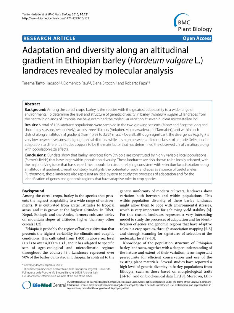
dom distribution (Figure 7a). In this class, the individualsat similar altitudes within each district were compared.The degrees of correlation, however, rapidly decreased,and there were already negative Moran's I values for the10-km distance class. In this class, individuals from rela-tively different altitudes were mostly compared, mainlywithin each district. A similar situation was seen in the20-km and 30-km distance classes. The degrees of corre-lation, however, tended to increase, and interestingly,positive and significant Moran's I values were found forthe 40-km and 50-km distance classes: when individualsof different districts but at similar altitudes (either low orhigh) were compared, they tended to be genetically moresimilar than for a random distribution (Figure 7a). This isparticularly evident considering the relationshipsbetween the genetic and altitude distances; indeed, theindividuals that were collected at similar altitudes showedhigher similarities than those collected at different alti-tudes (Figure 7b).

Finally, it is important to note that based on the distri-bution of the collection sites, when individuals from simi-lar altitudes were compared, they also tended to begeographically more distant. In contrast, the individualsfrom different altitudes were geographically closer (Fig-ure 7c).

Spatial autocorrelation between geographical andgenetic distances was also performed separately for thethree altitude classes (Additional file 8), which confirmedthe previous trends seen, showing at low altitudes (<2,300m a.s.l.) a clear geographical effect (isolation by distancerelationship among plants), while at high altitudes(>2,800 m a.s.l.), this effect disappeared, as all of the simi-larity values were not significantly different from randomvalues, and thus no geographical structure was evident. Anon-significant, intermediate (but as for the >2,800 ma.s.l. class) trend was seen at moderate altitudes (2,300-2,800 m a.s.l).

Table 5: Relationships between frequencies of the character states for each population and altitude (Spearman's rho).

Character Character state1 Spearman's ρ R2 P

Kernel row number Irregular 0.31 0.10 0.001

Six rowed -0.17 0.03 0.09

Spike density Lax 0.02 0.00 0.81

Intermediate 0.37 0.14 0.0001

Dense -0.48 0.23 1.6e-07

Lemma awn barb Intermediate 0.35 0.12 0.0002

Rough -0.34 0.11 0.0004

Glume colour White -0.54 0.29 3.3e-09

Brown 0.62 0.38 2.0e-12

Lemma type No lemma teeth 0.24 0.06 0.01

Lemma teeth -0.24 0.06 0.01

Length of rachilla hair

Short 0.51 0.27 1.6e-08

Long -0.51 0.27 1.6e-08

Kernel colour White -0.53 0.28 6.3e-09

Tan/red 0.39 0.16 2.5e-05

Purple 0.15 0.02 0.13

Black/grey 0.39 0.15 4.2e-05

Morphological data from Tanto Hadado et al. [16].1 Character states with frequencies lower than 0.05 and higher than 0.95 are not included in the analysis.


Page 11 of 20

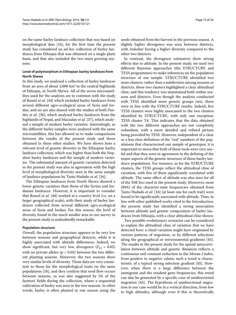
Sliding-window analysisFigure 8 shows the results of the 'sliding-windows' analy-sis. In Figure 8, each point represents: for the y axis, theHe, RS and LD estimates of a group of 40 individuals from20 landrace populations (window); and for the x axis, themean altitude over all of the 20 populations. Thus, thediversity and LD estimates were computed along the alti-tudinal cline. This analysis was carried out separately foreach of the two seasons. The Belg season was not repre-sented at low altitudes, while the Meher season was char-acterised by the whole altitude range considered.

To test the significance of the trends seen, we groupedthe individuals into different and non-overlapping alti-tude ranges: three for Belg: B1, B2 and B3 (average alti-tudes of 2,397, 2,859 and 3,022 m a.s.l., respectively), andfour for Meher: M1, M2, M3, M4 (average altitudes of1,962, 2,416, 2,909 and 3,138 m a.s.l., respectively). Thesignificance was tested between adjacent altitude ranges,using the Wilcoxon signed-paired rank test and the Bon-ferroni correction. The choice of the altitude ranges wasdesigned to have the average altitudes more uniformbetween the Belg (B1, B2, and B3) and the correspondingMeher (M2, M3, M4) classes (the M1 class did not havean equivalent in Belg, which was not represented at lowaltitudes in this analysis). The number of individuals peraltitude range varied from 34 to 40 for Belg, and from 16to 36 for Meher.

Considering the Meher season, the diversity (He)showed a significant increase according to altitude, toabout 2,500 m a.s.l.. Indeed, M2 showed a higher level ofdiversity than M1 (Wilcoxon signed-paired rank test,after Bonferroni correction: P = 0.018); although no othercomparisons were significant in the Meher season, areduction at high altitudes was seen. A significant reduc-tion of He at high altitudes was seen for the Belg season(B2-B3: P = 0.046) (Figure 8a).

The allelic richness, RS, showed a marked increase fromlow to intermediate altitudes in the Meher season (Wil-coxon signed-paired rank test, after Bonferroni correc-tion: M1 < M2: P = 0.017), and reached a plateau atintermediate and high altitudes (M2 vs M3; M3 vs M4)(Figure 8b). For the Belg season, the trend of allelic rich-ness resulted in a slight increase at intermediate altitudes(B1 < B2: P = 0.046) and a decrease at high altitudes (B2 >B3, P = 0.018).

The multilocus LD among our unlinked loci (Figure 8c)decreased with altitude for the season, and interestingly,only that for the Belg season reached non-significant lev-els in the interval between 2,685 and 3,010 m a.s.l. (Figure8c).

DiscussionSeveral studies have analysed the diversity of Ethiopianbarley landraces. However, along with our previous study

Figure 7 Autocorrelation analysis. Results of the autocorrelation analysis using all 212 genotypes and all loci. The 99% probability envelopes are indicated: light blue, upper limit; green, lower limit. Dark blue, observed data: for genetic distance vs geographical distance). Inset: the first 20 km from panel a) (40 classes, 500 m each).

0.08

0.06

0.04

0.02

0.00

- 0.02

- 0.06

0.06

0.04

0.02

0.00

- 0.02

- 0.04

- 0.06

- 0.08

- 0.10

- 0.04

1.4

1.2

1.0

0.8

0.6

Genetic distance vsgeographic distance

Genetic distance vsaltitude

Geographic distancevs altitude

Cit

y-B

lock

D

Mor

anI

Mor

anI

Mor

anI

Geographic distance (Km) Altitude difference (m)Altitude difference (m)

5 10 15 20 25 30 35 40

102 203 305 407 509 610 712 814

102 203 305 407 509 610 712 814

0.06

0.04

0.02

0.00

- 0.02

- 0.04

45

916

916


Page 12 of 20

Figure 8 'Sliding-window' analysis for the two seasons: Belg (blue) and Meher (orange). a) Genetic diversity (He); b) allelic richness (RS); c) mul-tilocus linkage disequilibrium (LD) along the altitudinal cline, with P values also shown. The altitude of each window (20 populations, 40 individuals) was determined by averaging the altitude of the populations (farmers' fields); hence, the differences in the average altitudes between the windows are not constant.

Meher

Unb

iase

dex

pect

edhe

tero

zygo

sity

(He)

0.70

0.65

0.60

0.55

0.50

Belga)

Alle

licR

ichn

ess(R

S) 7.5

7.0

6.5

6.0

5.5

5.0

4.5

b)

P v

alue

Bel

g

2000 2200 2400 2600 2800 3000

0.25

0.15

0.30

0.20

0.10

0.00

0.05Mul

tilo

cus

LD

(r d

)P

val

ue

Meh

er;

Altitude (m a.s.l.)

c)


Page 13 of 20

on the same barley landrace collection that was based onmorphological data [16], for the first time the presentstudy has considered an ad-hoc collection of barley lan-draces from Ethiopia that was obtained on a single-plantbasis, and that also included the two main growing sea-sons.

Level of polymorphism in Ethiopian barley landraces from North ShewaIn this study, we analysed a collection of barley landracesfrom an area of about 2,000 km2 in the central highlandsof Ethiopia, in North Shewa. All of the seven microsatel-lites used for the analyses are in common with the studyof Russel et al. [44] which included barley landraces fromseveral different agro-ecological areas of Syria and Jor-dan, and six are also shared with the studies of both Pan-dey et al. [36], which analysed barley landraces from thehighlands of Nepal, and Macaulay et al. [37], which analy-sed a sample of modern barley varieties. Interestingly, asthe different barley samples were analysed with the samemicrosatellites, this has allowed us to make comparisonsbetween the results of the present study and thoseobtained in these other studies. We have shown here arelevant level of genetic diversity in the Ethiopian barleylandrace collection, which was higher than both the Nep-alese barley landraces and the sample of modern variet-ies. The substantial amount of genetic variation detectedin the present study was also in agreement with the highlevel of morphological diversity seen in the same sampleof landrace populations by Tanto Hadado et al. [16].

The Ethiopian landraces from North Shewa showed alower genetic variation than those of the Syrian and Jor-danian landraces. However, it is important to considerthat Russel et al. [44] worked at a country level (i.e. on alarger geographical scale), with their study of barley lan-draces collected from several different agro-ecologicalareas of Syria and Jordan. For this reason, the level ofdiversity found in the much smaller area in our survey inthe present study is undoubtedly remarkable.

Population structureOverall, the population structure appears to be very lowbetween seasons and geographical districts, while it ishighly associated with altitude differences. Indeed, weshow significant, but very low, divergence (FST = 0.02)with no private alleles (p < 0.05) between the two differ-ent planting seasons. Moreover, the two seasons showvery similar levels of diversity. These data are very consis-tent to those for the morphological traits on the samepopulations [16], and they confirm that seed flow occursbetween seasons, as was also suggested by 5% of thefarmers' fields during the collection, where a sequentialcultivation of barley was seen in the two seasons. In otherwords, barley is often planted in one season using the

seeds obtained from the harvest in the previous season. Aslightly higher divergence was seen between districts,with Ankober having a higher diversity compared to theother two districts.

In contrast, the divergence estimators show strongeffects due to altitude. In the present study, we used twodifferent Bayesian approaches (the STRUCTURE andTESS programmes) to make inferences on the populationstructure of our sample. STRUCTURE identified twomain clusters: rather than a subdivision among seasons ordistricts, these two clusters highlighted a clear altitudinalcline, and this tendency was maintained both within sea-sons and districts. Even though the analysis conductedwith TESS identified more genetic groups (six), thesewere in line with the STRUCTURE results. Indeed, fiveTESS clusters were highly associated to the two clustersidentified by STRUCTURE, with only one exception:TESS cluster T4. This indicates that the data obtainedwith the two different approaches are not completelyredundant, with a more detailed and refined picturebeing provided by TESS. However, independent of a clearor a less clear definition of the "real" numbers of the pop-ulations that characterised our sample of genotypes, it isimportant to stress that both of these tools were very use-ful and that they were in agreement in the defining of themajor aspects of the genetic structure of these barley lan-drace populations. For instance, as for the STRUCTUREclusters, the TESS groups reflect the altitudinal cline ofvariation, with five of them significantly correlated withaltitude. The same effect of altitude was also seen for allof the SSR loci used in the present study. Moreover, most(84%) of the character-state frequencies obtained fromTanto Hadado et al. [16] (at least one for each trait) werefound to be significantly associated with altitude. Thus, inline with other published works cited in the Introduction,the present study has identified a strong associationbetween altitude and genetic composition of barley lan-draces from Ethiopia, with a clear altitudinal cline shown.

Two possible evolutionary scenarios can be consideredto explain the altitudinal cline of variation that we havedetected here: a clinal variation might have originated byvarious patterns of migration, or by different selectionsalong the geographical or environmental gradients [45].The results in the present study for the spatial autocorre-lation between altitude and genetic distances reflects acontinuous and constant reduction in the Moran I index,from positive to negative values; such a trend is charac-teristic of a typical strong selection gradient [45]. How-ever, when there is a large difference between theimmigrant and the resident gene frequencies, this trendcan also be generated by a specific case of unidirectionalmigration [45]. The hypothesis of unidirectional migra-tion in our case would be in a vertical direction, from lowto high altitudes, although even if this is theoretically


Page 14 of 20

possible, under our conditions it is not realistic. Thisappears evident from the geographical structure of thecollection area, with the three districts. Moreover, whenwe analysed the correlogram related to the comparisonbetween geographical and genetic distances, for the firstdistance class (between genotypes at a distance lowerthan 5 km), there were positive Moran I values thatbecame significantly negative just between the genotypeswith a distance of 5 km to 10 km, where the differences inaltitude are already substantial (on average, 125-250 m).Furthermore, the Moran I values became positive only athigh geographical distances, when comparisons weremainly made between genotypes at similar altitudes, butin different districts. These data confirm the hypothesisthat selection for adaptation at different altitudes is themain factor that determines the clinal variation seen.This divergence between different districts but within thesame altitude class is consistent with the selectionhypothesis, and it is suggestive of different selectionintensities at low and high altitudes. Indeed, when wecompared individuals at low altitude across the three dis-tricts, there was a significant and relatively high FST (0.10,P < 0.01), while there were very low and non-significantFST values between individuals at intermediate (0.04) andhigh (0.01) altitudes from different districts. These dataare confirmed by a separate spatial autocorrelation at dif-ferent altitude classes, which shows a correlation betweengeographical distances and genetic distances only at lowaltitudes. This suggests that the homogeneous selectionfor adaptation to high altitudes is the major factor thatexplains these data, along with isolation by distance (IBD)at low altitudes. Alternatively, we should consider thehypothesis of different migration patterns at low vs highaltitudes: a higher level of seed flow between districts athigh altitudes than at low altitudes.

In support of the role of adaptive selection in shapingthe allele frequencies of our collection, we found that thetwo morphological traits analysed that relate to colour(kernel and glume colour) are significantly associatedwith altitude. With their colour linked to the presence ofanthocyanins, the coloured types in particular were posi-tively related to altitude, while the white types showed anegative relationship with altitude. These anthocyaninsare a subgroup of the flavonoids, for which an importantrole is well documented in responses to both biotic andabiotic stresses (see [46], for review). Thus, the higherpresence of coloured types at high as opposed to low alti-tudes might be an adaptive response to the increased UV-B radiation characteristics at high altitudes.

However, even though there is a large amount of coher-ent evidence that suggests that selection is a crucial factorin shaping the diversity of Ethiopian barley landrace pop-ulations, particularly at high elevations, selection alone isnot enough to explain the diversity patterns seen. Indeed,

the diversity significantly increases from low to moderatealtitudes (2,500 m a.s.l.), both in its richness and itsexpected heterozygosity. This occurred only for theMeher season, because barley is grown in the Belg seasonmainly at higher altitudes. This pattern can be explainedby the increasing number of populations (fields) and bythe higher population sizes (larger plots), as shown byTanto Hadado et al. [16]. At low altitudes, the environ-mental conditions are more favourable on average, andmany crops can be grown easily; thus the farmers tend togrow many different crops (e.g. tef, maize and sorghum),and in general, barley tends to be cultivated in smallerplots, as compared to at higher elevations. Thus, theincreased diversity might be related to the greater popu-lation size of the barley landraces, which is not onlyrelated to the barley plot size increase, but also to the twoseasons of barley growth per year at intermediate andhigh altitudes; thus, the effective number of generationsper year is higher than one [16]. The maximum diversityis seen at moderate altitude (2,460 m a.s.l.), where due tothe spring rains, the barley is grown in both seasons.When the altitude further increases, for both seasons, thediversity measured as expected heterozygosity decreasessignificantly with altitude, while the richness remainsalmost constant, even if at very high altitudes a small butsignificant reduction is seen. This trend is in agreementwith the hypothesis of an increasing selection intensityfor adaptation at high altitudes. Selection is expected toincrease the frequency of favourable alleles, which wouldreduce the expected heterozygosity, while the richness isless affected by selection, compared to the expectedheterozygosity; this would be favoured by the greaterpopulation size. However, at very high altitudes, a reduc-tion in the number of alleles is seen. Thus, we explain thediversity pattern seen by the combined effects of selec-tion and population size. While the plot (field) sizes con-stantly increase with altitude in a linear fashion, thenumber of fields increases up to 2,800-3,000 m. a.s.l., fol-lowed by a reduction at higher altitudes [16]. Thus, theoverall population size increases exponentially accordingto altitudes up to 2,800-2,900 m a.s.l., with a reduction athigher altitudes.

Our interpretation is further supported by the reduc-tion in the multilocus LD that was seen from low to highaltitudes, which was even non-significant in the Belg sea-son, while at the extreme altitudes, the multilocus LDincreased slightly. The reduction in the LD might also beexplained by both the greater population size, whichwould increase the effective recombinations, and theselection, which will favour recombination that will pro-duce novel multilocus genotypes.

The level of observed heterozygosity was very low(0.003), in agreement with the strict selfing nature of bar-ley where the level of outcrossing is lower than 1-2% [47-


Page 15 of 20

50]. Only three individuals, all located at high altitude,showed one or two heterozygous loci. Clearly, our studydoes not have the power to discriminate between differ-ent altitudes for the level of heterozygosity. However, ahigher level of heterozygosity at high altitude might par-tially explain the pattern of LD in our study, because of ahigher effective recombination rate at high altitude. Totest this hypothesis a further study should be conductedusing a larger sampling.

ConclusionsLandraces are a key component of agro-biodiversity, andthey represent a crucial reservoir of genetic diversity forplant breeding. Moreover, in-situ conservation of lan-draces can provide a number of advantages, including thepotential for adaptation to environmental changesbecause of an ongoing evolutionary process. Neverthe-less, few studies have described the population structuresof landraces or have analysed the roles of different evolu-tionary forces in the shaping of their genetic diversity.Here, we show that barley landraces from Ethiopia havehighly variable local populations (farmer's fields) withlarge within-population diversity. These landraces alsoappear to be locally adapted, and the major driving forcethat has shaped their population structure is selection foradaptation along an altitudinal gradient. Moreover, ourdata suggest that the two-season system (which charac-terises barley cultivation in Ethiopia) and its effects onlandrace population size have important roles in counter-balancing the homogenising effects of selection. Ourstudy highlights the potential of barley landraces fromEthiopia as a source of useful alleles. They are also anideal system to study the processes of adaptation and foridentification of genes and genomic regions that haveadaptive roles in a crop species, which can be achievedthrough association mapping and scanning for signaturesof selection for molecular-diversity structure.

MethodsPlant materialsThe plant materials were derived from a barley landracecollection that was carried out in 2005, in the NorthShewa zone in the central highlands of Ethiopia [16]. Thiscollection [16] was obtained by visiting the same threedistricts (Ankober, Mojanawadera and Tarmaber) in boththe long (Meher) and the short (Belg) growing seasons.Within each farm visited, and according to the informa-tion from the farmers, all of the different landraces of bar-ley that were grown and kept separated by the farmersduring the seed selection process were collected sepa-rately from different fields and considered as differentlandrace populations (including those sampled in differ-

ent seasons from the same farmer). In most cases (80farmers), only one landrace was grown, while 10 of thefarmers grew two landraces, and only two grew three lan-draces. For this reason, per farmer, more than one lan-drace population was sampled (on average, 1.15). Overall,the collection includes 106 barley landrace populations(fields), and Additional file 9 shows the collection sitecoordinates of these barley landrace populations. Withineach field, 100 spikes (one spike per plant) were randomlysampled all along a diagonal of the field, with the plantssampled from 5-10 m apart. The geographical position ofeach field (as latitude, longitude and altitude) was deter-mined using the Global Positioning System (GPS). Beforethreshing, 30 spikes per population were randomly sam-pled from the 100 spikes collected from each field. Themorphological evaluation of these materials was based oneight morphological traits of the mature spikes (kernel-row number, spike density, lemma awn barbs, glumecolour, lemma type, length of rachilla hair, kernel cover,and lemma colour), as reported by the Bioversity Interna-tional Barley descriptors [51]; the details of the samplingstrategy and morphological evaluation are given in [16].

From this collection, we randomly sampled two indi-vidual spikes for each population (farmer's field) collectedfrom different individual plants. From each spike, a singleseed was grown to the three-leaf stage and used for DNAextraction. Overall we analysed 212 genotypes from 106barley landrace populations.

Genotypic dataSeven SSR markers (HVM20, Bmac0134, Bmag0013,HVM67, Bmac0113, Bmac0040, Bmac0156), as onemarker per chromosome (see Additional file 10), wereselected from Ramsay et al. [52] and used for the geneticcharacterisation of the 212 genotypes considered. TheDNA was obtained from young leaves of single plants,using the miniprep extraction method of Doyle and Doyle[53]. The amplification conditions are reported in Addi-tional file 10. The genotyping of the seven SSR markerswas carried out with the ABI Prism 3100-Avant GeneticAnalyser automatic sequencer, with GENESCAN 7.0analysis software (PE Applied Biosystems, Foster City,CA, USA).

Statistical analysisLevel of polymorphismThe number of alleles (na), the average number ofobserved alleles per locus (no), the effective number ofalleles per locus (ne, [54]), the Levene [55] observedheterozygosity (Ho) and the Nei's [35] unbiased geneticdiversity (He) estimates based on allele frequencies, werecalculated for each SSR locus. These were analysed as


Page 16 of 20

averages for each of the seasons (Belg and Meher), the dis-tricts (Ankober, Mojanawadera, Tarmaber), and the threealtitude classes (<2,300, 2,300-2,800, >2,800 m a.s.l.), andfor the whole sample, using the POPGENE software, ver-sion 1.31 [56]. As the number of alleles observed washighly dependent on the sample size, we also computedthe allelic richness (RS, [57]), using the FSTAT software[58], a methodology that estimates the number of allelesindependent of the sample size. The number of privatealleles and their average frequencies for each of theabove-mentioned groups were determined by inspectionof the allele distributions. This computation was carriedout also considering a minimum threshold frequency of5%, to reduce the effects of sampling error [59]. The dif-ferences between seasons, districts, and altitude classesfor the genetic diversity estimates (na, ne, He and RS) weretested using the Wilcoxon signed-ranks non-parametrictest for two groups, arranged for paired observations (i.e.one pair of estimates for each locus) [60].

The partitioning of the genetic diversity was obtainedusing an analysis of molecular variance framework(AMOVA, [61]). This AMOVA analysis was performedusing the Arlequin software, version 3.1 [62]. The diver-gence between seasons, districts, and altitude classes foreach of the SSR loci was analysed, and the averages werequantified with FST [63] and RST (R-statistics, [64]) esti-mators. FST and RST differ in sensitivity when estimatedon SSRs [65]; indeed FST can underestimate the magni-tude of differentiation when populations are highly struc-tured or are in a situation where the SSRs show highmutation rates; in contrast, RST is independent of themutation rate, even if it has a high associated variance.We also considered the three altitude classes separatelywithin each district, and we performed AMOVA analysisto compute the average unweighted FST estimatesbetween different districts within the same altitudeclasses (<2,300, 2,300-2,800, >2,800 m a.s.l.). Similarly,the pairwise FST estimates between districts within thesame altitude classes were computed.

All of the seven SSRs used were the same as those forthe study of Russel et al. [44], who worked on barley lan-draces from several different agro-ecological areas ofSyria and Jordan. Similarly, six (excluding HVM20) werecommon to the studies of Pandey et al. [36], who workedon Nepalese barley landraces, and Macaulay et al. [37],who worked on a set of modern barley varieties. This hasallowed us to make comparisons among and between thediversity levels detected previously in Ethiopian, Syrian,Jordanian and Nepalese landraces, and with modern vari-eties of Hordeum vulgare.Population structureTo further investigate the population structure of oursample, a Bayesian-model-based approach was used, as

proposed by Pritchard et al. [40] and implemented in thesoftware STRUCTURE, version 2.1 [41], to assign thegenotypes into genetically structured groups. The soft-ware was run for presumed populations (K) from 1 to 10,following the admixture ancestry model. The run lengthwas 100,000 MCMC repetitions and 100,000 burn-inperiods, with 100 independent replicates for each K, toachieve consistent results. An ad-hoc statistic (ΔK, [43])was used to estimate the "true" K number. The percent-ages of membership (q) of the individuals in each of theinferred K clusters were computed by an additional runusing 1,000,000 MCMC repetitions and 1,000,000 burn-in periods.

An additional cluster analysis was performed withTESS, version 2.0 [42], a programme that introduces spa-tial correlation between individuals, in contrast toSTRUCTURE, which assumes that all of the individualsare equally unrelated. The incorporation of a spatial com-ponent into the clustering model has the potential todetermine if the clines provide a sensible description ofthe underlying pattern of variation [66-68]. TESS imple-ments a Bayesian clustering algorithm that uses a hiddenMarkov random field (HMRF) model to compute theproportion of individual genomes originating in K popu-lations. The HMRF represents spatial connectivities aslinks in a network of individuals. Furthermore, it incor-porates decay of the membership coefficient (q) correla-tion with distance, a property similar to isolation-by-distance. The network was automatically generated bythe TESS programme using a Dirichlet tessellationobtained from the spatial coordinates of the samples.Considering the spatial distribution of our samples, wemodified the network by removing several links, toaccount for potential geographical barriers. Runs werebased on a burn-in period of 20,000 cycles followed by30,000 iterations. One hundred replicates were per-formed for K values from 2 to 10, and for all of the runsthe admixture model was used. In the analysis, we consid-ered three values of the spatial dependence parameter(Ψ), 0.0, 0.6 and 1.0. This parameter weights the relativeimportance given to the spatial connectivities (Ψ = 0recovers the model underlying STRUCTURE, while Ψ =0.6 and 1.0 indicate moderate and strong values, respec-tively). For each run, the programme computed the Devi-ance Information Criterion (DIC), which is a model-complexity-penalised measure of how well the model fitsthe data. The lower DIC values represent the better fitsfor the data. Thus, we selected the 10 runs for each K thatcorresponded to the 10 lowest values of the DIC, and weaveraged these values to determine the 'true' K number.

The TESS algorithm incorporates an additional regu-larisation feature that generally leads to a less ambiguousdetermination of K [42,68]. Moreover, it can achieve anaccuracy similar to that obtained with non-spatial meth-


Page 17 of 20

ods, while using a smaller number of genetic markers[68]. Thus, we averaged the estimated q over the 10 runswith the smallest values of the DIC for the K value identi-fied. We used the software CLUMPP, version 1.1 [69],which implements the Greedy algorithm, to allow forlabel switching and to decide which of the clusters of eachrun corresponded to a specific label.

The results of both of the STRUCTURE and TESSBayesian clustering programmes were visualised usingDISTRUCT, version 1.1 [70]. The output represents eachindividual as a vertical line, partitioned into K colouredsegments, which represent the individually estimatedmembership fractions in the K clusters.

A simple linear regression model was used to test therelationships between the altitude and the q for theSTRUCTURE and TESS clusters. The q values forSTRUCTURE and TESS were used to investigate the rela-tionships between the clusters identified by these two dif-ferent programmes. The analysis was performed usingSpearman's rho (ρ) for non-parametric correlation.Moreover, a step-wise multiple regression model was alsoperformed, with the STRUCTURE clusters as dependentvariables and the TESS clusters as independent variables.These analyses were carried out using the JMP 7 software(SAS Institute, Cary, USA).Association between the genetic and morphological characterisationsTo investigate the associations between the genetic andmorphological characterisations, a contingency analysiswas performed with the likelihood ratio chi-squared test,using the JMP 7 software. The proportion of the totaluncertainty attributed to the model fit (R2) was also cal-culated. For this analysis, we considered the TESS geneticgroups and only the genotypes assigned to one of thegroups with a q higher than 0.70. No naked (hulless) bar-ley was present among the 212 individuals analysed, thusthe analysis was conducted considering seven morpho-logical traits: kernel-row number, spike density, lemmaawn barbs, glume colour, lemma type, length of rachillahair, and lemma colour [16].Spatial structure, clinal variation and landscape analysisSpatial autocorrelation between spatial (geographical andaltitude) and genetic distances were computed separatelyusing Spatial Genetic Software (SGS), version 1.0 d [71].These calculations were carried out using Moran's I[72,73] for spatial distance classes (in metres), the dimen-sion of which was 5,000 m for geographical distances (9classes), and 102 m for altitude differences (9 classes).The sizes and numbers of the classes were fixed, to retainbiological meaning and to guarantee at least 1,000 pairsof data points in each class. The significances of theobserved average Moran's I values were assessed by com-paring them with the corresponding values derived byrandomly permuting the multilocus genotypes over the

spatial coordinates of the samplings (500 times). The 99%confidence envelopes were estimated.

We separately obtain the Moran's I correlograms overall of the seven SSRs and for each locus. Moreover, wealso designed the distogram between geographical dis-tance and altitude difference by considering the former asa quantitative trait and the latter as a linear geographicaldistance, and using the city-block distance.

The AIS software [74] was used to calculate the associ-ations between genetic distances among individuals andgeographical and altitude distances, using a Mantel test[75]. The genetic distances between individuals were cal-culated following Equation 3 of Miller [74], which is simi-lar to Nei's [76] measure of genetic distance, except thatallelic similarities are measured between individualsrather than populations.

To test for correlation between the SSR alleles and alti-tude, an analysis of variance (ANOVA) was performedwith the Wilcoxon non-parametric test. Moreover, usingthe morphological data of the Tanto Hadado et al. [16]study (thus 106 populations, 30 individuals per popula-tion), we computed the frequencies of the characters foreach population (character states with a frequency lowerthan 0.05 and higher than 0.95 were not included in theanalysis), and we tested their relationships with altitudeusing the Spearman's rho (ρ) for non-parametric correla-tions. These analyses were carried out using the JMP 7software.Sliding-window analysisTo obtain a representation of the total genetic structureof the Ethiopian barley landraces from North Shewa thatis as accurate as possible, we performed a sliding win-dows analysis. This approach is commonly used in ecol-ogy [77,78], but, to the best of our knowledge, has notused in molecular analyses. This allowed us to representthe variations of the genetic diversity (He), the allelic rich-ness (RS), and the linkage disequilibrium (LD) along thealtitudinal cline.

We reconstructed populations of 20 landraces (fields),which corresponded to 40 individuals (windows); eachwindow differed by only one landrace population (twoindividuals), that represented the step size, moving for-ward from the lowest to the highest 20 landrace popula-tions along the altitudinal gradient. Thus, considering thestep size of one population, the windows partially over-lapped, sharing 38 individuals (19 landrace populations).This analysis was carried out separately for the two sea-sons. The altitudes for each window were obtained byaveraging the altitudes of the populations (farmers' fields)included in the window. Thus the differences in altitudesbetween the windows varied along the altitudinal cline.

To examine the LD (non-random association betweenalleles at different loci) between our unlinked loci, a mul-tilocus summary statistic of association between loci, rd,


Page 18 of 20

was calculated [79]. The significance of its deviation fromzero was obtained using the MultiLocus software, version1.2 [80], which performs shuffling of genotypes with eachlocus and the overall loci. The expectation of this statisticis that it is independent of the number of polymorphicloci within the population examined, allowing compari-sons between different samples.

To test the significance of the trends observed for Heand RS, we grouped the individuals following three altitu-dinal ranges for Belg, and four for Meher. The differenceswere tested between adjacent altitudinal ranges withineach season using the Wilcoxon signed-ranks non-para-metric test [60].

Additional material

Authors' contributionsRP conceived, designed and coordinated the study; TTH and DR carried outthe barley landrace collection in Ethiopia; EB performed the DNA extractionand molecular analysis; TTH DR EB and RP analysed the data and contributedto the drafting and writing of the manuscript. All of the authors have read andapproved this version of the manuscript.

Authors' InformationThis study is a component of the PhD thesis of Tesema Tanto Hadado, whichfocused on an analysis of phenotypic and molecular diversity in barley lan-draces from the central highlands of Ethiopia. All of the contributing authorsare broadly interested in molecular evolution and ecological genetics, withparticular interests in the conservation and use of biodiversity and cropgenetic resources.

AcknowledgementsWe are grateful to the Ethiopian farmers for their kind help and to whom we dedicate this study. The authors would like to particularly thank Stefano Leon-ardi, A. H. D. Brown, T. Hodgkin and D. I. Jarvis, for their valuable advice. We thank the guides, Asefa Mekonnen, Mengesha Ergeta, Getachew Adere, and

Legesse Bejiga, for their support during the survey and collection work. The authors also thank Bioversity International and the Institute of Biodiversity Con-servation of Ethiopia for their financial and material support that were pro-vided during the field work in Ethiopia. T. Tanto Hadado thanks the Bioversity International for the support for his stay in Ancona, Italy.

Author Details1Dipartimento di Scienze Ambientali e delle Produzioni Vegetali, Università Politecnica delle Marche, Via Brecce Bianche, 60131 Ancona, Italy, 2Institute of Biodiversity Conservation, P.O. Box 30726, Addis Ababa, Ethiopia and 3Dipartimento di Scienze Agronomiche e Genetica Vegetale Agraria, Università degli Studi di Sassari, Via E. De Nicola, 07100, Sassari, Italy

References1. Matz SA: The Chemistry and Technology of Cereals as Food and Feed Van

Nostrand Reinhold: New York; 1991. 2. von Bothmer R, Sato K, Komatsudam T, Yasuda S, Fischbeck G: The

domestication of cultivated barley. In Diversity in barley (Hordeum vulgare) Edited by: von Bothmer R, van Hintum T, Knüpffer H, Sato K. Amsterdam: Elsevier Science BV; 2003:9-27.

3. Asfaw Z: The barleys of Ethiopia. In Genes in the Field: On-farm Conservation of Crop Diversity Edited by: Brush SB. Boca Raton, Florida, USA: Lewis Publisher; 2000:77-108.

4. Zhu Y, Chen H, Fan J, Wang Y, Li Y, Chen J, Fan J, Yang S, Hu L, Leung H, Mew TW, Teng PS, Wang Z, Mundt CC: Genetic diversity and disease control in rice. Nature 2000, 406:718-722.

5. Lynch M, Walsh B: Genetics and Analysis of Quantitative Traits Sunderland, MA, USA: Sinauer Associates; 1997.

6. Thornsberry JM, Goodman MM, Doebley J, Kresovich S, Nielsen D, Buckler ES: Dwarf8 polymorphisms associate with variation in flowering time. Nature Genet 2001, 28:286-289.

7. Flint-Garcia SA, Thuillet AC, Yu J, Pressoir G, Romero SM, Mitchell SE, Doebley J, Kresovich S, Goodman MM, Buckler ES: Maize association population: a high-resolution platform for quantitative trait locus dissection. Plant J 2005, 44:1054-1064.

8. Mazzucato A, Papa R, Bitocchi E, Mosconi P, Nanni L, Negri V, Picarella ME, Siligato F, Soressi G, Tiranti B, Veronesi F: Genetic diversity, structure and marker-trait associations in a collection of Italian tomato (Solanum lycopersicum L.) landraces. Theor Appl Genet 2008, 116:657-669.

9. Kohn MH, Pelz HJ, Wayne RK: Natural selection mapping of the warfarin-resistance gene. Proc Natl Acad Sci USA 2000, 97:7911-7915.

10. Vigouroux Y, McMullen M, Hittinger CT, Houchins K, Schulz L, Kresovich S, Matsuoka Y, Doebley J: Identifying genes of agronomic importance in maize by screening microsatellites for evidence of selection during domestication. Proc Natl Acad Sci USA 2002, 99:9650-9655.

11. Luikart G, England PR, Tallmon D, Jordon S, Taberlet P: The power and promise of population genomics: from genotyping to genome typing. Nature Rev Genet 2003, 4:981-994.

12. Papa R, Bellucci E, Rossi M, Leonardi S, Rau D, Gepts P, Nanni L, Attene G: Tagging the signatures of domestication in common bean (Phaseolus vulgaris) by means of pooled DNA samples. Ann Botany 2007, 100:1039-1051.

13. Bitocchi E, Nanni L, Rossi M, Rau D, Bellucci E, Giardini A, Buonamici A, Vendramin GG, Papa R: Introgression from modern hybrid varieties into landrace populations of maize (Zea mays ssp. mays L.) in central Italy. Mol Ecol 2009, 18:603-621.

14. Engels JMM: Genetic diversity in Ethiopia in relation to altitude. Genet Resour Crop Evol 1994, 41:67-73.

15. Demissie A, Bjørnstad A: Phenotypic diversity of Ethiopian barley in relation to geographical regions, altitudinal range, and agro-ecological zones as an aid to germplasm collection and conservation strategy. Hereditas 1996, 124:17-29.

16. Tanto Hadado T, Rau D, Bitocchi E, Papa R: Genetic diversity of barley (Hordeum vulgare L.) landraces from the central highlands of Ethiopia: comparison between the 'Belg' and 'Meher' growing seasons using morphological traits. Genet Resour Crop Evol 2009, 56:1131-1148.

17. Bekele E: A differential rate of regional distribution of barley flavonoid patterns in Ethiopia, and a view on the center of origin of barley. Hereditas 1983, 98:269-280.

Additional file 1 Summary statistics computed for each locus consid-ering the two seasons, three districts, and three altitude classes, and for the whole sample.Additional file 2 Divergence (FST and RST) estimates for each of the SSR loci analysed, computed considering the seasons, districts, and altitude classes.Additional file 3 Non-parametric correlation (Spearman's rho) between TESS and STRUCTURE clusters.Additional file 4 Step-wise multiple regression analysis for STRUC-TURE and TESS. The model was performed considering the STRUCTURE clusters as dependent variables and the TESS clusters as independent vari-ables, from the data illustrated in Figures 4 and 5.Additional file 5 Relationships between the molecular data and alti-tude.

Additional file 6 Types and frequencies of each of the seven qualita-tive traits, computed considering the genotypes that were assigned to one of the TESS clusters with a coefficient of membership (q) higher than 0.70 (from the data illustrated in Figure 5).Additional file 7 Non-parametric correlation (Spearman's rho) between the TESS clusters for their morphological traits (from the data illustrated in Figure 5).Additional file 8 Spatial autocorrelation analysis between the geo-graphical and genetic distances, performed separately for the three altitude classes. See legend to Figure 7 for colour key.Additional file 9 Collection site coordinates of the barley landraces analysed.Additional file 10 List of SSRs used in the present study.

Received: 22 December 2009 Accepted: 21 June 2010 Published: 21 June 2010This article is available from: http://www.biomedcentral.com/1471-2229/10/121© 2010 Hadado et al; licensee BioMed Central Ltd. This is an Open Access article distributed under the terms of the Creative Commons Attribution License (http://creativecommons.org/licenses/by/2.0), which permits unrestricted use, distribution, and reproduction in any medium, provided the original work is properly cited.BMC Plant Biology 2010, 10:121

http://www.biomedcentral.com/content/supplementary/1471-2229-10-121-S1.DOC







http://www.biomedcentral.com/content/supplementary/1471-2229-10-121-S8.PDF


http://www.biomedcentral.com/content/supplementary/1471-2229-10-121-S10.doc

http://www.biomedcentral.com/1471-2229/10/121

http://creativecommons.org/licenses/by/2.0











Page 19 of 20

18. Demissie A, Bjørnstad A: Geographical, altitude and agro-ecological differentiation of isozyme and hordein genotypes of landrace barleys from Ethiopia: implications to germplasm conservation. Genet Resour Crop Evol 1997, 44:43-55.

19. Wiberg A: Sources of resistance to powdery mildew in barley. Hereditas 1974, 78:1-40.

20. Qualset CO: Sampling germplasm in a centre of diversity: an example of disease resistance in Ethiopian barley. In Crop Genetic Resources for Today and Tomorrow Edited by: Frankel OH, Hawkes JG. Cambridge University Press; 1975:81-96.

21. Zhang Q, Webster RK, Allard RW: Geographical distribution and association between resistance to four races of Rhynchosporium secalis. Phytopathology 1987, 77:352-357.

22. Fukuyama T, Takeda H: Survey of resistance to Scald in world collection of barley. Japan J Breed 1992, 42:761-768.

23. Jørgensen JH: Discovery, characterization and exploitation of Mlo powdery mildew resistance in barley. Euphytica 1992, 63:141-152.

24. Alemayehu F: Genetic variation between and within Ethiopian barley landraces with emphasis on durable resistance. In PhD Thesis Landbouw Universiteit Wageningen, Holland; 1995.

25. Yitbarek S, Berhane L, Fikadu A, van Leur JAG, Grando S, Ceccarelli S: Variation in Ethiopian barley landrace populations for resistance to barley leaf scald and net blotch. Plant Breed 1998, 117:419-423.

26. Munck L, Karisson KE, Hagberg A, Eggum BO: Gene for improved nutritional value in barley seed protein. Science 1970, 168:985-987.

27. Lance RCM, Nilan RA: Screening for low acid soluble β-glucan barleys. Barley Genet Newsl 1980, 10:41.

28. Asfaw Z: Relationships between spike morphology, hordeins and altitude within Ethiopian barley. Hereditas 1989, 110:203-209.

29. Alemayehu F, Parlevliet JE: Variation between and within Ethiopian barley landraces. Euphytica 1997, 94:183-189.

30. Asfaw Z: Variation in hordein polypeptide pattern within Ethiopian barley, Hordeum vulgare L (Poaceae). Hereditas 1989, 110:185-191.

31. Haldane JBS: The theory of a cline. J Genet 1948, 48:277-284.32. Slatkin M: Gene flow and selection in a cline. Genetics 1973, 75:733-756.33. Endler JA: Geographic Variation, Speciation, and Clines Princeton, New Jork:

Princeton University Press; 1977. 34. Stortz FJ, Dubach JM: Natural selection drives altitudinal divergence at

the albumin locus in deer mice (Peromyscus maniculatus). Evolution 2004, 58:1342-1352.

35. Nei M: Estimation of average heterozygosity and genetic distance from a small number of individuals. Genetics 1978, 89:583-590.

36. Pandey M, Wagner C, Friedt W, Ordon F: Genetic relatedness and population differentiation of Himalayan hulless barley (Hordeum vulgare L) landraces inferred with SSRs. Theor Appl Genet 2006, 113:715-729.

37. Macaulay M, Ramsay L, Powel W, Waugh R: A representative highly informative genotyping set of barley SSRs. Theor and Appl Genet 2001, 102:801-809.

38. Serre D, Pääbo S: Evidence for gradients of human genetic diversity within and among continents. Genome Res 2004, 14:1679-1685.

39. Rosenberg NA, Mahajan S, Ramachandran S, Zhao C, Pritchard JK, Feldman MW: Clines, clusters, and the effect of study design on the inference of human population structure. PLoS Genet 2005, 1:e70.

40. Pritchard JK, Stephens M, Donnelly P: Inference of population structure from multilocus genotype data. Genetics 2000, 155:945-959.

41. Falush D, Stephens M, and Pritchard JK: Inference of population structure using multilocus genotype data: linked loci and correlated allele frequencies. Genetics 2003, 164:1567-1587.

42. Chen C, Durand E, Forbes F, François O: Bayesian clustering algorithms ascertaining spatial population structure: a new computer program and a comparison study. Mol Ecol Notes 2007, 7:747-756.

43. Evanno G, Reganut E, Goudet J: Detecting the number of clusters of individuals using the software STRUCTURE: a simulation study. Mol Ecol 2005, 14:2611-2620.

44. Russell JR, Booth A, Fuller JD, Baum M, Ceccarelli S, Grando S, Powell W: Patterns of polymorphism detected in the chloroplast and nuclear genomes of barley landraces sampled from Syria and Jordan. Theor Appl Genet 2003, 107:413-421.

45. Sokal RR, Jacquez GM, Wooten MC: Spatial autocorrelation analysis of migration and selection. Genetics 1989, 121:845-855.

46. Pourcel L, Routaboul JM, Cheynier V, Lepiniec L, Debeaujon I: Flavonoid oxidation in plants: from biochemical properties to physiological functions. Trends Plant Sci 2007, 12:29-36.

47. Brown AHD, Zohary D, Nevo E: Outcrossing rates and heterozygosity in natural populations of Hordeum spontaneum Koch in Israel. Heredity 1978, 41:49-62.

48. Chaudhary HR, Jana S, Acharya SN: Outcrossing rates in barley populations in the Canadian prairies. Can J Genet Cytol 1980, 22:353-360.

49. Parzies HK, Spoor W, Ennos RA: Outcrossing rates of barley landraces from Syria. Plant Breed 2000, 119:520-522.

50. Abdel-Ghani AH, Parzies HK, Omary A, Geiger HH: Estimating the outcrossing rate of barley landraces and wild barley populations collected from ecologically different regions of Jordan. Theor Appl Genet 2004, 109:588-595.

51. International Plant Genetic Resources Institute: Bioversity International Descriptor for Barley (Hordeum vulgare L.). Rome, Italy 1994.

52. Ramsay L, Macaulay M, Ivanissevich S, MacLean K, Cardle L, Fuller J, Edwards KJ, Tuvesson S, Morgante M, Massari A, Maestri E, Marmiroli N, Sjakste T, Ganal M, Powell W, Waugh R: A simple sequence repeat-based linkage map of barley. Genetics 2000, 156:1997-2005.

53. Doyle JJ, Doyle JL: A rapid DNA isolation procedure from small quantities of fresh leaf tissues. Phytochem Bull 1987, 19:11-15.

54. Kimura M, Crow JF: The number of alleles that can be maintained in a finite population. Genetics 1964, 49:725-738.

55. Levene H: On a matching problem arising in genetics. Ann Math Stat 1949, 20:91-94.

56. Yeh FC, Boyle TJB: POPGENE, Version 1.1. Department of Renewable Resources, University of Alberta, Edmonton, Alberta; 1997.

57. El Mousadik A, Petit RJ: High level of genetic differentiation for allelic richness among populations of the argan tree (Argania spinosa L. Skeels) endemic to Morocco. Theor Appl Genet 1996, 92:832-839.

58. Goudet J: FSTAT a program to estimate and test gene diversities and fixation indices (Version 2.9.3) 2001 [http://www2.unil.ch/popgen/softwares/fstat.htm].

59. Mohammad A, Al-Rabab' AH, Williams CG: An ancient bottleneck in the Lost Pines of central Texas. Mol Ecol 2004, 13:1075-1084.

60. Sokal RR, Rohlf FJ: Biometry: the Principles and Practice of Statistics in Biological Research 3rd edition. Freeman WH and Co. New York; 1995.

61. Excoffier L, Smouse P, Quattro J: Analysis of molecular variance inferred from metric distances among DNA haplotypes: application to human mithocondrial DNA restriction data. Genetics 1992, 131:479-491.

62. Laval LG, Schneider S: Arlequin ver 30: An integrated software package for population genetics data analysis. Evol Bioinform Online 2005, 1:47-50.

63. Weir BS, Cockerham CC: Estimating F-statistics for the analysis of population structure. Evolution 1984, 38:1358-1370.

64. Slatkin M: A measure of population subdivision based on microsatellite allele frequencies. Genetics 1995, 139:457-462.

65. Balloux F, Moulin NL: The estimation of population differentiation with microsatellite markers. Mol Ecol 2002, 11:155-165.

66. Wasser S, Shedlock A, Comstock K, Ostrander E, Mutayoba B, Stephens M: Assigning African elephants DNA to geographic region of origin: applications to the ivory trade. Proc Natl Acad Sci USA 2004, 101:14847-14852.

67. Guillot G, Estoup A, Mortier F, Cosson J: A spatial statistical model for landscape genetics. Genetics 2005, 170:1261-1280.

68. François O, Ancelet S, Guillot G: Bayesian clustering using hidden Markov random fields in spatial population genetics. Genetics 2006, 174:805-816.

69. Jakobsson M, Rosenberg NA: CLUMPP: a cluster matching and permutation program for dealing with label switching and multimodality in analysis of population structure. Bioinformatics 2007, 23:1801-1806.

70. Rosenberg NA: DISTRUCT: a program for the graphical display of population structure. Mol Ecol Notes 2004, 4:137-138.

71. Degen B, Petit R, Kremer A: SGS -- Spatial Genetic Software: a computer program for analysis of spatial genetic and phenotypic structures of individuals and populations. J Hered 2001, 92:447-448.

72. Moran PAP: Notes on continuous stochastic phenomena. Biometrika 1950, 37:17-23.



















http://www2.unil.ch/popgen/softwares/fstat.htm

http://www2.unil.ch/popgen/softwares/fstat.htm













Page 20 of 20

73. Sokal RR, Oden NL: Spatial autocorrelation in biology: I Methodology. Biol J Linnean Soc 1978, 10:199-228.

74. Miller MP: Alleles in space (AIS): computer software for the joint analysis of interindividual spatial and genetic information. J Hered 2005, 96:722-724.

75. Mantel N: The detection of disease clustering and a generalized regression approach. Cancer Research 1967, 27:209-220.

76. Nei M: Genetic diversity and the neutral mutation theory. Heredity 1983, 51:531.

77. Craig P, Haslett J, Unwin A, Wills G: Moving statistics - an extension of brushing for spatial data. Computing Science and Statistics. In Proceedings of the 21st Symposium on the Interface Berlin: Springer Verlag; 1989:170-174.

78. Haining R: Spatial Data Analysis Theory and Practice Cambridge University Press: Cambridge, UK; 2003.

79. Burt A, Koufopanou V, Taylor JW: Population genetics of human-pathogenic fungi. In The molecular epidemiology of infectious diseases Edited by: Thompson RCA. London: Chapman and Hall; 2000:229-244.

80. Agapow PM, Burt A: Indices of multilocus linkage disequilibrium. Mol Ecol Notes 2001, 1:101-102.

doi: 10.1186/1471-2229-10-121Cite this article as: Tanto Hadado et al., Adaptation and diversity along an altitudinal gradient in Ethiopian barley (Hordeum vulgare L.) landraces revealed by molecular analysis BMC Plant Biology 2010, 10:121



Documents

Adaptation and diversity along an altitudinal gradient in