Embed Size (px)
Citation preview
Adapt ive Turbo-Bit-Interleaved
Coded Modulation for Wireless
C hannels
Francis Syrns
A thesis submit ted in conformity with the requirements
for the degree of Master of Applied Science
Graduate Department of Electrical and Computer Engineering
University of Toronto
@Copyright by Rancis Syms 2001
National Li brary BibIioWque nationale du Canada
Acquisitions and Acquisitions et Bibliographie Services services bibliographiques 395 Wellington Street 395, me Wellington Ottawa ON K1A ON4 OttawaON K l A W Canada Canada
The author has granted a non- exclusive iicence allowing the National Library of Canada to reproduce, loan, distribute or sel copies of this thesis in microform, paper or electronic formats.
The author retains ownership of the copyright in this thesis. Neither the thesis nor substantial extracts fiom it may be printed or otherwise reproduced without the author's permission.
L'auteur a accordé une licence non exclusive permettant à la Bibliothèque nationale du Canada de reproduire, prêter, distribuer ou vendre des copies de cette thèse sous la fome de microfiche/film, de reproduction sur papier ou sur format électronique.
L'auteur conserve la propriété du droit d'auteur qui protège cette thèse. Ni la thése ni des extraits substantiels de celle-ci ne doivent être imprimés ou autrement reproduits sans son autorisation.
Adaptive Turbo-Bit-Interleaved Coded
Modulation for Wireless Channels
Francis Syms
A thesis submitted in confonnity with the requirements for the Degree of Master of
Applzed Science, Graduate Department of Electrical and Cornputer Engineering, in
the University of Toronto, 2001
Abstract
The use of bit-interleaved coded modulation (BICM) over Doppler fading channels
has been analyzed. We show t hat bit-interleaving out performs symbol interleaving
in both slow and fast fading channels with one propagation path. In multipath, slow
fading channels, which characterize third generation wireless environments, we show
that bit-interleaving is again better than symbol interleaving when a RAKE receiver
is employed and the number of resolved paths is small. We generate a simulation
mode1 for 3G propagation environments and show that inter-symbol interference (ISI)
induces an error floor when a large number of propagation paths are used in RAKE
reception. Furthermore, an adaptive channel scheme has been designed for use in
third generation (3G) wireless systems. Our system, based on punctured turbo bit-
interleaved coded modulation, provides spectral efficiencies between 213 and 1615
bits/symbol/2D and operates at symbol signal-to-noise ratios as low as -1.4dB. Using
small data block sizes required for 3G (5000 bits was chosen), our system tracks
capacity to within 2dB at BER= 10-3 and 2.85dB at FER=10-*.
Acknowledgement s
I am deeply grateful to rny supervisor, Prof. F. Kschischang, for his guidance and
support throughout the course of my graduate studies. His numerous comments and
careful reading of the manuscript are greatly appreciated.
Thânk p u , Patricia, for your never ending encouragement, love, and patience.
1 would like also to thank my friends in the Communications Group, namely Sujit,
Ivo, and Steve, for many interesting discussions and comments about my manuscript.
1 gratefully acknowledge the research assistantship provided by Prof. F. Kschischang.
Contents
1 Introduction 1
1.1 Third Generation (3G) Wireless Communications . . . . . . . . . . . 1
1 . 1. 1 First and Second Generation Cellular Networks . . . . . . . . 1
1.1.2 CDMA and Third Generation Cellular Networks . . . . . . . . 4
. . . . . . . . . 1.1 -3 3G Channel Considerations and Power Control 4
. . . . . . . . . . . . . . . . . . . . 1.2 Bit-Interleaved Coded Modulation 6
. . . . . . . . . . . . . . . . . . . . . . . . . . . . . . . . . 1.3 This Work 8
2 Channel Models 10
. . . . . . . . . . . . . . . . . . . . . . . . . . . . . 2.1 Wireless Channels 10
. . . . . . . . . . . . . . . . . 2.1.1 Clarke's Mode1 for Flat Fading 15
3 Bit-Interleaved Coded Modulation 24
. . . . . . . . . . . . . . . . . . . . . . . . . 3.1 BICM System Overview 24
. . . . . . . . . . . . . . . . . . . . . . . . . . . . . . 3.1.1 Encoder 25
. . . . . . . . . . . . . . . . . . . . . . . . . . . . . . 3.1.2 Decoder 28
. . . . . . . . . . . . . . . . . . 3.1.3 Iterative Decoder (BICM-ID) 29
. . . . . . . . . . . . . . . . . . . . . . . . . . . . . . . . 3.2 Performance 30
. . . . . . . . . . . . . . . . . . . . . . . . . . . . . . . . . . 3.3 Capacity 33
. . . . . . . . . . . . . . . . . . . . . . . . . . . . 3.4 BICM Complexity 34
4 3G Wireless Channels 39
. . . . . . . . . . 1.1 Single-Path (Frequency Non-Selective) Performance 39
. . . . . . . . . . . . . . . . . . . . . . . . 4.2 Channel Mode1 Definition 40
. . . . . . . . . . . . . . . . . . . . . . . . . . . . . . . . . 4.3 Spreading 42
. . . . . . . . . . . . . . . . . . . . . . . . . . . . . . . 4.4 Rake Receiver 43
. . . . . . . . . . . . . 4.5 hlult ipat h (Frequency Select ive) Performance 45
5 Adaptive 3G Channel Coding 49
. . . . . . . . . . . . . . . . . . . . . . . . . 5.1 Service Class Constraints 50
. . . . . . . . . . . . . . . . 5.2 LDD and Speech Class Operating Modes 52
. . . . . . . . . . . . . . . . . . 5.2.1 AWGN Propagation Selection 52
. . . . . . . . . . . . . . . . . . . . . . . . 5.2.2 Selection of Modes 52
. . . . . . . . . . . . . . . . . . . . . . 5.3 Operating Mode Performance 54
. . . . . . . . . . . . . . . . . 5.4 Frame Size Constraints and Complexity 56
6 Conclusions 59
A BICM Metric Derivation 62
B Turbo Codes 64
. . . . . . . . . . . . . . . . . . . . . . . . . . . . B.l Iterative-Decoding 64
. . . . . . . . . . . . . . . . . . . . . . . . . . . . . . . . B.2 Interleaving 65
. . . . . . . . . . . . . . . . . . . . . . . . . . . . . . . . B.3 Puncturing 66
C Bit-Error-Rate (BER) Curves 69
D Decoding Complexity 73
. . . . . . . . . . . . . . . . . . . . . . . . . . . . . D.l Viterbi Decoding 74
. . . . . . . . . . . . . . . . . . . . . . . . . . . . . . . D.2 Turbo Coding 75
. . . . . . . . . . . . . . . . . . . . . . . D.3 Branch Metric Computation 76
iii

Acronyms
1G
2G
-4kIPS
FDMA
TDMA
CDMA
WWII
DS-SS
FH-SS
PN
W-CDMA
TDD
FDD
ISI
SNR
TCM
. W G N
BICM
IID
BICbI-ID
RMS
PSD
First Generation Wireless Systems
Second Generation Wireless Systems
-4dvanced Mobile Phone System
Frequency-Division Multiple Access
Time-Division Mu1 tiple Access
Code-Division Multiple Access
World War Two
Direct Sequence Spread Spectrum
Frequency Hopping Sequence Spread Spectrum
Pseudo-Ftandom Noise
Wideband Code-Division Multiple Access
Time Division Duplex
Frequency Division Duplex
Inter-Symbol Interference
Signal-to-Noise Ratio
Trellis Coded Modulation
-4dditive White Gaussian Noise
Bit-Interleaved Coded Modulation
Independent Identically Distributed
Bit-Interleaved Coded Modulation with Iterative Decoding
Root lMean Squared
Power Spectral Density
Page 1
Page 1
Page 1
Page 2
Page 2
Page 2
Page 2
Page 3
Page 3
Page 3
Page 4
Page 5
Page 4
Page 5
Page 5
Page 6
Page 7
Page 7
Page 8
Page 8
Page 14
Page 17
FFT
IFFT
IDFT
PSK
SP
MSB
LSB
ML
CS1
QPSK
QAM
BER
TDL
EGC
MRC
LDD
QOS
CRC
FER
SICM
RSCC
FBA
Fast Fourier Transform
Inverse Fast Fourier Transform
Inverse Discrete Fourier Transform
Phase Shift Keying
Set Partitioning
Most Significant Bit
Least Significant Bit
Maximum Likelihood
Channel State Information
Quadrature Phase Shift Keying
Quadrature Amplitude Modulation
Bit Error Rate
Tapped Delay Line Mode1
Equal Gain Combining
Maximum Ratio Combining
Low Data Delay
Quality of Service
Cyclic Redundancy Check
Frame Error Rate
Symbol Interleaved Coded Modulation
Recursive Systematic Convolutional Code
Forward Backward Algorithm
Page 19
Page 20
Page 21
Page 24
Page 27
Page 27
Page 27
Page 28
Page 28
Page 34
Page 37
Page 39
Page 42
Page 45
Page 45
Page 49
Page 49
Page 51
Page 51
Page 59
Page 65
Page 76
Chapter 1
Introduction
1.1 Third Generation (3G) Wireless Communica-
t ions
In the year 2000, worldwide mobile phone sales totalled 412.7 million, a 45.5 percent
increase from 1999 sales. By 2005, it is estimated that there will be more than half
a million basestations in Europe alone [l]. No longer do these networks service only
voice traffic. Users want to be able to use their phone to surf the internet - checking
things such as email, stock quotes, and the weather. Third generation (3G) wireless
systems are being developed to meet this challenge.
1.1.1 First and Second Generat ion Cellular Networks
The first cellular networks were rooted in the analog domain. These first generation
(1G) networks were based upon the Advanced Mobile Phone System (AMPS) [2] .
Each user was assigned a bandwidth of 3OkHz in which their voice signal was mod-
ulat ed and transmit ted using analog frequency modulation. The second generation
(2G) networks, were digital in nature. These networks, which are primarily still in
use today, provided a ten-fold increase in capacity over the first generation analog
systems [3]. The range of 2G systems can be classified according to three main stan-
dards: 1s-54, GSM, and IS-95. These networks are differentiated by the way they
handle multiple users. The first two standards, 1s-54 and GSM, are descendants of
AMPS and are used in North America and Europe respectively. These systems use a
combination of frequency-division multiple access (FDMA) and time-division multiple
access (TDMA). FDMA separates users by assigning each a disjoint frequency band
while TDMA assigns each a disjoint transmission time interval. The third standard,
1s-95, uses a multiple access technique known code-division multiple access (CDMA).
It is this standard which has stood the test of time and has forrned the basis for the
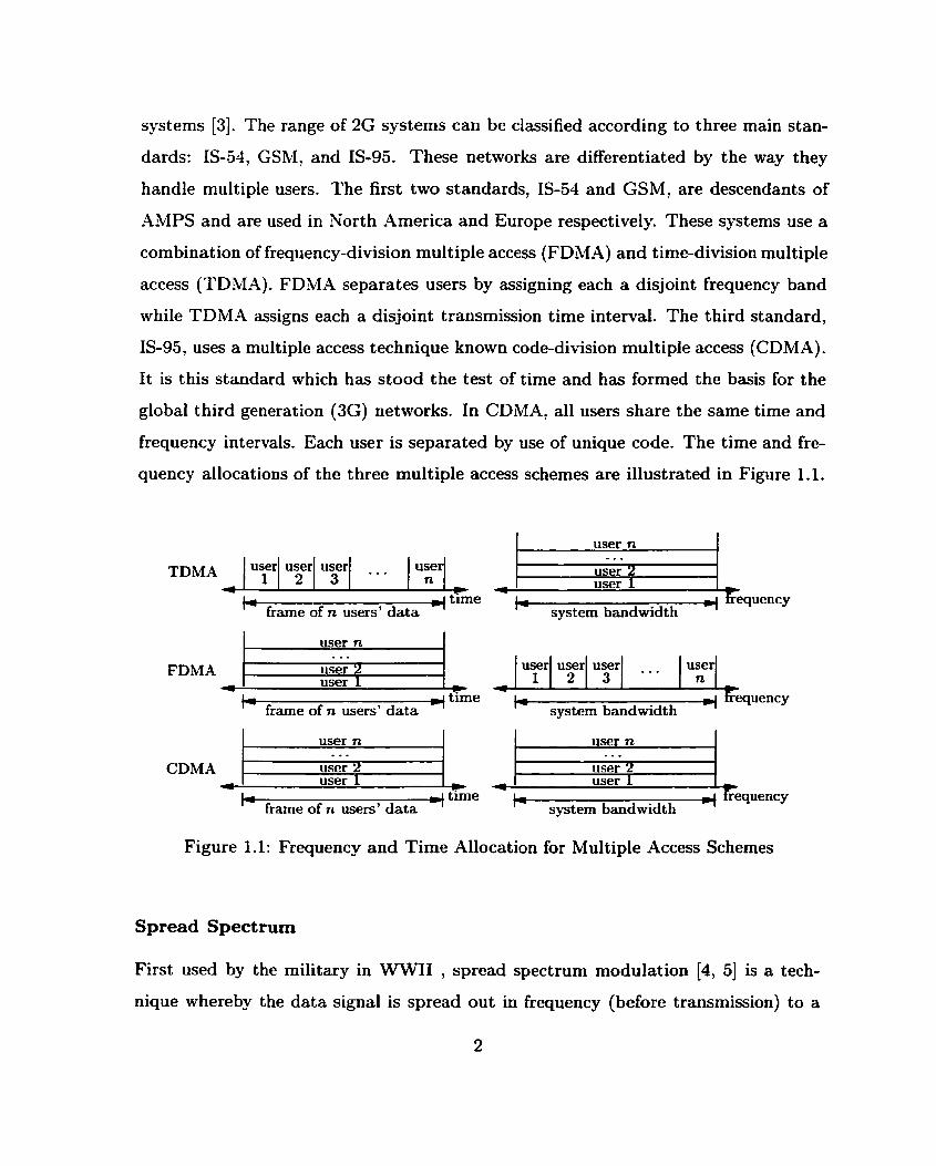
global third generation (3G) networks. In CDMA, al1 users share the same time and
frequency intervals. Each user is separated by use of unique code. The time and fre-
quency allocations of the three multiple access schemes are illustrated in Figure 1.1.
I user n I
I user n I
-. . user 2 user 1
TDMA
I user n I I user n I
t L '+ k system bandwidth
S . .
FDMA user 2 user 1
Figure 1.1: Frequency and Time Allocation for Multiple Access Schemes
user n
user
* time
frame of n users' data CI systembandwidth
CDMA
Spread Spectrum
First used by the military in W I I , spread spectrum modulation [4, 51 is a tech-
nique whereby the data signal is spread out in frequency (before transmission) to a
2
user n
user
. S .
user 2
user 1 2
r' user 1 time
frame of n users' data y
user 1 2 3
user 3
. - .
user - - -
bandwidth which is much larger than the signal data rate. This technique has an
inherent advantage over other communication strategies - it provides excellent inter-
ference rejection. This ability is due to the way the signal is spread out in frequency.
Of the many different type of spread spectrum, the two important ones are direct
sequence (DS) and frequency hopping (FH) . In frequency hopping, the data signal
is narrowband rnodulated but its carrier frequency is changed frequently (within a
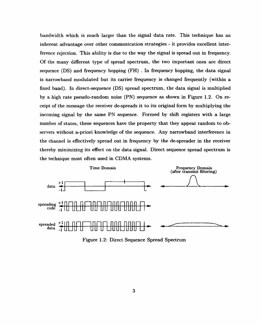
fixed band). In direct-sequence (DS) spread spectrum, the data signal is multiplied
by a high rate pseudo-randorn noise (PN) sequence as shown in Figure 1.2. On re-
ceipt of the message the receiver de-spreads it to its original form by multiplying the
incoming signal by the same P N sequence. Formed by shift registers with a large
number of states, these sequences have the property that they appear random to ob-
servers without a-priori knowledge of the sequence. Any narrowband interference in
the channel is effectively spread out in frequency by the de-spreader in the receiver
thereby minimizing its effect on the data signal. Direct sequence spread spectrum is
the technique most often used in CDMA systems.
Time Domain F'requency Doma@ (after transmit fil tering)
spreading +Io-- -
code
+ l - 1
Figure 1.2: Direct Sequence Spread Spectrum
data 4 -1- 1 L
I -
1.1.2 CDMA and Third Generation CeIlular Networks
CDMA was first proposed for cellular systems in 1978 [6] and was adopted for use in
IS-95. The telecommunications industry has recognized the merits of spread spectrum
and al1 proposed third generation standards specify the use of CDMA. The need for a
new standard is clear. The 2G networks with data rates of less than lOOkbps cannot
support the data rates required for internet traffic [ï]. Users want the flexibility of
global travel without having to worry about their terminal not being supported by
the local network; hence, a global standard is required. The first goal is realistic,
the second overly ambitious. In the end, two main global 3G CDMA standards were
developed: CDMA2000 and W-CDMA (81. The main reason for the development of
two unique standards was backwards-compatibility. In North America, much 1s-95
CDMA equipment is already in place. CDMA2000 was developed such that some
of this legacy equipment could be used. European and Japanese systems are not
restricted to backwards-compatibility since their 2G system is TDMAIFDMA based.
Their version of the 3G standard, known as wideband CDMA (W-CDMA) has many
similarities to the North American standard. The main difference lies in the choice
of chip rate. W-CDMA uses a rate of 3.098Mchips/s whereas CDMA2000 uses rates
which are multiples of 1.2288Mchips/s. Both however, aim to provide the same rates.
As a minimum, two different data rates are to be supported: 144kbps (with terminal
speeds of up to l20krn/h) and 2Mbps (with h e d terminal location). Also frame sizes
for data transmission are on the order of 10-20111s.
1.1.3 3G Channel. Considerations and Power Control
Third generation cellular networks are comprised of both downlink (forward) and u p
link (reverse) channels. On the downlink channels, the basestation is the transmitter
and the mobile users are the receivers. On uplink channels, the roles are reversed.
These channels are either located in disjoint frequency bands, known as frequency
division duplex (FDD) communication, or in disjoint time intervals, known as time
division duplex (TDD) communication. In the uplink, each mobile is assigned a dif-
ferent P N spreading (scrambling) sequence and communicates with the basestation
asynchronously (with respect to other mobiles). In the downlink of the 3G system,
transmission to al1 users is synchronous. Furthermore, each user's data signal is made
orthogonal to the others by assigning each an orthogonal spreading code. Upon re-
ception, hoivever, the data signals are no longer orthogonal. In communication over
wireless propagation environments, receivers tend to see multiple, delayed copies of
the transmitted signal. As a result, the orthogonality property of the signals is de-
stroyed. This causes severe problems (interference) for a user who is trying to decode
their intended received signal. There are several techniques which are used to mitigate
this effect. One way is through equalization. Each of these delayed copies (transmit
paths) contain valuable information about the data being transmitted. If received
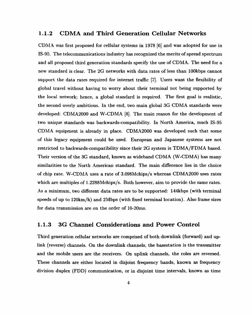
properly, the channel can be considered to exhibit time diversity. The Rake receiver,
introduced by Price and Green [9] in 1958 exploits this effect. I t is a technique used
a t the receiver to linearly equalize ISI in a multipath propagation environment. The
basic operation of the Rake receiver is as follows. A receiver will contain a set number
of 'fingers7. The purpose of these fingers is t o coherently receive (via a matched filter)
the paths with the best signal power. Each path is weighted and linearly combined to
produce the output signal, as shown in Figure 1.3. The second way this interference
problem is mitigated is through the use of power control. Each terminal or base sta-
tion adjusts its power, while maintaining the required performance level, such that
its interference-effect on other receivers is minirnized. This is done by attempting
to maintain a constant signal-to-noise (SNR) a t every receiver. In wireless channels,
keeping SNR constant is not easy Fading causes the constant transmitted signal
amplitude to Vary over time, thereby varying the SNR. The frequency of the fading
in a 3G propagation environment is on the order of 200Hz when moving a t a speed
of 120km/h and transmitting at a carrier frequency of 2GHz. While power control
information is sent to the receiver a t approximately 2kbps in 3G7 there is usually a
Figure 1.3: RAKE Receiver with n-fingers where h(t - ri) is the matched filter tuned to each path and wi(t) is scaling factor for each path
1-2 frame lag before the actual power is changed. As a result there is a range about
the average which the SNR will Vary over. Known as the fading rnargin, it is an
important consideration when determining the target (average) SNR. System perfor-
mance must not be compromised by these variations. As a result the channel coding
used must be both robust in this type of environment and, at the same time, provide
high spectral efficiency given a small frame size. Our work focuses on channel coding
techniques for the downlink which work well under these system and environmental
constraints. Coded modulation, and in particular bit-interleaved coded modulation,
is able to satisfies t hese constraints.
1.2 Bit-Interleaved Coded Modulation
The invention of trellis coded modulation(TCM) [IO] and multilevel coding [I l ] in the
1970's merged the principles of modulation and coding together into a single entity
which was appropriately called "coded modulation". These techniques provided sig-
nificant performance improvements in the bandwidth-limited regime of the additive
white Gaussian noise (AWGN) channel. Unfortunately, direct application of these
ideas to wireless fading channels does not result in the same performance improve-
ments [12]. Fading effectively causes errors which are bursty in time. Attempts
were made t o design new codes which employed a high degree of time diversity [12].
The objective of these codes is to interleave the symbols at a depth exceeding the
coherence time of the fading process. Zehavi [13] embraced this idea and proceeded
to take it one step further. In his approach, he recognized that performance could
be further improved by making the diversity equal to the number of bits rather than
the number of symbols along any error event. This diversity was achieved by bit-wise
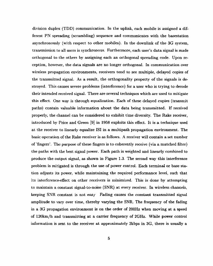
interleaving a t the encoder output. In a Iater publication, Caire et al. [14] named
this technique Bit-Interleaved Coded Modulation (BICM). A block diagram illustrat-
ing BICM is presented in Figure 1.4. In [14], a detailed theoretical analysis of the
BICM system was presented and it was proved that in terms of capacity, BICM is
sub-optimal to TCM.
/ CHANNEL (
DATA (IP?? )
VOICE??)
Figure 1.4: Bit-Interleaved Coded Modulation (BICM)
DATA 4
Despite its sub-optimality, BICM performs well in a fading channel. At a bit error
ENCODER MODULATOR
DECODER
* - BIT
INTERLEAVER
BIT DE-
INTERLEAVER
- DEMODULATORe

rate of Pb = 1 0 - ~ , BICM has been shown t o provide a SNR irnprovement of approxi-
mately 0.5dB when compared wit h symbol interleaved TCM [13] and approximately
1.2dB when compared to conventional multi-level coded modulation [15] over IID
Rayleigh channels. On AWGN channels, however, the performance using the same
codes is a t least 0.5 to 1dB worse than TCM and multi-level coding. This may be
explained by the fact t hat the bit-interleaving causes an inherent "random modula-
tion" [13] in the system which significantly reduces the free Euclidean distance. Li
and Ritcey [16] proposed a scheme which combats this effect. Their scheme, called
Bit-Interleaved Coded Modulation with Iterative Decoding (BICM-ID), utilizes iter-
ative decoding in combinat ion with hard-decision [16] or soft decision (1 71 feedback.
They have shown that these techniques can provide up to IdB improvement over
BICM in both AWGN and IID-Rayleigh environments.
1.3 This Work
The robustness of BICM to IID fading suggests that it may work well in a 3G propaga-
tion environment. Furthermore, turbo codes in combination with BICM may provide
the physical layer groundwork for a system which is not only robust t o fading and
multipath but performs well when compared to Shannon's capacity. This idea is the
underlying thread which binds together the work presented in this thesis. Specifically,
this thesis has several objectives:
1. To generate and analyze results for BICM over AWGN and IID Rayleigh Chan-
nels
O Generate capacity curves for BICM over AWGN and IID Rayleigh chan-
nels for various modulation schemes using different constellation mapping
techniques.
a Analyze the decoding complexity of BICM.
2. To generate and analyze results for BICM over a propagation environment which
exhibits Doppler fading and multipa.th propagation.
Analyze the 3G specs and develop a propagation mode1 which can easily
be implemented.
r Build an environment for simulation of Doppler and niultipath fading.
Generate and analyze results for BICM over one path slow and fast fading
propagation environments.
O Generate and analyze results for BICM over one path 3G slow fading
propagation environment.
O Generate and analyze results for BICM over a realistic 3G slow fading,
frequency select ive propagation environment.
3. To design an adaptive channel coding system for 3G wireless communications
using turbo codes.
O Design the adaptive rate strategy.
O Simulate a chosen turbo code in combination with BICM for various punc-
ture masks and modulation schemes.
O Select optimal configurations for use in the system and analyze perfor-
mance.
rn Analyze the decoding cornplexity of Turbo Codes in combination with
BICM.
This thesis begins, in Chapter 2, with an outline of the channels used. Chapter 3
introduces and analyzes BICM. The performance of BICM over wireless channels is
presented in Chapter 4 followed by the proposed adaptive BICM system in Chapter 5.
The thesis is summarized and future work is discussed in Chapter 6.
Chapter 2
Channel Models
When evaluating the performance of any proposed system, it is important to mode1
the system's environment as closely as possible. In this work, we examined perfor-
mance in a number of channel environments. This chapter will describe these channel
rnodels. They can be categorized into four types:
1. Additive White Gaussian Noise (AWGN) Channel
2. Independent Identically Distributed (IID) Rayleigh Fading Channel
3. Correlated Rayleigh Fading Channel (Flat Fading Channel)
4. Multipath, Correlated Rayleigh Channel (Frequency Selective Fading Channel)
The AWGN channel is well known [18, 19, 201 and will not be explained any further
here. The last three items are an intrinsic part of the wireless channel. They are
ordered by increasing complexity and will be described in Section 2.1.
2.1 Wireless Channels
When transmitting a signal over a wireless channel, the receiver will almost always see
multiple copies of the signal. These copies, varying in amplitude, phase, and possibly
frequency, will combine in a constructive or destructive manner a t the receiver. They
are due to reflections from the ground or man-made structures such as buildings. It
is the combinat ion of these received waves a t the receiver which results in small-scale
fading. Small-scale fading, often known simply as fading, will be the focus of this
section. There is another type of fading, known as large-scale fading, which deals
with the transmission of signals over large distances. Large-scale fading is typically
characterized by two effects: (i) free space propagation loss which is modelled as
the inverse mth power of distance and (ii) shadowing due to large structures such as
mountains which is modelled as the log normal distribution. For more information
on this type of fading see Rappaport [18].
Small-scale fading variations can be modelled by assuming that the transmitted
signal passes through a linear filter with a time varying impulse response. The impulse
response, h(t, T), completely characterizes the channel and is a function of both time
variations due t o motion, t, and channel multipath delay, T , for a fixed instance in
time. By convolving the transmitted signal, x(t), with the impulse response, h(t, T),
the signal which is present a t the receiver, y(t), can be determined. This received
signal, y(t), can be written as
where * is the convolution symbol and ~ ( t ) is AWGN with two sided power spectral
density &/2.
By assuming that the channel is band-limited and band-pass (as suggested by
Rappaport [18]), the impulse response, h(t , T), can be represented in terms of its
complex baseband (or low-pas) impulse response, hb(t, 7) .
where f, is the carrier frequency in Hertz (Hz).
-4long any one propagation path from the transmitter to the receiver, the signal
will be scaled by a complex fading envelope which varies in time and frequency.
Modelled as a single impulse, b(t - r ( t ) ) , the low-pas response can be written as
cT t ) hL-path (t, r ) = a( t , ~ ) e - j ~ * f ( ,
where a(t, T ) and ~ ( t ) are the amplitude and delay respectively.
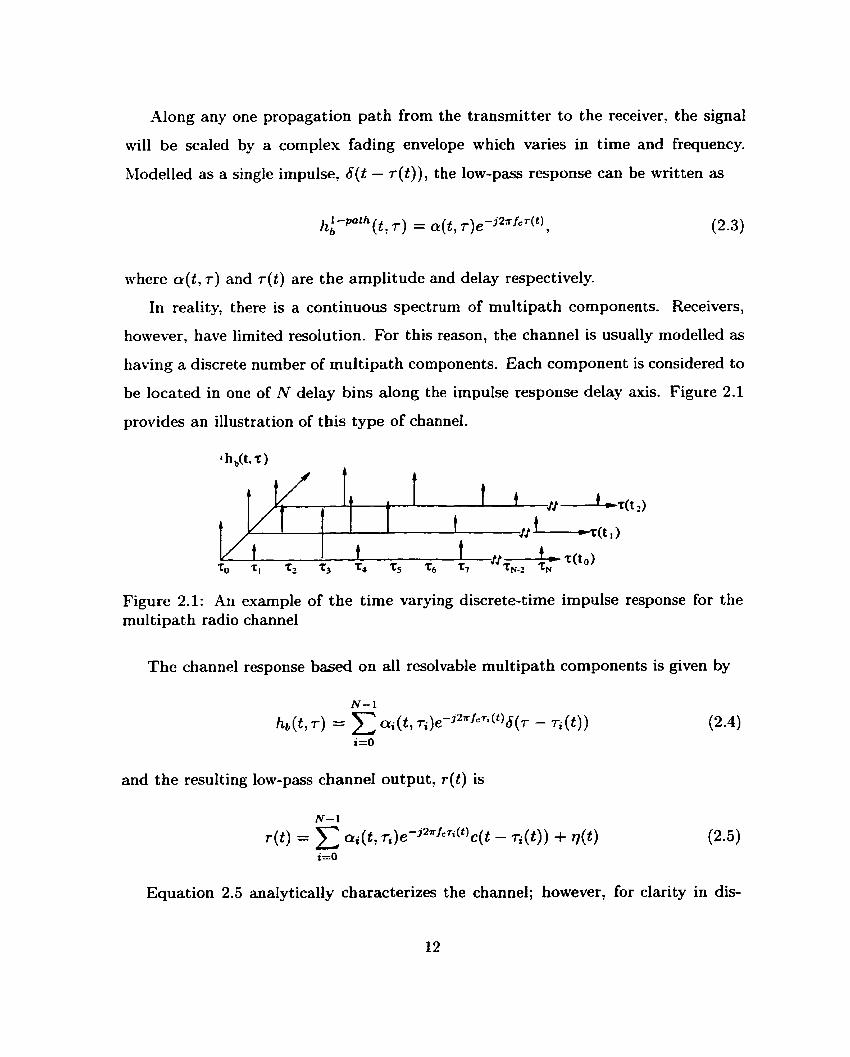
In reality, there is a continuous spectrum of multipath components. Receivers,
however, have limited resolution. For this reason, the channel is usually modelled as
having a discrete number of multipath components. Each cornponent is considered to
be located in one of N delay bins along the impulse response delay axis. Figure 2.1
provides an illustration of this type of channel.
Figure 2.1: An evample of the time varying discrete-time impulse response for the multipath radio channel
The channel response based on al1 resolvable multipath components is given by
and the resulting low-pass channel output, r(t) is
Equation 2.5 analytically characterizes the channel; however, for clarity in dis-
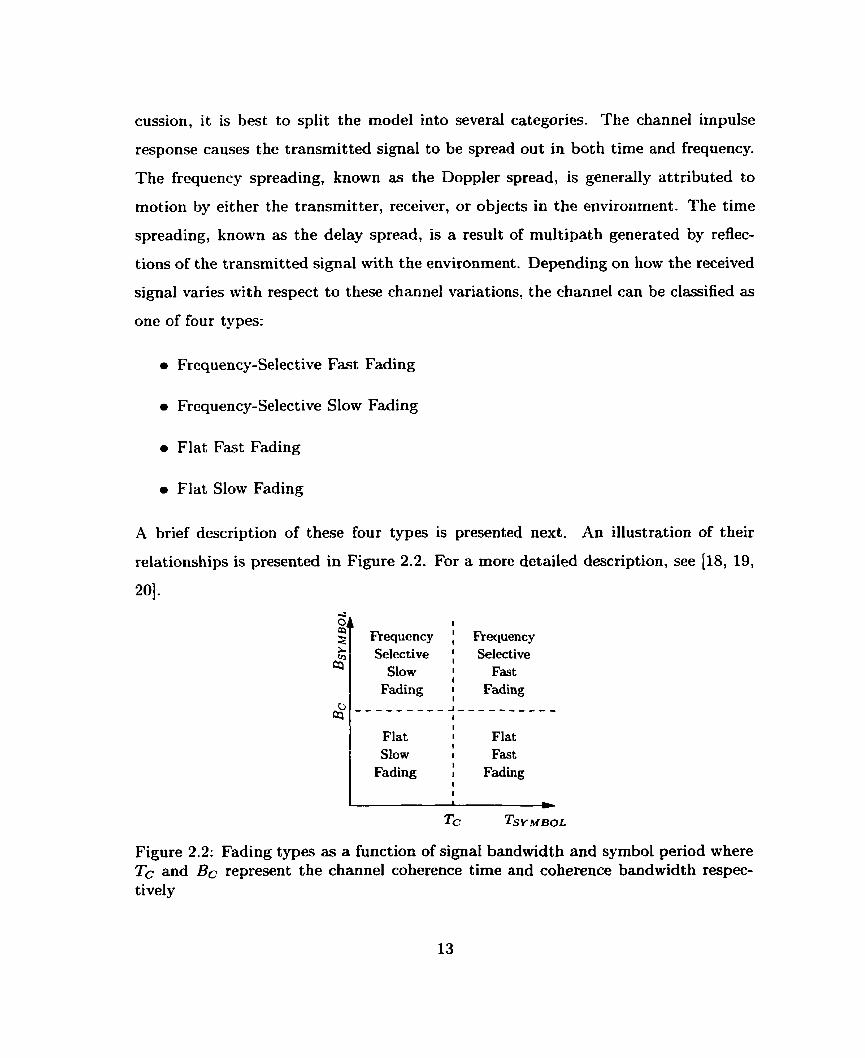
cussion, it is best to split the mode1 into several categories. The channel impulse
response causes the transmitted signal to be spread out in both time and frequency.
The frequency spreading, known as the Doppler spread, is generally attributed to
motion by either the transrnitter, receiver, or objects in the environment. The time
spreading, known as the delay spread, is a result of multipath generated by reflec-
tions of the transmitted signal with the environment. Depending on how the received
signal varies with respect to these channel variations, the channel can be classified as
one of four types:
O Frequency-Selective Fast Fading
O Frequency-Selective Slow Fading
0 Flat Fast Fading
O Flat Slow Fading
A brief description of these four types is presented next. An illustration of their
relationships is presented in Figure 2.2. For a more detailed description, see 118, 19,
201.
L
F'requency Selective
Slow Fading
- - - - - - - -
Flat Slow
Fading
I : Frequency Select ive
I Fast I 1 Fading
I I I Flat I I Fast
Fading t I
Figure 2.2: Fading types as a function of signal bandwidth and symbol penod where Tc and Bc represent the channel coherence time and coherence bandwidth respec- tively
Frequency-Selective Versus Flat Fading
If the channel induces no observable multipath components, the channel is considered
to be flat. This happens if al1 spectral components for a given signal see the same
channel characteristics (equal gain and linear phase). The rms delay spread is defined
as the standard deviation of the distribution of delays for a given received multipath
signal. It is a good indication of how much ISI will be induced by the channel. The
range of frequencies over which the channel is considered to be constant is known
as the coherence bandwidth (&). If the bandwidth of the signal is Larger than the
coherence bandwidth, frequency-selective fading will occur. Different portions of the
signal will be affected by the channel in different ways - inducing multipath effects.
Fast versus Slow Fading
Fast or slow fading is a measure of the rate at which the channel impulse response
varies with respect to the signal. The frequency of this variation is known as the
Doppler spread. If the Doppler spread is much less than the signal bandwidth, we
have slow fading. Otherwise, it is considered to be fast fading. Coherence bandwidth
was used to describe the range of frequencies over which the channel response was
invariant. A similar parameter is used here. The coherence time is defined as the
time interval over the channel response can considered constant.
Our work will examine the behavior of BICM over these four types of channels.
The flat fading channel (fast and slow) was implemented using Clarke's model [21]
and is discussed in Section 2.1.1 and illustrated in Figure 2.3. The frequency-selective
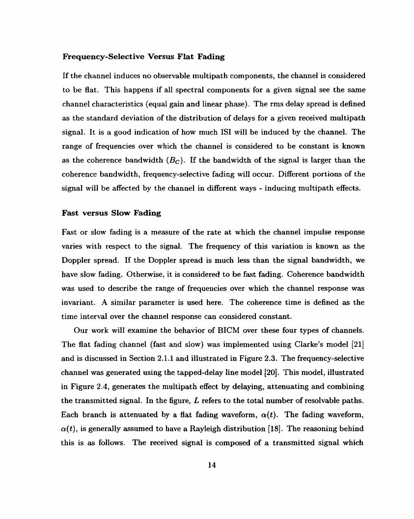
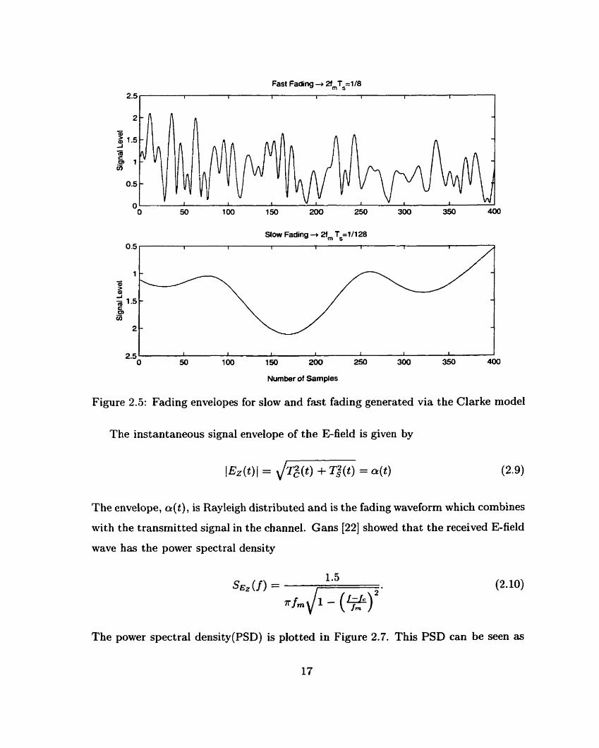
channel was generated using the tapped-delay line model [20]. This model, illustrated
in Figure 2.4, generates the multipath effect by delaying, attenuating and combining
the transmitted signal. In the figure, L refers to the total number of resolvable paths.
Each branch is attenuated by a flat fading waveform, <r(t). The fading waveform,
a(t), is generally assumed to have a Rayleigh distribution [18]. The reasoning behind
this is as follows. The received signal is composed of a transmitted signal which

has spread out in time. -4s stated above, the receiver resolves the received energy
into one or more paths. Each resolved path may be cornposed of multiple copies
of the transmitted signal, each slightly different in amplitude or phase. Using the
Central Limit Theorem [20], as the number of copies increases, the received signal
will assume a Gaussian distribution. The fading waveform is the envelope of the sum
of two quadrature Gaussian noise sources which is, by definition, a random variable
with a Rayleigh distribution. If there is motion by the receiver or transrnitter, a(t) is
generated using the Clarke model. If there is no motion whatsoever, a(t) is generated
using independent, identically, distributed(I1D) Rayleigh random variables.
Bot h Bat and frequency-selective channels can experience eit her slow or fast fading.
-4 convenient way to indicate the "speed" at which a channel is fading is by using
the normalized ratio 2 fm/ f, = 2 jmTs. The maximum Doppler shift, given in Hz,
is represented by fm and is equivalent to the velocity of the receiver relative to the
transmitter divided by the wavelength of the carrier frequency ( V I A ) . The bandwidth
and symbol period of the signal is represented by fs and Ts respectively. Figure 2.5
illustrate both slow and fast fading envelopes. Slow fading is generated using a
normalized ratio of 1/128 and fast fading was generated using 1/8. Both envelopes
were generated using the Clarke model.
Figure 2.3: Flat fading channel model
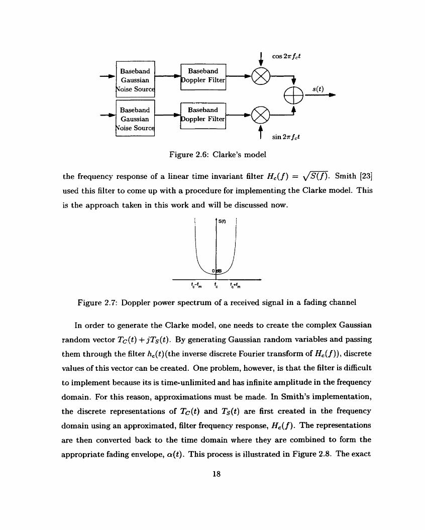
2.1.1 Clarke's Mode1 for Flat Fading
Clarke [21] stated that the electric field which is incident on the mobile is made up of
N randomly distributed plane waves (polarized in the same direction as the antenna).
Each wave has both a random arriva1 angle and a random phase. The electric field
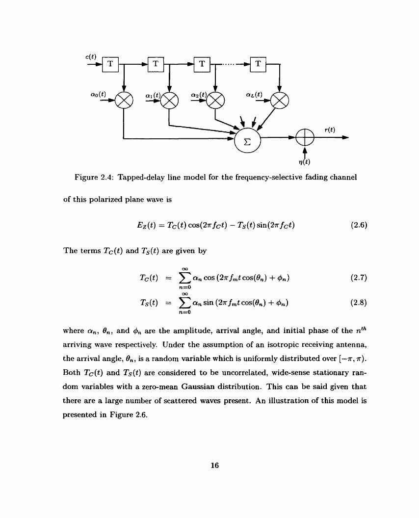
Figure 2.4: Tapped-delay line model for the freqüency-selective fading channel
of this polarized plane wave is
EZ (t) = Tc(t) cos(2a fct) - Ts(t) s i n ( 2 ~ fct)
The terms Tc(t) and Ts(t) are given by
Tc (t) = 1 an COS ( 2 ~ f,t cos(&) + 9,)
Ts(t) = an sin ( 2 ~ f,t cos(&) + &) n=O
where a,, O,, and 4, are the amplitude, arrival angle, and initial phase of the nth
arriving wave respectively. Under the assumption of an isotropic receiving antenna,
the arrival angle, On, is a random variable which is uniformly distributed over [-?r, a).
Both Tc(t) and Ts(t) are considered to be uncorrelated, wide-sense stationary ran-
dom variables with a zero-rnean Gaussian distribution. This can be said given that
there are a large number of scattered waves present. An illustration of this model is
presented in Figure 2.6.
Fast Fading 4 ZfmT9=1 18
2.5
2 - a2
1.5 J - m C 9 1 cn
0.5
O O 50 150 200 250 300 350 400
Stow Fading + 21, Ts=l/l 28
2.5 1 1 1 1 1 1 I 1 O 50 100 150 200 250 300 350 400
Number of Samples
Figure 2.5: Fading envelopes for slow and fast fading generated via the Clarke mode1
The instantaneous signal envelope of the E-field is given by
The envelope, a(t), is Rayleigh distributed and is the fading waveform which combines
with the transmitted signal in the channel. Gans [22] showed that the received Efield
wave has the power spectral density
The power spectral density(PSD) is plotted in Figure 2.7. This PSD can be seen as
s(t> 1111)
Baseband Baseband
sin 27r f,t
Figure 2.6: Clarke's model
the frequency response of a linear tirne invariant filter H,-( f) = d m . Smith [23]
useci this filter to come up with a procedure for implementing the Clarke model. This
is the approach taken in this work and will be discussed now.
Figure 2.7: Doppler power spectrum of a received signal in a fading channel
In order to generate the Clarke model, one needs to create the complex Gaussian
random vector Tc@) + jTs(t). By generating Gaussian random variables and passing
them through the filter h,(t)(the inverse discrete Fourier transform of Hc( f )), discrete
values of this vector can be created. One problem, however, is that the filter is difficult
to implement because its is time-unlimited and has infinite amplitude in the frequency
domain. For this reason, approximations must be made. In Smith's implementation,
the discrete representations of Tc(t) and Ts(t) are first created in the frequency
domain using an approximated, filter frequency response, Hc( f ). The representations
are then converted back to the time domain where they are combined to form the
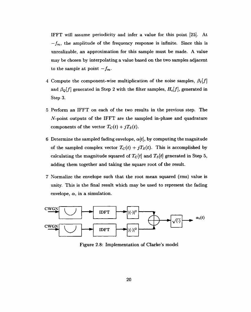
appropriate fading envelope, a@). This process is illustrated in Figure 2.8. The exact

procedure for generating iV sarnples of the envelope is a(t) is as follows:
1 Determine the values for the following parameters:
0 Carrier frequency ( j , ) - e.g. 2GHz
r Doppler frequency ( f , ) - e.g. for velocity= lZOkm/h, f, = =
222.22H.z where c is the speed of light
r Signal bandwidth (BW,) - e.g. 4.096iMHz
2 Generate N samples of complex white Gaussian noise in the frequency
domain for both the in-phase ( P l [ j ] ) and quadrature ( & [ f ] ) components
of the mode1 under the following constraints. The variables Tc(t) and
Ts(t) are real valued. This rneans that their frequency counterparts must
exhibit Hermitian symmetry. Also, given that the IDFT is
we can see X[k ] must be real valued when k = O and k = N / 2 in order
for x[n] to be real. The generated noise samples are effectively scaled
representations of these frequency counterparts and therefore must have
the same properties. Also, i t is recommended that N be a power of 2 such
that FFT algorithm can be used.
3 Generate S samples of the Doppler filter, H,[ f 1, where S is given by
According to Mahvidi [24], for accurate representation, the number of
samples, S, should be greater than 128. The samples are generated using
(2.10) with fc set to zero. They should be evenly distributed between
[- f,, + fm). It is not necessary to generate a sample for + fm since the
IFFT will assume periodicity and infer a value for this point [25]. At
- f,, the amplitude of the frequency response is infinite. Since this is
unrealizable, an approximation for this sample must be made. A value
rnay be chosen by interpolating a value based on the two samples adjacent
to the sample a t point - f,.
4 Compute the component-rvise multiplication of the noise samples, OI[f] and &[f] generated in Step 2 with the filter samples, H,[f], generated in
Step 3.
5 Perform an IFFT on each of the two results in the previous step. The
N-point outputs of the IFFT are the sampled in-phase and quadrature
cornponents of the vector Tc@) + jTs(t).
6 Determine the sampled fading envelope, a$], by computing the magnitude
of the sampled complex vector Tc(t) + jTs(t). This is accomplished by
calculating the magnitude squared of Tc[t] and Ts[t] generated in Step 5,
adding them together and taking the square root of the result.
7 Normalize the envelope such that the root mean squared (rms) value is
iinity. This is the final result which may be used to represent the fading
envelope, a, in a simulation.
Figure 2.8: Implementation of Clarke's mode1
IDFT Optimization
One problem with this implementation is that it is computationally expensive. The
effort required primarily has to do with performing the N-point IDFT. An FFT
algorithm is typically used to calculate the IDFT which requires roughly N log, iV
operations. When generating fading envelopes for 3G simulations, signal bandwidths
on the order of 4MHz (3.84Mcps) are used with Doppler filter bandwidths of approx-
imately 2Hz (3kM/h) 450Hz (l2Okm/h). In order to achieve good resolution on the
filter, an IDFT would have to be executed on sample sizes on the order of 106 points
or 20 bits (translating to 106 1 and Q filtered noise samples each). The FFT would
require approximately 20 million operations. This can prove to be very difficult to do
in real time. Furthermore, the number of noise samples which must be pre-generated
is large (2 million). While these may not be a large problem in software, a more effi-
cient way would be needed to implement such a mode1 in hardware (20 bit FFTs are
unrealistic). By modifying the implementation, the size of both the IDFT which must
be performed and the data which must be pre-generated can be reduced significantly.
The general formula for the IDFT is as follows:
There are two distinct properties exhibited by our frequency spectrum which can
be used to optimize the IDFT for Our application. They are as follows:
1. The spectrum appears as if it has been zero padded
2. The spectrum exhibits Hermitian symmetry X[f] = X*[- f]
The first property lets us redefine the IFFT such that the we sum over the non-zero
elements only
x, [kl index k -
..... 1-. ..... . ..
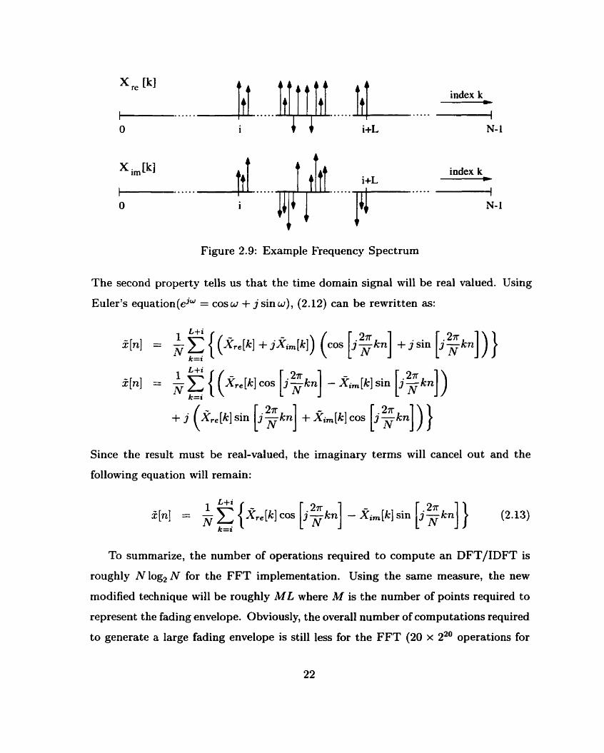
index k - Figure 2.9: Example Frequency Spectrum
The second property tells us that the time domain signal will be real valued. Using
Euler's equation(ejw = cos w + j sin w) , (2.12) can be rewritten as:
+ j (S.. [k] sin [ j kn] + &[k] cos j - kn [ N 1) ) Since the result must be real-valued, the imaginary terms will cancel out and the
following equation will remain:
L+i
- 1 C (8,. [k] cos [jg kn] - Xi , [k] sin +l - N k=i
To summarize, the number of operations required to c o m p t e an DFT/IDFT is
roughly N log, N for the FFT implementation. Using the same measure, the new
rnodified technique will be roughly ML where M is the number of points required to
represent the fading envelope. O bviously, the overall number of compu tations required
to generate a large fading envelope is still less for the FFT (20 x 2*" operations for
20 bit IDFT using FFT as opposed to 240 for the modified method). The advantage
of the method is that the a fading enveiope of any desired sample size can be easily
produced. This leads to less data storage at any one time, smaller IDFT, and &ter
computation.

Chapter 3
Bit-Interleaved Coded Modulation
Bit-interleaved coded modulation is a technique that combines coding, modulation,
and interleaving in a clever way such that the diversity of a communications system
is increased. It has been shown that while Euclidean distance is an important factor
in a ,4WGN channel, it is not so important in a fading channel [19]. What is more
important in these environments is diversity. Diversity is defined as the spreading
out of information across time or space. In the TCM type systems, the only way to
increase diversity is either increase the constraint length or to avoid parallel transitions
wi t hin the code. BICM , invented by Zehavi [l3], successfully increases diversity while
allowing for use of standard codes designed for the AWGN channel. This section will
describe the BICM system as well as the standard TCM system. The performance
of BICM will be examined over the AWGN and IID Rayleigh channel propagation
models.
3.1 BICM System Overview
In total the BICM system is comprised of three distinct elements: FEC coder/decoder,
interleaverlde-interleaver, and rnodulator/demodulator, as shown in Figure 3.1, which
depicts a BICM system using a rate-213 code with &PSK modulation. Although a

, - ), Interleaver - -
Rate 213 ci - - - - - - - - v; &PSK xt Encoder Interleaver
6;; -' Interleaver . cP r -
Pt
Figure 3.1: Zehavi's [13] BICM system using a rate-213 code with 8-PSK modulation
specific case is shown, BICM is flexible in allowing any type of code (punctured or
not) to be used in combination with virtuafly any modulation type. The best way to
understand BICM is by examining the encoder and decoder separatell
3.1.1 Encoder
1. The data bits are encoded using an (n, k) convolutional code such that
and
where Dp and Cp are the k-tuple of input bits and the n-tuple of encoded bits
of the p" input signal respectively. The labels d; and ci, represent the jth bit
of Dp and Cp respectively.

2. Each of the n outputs of the encoder is fed into an independent, random inter-
leaver .
3. Once interleaved, the binary n-tuple is mapped to one of 1V1 = Sn channel
signals in the signal set S where x = ~ ( v ' , v2, . . . , vn) and vi are the points in
the constellation. The constellation mapping used is Gray labelling for BICM
without iterative decoding [14] and mixed labelling for BIChd with iterative
decoding [26]. Three constellation mappings for &PSK are shown in Figure 3.2
and are described as follows:
Figure 3.2: BICM Gray, Set-partitioning, and Mixed labelling for 8PSK - the furthest bit to the right is the MSB
Gray labelling - The objective is to minimize the number of bit errors which
occur when a specific constellation point is transmitted but the receiver
thinks that the adjacent point has been sent. It can be thought of as
mavimizing diversity. This is done by assigning constellation points wit h
a binary representation which differs by only one bit between adjacent
points. For example in 8PSK, binary labels 101 and 111 are mapped to
adjacent points.
0 Set-partitioning (SP) labelling - The idea is to provide greatest protection
to the most significant bits and the least protection to the least significant
bits thereby rnaximizing effective Euclidean distance. This is done by
recursively splitting the constellation points in half, assigning each half to
the remaining most significant bits. For example in SPSK, al1 points which
have a label with a one as the MSB are adjacent to one another. No points
in which the LSB is one are adjacent to one another. In this scheme, if
the receiver again incorrectly chooses the adjacent point, there is a high
probability that the MSB will be correct.
0 Mixed labelling is a combination of both set-partitioning and Gray la-
belling. It is easiest to think of mixed labelling in reference to set parti-
tioning labelling. If b2, bi7 bo represents a binary label for natural labelling,
mixed labelling can be represented as b2, (q + b l ) , b0 and Gray labelling is
b2i (b + bi) , (bi + bo).
For example, the partitioning of the 8-PSK constellation into subsets for Gray
labelling is done as follows:
S = {x: z(k) = =exp ( j?) ,k = 0 ,1 , . . . ,6 ,7)
where S: is the constellation subset such that ith bit within the label has the
value b
4. The signal is then transmitted over the channel.
3.1.2 Decoder
1. The received signal is used to calculate two bit-metrics for each bit in the
n-tuple. For example, with 8-PSK, six bit-metrics are calculated a t each time
instant t . In conventional BICM, a sub-optimal b i t - m e t r i ~ , r n ~ ( ~ ~ , SP; p:), is used
instead of the optimal bit-metric, mi (y;, Sp; pf ) . This sub-optimal approxima-
tion of the optimal maximum-likelihood(ML) bit-metric, derived in Appendix A,
reduces the number of computational operations required for decoding. For
AWGN and Rayleigh channels, the bit-met rics are
A i b i mi(y t ,S i ;p t ) = - m i n I ( y t - z 1 ) 2 (AWGN)
ZES!
= -min II yt-ptx 11' (Rayleigh-Perfect CSI). ZES;
where Ot and pt are the amplitude and phase of the fading envelope a t time t
respect ively. The CS1 is the channel-st a t e informat ion and collect ively refers to
the channel affects on signal amplitude, phase, and delay. In AWGN, p:=l.
2. The trellis branch-metrics are then formed by de-interleaving and summing the
bit-metrics corresponding to al1 possible values of c'.
2 where Y, = (y;, y,, --- ,y:), p, = (pi, p:, -- -; pp), and the de-interleaved metrics
are written using the time sequence p instead of t. The symbol denotes an
estimated value.
3. The trellis branch-metrics are fed into the Viterbi decoder which determines the

binary sequence c with the highest cumulative surn of rnetrics.
where 1V represents the length of the codeword.
3.1.3 Iterative Decoder (BICM-ID)
In iterative decoding, the output of the decoder is fed back to the demodulator.
The demodulator uses the decoding information to help decide which point in the
constellation subset it should select. The exact procedure is as follows.
1. The first round of decoding using BICM-ID is identical to that of BICM.
3. The subsequent rounds of decoding al1 begin with this step. The iterative- I D i decoding bit-metric, mi (y,, S:; ph) , is re-calculated as follows for Rayleigh
channels with perfect CSI:
where 6: are the decoded bits out of the Viterbi decoder. A similar calculation
is performed for AWGN channels.
3. Branch-metric calculation - identical to the Step 2 for BICM (Section 3.1.2).
4. Viterbi decoding - identical to the Step 3 for BICM (Section 3.1.2).
Steps 2 and 3 above apply to hard-decision feedback only. Soft-decision feedback
employs the use of the BCJR algorithm over the trellis. More details on this decoding

strategy can be found in [17, 26, 271.
3.2 Performance
The performance of BICM is discussed in this section. We examine and contrast the
performance of BICM, BICM-ID and symbol-interleaved coded modulation (CM) over
various channels. The results in this section were simulated using a Rate 213, 8-state,
non-recursive convoIutiona1 code. This code is the same as the one used by Zehavi
(octal generators{(4,2,6,),(1,4,7)}) and is optimized for diversity [28, page 3311. The
simulations were run with a frarne size of 2502 bits and gray constellation labelling
was used for both CM and BICM. Mixed labelling was used for BICM-ID. A random
spread interleaver [29] was used which had a minimum spread of 26. Al1 performance
curves are presented in terms of bit-error rate(BER) versus normalized information
bit signal-to-noise ratio (SNR). The normatized bit SNR, in d B is determined by the
following relation
BitSNR = 10 log Es { = l0log{-) No R
where Eb, Es, and m are the average bit energy, average symbol energy, and number
of bits per symbol respectively. The code rate is represented by Rcode and the overall
rate is given by R. The AWGN noise power density, given by No is equal to twice
the variance of the AWGN noise(No = 2a2).
Figures 3.3 and 3.4 show the performance of the three schemes over the AWGN
and Rayleigh channels. These results confirm the results presented by Zehavi [13]
and by Li and Ritcey [26] over the same channels with thirteen decoding iterations.
Notice that for the .4WGN channel, CM always outperforms BICM. At a BER
. 4 5 . . . I . " . . ?- .
.I CM - BlCM . . '. -C BICM-ID
'. I I
1 2 3 4 5 6 7 B (a)
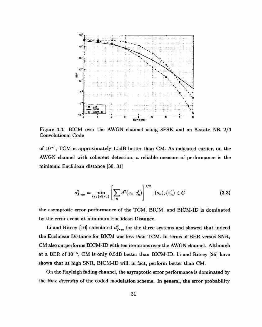
Figure 3.3: BICM over the AWGN channel using 8PSK and an 8-state N R 213 Convolut ional Code
of 1 0 - ~ , TCM is approximately 1.5dB better than CM. As indicated earlier, on the
AWGN channel with coherent detection, a reliable measure of performance is the
minimum Euclidean distance [30, 311
d&,, = min
the asymptotic error performance of the TCM, BICM, and BICM-ID is dominated
by the error event a t minimum Euclidean Distance.
Li and Ritcey [16] calculated d2/,, for the three systems and showed that indeed
the Euclidean Distance for BICM was less than TCM. In terms of BER versus SNR,
CM also outperforms BICM-ID wit h ten iterations over the AWGN channel. Although
at a BER of CM is only 0.5dB better than BICM-ID. Li and Ritcey [26] have
shown that a t high SNR, BICM-ID will, in fact, perform better than CM.
On the Rayleigh fading channel, the asymptotic error performance is dominated by
the tzme diversity of the coded modulation scheme. In general, the error probability
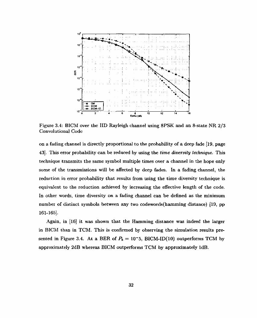
Figure 3.4: BICM over the IID Rayleigh channel using 8PSK and an 8-state NR 213 Convolut ional Code
on a fading channel is directly proportional to the probability of a deep fade (19, page
431. This error probability can be reduced by using the time diversity technique. This
technique transmits the same symbol multiple times over a channel in the hope only
some of the transmissions will be affected by deep fades. In a fading channel, the
reduction in error probability that results from using the time diversity technique is
equivalent to the reduction achieved by increasing the effective length of the code.
In other words, time diversity on a fading channel can be defined as the minimum
number of distinct symbols between any two codewords(hamming distance) [19, pp
Again, in [16] it was shown that the Hamming distance was indeed the larger
in BICM than in TCM. This is confirmed by observing the simulation results pre-
sented in Figure 3.4. At a BER of Pb = 10-5, BICM-ID(10) outperforms TCM by
approximately 2dB whereas BICM outperforms TCM by approximately 1dB.

Figure 3.5: BICM over the AWGN channel using an 8-state NR 2/3 Convolutional Code
3.3 Capacity
Capacity is a measure of the amount of information which can be reliably sent over a
given channel. Shannon showed that the capacity of a discrete, memoryless channel
is given by:
C = max I (x; y), P(Z)
where p(x) is the input distribution and I(x; y) is the mutual information between
two random variables, x and y [32]. The capacity of coded modulation was derived
by Ijngerboeck [ ID]. Under the constraint of uniform input distribution, it can be
written (in terms of information bits per N complex dimensions) as
where x, y and 8 are the input, output and the channel state parameters respectively.
The transition pdf is represented by pe( ). S is the channel signal set and m = log, ISI.
In BICM, the interleaver has the effect of creating m parallel independent channels

over which the data is transmitted (141. The capacity becomes the average of the
AMI'S for each of the rn independent channels. The resulting capacity for BICM
with perfect CS1 and uniforni inputs is
By means of the data-processing theorem [32, page 321, they proved that
Furthermore, Caire et al. [14, 331 used (3.5) to develop capacity curves for QPSK,
8-PSK and 16QAM BICM with SP and Gray labelling. We have regenerated the
curves and have included capacity with mixed labelling. Note that mixed labelling
is equivalent to S P labelling for QPSK and 16QAM These curves are shown in Fig-
ures 3.6 through to and 3.11. The curves have been generated by collecting 2048 noise
samples a t each point. It can easily be observed from the figures that performance
of BICM using Gray labelling is the best and is very close to that of CM. In fact, it
is equal to CM for QPSK. Mixed labelling performs better that SP for BPSK. Mixed
labelling is the same as SP for QPSK and 16QAiM.
3.4 BICM Complexity
In Appendix D, we derive the complexity involved in decoding BICM, TCM, and
BICM-ID using convolutional codes. If we define the total number of operations
required for decoding TCM as H, then by using a rough approximation of the equa-
tions in Tables D.7-D.4, it can be said that the total number of operations required
for Rayleigh decoding of BICM is (2M) H for the optimal metric and (1 .5M)H for the
sub-optimal metric when using convolutional codes where M represents the number
of signals in the constellation. For Rayleigh decoding of BICM-ID, the total number
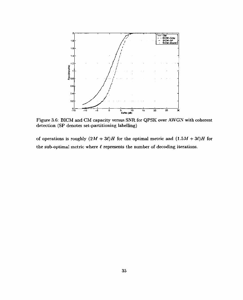
Figure 3.6: BICM and CM capacity versus SNR for QPSK over AWGN with coherent detection (SP denotes set-partitioning labelling)
of operations is roughly (2M + 3e)H for the optimal metric and (1.5M + 3e)H for
the sub-optimal metric where l? represents the number of decoding iterations.

Figure 3.7: BICM and CM capacity versus SNR for QPSK over Rayleigh fading with coherent detection (SP denotes set-partitioning labelling)
Figure 3.8: BICM and CM capacity versus SNR for &PSK over AWGN with coherent detection (SP denotes set-partitioning labelling)

Figure 3.9: BICM and CM capacity versus SNR for 8-PSK over Fiayleigh coherent detection (SP denotes set-partitioning labelling)
Figure 3.10: BICM and CM capacity versus SNR for 16-QAM over with perfect CS1 (SP denotes set-partitioning labelling)
fading with
AWGN fading
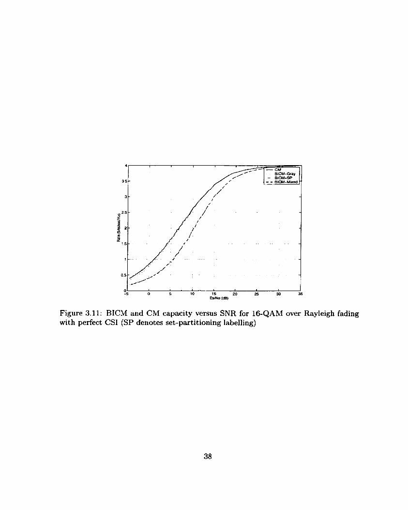
Figure 3.11: BICM and CM capacity versus SNR for 16-QAM over Rayleigh fading with perfect CS1 (SP denotes set-partitioning labelling)

Chapter 4
3G Wireless C hannels
This chapter will examine the performance of BICM in a 3G wireless type channel.
The sections in this chapter will detail the selected 3G channel model, briefly discuss
spreading and the Rake receiver, and present the results of the multipath simulations.
First , however, BICM will be examined in a single-propagation environment.
4.1 Single-Pat h (Frequency Non-Selective) Perfor-
mance
Before performance of BICM in multipath is analyzed, it is useful to first examine the
single-path case. Single-path propagation in a wireless channel is also referred to as
frequency non-selective propagation. Figure 4.1 shows the performance of BICM in
a single-path environment for both slow and fast fading conditions. The first obser-
vation which can be made is that BICM outperforms CM with symbol-interleaving
by almost an order of magnitude a t an SNR of 14dB. The BER for BICM is roughly
2 x 10⁻⁵ when CM with symbol interleaving has a BER of 1 0 - ~ . Furthermore, it
can be readily seen that BICM exhibits the same performance for both fast and slow
fading. This may be attributed to the fact that the block length is relatively small
(2502 bits), which limits the distance which the bits can be separated. Small block
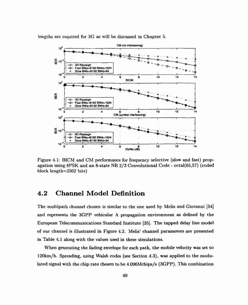
lengths are required for 3G as will be discussed in Chapter 5 .
CM (no interleaving) loO , I I 1 1 1
a
+ Fast BWs=8192 BWd=1024 Slow BWs=8192 BWd=64
CM (symbol interleaving) loO l I 1 I I 1 I I
7 IIU nayiuiyri ' + Fast BWs-8
x Slow BWs=8192 BWd64 1 *na-' 1 I I 1
'" O 2 4 6 8 1 O 12 14 EhMo (dB)
Figure 4.1: BICM and CM performance for frequency selective (slow and fast) p r o p agation using 8PSK and a n 8-state NR 213 Convolutional Code - octa1(65,57) (coded block length=2502 bits)
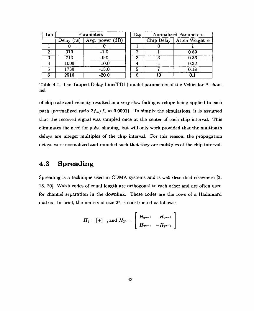
4.2 Channel Mode1 Definit ion
The multipath channel chosen is similar to the one used by Melis and Giovanni [34]
and represents the 3GPP vehicular A propagation environment as defined by the
European Telecommunications Standard Institute [35]. The tapped delay line mode1
of our channel is illustrated in Figure 4.2. Melis' channel parameters are presented
in Table 4.1 along with the values used in these simulations.
When generating the fading envelope for each path, the mobile velocity was set to
120km/h. Spreading, using Walsh codes (see Section 4.3), was applied to the modu-
lated signal with the chip rate chosen to be 4,09GMchips/s (JGPP). This combination

f 0.89ai (t)
r u ) 'r~ = 3 chip
m
I t 0.36az(t)
O. 18ar ( t )
Figure 4.2: Tapped Delay Line Mode1 Used in Simulations
I T ~ P I Paramet ers I 1 T ~ P 1 Normalized Parameters 1 t
1
Table 4.1: The Tapped-Delay Line(TDL) mode1 parameters of the Vehicular A chan- ne1
L
1 Delay (ns)
O
of chip rate and velocity resulted in a very slow fading envelope being applied to each
path (normalized ratio 2 f,/ f, x 0.0001). To simply the simulations, it is assumed
that the received signal was sampled once a t the center of each chip interval. This
eliminates the need for pulse shaping, but will only work provided that the multipath
delays are integer multiples of the chip interval. For this reason, the propagation
delays were normalized and rounded such that they are multiples of the chip interval.
Avg. power (dB) O
4.3 Spreading
Chip Delay O
Spreading is a technique used in CDMA systems and is well described elsewhere [3,
18, 201. Walsh codes of equal length are orthogonal to each other and are often used
for channel separation in the downlink. These codes are the rows of a Hadamard
matrix. In brief, the matrix of size 2" is constructed as follows:
Atten Weight a 1
H2n-L H2n-1 H I = [+] , and Hz. =
Hz*-1 -H2n-i J
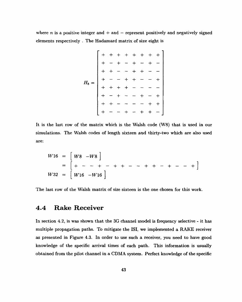
where n is a positive integer and + and - represent positively and negatively signed
elements respectively . The Hadamard matrix of size eight is
It is the last row of the matrix which is the Walsh code (W8) that is used in our
simulations. The Walsh codes of length sixteen and thirty-two which are also used
are:
The last row of the Walsh matrix of size sixteen is the one chosen for this work.
4.4 Rake Receiver
In section 4.2, is was shown that the 3G channel mode1 is frequency selective - it has
multiple propagation paths. To rnitigate the ISI, we implemented a RAKE receiver
as presented in Figure 4.3. In order to use such a receiver, you need to have good
knowledge of the specific arriva1 times of each path. This information is usually
obtained from the pilot channel in a CDMA system. Perfect knowledge of the specific
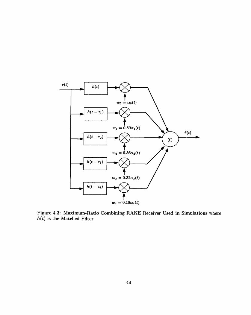
Figure 4.3: Maximum-Ratio Combining RAKE Receiver Used in Simulations where h(t) is the Matched Filter

path delays will be assumed in our irnplementation. Once ail the paths are coherently
tuned, there is still the question of how to combine them. There are several types of
combining strategies - the two major ones being: maximum-ratio combining (MRC)
and equal-gain combining (EGC) [18]. Equal-gain combining wveights al1 paths equally
and coherently adds tbem together. Maximum-ratio combining, shown to be the
optimal linear combining strategy [36, 371, wveighs each of the fingers by their channel
a t tenuation. The obvious requirement for this met hod is that good amplitude channel
state information is required. Like delay, this measurement is often performed on the
pilot signal. In a 3G propagation environment, the fading envelope changes slowly;
therefore, i t is relatively easy to make this measurement. For this reason, wve will
assume perfect amplitude channel state information and will use the maximum-ratio
combining technique.
4.5 Mult ipat h (Frequency Select ive) Performance
In this section, the performance of BICM is examined in a multipath environment.
Figures 4.4, 4.5, 4.6, and 4.7 illustrate the performance in two multipath channel
configurations. The channels and Rake receivers used are 3-path/%finger and 5-
path/5-finger models based on the UMTS model shown in Figure 4.2. The 3-path/3-
finger mode1 only used the first three taps of the UMTS model. The data is encoded,
modulated and then spread with the length 16 Walsh code as described in Section 4.3.
There are several observations which can be made from these figures. The most
important of which is that bit-interleaving provides the same performance when com-
pared to symbol-interleaving over the 3-Path channel and, in fact, provides worse
performance over the 5-Path channel. This result supports the theory that as the
number of resolvable paths increases, the channel begins to appear more and more
Gaussian-like [19]. As shown in Section 3.2, bit interleaving performs better than
symbol interleaving over a Rayleigh channel but worse over an AWGN channel. The

Figure 4.4: BICM over the bpath, multipath fading channel using a 3-finger RAKE receiver with perfect CS1 for 8PSK using an 8-state NR 213 Convolutional Code - octa1(65,57)
second interesting effect is the 16-QAM error floor in Figure 4.7. This error floor can
be attributed to the autocorrelation properties of the Walsh spreading code (shown in
Figure 4.8). We see from the figure that the correlation of the sequence with shifted
versions of itself is relatively high. It appears that this may induce an error floor at
high SNRs. We also observed that as the spreading factor becomes larger relative to
the delay spread of the channel, the error floor begins to appear at higher SNRs. To
mitigate this effect, one would need to either increase the spreading factor or use a
better code and/or interleaver. In the next section we will explore the use of turbo
codes in such a system.
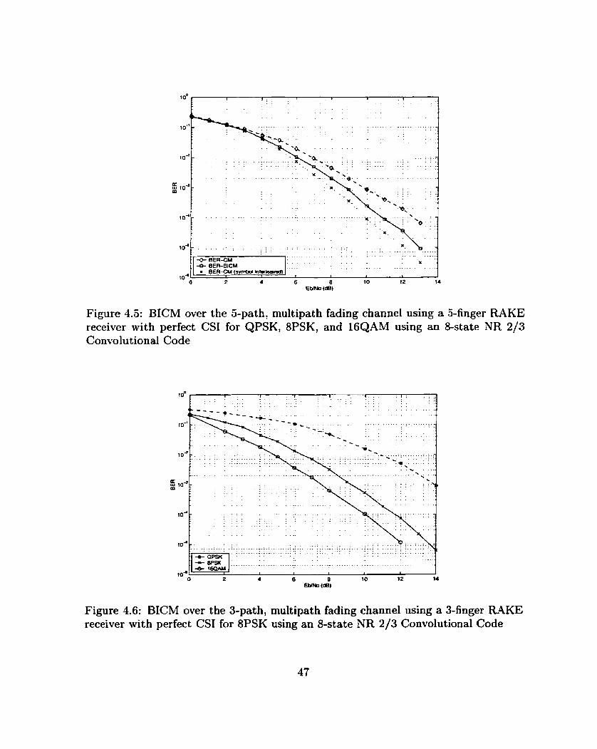
Figure 4.5: BICM over the 5-path, multipath fading channel using a 5-finger RAKE receiver with perfect CS1 for QPSK, BPSK, and 16QAM using an 8-state NR 2/3 Convolut ional Code
Figure 4.6: BICM over the 3-path, multipath fading channel using a 3-finger RAKE receiver with perfect CS1 for 8PSK using an 8-state NR 2/3 Convolutional Code

Figure 4.7: BICM over the 5-path, multipath fading channel using a 5-finger RAKE receiver with perfect CS1 for QPSK, 8PSK, and QPSK using an û-state NR 213 Convolut ional Code
Figure 4.8: Autocorrelation of Walsh 16 spreading code of length 16
Chapter 5
Adaptive 3G Channel Coding
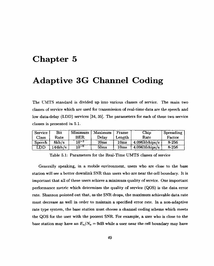
The UMTS standard is divided up into various classes of service. The main two
classes of service which are used for transmission of real-time data are the speech and
low data-delay (LDD) services [34, 351. The parameters for each of these two service
classes is presented in 5.1.
Table 5.1: Parameters for the Real-Time UMTS classes of service
Generaliy speaking, in a mobile environment, users who are close to the base
station will see a better downlink SNR than users who are near the ce11 boundary. It is
important that al1 of these users achieve a minimum quality of service. One important
performance metric which determines the quality of service (&OS) is the data error
rate. Shannon pointed out that, as the SNR drops, the maximum achievable data rate
must decrease as well in order to maintain a specified error rate. In a non-adaptive
rate type system, the base station must choose a channel coding scheme which meets
the QOS for the user with the poorest SNR. For example, a user who is close t o the
base station rnay have an EJN, = 9dB while a user near the ce11 boundary may have
Service Class
Speech LDD
Chip Rate
4.096hIchips/s 4.096Mchips/s
Bit Rate 8kb/s
144kb/s
Spreading Factor 8-256 8-256
Frarne Length lOms 10ms
Minimum BER 10-~ 10-~
Maximum Delay 20ms 50ms
an Es/No = 3dB. The maximum achievable rates for these SNRs are 3.16 bits/s/Hz
and 1-58 bits/s/Hz respectively. If the base station is forced to select a channel coding
scheme which accommodates the worse of the two SNRs, the user close to the base
station will have their ma.ximum available data rate cut in half. One solution to
mitigate this problem is to have an adaptive channel coding scheme which is based
on the user's SNR.
In this chapter, an adaptive channe1 coding scheme based on BICM using a 16-
state turbo code for the two UMTS classes of service is proposed. For each class of
service, a set of configurations (consisting of various code rates and modulation types)
will be selected which will guarantee system rate performs within a fixed distance
from capacity over a range of SNRs. The turbo code used is explained in detail in
Appendix B.
5.1 Service Class Constraints
In an UMTS system, the two classes of service mentioned above would exist on two
different types of data (traffic) channels. Typically, in the downlink, a user would be
assigned one or more traffic channels which would carry voice and/or IP type traffic.
The speech channel would carry voice (or latency intolerant) type traffic whereas
the LDD channel would carry IP (or latency tolerant) type traffic. These channels
would be made orthogonal to each by assigning each channel a different orthogonal
spreading code (usually a diBerent row of the Walsh matriv which as described in
Section 4.3).
In the LDD class of service, a delay of up to 50ms can be tolerated. The BER,
however, must be less than One way to achieve this is t o use selective-repeat
ARQ. This topic is well discussed in the literature (see [38, 39, 291) and will be
briefly described here. Simply stated, the transmitter(base station) continuously
sends frames of coded data to the receiver(user terminal). Before turbo encoding
in the transmitter, each frame will have been CRC encoded. The CRC bytes will
have been appended to the data entering the turbo code. As the receiver decodes
the frames, a CRC check will be executed. If the frame fails the check, the receiver
will prompt the transmitter to send the corrupt frame again. As discussed, with
turbo codes, an error floor will tend to appear a t lower BERS. This problem can be
mitigated through the choice of a better interleaver [40]. With the spread interleavers
used in this work, the error floor appears a t approximately For this reason, the
selective-repeat ARQ is a viable option for thr: LDD channel. An ARQ scheme will
attempt to keep the data error rate a t zero. In order to satisfy this strategy, there can
be no bound on the number of retries allowed. In reality, however, there is a bound
and in the LDD class the bound is chosen such that the overall latency is less than
.50ms. When using an ARQ scheme, there are two questions which must be answered.
First, what should the FER operating point be? By choosing the minimum raw FER
to be a BER of roughly IOd4 can be achieved. Second, what is the maximum
allowable number of retries? With a delay tolerance of 50ms and assuming there is
some processing time associated with an ARQ request, a choice of a maximum three
retries of lOms frames would be appropriate. Given these set tings, the corresponding
post-ARQ FER would be roughly with a BER of 10-12. This scheme fulfills the
requirements of the LDD class of service and will be basis for choosing a set of LDD
operating configurations.
Unlike the LDD class, the speech service class cannot tolerate latency. It can,
however, tolerate a reasonably high BER of This means that, with a frame size
of lOms and a maximum delay of 20ms, there is only enough time to send one block
of data. Based on this constraint, a similar set of operating configurations will be
chosen for the speech class.
5.2 LDD and Speech Class Operating Modes
The simulations which are used as the b a i s for selection of operating modes as per-
formed over an AWGN channel. The motivation for this is as follows.
5.2.1 AWGN Propagation Selection
There are two major differences between traffic channels which experience AWGN
only and ones which experience both AWGN and frequency-selective fading (see Chap-
ter 4). The first is that the data transmission in 3G must contend with varying SNR
due to the fading. In a slow fading channel such as one experienced in 3G systems,
the Doppler bandwidth is approximately 3Hz and 200Hz for motion of 3km/h and
12Okmlh. In 3G, the power control updates happen at 1500Hz - much faster than the
fading rate. This means tha t assuming that we are able to obtain good channel state
estimates, power control will mitigate the fading and the SNR will be kept constant
a t the receiver. The other significant difference is the multipath propagation. By
employing a RAKE structure in the receiver, the self-interference caused by multi-
path and, for that matter, multiple access interference can be modelled as AWGN
noise. . Furthermore, we demonstrated that the performance of BICM in multipath
fading is more like the AWGN performance than the performance in single path,
Rayleigh propagation. Based on these assumptions we can Say that the combination
of the RAKE receiver with fast power control makes the multipath, fading channel
conditionally Gaussian. As a result, it makes more sense to design the system around
simulations performed in an AWGN environment.
5.2.2 Selection of Modes
The operating modes were drawn from a set of eighteen configurations which included
a 16-state turbo code punctured to six different rates (113, 2/5, 419, 1/2, 2/3, and
4/5) and three modulation schemes with three different spectral efficiencies (2, 3,
and 4 bits/symbol/2D). From these eighteen combinations of modulation and code
rates, ten different operating modes were selected - providing channel coding rates
ranging from 2/3 up to 1615 bits/symbol/2D. The turbo code and puncturing masks
used are described in Appendk B. The modulation consisted of three Gray mapped
constellations - namely QPSK, 8PSK, and 16QAM with spectral efficiencies of 2; 3;
and 4 bits/symbol/2D respectively. Detailed performance curves for al1 the puncture
masks and modulations are presented in Appendix C
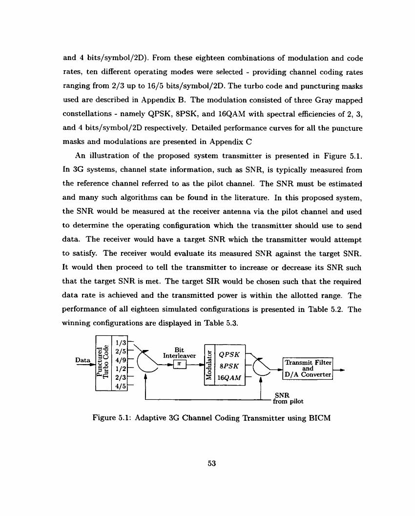
An illustration of the proposed system transmitter is presented in Figure 5.1.
In 3G systems, channel state information, such as SNR, is typically measured from
the reference channel referred to as the pilot channel. The SNR must be estimated
and many such algorithms can be found in the literature. In this proposed system,
the SNR would be measured a t the receiver antenna via the pilot channel and used
to determine the operating configuration which the transmitter should use to send
data. The receiver would have a target SNR which the transmitter would attempt
to satisfy. The receiver would evaluate its measured SNR against the target SNR.
It would then proceed to tell the transmitter to increase or decrease its SNR such
that the target SNR is met. The target SIR would be chosen such that the required
data rate is achieved and the transmitted power is within the allotted range. The
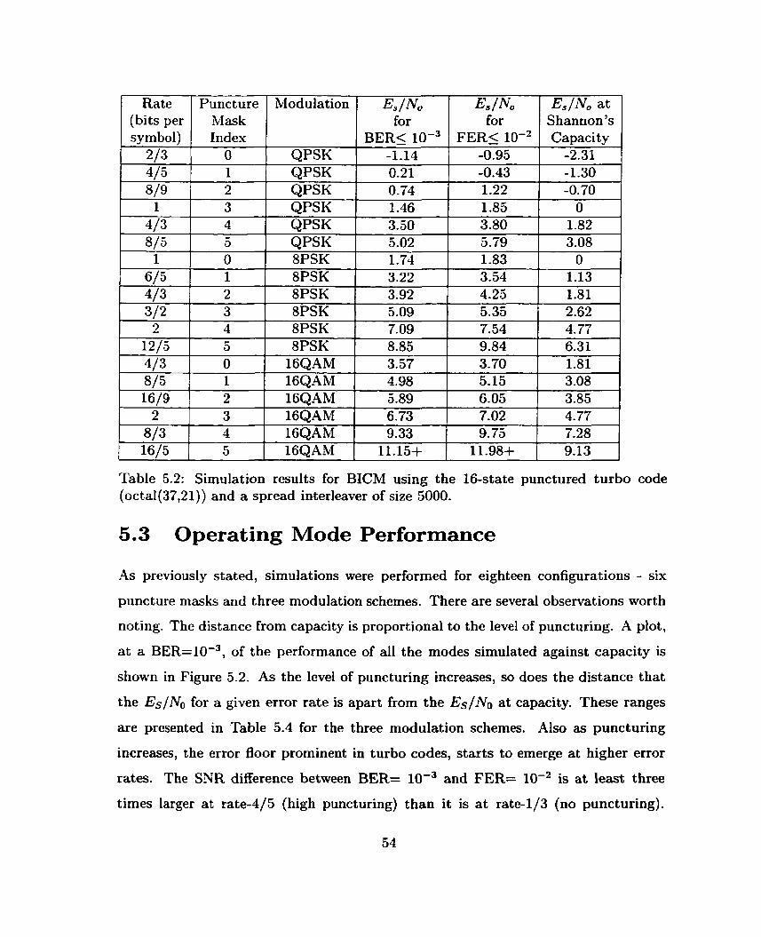
performance of al1 eighteen simulated configurations is presented in Table 5.2. The
winning configurations are displayed in Table 5.3.
QPSK
BPSK
16QAM
t fzp i lo t
Figure 5.1: Adaptive 3G Channel Coding Transmitter using BICM
Rate (bitsper symbol)
2/3 4/5 8/9
Table 5.2: Simulation results for BICM using the 16-state punctured turbo code (octa1(37,21)) and a spread interleaver of size 5000.
Puncture Mask
4/3 8/5 1
5.3 Operating Mode Performance
&/No at Shannon's
Index O 1 2
As previously stated, simulations were performed for eighteen configurations - six
puncture rnasks and three modulation schemes. There are several observations worth
noting. The distance from capacity is proportional to the level of puncturing. A plot,
a t a BER=10-3, of the performance of al1 the modes simulated against capacity is
shown in Figure 5.2. -4s the level of puncturing increases, so does the distance that
the Es/No for a given error rate is apart from the Es/& at capacity. These ranges
are presented in Table 5.4 for the three modulation schemes. Also as puncturing
increases, the error floor prominent in turbo codes, starts to emerge at higher error
rates. The SNR difference between BER= 10-~ and FER= IO-* is at least three
times larger at rate-4/5 (high puncturing) than it is a t rate-1/3 (no puncturing).
ESIN for
Modulation
4 5 O
EJN, for
QPSK QPSK QPSK
QPSK QPSK 8PSK
BERS 10-~ -1.14 0.21 0.74
3.50 5.02 1.74
FERS -0.95 -0.43 1.22
Capacity -2.31 -1.30 -0.70
3.80 5.79 1.83
1.82 3.08
O
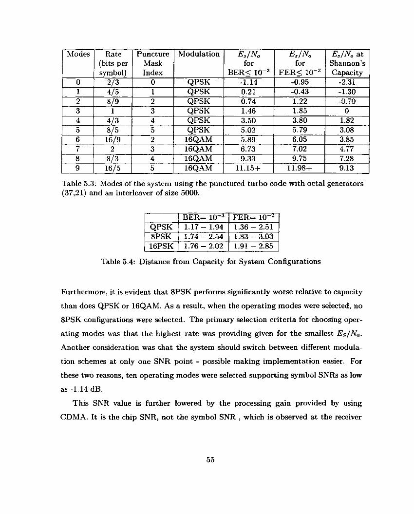
Table 5.3: Modes of the system using the punctured turbo code with octal generators (37'21) and an interleaver of size 5000.
QPSK 1 1.17 - 1.94 1 1.36 - 2.51 1 1 I
-Modes
O 1 2 3
-- - - -- -
Table 5.4: Distance from Capacity for System Configurations
Modulation
QPSK QPSK QPSK QPSK
Furthermore, it is evident that 8PSK performs significantly worse relative to capacity
than does QPSK or 16QAM. As a result, when the operating modes were selected, no
8PSK configurations were selected. The primary selection criteria for choosing oper-
ating modes was that the highest rate was providing given for the smallest ESINO.
Another consideration was that the system should switch between different modula-
tion schemes at only one SNR point - possible making implementation easier. For
these two reasons, ten operating modes were selected supporting symbol SNRs as low
as -1.14 dB.
This SNR value is further lowered by the processing gain provided by using
CDMA. It is the chip SNR, not the symbol SNR , which is observed at the receiver
Rate (bits per symbol)
213 415 819 1
4 5 6 7 8 9
Puncture Mask Index
O 1 2
3 ,
&/Nt, a t Shannon's Capacity
-2.31 -1.30 -9.79
O
Es/No for
BERS 10-~ -1.14 0.21 0.74 1.46
1.82 3.08 3.85 4.77 7.28 9.13
4/3 815 16/9
2
813 16/5
&/NO for
FERS 10-2 -0.95 -0.43 1.22 1.88
3.50 5.02 5.89 6.73 9.33
11.15t
3.80 5.79 6.05 7.02 9.75
11.98t
4 5 2 3 4 5
QPSK QPSK
16QAM 16QAM 16QAM 16QAM
antenna. The chip SNR, EC/!Vo, supported by this systems is calculated as follows:
minimum supported Ec/No = -1.14dB - 10 x log,,(SF)
where SF is the spreading factor. For example, for SF= 8 and SF= 256, the minimum
&/No is -10.17 and -25.22 respectively.
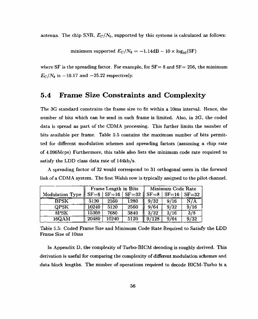
5.4 Frame Size Constraints and Complexity
The 3G standard constrains the frame size to fit within a IOms interval. Hence, the
number of bits which can be send in each frame is limited. -41~0, in 3G, the coded
data is spread as part of the CDMA processing. This further limits the number of
bits available per frame. Table 5.5 contains the maximum number of bits permit-
ted for different modulation schemes and spreading factors (assuming a chip rate
of 4.096EvIcps) Furthermore, this table also lists the minimum code rate required to
satisfy the LDD class data rate of 144kb/s.
A spreading factor of 32 would correspond to 31 orthogonal users in the forward
link of a CDMA system. The first Walsh row is typically assigned to the pilot channel.
Table 5.5: Coded Frame Size and Minimum Code Rate Required to Satisfy the LDD Frame Size of lOms
Modulation Type BPSK QPSK 8PSK
16QAM
In Appendiu D, the complexity of Turbo-BICM decoding is roughly derived. This
derivation is useful for comparing the complexity of different modulation schemes and
data block lengths. The number of operations required to decode BICM-Turbo is a
Frame Length in Bits SF=8 5120 10240 15360 20480
Minimum Code Rate SF=8 9/32 9/64 3/32 9/128
SF=16 2560 5120
' 7680 10240
SF=32 1280 2560 3840 5120
SF=16 9/16 9/32 3/16 9/64
SF=32 ' N/A
9/16
3/8 9/32 -
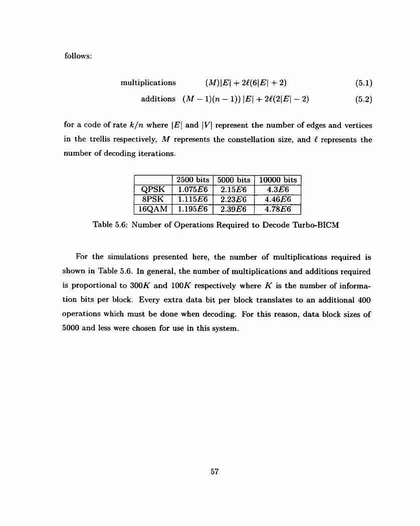
follows:
additions (M - l)(n - 1)) IEl +2[(21EI - 2 ) (5.2)
for a code of rate k/n where IEl and IV1 represent the number of edges and vertices
in the trellis respectively, M represents the constellation size, and e represents the
number of decoding iterations.
1 1 2500 bits 1 %00-bi& r i 0 0 0 0 bits 1 1 1 1 QPSK 1 1.075E6 1 2.15E6 1
1
4.366 1
Table 5.6: Number of Operations Required to Decode Turbo-BICM
For the simulations presented here, the number of multiplications required is
shown in Table 5.6. In general, the number of multiplications and additions required
is proportional to 300K and lOOK respectively where K is the number of informa-
tion bits per block. Every extra data bit per block translates to an additional 400
operations which must be done when decoding. For this reason, data block sizes of
5000 and less were chosen for use in this system.
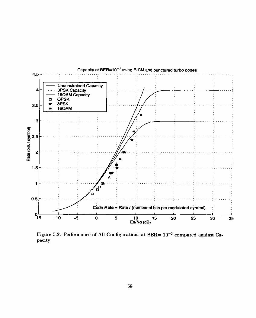
I 1 1 I I I I 1 1 I -1 5 -1 O -5 O 5 10 15 20 25 30 35
EdNo (dB)
Figure 5.2: Performance of Al1 Configurations at BER= 10-~ compared against Ca- pacity
Chapter 6
Conclusions
The performance of bit-interleaving versus symbol-interleaving in conjunction with
coded modulation has been evaluated over a variety of channels, as shown in Ta-
ble 6.1. While the performance of BICM and SICM had been previously examined
over AWGN and IID Rayleigh environments, we evaluated the two using more realistic
channels. We showed that over a one-path Doppler fading environment, BICM out-
performs SICM. We also showed that for short block lengths (2500 bits), IID Rayleigh
propagation is a valid assumption for estimating performance in a fast fading environ-
ment when either bit or symbol-interleaving is used. In 3G environments the winner
is not as clear for short block lengths. Our results suggest that as the number of
resolvable paths increases, the channel will look more and more Gaussian-like pro-
vided that R4KE reception is employed and that perfect channel state information is
available. In our comparison, 3-finger diversity reception is the threshold - less that
3-fingers, BICM outperforms SICM; greater that 3-fingers, SICM is better. While the
multipath provides diversity and mitigates fading, we have also shown that the ISI
induces an error floor a t high SNR - particularly noticeable for IGQAM. Since BICM
was shown to be 2M times more complex than SICM (where M is the constellation
size) it is recornmended that it be used in 3G environments only when the number of
RAKE fingers (and resolvable paths) is low.
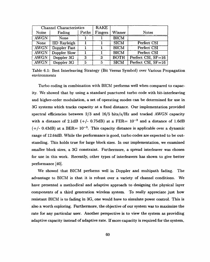
1 Channel Characteristics 1 R4KE 1
Table 6.1 : Best Interleaving Strategy (Bit Versus Symbol) over Various Propagation environments
Turbo coding in combination with BICM performs well when compared to capac-
ity. \Ve showed that by using a standard punctured turbo code with bit-interleaving
and higher-order modulation, a set of operating modes can be determined for use in
3G systems whicli tracks capacity a t a fixed distance. Our implementation provided
spectral efficiencies between 213 and 1615 bits/s/Hz and tracked AWGN capacity
with a distance of 2.ldB (+/- 0.75dB) at a FER= IO-* and a distance of 1.6dB
(+/- 0.43dB) a t a BER= This capacity distance is applicable over a dynamic
range of 12.64dB. While the performance is good, turbo codes are expected to be out-
standing. This holds true for large block sizes. In our implementation, we examined
smaller block sizes, a 3G constraint. Furthermore, a spread interleaver was chosen
for use in this work. Recently, other types of interleavers has shown to give better
Fingers 1 1 1 1 3 5
Paths 1 1 1 1 3 5
Soise AWGN None
AWGN AWGN AWGN -4WGN
performance [40].
We showed that BICM performs well in Doppler and multipath fading. The
advantage to BICM is that it is robust over a variety of channel conditions. We
have presented a methodical and adaptive approach to designing the physical layer
components of a third generation wireless system. To really appreciate just how
resistant BICM is to fading in 3G, one would have to simulate power control. This is
also a worth exploring. Furthermore, the objective of our system was to maximize the
Fading None
IID Rayleigh Doppler Fast Doppler Slow Doppler 3G Doppler 3G
rate for any particular user. Another perspective is to view the system as providing
adaptive capacity instead of adaptive rate. If more capacity is required for the system,
Winner BICM SICM BICM BICM BOTH SICM
Notes
Perfect CS1 Perfect CS1 Perfect CS1
Perfect CSI, SF=16 Perfect CSI, SF=16

lower the data rate of al1 users. This allows the base station to reduce the transmit
power required for each user and thereby increase system capacity. Although we have
covered many aspects of the system design, there are more areas yet to be covered.
We have, hoivever, provided a good starting point for future work.
Appendix A
BICM Metric Derivation
In conventional BICM [14, 13, 41, 161, the demodulator produces a set of maximum-
likelihood bit-metrics. A derivation of these metrics is presented next and is a sum-
marized version of one presented in 1141.
The transition probability density function of the channel is defined as
where cN, cN', and û represent N-dimensional Euclidean space, Nt-dimensional Eu-
clidean space, and the channel state respectively. 0 is assumed to be independent of
the x and the channel is assumed to be memoryless, so that
where the sequences { O ) = (O1,. . . , O*) , {x) = (xl,. . . , xk), and {y) = (yl,. . . , yi) and k is the sequence length. The likelihood function for y is
where @(x) denotes the ith bit of the label of x and SP is the subset of the signals
x E S whose label has the value b E {O, 1) in position 2 .
Next , a uniform(equiprobab1e) input distribut ion is assumed.
where A4 represents the number of points in the signal constellation. The log likeli-
hood function is then obtained
Finally, the constant term is removed from the equation and the BICM ML bit metric
at time t is defined.
where p represents the fading amplitude. It takes on a value of one for AWGN
channels.
Because this metric may be too computationally cornplex for implementation,
a log-sum approximation (log C j zj E maxj logzj) is often used. This sub-optimal
approximation is appropriate as long as the sum in the left-hand side of the equation
is dominated by a single term. The approximation is a good estimate at high signal-
to-noise ratios (SNR) [13]. The sub-optimal BICM bit-metric is
Appendix B
Turbo Codes
First discovered by Berrou et al. [42], turbo coding is a strategy by which two con-
stituent codes are concatenated together in a parallel fashion - separated by an inter-
leaver. An example of turbo encoder is presented in Figure B.1. The 16-state turbo
encoder has two constituent recursive, systematic, convolutional codes - each with
octal generators 37,21. This standard code has been shown to perform well in an
AWGN environment [43] and is the one chosen for use in this work.
Turbo codes have been shown to perform within a dB of capacity [42] for large
block sizes. The key ingredient for this remarkable performance lies in the iterative
decoding strategy used.
In decoding of turbo codes, each constituent is soft decoded using input information
which is the decoded information from the other code, as shown in Figure.
The decoding of each code is performed using the BCJR (or Forward/Backward
Algorithm) [44]. A set of calculated messages are passed in both the forward and
reversed directions of the trellis. At each depth of the trellis, a message (Ai for forward
and Bj for reverse) is calculated based on the message a t the previous depth(Ai- and
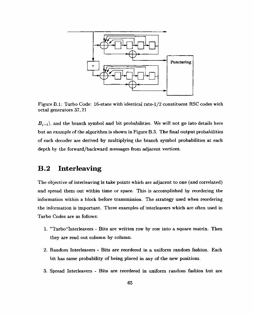
Figure B.l: Turbo Code: 16-state with identical rate-l/2 constituent RSC codes with octal generators 37,21
BjdI), and the branch symbol and bit probabilities. We will not go into details here
but an example of the algorithm is shown in Figure B.3. The final output probabilities
of each decoder are derived by multiplying the branch symbol probabilities at each
depth by the forward/backward messages from adjacent vertices.
B .2 Interleaving
The objective of interleaving is take points which are adjacent to one (and correlated)
and spread them out within time or space. This is accomplished by reordering the
information within a block before transmission. The strategy used when reordering
the information is important. Three examples of interleavers which are often used in
Turbo Codes are as follows:
1. "Turbo"Inter1eavers - Bits are written row by row into a square matrix. Then
they are read out coIumn by column.
2. Random Interleavers - Bits are reordered in a uniform random fashion. Each
bit has same probability of being placed in any of the new positions.
3. Spread Interleavers - Bits are reordered in uniform random fashion but are
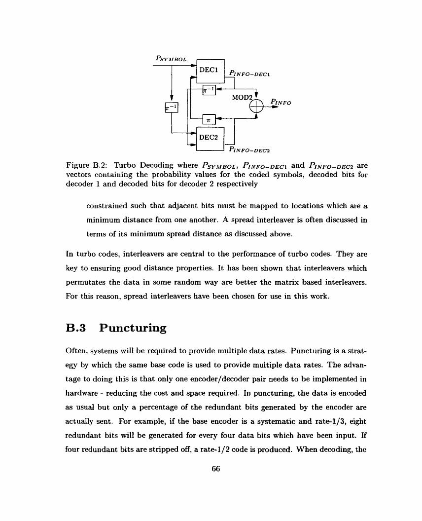
Figure B.2: Turbo Decoding where PSYMBOL, P I ~ ~ ~ - ~ E ~ ~ and PINFO-DEC~ are vectors containing the probability values for the coded symbols, decoded bits for decoder 1 and decoded bits for decoder 2 respectively
constrained such that adjacent bits must be mapped to locations which are a
minimum distance from one another. A spread interleaver is often discussed in
terms of its minimum spread distance as discussed above.
In turbo codes, interleavers are central to the performance of turbo codes. They are
key to ensuring good distance properties. It has been shown that interleavers which
permutates the data in some random way are better the matrix based interieavers.
For this reason, spread interleavers have been chosen for use in this work.
B.3 Puncturing
Often, systems will be required to provide multiple data rates. Puncturing is a strat-
egy by which the same base code is used to provide multiple data rates. The advan-
tage to doing this is that only one encoder/decoder pair needs to be implemented in
hardware - reducing the cost and space required. In puncturing, the data is encoded
as usual but only a percentage of the redundant bits generated by the encoder are
actually sent. For example, if the base encoder is a systematic and rate-113, eight
redundant bits will be generated for every four data bits which have been input. If
four redundant bits are stripped off, a rate-1/2 code is produced. When decoding, the
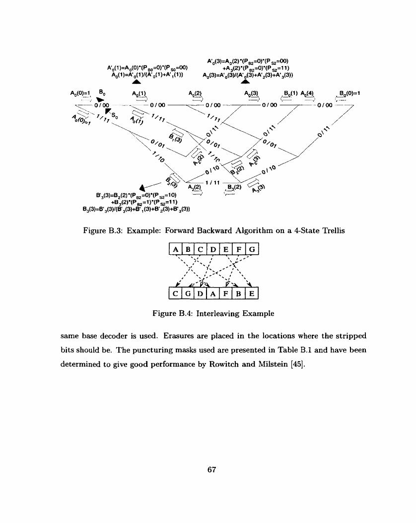
Figure B.3: Example: Forward Backward Algorithm on a 4-State Trellis
Figure B.4: Interleaving Example
same base decoder is used. Erasures are placed in the locations where the stripped
bits shoulci be. The puncturing masks used are presented in Table B.1 and have been
determined to give good performance by Rowitch and Milstein [45].
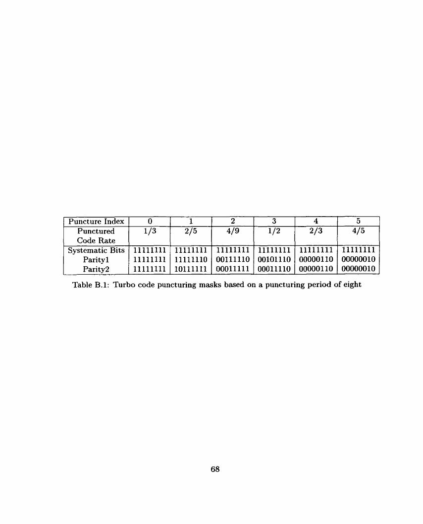
Table B.1: Turbo code puncturing masks based on a puncturing period of eight
Puncture Index Punctured Code Rate
Systematic Bits Pari ty 1 Paritv2
O 1/3
11111111 11111111 11111111
1 215
11111111 11111110 10111111
2 4/9
11111111 00111110 O0011111
3 112
11111111 00101110 00011110
4
2/3
l l l l l l l l O0000110 00000110
5 4/5
11111111 00000010 00000010
Appendix C
Bit-Error-Rate (BER) Curves
The simulation results for the 16-state turbo code are illustrated in the figures pre-
sented in this section.
This code is punctured to achieve code rates of 1/3, 2/5, 4/9, 1/2, 2/3, and 4/5.
The coded outputs are modulated using QPSK, 8PSK, or IGQAM. Organized by
rate, each figure contains a plot of BER versus Eb/N,, for each of QPSK, 8PSK and
16QAM. In most cases, the results are presented for information block lengths of 1000
and 5000. Also the bit SNR required to achieve capacity for each of the modulation
types is highlighted via a line on the plot (the leftmost line is QPSK, followed by
8PSK and then 16QAM). The equation used to calculate the SNR which achieves
capacity (see [32]) is as follows:
where Eb, Es, and & are the average bit energy, average symbol energy and the
noise power spectral density respectively. The channe1 coding rate, R, is defined as
the punctured turbo code rate times the spectral efficiency of the modulation used.
For example, if the code rate is 213 and the modulation is 8PSK, the channel coding
rate is 2 bits/symbol/2D.
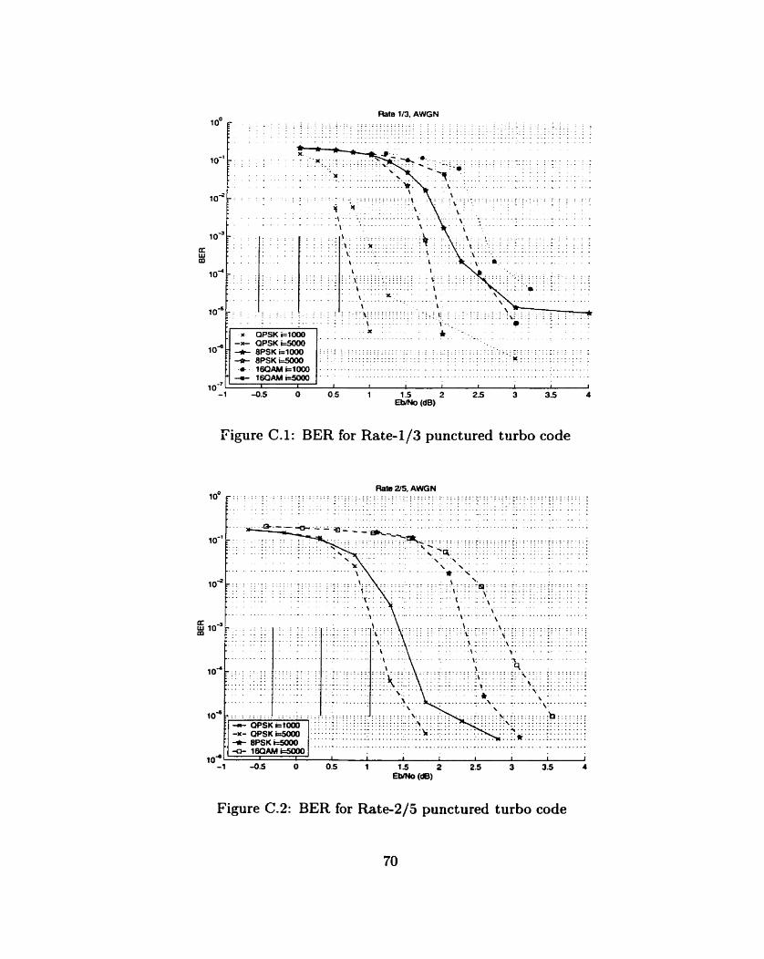
Rate 113, AWGN 1 o0
l . \ - k
% : - \ \
104 1
10" -
x OPSK ~ 1 0 0 0 -x- QPSK t5000
104 E + BPSK el000 : + â P S K i 5 0 W
* 16QAMd000 -a- 16aAMr=5000
IO-' .
I 1 1 I I I I 1 I
-1 -0.5 O 05 1 1.5 2 2 5 3 35 4 E m (dB)
Figure C.l : BER for Rate-113 punctured turbo code
Rals 215. AWGN
Figure C.2: BER for Rate-2/5 punctured turbo code
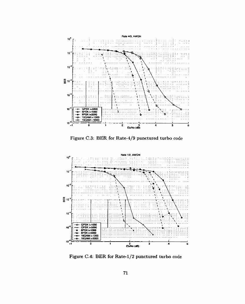
Rate a. AWGN
1041 ' 1 1 1 1 1 I
-1 O 1 2 3 4 5 6 EWNo (dB)
Figure (2.3: BER for Rate-4/9 punctured turbo code
Figure C.4: BER for Rate-1/2 punctured turbo code
71

Rate 213. AWGN 10"
f
Figure C.5: BER for Rate-213 punctured turbo code
IO-'
Rôîû US. AWGN I " ~ : . . . . . . . . . . . . . . . . . . . . . . . . . . . . . . . . . . . . . . . . . . . . . . . . . . . . . . . . . . . . . . . . . . . . . . . . . . . . . . . . . . . . . . - . . . . . . - . . . . . . . - . - . -. . . . . . . . . . . . . . . . . . . . . . . . . . . . . . . . . . . . . . . . . . . . . . . . . . . . . . . . . . . . . . . . . . . . . . . . . . . . . . . . . . . . . . . . . . . . . . . . . . . . . . . . . . . . . . . . . . . . . . . . . . . . . . . . . . . . . . . . . . . . . . . . . . . . . . . . . . . . . . . . . . . . . . . . . . . . . . . . . . . . . . . . - - .
. . . . . . . . . . . . . . . . . . . . . . . . . . . . . . . . . . . . . . . . . . . . . . . . . . . . . . . . . . . . . . . . . . . . .
10-~
2 loar
104
10"
1 o4 -4
-DI- QPSK t t W û
+ 16oMAt5000 104
-3 -2 -1
.......................................... . . . . . . ................................................
. . . . . . . . . . .- ................................................... - . ........ -. 1 I 1 1 1 1 1 1
O 1 2 3 4 5 6 7 E m (dB)
EWNo (dB)
7
-
Figure C.6: BER for Rate-415 punctured turbo code
y : - . -
- QPSK ~ 1 0 0 0 -x- QPSK t=5000 + 8PSKi=1000
-û- BPSKk5000 * lBQAMt=looO : -F 1 w A M r=5000
I I 1 I 1 1 1 1 1
-3 -2 -1 O 1 2 3 4 5 6
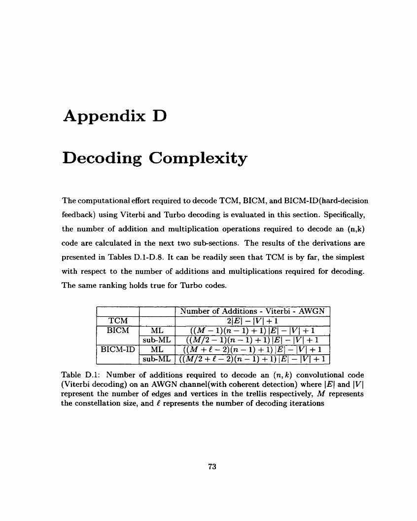
Appendix D
Decoding Complexity
The computational eifort required to decode TCM, BICM, and BICM-ID(hard-decision
feedback) using Viterbi and Turbo decoding is evaluated in this section. Specifically,
the number of addition and multiplication operations required to decode an (n, k)
code are calculated in the next two sub-sections. The results of the derivations are
presented in Tables D. 1-D.8. It can be readily seen t hat TCM is by far, the simplest
with respect to the number of additions and multiplications required for decoding.
The same ranking holds true for Turbo codes.
1 1 Number of Additions - Viterbi - AWGN
Table D.1: Number of additions required to decode an (n, k) convolutional code (Viterbi decoding) on an AWGN channel(with coherent detection) where IEl and 1 VI represent the number of edges and vertices in the trellis respectively, M represents the constellation size, and Q represents the number of decoding iterations
. . . .
( ( M - l ) (n - 1) + 1) lEl - IV1 + 1 ( ( M / 2 - l ) ( n - l ) + l ) I E l - I V I + l
( ( M + Q - 2 ) ( n - l ) + l ) I E I - I v I + l ( ( M / 2 + k' - 2)(n - 1) + 1) [El - IV1 + 1
BIChd
BICM-ID
ML sub-ML
ML sub-ML

1 Number of Multi~lications - Viterbi - AWGN 1
BICM-ID ML SU^-ML ( ~ ç 1 / 2 + e ) 1 E 1
Table D.2: Number of multiplications required to decode an (n, k) convolutional code (Viterbi decoding) on an AWGN channel(with coherent detection) where IEl and IV1 represent the number of edges and vertices in the trellis respectively, fil represents the constellation size, and e represents the number of decoding iterations
Table D.3: Number of additions required to decode an (n, k) convolutional code (Viterbi decoding) on a Rayleigh channel(with perfect CSI) where IEl and IV1 r e p resent the number of edges and vertices in the trellis respectively, M represents the constellation size, and e represents the number of decoding iterations
TCM BICM
BICM-ID
D.l Viterbi Decoding
Decoding of the BICM system using convolutional codes is generally done using the
Viterbi [46] algorithm. The number of operations required to irnplement the Viterbi
algorithm is well documented and a derivation is presented in McEliece [44]. Specifi-
cally, the number of addition and multiplication operations for a given Viterbi decoded
code C are:
ML sub-ML
ML sub-ML
multzplicatias = IEl
additions = IEl - IV1 + 1
Nurnber of Additions - Viterbi - Rayleigh 21EI - IV1 + 1
((M - l ) ( n - 1) +1) IEl- IV1 +1 ( ( M / 2 - l)(n - 1) + 1) lEl- IV1 + 1 ((M + e - 2)(n - 1) + 1) IEI - JVI + 1
( ( M / 2 + e - z ) ( n - l ) + l ) I E I - I V I + l
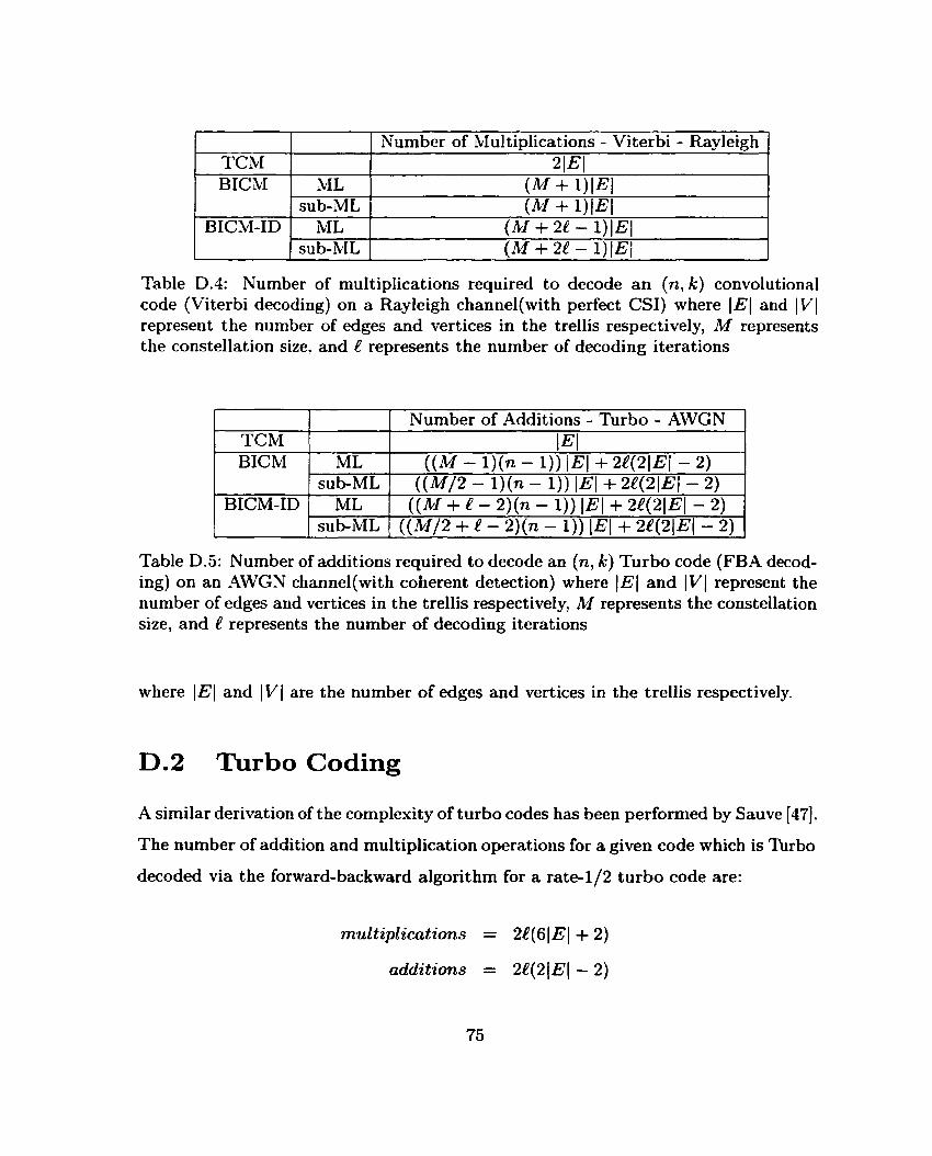
- - -- -- - - --
Table D.4: Number of multiplications required to decode an (n, k) convolutional code (Viterbi decoding) on a Rayleigh channel(with perfect CSI) where IEl and IV1 represent the number of edges and vertices in the trellis respectively, M represents the constellation size, and e represents the number of decoding iterations
TCM
r 1 1 Number of Additions - Turbo - AWGN 1
Number of Multiplications - Viterbi - Rayleigh 21El
Table D.5: Number of additions required to decode an (n, k) Turbo code (FBA decod- ing) on an AWGN channel(with coherent detection) where IEl and IV1 represent the number of edges and vertices in the trellis respectively, M represents the constellation size, and t represents the nurnber of decoding iterations
TCM BICM
BICM-ID
where IEl and IV1 are the number of edges and vertices in the trellis respectively.
D.2 Turbo Coding
ML sub-ML
ML sub-ML
A similar derivation of the complexity of turbo codes has been performed by Sauve [47].
The number of addition and multiplication operations for a given code which is Turbo
decoded via the forward-backward algorithm for a rate412 turbo code are:
!El ((M - l ) ( n - 1)) /El + 2[(21EI - 2)
( ( M / 2 - l)(n - 1)) JE1 + 2.f(21El - 2) '
( (W + e - 2)(n- 1)) IEl +2[(21EI - 2) ( ( M / 2 + t - 2 ) ( n - l ) ) I E l + 2 e ( 2 l E I - 2 )
multiplications = Z ( 6 ) E 1 + 2)
additions = 2t(21E( - 2)
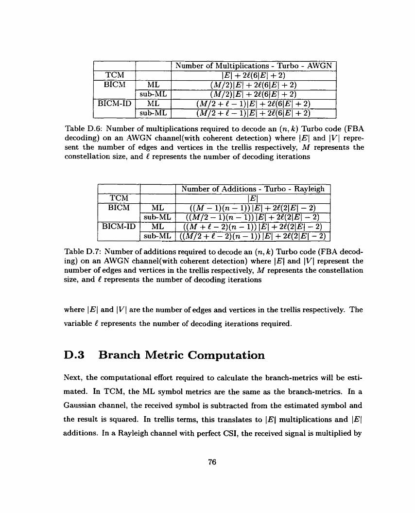
1 1 1 Number of Multiplications - Turbo - AWGN (
Table D.6: Nurnber of multiplications required to decode an (n, k) Turbo code (FBA decoding) on an AWGN channel(with coherent detection) where IEl and IV1 repre- sent the number of edges and vertices in the trellis respectively, M represents the constellation size, and l represents the number of decoding iterations
TCM
Table D.7: Number of additions required to decode an (n, k) Turbo code (FBA decod- ing) on an AWGN channel(with coherent detection) where IEl and IV1 represent the number of edges and vertices in the trellis respectively, M represents the constellation size, and represents the number of decoding iterations
Number of Additions - Turbo - Rayleigh IEI
L
BICM
BICM-ID
where 1 E 1 and 1 V 1 are the number of edges and vertices in the trellis respectively. The
variable t? represents the number of decoding iterations required.
D.3 Branch Metric Computation
ML sub-ML
ML sub-ML
Next, the computational effort required to calculate the branch-metrics will be esti-
mated. In TCM, the ML symbol metrics are the same as the branch-metrics. In a
Gaussian channel, the received symbol is subtracted from the estimated symbol and
the result is squared. In trellis terms, this translates to IE( multiplications and IEl
additions. In a Rayleigh channel with perfect CSI, the received signal is multiplied by
((Al - l)(n - 1)) [El + 2[(21EI - 2) ((M/2 - l ) (n - 1)) 1 El + 2l(21 E 1 - 2)
((M + e - 2)(n - 1)) IEl +2e(21EI - 2) ((M/2 + e - 2)(n - 1)) IEl + 2l(21El - 2)
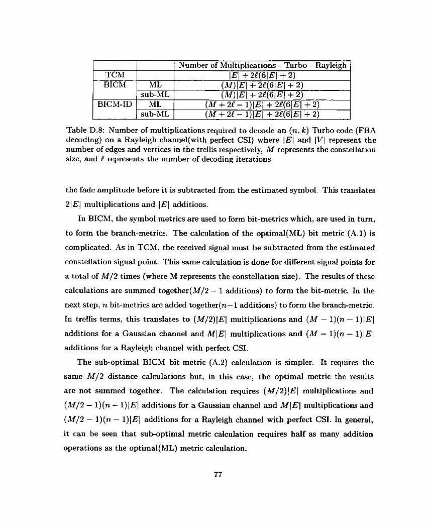
Table D.8: Number of multiplications required to decode an (n, k) Turbo code (FBA decoding) on a Rayleigh channel(with perfect CSI) where JE1 and IVJ represent the number of edges and vertices in the trellis respectively, M represents the constellation size, and k' represents the number of decoding iterations
TC k1 BICM
BICM-ID
the fade amplitude before it is subtracted from the estimated symbol. This translates
2 1 El multiplications and 1 E 1 additions.
In BICM, the symbol metrics are used to form bit-metrics which, are used in turn,
to form the branch-metrics. The calculation of the optimal(ML) bit metric (A.1) is
complicated. -4s in TCM, the received signal must be subtracted from the estimated
constellation signal point. This same calculation is done for different signal points for
a total of M / 2 times (where M represents the constellation size). The results of these
calculations are summed together(Ml2 - 1 additions) to form the bit-metric. In the
next step, n bit-metrics are added together(n- 1 additions) to form the branch-metric.
In trellis terms, this translates to (M/2)IEI multiplications and (M - l ) ( n - 1)IEl
additions for a Gaussian channel and MIE1 multiplications and ( M - l)(n - 1)IEl
additions for a Rayleigh channel with perfect CSI.
The sub-opt imal BICM bit-metric (A.2) calculation is simpler. It requires the
same M / 2 distance calculations but, in this case, the optimal metric the results
are not summed together. The calculation requires ( M / 2 ) 1 E 1 multiplications and
( M / 2 - 1) (n - 1) 1 E 1 additions for a Gaussian channel and M 1 E 1 multiplications and
( M / 2 - 1) (n - 1) IEl additions for a Rayleigh channel with perfect CSI. In general,
it can be seen that sub-optimal metric calculation requires half as many addition
operations as the optimal(ML) metric calculation.
ML sub-ML
ML sub-ML
Number of Multiplications - Turbo - Rayleigh IEI + 2e(61EI + 2)
(M)IEl + Ze(61EJ + 2) - (M)IEI + Pe(6 lEl t 2)
( M + 2C - 1)IEl + 2e(61EI + 2) ( M + 2t - 1)IEl + 2e(61EI + 2)
BICM-ID requires the same number of operations as BICM for first pass decoding.
On subsequent decoding cycles, calculation of the bit-metric is less complex. The de-
coder feeds back an estimated signal constellation point. Far this reason the distance
calculation needs is performed only once on the e - 1 subsequent decoding cycles([
represents the total number of iterations) . In total, the optimal bit-metric calculation
requires ((iC1/2) + l - 1) 1 E 1 multiplications and ( M + l - 2) (n - 1) (El additions for
a Gaussian channel and (hl + 2 - 2)IEI multiplications and ( M + e - 2)(n - 1)IEl
additions for a Rayleigh channel with perfect CSI.
Sub-optimal BICM-ID metric calculation is similar. The sub-optimal bit-metric
calculation requires ((M/2) + k' - 1) 1 El multiplications and ( M l 2 + P - 2 ) ( n - 1 ) 1 E 1 additions for a Gaussian channel and (M + 2e - 2))EI multiplications and ( M / 2 + e - 2) ( n - 1 ) 1 E 1 additions for a Rayleigh channel with perfect CSI.

Bibliography
[l] Dataquest Inc., "Gartner dataquest predicts half a billion mobile phones should
be sold during 2001 ," Tech. Rep., March 2001, http://wwwS.gartner.corn.
[2] V. H. MacDonald, "The cellular concept," Bell System Technical Journal, vol.
38 (l) , pp. 15-41, 1979.
[3] E. Sousa, "CDMA mobile radio communications, - ece1543," Edward S. Rogers
Sr. Department of Electrical and Computer Engineering, University of Toronto,
Mar. 2001.
[4] R. C. Dixon, Spread Spectrum Systems, Wiley, New York NY, 1st edition, 1984.
[5] D. L. Schilling, R. L. Pickholtz, and L. M. Milstein, "Spread spectrum goes
commercial," IEEE Spectrrrm, pp. 40-45, Aug . 1990.
[6] G. R. Cooper and R. W. Nettleton, "A spread-spectrum technique for high
capacity mobile communications," IEEE Trans. on Veh. Tech., vol. VT-7(4),
pp. 39-40, Nov. 1978.
[7] E. Sousa, "Class notes for mobile communications - ECE1543," Edward S.
Rogers Sr. Department of Electrical and Computer Engineering,University of
Toronto, Mar. 2001.
[8] IMT2000, "The road to IMT2000," Tech. Rep., 2001, http://www.itu.int/imt.
[9] R. Price and P. E. Green, "-4 communication technique for multipath cliannels,"
Proc. IRE, vol. 46, pp. 555-570, March 1958.
[IO] G. Ungerboeck, "Channel coding with multilevel/phase signals," IEEE Trans.
Inform. Theory, vol. IT-28, pp. 55-67, May 1982.
[11] H. Imai and S. Hirakawa, "A new multilevel coding method using error correcting
codes," IEEE Trans. Inform. Theory, vol. IT-23, pp. 371-377, May 1977.
[12] C.-E. Sundberg and N. Seshadri, "Coded modulations for fading channels: An
overview," Europ. Trans. Telecornm. (ETT), pp. 309-324, May-June 1993.
[13] E. Zehavi, "8-PSK trellis codes for a Rayleigh channel," IEEE Trans. Commun.,
vol. 40, pp. 873-884, 1992.
[14] G. Caire, G. Taricco, , and E. Biglieri, "Bit-interleaved coded modulation,"
IEEE Trans. Inform. Theory, vol. 44, pp. 927-946, May 1998.
[15] U. Wachsmann, J. Huber, and P. Schramm, "Serial concatenation of interleaved
codes: Performance and analysis, design, and iterative decoding," Proc. IEEE
Int. Syrnp. Infonn. Theory (ISIT), p. 5, Aug. 1998.
[16] X. Li and J. A. Ritcey, "Trellis-coded modulation with bit interleaving and
iterative decoding," IEEE J. Select. Areas Commun., vol. 17(4), pp. 715-724,
Apr. 1999.
[17] X. Li and J. A. Ritcey, LLBit-interleaved coded modulation with iterative decoding
using soft feedback," Electronic Letters, vol. 34(10), pp. 942-943, May 1998.
[18] T. S. Rappaport, W2reless Communications: Principles and Practices, Prentice
Hall, Englewood Cliffs NJ, 1996.
[19] S. Jamali and T. Le-Ngoc, Coded-modulation techniques for fading channels,
Kluwer, New York NY, 1994.
[20] J. G. Proakis, Digital Communications, McGraw-Hill, New York NY, 3rd edition,
1996.
[21] R. H. Clarke, "A statistical theory of mobile-radio reception," Bell System
Technical Journal, vol. 47, pp. 957-1000, 1968.
[22] M. J. Gans, "A power spectral theory of propagation in the mobile radio envi-
ronment," IEEE Trans. on Veh. Tech., vol. VT-21, pp. 27-38, Rb. 1972.
[23] J. 1. Smith, "A computed generated multipath fading simulation for mobile
radio," IEEE Trans. on Veh. Tech., vol. VT-24(3), pp. 39-40, Aug. 1975.
[24] H. Mahvidi, "Performance of latency constrained turbo-like codes over correlated
fading channels," M.A.Sc. thesis, University of Toronto, Toronto ON, 2000.
[25] J. G. Proakis and D. G. Manolakis, Digital Signal Processing, Prentice-Hall,
Upper Saddle River NJ, 3rd edition, 1996.
[26] X. Li and 5. .A. Ritcey, "Bit-interleaved coded modulation with iterative decod-
ing," IEEE Int. Conf. Communication, vol. 2, pp. 858-863, May 1999.
[27] S. Benedetto, D. Divsalar, G. Montorsi, and F. Pollara, "A soft-input soft-output
A P P module for iterative decoding of concatenated codes," IEEE Commun.
Letters, vol. 1, pp. 22-24, Jan. 1997.
[28] S. Lin and D. J. Costello Jr., Error Contml Coding: Fundarnentals and Appli-
cations, Prentice-Hall, Englewood Cliffs NJ, 1983.
[29] R. J. Mantha, "Hybrid automatic repeat request schemes using turbo codes and
low density parity check codes," M. ASC. thesis, University of Toronto, Toronto
ON, 1999.
[30] S. Benedetto, M. Mondin, and G. Montorsi, "Performance evaluation of trellis-
coded modulation schemes," Proc. IEEE, vol. 82(6), June 1994.

[31] F. Kschischang, "Class notes for error control codes - ECE1501," Esdward S.
Rogers Sr. Department of Electical and Computer Engineering, University of
Toronto, Oct. 1999.
[32] S. Cover and J. Thomas, Elements of Information Theoqj, Wiley, New York
NY, 1991.
[33] G. Taricco G. Caire and E. Biglieri, "Capacity of bit-interleaved channels,"
Electronic Letters, vol. 32, pp. 1060-1061, June 1996.
[34] B. Melis and G. Romano, "UMTS W-CDMA: Evaluation of radio performance
by means of link level simulations," IEEE Pers. Commun., pp. 42-49, June 2000.
[35] 3GPP, "Selection procedures for the choice of radio transmission technologies of
the UMTS," TS UMTS 30.03 version 3.1.0, Nov. 1997.
[36] D. Brennan, "Linear diversity cornbining techniques," Proc. IRE, vol. 47, pp.
1075-1102, June 1959.
[37] M. S Alouini, S. Kim, and A. Goldsmith, "Rake reception with maximum-ratio
and equal-gain combining for DS-CDMA systems in Nakagarni fading," IEEE
Int. Conf. Uniu. and Pers. Comm., vol. 2, pp. 708-712, 1997.
[38] S. B. Wicker, Error Control Systems for Digital Communication and Storage,
Prentice Hall, Englewood Cliffs NJ, 1995.
[39] S. Kallel, "Efficient hybrid AR& protocols with adaptive forward error correc-
tion," IEEE Trans. Commun., pp. 291-289, Feb. 1994.
[40] S. N. Crozier, "New high-spread high-distance interleavers for turbo codes,"
Proc. Bienn. Symp. Info. Theory, pp. 3-7, May 2000.
[41] X. Li and J. A. Ritcey, "Bit-interleaved coded modulation with iterative decod-
ing," IEEE Commun. Lett., vol. 1, pp. 169-171, Nov. 1997.

[42] C. Berrou, -4. Glavieux, and P. Thitimajshima, "Near Shannon limit error-
correcting coding and decoding: Turbo codes," IEEE Int. Conf. Communication,
pp. 1064-2070, May 1993.
[43] S. Benedetto, D. Divsalar, G. Mont orsi, and F. Pollara, "Serial concatenation
of interleaved codes: Performance and analysis, design, and iterative decoding,"
IEEE Trans. Inform. Theory, vol. 44, pp. 909-926, May 1988.
[44] R. J. McEliece, "On the BCJR trellis for linear block codes," IEEE Trans.
Infonn. Theory, vol. 42(4), pp. 1072-1092, July 1996.
[43] D. N. Rowitch and L. B. Milstein, "On the performance of hybrid FEC/ARQ
systems using rate compatible punctured turbo (RCPT) codes," IEEE Trans.
Commun., vol. 48(6), pp. 948-959, June 2000.
[46] A. Viterbi, "Error bounds for convolut ional codes and as asymptotically optimum
decoding algorithm," IEEE Trans. Inform. Theory, vol. IT-13, pp. 260-269, Apr.
1967.
[47] P.-P. Sauve, "Multibit turbo decoding of turbo codes," M.A.Sc. thesis, University
of Toronto, Toronto ON, 1998.
[48] R. J. McEliece, L'The trellis complexity of convolutional codes," IEEE Trans.
Inform. Theory, vol. 42(4), pp. 1855-1864, Nov. 1996.
[49] J. Wozencraft and B. Reiffen, Sequential Decoding, MIT Press, Cambridge MA,
3rd edition, 1961.
[50] G . Forney, Concatenated Codes, MIT Press, Cambridge MA, 1966.