ADABOOST GPU-BASED CLASSIFIER FOR DIRECT VOLUMERENDERING

Oscar Amoros1, Sergio Escalera2, and Anna Puig3

1Barcelona Supercomputing Center - CNS, K2M Building, c/ Jordi Girona, 29 08034 Barcelona, Spain2UB-Computer Vision Center, Campus UAB, Edifici O, 08193, Bellaterra, Barcelona, Spain

3WAI-MOBIBIO Research Groups, University of Barcelona, Avda.Corts Catalanes, 585, 08007 Barcelona, Spainoamorohu7@alumnes.ub.edu, {sergio,anna}maia.ub.es

Keywords: Volume Rendering, High-Performance Computing and Parallel Rendering, Rendering Hardware

Abstract: In volume visualization, the voxel visibitity and materials are carried out through an interactive editing ofTransfer Function. In this paper, we present a two-level GPU-based labeling method that computes in timesof rendering a set of labeled structures using the Adaboost machine learning classifier. In a pre-processingstep, Adaboost trains a binary classifier from a pre-labeled dataset and, in each sample, takes into account aset of features. This binary classifier is a weighted combination of weak classifiers, which can be expressed assimple decision functions estimated on a single feature values. Then, at the testing stage, each weak classifieris independently applied on the features of a set of unlabeled samples. We propose an alternative represen-tation of these classifiers that allow a GPU-based parallelizated testing stage embedded into the visualizationpipeline. The empirical results confirm the OpenCL-based classification of biomedical datasets as a toughproblem where an opportunity for further research emerges.

1 INTRODUCTION

The definition of the visibility and the optical proper-ties at each volume sample is a tough and non intuitiveuser guided process. It is often performed throughthe user definition of Transfer Functions (TF). Selec-tion of regions is defined indirectly by assigning tozero the opacity since totally transparent samples donot contribute to the final image. The use of TFs al-lows to store them as look-up tables (LUT), directlyindexed by the intensity data values during the vi-sualization, which significantly speeds up renderingand it is easy to implement in GPUs. In previousworks, the transfer function is broken into two sepa-rated steps (Cerquides et al., 2006): the ClassificationFunction (CF) and the optical properties assignment.The Classification Function determines at each pointinside the voxel model at which specific structure thepoint belongs. Next, the optical properties assignmentis a simple mapping that assigns to each structure aset of optical properties. In this approach, we focuson the definition and the improvement of the Classifi-cation Function and its integration into the renderingprocess. The main advantage of the classification ap-

proach is that, since a part of the classification can becarried on a pre-process, before rendering, it can usemore accurate and computationally expensive classi-fication methods than transfer functions mappings.

Specifically, we use a learning-based classifica-tion method that splits into two steps: learning andtesting. In the learning step, given a set of train-ing examples, each marked by an end-user as belong-ing to one of the set of the labels or categories, theAdaboost-based Machine Learning training algorithmbuilds a model, or classifier, that predicts whether anew voxel falls into one category or the other. In thetesting stage, the classifier is used to classify a newvoxel description. Thus, the learning step is done ina pre-process stage, though the testing step is inte-grated on-the-fly into the GPU-based rendering. Inthe rendering step, at each voxel value, the classifieris applied to obtain a label. We propose a GPGPUstrategy to apply the classifier, interpret the voxels asthe set of objects to classify, and their property values,derivatives and positions as the attributes or featuresto evaluate. We apply a well-known learning methodto a sub-sampled set of already classified voxels andnext we classify a set of voxel models in a GPU-based

testing step. Our goal is three-fold:• to define a voxel classification method based on a pow-

erful machine learning approach,

• to define a GPGPU-based testing stage of the proposedclassification method integrated to the final rendering,

• to analyze the performance of our method compar-ing five different implementations with different publicdata sets on different hardware.

2 ADABOOST CLASSIFIERIn this paper, we focus on the Discrete version of Ad-aboost, which has shown robust results in real ap-plications (Friedman et al., 1998). Given a set of Ntraining samples (x1,y1), ..,(xN ,yN), with xi a vectorvalued feature and yi = −1 or 1, we define F(x) =∑

M1 c f fm(x) where each fm(x) is a classifier produc-

ing values ±1 and cm are constants; the correspond-ing prediction is sign(F(x)). The Adaboost proceduretrains the classifiers fm(x) on weighted versions ofthe training sample, giving higher weights to casesthat are currently misclassified. This is done for a se-quence of weighted samples, and then the final clas-sifier is defined to be a linear combination of the clas-sifiers from each stage. For a good generalization ofF(x), each fm(x) is required to obtain a classificationprediction just better than random (Friedman et al.,1998). Thus, the most common ”weak classifier” fmis the ”decision stump”. Stumps are single-split treeswith only two terminal nodes. If the decision of thestump obtains a performance inferior to 0.5 over 1, wejust need to change the polarity of the stump, assur-ing a performance greater (or equal) to 0.5. Then, foreach fm(x) we just need to compute a threshold valueand a polarity to take a binary decision, selecting thatone that minimizes the error based on the assignedweights.

In Algorithm 1, we show the testing of the final de-cision function F(x) = ∑

M1 c f fm(x) using the Discrete

Adaboost algorithm with Decision Stump ”weak clas-sifier”. Each Decision Stump fm fits a threshold Tmand a polarity Pm over the selected m-th feature. Intesting time, xm corresponds to the value of the fea-ture selected by fm(x) on a test sample x. Note that cmvalue is subtracted from F(x) if the hypothesis fm(x)is not satisfied on the test sample. Otherwise, positivevalues of cm are accumulated. Finally decision on x isobtained by sign(F(x)).

1: Given a test sample x2: F(x) = 03: Repeat for m = 1,2, ..,M:

(a) F(x) = F(x)+ cm(Pm · xm < Pm ·Tm);4: Output sign(F(x))

Algorithm 1: Discrete Adaboost testing algorithm.

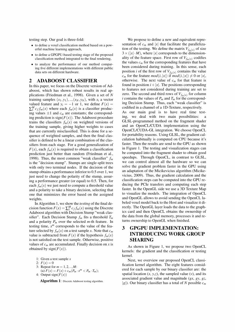
We propose to define a new and equivalent repre-sentation of cm and |x| that facilitate the paralleliza-tion of the testing. We define the matrix Vfm(x) of size3× (|x| ·M), where |x| corresponds to the dimension-ality of the feature space. First row of Vfm(x) codifiesthe values cm for the corresponding features that havebeen considered during training. In this sense, eachposition i of the first row of Vfm(x) contains the valuecm for the feature mod(i, |x|) if mod(i, |x|) 6= 0 or |x|,otherwise. The next value of cm for that feature isfound in position i+ |x|. The positions correspondingto features not considered during training are set tozero. The second and third rows of Vfm(x) for columni contains the values of Pm and Tm for the correspond-ing Decision Stump. Thus, each “weak classifier” iscodified in a channel of a 1D-Texture, respectively.As our main goal is to have real time test-ing, we deal with two main possibilities: aGLSL-programmed method on the fragment shaderand an OpenCL/CUDA implementation using theOpenCL/CUDA-GL integration. We choose OpenCLfor portability reasons. Using GLSL, the gradient cal-culation habitually is computed on CPU because it’sfaster. Then the results are send to the GPU as shownin Figure 1. The testing and visualization stages canbe computed into the fragment shader to obtain goodspeedups. Through OpenCL, in contrast to GLSL,we can control almost all the hardware so we cansolve the gradient problem faster in the GPU usingan adaptation of the Micikevicius algorithm (Micike-vicius, 2009). Thus, the gradient calculation and theclassification steps can be computed into the GPU re-ducing the PCIe transfers and computing each stepfaster. In the OpenGL side we use a 3D Texture Mapto visualize the models. The integration of OpenCLand OpenGL allows to avoid sending the OpenCL la-beled voxel model back to the Host and visualize it di-rectly. The OpenGL layer loads the data to the graph-ics card and then OpenCL obtains the ownership ofthe data from the global memory, processes it and re-turns ownership to OpenGL when finished.

3 GPGPU IMPLEMENTATION:INTRODUCING WORK GROUPSHARING

As shown in Figure 1, we propose two OpenCLkernels: the gradient and the classification or testingkernel.

Next, we overview our proposed OpenCL classi-fication kernel algorithm. The eight features consid-ered for each sample by our binary classifier are: thespatial location (x, y,z), the sampled value (v), and itsassociated gradient value and magnitude (gx, gy, gz,|g|). Our binary classifier has a total of N possible cm

Figure 1: GPGPU implementation overview: GLSL and OpenCL approaches.

values, with N = 3 ·M. We create a matrix of Work-Groups (WG) that covers the x and y dimensions ofthe dataset, whereas the component z is computed in aloop. Each WG classifies one voxel. Inside each WG,we define N · 8 threads or WorkItems (WI) where Nis a multiple of two. Each WI computes a single stepwith the three weights weak classifiers and producesa value. These N ·8 values will be reduced at the endof the execution. This process parallelizes the step3 of the Discrete Adaboost testing algorithm definedin Algorithm 1. Finally, the sign of this computedvalue (sign(F(x))) is used to obtain the label of theprocessed voxels.

The way we are using threads and Global Memorytransfers follows what we call Work Group Sharing(WGS), a short form of Work Group global memorytransfer sharing. Our WGS method is characterizedby:

• Counter intuitive global memory use. A work groupreads minimum global memory data and produces theresult for a single voxel. Classifying different voxels al-lows the work group to read at maximum global mem-ory bandwidth. It is as to say that several work groupsshare a single global memory transaction, but in fact weare using only one WG.

• To process n voxels we can use 240 threads serializingn steps instead of using n threads serializing 240 stepseach one. That gives a greater number of threads and soforth better performance (latency hiding) and scalabil-ity.

• Local memory gets alleviated. We store n half voxelsinstead of 240 for each workgroup.

In summary, finer grain parallelization, more localmemory and more registers available allow to extratune the code for faster execution.

4 SIMULATIONS AND RESULTSIn order to present the results, first, we define the

data, methods, hardware platform, and validation pro-tocol.

• Data: We used three datasets: the Thorax data set rep-resents a phantom human body; Foot and Hand are CTscan of a human foot and a human hand, respectively.

• Methods: We use a Discrete Adaboost classifier with30 Decision Stumps and codified the testing classifierin Matlab, C++, OpenMP, GSGL, and OpenCL codes.

• Hardware platform: We used a Pentium Dual Core 3.2GHz with 3GB of RAM and equipped with a NVIDIAGeforce 8800 GTX with 1 GB of memory running a64-bit Ubuntu Linux distribution, a PC with a quad corePhenom2 x4 955 processor with 4GB of DDR3 mem-ory equipped with an NVDIA Geforce GTX470 with1,28 GB of memory. The viewport size is 700×650.

• Validation protocol: We compute the mean executiontime from 500 code runs. For accuracy analysis, weperformed stratified ten-fold cross-validation.

The classification performance of the Adaboost-GPU classifier on each individual dataset is analyzedin Table 1. We defined different binary classificationproblems of different complexity for the three medi-cal volume datasets. Last column of the table showsthe number of weak classifiers required by the clas-sifier in order to achieve the corresponding perfor-mance. For the different binary problems we achieveperformances between 80% and 100% of accuracy.These performances depend on the feature space andits inter-class variability. Binary problems which con-tain classes with a higher variability of appearance re-quire more weak classifiers in order to achieve goodperformance. This increment of weak classifiers alsoimplies an additional learning time. However, thetesting time of the GSGL approach basically dependson the size of the data set and on the number of weakclassifiers learned in the training stage. We can con-clude that there also exists a constant time in the load-ing of data into GPU, and that the variability in thetesting times is non-significant.

In Table 2, we analyze the testing performancefor the different CPU-GPU implementations andhardware. First of all, we have compared the time per-

Dataset Size Features Weak classifiers Accuracy Learning Testing (GPU)Foot 128x128x128 Bones and Soft tissue 1 99.95% 2.3s 0.0461sFoot 128x128x128 Finger’s bone 8 99.89% 11.45s 0.1567sFoot 128x128x128 Ankle’s muscle 7 99.21% 10.01s 0.1611s

Thorax 400x400x400 Vertebra and Column 3 99.01 3.2s 0.7157sThorax 400x400x400 Bone and lungs 30 84.15% 33.14s 1.9253sThorax 400x400x400 Bone and liver 30 78.28% 32.8s 1.9154sHand 244x124x257 Bone 1 100% 2.8s 0.1653s

Table 1: Testing step times in seconds of the different datasets. The different labellings to learn increases the number of weakclassifiers needed to test them. Testing times has been obtained running our OpenCL implementation on a GTX470 graphiccard.

Foot Hand Thorax

0.1256s 0.1653s 1.9253sTable 2: Results and times in seconds of the integrated OpenCL GPU-based renderings in the GTX470 graphic card.

formance of our GPU parallelized testing step in rela-tion to the CPU-based implementations and the GLSLapproach. We show the averaged times of the five im-plementations with the different sized datasets. Ourproposed OpenCL-based optimization has a speed upof 89.91x over a C++ CPU-based algorithm and aspeed up of 8.01x over the GLSL GPU-based algo-rithm. Finally, Table 3 shows the visualization ofthe three datasets and the corresponding timings oftheir visualizations, with the integrated in the render-ing pipeline.

Dataset Size Matlab CPU OMP GLSL OpenCL

Foot 128x128x128 18.32s 9.63s 8s 1.32s 0.12sHand 244x124x257 67.29s 26s 20s. 2.86s 0.16s

Thorax 400x400x400 114.28s 33.76s 25s 4.41s 1.92s

Table 3: Testing step times in seconds of the differentdatasets with the five implementations. GLSL and OpenCLtimes has been obtained using the GTX470 graphic card.

5 CONCLUSIONSIn this paper, we presented an alternative approach inmedical classification that allows a new representa-tion of the Adaboost binary classifier. We also defineda new GPU-based parallelized Adaboost testing stageusing a OpenCL implementation integrated to the ren-dering pipeline. We used state-of-the-art features fortraining and testing different datasets. The numericalexperiments based on large available data sets and theperformed comparisons with CPU-implementationsshow promising results.

ACKNOWLEDGMENTSThis work has been partially funded by the

projects TIN2008-02903, TIN2009-14404-C02,CONSOLIDER INGENIO CSD 2007-00018, by theresearch centers CREB of the UPC and the IBECand under the grant SGR-2009-362 of the Generalitatde Catalunya, and the CASE and Computer Sciencedepartments of Barcelona Supercomputing Center.

REFERENCES

Cerquides, J., Lpez-Snchez, M., Ontan, S., Puertas, E.,Puig, A., Pujol, O., and Tost, D. (2006). Classifica-tion algorithms for biomedical volume datasets. LNAI4177 Springer, pages 143–152.

Friedman, J., Hastie, T., and Tibshirani, R. (1998). Additivelogistic regression: a statistical view of boosting. InThe annals of statistics, volume 38, pages 337–374.

Micikevicius, P. (2009). 3d finite difference computation ongpus using cuda. In General Purpose Processing onGraphics Processing Units, GPGPU-2, pages 79–84,New York, NY, USA. ACM.