Embed Size (px)
Citation preview

AdaBoost Tutorial by Avi Kak
AdaBoost for Learning Binary and
Multiclass Discriminations
(set to the “music” of Perl scripts)
Avinash Kak
Purdue University
December 12, 2016
6:06pm
An RVL Tutorial PresentationOriginally presented in December 2012
Revised December 2016
c©2016 Avinash Kak, Purdue University
1

AdaBoost Tutorial by Avi Kak
CONTENTS
Section Title Page
1 Why You Should Learn AdaBoost 3
2 The Conventional Wisdom 5
3 Introduction to AdaBoost 9
4 The Notation 12
5 The AdaBoost Algorithm 18
6 An Example for Illustrating AdaBoost 25
7 Weak Classifiers in Our Example Study 29
8 An Implementation of the AdaBoost Algorithm 37
9 Some Support Routines 44
10 Using the Demonstration Code in an Interactive 48Session
11 Introduction to Codeword-Based Learning for 56Solving Multiclass Problems
12 AdaBoost for Codeword-Based Learning of 71Multiclass Discriminations
13 An Interactive Session That Shows the Power 85of a Single Column of the Codeword Matrix asa Binary Classifier
14 An Interactive Session for Demonstrating 91Multiclass Classification with AdaBoost
15 Acknowledgments 97
2

AdaBoost Tutorial by Avi Kak
1. Why You Should Learn AdaBoost
• Despite all belief to the contrary, most re-
search contributions are merely incremen-
tal.
• However, every once in a while someone
does something that just takes your breath
away.
• The AdaBoost algorithm for machine learn-
ing by Yoav Freund and Robert Schapire is
one such contribution.
• Until AdaBoost, the conventional wisdom
in pattern classification was that your cho-
sen features needed to be as class discrim-
inatory as possible.
3

AdaBoost Tutorial by Avi Kak
• AdaBoost turned that conventional wisdom
on its head.
• With AdaBoost, it is possible to use even
weak features for creating a pattern clas-
sifier, assuming you have a sufficient num-
ber of such features and assuming you just
want to carry out binary classifications (or
multiclass classifications in the manner de-
scribed in Section 11 of this tutorial).
4

AdaBoost Tutorial by Avi Kak
2. The Conventional Wisdom
• Revisiting the conventional wisdom, if you
want to predict the class label for a new
data element, you undertake the steps de-
scribed below:
• You first get hold of as much training data
as you can.
• You come up with a decent number of fea-
tures. You try to select each feature so
that it can discriminate well between the
classes. You believe that the greater the
power of a feature to discriminate between
the classes at hand, the better your classi-
fier.
5

AdaBoost Tutorial by Avi Kak
• If you have too many features and you
are not sure which ones might work the
best, you carry out a feature selection step
through either PCA (Principal Components
Analysis), LDA (Linear Discriminant Anal-
ysis), a combination of PCA and LDA, or
a greedy algorithm like the one that starts
by choosing the most class-discriminatory
feature and then adds additional features,
one feature at a time, on the basis of the
class discriminations achieved by the fea-
tures chosen so far, etc. [See my “Constructing
Optimal Subspaces Tutorial” for further information regarding
this issue.]
• Once you have specified your feature space,
you can use one of several approaches for
predicting the class label for a new data
element:
– If your feature space is sparsely populated withthe training samples and you have multiple classesto deal with, you are not likely to do much bet-ter than a Nearest Neighbor (NN) classifier.
6
AdaBoost Tutorial by Avi Kak
– For NN based classification, you calculate thedistance from your new data element to each ofthe training samples and you give the new datapoint the class label that corresponds to thenearest training sample. [As a variation on this,
you find the k nearest training-data neighbors for your
new data element and the class label you give your new
data element is a majority vote (or a weighted majority
vote) from those k training samples. This is known as
the k-NN algorithm. In such algorithms, the distance
calculations can be speeded up by using a k-d tree to
represent the training samples.]
– For another variation on the NN idea, you mightget better results by using NN to the class meansas calculated from the training data as opposedto the training samples directly.
– If you don’t want to use NN and if you aretrying to solve a binary classification problemfor the case of two linearly separable classes,you could try using linear SVM (Support VectorMachine) for your classifier. This will give youa maximum-margin decision boundary betweenthe two classes. Or, if your classes are not lin-early separable, you could construct a nonlinearSVM that uses a “kernel trick” to project thetraining data into a higher-dimensional spacewhere they become linearly separable.
7

AdaBoost Tutorial by Avi Kak
– If you have multiple classes and you are comfort-able using parametric models for the class distri-butions, you should be able to use model-basedsimilarity criterion to predict the class label foryour new data element. If you can fit Gaus-sians to your training data, you could, for ex-ample, calculate Mahalanobis distance betweenyour data element and the means for each ofthe Gaussians to figure out as to which Gaus-sian provides the best class label for the newdata element.
• Regardless of how you carry out classifica-
tion, all the approaches listed above have
one thing in common: The better the fea-
tures are at discriminating between the classes,
the better the performance of the classifi-
cation algorithm.
8

AdaBoost Tutorial by Avi Kak
3. Introduction to AdaBoost
• AdaBoost stands for Adaptive Boosting.
[Literally, boosting here means to aggregate a set of weak
classifiers into a strong classifier.]
• This approach is founded on the notion of
using a set of weak classifiers and pooling
the classification results of such classifiers
to produce a provably strong classifier.
• In the sequence of weak classifiers used,
each classifier focuses its discriminatory fire-
power on the training samples misclassified
by the previous weak classifier. You could
say that by just focusing on the training
data samples misclassified by the previous
weak classifier, each weak classifier con-
tributes its bit — the best it can — to
improving the overall classification rate.
9

AdaBoost Tutorial by Avi Kak
• The AdaBoost approach comes with the
theoretical guarantee that as you bring in
more and more weak classifiers, your final
misclassification rate for the training data
can be made arbitrarily small.
• The AdaBoost approach also comes with
a bound on the generalization error. This
classification error includes the testing data
that was NOT used for training, but that
is assumed to be derived from the same
data source as the training data.
• The main reference for the AdaBoost algo-
rithm is the original paper by Freund and
Schapire: “A Decision-Theoretic General-
ization of On-Line Learning and an Appli-
cation to Boosting,” Proc. of the 2nd Eu-
ropean Conf. on Computational Learning
Theory, 1995.
10

AdaBoost Tutorial by Avi Kak
• AdaBoost has become even more famous
after it was shown by Viola and Jones how
the algorithm could be used to create face
detectors with false positive rates as low as
10−6.
• Any algorithm that detects a face by scan-
ning an image with a moving window (of
different sizes to account for the fact that
the size of a blob that is a face is not known
in advance) and applying a classification
rule to the pixels in the window must pos-
sess an extremely low false-positive rate for
the detector to be effective. False positive
here means declaring a blob of non-face
pixels as a face.
11

AdaBoost Tutorial by Avi Kak
4. The Notation
• We represent our labeled training data bythe set
{(x1, y1), (x2, y2), . . . , (xm, ym)}
with xi ∈ X and yi ∈ {−1,1}. The set
X represents our training data and the set
{−1,1} the two class labels for the data el-
ements. Note that each training data sam-
ple xi can be a point in a multidimensional
feature space. Obviously, m is the total
number of training samples.
• The good thing is that we can be relaxed
about the design of the feature space in
which the training samples xi ∈ X reside.
As long as a feature is relevant to the clas-
sification problem at hand, it should work
as a dimension of the feature space.
12

AdaBoost Tutorial by Avi Kak
• For the purpose of drawing samples for
training a classifier, AdaBoost maintains a
probability distribution over all the train-
ing samples. This distribution is modified
iteratively with each application of a new
weak classifier to the data. We’ll denote
this probability distribution by Dt(xi). The
subscript t refers to the different iterations
of the AdaBoost algorithm.
• Initially, the probability distribution is uni-
form over the training samples. That is,
D0(xi) is considered to be uniform over xi.
• The weak classifier chosen at iteration t of
the AdaBoost algorithm will be denoted ht.
And the class label predicted by this weak
classifier for the training data element xidenoted ht(xi). By comparing ht(xi) with
yi for i = 1,2, . . . ,m, we can assess the
classification error rate for the classifier ht.
13

AdaBoost Tutorial by Avi Kak
• We use ǫt to denote the misclassificationrate for the weak classifier ht. [At iteration t,
each candidate weak classifier is trained using a subsampling
of all of the training data as made possible by the probability
distribution Dt(x). (The higher the probability Dt(x) for a
given training sample x, the greater the chance that it will be
chosen for training the candidate classifier h(t).) An impor-
tant issue related to the selection of ht: From all the different
possibilities for ht, we choose the one that minimizes the mis-
classification rate ǫt, as measured over all of the training data,
using a formula shown in the next section.]
• In most practical implementation of Ad-aBoost, a weak classifier consists of a sin-
gle feature that is thresholded appropri-ately. [Consider a computer vision application of AdaBoost
and let’s say you have a total of F = {f1, f2, ..., f|F |} features
for characterizing a blob of pixels. At each iteration t, for the
weak classifier ht, you find the feature ft that results in the
smallest ǫt. This is best done by constructing an ordered list
of all the training samples with respect to each candidate ft.
For any given ft, you step through all its discrete values, from
the lowest to the highest, and, considering each such value as
14

AdaBoost Tutorial by Avi Kak
a possible decision threshold θ, you update two quantities
error rate type 1 and error rate type 2. The first, error rate
type 1, measures the misclassification rate if you classify all
training samples that lie above θ as being of class +1 and all
training sample that lie below θ as being of class −1. The
second, error rate type 2, measures the misclassification rate
when you reverse the sense in which you use the decision
threshold. That is, for error rate type 2, you measure the
misclassification rate when all training samples above θ are
labeled −1 and all those below as +1. Finally, for a given ft,
you choose the threshold θ which corresponds to the small-
est of the error rate type 1 and error rate type 2 values. If
error rate type 1 yielded the best value θt for θ, you say you
will consider ft with positive polarity and decision threshold θt
as a candidate for the weak classifier ht. On the other hand, if
error rate type 2 yielded the best θt, you change the polarity
to negative. This logic when considered over all possible fea-
tures in F returns the triple (ft, pt, θt), where pt represents the
polarity, as the best weak classifier at iteration t. When step-
ping through the discrete values for a given feature ft, there
is a little bit more to the calculation of error rate type 1 and
error rate type 2 than just updating the two types of counts
of the misclassified training samples:the contribution made
15

AdaBoost Tutorial by Avi Kak
by each training sample to these two error rates must
be weighted by the probability Dt(x) associated with that
sample. This fact will become clearer in the next section.
When single features are used as weak classifiers, they are
sometimes referred to as decision stumps. Note that fac-
toring Dt(x) into the calculation of the two types of misclas-
sification rates is how sample probabilities Dt(x) affect the
design of ht for creating decision stumps. That is, for the
case of decision stumps, you do not directly subsample all of
your training data for designing ht.]
• We use αt to denote how much trust we
can place in the weak classifier ht. Obvi-
ously, the larger the value of ǫt for a clas-
sifier, the lower our trust must be. We use
the following relationship between αt and
ǫt:
αt =1
2ln
1− ǫt
ǫt
16

AdaBoost Tutorial by Avi Kak
• As ǫt varies from 1 to 0, αt will vary from
−∞ to +∞. ǫt being close 1 means that
the weak classifier fails almost completely
on the overall training dataset. And ǫt be-
ing close to 0 means that your weak clas-
sifier is actually a powerful classifier. (A
weak classifier whose ǫt is close to 0 would
negate all the reasons for using AdaBoost.)
• We will use H to denote the final classi-
fier. This classifier carries out a weighted
aggregation of the classifications produced
by the individual weak classifiers to predict
the class label for a new data sample. The
weighting used for each weak classifier will
be proportional to the degree of trust we
can place in that classifier. [Weighting the
individual weak classifiers ht with the trust factor
αt makes it possible for a single strong weak clas-
sifier to dominate over several not-so-strong weak
classifiers.]
17

AdaBoost Tutorial by Avi Kak
5. The AdaBoost Algorithm
• Let’s say we can conjure up T weak classi-
fiers. These classifiers can be as simple as
what you get when you subject each fea-
ture of a multi-dimensional feature space
to a suitable threshold. [For illustration, let’s say
you are using the value of “yellow-ness” to weakly classify
fruit in a supermarket. Such a weak classifier could work as
follows: if the value of yellow color is below a decision thresh-
old dth, you predict the fruit’s label to be apple, otherwise you
predict it to be an orange. As long as such a weak classifier
does better than a monkey (meaning that as along as its clas-
sification error rate is less than 50%, it’s a good enough weak
classifier. (Should it happen that this decision rule gives an
error rate exceeding 50%, you can flip its “polarity” to yield
a classification rule with an error rate of less than 50%.]
18

AdaBoost Tutorial by Avi Kak
• What the note in blue on the previous slide
implies is that any feature, if at all it is
relevant to the objects of interest, can be
used as a weak classifier.
• For t = 1,2, . . . , T , we do the following:
1. Using the training samples thrown up
by the probability distribution Dt(xi), we
construct a weak classifier that is de-
noted ht. We will make sure that Dt
is such that ht specifically targets the
training samples misclassified by the pre-
vious weak classifier.
2. We apply ht to all of our training data
(even though the classifier was constructed
using just those training samples that
were thrown up by the probability distri-
bution Dt). The classifier ht represents
a mapping ht : X → {−1,1}.
19

AdaBoost Tutorial by Avi Kak
3. Using all of the training data, we then
estimate the misclassification rate Prob{ht(xi) 6=
yi} for the ht classifier:
ǫt =1
2
m∑
i=1
Dt(xi) ·∣
∣ht(xi)− yi∣
∣
Note how the misclassifications are weighted
by the probabilities associated with the
samples. Now read again the long com-
ment on Slides 15 and 16. [As stated on
pages 15 and 16, if you are using single features
as weak classifiers (which is normally the case in
computer vision applications of AdaBoost), you are
NOT likely to use the formula shown above for es-
timating the misclassification rate for a single weak
classifier. Instead, you are more likely to use the
logic presented on pages 15 and 16.]
4. Next, we calculate the trust factor forht by
αt =1
2ln
(
1− ǫt
ǫt
)
20

AdaBoost Tutorial by Avi Kak
5. Finally, we update the probability dis-
tribution over the training data for the
next iteration:
Dt+1(xi) =Dt(xi)e
−αtyiht(xi)
Zt
where the role of Zt is to serve as a
normalizer. That is, we set a value for
Zt so that∑m
i=1Dt+1(xi) = 1, where m
is the total number of training samples.
This implies
Zt =
m∑
i=1
Dt(i)e−αtht(xi)yi
Note the highly intuitive manner in which
Dt+1(xi) acquires smaller probabilities
at those samples that were correctly clas-
sified by ht. The product yiht(xi) will
always be positive for such samples.
21

AdaBoost Tutorial by Avi Kak
6. We then go back to Step 1 for the next
iteration.
• At the end of T iterations, we construct
the final classifier H as follows:
H(x) = sign
(
T∑
t=1
αtht(x)
)
where x is the new data element whose
class label we wish to predict on the strength
of the information in the training data. If
for a test data sample x, H(x) turns out to
be positive, the predicted class label for x
is 1. Otherwise, it is -1. [The above formula for
the final classifier makes sense only if you use 1 and -1 as class
labels. Note, however, it is not uncommon for an AdaBoost
implementation to use 1 and 0 as the two class labels, with 1
for the object you are looking for in an image and 0 for the
22
AdaBoost Tutorial by Avi Kak
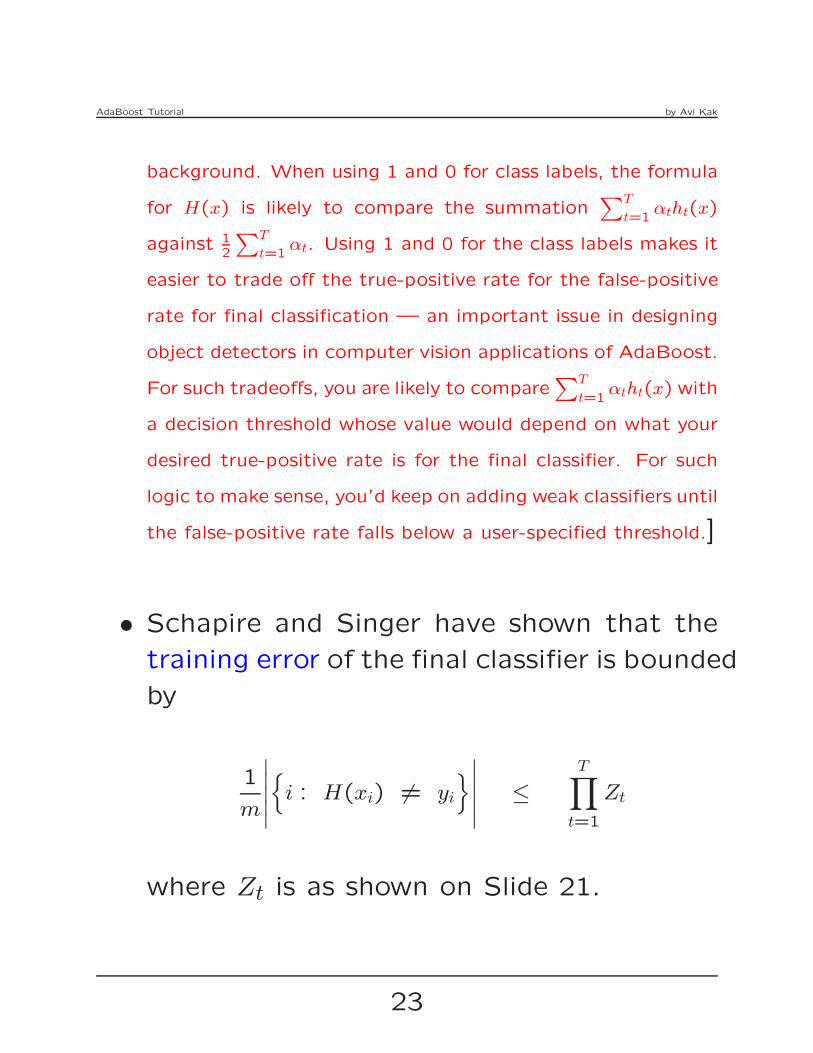
background. When using 1 and 0 for class labels, the formula
for H(x) is likely to compare the summation∑T
t=1αtht(x)
against 12
∑T
t=1αt. Using 1 and 0 for the class labels makes it
easier to trade off the true-positive rate for the false-positive
rate for final classification — an important issue in designing
object detectors in computer vision applications of AdaBoost.
For such tradeoffs, you are likely to compare∑T
t=1αtht(x) with
a decision threshold whose value would depend on what your
desired true-positive rate is for the final classifier. For such
logic to make sense, you’d keep on adding weak classifiers until
the false-positive rate falls below a user-specified threshold.]
• Schapire and Singer have shown that the
training error of the final classifier is bounded
by
1
m
∣
∣
∣
∣
∣
{
i : H(xi) 6= yi
}
∣
∣
∣
∣
∣
≤
T∏
t=1
Zt
where Zt is as shown on Slide 21.
23

AdaBoost Tutorial by Avi Kak
• The bound shown above implies that for
any value of T , which is the number of
weak classifiers used, you want to use those
that yield the smallest values for {Zt|t =
1 . . . T}. Generalizing this argument to treat-
ing T on a running basis, from amongst all
the weak classifiers at your disposal, you
want to pick that classifier for each iter-
ation t that has the least misclassification
rate.
• If you examine the formula for Zt on Slide
21, the smaller the misclassification rate
for a given weak classifier, the smaller the
associated Zt. Now you can see why in
the comment block on Slide 15, at each
iteration t, we wanted a feature for ht that
minimized ǫt as measured over all of the
training data.
24

AdaBoost Tutorial by Avi Kak
6. An Example for Illustrating AdaBoost
• We will use the two-class example shown
below to illustrate AdaBoost.
• The red points were generated by the Perl
script shown on the next slide. We will
refer to the red points as the “red circles”
or as just “circles”.
25

AdaBoost Tutorial by Avi Kak
• Here is the script for the red circle points:sub gen_points_in_circle {
my @points_in_circle;foreach my $i (0..$N1-1) {
my ($x,$y) = (1,1);while ( ($x**2 + $y**2) >= 1 ) {
$x = Math::Random::random_uniform();$y = Math::Random::random_uniform();
}($x,$y) = (0.4*($x-0.6), 0.4*($y-0.3));push @points_in_circle, ["circle_$i",$x+0.6,$y+0.3];
}return \@points_in_circle;
}
where $N1 specifies the number of points
you want in a circle of radius ≈ 0.4 centered
at (0.6,0.3).
• The green “square” points in the figure aregenerated by the following Perl script:sub gen_points_in_rest_of_square {
my @points_in_square;foreach my $i (0..$N2-1) {
my ($x,$y) = (0.6,0.3);while ( (($x-0.6)**2 + ($y-0.3)**2) < 0.2**2 ) {
$x = Math::Random::random_uniform();$y = Math::Random::random_uniform();
}push @points_in_square, ["square_$i",$x,$y];
}return \@points_in_square;
}
26

AdaBoost Tutorial by Avi Kak
• In the second script on the previous slide,
the variable $N2 controls the number of green
square points you want in the rest of the
[0,1] × [0,1] box shown in the figure on
Slide 25.
• Note that we make no attempt to gen-
erate the training data points according
to any particular statistical distribution in
the respective domains. For example, the
red circle points are NOT uniformly dis-
tributed (despite the impression that may
be created by calls to Math::Random::random uniform)
in the area where they predominate. Along
the same lines, the green square points are
NOT uniformly distributed in the rest of
the [0,1]× [0,1] box. How the red and the
green points are statistically distributed is
NOT important to our illustration of Ad-
aBoost.
27

AdaBoost Tutorial by Avi Kak
• We can use any of a number of approaches
for solving the classification problem de-
picted in the figure on Slide 25. For exam-
ple, it would be trivial to construct an SVM
classifier for this case. Simpler still, an NN
classifier would in all likelihood work just
as well (although it would be a bit slower
for obvious reasons).
• The next section demonstrates how we can
use AdaBoost to solve this problem.
28

AdaBoost Tutorial by Avi Kak
7. Weak Classifiers in Our Example
Study
• A weak classifier for our example will be a
linear decision line as shown in the figure
below. Such a classifier will declare all of
the data points on one side of the line as
being “red circles” and the data points on
the other side as being “green squares”.
L
P
θ
d th
Decision Line
Class "circles"
Class "squares"
(0,0) (1,0)
(1,1)(0,1)
29

AdaBoost Tutorial by Avi Kak
• This sort of a classifier is characterized by
the triple (θ, dth, p), where θ is the orien-
tation of the decision line L, and dth the
threshold on the projections of the data
points on the perpendicular P to L (with
the stipulation that the perpendicular pass
through the origin). We say that the po-
larity p of the classifier is 1 if it classifies
all of the data points whose projections are
less than or equal to dth as being “circle”
and all the data points whose projections
are greater than dth as being “square”. For
the opposite case, we consider the classi-
fier’s polarity to be -1.
• Although, for a given orientation θ, the de-
cision line L constitutes a weak classifier
for almost every value of dth (as long we
choose a polarity that yields a classification
error rate of less than 0.5), that will NOT
be our approach to the construction of a
set of weak classifiers.
30
AdaBoost Tutorial by Avi Kak
• For the discussion that follows, for each
orientation θ, we will choose that decision
line L as our weak classifier which yields
the smallest classification error.
• In our demonstration of AdaBoost, each it-
eration of the algorithm randomly chooses
a value for the orientation θ of the deci-
sion line L. Subsequently we step along
the perpendicular P to L to find the best
value for the threshold dth and the best po-
larity for the classifier. Best means yielding
the least classification error.
• The script that is shown on Slides 30 and
31 demonstrates how we search for the
best weak classifier for a given orientation
θ for the decision line. In lines 7 and 8, the
script first constructs a unit vector along
the perpendicular P to the decision line L.
31

AdaBoost Tutorial by Avi Kak
• At this point, it’s good to recall that, in
general, only a portion of the training data
is used for the training of each weak clas-
sifier. See Slide 19.
• The training data for the current weak clas-
sifier is sorted in lines 10 through 21 in the
ascending order of the data projections on
P .
• Subsequently, in lines 25 through 36, the
script steps through these projection points
on P , from the smallest value to the largest,
and at, each projection point on the per-
pendicular P , it calculates two types of
classification errors that are described next.
Let the projection point under considera-
tion be denoted s.
32

AdaBoost Tutorial by Avi Kak
• The first type of classification error cor-
responds to the case when the predicted
labels for all the data points whose projec-
tions are less than or equal to s are consid-
ered to be ”circle” and all the data points
whose projections are greater than s as be-
ing ”square”.
• The second type of the classification error
corresponds to the opposite case. That
is, when all the data points whose projec-
tions are less than or equal to s are labeled
“square”, and all the data points whose
projections are greater than s are labeled
“circle”.
• In the script, these two types of errors are
stored in the hashes %type_1_errors and %type_2_errors.
33

AdaBoost Tutorial by Avi Kak
• The polarity of the weak classifier chosen
for a given θ is determined by which of the
two minimum values for the two types of
errors is the least. And dth is the corre-
sponding threshold.
• Lines 37 through 42 sort the two types of
errors stored in the hashes %type_1_errors and
%type_2_errors in order to determine which type
of error is the least. The type that yields
the smallest value determines the polarity
of the weak classifier, as set in line 43.
• Subsequently, in lines 44 through 47, we
find the decision threshold dth that corre-
sponds to the best weak classifier for the
decision line orientation used.
34

AdaBoost Tutorial by Avi Kak
sub find_best_weak_linear_classifier_at_given_orientation {1 my $orientation = shift;2 my $training_sample_array_ref = shift;3 my @training_samples = @{$training_sample_array_ref};4 my $polarity;5 my $PI = 3.14159265358979;6 my $orient_in_rad = $orientation * $PI / 180.0;7 my @projection_vec = (-1.0 * sin($orient_in_rad),8 cos($orient_in_rad));9 my %projections;10 foreach my $label (@training_samples) {11 my $projection = $all_sample_labels_with_data{$label}->[0] *12 $projection_vec[0] +13 $all_sample_labels_with_data{$label}->[1] *14 $projection_vec[1];15 $projections{$label} = $projection;16 }17 # Create a sorted list of class labels along the perpendicular18 # line P with the sorting criterion being the location of the19 # projection point20 my @sorted_projections = sort {$projections{$a} <=>21 $projections{$b}} keys %projections;22 my (%type_1_errors, %type_2_errors);23 my $how_many_circle_labels = 0;24 my $how_many_square_labels = 0;25 foreach my $i (0..@sorted_projections-1) {26 $how_many_circle_labels++ if $sorted_projections[$i] =~27 /circle/;28 $how_many_square_labels++ if $sorted_projections[$i] =~29 /square/;30 my $error1 = ($N1 - $how_many_circle_labels +31 $how_many_square_labels) / (1.0 * ($N1 + $N2));32 $type_1_errors{$sorted_projections[$i]} = $error1;33 my $error2 = ($how_many_circle_labels + $N2 -34 $how_many_square_labels) / (1.0 * ($N1 + $N2));35 $type_2_errors{$sorted_projections[$i]} = $error2;36 }
35

AdaBoost Tutorial by Avi Kak
37 my @sorted_type_1_errors = sort {$type_1_errors{$a} <=>
38 $type_1_errors{$b}} keys %type_1_errors;
39 my @sorted_type_2_errors = sort {$type_2_errors{$a} <=>
40 $type_2_errors{$b}} keys %type_2_errors;
41 my $least_type_1_error = $type_1_errors{$sorted_type_1_errors[0]};
42 my $least_type_2_error = $type_2_errors{$sorted_type_2_errors[0]};43 $polarity = $least_type_1_error <= $least_type_2_error ? 1 : -1;
44 my $error_for_polarity =$least_type_1_error <= $least_type_2_error ?
45 $least_type_1_error : $least_type_2_error;
46 my $thresholding_label =$least_type_1_error <= $least_type_2_error ?
47 $sorted_type_1_errors[0] : $sorted_type_2_errors[0];
48 return [$orientation, $projections{$thresholding_label}, $polarity,49 $error_for_polarity];
}
• The next section presents the calling sub-
routine for the function shown above. That
subroutine constitutes an implementation
of the Steps 1 through 6 of Section 5.
36

AdaBoost Tutorial by Avi Kak
8. An Implementation of the AdaBoost
Algorithm
• We next present a Perl implementation of
the Steps 1 through 6 of the AdaBoost
algorithm as shown in Section 5.
• The script shown on Slides 35 and 36 starts
out in lines 4 through 14 by selecting a
subset of the training data on the basis
of the current probability distribution over
the data. The criterion used for choosing
the training samples is very simple: We
sort all the training samples in a descending
order according to their probability values.
We pick the top-ranked training samples by
stepping through the sorted list until the
accumulated probability mass is 0.5.
37

AdaBoost Tutorial by Avi Kak
• A more sophisticated approach to the se-
lection of training samples according to a
given probability distribution over the data
would consist of using an MCMC (Markov-
Chain Monte-Carlo) sampler. [See Section 3.4
of my tutorial “Monte Carlo Integration in Bayesian Estima-
tion” for an introduction to MCMC sampling.]
• For a Perl based implementation of MCMC
sampling with the Metropolis-Hastings al-
gorithm, see my “Random Point Genera-
tor” module available at:
http://search.cpan.org/~avikak/Algorithm-RandomPointGenerator-1.
01/lib/Algorithm/RandomPointGenerator.pm
If copy-and-paste of this long URL is incon-
venient, you can also access this module by
Googling with a query string like “avi kak
cpan random point generator”.
38

AdaBoost Tutorial by Avi Kak
• If you do not want to go the MCMC sam-pling route, but you would like to be a bitmore sophisticated than the approach out-lined in red in the second bullet on Slide 37,you could try the following method: You first
create a fine grid in the [0,1] × [0,1] box, with its resolution
set to the smallest of the intervals between the adjacent point
coordinates along x and y. You would then allocate to each
training sample a number of cells proportional to its prob-
ability. Subsequently, you would fire up a random-number
generator for the two values needed for x and y. The two
such random values obtained would determine the choice of
the training sample for each such two calls to the random
number generator.
• Going back to explaining the code on Slides37 and 38, in lines 15 through 19, the scriptfires up the random number generator foran orientation for the weak classifier forthe current iteration of the AdaBoost al-gorithm. It makes sure that the orientationselected is different from those used previ-ously.
39

AdaBoost Tutorial by Avi Kak
• The decision line orientation selected is stored
in the array @ORIENTATIONS_USED.
• The decision-line orientation chosen and
the training samples selected are shipped
off in lines 21 through 24 to the subroutine
find_best_weak_linear_classifier_ at_given_orientation() that
was presented in the previous section.
• Next, in lines 33 through 40, the script ap-
plies the weak classifier returned by the call
shown in the previous bullet to all of the
training data in order to assess its classifi-
cation error rate. This corresponds to Step
3 on Slide 20. This part of the code makes
a call to the subroutine weak_classify() that is
presented in the next section.
40

AdaBoost Tutorial by Avi Kak
• Calculation of the classification error rate
is followed in line 42 by a calculation of
the trust factor α for the weak classifier
in the current iteration of the AdaBoost
algorithm.
• Subsequently, in lines 43 through 65, we
update the probability distribution over all
the training samples according to Step 5
on Slide 18.
• Starting on Slide 44, the next section presents
the support routines needed by the Perl
code discussed so far.
41

AdaBoost Tutorial by Avi Kak
sub adaboost {1 my @weak_classifiers;2 my $decision_line_orientation = 0;3 foreach my $t (0..$NUMBER_OF_WEAK_CLASSIFIERS-1) {4 my @samples_to_be_used_for_training = ();5 # Select training samples for the current weak classifier:6 my $probability_mass_selected_samples = 0;7 foreach my $label (sort {$PROBABILITY_OVER_SAMPLES{$b} <=>
8 $PROBABILITY_OVER_SAMPLES{$a} }9 keys %PROBABILITY_OVER_SAMPLES) {10 $probability_mass_selected_samples +=11 $PROBABILITY_OVER_SAMPLES{$label};12 last if $probability_mass_selected_samples > 0.5;13 push @samples_to_be_used_for_training, $label;14 }15 while (contained_in($decision_line_orientation,16 @ORIENTATIONS_USED)) {
17 $decision_line_orientation = int(180 *18 Math::Random::random_uniform());19 }20 push @ORIENTATIONS_USED, $decision_line_orientation;21 my $learned_weak_classifier =22 find_best_weak_linear_classifier_at_given_orientation(23 $decision_line_orientation,24 \@samples_to_be_used_for_training);25 $LEARNED_WEAK_CLASSIFIERS{$t} = $learned_weak_classifier;
26 my ($orientation, $threshold,27 $polarity, $error_over_training_samples) =28 @{$learned_weak_classifier};29 # Now find the overall classification error (meaning error30 # for all data points) for this weak classifier. That will31 # allows us to calculate how much confidence we can place in32 # this weak classifier:33 my $error = 0;34 foreach my $label (@all_sample_labels) {35 my $data_point = $all_sample_labels_with_data{$label};
42

AdaBoost Tutorial by Avi Kak
36 my $predicted_label = weak_classify($data_point,37 $orientation, $threshold, $polarity);
38 $error += $PROBABILITY_OVER_SAMPLES{$label}
39 unless $label =~ /$predicted_label/;
40 }
41 push @WEAK_CLASSIFIER_ERROR_RATES, $error;
42 $ALL_ALPHAS[$t] = 0.5 * log((1 - $error) / $error);43 my %new_probability_over_samples;
44 for my $label (keys %PROBABILITY_OVER_SAMPLES) {
45 my $data_point_for_label =
46 $all_sample_labels_with_data{$label};
47 my $predicted_label = weak_classify($data_point_for_label,
48 $orientation, $threshold, $polarity);49 my $exponent_for_prob_mod =$label =~ /$predicted_label/ ?
50 -1.0 : 1.0;
51 $new_probability_over_samples{$label} =
52 $PROBABILITY_OVER_SAMPLES{$label} *
53 exp($exponent_for_prob_mod * $ALL_ALPHAS[$t]);
54 }55 my @all_new_probabilities =
56 values %new_probability_over_samples;
57 my $normalization = 0;
58 foreach my $prob (@all_new_probabilities) {
59 $normalization += $prob;
60 }
61 for my $label (keys %new_probability_over_samples) {62 $PROBABILITY_OVER_SAMPLES{$label} =
63 $new_probability_over_samples{$label}
64 / $normalization;
65 }
66 }
}
43

AdaBoost Tutorial by Avi Kak
9. Some Support Routines
• Line 36 of the script shown in the previ-ous section makes a call to the subroutineweak_classify() shown below:
sub weak_classify {1 my $data_point = shift;2 my $decision_line_orientation = shift;3 my $decision_threshold = shift;4 my $polarity = shift;5 my $PI = 3.14159265358979;6 my $orient_in_rad = $decision_line_orientation * $PI / 180.0;7 # The following defines the pass-through-origin perp to8 # the decision line:9 my @projection_vec = (-1.0 * sin($orient_in_rad),10 cos($orient_in_rad));11 my $projection = $data_point->[0] * $projection_vec[0] +12 $data_point->[1] * $projection_vec[1];13 return $projection <= $decision_threshold ?14 "circle" : "square" if $polarity == 1;15 return $projection <= $decision_threshold ?16 "square" : "circle" if $polarity == -1;}
• The subroutine shown above takes four ar-
guments that we describe in the next bul-
let.
44

AdaBoost Tutorial by Avi Kak
• The first argument, stored in the local vari-
able $data_point in line 1, is for the (x, y) coor-
dinates of the point that needs to be clas-
sified. The second, stored in the local vari-
able $decision_line_orientation, is for the orienta-
tion of the decision line for the weak classi-
fier. The third, stored in $decision_threshold, is
for supplying to the subroutine the value
for dth. And the last, stored in $polarity,
is for the polarity of the weak classifier.
The logic of how the weak classifier works
should be obvious from the code in lines
9 through 16. We first construct a unit
vector along the perpendicular to the de-
cision lines 9 and 10. This is followed by
projecting the training data points on the
unit vector.
• Next let’s consider the implementation of
the final classifier H(x) described on Slide
22. The subroutine final_classify() does this
job and is presented on Slide 43.
45

AdaBoost Tutorial by Avi Kak
• In the loop that starts in line 3 of the code
shown on the next slide, we first extract
in lines 4 and 5 one weak classifier at a
time from all the weak classifiers stored in
the hash %LEARNED_WEAK_CLASSIFIERS. In lines 6 and
7, we call on the weak_classify() presented on
Slide 44 to classify our new data point.
• Subsequently, in lines 8 through 17, we for-
mat the numbers associated with the weak
classifiers in order to produce an output
that is easy to read and that allows for
the different weak classifier performances
to be compared easily. This formatting al-
lows for the sort of a printout shown on
Slide 54.
• We aggregate the individual weak classifi-
cation results in lines 25 through 33 ac-
cording to the formula shown on Slide 22.
46

AdaBoost Tutorial by Avi Kak
sub final_classify {1 my $data_point = shift;
2 my @classification_results;3 foreach my $t (0..$NUMBER_OF_WEAK_CLASSIFIERS-1) {
4 my ($orientation, $threshold, $polarity, $error) =
5 @{$LEARNED_WEAK_CLASSIFIERS{$t}};6 my $result = weak_classify($data_point, $orientation,
7 $threshold, $polarity);8 my $error_rate = $WEAK_CLASSIFIER_ERROR_RATES[$t];
9 $error_rate =~ s/^(0\.\d\d)\d+$/$1/;10 $threshold =~ s/^(-?\d?\.\d\d)\d+$/$1/;
11 $threshold = $threshold < 0 ? "$threshold" : " $threshold";12 if (length($orientation) == 1) {
13 $orientation = " $orientation";
14 } elsif (length($orientation) == 2) {15 $orientation = " $orientation";
16 }17 $polarity = $polarity > 0 ? " $polarity" : $polarity;
18 print "Weak classifier $t (orientation: $orientation " .19 "threshold: $threshold polarity: $polarity " .
20 "error_rate: $error_rate): $result\n";
21 push @classification_results, $result;22 }
23 #For weighted pooling of the results returned by the different24 #classifiers, treat "circle" as +1 and "square" as -1
25 @classification_results = map {s/circle/1/;$_}26 @classification_results;
27 @classification_results = map {s/square/-1/;$_}28 @classification_results;
29 print "classifications: @classification_results\n";
30 my $aggregate = 0;31 foreach my $i (0..@classification_results-1) {
32 $aggregate += $classification_results[$i] * $ALL_ALPHAS[$i];33 }
34 return $aggregate >= 0 ? "circle" : "square";}
47

AdaBoost Tutorial by Avi Kak
10. Using the Demonstration Code in an
Interactive Session
• All of the code shown so far is in the script
file AdaBoost.pl that you will find in the
gzipped tar archive available from the URL:
https://engineering.purdue.edu/kak/distAdaBoost/AdaBoostScripts.tar.gz
• After you have unzipped and untarred the
archive, executing the script AdaBoost.pl
will place you in an interactive session in
which you will be asked to enter the (x, y)
coordinates of a point to classify in the
[0,1]× [0,1] box. The script will then pro-
vide you with the “circle” versus “square”
classification for the point you entered. Be-
fore going into the details of this interac-
tive session, let’s first see what all is done
by the AdaBoost.pl script.
48

AdaBoost Tutorial by Avi Kak
• The script AdaBoost.pl needs values for the
following three user-defined global variables.
The values currently set are shown below.
But, obviously, you can change them as
you wish.
# USER SPECIFIED GLOBAL VARIABLES:my $N1 = 100; # These are the "circle" points in Slide 25my $N2 = 100; # Points outside the circle but inside the
# rest of the [0,1]x[0,1] box. We refer to# to these points as "square" in Slide 25
my $NUMBER_OF_WEAK_CLASSIFIERS = 10;
• With regard to what it accomplishes, the
AdaBoost.pl script first calls the two func-
tions shown on Slide 26 for generating the
number of points specified through the global
variables $N1 and $N2.
• Subsequently, it initializes the probability
distribution over the training samples, as
mentioned by the second bullet on Slide
13.
49

AdaBoost Tutorial by Avi Kak
• Finally, AdaBoost.pl calls the following sub-routines:
display_points_in_each_class( $outputstream );visualize_data();adaboost( $outputstream );interactive_demo();
where the first two calls are for the visu-alization of the training data. The call to
adaboost() accomplishes what was explainedin Section 8 of this tutorial. The last call
above, interactive demo() places the script inan interactive mode in which the user is
prompted for the points (x, y) to classifyand the script returns the final classifica-
tions for the points, while also displayingthe results produced by each weak classi-
fier.
• Note the argument $outputstream in the callsto display_points_in_each_class() and adaboost(). The
role played by this argument is explained onthe next slide.
50

AdaBoost Tutorial by Avi Kak
• The value of the variable $outputstream is set
at the very beginning when you fire up the
script AdaBoost.pl depending on how you re-
spond to the two prompts generated by
the script. These prompts ask you whether
you want the information related to the
construction of the weak classifiers to be
dumped in a file or to be displayed in your
terminal window.
• When you are first becoming familiar with
this Perl code, I recommend that you an-
swer ’no’ to the two prompts. With that
answer, no information related to the weak
classifiers will be put out.
• Shown on the next slide is the code for
interactive_demo():
51

AdaBoost Tutorial by Avi Kak
sub interactive_demo {
1 # The following regex is from perl docs:2 my $_num_regex = ’^[+-]?\ *(\d+(\.\d*)?|\.\d+)([eE][+-]?\d+)?$’;
3 print "\n\nThis AdaBoost demonstration is based on the " .
4 "following randomly selected decision line orientations " .
5 "for the weak classifiers: @ORIENTATIONS_USED\n\n";
6 for (;;) {
7 print "\n\nEnter the coordinates of the point you wish to " .8 "classify: ";
9 my $answer = <STDIN>;
10 die "End of interactive demonstration" unless $answer;
11 next if $answer =~ /^\s*$/;
12 my @nums = split / /, $answer;
13 unless (($nums[0] =~ /$_num_regex/) &&14 ($nums[1] =~ /$_num_regex/)) {
15 print "You entered an illegal character. Try again " .
16 "or enter Contrl-D to exit\n";
17 next;
18 }
19 my $predicted_class = final_classify(\@nums);20 print "The predicted class for the data point: " .
21 "$predicted_class\n";
22 }
}
• The user-interactive script shown above starts
out in lines 3 through 5 by printing out the
decision line orientations selected for the
weak classifiers.
52

AdaBoost Tutorial by Avi Kak
• The rest of the script on the previous slide
is an infinite loop in which the user is asked
for the (x, y) coordinates of a point in the
[0,1]×[0,1] box that needs to be classified.
In lines 13 through 17, the script makes
sure that the information entered by the
user is indeed a pair of floating point num-
bers.
• Finally, in line 19, it calls the final_classify()
function of the previous section to classify
the point.
• A command-line invocation such as
AdaBoost.pl
automatically places the script in the inter-
active mode.
53
AdaBoost Tutorial by Avi Kak
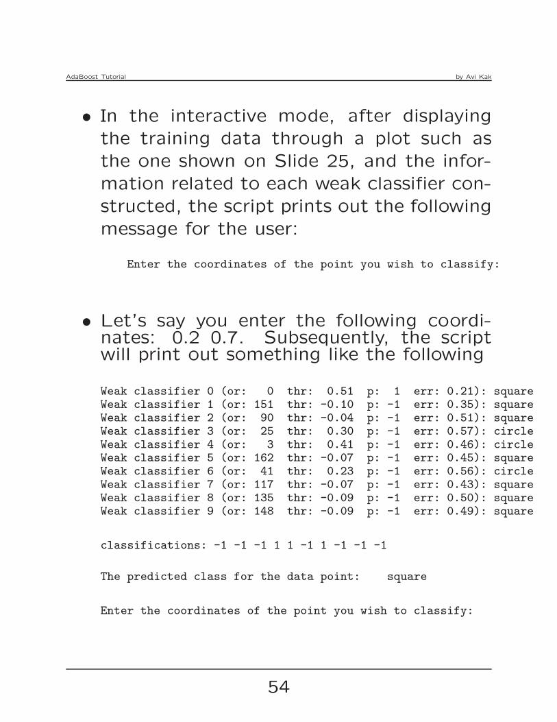
• In the interactive mode, after displaying
the training data through a plot such as
the one shown on Slide 25, and the infor-
mation related to each weak classifier con-
structed, the script prints out the following
message for the user:
Enter the coordinates of the point you wish to classify:
• Let’s say you enter the following coordi-nates: 0.2 0.7. Subsequently, the scriptwill print out something like the following
Weak classifier 0 (or: 0 thr: 0.51 p: 1 err: 0.21): squareWeak classifier 1 (or: 151 thr: -0.10 p: -1 err: 0.35): squareWeak classifier 2 (or: 90 thr: -0.04 p: -1 err: 0.51): squareWeak classifier 3 (or: 25 thr: 0.30 p: -1 err: 0.57): circleWeak classifier 4 (or: 3 thr: 0.41 p: -1 err: 0.46): circleWeak classifier 5 (or: 162 thr: -0.07 p: -1 err: 0.45): squareWeak classifier 6 (or: 41 thr: 0.23 p: -1 err: 0.56): circleWeak classifier 7 (or: 117 thr: -0.07 p: -1 err: 0.43): squareWeak classifier 8 (or: 135 thr: -0.09 p: -1 err: 0.50): squareWeak classifier 9 (or: 148 thr: -0.09 p: -1 err: 0.49): square
classifications: -1 -1 -1 1 1 -1 1 -1 -1 -1
The predicted class for the data point: square
Enter the coordinates of the point you wish to classify:
54

AdaBoost Tutorial by Avi Kak
• In the display you see on the previous slide,
I have abbreviated some of the labels the
script prints out so as not to overflow the
page boundaries. The ’or’ label is actually
printed out as ’orientation’, the ’thr’ label
as ’threshold’, ’p’ as ’polarity’, and, finally,
the ’err’ label as ’error rate’.
• You can exit the interactive session by en-
tering 〈Ctrl−d〉 in response to the prompt.
55

AdaBoost Tutorial by Avi Kak
11. Introduction to Codeword-Based
Learning for Solving Multiclass Problems
• The rest of this tutorial is concerned with
using AdaBoost when you have more than
two classes to deal with.
• A not-so-uncommon way to use a binary
classifier (such as, say, SVM or AdaBoost)
for solving a multiclass classification prob-
lem is to devise a set of binary classifiers,
with each binary classifier comparing one
class against all the others. So if your data
is modeled by Nc classes, you would need
Nc one-versus-the-rest binary classifiers for
solving the problem.
• In this tutorial, we will use a different strat-
egy for solving a multiclass classification
problem with AdaBoost. This strategy is
based on codeword based learning.
56

AdaBoost Tutorial by Avi Kak
• So what’s codeword based learning of mul-
ticlass discriminations?
• The next several bullets explain this new
idea that was first introduced by Dietterich
and Bakiri in their seminal paper “Solv-
ing Multiclass Learning Problems via Error-
Correcting Output Codes,” Journal of Ar-
tificial Intelligence Research, 1995. The
example that I present to explain codeword
based learning is drawn from the introduc-
tion to the paper by Dietterich and Bakiri
• Consider the problem of digit recognition in
handwritten material. We want to assign
a digit to one of ten classes. A structural
approach to solving this problem consists
of identifying the presence or absence of six
features in each digit and basing the final
classification on which features are found
to be present and which ones to be absent.
57

AdaBoost Tutorial by Avi Kak
• The six structural features are:
vl: contains vertical linehl: contains horizontal linedl: contains diagonal linecc: contains close curveol: contains curve open to the leftor: contains curve open to the right
• The presence or the absence of these fea-
tures for each of the 10 digit classes may
now be indicated by the following codeword
matrix:
Class vl hl dl cc ol or---------------------------------------------
0 0 0 0 1 0 01 1 0 0 0 0 02 0 1 1 0 1 03 0 0 0 0 1 04 1 1 0 0 0 05 1 1 0 0 1 06 0 0 1 1 0 17 0 0 1 0 0 08 0 0 0 1 0 09 0 0 1 1 0 0
Note that each row in the table shown
above is distinct so that each digit has a
unique codeword.
58

AdaBoost Tutorial by Avi Kak
• Let’s now assume that we only have bi-
nary classifiers at our disposal. How can
we use such classifiers to solve the multi-
class recognition problem presented on the
previous slide?
• If all we have are binary classifiers, each
column of the matrix presented on the pre-
vious slide can be learned by a binary clas-
sifier from all of the training data in the
following manner: Let’s say we have 1000 training
samples of handwritten digits available to us, distributed uni-
formly with respect to all the ten digits. For the learning of
the first column, we divide the set of training samples into
two halves, one containing the digits labeled 1, 4, and 5, and
the other containing the digits labeled 0, 2, 3, 6, 7, 8, and 9.
We now use an SVM or AdaBoost to create a binary classi-
fier for making a distinction between these TWO categories,
the first corresponding to the digits 1, 4, and 5 and the sec-
ond category corresponding to the rest. We can refer to this
binary classifier as f vl.
59

AdaBoost Tutorial by Avi Kak
• In this manner, we construct six binary clas-
sifiers, one for each column of the code-
word matrix on Slide 58. We may labels
the six binary classifiers as
f_vl f_hl f_dl f_cc f_ol f_or
• Now when we want to predict the class la-
bel of a new digit, we apply each of these
six binary classifiers to the pixels for the
digit. If the output of each binary clas-
sifier is thresholded to result in 0,1 clas-
sification, the output produced by the six
binary classifiers will be a six-bit codeword
like 110001. We assign to the new digit
the class label of the row of the codeword
matrix which is at the shortest Hamming
distance from the codeword extracted for
the new digit.
60

AdaBoost Tutorial by Avi Kak
• For example, if the six binary classifiers
yielded the codeword 110001 for the new
data, you would give it the class label 4
since, of all the codewords shown in the
matrix above, the Hamming distance from
110001 is the shortest to the codeword
110000 that corresponds to the digit 4.
Recall that the Hamming distance mea-
sures the number of bit positions in which
two codewords differ.
• Does the basic idea of codeword based learn-
ing as presented above suffer from any short-
comings? We examine this issue next.
• If the six features that correspond to the
six columns of the codeword matrix shown
above could be measured precisely, then
the basic approach outlined above should
work perfectly.
61

AdaBoost Tutorial by Avi Kak
• In reality, unfortunately, there will always
be errors associated with the extraction of
those features from a blob of pixels. Yes,
the basic approach does give us a little bit
of wiggle room for dealing with such errors
since we only use 10 out of 32 (= 26) dif-
ferent possible codewords and since Ham-
ming distance is used to map the measured
codeword to the nearest codeword in the
matrix for classification. However, the de-
gree of protection against errors is rather
limited.
• If d is the shortest Hamming distance be-
tween any pair of the codewords in a code-
word matrix, the basic approach protects
us against making at most ⌊d−12 ⌋ errors in
the extraction of the codeword for a new
object to be classified.
62

AdaBoost Tutorial by Avi Kak
• For the codeword matrix shown on Slide
58, the smallest distance is only 1 between
the codewords for the digit 4 and 5. The
distance is also just 1 for the digit 7 and
8 and for 8 and 9. What that means is
that the codeword matrix of Slide 58 can-
not tolerate any errors at all in the output
of the six binary classifiers. [Even if we did not
use a set of binary classifiers to learn that codeword matrix
and relied on directly extracting the six structural features
listed at the top of Slide 58, representing the classes in the
manner shown in the matrix of Slide 58 does not allow for
any errors in the extraction of the six features.]
• Let’s now see how the basic idea of a code-
word matrix can be generalized to give us
greater protection against measurement er-
rors.
63

AdaBoost Tutorial by Avi Kak
• The idea that is used for the generalization
we need is based on what’s known as er-
ror correction coding (ECC) that’s used for
reliable communications over noisy chan-
nels and for increasing the reliability of data
storage in modern computers.
• In the ECC based approach to codeword
matrix design, we are allowed to assign
codewords of arbitrary length (subject to
the constraint that for k classes, you will
have a maximum of 2k columns in the code-
word matrix if you want the columns to be
distinct) to the classes.
• For the 10 classes of digit recognition, here
is an example drawn from the paper by Di-
etterich and Bakiri in which we assign 15-
bit codewords to the classes:
64

AdaBoost Tutorial by Avi Kak
Class f0 f1 f2 f3 f4 f5 f6 f7 f8 f9 f10 f11 f12 f13 f14------------------------------------------------------------------
0 1 1 0 0 0 0 1 0 1 0 0 1 1 0 11 0 0 1 1 1 1 0 1 0 1 1 0 0 1 02 1 0 0 1 0 0 0 1 1 1 1 0 1 0 13 0 0 1 1 0 1 1 1 0 0 0 0 1 0 14 1 1 1 0 1 0 1 1 0 0 1 0 0 0 15 0 1 0 0 1 1 0 1 1 1 0 0 0 0 16 1 0 1 1 1 0 0 0 0 1 0 1 0 0 17 0 0 0 1 1 1 1 0 1 0 1 1 0 0 18 1 1 0 1 0 1 1 0 0 1 0 0 0 1 19 0 1 1 1 0 0 0 0 1 0 1 0 0 1 1
• Note that the columns in the codeword ma-
trix shown above carry no meaning — un-
like the columns in the codeword matrix of
Slide 58 where each column stood for a
visual feature.
• So you can think of the codewords shown
above as having been assigned more or less
arbitrarily to the 10 different classes of in-
terest to us. [As we will soon see, there do exist
certain constraints on how the different codewords are laid
out. Nonetheless, these constraints do not arise from a need
to make the columns of the matrix meaningful in the sense
they are on Slide 58.]
65

AdaBoost Tutorial by Avi Kak
• One thing we can be certain about is that
with so many more codewords possible with
the 15 bits we now use (215 = 32768), we
can make sure that we have a large mini-
mum Hamming distance between any pair
of codewords in the matrix.
• As before, we can use either SVM or Ad-
aBoost classifier for the learning required
for each column of the codeword matrix of
the previous slide. [Let’s denote the binary clas-
sifier for learning the first column by f 0. We can acquire
f 0 by dividing our training samples into two categories, one
with the training samples for the classes {0,2,4,6,8}, and the
other for the classes {1,3,5,7,9}. The purpose of f 0 will be
to discriminate between these two categories. Similarly, to
learn f 1, the binary classifier for the second column of the
codeword matrix, we would need to divide the training data
between the positive examples consisting of the samples for
the classes {0,4,5,8,9} and the negative examples consisting
of the samples for the classes {1,2,3,6,7}. And so on.]
66

AdaBoost Tutorial by Avi Kak
• Dietterich and Bakiri list the following two
criteria for choosing the codewords for the
different classes for solving the multiclass
problem:
1. Row Separation: The minimum Hamming dis-tance between any two rows of the codewordmatrix should be as large as possible.
2. Column Separation: The minimum Hammingdistance between any two columns should belarge. The minimum Hamming distance be-tween any column and the complement of everyother column should also be large.
• The first criterion follows directly from how
the “decoding” step — meaning predicting
a class label for a binary code word as ex-
tracted from a test sample — is supposed
to work (see the last bullet on Slide 60).
67

AdaBoost Tutorial by Avi Kak
• Regarding the second criterion on the pre-
vious slide, it is based on the fact that the
logic of error correction coding (assigning
to a codeword extracted for a new object
the class label for the Hamming-nearest
codeword in the codeword matrix) works
only when the bit-wise errors committed
for the different columns of the codeword
matrix are uncorrelated.
• If two columns are nearly the same, or if
one column is close to being the same as
the complement of another column, the
bit-wise errors for two different positions
in the codeword will be correlated (in the
sense that one error will be predictable from
the other).
68

AdaBoost Tutorial by Avi Kak
• As I said earlier, if you have k classes, the
largest number of columns you can have in
your codeword matrix is 2k. To all these
columns, you must apply the Column Sep-
aration criterion mentioned on the previous
slide.
• The Column Separation criterion makes it
difficult to create codeword matrices for
cases when the number of classes is less
than 5. [For example, when you have only 3 classes,
you have k = 3. In this case, you can have a maximum of 8
(= 23) columns. If you eliminate from these the all-zeros and
the all-ones columns, you are left with only 6 columns. Now
if you eliminate the complements of the columns, you will be
left with only 3 columns for the three classes. That does not
give you much error protection in a codeword based approach
to multiclass learning.]
69

AdaBoost Tutorial by Avi Kak
• The smallest number of classes in which
the codeword based approach to learning
works is k = 5. Dietterich and Bakiri have
provided the following codeword matrix for
this number of classes:
Class f0 f1 f2 f3 f4 f5 f6 f7 f8 f9 f10 f11 f12 f13 f14------------------------------------------------------------------
1 1 1 1 1 1 1 1 1 1 1 1 1 1 1 12 0 0 0 0 0 0 0 0 1 1 1 1 1 1 13 0 0 0 0 1 1 1 1 0 0 0 0 1 1 14 0 0 1 1 0 0 1 1 0 0 1 1 0 0 15 0 1 0 1 0 1 0 1 0 1 0 1 0 1 0
• The above codeword matrix for a 5-class
problem was obtained by exhaustively search-
ing through the different possible 15-bit
codewords for the best set that satisfied
the two criteria on Slide 67.
• In the next section, we will use the code-
word matrix shown above to solve a con-
trived 5-class problem.
70

AdaBoost Tutorial by Avi Kak
12. AdaBoost for Codeword-Based
Learning of Multiclass Discriminations
• In the code that you can download from
the URL:
https://engineering.purdue.edu/kak/distAdaBoost/AdaBoostScripts.tar.gz
in addition to the file AdaBoost.pl that I
have already talked about, you will also find
another file named MulticlassAdaBoost.pl
that is meant for showing how AdaBoost
can be used to learn multiclass discrimina-
tions. [By “multiclass”, I mean more than two classes.]
• Multiclass application of AdaBoost will be
demonstrated on the sort of randomly gen-
erated class distributions shown in the fig-
ure on the next slide.
71

AdaBoost Tutorial by Avi Kak
• When I say that the five distributions in the
above figure are “randomly generated,” what
I mean is that when you work with the code
in an interactive mode, for each interactive
session you will see a different distribution
for the five classes in the figure. Of course,
for each session you can feed in as many
test data points as you wish for classifica-
tion and all of those classifications will be
carried out with the same training data.
72

AdaBoost Tutorial by Avi Kak
• Since you already know how AdaBoost works,
I’ll present this part of the tutorial in a top-
down fashion with regard to the content of
the file MulticlassAdaBoost.pl.
• The file MulticlassAdaBoost.pl starts out
with the declarations:
my $NUMBER_OF_CLASSES = 5;my $N = 20;my $NUMBER_OF_WEAK_CLASSIFIERS = 10;my %CODEWORD_MATRIX;$CODEWORD_MATRIX{0} = [ qw/ 1 1 1 1 1 1 1 1 1 1 1 1 1 1 1 / ];$CODEWORD_MATRIX{1} = [ qw/ 0 0 0 0 0 0 0 0 1 1 1 1 1 1 1 / ];$CODEWORD_MATRIX{2} = [ qw/ 0 0 0 0 1 1 1 1 0 0 0 0 1 1 1 / ];$CODEWORD_MATRIX{3} = [ qw/ 0 0 1 1 0 0 1 1 0 0 1 1 0 0 1 / ];$CODEWORD_MATRIX{4} = [ qw/ 0 1 0 1 0 1 0 1 0 1 0 1 0 1 0 / ];
where the variable $N holds the number of
data samples per class, and the variable
$NUMBER_OF_WEAK_CLASSIFIERS specifies how many weak
classifiers to construct for each column of
the codeword matrix. The codeword ma-
trix shown above is the one recommended
by Dietterich and Bakiri.
73

AdaBoost Tutorial by Avi Kak
• Next, the file MulticlassAdaBoost.pl declares
the following global variables:
my %TRAINING_DATA;my %ALL_SAMPLE_LABELS_WITH_DATA;my %COLUMNS;my $NUMBER_OF_COLUMNS;my %POSITIVE_CLASSES_FOR_ALL_COLUMNS;my %NEGATIVE_CLASSES_FOR_ALL_COLUMNS;my %ORIENTATIONS_USED_FOR_ALL_COLUMNS;my %WEAK_CLASSIFIERS_FOR_ALL_COLUMNS;my %WEAK_CLASSIFIER_ERROR_RATES_FOR_ALL_COLUMNS;my %ALPHAS_FOR_ALL_COLUMNS;
Several of these variables, whose names
should convey the purpose they serve, are
meant for convenience. [While all of the train-
ing data for all the classes is held in the hash %TRAINING DATA
where the keys are the class indexes, we also store the same
data in the hash %ALL SAMPLE LABELS WITH DATA where the keys
are the ”class-x-sample-i” tags associated with the different
data points. The hash %COLUMNS holds the individual columns
of the %CODEWORD MATRIX hash introduced earlier. The keys of
the %COLUMNS hash are the column indexes and the values the
columns of the codeword matrix. The variable $NUMBER OF COLUMNS
is set to the number of columns of the codeword matrix.]
74
AdaBoost Tutorial by Avi Kak
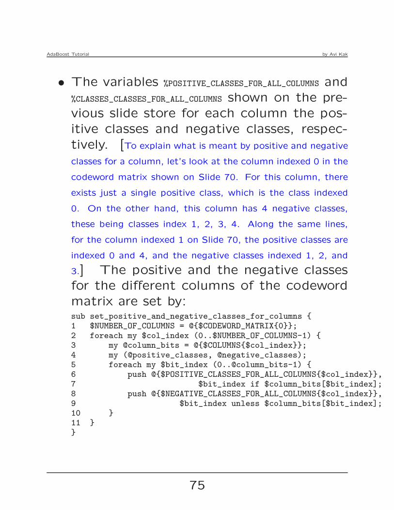
• The variables %POSITIVE_CLASSES_FOR_ALL_COLUMNS and
%CLASSES_CLASSES_FOR_ALL_COLUMNS shown on the pre-
vious slide store for each column the pos-
itive classes and negative classes, respec-
tively. [To explain what is meant by positive and negative
classes for a column, let’s look at the column indexed 0 in the
codeword matrix shown on Slide 70. For this column, there
exists just a single positive class, which is the class indexed
0. On the other hand, this column has 4 negative classes,
these being classes index 1, 2, 3, 4. Along the same lines,
for the column indexed 1 on Slide 70, the positive classes are
indexed 0 and 4, and the negative classes indexed 1, 2, and
3.] The positive and the negative classes
for the different columns of the codeword
matrix are set by:sub set_positive_and_negative_classes_for_columns {1 $NUMBER_OF_COLUMNS = @{$CODEWORD_MATRIX{0}};2 foreach my $col_index (0..$NUMBER_OF_COLUMNS-1) {3 my @column_bits = @{$COLUMNS{$col_index}};4 my (@positive_classes, @negative_classes);5 foreach my $bit_index (0..@column_bits-1) {6 push @{$POSITIVE_CLASSES_FOR_ALL_COLUMNS{$col_index}},7 $bit_index if $column_bits[$bit_index];8 push @{$NEGATIVE_CLASSES_FOR_ALL_COLUMNS{$col_index}},9 $bit_index unless $column_bits[$bit_index];10 }11 }}
75

AdaBoost Tutorial by Avi Kak
• Starting with Slide 79, we show the workhorse
of MulticlassBadaBoost.pl script. It’s this
script’s job to create all of the weak clas-
sifiers for the binary classification for the
positive and the negative examples desig-
nated by the 1’s and the 0’s of a given col-
umn of the codeword matrix. The index of
the column that this script is supposed to
work on is supplied as its argument. In the
script itself, the column index becomes the
value of the local variable $col_index in line 1.
• Lines 2 through 14 of the script on Slide
79 are primarily for initializing the proba-
bility distribution of the training samples in
accordance with the second bullet on Slide
13.
76

AdaBoost Tutorial by Avi Kak
• The search for the weak classifiers begins
in line 20. In lines 21 through 31, we use
the current probability distribution over the
training samples to choose a subset of the
training data for the next weak classifier.
• The logic used in lines 32 through 63 for
the construction of a weak classifier is ex-
actly the same as described in Section 7
of this tutorial. [For a weak classifier, we randomly
choose an orientation for the decision line, an example of
which was shown in the figure on Slide 29. We then move
this decision along its perpendicular until we find a position
where the classification error rate over the training samples
being used is the least. When we find the best position of
the decision line, we take into account both polarities for the
classification rule expressed by the decision line. The best
location of the line on the perpendicular gives us the decision
threshold dth to use for this weak classifier.]
77

AdaBoost Tutorial by Avi Kak
• In lines 65 through 70, we set the value of
αt as required by Step 4 on Slide 20. Note
that the implementation you see for the
calculation of αt differs from its analytical
form on Slide 20. The reason is that the
analytical form shown on Slide 20 becomes
problematic when the error rate ǫt is zero.
As shown in line 69, when the error rate is
less than 0.00001, we clamp αt at a high
value of 5.
• Lines 71 through 103 are devoted to the
calculation of the new probability distribu-
tion over the training samples according to
the classification errors made by the weak
classifier just constructed. This calculation
uses the formula shown in Step 5 on Slide
20.
78

AdaBoost Tutorial by Avi Kak
sub generate_weak_classifiers_for_one_column_of_codeword_matrix {1 my $col_index = shift;2 my @positive_classes =
3 @{$POSITIVE_CLASSES_FOR_ALL_COLUMNS{$col_index}};4 my @negative_classes =
5 @{$NEGATIVE_CLASSES_FOR_ALL_COLUMNS{$col_index}};6 my $N_positives = 0;7 foreach my $class_index (@positive_classes) {
8 $N_positives += @{$TRAINING_DATA{$class_index}};9 }
10 my $N_negatives = 0;11 foreach my $class_index (@negative_classes) {12 $N_negatives += @{$TRAINING_DATA{$class_index}};
13 }14 my $N_total = $N_positives + $N_negatives;15 my %probability_over_samples;
16 foreach my $label (keys %ALL_SAMPLE_LABELS_WITH_DATA) {17 $probability_over_samples{$label} = 1.0 / $N_total;
18 }19 my $decision_line_orientation = 0;20 foreach my $t (0..$NUMBER_OF_WEAK_CLASSIFIERS-1) {
21 my @samples_to_be_used_for_training = ();22 # Select training samples for the current weak classifier:23 my $probability_mass_selected_samples = 0;
24 foreach my $label (sort {$probability_over_samples{$b} <=>25 $probability_over_samples{$a} }
26 keys %probability_over_samples) {27 $probability_mass_selected_samples +=28 $probability_over_samples{$label};
29 last if $probability_mass_selected_samples > 0.8;30 push @samples_to_be_used_for_training, $label;
31 }32 while (contained_in($decision_line_orientation,33 @{$ORIENTATIONS_USED_FOR_ALL_COLUMNS{$col_index}})) {
34 $decision_line_orientation =35 int(180 * Math::Random::random_uniform());
79

AdaBoost Tutorial by Avi Kak
36 }37 push @{$ORIENTATIONS_USED_FOR_ALL_COLUMNS{$col_index}},38 $decision_line_orientation;39 my $learned_weak_classifier =40 find_best_weak_linear_classifier_at_given_orientation(41 $decision_line_orientation, \@positive_classes,42 \@negative_classes );43 push @{$WEAK_CLASSIFIERS_FOR_ALL_COLUMNS{$col_index}},
44 $learned_weak_classifier;45 my ($orientation, $threshold, $polarity,46 $error_over_training_samples) = @{$learned_weak_classifier};47 my $error = 0;48 foreach my $label (keys %ALL_SAMPLE_LABELS_WITH_DATA) {49 my $data_point = $ALL_SAMPLE_LABELS_WITH_DATA{$label};50 my $predicted_label = weak_classify($data_point,51 $orientation, $threshold, $polarity);52 $label =~ /class_(\d+)_sample/;
53 my $class_index_for_label = $1;54 next if (contained_in($class_index_for_label,55 @positive_classes) &&56 ($predicted_label eq ’positive’)) ||57 (contained_in($class_index_for_label,58 @negative_classes) &&59 ($predicted_label eq ’negative’));6061 $error += $probability_over_samples{$label};
62 }63 push @{$WEAK_CLASSIFIER_ERROR_RATES_FOR_ALL_COLUMNS{$col_index}},64 $error;65 if ($error > 0.00001) {66 $ALPHAS_FOR_ALL_COLUMNS{$col_index}->[$t] =67 0.5 * log((1 - $error) / $error);68 } else {69 $ALPHAS_FOR_ALL_COLUMNS{$col_index}->[$t] = 5;70 }71 my %new_probability_over_samples;
80

AdaBoost Tutorial by Avi Kak
72 for my $label (keys %probability_over_samples) {
73 my $data_point_for_label =74 $ALL_SAMPLE_LABELS_WITH_DATA{$label};
75 my $predicted_label = weak_classify($data_point_for_label,
76 $orientation, $threshold, $polarity);
77 my $exponent_for_prob_mod;
78 $label =~ /class_(\d+)_sample/;
79 my $class_index_for_label = $1;80 if ( (contained_in($class_index_for_label,
81 @positive_classes) &&
82 ($predicted_label eq ’positive’)) ||
83 (contained_in($class_index_for_label,
84 @negative_classes) &&
85 ($predicted_label eq ’negative’)) ) {86 $exponent_for_prob_mod = -1.0;
87 } else {
88 $exponent_for_prob_mod = 1.0;
89 }
90 $new_probability_over_samples{$label} =
91 $probability_over_samples{$label} *92 exp($exponent_for_prob_mod *
93 $ALPHAS_FOR_ALL_COLUMNS{$col_index}->[$t]);
94 }
95 my @all_new_probabilities = values %new_probability_over_samples;
96 my $normalization = 0;
97 foreach my $prob (@all_new_probabilities) {
98 $normalization += $prob;99 }
100 for my $label (keys %new_probability_over_samples) {
101 $probability_over_samples{$label} =
102 $new_probability_over_samples{$label} / $normalization;
103 }
104 }}
81

AdaBoost Tutorial by Avi Kak
• Another subroutine that plays a key role in
the codeword based multiclass discrimina-
tions is final classify for one column of codeword matrix()
whose job is to aggregate the classifica-
tions returned by each of the weak classi-
fiers for a given column and return the final
classifications of a new data point. Shown
on the next slide is the implementation of
this subroutine. [This subroutine takes two argu-
ments, the column index and the data point you want to
classify. These become the values of local variables in lines 1
and 2 on the next slide.]
• After fetching the weak classifiers for the
designated column in lines 3 and 4, the
loop in lines 8 through 26 queries each of
the weak classifiers and formats their out-
put for the presentation of the results in
lines 25 through 28.
82

AdaBoost Tutorial by Avi Kak
• For aggregating the results returned by the
individual weak classifiers, we use the for-
mula on Slide 22. This aggregation is im-
plemented in lines 33 through 44.
• Note that the call to weak classify() in line
11 has the same implementation as shown
previously on Slide 43.
sub final_classify_for_one_column_of_codeword_matrix {1 my $col_index = shift;
2 my $data_point = shift;
3 my $number_of_weak_classifiers_for_this_column =
4 scalar( @{$WEAK_CLASSIFIERS_FOR_ALL_COLUMNS{$col_index}} );
5 my @classification_results;
6 my @weak_classifiers_for_this_column =7 @{$WEAK_CLASSIFIERS_FOR_ALL_COLUMNS{$col_index}};
8 foreach my $t (0..$number_of_weak_classifiers_for_this_column-1) {
9 my ($orientation, $threshold, $polarity, $error) =
10 @{$weak_classifiers_for_this_column[$t]};
11 my $result = weak_classify($data_point, $orientation,
12 $threshold, $polarity);13 my $error_rate =
14 $WEAK_CLASSIFIER_ERROR_RATES_FOR_ALL_COLUMNS{$col_index}->[$t];
83

AdaBoost Tutorial by Avi Kak
15 $error_rate =~ s/^(0\.\d\d)\d+$/$1/;
16 $error_rate = " $error_rate" if length($error_rate) == 1;
17 $threshold =~ s/^(-?\d?\.\d\d)\d+$/$1/;
18 $threshold = $threshold < 0 ? "$threshold" : " $threshold";19 if (length($orientation) == 1) {
20 $orientation = " $orientation";
21 } elsif (length($orientation) == 2) {
22 $orientation = " $orientation";
23 }
24 $polarity = $polarity > 0 ? " $polarity" : $polarity;25 print "[Column $col_index] Weak classifier $t " .
26 "(orientation: $orientation threshold: $threshold " .
27 "polarity: $polarity error_rate: $error_rate): " .
28 "$result\n";
29 push @classification_results, $result;
30 }31 #For weighted pooling of the results returned by the different
32 #classifiers, treat "positive" as +1 and "negative" as -1
33 @classification_results =
34 map {s/positive/1/;$_} @classification_results;
35 @classification_results =
36 map {s/negative/-1/;$_} @classification_results;37 print "[Column $col_index] weak classifications:
38 @classification_results\n";
39 my $aggregate = 0;
40 foreach my $i (0..@classification_results-1) {
41 $aggregate += $classification_results[$i] *
42 $ALPHAS_FOR_ALL_COLUMNS{$col_index}->[$i];43 }
44 return $aggregate >= 0 ? "positive" : "negative";
}
84

AdaBoost Tutorial by Avi Kak
13. An Interactive Session That Shows
the Power of a Single Column of
Codeword Matrix as a Binary Classifier
• When you first fire up MulticlassAdaBoost.pl, it
will prompt you for whether you want the
multiclass classifier as learned from the en-
tire codeword matrix, or a single binary
classifier for a single column of the matrix.
If you opt for the latter, the script will en-
ter the column-interactive mode and it will
ask you to enter the column index for the
column you are interested in.
• When you choose the single-column option
in your response to the prompts, the script
invokes the overall interactive() subroutine.
• Shown on Slide 87 is the implementation
of the subroutine column interactive().
85
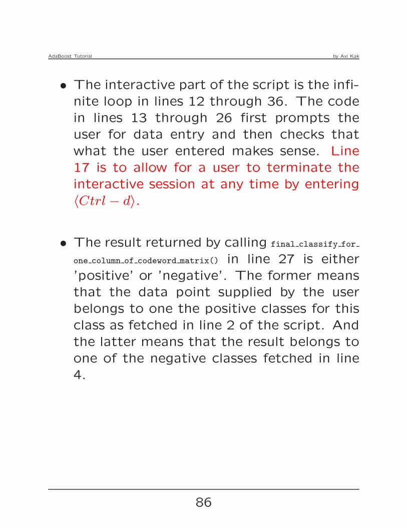
AdaBoost Tutorial by Avi Kak
• The interactive part of the script is the infi-
nite loop in lines 12 through 36. The code
in lines 13 through 26 first prompts the
user for data entry and then checks that
what the user entered makes sense. Line
17 is to allow for a user to terminate the
interactive session at any time by entering
〈Ctrl − d〉.
• The result returned by calling final classify for
one column of codeword matrix() in line 27 is either
’positive’ or ’negative’. The former means
that the data point supplied by the user
belongs to one the positive classes for this
class as fetched in line 2 of the script. And
the latter means that the result belongs to
one of the negative classes fetched in line
4.
86
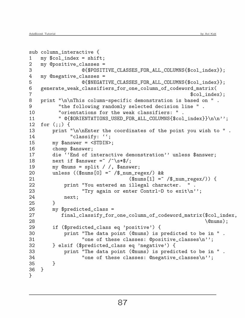
AdaBoost Tutorial by Avi Kak
sub column_interactive {1 my $col_index = shift;2 my @positive_classes =3 @{$POSITIVE_CLASSES_FOR_ALL_COLUMNS{$col_index}};4 my @negative_classes =5 @{$NEGATIVE_CLASSES_FOR_ALL_COLUMNS{$col_index}};6 generate_weak_classifiers_for_one_column_of_codeword_matrix(7 $col_index);8 print "\n\nThis column-specific demonstration is based on " .9 "the following randomly selected decision line " .10 "orientations for the weak classifiers: " .11 " @{$ORIENTATIONS_USED_FOR_ALL_COLUMNS{$col_index}}\n\n’’;12 for (;;) {13 print "\n\nEnter the coordinates of the point you wish to " .14 "classify: ‘‘;15 my $answer = <STDIN>;16 chomp $answer;17 die ‘‘End of interactive demonstration’’ unless $answer;18 next if $answer =~ /^\s*$/;19 my @nums = split / /, $answer;20 unless (($nums[0] =~ /$_num_regex/) &&21 ($nums[1] =~ /$_num_regex/)) {22 print "You entered an illegal character. " .23 "Try again or enter Contrl-D to exit\n’’;24 next;25 }26 my $predicted_class =27 final_classify_for_one_column_of_codeword_matrix($col_index,28 \@nums);29 if ($predicted_class eq ’positive’) {30 print "The data point (@nums) is predicted to be in " .31 "one of these classes: @positive_classes\n’’;32 } elsif ($predicted_class eq ’negative’) {33 print "The data point (@nums) is predicted to be in " .34 "one of these classes: @negative_classes\n’’;35 }36 }}
87

AdaBoost Tutorial by Avi Kak
• When you invoke MulticlassAdaBoost.pl inthe column-interactive mode, you will seea popup window with a plot such as the
one shown on Slide 72 and the followingsort of output in your terminal window:
=> MulticlassAdaBoost.plPrining out the points in class 0:class_0_sample_0 0.0388130199253125 0.306701274378974class_0_sample_1 -0.0483082434657033 0.333167487289401........Prining out the points in class 1:class_1_sample_0 0.439181892150296 0.15767914403357class_1_sample_1 0.341741264689717 0.290947662466462........Prining out the points in class 2:class_2_sample_0 0.62339139639785 0.233743754191426class_2_sample_1 0.663987994007291 0.185020510091793........Prining out the points in class 3:class_3_sample_0 0.0119872353686556 0.505153721523502class_3_sample_1 0.192827443382858 0.416779605628115................Column 0: 1 0 0 0 0Column 1: 1 0 0 0 1Column 2: 1 0 0 1 0Column 3: 1 0 0 1 1........This column-specific demonstration is based on the followingrandomly selected decision line orientations for the weakclassifiers: 0 173 55 37 96 105 174 113 166 30
Enter the coordinates of the point you wish to classify:
You enter the coordinates of the point you
wish to classify in response to the promptyou see at the bottom.
88

AdaBoost Tutorial by Avi Kak
• Let’s say you enter something like “0.2
0.6” in response to the prompt. Next, the
system will come back with the following
sort of classification results for your point:
[Column 5] Weak classifier 0 (.........): positive
[Column 5] Weak classifier 1 (.........): positive
[Column 5] Weak classifier 2 (.........): negative
[Column 5] Weak classifier 3 (.........): negative[Column 5] Weak classifier 4 (.........): negative
[Column 5] Weak classifier 5 (.........): negative
[Column 5] Weak classifier 6 (.........): positive
[Column 5] Weak classifier 7 (.........): negative
[Column 5] Weak classifier 8 (.........): positive
[Column 5] Weak classifier 9 (.........): negative[Column 5] weak classifications: 1 1 -1 -1 -1 -1 1 -1 1 -1
The data point (0.2 0.6) is predicted to be in one of these classes:
Enter the coordinates of the point you wish to classify:
where I have suppressed a lot of informa-
tion regarding each weak classifier that is
printed out inside the parentheses that cur-
rently just have dots.
89

AdaBoost Tutorial by Avi Kak
• Each row of the output shown on the pre-
vious slide starts with the column of the
codeword matrix whose discriminatory power
you are investigating. Recall that any sin-
gle column can only carry out a binary clas-
sification into two groups of classes, those
corresponding to the 1’s in the column and
those corresponding to the 0’s in the col-
umn.
• When a weak classifier reports ’positive’ for
the classification of the point you supplied,
it means that, according to the weak clas-
sifier, the point belongs to the classes cor-
responding to the 1’s in the column. Sim-
ilarly, for the ’negative’ classification.
90

AdaBoost Tutorial by Avi Kak
14. An Interactive Session forDemonstrating Multiclass Classification
with AdaBoost
• If you entered “1” in response to the prompt
when you first fired up MulticlassAdaBoost.pl, the
demo will work in the overall-interactive
mode. In this mode, you will again see
the output that was shown in a highly ab-
breviated form on Slide 88 for the column-
interactive mode of operation of the script.
As mentioned there, the output ends in the
following prompt:
Enter the coordinates of the point you wish to classify:
• You are also shown a plot of the sort you
saw on Slide 72 to help you decide what
coordinates you should supply for classifi-
cation. Let’s say you entered “0.2 0.3” in
response to the question shown above, you
will see the kind of output that is displayed
on the next slide.
91

AdaBoost Tutorial by Avi Kak
[Column 0] Weak classifier 0 (..........): negative[Column 0] Weak classifier 1 (..........): negative........[Column 0] weak classifications: -1 -1 -1 -1 -1 -1 -1 -1 -1 -1[Column 1] Weak classifier 0 (..........): negative[Column 1] Weak classifier 1 (..........): negative........[Column 1] weak classifications: -1 -1 -1 -1 -1 -1 -1 -1 -1 -1[Column 2] Weak classifier 0 (..........): negative[Column 2] Weak classifier 1 (..........): negative........[Column 2] weak classifications: -1 -1 -1 -1 -1 -1 -1 -1 -1 -1[Column 3] Weak classifier 0 (..........): negative[Column 3] Weak classifier 1 (..........): negative........[Column 3] weak classifications: -1 -1 -1 -1 -1 -1 -1 1 -1 -1[Column 4] Weak classifier 0 (..........): negative[Column 4] Weak classifier 1 (..........): positive........[Column 4] weak classifications: -1 1 -1 1 1 -1 -1 -1 -1 -1[Column 5] Weak classifier 0 (..........): positive[Column 5] Weak classifier 1 (..........): positive........[Column 5] weak classifications: 1 1 -1 -1 -1 -1 -1 -1 1 -1[Column 6] Weak classifier 0 (..........): positive[Column 6] Weak classifier 1 (..........): positive........[Column 6] weak classifications: 1 1 -1 -1 -1 -1 -1 -1 -1 -1[Column 7] Weak classifier 0 (..........): positive[Column 7] Weak classifier 1 (..........): positive........[Column 7] weak classifications: 1 1 -1 1 1 1 -1 1 -1 -1[Column 8] Weak classifier 0 (..........): negative[Column 8] Weak classifier 1 (..........): negative................[Column 14] weak classifications: 1 1 1 1 1 1 1 1 1 1Predicted codeword for point (.2 .3) is: 0 0 0 0 0 0 0 0 1 1 1 1 1 1 1Predicted class label for (0.2 0.3): 1 [with Hamming Distance: 0]
Enter the coordinates of the point you wish to classify:
92

AdaBoost Tutorial by Avi Kak
• Note the final classification result near the
bottom of the display on the previous slide.
It says that the predicted class label is ’1’.
It also says that the Hamming distance be-
tween the binary code word obtained from
the 15 columns of the codeword matrix and
the codeword corresponding to class 1 is
zero. In this case, we happen to be right on
target. A cool thing about this user inter-
action is that you can verify the accuracy
of the predicted class label by examining
your point on the plot (like the one shown
on Slide 72) that stays on your screen.
• In the overall-interactive, the data point
you want to classify is handed over to the
function final classify with all columns() whose im-
plementation is shown on the next slide.
93

AdaBoost Tutorial by Avi Kak
sub final_classify_with_all_columns {
1 my $data_point = shift;
2 my @prediction_codeword;
3 foreach my $col_index (0..$NUMBER_OF_COLUMNS-1) {4 generate_weak_classifiers_for_one_column_of_codeword_matrix(
5 $col_index) unless $WEAK_CLASSIFIERS_ALREADY_GENERATED;
6 my $predicted_class =
7 final_classify_for_one_column_of_codeword_matrix(
8 $col_index, $data_point);
9 push @prediction_codeword, 1 if $predicted_class eq ’positive’;10 push @prediction_codeword, 0 if $predicted_class eq ’negative’;
11 }
12 print "\nThe predicted codeword for the data point " .
13 "(@{$data_point}) is: @prediction_codeword\n’’;
14 my $number_of_rows = scalar(keys %CODEWORD_MATRIX);
15 my %hamming_distance;16 foreach my $row_index (0..$number_of_rows-1) {
17 my @codeword = @{$CODEWORD_MATRIX{$row_index}};
18 $hamming_distance{$row_index} = 0;
19 foreach my $bit_index (0..$NUMBER_OF_COLUMNS-1) {
20 $hamming_distance{$row_index}++
21 if $prediction_codeword[$bit_index] !=22 $codeword[$bit_index];
23 }
24 }
25 my @sorted_rows = sort {$hamming_distance{$a} <=>
26 $hamming_distance{$b}} keys %hamming_distance;
27 print "\n\nPredicted class label for (@{$data_point}): " . "28 "$sorted_rows[0] [with Hamming Distance: " .
29 "$hamming_distance{$sorted_rows[0]}]\n’’;
}
94

AdaBoost Tutorial by Avi Kak
• As it must, the subroutine on the previous
slide first calls on generate_weak_classifiers_for_one_
_column_of_codeword_matrix() in line 4 to generate
the weak classifiers for each column of the
codeword matrix.
• Subsequently, in lines 6 and 7, it calls on
final_classify_for_one_column_of_codeword_matrix() to use
weak classifiers for each column to carry
out a binary classification of the new data
point. When the class returned is ’posi-
tive’, the new data point belongs to one of
the classes whose bit is 1 in the column.
Otherwise, its classification would be ’neg-
ative’.
• From the ’positive’ or ’negative’ labels re-
turned for each of the column binary classi-
fiers, we construct a codeword for the new
data point in lines 9 and 10.
95
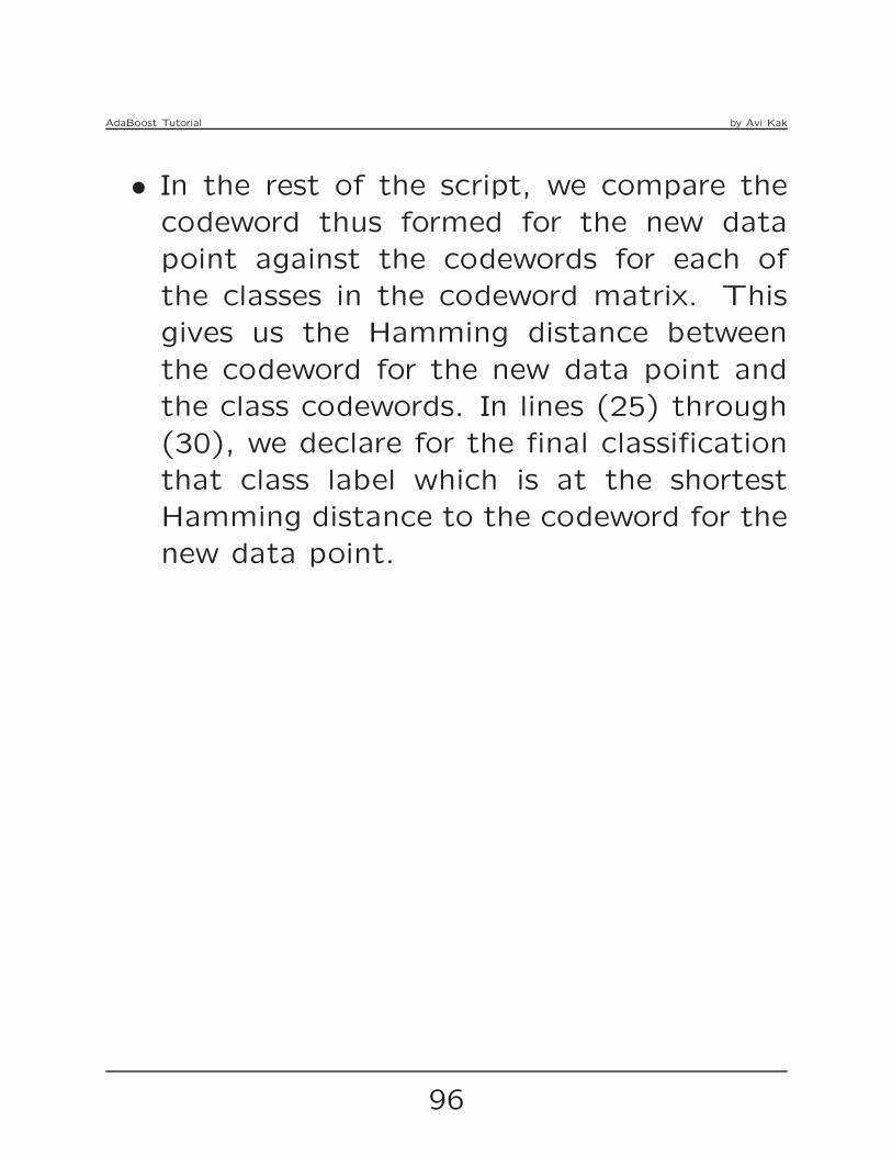
AdaBoost Tutorial by Avi Kak
• In the rest of the script, we compare the
codeword thus formed for the new data
point against the codewords for each of
the classes in the codeword matrix. This
gives us the Hamming distance between
the codeword for the new data point and
the class codewords. In lines (25) through
(30), we declare for the final classification
that class label which is at the shortest
Hamming distance to the codeword for the
new data point.
96

AdaBoost Tutorial by Avi Kak
15. Acknowledgments
This tutorial would not have been possible without all ofthe wonderful things I learned from Guiqin Li, a formergraduate student in RVL.
Several of the more recent changes to the tutorial owetheir origin to some great discussions with Tanmay Prakashwho is wrapping up his Ph.D. dissertation in RVL. He isusing AdaBoost as a feature selection tool for detect-ing infrequently occurring objects in wide-area satelliteimagery.
97


![Multiclass Adaboost Based on an Ensemble of Binary …article.sapub.org/pdf/10.5923.j.ajis.20130302.02.pdf · high classification accuracy of the AdaBoost and the ... Freund and Schapire[10]implemented](https://img.dokumen.tips/doc/110x75/5ae643737f8b9ae1578d64ae/multiclass-adaboost-based-on-an-ensemble-of-binary-classification-accuracy-of.jpg)